Gene set enrichment analysis of RNA-Seq data with …...Gene set enrichment analysis of RNA-Seq data...

Gene set enrichment analysis of RNA-Seq data

with the SeqGSEA package

Xi Wang1,2 and Murray Cairns1,2,3

October 17, 2016

1School of Biomedical Sciences and Pharmacy, The University of Newcastle, Callaghan, New SouthWales, Australia2Hunter Medical Research Institute, New Lambton, New South Wales, Australia3Schizophrenia Research Institute, Sydney, New South Wales, Australia

[email protected]

Contents

1 Introduction 21.1 Background . . . . . . . . . . . . . . . . . . . . . . . . . . . . . . . . . . . . . . . . . 21.2 Getting started . . . . . . . . . . . . . . . . . . . . . . . . . . . . . . . . . . . . . . . 21.3 Package citation . . . . . . . . . . . . . . . . . . . . . . . . . . . . . . . . . . . . . . 2

2 Differential splicing analysis and DS scores 32.1 The ReadCountSet class . . . . . . . . . . . . . . . . . . . . . . . . . . . . . . . . . . 32.2 DS analysis and DS scores . . . . . . . . . . . . . . . . . . . . . . . . . . . . . . . . . 32.3 DS permutation p-values . . . . . . . . . . . . . . . . . . . . . . . . . . . . . . . . . . 5

3 Differential expression analysis and DE scores 63.1 Gene read count data from ReadCountSet class . . . . . . . . . . . . . . . . . . . . . 63.2 DE analysis and DE scores . . . . . . . . . . . . . . . . . . . . . . . . . . . . . . . . 63.3 DE permutation p-values . . . . . . . . . . . . . . . . . . . . . . . . . . . . . . . . . 8

4 Integrative GSEA runs 84.1 DE/DS score integration . . . . . . . . . . . . . . . . . . . . . . . . . . . . . . . . . . 84.2 Initialization of SeqGeneSet objects . . . . . . . . . . . . . . . . . . . . . . . . . . . . 94.3 running GSEA with integrated gene scores . . . . . . . . . . . . . . . . . . . . . . . . 114.4 SeqGSEA result displays . . . . . . . . . . . . . . . . . . . . . . . . . . . . . . . . . . 12

5 Running SeqGSEA with multiple cores 135.1 R-parallel packages . . . . . . . . . . . . . . . . . . . . . . . . . . . . . . . . . . . . . 135.2 Parallelizing analysis on permutation data sets . . . . . . . . . . . . . . . . . . . . . 15

6 Analysis examples 156.1 Starting from your own RNA-Seq data . . . . . . . . . . . . . . . . . . . . . . . . . . 156.2 Exemplified pipeline for integrating DE and DS . . . . . . . . . . . . . . . . . . . . . 156.3 Exemplified pipeline for DE-only analysis . . . . . . . . . . . . . . . . . . . . . . . . 176.4 One-step SeqGSEA analysis . . . . . . . . . . . . . . . . . . . . . . . . . . . . . . . . 18

1

7 Session information 19

1 Introduction

1.1 Background

Transcriptome sequencing (RNA-Seq) has become a key technology in transcriptome studies becauseit can quantify overall expression levels and the degree of alternative splicing for each gene simul-taneously. Many methods and tools, including quite a few R/Bioconductor packages, have beendeveloped to deal with RNA-Seq data for differential expression analysis and thereafter functionalanalysis aiming at novel biological and biomedical discoveries. However, those tools mainly focus oneach gene’s overall expression and may miss the opportunities for discoveries regarding alternativesplicing or the combination of the two.

SeqGSEA is novel R/Bioconductor package to derive biological insight by integrating differentialexpression (DE) and differential splicing (DS) from RNA-Seq data with functional gene set analysis.Due to the digital feature of RNA-Seq count data, the package utilizes negative binomial distributionsfor statistical modeling to first score differential expression and splicing in each gene, respectively.Then, integration strategies are applied to combine the two scores for integrated gene set enrichmentanalysis. See the publications Wang and Cairns (2013) and Wang and Cairns (2014) for moredetails. The SeqGSEA package can also give detection results of differentially expressed genes anddifferentially spliced genes based on sample label permutation.

1.2 Getting started

The SeqGSEA depends on Biobase for definitions of class ReadCountSet and class SeqGeneSet,DESeq for differential expression analysis, biomaRt for gene IDs/names conversion, and doParallelfor parallelizing jobs to reduce running time. Make sure you have these dependent packages installedbefore you install SeqGSEA.

To load the SeqGSEA package, type library(SeqGSEA). To get an overview of this package, type?SeqGSEA.

> library(SeqGSEA)

> ? SeqGSEA

In this Users’ Guide of the SeqGSEA package, an analysis example is given in Section 6, anddetailed guides for DE, DS, and integrative GSEA analysis are given in Sections 3, 2, and 4, respec-tively. A guide to parallelize those analyses is given in Section 5.

1.3 Package citation

To cite this package, please cite the article below:Wang X and Cairns MJ (2014). SeqGSEA: a Bioconductor package for gene set enrichmentanalysis of RNA-Seq data integrating differential expression and splicing. Bioinformatics,30(12):1777-9.

To cite/discuss the method used in this package, please cite the article below:Wang X and Cairns MJ (2013). Gene set enrichment analysis of RNA-Seq data: integratingdifferential expression and splicing. BMC Bioinformatics, 14(Suppl 5):S16.

2

2 Differential splicing analysis and DS scores

2.1 The ReadCountSet class

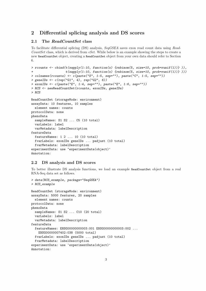
To facilitate differential splicing (DS) analysis, SeqGSEA saves exon read count data using Read-CountSet class, which is derived from eSet. While below is an example showing the steps to create anew ReadCountSet object, creating a ReadCountSet object from your own data should refer to Section6.

> rcounts <- cbind(t(sapply(1:10, function(x) {rnbinom(5, size=10, prob=runif(1))} )),

+ t(sapply(1:10, function(x) {rnbinom(5, size=10, prob=runif(1))} )))

> colnames(rcounts) <- c(paste("S", 1:5, sep=""), paste("C", 1:5, sep=""))

> geneIDs <- c(rep("G1", 4), rep("G2", 6))

> exonIDs <- c(paste("E", 1:4, sep=""), paste("E", 1:6, sep=""))

> RCS <- newReadCountSet(rcounts, exonIDs, geneIDs)

> RCS

ReadCountSet (storageMode: environment)

assayData: 10 features, 10 samples

element names: counts

protocolData: none

phenoData

sampleNames: S1 S2 ... C5 (10 total)

varLabels: label

varMetadata: labelDescription

featureData

featureNames: 1 2 ... 10 (10 total)

fvarLabels: exonIDs geneIDs ... padjust (10 total)

fvarMetadata: labelDescription

experimentData: use 'experimentData(object)'

Annotation:

2.2 DS analysis and DS scores

To better illustrate DS analysis functions, we load an example ReadCountSet object from a realRNA-Seq data set as follows.

> data(RCS_example, package="SeqGSEA")

> RCS_example

ReadCountSet (storageMode: environment)

assayData: 5000 features, 20 samples

element names: counts

protocolData: none

phenoData

sampleNames: S1 S2 ... C10 (20 total)

varLabels: label

varMetadata: labelDescription

featureData

featureNames: ENSG00000000003:001 ENSG00000000003:002 ...

ENSG00000007402:038 (5000 total)

fvarLabels: exonIDs geneIDs ... padjust (10 total)

fvarMetadata: labelDescription

experimentData: use 'experimentData(object)'

Annotation:

3

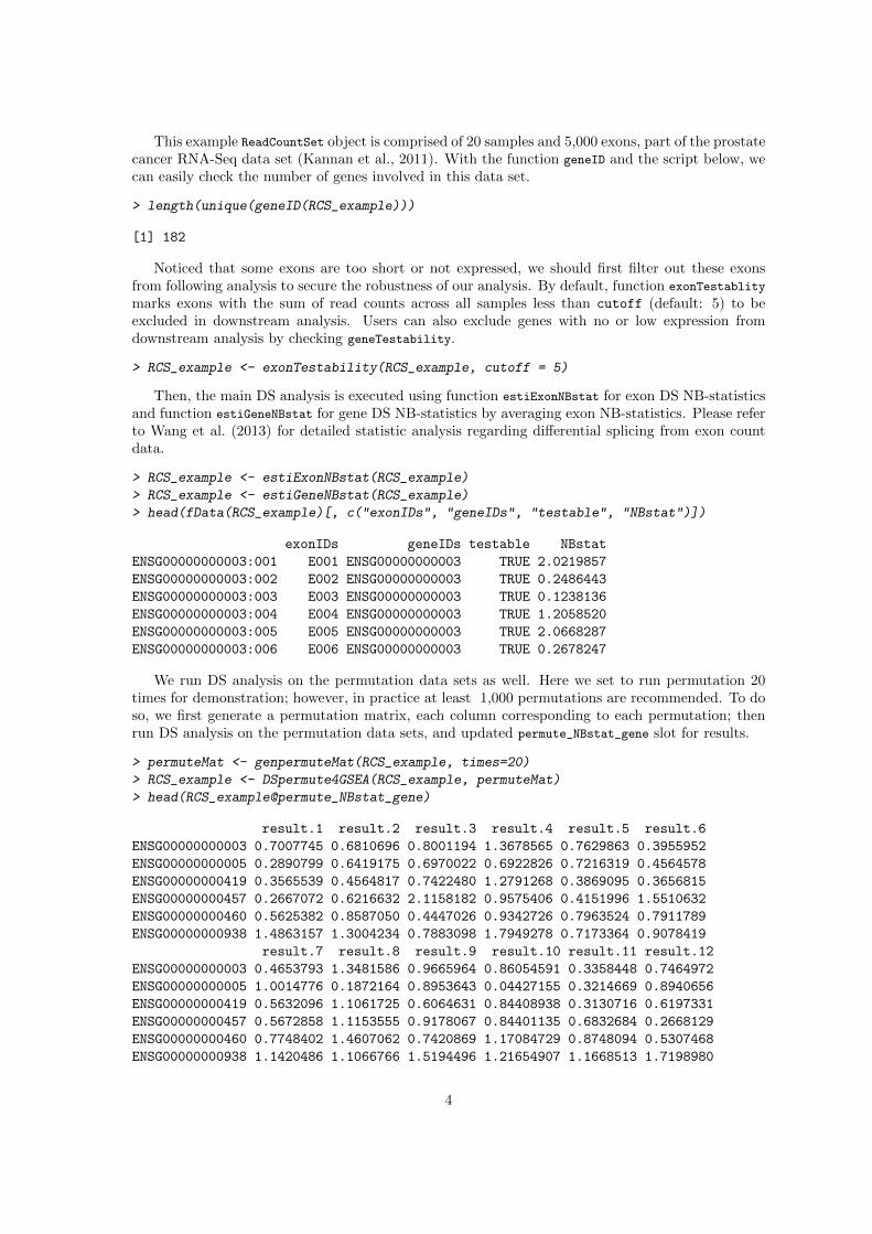
This example ReadCountSet object is comprised of 20 samples and 5,000 exons, part of the prostatecancer RNA-Seq data set (Kannan et al., 2011). With the function geneID and the script below, wecan easily check the number of genes involved in this data set.

> length(unique(geneID(RCS_example)))

[1] 182

Noticed that some exons are too short or not expressed, we should first filter out these exonsfrom following analysis to secure the robustness of our analysis. By default, function exonTestablity

marks exons with the sum of read counts across all samples less than cutoff (default: 5) to beexcluded in downstream analysis. Users can also exclude genes with no or low expression fromdownstream analysis by checking geneTestability.

> RCS_example <- exonTestability(RCS_example, cutoff = 5)

Then, the main DS analysis is executed using function estiExonNBstat for exon DS NB-statisticsand function estiGeneNBstat for gene DS NB-statistics by averaging exon NB-statistics. Please referto Wang et al. (2013) for detailed statistic analysis regarding differential splicing from exon countdata.

> RCS_example <- estiExonNBstat(RCS_example)

> RCS_example <- estiGeneNBstat(RCS_example)

> head(fData(RCS_example)[, c("exonIDs", "geneIDs", "testable", "NBstat")])

exonIDs geneIDs testable NBstat

ENSG00000000003:001 E001 ENSG00000000003 TRUE 2.0219857

ENSG00000000003:002 E002 ENSG00000000003 TRUE 0.2486443

ENSG00000000003:003 E003 ENSG00000000003 TRUE 0.1238136

ENSG00000000003:004 E004 ENSG00000000003 TRUE 1.2058520

ENSG00000000003:005 E005 ENSG00000000003 TRUE 2.0668287

ENSG00000000003:006 E006 ENSG00000000003 TRUE 0.2678247

We run DS analysis on the permutation data sets as well. Here we set to run permutation 20times for demonstration; however, in practice at least 1,000 permutations are recommended. To doso, we first generate a permutation matrix, each column corresponding to each permutation; thenrun DS analysis on the permutation data sets, and updated permute_NBstat_gene slot for results.

> permuteMat <- genpermuteMat(RCS_example, times=20)

> RCS_example <- DSpermute4GSEA(RCS_example, permuteMat)

> head(RCS_example@permute_NBstat_gene)

result.1 result.2 result.3 result.4 result.5 result.6

ENSG00000000003 0.7007745 0.6810696 0.8001194 1.3678565 0.7629863 0.3955952

ENSG00000000005 0.2890799 0.6419175 0.6970022 0.6922826 0.7216319 0.4564578

ENSG00000000419 0.3565539 0.4564817 0.7422480 1.2791268 0.3869095 0.3656815

ENSG00000000457 0.2667072 0.6216632 2.1158182 0.9575406 0.4151996 1.5510632

ENSG00000000460 0.5625382 0.8587050 0.4447026 0.9342726 0.7963524 0.7911789

ENSG00000000938 1.4863157 1.3004234 0.7883098 1.7949278 0.7173364 0.9078419


ENSG00000000003 0.4653793 1.3481586 0.9665964 0.86054591 0.3358448 0.7464972

ENSG00000000005 1.0014776 0.1872164 0.8953643 0.04427155 0.3214669 0.8940656

ENSG00000000419 0.5632096 1.1061725 0.6064631 0.84408938 0.3130716 0.6197331

ENSG00000000457 0.5672858 1.1153555 0.9178067 0.84401135 0.6832684 0.2668129

ENSG00000000460 0.7748402 1.4607062 0.7420869 1.17084729 0.8748094 0.5307468

ENSG00000000938 1.1420486 1.1066766 1.5194496 1.21654907 1.1668513 1.7198980

4


ENSG00000000003 0.2571302 1.6120477 1.3302056 1.0428132 1.0205647 1.0821191

ENSG00000000005 0.6758527 1.1252846 0.6081578 0.3410816 0.2647370 0.5409457

ENSG00000000419 0.6360393 2.7132621 0.8336165 0.8765478 1.1150284 0.9568325

ENSG00000000457 1.2055418 0.9339256 0.6039946 0.9060333 0.7336234 0.3441643

ENSG00000000460 0.5035748 1.1321705 0.5058564 1.1200971 0.5505624 0.9524635

ENSG00000000938 1.2530659 1.5170496 0.9797465 0.9537183 1.0271922 0.8803957

result.19 result.20

ENSG00000000003 0.7728963 0.5609182

ENSG00000000005 0.4502319 0.6175032

ENSG00000000419 0.4372623 0.6577665

ENSG00000000457 0.6968984 0.8511259

ENSG00000000460 0.5254690 0.4432378

ENSG00000000938 0.9736282 1.1694165

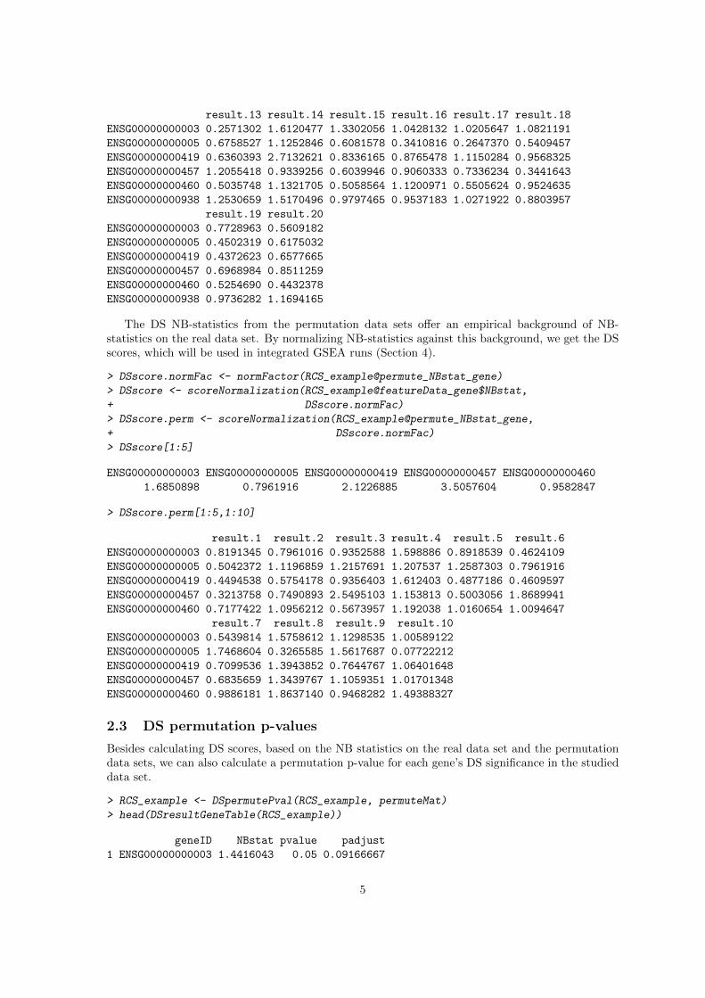
The DS NB-statistics from the permutation data sets offer an empirical background of NB-statistics on the real data set. By normalizing NB-statistics against this background, we get the DSscores, which will be used in integrated GSEA runs (Section 4).

> DSscore.normFac <- normFactor(RCS_example@permute_NBstat_gene)

> DSscore <- scoreNormalization(RCS_example@featureData_gene$NBstat,

+ DSscore.normFac)

> DSscore.perm <- scoreNormalization(RCS_example@permute_NBstat_gene,

+ DSscore.normFac)

> DSscore[1:5]

ENSG00000000003 ENSG00000000005 ENSG00000000419 ENSG00000000457 ENSG00000000460

1.6850898 0.7961916 2.1226885 3.5057604 0.9582847

> DSscore.perm[1:5,1:10]


ENSG00000000003 0.8191345 0.7961016 0.9352588 1.598886 0.8918539 0.4624109

ENSG00000000005 0.5042372 1.1196859 1.2157691 1.207537 1.2587303 0.7961916

ENSG00000000419 0.4494538 0.5754178 0.9356403 1.612403 0.4877186 0.4609597

ENSG00000000457 0.3213758 0.7490893 2.5495103 1.153813 0.5003056 1.8689941

ENSG00000000460 0.7177422 1.0956212 0.5673957 1.192038 1.0160654 1.0094647

result.7 result.8 result.9 result.10

ENSG00000000003 0.5439814 1.5758612 1.1298535 1.00589122

ENSG00000000005 1.7468604 0.3265585 1.5617687 0.07722212

ENSG00000000419 0.7099536 1.3943852 0.7644767 1.06401648

ENSG00000000457 0.6835659 1.3439767 1.1059351 1.01701348

ENSG00000000460 0.9886181 1.8637140 0.9468282 1.49388327

2.3 DS permutation p-values

Besides calculating DS scores, based on the NB statistics on the real data set and the permutationdata sets, we can also calculate a permutation p-value for each gene’s DS significance in the studieddata set.

> RCS_example <- DSpermutePval(RCS_example, permuteMat)

> head(DSresultGeneTable(RCS_example))

geneID NBstat pvalue padjust

1 ENSG00000000003 1.4416043 0.05 0.09166667

5

2 ENSG00000000005 0.4564578 0.65 0.67692308

3 ENSG00000000419 1.6839390 0.05 0.09166667

4 ENSG00000000457 2.9094026 0.00 0.00000000

5 ENSG00000000460 0.7510661 0.55 0.59753086

6 ENSG00000000938 1.7949049 0.05 0.09166667

The adjusted p-values accounting for multiple testings were given by the BH method (Benjaminiand Hochberg, 1995). Users can also apply function topDSGenes and function topDSExons to quicklyget the most significant DS genes and exons, respectively.

3 Differential expression analysis and DE scores

3.1 Gene read count data from ReadCountSet class

For gene DE analysis, read counts on each gene should be first calculated. With SeqGSEA, usersusually analyze DE and DS simultaneously, so the package includes the function getGeneCount tofacilitate gene read count calculation from a ReadCountSet object.

> geneCounts <- getGeneCount(RCS_example)

> dim(geneCounts) # 182 20

[1] 182 20

> head(geneCounts)

S1 S2 S3 S4 S5 S6 S7 S8 S9 S10 C1 C2 C3 C4 C5

ENSG00000000003 495 235 386 272 255 815 1065 803 839 885 278 270 238 175 292

ENSG00000000005 19 1 0 2 2 12 7 3 1 4 4 4 2 0 1

ENSG00000000419 196 134 165 184 132 344 343 307 342 280 179 156 100 120 126

ENSG00000000457 97 78 141 72 102 219 344 277 337 249 62 48 40 43 52

ENSG00000000460 52 35 48 25 47 105 124 80 156 145 48 36 21 34 19

ENSG00000000938 27 44 57 43 14 71 74 146 148 165 48 59 32 79 20

C6 C7 C8 C9 C10

ENSG00000000003 432 519 621 475 560

ENSG00000000005 9 3 1 14 46

ENSG00000000419 169 255 171 164 201

ENSG00000000457 170 165 131 183 185

ENSG00000000460 68 90 48 72 38

ENSG00000000938 103 1285 137 156 90

This function results in a matrix of 182 rows and 20 columns, corresponding to 182 genes and 20samples.

3.2 DE analysis and DE scores

DE analysis has been implemented in several R/Bioconductor packages, of which DESeq (Andersand Huber, 2010) is mainly utilized in SeqGSEA for DE analysis. With DESeq , we can modelcount data with negative binomial distributions for accounting biological variations and variousbiases introduced in RNA-Seq. Given the read count data on individual genes and sample groupinginformation, basic DE analysis based on DESeq including size factor estimation and dispersionestimation, is encapsulated in the function runDESeq.

> label <- label(RCS_example)

> DEG <- runDESeq(geneCounts, label)

6

The function runDESeq returns a CountDataSet object, which is defined in the DESeq package. The DEanalysis in the DESeq package continues with the output CountDataSet object and conducts negative-binomial-based statistical tests for DE genes (using nbinomTest or nbinomGLMTest). However, in thisSeqGSEA package, we define NB statistics to quantify each gene’s expression difference betweensample groups.

The NB statistics for DE can be achieved by the following scripts.

> DEGres <- DENBStat4GSEA(DEG)

> DEGres[1:5, "NBstat"]

[1] 0.5426504 0.2503510 0.0231052 14.3384053 1.4101270

Similarly, we run DE analysis on the permutation data sets as well. The permuteMat should be thesame as used in DS analysis on the permutation data sets.

> DEpermNBstat <- DENBStatPermut4GSEA(DEG, permuteMat)

> DEpermNBstat[1:5, 1:10]


[1,] 0.20001500 0.48885092 0.3505506 0.13481351 0.21284178 2.959739441

[2,] 0.03720485 0.15892291 0.3027288 1.70455956 0.07544249 0.121340175

[3,] 0.03703078 0.01966157 0.7773975 0.08648008 0.17168615 0.674063158

[4,] 3.57343091 0.00253457 0.6887122 0.47178223 0.06557296 2.330146501

[5,] 0.13210318 1.67283023 6.2685509 0.05679851 0.38283450 0.007560216


[1,] 0.0006705968 0.11418798 0.77928974 0.05684225

[2,] 0.0108104019 2.59501831 0.08274852 4.41038611

[3,] 0.8334211172 0.49193362 0.04939893 0.29824064

[4,] 0.7389625768 0.18827444 0.30792429 0.29847585

[5,] 0.0764985457 0.01092493 2.38606695 0.02997483

Once again, the DE NB-statistics from the permutation data sets offer an empirical background,so we can normalize NB-statistics against this background. By doing so, we get the DE scores, whichwill also be used in integrated GSEA runs (Section 4).

> DEscore.normFac <- normFactor(DEpermNBstat)

> DEscore <- scoreNormalization(DEGres$NBstat, DEscore.normFac)

> DEscore.perm <- scoreNormalization(DEpermNBstat, DEscore.normFac)

> DEscore[1:5]

[1] 0.69677163 0.17959135 0.03596578 17.44047532 1.13003434

> DEscore.perm[1:5, 1:10]


[1,] 0.25682240 0.627692275 0.4501124 0.17310266 0.27329219 3.800351991

[2,] 0.02668921 0.114004666 0.2171650 1.22277989 0.05411929 0.087044378

[3,] 0.05764246 0.030605388 1.2101044 0.13461571 0.26724831 1.049253167

[4,] 4.34653173 0.003082917 0.8377130 0.57385087 0.07975947 2.834266549

[5,] 0.10586361 1.340557017 5.0234326 0.04551666 0.30679233 0.006058535


[1,] 0.0008610568 0.146619159 1.00062028 0.07298634

[2,] 0.0077549312 1.861557836 0.05936033 3.16382694

[3,] 1.2973112926 0.765748590 0.07689484 0.46424423

[4,] 0.8988348637 0.229007043 0.37454276 0.36305019

[5,] 0.0613036880 0.008754919 1.91212398 0.02402095

7

3.3 DE permutation p-values

Similar to DS analysis, comparing NB-statistics on the real data set and those on the permutationdata sets, we can get permutation p-values for each gene’s DE significance.

> DEGres <- DEpermutePval(DEGres, DEpermNBstat)

> DEGres[1:6, c("NBstat", "perm.pval", "perm.padj")]

NBstat perm.pval perm.padj

ENSG00000000003 0.5426504 0.40 1

ENSG00000000005 0.2503510 0.55 1

ENSG00000000419 0.0231052 0.85 1

ENSG00000000457 14.3384053 0.00 0

ENSG00000000460 1.4101270 0.30 1

ENSG00000000938 2.1976989 0.00 0

For a comparison to the nominal p-values from exact testing and forming comprehensive results,users can run DENBTest first and then DEpermutePval, which generates results as follows.

> DEGres <- DENBTest(DEG)

> DEGres <- DEpermutePval(DEGres, DEpermNBstat)

> DEGres[1:6, c("NBstat", "pval", "padj", "perm.pval", "perm.padj")]

NBstat pval padj perm.pval perm.padj

ENSG00000000003 0.5426504 3.956985e-01 5.408276e-01 0.40 1

ENSG00000000005 0.2503510 3.300042e-01 4.943803e-01 0.55 1

ENSG00000000419 0.0231052 9.244775e-01 9.839468e-01 0.85 1

ENSG00000000457 14.3384053 9.960426e-05 2.589711e-03 0.00 0

ENSG00000000460 1.4101270 1.370959e-01 2.970412e-01 0.30 1

ENSG00000000938 2.1976989 7.309013e-07 4.434134e-05 0.00 0

4 Integrative GSEA runs

4.1 DE/DS score integration

We have proposed two strategies for integrating normalized DE and DS scores (Wang and Cairns,2013), one of which is the weighted summation of the two scores and the other is a rank-basedstrategy. The functions geneScore and genePermuteScore implement two methods for the weightedsummation strategy: weighted linear combination and weighted quadratic combination. Scriptsbelow show a linear combination of DE and DS scores with weight for DE equal to 0.3. Users shouldkeep the weight for DE in geneScore and genePermuteScore the same, and the weight rangs from0 (i.e., DS only) to 1 (i.e., DE only). Visualization of gene scores can be made by applying theplotGeneScore function.

> gene.score <- geneScore(DEscore, DSscore, method="linear", DEweight = 0.3)

> gene.score.perm <- genePermuteScore(DEscore.perm, DSscore.perm,

+ method="linear", DEweight=0.3)

> plotGeneScore(gene.score, gene.score.perm)

The plot generated by the plotGeneScore function (Fig. 1) can also be saved as a PDF file easilywith the pdf argument of plotGeneScore.

The functions geneScore and genePermuteScore also implement one method for the rank-basedintegration strategy: using data-set-specific ranks. The plot for integrated gene scores is shown inFig. 2.

8

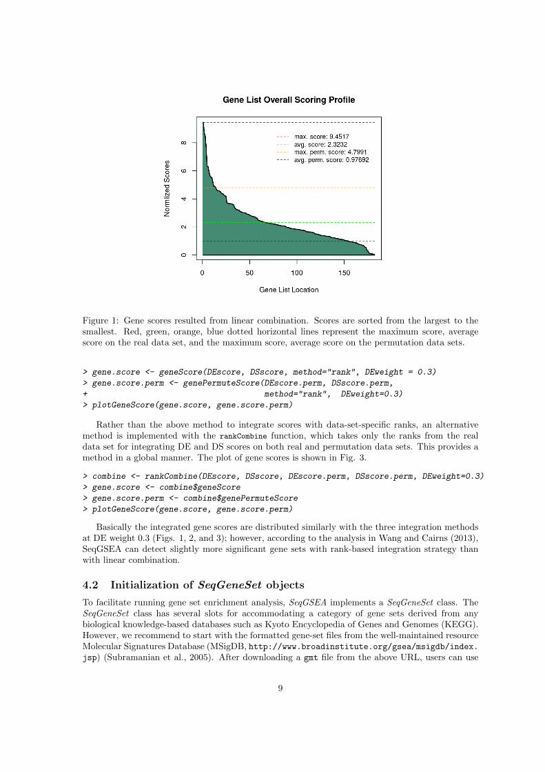
Figure 1: Gene scores resulted from linear combination. Scores are sorted from the largest to thesmallest. Red, green, orange, blue dotted horizontal lines represent the maximum score, averagescore on the real data set, and the maximum score, average score on the permutation data sets.

> gene.score <- geneScore(DEscore, DSscore, method="rank", DEweight = 0.3)

> gene.score.perm <- genePermuteScore(DEscore.perm, DSscore.perm,

+ method="rank", DEweight=0.3)


Rather than the above method to integrate scores with data-set-specific ranks, an alternativemethod is implemented with the rankCombine function, which takes only the ranks from the realdata set for integrating DE and DS scores on both real and permutation data sets. This provides amethod in a global manner. The plot of gene scores is shown in Fig. 3.

> combine <- rankCombine(DEscore, DSscore, DEscore.perm, DSscore.perm, DEweight=0.3)

> gene.score <- combine$geneScore

> gene.score.perm <- combine$genePermuteScore


Basically the integrated gene scores are distributed similarly with the three integration methodsat DE weight 0.3 (Figs. 1, 2, and 3); however, according to the analysis in Wang and Cairns (2013),SeqGSEA can detect slightly more significant gene sets with rank-based integration strategy thanwith linear combination.

4.2 Initialization of SeqGeneSet objects

To facilitate running gene set enrichment analysis, SeqGSEA implements a SeqGeneSet class. TheSeqGeneSet class has several slots for accommodating a category of gene sets derived from anybiological knowledge-based databases such as Kyoto Encyclopedia of Genes and Genomes (KEGG).However, we recommend to start with the formatted gene-set files from the well-maintained resourceMolecular Signatures Database (MSigDB, http://www.broadinstitute.org/gsea/msigdb/index.jsp) (Subramanian et al., 2005). After downloading a gmt file from the above URL, users can use

9

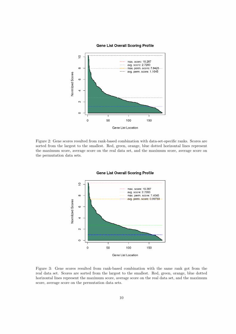
http://www.broadinstitute.org/gsea/msigdb/index.jsp


Figure 2: Gene scores resulted from rank-based combination with data-set-specific ranks. Scores aresorted from the largest to the smallest. Red, green, orange, blue dotted horizontal lines representthe maximum score, average score on the real data set, and the maximum score, average score onthe permutation data sets.

Figure 3: Gene scores resulted from rank-based combination with the same rank got from thereal data set. Scores are sorted from the largest to the smallest. Red, green, orange, blue dottedhorizontal lines represent the maximum score, average score on the real data set, and the maximumscore, average score on the permutation data sets.

10

loadGenesets to initialize a SeqGeneSet object easily. Please note that with the current version ofSeqGSEA, only gene sets with gene symbols are supported, though read count data’s gene IDs canbe either gene symbols or Ensembl Gene IDs.

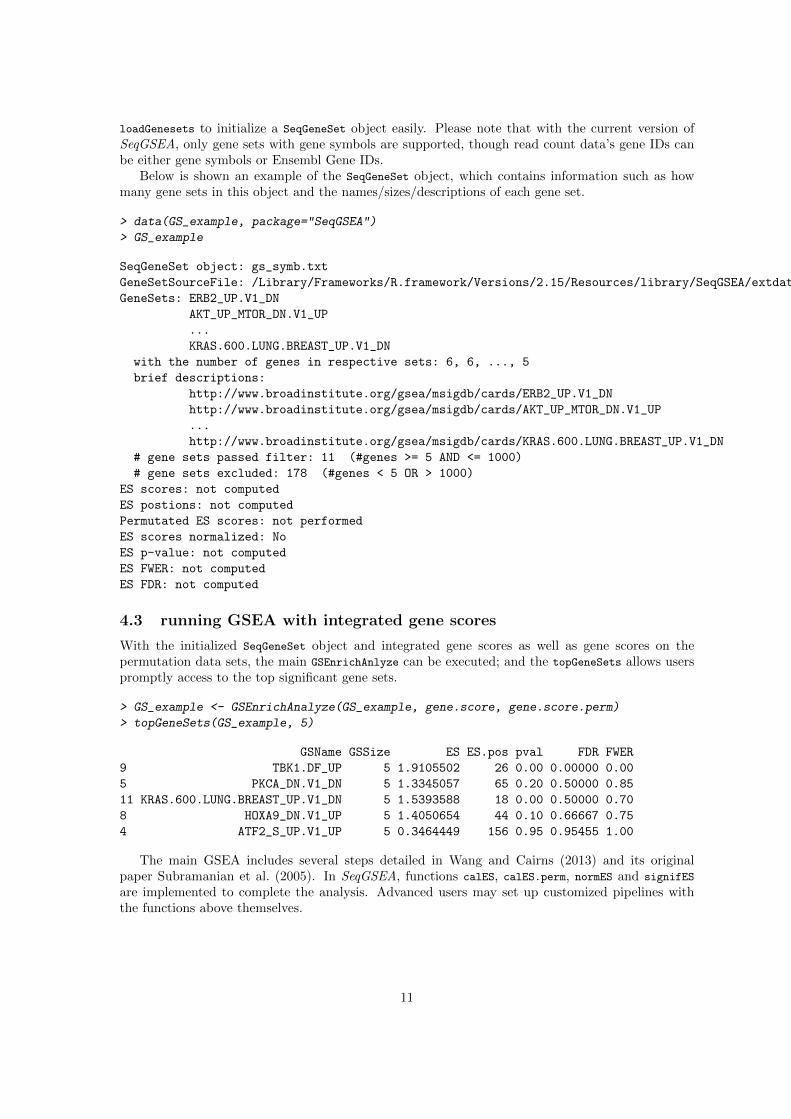
Below is shown an example of the SeqGeneSet object, which contains information such as howmany gene sets in this object and the names/sizes/descriptions of each gene set.

> data(GS_example, package="SeqGSEA")

> GS_example

SeqGeneSet object: gs_symb.txt

GeneSetSourceFile: /Library/Frameworks/R.framework/Versions/2.15/Resources/library/SeqGSEA/extdata/gs_symb.txt

GeneSets: ERB2_UP.V1_DN

AKT_UP_MTOR_DN.V1_UP

...

KRAS.600.LUNG.BREAST_UP.V1_DN

with the number of genes in respective sets: 6, 6, ..., 5

brief descriptions:

http://www.broadinstitute.org/gsea/msigdb/cards/ERB2_UP.V1_DN

http://www.broadinstitute.org/gsea/msigdb/cards/AKT_UP_MTOR_DN.V1_UP

...

http://www.broadinstitute.org/gsea/msigdb/cards/KRAS.600.LUNG.BREAST_UP.V1_DN

# gene sets passed filter: 11 (#genes >= 5 AND <= 1000)

# gene sets excluded: 178 (#genes < 5 OR > 1000)

ES scores: not computed

ES postions: not computed

Permutated ES scores: not performed

ES scores normalized: No

ES p-value: not computed

ES FWER: not computed

ES FDR: not computed

4.3 running GSEA with integrated gene scores

With the initialized SeqGeneSet object and integrated gene scores as well as gene scores on thepermutation data sets, the main GSEnrichAnlyze can be executed; and the topGeneSets allows userspromptly access to the top significant gene sets.

> GS_example <- GSEnrichAnalyze(GS_example, gene.score, gene.score.perm)

> topGeneSets(GS_example, 5)

GSName GSSize ES ES.pos pval FDR FWER

9 TBK1.DF_UP 5 1.9105502 26 0.00 0.00000 0.00

5 PKCA_DN.V1_DN 5 1.3345057 65 0.20 0.50000 0.85

11 KRAS.600.LUNG.BREAST_UP.V1_DN 5 1.5393588 18 0.00 0.50000 0.70

8 HOXA9_DN.V1_UP 5 1.4050654 44 0.10 0.66667 0.75

4 ATF2_S_UP.V1_UP 5 0.3464449 156 0.95 0.95455 1.00

The main GSEA includes several steps detailed in Wang and Cairns (2013) and its originalpaper Subramanian et al. (2005). In SeqGSEA, functions calES, calES.perm, normES and signifES

are implemented to complete the analysis. Advanced users may set up customized pipelines withthe functions above themselves.

11

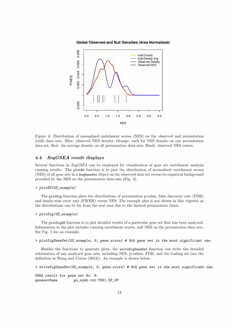
Figure 4: Distribution of normalized enrichment scores (NES) on the observed and permutation(null) data sets. Blue: observed NES density; Orange: each for NES density on one permutationdata set; Red: the average density on all permutation data sets; Black: observed NES values.

4.4 SeqGSEA result displays

Several functions in SeqGSEA can be employed for visualization of gene set enrichment analysisrunning results. The plotES function is to plot the distribution of normalized enrichment scores(NES) of all gene sets in a SeqGeneSet object on the observed data set versus its empirical backgroundprovided by the NES on the permutation data sets (Fig. 4).

> plotES(GS_example)

The plotSig function plots the distributions of permutation p-value, false discovery rate (FDR)and family-wise error rate (FWER) versus NES. The example plot is not shown in this vignette asthe distributions can be far from the real ones due to the limited permutation times.

> plotSig(GS_example)

The plotSigGS function is to plot detailed results of a particular gene set that has been analyzed.Information in the plot includes running enrichment scores, null NES on the permutation data sets.See Fig. 5 for an example.

> plotSigGeneSet(GS_example, 9, gene.score) # 9th gene set is the most significant one.

Besides the functions to generate plots, the writeSigGeneSet function can write the detailedinformation of any analyzed gene sets, including NES, p-values, FDR, and the leading set (see thedefinition in Wang and Cairns (2013)). An example is shown below.

> writeSigGeneSet(GS_example, 9, gene.score) # 9th gene set is the most significant one.

GSEA result for gene set No. 9:

genesetName gs_symb.txt:TBK1.DF_UP

12

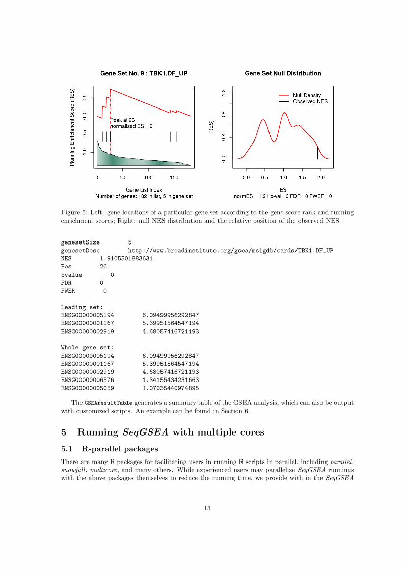
Figure 5: Left: gene locations of a particular gene set according to the gene score rank and runningenrichment scores; Right: null NES distribution and the relative position of the observed NES.

genesetSize 5

genesetDesc http://www.broadinstitute.org/gsea/msigdb/cards/TBK1.DF_UP

NES 1.9105501883631

Pos 26

pvalue 0

FDR 0

FWER 0

Leading set:

ENSG00000005194 6.09499956292847

ENSG00000001167 5.39951564547194

ENSG00000002919 4.68057416721193

Whole gene set:

ENSG00000005194 6.09499956292847

ENSG00000001167 5.39951564547194

ENSG00000002919 4.68057416721193

ENSG00000006576 1.34155434231663

ENSG00000005059 1.07035440974895

The GSEAresultTable generates a summary table of the GSEA analysis, which can also be outputwith customized scripts. An example can be found in Section 6.

5 Running SeqGSEA with multiple cores

5.1 R-parallel packages

There are many R packages for facilitating users in running R scripts in parallel, including parallel ,snowfall , multicore, and many others. While experienced users may parallelize SeqGSEA runningswith the above packages themselves to reduce the running time, we provide with in the SeqGSEA

13

package vignette an general way for users to parallelize their runnings utilizing the doParallel package(which depends on parallel).

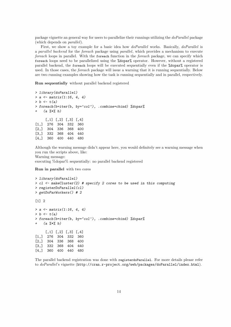
First, we show a toy example for a basic idea how doParallel works. Basically, doParallel isa parallel backend for the foreach package using parallel , which provides a mechanism to executeforeach loops in parallel. With the foreach function in the foreach package, we can specify whichforeach loops need to be parallelized using the %dopar% operator. However, without a registeredparallel backend, the foreach loops will be executed sequentially even if the %dopar% operator isused. In those cases, the foreach package will issue a warning that it is running sequentially. Beloware two running examples showing how the task is running sequentially and in parallel, respectively.

Run sequentially without parallel backend registered

> library(doParallel)

> a <- matrix(1:16, 4, 4)

> b <- t(a)

> foreach(b=iter(b, by='col'), .combine=cbind) %dopar%

+ (a %*% b)

[,1] [,2] [,3] [,4]

[1,] 276 304 332 360

[2,] 304 336 368 400

[3,] 332 368 404 440

[4,] 360 400 440 480

Although the warning message didn’t appear here, you would definitely see a warning message whenyou run the scripts above, like:Warning message:executing %dopar% sequentially: no parallel backend registered

Run in parallel with two cores


> cl <- makeCluster(2) # specify 2 cores to be used in this computing

> registerDoParallel(cl)

> getDoParWorkers() # 2

[1] 2

> a <- matrix(1:16, 4, 4)

> b <- t(a)

> foreach(b=iter(b, by='col'), .combine=cbind) %dopar%

+ (a %*% b)

[,1] [,2] [,3] [,4]

[1,] 276 304 332 360

[2,] 304 336 368 400

[3,] 332 368 404 440

[4,] 360 400 440 480

The parallel backend registration was done with registerdoParallel. For more details please referto doParallel ’s vignette (http://cran.r-project.org/web/packages/doParallel/index.html).

14

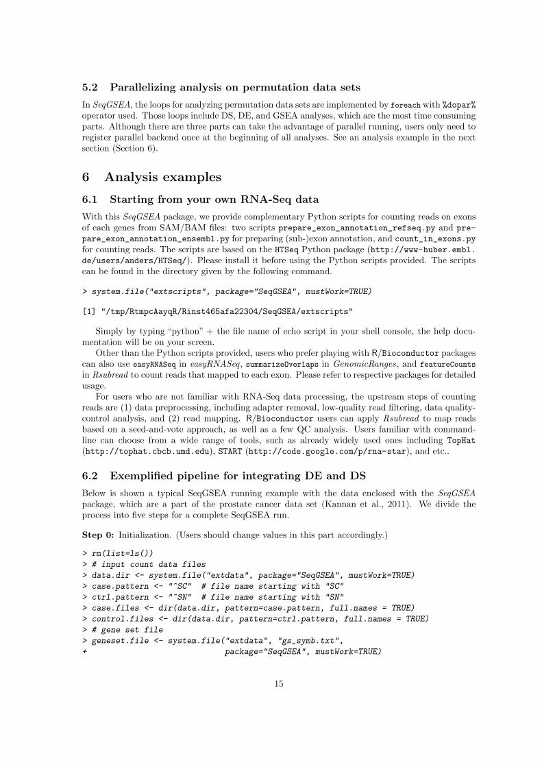
http://cran.r-project.org/web/packages/doParallel/index.html

5.2 Parallelizing analysis on permutation data sets

In SeqGSEA, the loops for analyzing permutation data sets are implemented by foreach with %dopar%

operator used. Those loops include DS, DE, and GSEA analyses, which are the most time consumingparts. Although there are three parts can take the advantage of parallel running, users only need toregister parallel backend once at the beginning of all analyses. See an analysis example in the nextsection (Section 6).

6 Analysis examples

6.1 Starting from your own RNA-Seq data

With this SeqGSEA package, we provide complementary Python scripts for counting reads on exonsof each genes from SAM/BAM files: two scripts prepare_exon_annotation_refseq.py and pre-

pare_exon_annotation_ensembl.py for preparing (sub-)exon annotation, and count_in_exons.py

for counting reads. The scripts are based on the HTSeq Python package (http://www-huber.embl.de/users/anders/HTSeq/). Please install it before using the Python scripts provided. The scriptscan be found in the directory given by the following command.

> system.file("extscripts", package="SeqGSEA", mustWork=TRUE)

[1] "/tmp/RtmpcAayqR/Rinst465afa22304/SeqGSEA/extscripts"

Simply by typing “python” + the file name of echo script in your shell console, the help docu-mentation will be on your screen.

Other than the Python scripts provided, users who prefer playing with R/Bioconductor packagescan also use easyRNASeq in easyRNASeq , summarizeOverlaps in GenomicRanges, and featureCounts

in Rsubread to count reads that mapped to each exon. Please refer to respective packages for detailedusage.

For users who are not familiar with RNA-Seq data processing, the upstream steps of countingreads are (1) data preprocessing, including adapter removal, low-quality read filtering, data quality-control analysis, and (2) read mapping. R/Bioconductor users can apply Rsubread to map readsbased on a seed-and-vote approach, as well as a few QC analysis. Users familiar with command-line can choose from a wide range of tools, such as already widely used ones including TopHat

(http://tophat.cbcb.umd.edu), START (http://code.google.com/p/rna-star), and etc..

6.2 Exemplified pipeline for integrating DE and DS

Below is shown a typical SeqGSEA running example with the data enclosed with the SeqGSEApackage, which are a part of the prostate cancer data set (Kannan et al., 2011). We divide theprocess into five steps for a complete SeqGSEA run.

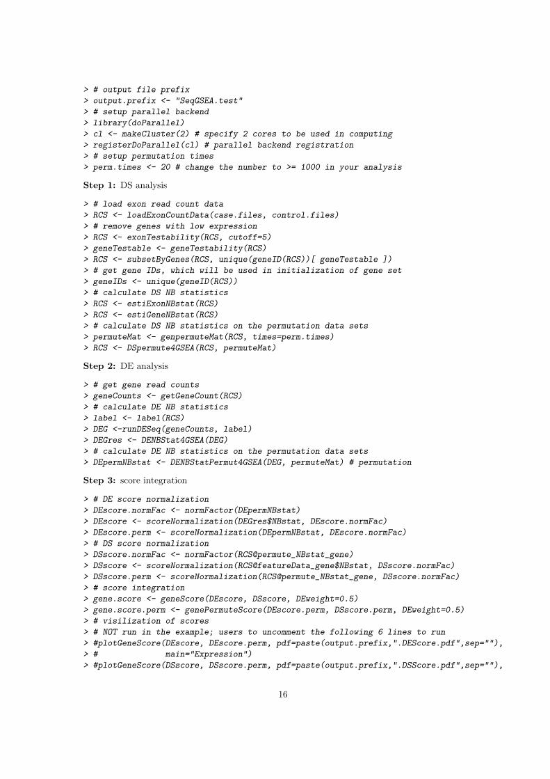
Step 0: Initialization. (Users should change values in this part accordingly.)

> rm(list=ls())

> # input count data files

> data.dir <- system.file("extdata", package="SeqGSEA", mustWork=TRUE)

> case.pattern <- "^SC" # file name starting with "SC"

> ctrl.pattern <- "^SN" # file name starting with "SN"

> case.files <- dir(data.dir, pattern=case.pattern, full.names = TRUE)

> control.files <- dir(data.dir, pattern=ctrl.pattern, full.names = TRUE)

> # gene set file

> geneset.file <- system.file("extdata", "gs_symb.txt",

+ package="SeqGSEA", mustWork=TRUE)

15

http://www-huber.embl.de/users/anders/HTSeq/

http://www-huber.embl.de/users/anders/HTSeq/

http://tophat.cbcb.umd.edu

http://code.google.com/p/rna-star

> # output file prefix

> output.prefix <- "SeqGSEA.test"

> # setup parallel backend


> cl <- makeCluster(2) # specify 2 cores to be used in computing

> registerDoParallel(cl) # parallel backend registration

> # setup permutation times

> perm.times <- 20 # change the number to >= 1000 in your analysis

Step 1: DS analysis

> # load exon read count data

> RCS <- loadExonCountData(case.files, control.files)

> # remove genes with low expression

> RCS <- exonTestability(RCS, cutoff=5)

> geneTestable <- geneTestability(RCS)

> RCS <- subsetByGenes(RCS, unique(geneID(RCS))[ geneTestable ])

> # get gene IDs, which will be used in initialization of gene set

> geneIDs <- unique(geneID(RCS))

> # calculate DS NB statistics

> RCS <- estiExonNBstat(RCS)

> RCS <- estiGeneNBstat(RCS)

> # calculate DS NB statistics on the permutation data sets

> permuteMat <- genpermuteMat(RCS, times=perm.times)

> RCS <- DSpermute4GSEA(RCS, permuteMat)

Step 2: DE analysis

> # get gene read counts

> geneCounts <- getGeneCount(RCS)

> # calculate DE NB statistics

> label <- label(RCS)

> DEG <-runDESeq(geneCounts, label)


> # calculate DE NB statistics on the permutation data sets

> DEpermNBstat <- DENBStatPermut4GSEA(DEG, permuteMat) # permutation

Step 3: score integration

> # DE score normalization




> # DS score normalization

> DSscore.normFac <- normFactor(RCS@permute_NBstat_gene)

> DSscore <- scoreNormalization(RCS@featureData_gene$NBstat, DSscore.normFac)

> DSscore.perm <- scoreNormalization(RCS@permute_NBstat_gene, DSscore.normFac)

> # score integration

> gene.score <- geneScore(DEscore, DSscore, DEweight=0.5)

> gene.score.perm <- genePermuteScore(DEscore.perm, DSscore.perm, DEweight=0.5)

> # visilization of scores

> # NOT run in the example; users to uncomment the following 6 lines to run

> #plotGeneScore(DEscore, DEscore.perm, pdf=paste(output.prefix,".DEScore.pdf",sep=""),

> # main="Expression")

> #plotGeneScore(DSscore, DSscore.perm, pdf=paste(output.prefix,".DSScore.pdf",sep=""),

16

> # main="Splicing")

> #plotGeneScore(gene.score, gene.score.perm,

> # pdf=paste(output.prefix,".GeneScore.pdf",sep=""))

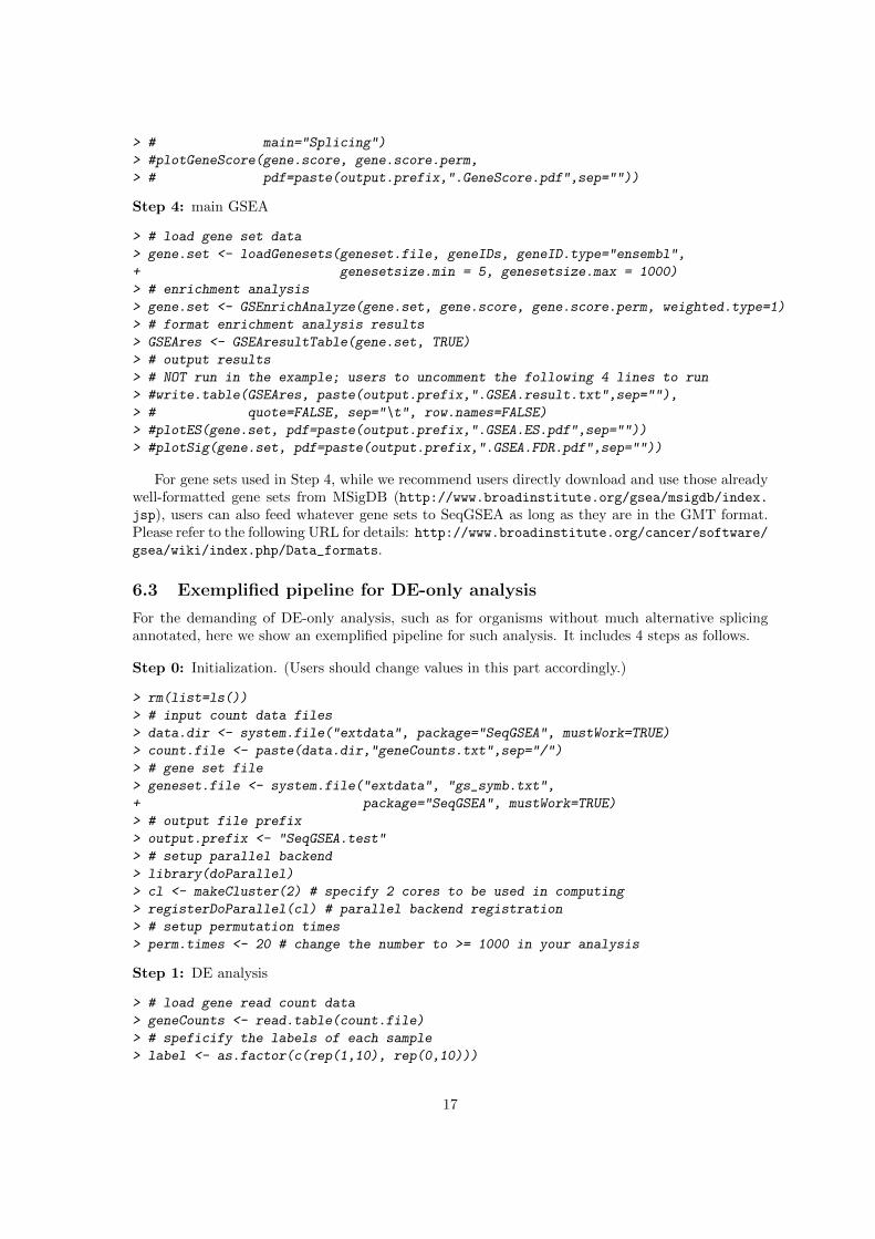
Step 4: main GSEA

> # load gene set data

> gene.set <- loadGenesets(geneset.file, geneIDs, geneID.type="ensembl",

+ genesetsize.min = 5, genesetsize.max = 1000)

> # enrichment analysis

> gene.set <- GSEnrichAnalyze(gene.set, gene.score, gene.score.perm, weighted.type=1)

> # format enrichment analysis results

> GSEAres <- GSEAresultTable(gene.set, TRUE)

> # output results


> #write.table(GSEAres, paste(output.prefix,".GSEA.result.txt",sep=""),

> # quote=FALSE, sep="\t", row.names=FALSE)

> #plotES(gene.set, pdf=paste(output.prefix,".GSEA.ES.pdf",sep=""))

> #plotSig(gene.set, pdf=paste(output.prefix,".GSEA.FDR.pdf",sep=""))

For gene sets used in Step 4, while we recommend users directly download and use those alreadywell-formatted gene sets from MSigDB (http://www.broadinstitute.org/gsea/msigdb/index.jsp), users can also feed whatever gene sets to SeqGSEA as long as they are in the GMT format.Please refer to the following URL for details: http://www.broadinstitute.org/cancer/software/gsea/wiki/index.php/Data_formats.

6.3 Exemplified pipeline for DE-only analysis

For the demanding of DE-only analysis, such as for organisms without much alternative splicingannotated, here we show an exemplified pipeline for such analysis. It includes 4 steps as follows.

Step 0: Initialization. (Users should change values in this part accordingly.)

> rm(list=ls())

> # input count data files


> count.file <- paste(data.dir,"geneCounts.txt",sep="/")

> # gene set file




> output.prefix <- "SeqGSEA.test"

> # setup parallel backend


> cl <- makeCluster(2) # specify 2 cores to be used in computing

> registerDoParallel(cl) # parallel backend registration

> # setup permutation times

> perm.times <- 20 # change the number to >= 1000 in your analysis

Step 1: DE analysis

> # load gene read count data

> geneCounts <- read.table(count.file)

> # speficify the labels of each sample

> label <- as.factor(c(rep(1,10), rep(0,10)))

17



http://www.broadinstitute.org/cancer/software/gsea/wiki/index.php/Data_formats

http://www.broadinstitute.org/cancer/software/gsea/wiki/index.php/Data_formats

> # calculate DE NB statistics

> DEG <-runDESeq(geneCounts, label)


> # calculate DE NB statistics on the permutation data sets

> permuteMat <- genpermuteMat(label, times=perm.times)

> DEpermNBstat <- DENBStatPermut4GSEA(DEG, permuteMat) # permutation

Step 2: score normalization

> # DE score normalization




> # score integration - DSscore can be null

> gene.score <- geneScore(DEscore, DEweight=1)

> gene.score.perm <- genePermuteScore(DEscore.perm, DEweight=1) # visilization of scores


> #plotGeneScore(DEscore, DEscore.perm, pdf=paste(output.prefix,".DEScore.pdf",sep=""),

> # main="Expression")

> #plotGeneScore(gene.score, gene.score.perm,

> # pdf=paste(output.prefix,".GeneScore.pdf",sep=""))

Step 3: main GSEA

> # load gene set data

> geneIDs <- rownames(geneCounts)

> gene.set <- loadGenesets(geneset.file, geneIDs, geneID.type="ensembl",

+ genesetsize.min = 5, genesetsize.max = 1000)

> # enrichment analysis

> gene.set <- GSEnrichAnalyze(gene.set, gene.score, gene.score.perm, weighted.type=1)

> # format enrichment analysis results

> GSEAres <- GSEAresultTable(gene.set, TRUE)

> # output results


> #write.table(GSEAres, paste(output.prefix,".GSEA.result.txt",sep=""),

> # quote=FALSE, sep="\t", row.names=FALSE)

> #plotES(gene.set, pdf=paste(output.prefix,".GSEA.ES.pdf",sep=""))

> #plotSig(gene.set, pdf=paste(output.prefix,".GSEA.FDR.pdf",sep=""))

6.4 One-step SeqGSEA analysis

While users can choose to run SeqGSEA step by step in a well-controlled manner (see above), theone-step SeqGSEA analysis with an all-in runSeqGSEA function enables users to run SeqGSEA inthe easiest way. With the runSeqGSEA function, users can also test multiple weights for integratingDE and DS scores. DE-only analysis starting with exon read counts is also supported in the all-infunction.

Follow the example below to start your first SeqGSEA analysis now!

> ### Initialization ###

> # input file location and pattern


> case.pattern <- "^SC" # file name starting with "SC"

> ctrl.pattern <- "^SN" # file name starting with "SN"

> # gene set file and type


18


> geneID.type <- "ensembl"


> output.prefix <- "SeqGSEA.example"

> # analysis parameters

> nCores <- 8

> perm.times <- 1000 # >= 1000 recommended

> DEonly <- FALSE

> DEweight <- c(0.2, 0.5, 0.8) # a vector for different weights

> integrationMethod <- "linear"

>

> ### one step SeqGSEA running ###

> # NOT run in the example; uncomment the following 4 lines to run

> # CAUTION: running the following lines will generate lots of files in your working dir

> #runSeqGSEA(data.dir=data.dir, case.pattern=case.pattern, ctrl.pattern=ctrl.pattern,

> # geneset.file=geneset.file, geneID.type=geneID.type, output.prefix=output.prefix,

> # nCores=nCores, perm.times=perm.times, integrationMethod=integrationMethod,

> # DEonly=DEonly, DEweight=DEweight)

7 Session information

> sessionInfo()

R version 3.3.1 (2016-06-21)

Platform: x86_64-pc-linux-gnu (64-bit)

Running under: Ubuntu 16.04.1 LTS

locale:

[1] LC_CTYPE=en_US.UTF-8 LC_NUMERIC=C

[3] LC_TIME=en_US.UTF-8 LC_COLLATE=C

[5] LC_MONETARY=en_US.UTF-8 LC_MESSAGES=en_US.UTF-8

[7] LC_PAPER=en_US.UTF-8 LC_NAME=C

[9] LC_ADDRESS=C LC_TELEPHONE=C

[11] LC_MEASUREMENT=en_US.UTF-8 LC_IDENTIFICATION=C

attached base packages:

[1] parallel stats graphics grDevices utils datasets methods

[8] base

other attached packages:

[1] SeqGSEA_1.14.0 DESeq_1.26.0 lattice_0.20-34

[4] locfit_1.5-9.1 doParallel_1.0.10 iterators_1.0.8

[7] foreach_1.4.3 Biobase_2.34.0 BiocGenerics_0.20.0

loaded via a namespace (and not attached):

[1] AnnotationDbi_1.36.0 splines_3.3.1 IRanges_2.8.0

[4] xtable_1.8-2 tools_3.3.1 grid_3.3.1

[7] DBI_0.5-1 genefilter_1.56.0 survival_2.39-5

[10] Matrix_1.2-7.1 RColorBrewer_1.1-2 geneplotter_1.52.0

[13] S4Vectors_0.12.0 bitops_1.0-6 codetools_0.2-15

[16] biomaRt_2.30.0 RCurl_1.95-4.8 RSQLite_1.0.0

[19] compiler_3.3.1 stats4_3.3.1 XML_3.98-1.4

[22] annotate_1.52.0

19

Cleanup

This is a cleanup step for the vignette on Windows; typically not needed for users.

> allCon <- showConnections()

> socketCon <- as.integer(rownames(allCon)[allCon[, "class"] == "sockconn"])

> sapply(socketCon, function(ii) close.connection(getConnection(ii)) )

References

Anders, S. and Huber, W. (2010). Differential expression analysis for sequence count data. GenomeBiology, 11:R106.

Benjamini, Y. and Hochberg, Y. (1995). Controlling the false discovery rate: a practical and powerfulapproach to multiple testing. J. R. Stat. Soc. Ser. B, 57(1):289–300.

Kannan, K., Wang, L., Wang, J., Ittmann, M. M., Li, W., and Yen, L. (2011). Recurrent chimericrnas enriched in human prostate cancer identified by deep sequencing. Proc Natl Acad Sci U S A,108(22):9172–7.

Subramanian, A., Tamayo, P., Mootha, V. K., Mukherjee, S., Ebert, B. L., Gillette, M. A., Paulovich,A., Pomeroy, S. L., Golub, T. R., Lander, E. S., and Mesirov, J. P. (2005). Gene set enrichmentanalysis: a knowledge-based approach for interpreting genome-wide expression profiles. Proc NatlAcad Sci U S A, 102(43):15545–50.

Wang, W., Qin, Z., Feng, Z., Wang, X., and Zhang, X. (2013). Identifying differentially spliced genesfrom two groups of rna-seq samples. Gene, 518(1):164–170.

Wang, X. and Cairns, M. (2013). Gene set enrichment analysis of RNA-Seq data: integratingdifferential expression and splicing. BMC Bioinformatics, 14(Suppl 5):S16.

Wang, X. and Cairns, M. (2014). SeqGSEA: a Bioconductor package for gene set enrichment analysisof RNA-Seq data integrating differential expression and splicing. Bioinformatics, 30(12):1777–9.

20

Gene set enrichment analysis of RNA-Seq data with …...Gene set enrichment analysis of RNA-Seq data...

Documents

Transcript of Gene set enrichment analysis of RNA-Seq data with …...Gene set enrichment analysis of RNA-Seq data...