Policy Research Working Paper 6066

Gender and Rural Non-farm EntrepreneurshipBob RijkersRita Costa

The World BankDevelopment Research GroupMacroeconomics and Growth TeamMay 2012

WPS6066P

ublic

Dis

clos

ure

Aut

horiz

edP

ublic

Dis

clos

ure

Aut

horiz

edP

ublic

Dis

clos

ure

Aut

horiz

edP

ublic

Dis

clos

ure

Aut

horiz

edP

ublic

Dis

clos

ure

Aut

horiz

edP

ublic

Dis

clos

ure

Aut

horiz

edP

ublic

Dis

clos

ure

Aut

horiz

edP

ublic

Dis

clos

ure

Aut

horiz

ed

Produced by the Research Support Team

Abstract

The Policy Research Working Paper Series disseminates the findings of work in progress to encourage the exchange of ideas about development issues. An objective of the series is to get the findings out quickly, even if the presentations are less than fully polished. The papers carry the names of the authors and should be cited accordingly. The findings, interpretations, and conclusions expressed in this paper are entirely those of the authors. They do not necessarily represent the views of the International Bank for Reconstruction and Development/World Bank and its affiliated organizations, or those of the Executive Directors of the World Bank or the governments they represent.

Policy Research Working Paper 6066

Despite their increasing prominence in policy debates, little is known about gender inequities in non-agricultural labor market outcomes in rural areas. Using matched household-enterprise-community data sets from Bangladesh, Ethiopia, Indonesia and Sri Lanka, this paper documents and analyzes gender differences in the individual portfolio choice and productivity of non-farm entrepreneurship. Except for Ethiopia, women are less likely than men to become nonfarm entrepreneurs. Women’s nonfarm entrepreneurship isn’t strongly correlated with household composition or educational attainment, but is especially prevalent amongst women who are the head of their household. Female-led firms

This paper is a product of the Macroeconomics and Growth Team, Development Research Group. It is part of a larger effort by the World Bank to provide open access to its research and make a contribution to development policy discussions around the world. Policy Research Working Papers are also posted on the Web at http://econ.worldbank.org. The author may be contacted at brijkers@worldbank.org.

are much smaller and less productive on average, though gender differences in productivity vary dramatically across countries. Mean differences in log output per worker suggest that male firms are roughly 10 times as productive as female firms in Bangladesh, three times as those in Ethiopia and twice as those in Sri Lanka. By contrast, no significant differences in labor productivity were detected in Indonesia. Differences in output per worker are overwhelmingly accounted for by sorting by sector and size. They can’t be explained by differences in capital intensity, human capital or the local investment climate, nor by increasing returns to scale.

Gender and Rural Non-farm Entrepreneurship

Bob Rijkers1 Rita Costa2

Key words: gender, entrepreneurship, rural, Indonesia, Bangladesh, Sri Lanka, Ethiopia

JEL codes: D13, D22, J21, J24, L25, L26, R30

Acknowledgements

We would like to thank Klaus Deininger, Donald Larson, Josef Loening, Jack Molyneaux, Naotaka

Sawada, and Mona Sur for their help in obtaining the data, and seminar participants at the 2011

World Bank Economists’ forum, Reena Badiani, Liang Choon Wang, Mary Hallward-Driemeier,

Andrew Mason, Luis Serven, and especially Carolina Sanchez Paramo for helpful discussions and

critical feedback. The views expressed here are those of the authors and do not necessarily represent

the views of the World Bank, its Executive Board or member countries. All errors are our own.

1 MNACE, EPOL

2 HDNED, EDU

2

1. INTRODUCTION

The potentially deleterious effects of gender disparities on growth and poverty reduction

have been receiving progressively more policy attention, reflected, for instance, in the inclusion of

the promotion of gender parity among the Millennium Development Goals and the 2012 World

Development Report on Gender Equity. Inequities in labor market opportunities are of particular

concern since labor earnings are the most important source of income for the poor in the vast

majority of developing countries (Lustig, 2000). Women’s over-representation in poverty has been

attributed to their lack of labor market opportunities (see e.g. Buvinic and Gupta, 1997). Moreover,

labor market opportunities are an important determinant of women’s bargaining power in

household decision making, which has been shown to be positively correlated with household

spending on goods that benefit children.1

In developed countries, documenting gender gaps in labor market participation, wage

employment and wages is a prominent way of measuring gender inequities in labor market

outcomes. A voluminous body of literature has demonstrated that such gaps are substantial, even

after controlling for women’s lower average educational attainment and labor market experience (see

e.g. Altonji and Blank, 1999, for a review of the literature). However, in developing countries,

earnings in the paid labor force are not the dominant source of income, especially not in rural areas,

where the vast majority of people are self-employed or working as “unpaid” workers in family

enterprises. In these settings, gender gaps in wage employment and wages and glass ceilings in

promotion prospects are less relevant (Mammen and Paxson, 2000).

While some studies have assessed gender differences in agricultural work (see e.g. Jamison

and Lau, 1982, Udry, 1996, Horrell and Krishnan, 2007, Goldstein and Udry, 2008) and

entrepreneurship in urban areas, gender-differences in off-farm entrepreneurship in rural areas have

not received much attention. This neglect is due to data-limitations (FAO, IFAD and ILO, 2011),

3

but it is unfortunate because rural non-farm enterprises account for about 35-50% of rural income

and roughly a third of rural employment in developing countries (Haggblade, Hazell and Reardon,

2010) and because women account for an important share of such non-farm activity (FAO, IFAD

and ILO, 2011). Moreover, the sector appears to be growing (Lanjouw and Lanjouw, 2001) and

rural off-farm diversification is widely considered a potentially promising poverty alleviation strategy

as the vast majority of poor people continue to live in rural areas (Dercon, 2009, Chen and

Ravallion, 2010).

This paper draws on Rural Investment Climate Pilot Surveys from Bangladesh, Ethiopia, Sri

Lanka and Indonesia, unique matched household-enterprise-community datasets recently collected

by the World Bank, to analyze gender differences in non-farm entrepreneurship rates as well as

differences in entrepreneurial performance. More specifically, the paper addresses two questions:

1) Which income-earning activities do men and women engage in and what accounts for gender differences in

activity portfolios? In particular, how do human capital, household characteristics, domestic

responsibilities such as childcare and the investment climate2 affect the decision to run a

non-farm enterprise?

2) How and why does non-farm enterprise performance, in terms of productivity, vary by gender? To what

extent are gender differences in performance driven by i) differences in endowments in

(access to) factor inputs and human capital ii) sorting into different activities and iii)

differences in returns, either due to gender differences in returns to human and physical

capital, or differences in returns to scale and iv) differences in constraints.

The remainder of this paper is organized as follows. Section 2 selectively reviews related

literature and discusses the country context. Section 3 briefly describes the data and presents a bird’s

eye view of the rural non-farm sector. A more detailed explanation of how our key variables of

interest are defined is provided in the appendix. Section 4 examines gender differences in activity

4

choice at the individual-level using multivariate probit models. Gender differences in productivity

are analyzed in section 5. A final section concludes and discusses policy implications.

2. RELATED LITERATURE AND COUNTRY CONTEXT

(a) Related Literature

At the individual-level, women’s labor allocation is primarily determined by the opportunity

cost of working relative to earnings in productive employment, “unearned” income, preferences for

different types of employment (which may be dictated by cultural norms and religious beliefs3), as

well as other household members’ characteristics and labor allocation. The opportunity cost of

working is inter alia determined by the presence of children in the household and returns to

working, which in turn depend on women’s human capital and the income-earnings opportunities

available to them. Literature from developed countries furthermore suggests that entrepreneurship is

often intergenerationally transmitted; children of entrepreneurs are significantly more likely to

become entrepreneurs themselves (Parker, 2008, 2009).

Studies of gender differences in entrepreneurship in developing countries are scarce.

Existing studies are predominantly based on the World Bank’s Enterprise Surveys and typically find

that female entrepreneurship is inversely correlated with firm size;4 firms run by female

entrepreneurs are smaller in terms of employees, sales and capital stock. However, gender

differences in total factor productivity, profitability and capital-intensity become insignificant once

firm characteristics are controlled for (Bardasi and Sabbarwal, 2009), except for the very smallest

firms (Bruhm, 2009).5 Thus, gender differences manifest themselves primarily in terms of scale,

rather than differences in profitability, technology or capital intensity. However, Hallward-

Driemeier and Aterido (2009) point out that it matters how a female firm is defined; using

definitions based on decision making authority, rather than (partial) participation in ownership as is

5

done in the studies cited above, results in substantial gender differences, even after firm and

manager characteristics have been controlled for.

The finding that women operate smaller scale firms begs the question why. One possible

explanation is that they sort into industries which have a lower optimal scale, although this only

pushes the question another step backwards. Another salient explanation is that they lack access to

finance. Evidence from developed countries on this issue is mixed.6 Furthermore, cultural norms

may militate against women being in power or engaging in certain activities. Alternatively, successful

female firms, which tend to be larger, may be more likely to be “captured” by husbands. Women

entrepreneurs could also face different constraints. However, using investment climate survey data

from Africa Bardasi and Sabarwal (2009) find little evidence for differences in self-reported

constraints once firm characteristics are conditioned on.

Since most of these studies are based on urban enterprises, it is not clear to what extent their

conclusions generalize to rural areas, where firms tend to be smaller and firm performance is

arguably more intimately intertwined with household- and farm events, and the investment climate is

radically different (see World Bank, 2004, Deininger, Songqing and Sur, 2007, Jin and Deininger,

2009, Rijkers, Soderbom and Loening, 2010). Despite their importance as a potential catalyst of

growth and an absorber of growing rural labor supply, little is known about the determinants of the

performance of non-farm firms and how these may vary with the gender of the manager. In

addition, the existing evidence on gender differences in rural non-farm entrepreneurship is

overwhelmingly based on household- and labor force surveys, which typically lack detailed

information on firm characteristics and the investment climate.

(b) Country Context

The countries in this study, Bangladesh, Sri Lanka, Ethiopia, and Indonesia, were selected to

be part of the RICS pilot program because in all of them the non-farm economy is a potentially

6

important catalyst of rural development. With the majority of the population residing in rural areas

and a large share of the population employed in agriculture, these countries are arguably still in the

relatively early stages of the structural transformation from agriculture to manufacturing and services

that typically accompanies the development process. In addition, the rural non-farm economy can

potentially play a pivotal role in reducing rural poverty, which is consistently higher than urban

poverty in all the countries surveyed, in part because the contribution of agriculture of GDP falls far

short of its contribution to employment. For these reasons, and because the importance of

agriculture as an employer is likely to diminish whilst rural labor supply continues to grow, the

creation of productive non-farm employment opportunities is a progressively pressing policy

priority in all of the surveyed countries.

A comparison between the selected countries is of interest because they vary radically in

terms of their levels of economic prosperity, human development, urbanization, culture, gender

parity, and the nature of the non-farm sector, which helps us shed light on the determinants of

gender-differences in non-farm entrepreneurship. With an annual income per capita of $200 and

$475 at the time of the survey, respectively, Ethiopia and Bangladesh are the poorest countries in

our sample, whereas Indonesia is the richest, with an income per capita of $1258. Although Sri

Lanka has a lower average income per capita at $975, it outperforms Indonesia in terms of human

development as measured by the Human Development Index, reflected, inter alia, in higher life

expectancy and average educational attainment (as is documented in Table B1 in the Appendix).

Although macro-studies have demonstrated a strong correlation between economic

development and gender equality (see e.g. WDR, 2012 and the references therein) and religion

undeniably has a strong impact on gender norms, income and religion are certainly not perfect

predictors of gender parity as proxied by the OECD’s Social Institutions and Gender Index (SIGI);

of the countries considered in this study Sri Lanka, a predominantly Buddhist country, has the

7

highest levels of gender parity according to this index, followed by the richest country in our

sample Indonesia, which is predominantly Muslim. Ethiopia, the poorest country in our sample,

where Orthodox Christianity is the most common religion, ranks third, while Bangladesh has the

lowest levels of gender parity. UNDP’s Gender Inequality Index, which is not available for

Ethiopia, exhibits a similar pattern (see Table B1 in the appendix).

Yet, these aggregate indices hide substantial heterogeneity across different dimension of

gender parity. For example, in terms of gender equality in educational outcomes, Bangladesh

outperforms Ethiopia, where gender education and literacy gaps are very large. In addition,

consistent with a U-shaped relationship between female labor market participation and development

(Mammen and Paxson, 2000) gender gaps in labor participation are lowest in the two poorest

countries, Ethiopia and Bangladesh, which nonetheless score lower on the aggregate gender parity

indexes. A potential explanation for these participation patterns is that in poor countries women

cannot afford not to work.

Differences in economic prosperity, geography and culture are also reflected in the nature of

rural non-farm entrepreneurship. In Ethiopia, where the rural economy is highly fragmented and

labor markets are very thin, self-employment in rural non-farm enterprises is predominantly a means

to supplement farm earnings, as well as an important source of income for those lacking alternative

options (Loening, Rijkers and Soderbom, 2008). By contrast, in Indonesia, where rural labor markets

are well-developed and population density is high, movements out of poverty are strongly correlated

with non-farm entrepreneurship (McCulloch, Weisbrod and Timmer, 2007, Priebe et al., 2009). Sri

Lanka and Bangladesh’s rural non-farm sectors fall in between these two starkly dissimilar cases

(Headey, Bezemer and Hazell, 2010).

8

3. DATA

(a) The Rural Investment Climate Pilot Surveys

The World Bank’s Rural Investment Climate Pilot Surveys conducted in Bangladesh,

Ethiopia, Indonesia and Sri Lanka are matched household-enterprise-community surveys that collect

information on both enterprise and non-enterprise owning households, the non-farm enterprises

they operate, and the local investment climate in the communities in which they are located. For the

purpose of these surveys, a rural nonfarm enterprise was defined as any income generating activity

(trade, production, or service) not related to primary production of crops, livestock or fisheries

undertaken either within the household or in any nonhousing units. Moreover, any value addition to

primary production (i.e. processing) was considered to be a rural nonfarm activity.7

The matched nature of the data is a key advantage. The surveys constitute an improvement

over traditional household surveys by collecting very detailed information on enterprise

characteristics, inputs and outputs, the local economic environment and various dimensions of

performance. For example, by virtue of containing information on the capital stock and inputs they

enable us to estimate production functions and assess how productively labor is employed in these

off-farm firms. Conversely, they complement the existing investment climate surveys, which are

typically urban-based, focused on relatively large manufacturing firms, and lack information on the

household characteristics of firm managers. They also allow for an analysis of labor force

participation patterns since they contain information on activities, age and education of all

household members.

Since the surveys were very similar, they facilitate a cross-country comparison. However,

data coverage, variable definitions, and sampling frames can vary from country to country. For

example, labor input in Sri Lanka was measured in terms of number of workers only, whereas in

Ethiopia it was measured in terms of days worked per employee, while in Indonesia and Bangladesh

9

we have information on hours worked. To maximize comparability across surveys, labor input

measures were standardized by converting them into full-time worker equivalent units. Similarly,

measures of material inputs, capital and labor were converted into USD equivalents. As another

example, the definition of what constitutes a rural area and what constitutes a rural town varies

across countries. Appendix A discusses how we defined our key variables of interest and tried to

maximize comparability across countries in more detail.

While the sampling frames for the survey vary from country to country, they typically yield a

good representation of the rural non-farm sector. The surveys in Sri Lanka and Bangladesh are

representative of all rural areas in the country, while the Ethiopian data are representative of the

rural non-farm sector in the Amhara region.8 The Indonesian data cover six different kabupatens

(“districts”) in six different provinces. In all countries but Ethiopia, 9 relatively large firms were

oversampled to ensure they were included in the surveys. In Indonesia and Sri Lanka we do not have

information on the households of the managers of such relatively large firms. For more information

on the samplings frames, the reader is referred to World Bank, 2005.

(b) The Rural Investment Climate

The rural investment climate is characterized by remoteness, weak infrastructure, low

penetration of commercial credit providers and localized markets (see also World Bank, 2005) and

varies substantially both across as well as within countries. Most non-farm enterprises are very small

and generate low profits, although the non-farm enterprise sector is highly heterogeneous both in

composition and performance. The characteristics of the rural business environment are also

reflected in the constraints firm managers report to be most severe. Appendix C demonstrates that

both male and female managers consider a lack of markets (demand), transport, access to credit and

electricity as their most important constraints. Gender differences in self-reported constraints are

10

minimal, a finding which is robust to controlling for differences in firm characteristics of male and

female managed firms.

4. WHICH INCOME-EARNING ACTIVITIES DO MEN AND WOMEN ENGAGE IN?

(a) The Structure of Rural Labor Markets

Rural labor markets are thin and average educational attainment is low, although it varies

across countries, with workers in Sri Lanka being relatively well educated and Ethiopians having had

very little education on average. Self-employment, either in agriculture or off-farm, accounts for the

bulk of employment, as is demonstrated in Tables 1A and 1B, which present descriptive statistics on

activity portfolios of individuals and households.10 The importance of different types of

employment, including non-farm self-employment, varies considerably across countries. Non-farm

entrepreneurship rates are lowest in Ethiopia and highest in Bangladesh.

Although most households report engaging in multiple activities, the majority of individuals

report engaging in one activity only11. Of those that do have a secondary activity, many combine

working in a non-farm firm with other income earning activities. This suggests that non-farm self-

employment is often a secondary activity. With the exception of Bangladesh, household level

participation rates are higher than individual participation rates (see table 1B), yet few households

rely exclusively on non-farm enterprise income. Taken together, these suggest that income

diversification is primarily a household, rather than an individual level phenomenon.

Turning to gender differences, Table 2, which presents descriptive statistics by gender,

demonstrates that women are less educated than men and less likely to be the head of their

households, unless they are widows or divorcees. They are much more likely not to report any

activity, although participation rates and gender differences therein vary dramatically across

countries (see Table 1A).12 Roughly only a third of all Bangladeshi and half of all Sri Lankan women

11

report at least one activity, while in Ethiopia approximately only a quarter of women did not report

any activity. In this paper, an individual is considered to be out of the labor force if she has not

engaged in any income earning activity over the past twelve months (i.e. she has neither engaged in

agricultural self-employment, nor held a wage job, nor worked in a non-farm enterprise). Students

were excluded from our sample. In all countries but Ethiopia the proportion of men working in

non-farm enterprises is larger than the proportion of women. However, conditioning on reporting

an income earning activity leads to larger increases in women’s participation rates than men’s; The

gender participation differential now reverses sign in Sri Lanka, with women being more likely than

men to work in a non-farm enterprise conditional on being economically active.

(b) Empirical Strategy

To examine what is driving these differences in individuals’ activity choices, reduced form

trivariate probit models for engagement in farming, non-farm self employment and wage

employment are estimated. In Indonesia information on engagement in agricultural activities is not

available, forcing us to use a bivariate instead of a trivariate probit, while convergence problems

force us to present a series of univararite probits for our sample of Ethiopian men. The trivariate

probit specification allows for simultaneity of activity choices, thus accounting for the

interdependence of activity choices, which has often been neglected in previous studies of

participation in the non-farm sector (two notable exceptions are de Janvry and Sadoulet, 2001 and

Babatunde and Quaim, 2010). The estimable model is:

+ (1)

+ (2)

(3)

12

where >0 if and 0 otherwise and the error terms , and are assumed to

follow a trivariate normal distribution. For purposes of comparability Appendix D presents

univariate probit models which implicitly assume there is no correlation between the error terms.

The dependent variables and are dummies indicating whether the individual in

question engages in non-farm enterprise activity, works on the household farm or has worked for a

wage, respectively. Note that these categories are not mutually exclusive.

The explanatory variables affect individuals’ relative returns and ability to participate in

different activities; is a vector of individual characteristics, notably age, education, marital status

and relation to the head of the household. is a vector of household characteristics, including the

size and composition of the household; is a vector of investment climate proxies comprising

prevailing local wage rates, distance to the nearest market and dummies indicating whether or not

the community the household lives in is a rural town, is electrified, and whether a credit institution is

present in the village. These objective proxies correspond to the key subjective investment climate

constraints identified by managers of non-farm enterprises (see section 3(b) and Appendix C).13

Finally, is a vector of dummies indicating partner’s education and the main occupation of the

household head’s father. Information on the latter is not available in the Ethiopian dataset.

(c) Results

Results are presented in Tables 3A and 3B. While the estimated coefficients do not

necessarily imply causation, they nonetheless shed light on the drivers of gender differences in

activity choice. That the decision to work in a non-farm firm cannot be analyzed independently of

the decision to work for a wage or on the family farm is evidenced by the strong correlations

between the error terms of the different equations. These correlations suggest that working on the

family farm and wage work, and wage work and working for a non-farm enterprise are substitute

13

activities, while the decisions to work for a family farm and to work in a non-farm firm are less

strongly interdependent, perhaps because they are easier to combine.14

Although the determinants of activity choice vary by gender and across countries, there are

some interesting commonalities. We will focus mostly on non-farm entrepreneurship, the subject of

this study. To start with, non-farm self-employment appears especially important for women who

are the heads of their households, as they are significantly more likely to work in a non-farm

enterprise than other women in all countries ceteris paribus. This is a particularly striking result

when one considers that female household heads are not in general more likely to work for a wage

or to work in agriculture, except for Sri Lankan women, who are more likely to work in agriculture.

Male heads in Ethiopia and Indonesia are also significantly more likely to engage in non-farm

enterprise activity than other men. It is important to bear in mind that these are conditional

associations; in absolute terms, male-headed households are more likely to run a non-farm firm than

female-headed households in all countries except in Ethiopia.15

Second, the share of children in the household is not significantly negatively correlated with

women’s engagement in non-farm enterprise activity in any country. By contrast, the share of

children in the household is significantly negatively correlated with women’s engagement in wage

employment in Bangladesh and Indonesia, and with women’s engagement in agricultural activities in

Ethiopia. In addition, household size is not negatively correlated with women’s participation in non-

farm enterprise activity except in Ethiopia. These findings seem to contradict the idea that women’s

entrepreneurship is constrained by domestic responsibilities, whereas such responsibilities do appear

to constrain women’s participation in wage work in some countries. Instead, it seems that running a

non-farm enterprise, which is often household-based, is generally more conducive to combining

domestic duties and being economically active, than wage work is.

14

Third, the conditional association between non-farm entrepreneurship and schooling is weak

and especially so for women. Education is strongly correlated both with the propensity to be wage

employed and with the likelihood of working on a family farm, however; workers with the highest

levels of education are significantly more likely to work in a wage job and, except in Sri Lanka,

significantly less likely to work on a family farm and this effect appears especially strong for women.

Presumably this reflects higher returns to education in wage jobs, and, possibly, that agricultural and

wage jobs are harder to combine.

Fourth, women’s activity choice also depends on partner’s education, whereas the

associations between partner’s education and men’s activity choices appear far less pronounced.

Although the relationship between women’s activity choice and partner education varies

considerably across countries, it is roughly inversely U-shaped. Women who partner very poorly

educated or highly educated men appear less likely to be entrepreneurs, although this effect does not

appear very strong.16

Fifth, age-participation profiles in non-farm enterprise activity are concave for women, and

insignificant for men, for whom the implied coefficient estimates in Bangladesh even suggest convex

age-participation profiles. Similar, but less pronounced gender difference in age-participation profiles

is observed for self-employment in agricultural activities.

Gender differences in the impacts of other variables are less pronounced. The association

between marriage and activity choice varies across countries and by gender but Bangladeshi women

who are married are far less likely to undertake any activity, presumably reflecting gender norms

constraining their engagement in income earning activities. Being located in a town is correlated with

an increased likelihood of working in a non-farm enterprise, both for men and women, but there are

few other investment climate variables that are consistently significant across countries. The

occupation of the father of the household head is strongly correlated with activity choice. The

15

evidence for intergenerational transmission of entrepreneurship is stronger for men than for

women.17,18

For purposes of comparability the results of univariate probit models are presented in

Appendix D; these are very similar to the ones obtained using the multivariate probits presented

here.

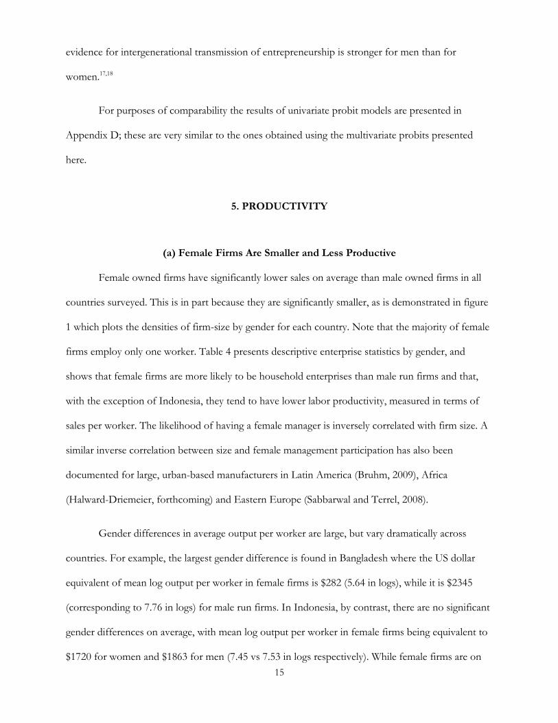
5. PRODUCTIVITY

(a) Female Firms Are Smaller and Less Productive

Female owned firms have significantly lower sales on average than male owned firms in all

countries surveyed. This is in part because they are significantly smaller, as is demonstrated in figure

1 which plots the densities of firm-size by gender for each country. Note that the majority of female

firms employ only one worker. Table 4 presents descriptive enterprise statistics by gender, and

shows that female firms are more likely to be household enterprises than male run firms and that,

with the exception of Indonesia, they tend to have lower labor productivity, measured in terms of

sales per worker. The likelihood of having a female manager is inversely correlated with firm size. A

similar inverse correlation between size and female management participation has also been

documented for large, urban-based manufacturers in Latin America (Bruhm, 2009), Africa

(Halward-Driemeier, forthcoming) and Eastern Europe (Sabbarwal and Terrel, 2008).

Gender differences in average output per worker are large, but vary dramatically across

countries. For example, the largest gender difference is found in Bangladesh where the US dollar

equivalent of mean log output per worker in female firms is $282 (5.64 in logs), while it is $2345

(corresponding to 7.76 in logs) for male run firms. In Indonesia, by contrast, there are no significant

gender differences on average, with mean log output per worker in female firms being equivalent to

$1720 for women and $1863 for men (7.45 vs 7.53 in logs respectively). While female firms are on

16

average less productive, labor productivity is highly dispersed, as is shown in figure 2 which plots the

densities of output per worker by gender for each country. This dispersion is indicative both of the

high heterogeneity of the non-farm sector, which comprises a wide variety of activities, and of

market power. Most firms face very few competitors, if any.

At first sight, differences in labor productivity do not appear driven by differences in capital

intensity. Surprisingly, male enterprises do not appear to use significantly more capital per worker

than female ones.19 These findings do not necessarily indicate an absence of gender differences in

access to capital; it is very well possible that women sort into certain sectors, which operate on a

relatively smaller scale. Since they are larger, male firms tend to use more capital in absolute terms.

Sector sorting patterns by gender are very pronounced, but vary from country to country.

For instance, in Bangladesh 95% of all female firms are engaged in manufacturing and almost none

are trading firms while 49% of all male firms are in trade and only 28% are in manufacturing. In

Ethiopia too, women are overrepresented relative to men in manufacturing, which accounts for the

bulk of non-farm enterprise activity. By contrast, in Indonesia, only 3% of all female firms are in

manufacturing compared with 14% of all male firms. In this case, women are overrepresented in the

trade sector. The fact that gender segregation patterns are less stark in Indonesia may help explain

why gender productivity differentials are not statistically significant in Indonesia. Note, however,

that these broad sector categories hide sorting into different subsectors (see appendix A for a

description of these different subsectors).

Differences in output per worker could also be due to differences in input usage and human

capital. With the exception of Indonesia, male firms use significantly more inputs per worker and

male entrepreneurs are better educated, on average, than their female counterparts.

17

(b) Empirical Strategy

To examine to what extent differences in output per worker are due to differences in factor

inputs and human capital, sorting into different sectors, returns to scale, we estimate Cobb-Douglas

production functions, modeling output of firm i in sector j, as a function of capital, ,

labor, , material inputs, , and Total Factor Productivity (TFP), which is in turn modeled as a

function of sector, S, firm characteristics F, characteristics of the manager, E, and a host of

investment climate characteristics, IC:

, where

. Taking-logs and adding these and an error term, v, our most general estimating

equation becomes:

(4)

where j subscripts denote sector specific factor coefficients, as we allow capital, labor and material

inputs coefficients to vary freely across sectors. In our empirical specification, we progressively add

explanatory variables to examine to what extent these different sets of explanatory variables account

for gender differences in output. Differences in productivity could also derive from differences in

returns to scale. If returns to scale are increasing (

, the larger size of male firms

may account for their higher average productivity. Alternatively, differences in productivity may

stem from sector selection. Note that these mechanisms may interact if returns to scale vary across

sectors. In appendix E we present specifications where we interact all variables used to explain total

factor productivity with a dummy for a having a female manager, to allow for gender differences in

the returns to human capital, experience and various investment climate proxies. The results suggest

that gender differences in the impact of these variables are generally statistically negligible.

This approach has well-known limitations. Measurement error in explanatory variables or

omitted variables may lead to biased estimates of productivity differentials. Despite having a rich and

18

detailed dataset, we cannot directly control for potentially important variables such as demand and

price differences. In principle, such endogeneity problems could be remedied by means of

instrumental variable estimation but, unfortunately, credible instruments are not available in our

data. However, using the same Ethiopian dataset as considered in this paper, but focusing only on

small manufacturing firms Loening et al. (2008) argue that endogeneity bias is likely to be small.

Using precipitation based indicators of local agricultural performance as a proxy for unobserved

local demand, they find that while better local agricultural performance is strongly correlated with

firm sales, their parameter estimates are not very sensitive to controlling for this variable, indicating

that endogeneity bias is small. Moreover, firms do not frequently adjust factor inputs, despite facing

frequent shocks, another reason why the impact of endogeneity bias may be limited.

Finally, this approach only focuses on the direct impact of gender and the investment

climate on firm productivity. However, perhaps the most important gender and investment climate

effects are indirect. For example, the investment climate may also impact on allocative efficiency (see,

e.g. Mengistae and Honorati, 2009), investment and growth, a possibility which is investigated in

Appendix F, which shows that, prima facie, gender differences in growth and investment

performance are small. It could also induce women to sort into small-scale low productivity sectors.

In short, we have to be cautious when interpreting the results from these models.

(c) Results

The regressions are estimated separately for each country. Results are presented in Table 5.

The dependent variable is the log of sales in US dollars. We present five different models. The first

model only includes a gender dummy while the second model adds a control for firm size.

Subsequent models add controls for sector (model 3), factor usage and differences in technology

across sectors (model 4) as well as other firm, human capital and investment climate characteristics

(model 5).20

19

Models 1 and 2 confirm that raw performance gaps are large in Bangladesh, Ethiopia and Sri

Lanka. These performance gaps are in part the result of sorting by size, (model 2), but appear to be

predominantly driven by sorting into different sectors (model 3) and material inputs usage (model 4);

once sector and factor usage are controlled for performance gaps reduce dramatically and the

explanatory power of our model shoots up, as is evidenced by the big increases in the R2s when we

add these explanatory variables. In Sri Lanka, the male-female productivity differential is entirely

explained by sorting. In Bangladesh, the gender differential reverses sign, while in Ethiopia the

productivity gap roughly halves. Parameter estimates appear reasonably well behaved, although it is

likely that the coefficients on capital are biased downwards due to measurement error. Capital- and

labor coefficients vary substantially across countries and sectors, reflecting cross-country differences

in the composition of the various sectors.

Adding controls for human capital, firm characteristics and the investment climate (model 5)

does not change results very much and increases explanatory power only slightly, suggesting that

most of the productivity differential is accounted for by sorting into different sectors and factor

usage. Gender productivity differences do not disappear altogether. The positive premium

associated with being a female manager in Bangladesh may not be well identified since there are

relatively few female firms in our Bangladeshi sample. Alternatively, it could be due to the fact that

female entrepreneurs are a highly eclectic group. The low productivity of female-run firms in

Ethiopia may in part be driven by sorting into different activities that our crude sector controls do

not capture. They may also reflect gender differences in hours worked, as we only observe

differences in labor days in Ethiopia. If women combine working in a non-farm firm with

household chores, they may work fewer hours in any given day.

The final specification furthermore suggest that household-based enterprises are on average

less productive than stand-alone firms, that older firms are more productive (although the

20

coefficient on firm age is statistically significant only in Indonesia and Sri Lanka), and that

investment climate variables are not very important determinants of firm performance. However, as

alluded to in section 5(b) their most important impact may be dynamic, a possibility which we

investigate in appendix F21. Moreover, it is remarkable how much the importance of different

factors, such as schooling, electricity usage, and location, varies across countries, underscoring how

heterogeneous the non-farm sector is across different countries.

The hypothesis of constant returns to scale is not rejected in the vast majority of cases. It is

rejected, however, at the 5% level for services and trading firms in Indonesia, and at the 10% level

for manufacturing firms in Bangladesh. In these cases, returns to scale are decreasing. If anything,

such decreasing returns to scale would minimize gender productivity differentials as male firms tend

to be larger (though not in Indonesia). By contrast, constant returns to scale are also rejected at the

10% level for Sri Lankan manufacturing firms, which seem to be characterized by mildly increasing

returns to scale. All in all, returns to scale do not appear an important determinant of gender

productivity differentials.

Overall, it seems that the evidence for gender differences in the returns to human capital is

limited. In addition, we find little evidence for gender asymmetries in the direct impact of the

investment climate on firm performance. Nor do we find evidence for gender differences in

productivity differentials associated with firm age and electrification. Moreover, differences in

returns to scale do not appear to explain gender productivity differentials; while male entrepreneurs

run larger firms we do not find evidence for increasing returns to scale. We do, however, find strong

evidence for differences in productivity due to sorting into different types of activities, factor usage

and firm size.

21

6. CONCLUSION

In spite of their increasing policy-prominence, relatively little is known about gender

inequities in rural non-agricultural labor market outcomes. This is unfortunate since non-farm

enterprises account for a substantial share of rural income and employment (Haggblade, Hazell and

Reardon, 2007). Using novel matched household-enterprise-community datasets from Bangladesh,

Ethiopia, Indonesia and Sri Lanka we attempt to redress this lacuna in the literature by documenting

and analyzing gender differences in individuals’ activity portfolio choices, as well as differences in

the productivity of rural non-farm firms.

Women are much less likely to engage in income earning activities and gender differences in

non-farm entrepreneurship are large. Women have lower participation rates in non-farm enterprise

activities in Bangladesh, Indonesia and Sri Lanka, but not in Ethiopia. However, working in rural

non-farm firms appears to be very important for women who partake in income earning activities

and especially so for those who are the heads of their households. Somewhat surprisingly, women’s

propensity to be non-farm entrepreneurs is not strongly correlated with their educational attainment

or the number of children in the household, whereas the share of children in the households is

negatively correlated with women’s engagement in wage employment in Bangladesh and Indonesia.

This suggests that running a non-farm firm is more compatible with combining domestic work with

income earning activities than wage employment is, which is consistent with most non-farm

enterprises managed by women being home-based. Women’s activity choices are also correlated

with their husbands’ educational attainment, with women whose partners have either very little, or a

lot of education seemingly less likely to run non-farm firms, although this pattern is not very

pronounced.

Female firms are much smaller and much less productive on average, yet gender differences

in productivity vary dramatically across countries. Mean differences in log output per worker and

22

firm size suggest that firms run by Bangladeshi men on average produce more than ten times as

much output per worker than female firms, and are on average three times as large. In Ethiopia,

firms led by women are on average as large as firms led by men, yet their productivity per worker is

only approximately a third of that of firms run by men. In Sri Lanka gender differences in size and

productivity are less dramatic, but large nonetheless. By contrast, in Indonesia, where gender

segregation patterns are least pronounced, there are no significant gender differences in output.

Nonetheless, mean log size differentials suggest that male firms are on average a third larger than

female firms.

Such differences in performance are overwhelmingly driven by sorting. Once differences in

size and sector are accounted for, gender productivity differentials diminish. Differences in inputs

usage also provide part of the explanation. Once these are conditioned on, gender productivity

differentials become insignificant in Sri Lanka and reverse sign in Bangladesh, with male firms being

significantly less productive. Women’s productivity disadvantage only remains statistically significant

in Ethiopia. These conditional gender differences in performance are robust to including additional

controls for salient investment climate characteristics.

Gender differences in productivity are not due to returns to scale; while male owned firms

are much larger, we did not find strong evidence of increasing returns to scale. In the few cases

where returns to scale were not constant, they tended to be decreasing, rather than increasing. Nor

are productivity differentials driven by differences in capital intensity: capital labor ratios do not

significantly vary by gender in any of the countries considered. Moreover, our regressions do not

support the hypothesis that differences in human capital account for gender differences in firm

performance, even though male managers are on average much better educated than female

managers. Similarly, we found little support for the idea that gender productivity differences are due

to a differential gender impact of the local investment climate.

23

Overall, our results demonstrate large gender disparities in rural off-farm labor market

outcomes. While we have managed to rule out a large number of candidate explanations for the

existence of these differences, fully understanding why these gender differences arise requires

additional research. Collecting panel data would help us better understand the causal mechanisms

underlying the patterns documented in this paper and would permit a richer representation of the

dynamics of rural labor markets.

24

7. REFERENCES

Altonji, J.and Blank. R. (1999). “Race and Gender in the Labor Market.”. In O. Ashenfelter and D.

Card (Eds.), Handbook of Labor Economics (Vol. 3, pp 3143-3259). Amsterdam, Netherlands: Elsevier

Science, B.V.

Attanasio, O. and Lechene, V. (2002). “Tests of Income Pooling in Household Decisions”. Review of

Economic Dynamics, Vol. 5 (4), 720-748.

Babatunde, R. O. and Qaim, M (2010). “Impact of off-farm income on food security and nutrition

in Nigeria”. Food Policy, Vol. 35(4), 303-311.

Bardasi, E. and Abay ,G. (2007). “Gender and Entrepreneurship in Ethiopia.” Background paper to

the Ethiopia Investment Climate Assessment. Washington, DC: The World Bank.

Bardasi, E. and Sabarwal, S. (2009). “Gender, Access to Finance, and Entrepreneurial Performance

in Africa.” World Bank Mimeo.

Blanchflower, D.G., Levine, P. and Zimmerman, D. (2003). “Discrimination in the small business

credit market.” Review of Economics and Statistics, Vol. 85 (4), 930-943.

Bruhm, M. (2009). “Female-Owned Firms in Latin America: Characteristics, Performance, and

Obstacles to Growth.” World Bank Policy Research Working Paper No. 5122

Brush, C. G. (1992). “Research on Women Business Owners: Past Trends, a New Perspective and

Future Directions.” Entrepreneurship: Theory and Practice 16.

Buvinić, M. and Gupta, G.R. (1997). “Female-Headed Households and Female-Maintained Families:

Are They Worth Targeting to Reduce Poverty in Developing Countries?” Economic Development and

Cultural Change, Vol. 45 (2), 259-280.

25

Carter, S. (2000). “Improving the numbers and performance of women-owned businesses: some

implications for training and advisory services.” Education + Training, Vol. 42 (4/5), 326 – 334.

Cavalluzzo, K.S. and Wolken, J. (2002). “Small Business Loan Turndowns, Personal Wealth and

Discrimination.” Finance and Economics Discussion Series 2002-35. Washington, D.C.: Board of Governors

of the Federal Reserve System.

Chen, S. And Ravallion, M., (2010). "The Developing World Is Poorer Than We Thought, but No

Less Successful in the Fight Against Poverty," The Quarterly Journal of Economics, Vol. 125 (4), 1577-

1625.

Davis, S. J., and Haltiwanger, J. (1992). “Gross Job Creation, Gross Job Destruction, and

Employment Reallocation.” Quarterly Journal of Economics, Vol. 107 (3), 819–63.

Davis, S. J., and Haltiwanger, J. (1999). “On the Driving Forces behind Cyclical Movements in

Employment and Job Reallocation.” American Economic Review Vol. 89 (5), 1234–58.

de Janvry, A. and Sadoulet, E. (2001). “Income Strategies Among Rural Households in Mexico: The

Role of Off-farm Activities.” World Development, Vol. 29 (3), 467-480.

Deininger, K., Jin, S. and Sur, M. (2007). "Sri Lanka's Rural Non-Farm Economy: Removing

Constraints to Pro-Poor Growth," World Development, Vol. 35 (12), 2056-2078.

Dercon, S. (2009). "Rural Poverty: Old Challenges in New Contexts," World Bank Research Observer,

Vol. 24 (1), 1-28.

Duflo, E. (2000). "Grandmothers and Granddaughters: Old Age Pension and Intra-household

Allocation in South Africa." NBER Working Papers 8061, National Bureau of Economic Research,

Inc

26

Easterly, W. (2002). “The Cartel of Good Intentions: Bureaucracy versus markets in foreign aid.‟

Center for Global Development Working Paper 4.

Goldstein, M. and Udry, C. (2008). “The profits of power: land rights and agricultural investment in

Ghana”. Journal of Political Economy, Vol. 116 (6), 981-1022.

Haddad, L. J., Hoddinott, J. and Alderman, H. (1997). Intra-Household Resource Allocation in Developing

Countries. Baltimore, MD: Johns Hopkins Univ. Press.

Haggblade, S., Hazell, P. and Reardon, T. (2007). Transforming the rural nonfarm economy. Baltimore,

MD: Johns Hopkins University Press and International Food Policy Research Institute.

Haggblade, S., Hazell, P. and Reardon, T. (2010). “The Rural Non-farm Economy: Prospects for

Growth and Poverty Reduction.” World Development, Vol. 38 (10), 1429–1441.

Hallward-Driemeier, M.. "Expanding Opportunities for Women Entrepreneurs in Africa." World

Bank (forthcoming).

Hallward-Driemeier, M. and Aterido R. (2009). “Whose Business Is It Anyway?” World Bank

Mimeo..

Headey, D., Bezemer, D. and Hazell, P. (2010). “Agricultural Employment Trends in Asia and

Africa: Too Fast or Too Slow?” World Bank Research Observer Vol. 25(1), 57-89.

Horrell, S. and Krishnan, P. (2007). “Poverty and Productivity in Female-Headed Households in

Zimbabwe.” Journal of Development Studies, Vol. 43 (8),1351-1380.

FAO, IFAD and ILO (2011). “Gender dimensions of agricultural and rural employment:

Differentiated pathways out of poverty”.

27

Jamison, D. and Lau, L.J. (1982). “Farmer education and farm efficiency” World Bank Research

Publication. Published for the World Bank by Johns Hopkins University Press.

Jin, S. and Deininger, K. (2009). "Key Constraints for Rural Non-Farm Activity in Tanzania:

Combining Investment Climate and Household Surveys." Journal of African Economies, Vol. 18(2), 319-

361.

Katz, E. and Chamorro, J. S. (2002). “Gender, land rights, and the household economy in rural

Nicaragua and Honduras.” Paper prepared for USAID/BASIS CRSP. Madison, Wisconsin.

Lanjouw, J. and Lanjouw, P. (2001). “The rural non-farm sector: Issues and evidence from

developing countries.” Agricultural Economics, Vol 26(1), 1–23.

Lanjouw, P. (2001). “Nonfarm Employment and Poverty in Rural El Salvador.” World Development

Vol. 29 (3), 529-547.

Loening, J. L., Rijkers, B. and Söderbom, M. (2008). “Non-farm microenterprises and the

investment climate: Evidence from rural Ethiopia.” World Bank Policy Research working paper

4577.

Lustig, N. (2000) “Crises and the Poor: Socially Responsible Macroeconomics.” Economía, Vol. 1 (1),

1-19.

Mammen, K. and Paxson, C. (2000). "Women's Work and Economic Development." Journal of

Economic Perspectives, Vol. 14(4), 141–164

McCulloch, Weisbrod, N. J. and Timmer, C. P. (2007). “The pathways out of rural poverty in

Indonesia.” World Bank Policy Research Working Paper 4173.

Mengistae, T. and Honorati, M. (2009). “Constraints to productivity growth and to job creation in

the private sector.” In Ethiopia investment climate assessment. Washington, DC: World Bank.

28

Parker, S. (2008). "Entrepreneurship among married couples in the United States: A simultaneous

probit approach," Labour Economics, Vol. 15 (3), 459-481.

Parker, S. (2009). The Economics of Entrepreneurship. Cambridge University Press

Priebe, J., Rudolf, R., Klasen S. and Weisbrod, J. (2009). “Rural income dynamics in post-crisis

Indonesia.” Paper presented at the Inaugural conference of courant research center – Poverty, equity

and growth in developing and transition countries. Göttingen, Germany.

Quisumbing, A.R. and. Maluccio, J.A. (2000). “Intrahousehold allocation and gender relations: New

empirical evidence from four developing countries.” IFPRI FCND Discussion Paper No. 84.

Rijkers, B., Soderbom, M. and Loening, J. (2010). “A Rural-Urban Comparison of Manufacturing

Enterprise Performance in Ethiopia.” World Development, Vol. 38 (9), 1278-1296.

Sabarwal, S. and Terrell, K. (2008). “Does Gender Matter for Firm Performance? Evidence from

Eastern Europe and Central Asia” World Bank Policy Research Working Paper no 4705.

Schady, N., and Rosero, J. (2007). “Do Cash Transfers to Women Affect the Composition of

Expenditures? Evidence on Food Engel Curves in Rural Ecuador.” World Bank Policy Research

Paper 4282.

Storey, D. J. (2004). “Racial and Gender Discrimination in the Micro Firms Credit Market?:

Evidence from Trinidad and Tobago.” Small Business Economics, Vol. 23(5), 401-422.

Thomas, D. (1990). “Intra-Household Resource Allocation: An Inferential Approach.” The Journal of

Human Resources, Vol. 25 (4), 635-664.

Udry, C. (1996) “Gender, Agricultural Production, and the Theory of the Household”. The Journal of

Political Economy , Vol. 104(5), 1010-1046.

29

World Bank (2004). “Investment Climate Assessment Sri Lanka: Improving the Rural and Urban

Investment Climate.”.

World Bank (2005). “A Better Investment Climate for Everyone” World Development Report 2005.

Washington DC: World Bank.

World Bank (2011). “Gender Equality and Development” World Development Report 2012,

Washignton DC: World Bank.

Zwede and Associates (2002). “Jobs, Gender and Small Enterprises in Africa: Preliminary Report,

Women Entrepreneurs in Ethiopia.” ILO Office, Addis Ababa in association with SEED,

International Labour Office, Geneva.

30

1 See e.g. Thomas, 1990, Haddad, Hoddinott and Alderman, 1997, Duflo, 2000, Quisumbing and Maluccio, 2000,

Attanasio and Lechene, 2002, Katz and Chamorro, 2002, Schady and Rosero, 2007.

2 The World Bank defines the investment climate as the set of location-specific factors shaping the opportunities and incentives for

firms to invest productively, create jobs and expand (World Bank, 2005, p19). De facto, any factor that affects firm performance

and decision making can be considered part of the investment climate. This has led some (e.g. Easterly, 2002) to criticize

the concept as being devoid of any meaning. Instead, we take the view that it is important to clearly specify which

aspects of the investment climate we are considering.

3 For example, in the Amhara region in Ethiopia, where the Ethiopian Rural Investment Climate Survey data used in this

paper were collected, the belief that the harvest will be bad if women work on the farm is prevalent (Zwede and

Associates, 2002, Bardasi and Getahun, 2007).

4 Gender differences in the performance of male and female entrepreneurs in developed countries are relatively well

documented, but the evidence is mixed. Some studies report evidence of female underperformance, whereas other do

not find gender differences (see e.g. the literature reviews in Parker, 2009 and Sabbarwal and Terrel, 2008).

5 In addition, Sabbarwal and Terrel (2008) find some evidence that female firms in Eastern Europe and Central Asia

have higher returns to scale, but the differences in returns to scale between men and women are small, and could be an

artifact of a rather restrictive production function specification. For example, differences in technology between sectors

are modeled as being additive in TFP, rather than as interacting with the returns to capital, labor and material inputs.

6 Some studies suggest women indeed have more difficulty accessing finance than men (e.g. Brush 1992, Carter, 2000),

while others detect no gender differences (Blanchflower et al., 2003, Storey, 2004, Cavalluzzo and Wolken, 2005).

7 Thus, in many cases the term “activity” might have been more appropriate than the term enterprise.

8 Loening et al (2008) demonstrate that the rural non-farm sector in the Amhara region is very similar to the rural non-

farm sector in other regions, although its composition is slightly skewed towards manufacturing activities, whereas in

other regions of Ethiopia trade and services enterprises dominate.

9 Only three enterprises in the Ethiopian dataset employ more than 10 workers. Since the enterprises in this dataset are

all household-based we might miss out on fully commercial enterprises owned or managed by individuals not living in

these communities. However, from the community level dataset one can infer that there are not more than a dozen

firms with more than 20 employees in a radius of one hour commuting distance from the 179 surveyed communities. It

31

thus seems safe to conclude that there are very few large firms in rural areas in Ethiopia, and that their absence from our

data is not an artifact of our sampling strategy.

10 The phrasing of the different questions about individual’s activity portfolios varied across countries, forcing us to

come up with an arbitrary categorization (see the appendix for details). In Indonesia, information on individuals’

engagement in agricultural activities was not available.

11 Of course, it is possible that individuals engage in different types of self-employment or hold multiple wage jobs in

which case they would misleadingly be classified as engaging in one activity only.

12 The participation rates documented in Table 1A may deviate somewhat from those reported in official statistics partly

because of sample coverage and partly because we are counting employment in home-based enterprises as labor market

participation.

13 Since subjective investment climate indicators may be endogenous to performance, we prefer objective proxies

instead.

14 Note, however, that the error terms for the NFE and agriculture participation probits are significantly negatively

correlated for the sample of Ethiopian women, suggesting they are substitutes in this context.

15 Female headed households are typically headed by widows.

16 Note that this effect is not present in Bangladesh, perhaps because female participation rates are low.

17 Individuals in households of which the head’s father held a wage job are significantly less likely to work in agriculture

and significantly more likely to hold a wage job. Individuals in households where the head’s father’s main source of

income was running a non-farm firm are ceteris paribus more likely to be engaged in NFE activity, but this effect is not

always statistically significant. In both Sri Lanka and Bangladesh, such individuals are also significantly less likely to

work on a family farm.

18 This difference may in part be due to the fact that we are using the household head father’s employment instead of

each individual’s father’s employment. Since men are more likely to be the head of their household, our measure may be

a better proxy for men than for women.

19 This conclusion is robust to using alternative measures of the capital stock, such as the replacement value of

machinery and equipment.

20 It would have been of interest to examine whether enterprises run by female household heads are more or less

productive than other female firms. However, our data do not enable us to cleanly identify whether the enterprise

manager is also the household head.

32

21 Analysis showed that gender differences in investment and growth rates are small and typically insignificant, a finding

which is robust to controlling for a rich set of firm, manager and investment climate characteristics.

33

Tables

Table 1A: Structure of the labor market – Bangladesh, Sri Lanka, Ethiopia

Participation Rates Bangladesh Ethiopia Indonesia Sri Lanka Women Men Women Men Women Men Women Men OLF/Not working (i) 68.24% 4.85% 25.69% 7.26% NA NA 50.74% 12.52% NFE only (ii) 5.46% 23.34% 5.56% 5.12% 8.78% 14.29% 19.09% 18.72% NFE + Agriculture (iii) 2.81% 19.24% 3.66% 4.18% NA NA 4.21% 12.00% NFE + Wage(iv) 0.21% 6.50% 0.31% 0.20% 1.10% 2.66% 1.17% 4.22% Agriculture only (v) 17.87% 14.51% 60.37% 70.30% NA NA 8.67% 11.01% Agriculture + Wage (vi) 0.86% 8.05% 1.73% 7.77% NA NA 1.36% 8.17% Wage only (vii) 4.37 % 19.79% 2.68% 5.17% 23.05% 44.53% 14.17% 31.38% Wage + Ag + NFE (viii) 0.12% 3.70% NA NA NA NA 0.39% 1.98%

Total NFE(sum ii, iii, iv, viii) 8.60% 52.78% 9.53% 9.50% 9.88% 16.35% 24.86% 36.92% Total Ag (sum iii, v, vi, viii) 21.66% 45.50% 65.76% 82.25% NA NA 14.63% 33.16%

Total wage sum(iv, vi, vii, viii) 5.56% 38.04% 4.72% 13.14% 24.45% 47.19% 17.09% 45.75%

Total multiple activities (sum iii, iv, vi, viii)

4.00% 37.49% 5.70% 12.15% NA NA 7.13% 26.37%

Conditional on Working

NFE only (ii) 17.19% 24.53% 7.48% 5.52% 38.76% 21.25% NFE + Agriculture (iii) 8.85% 20.23% 4.93% 4.51% 8.54% 13.72%

NFE + Wage(iv) 0.67% 6.83% 0.42% 0.22% 2.37% 4.82%

Agriculture only (v) 56.26% 15.25% 81.24% 75.80% 17.61% 12.58% Agriculture+ Wage (vi) 2.70% 8.46% 2.32% 8.38% 2.76% 9.34%

Wage only (vii) 13.77% 20.80% 3.61% 5.57% 28.78% 35.87%

Wage + Ag + NFE (viii) 0.38% 3.89% 0.79% 2.26%

Total NFE(sum ii, iii, iv, viii) 27.09% 55.48% 12.83% 10.25% 50.46% 42.05% Total Ag (sum iii, v, vi, viii) 68.19% 47.83% 88.49% 88.69% 29.70% 37.90%

Total wage sum(iv, vi, vii, viii) 17.52% 39.98% 6.35% 14.17% 34.70% 52.29% Total multiple activities (sum iii, iv, vi, viii)

12.60% 39.41% 7.67% 13.11% 14.46% 30.14%

Note: statistics are weighted in Bangladesh, Ethiopia and Indonesia, but not in Sri Lanka since household weights were not available for that country. Ag=working on the family farm, Wage=wage employment (a composite category covering both agricultural and non-agricultural wage employment) NFE=non-farm enterprise activity; working in a household non-farm enterprise. The categories presented in this table were constructed on the basis of different questions (see the appendix for specifics).

34

Table 1B: Household-level participation Rates in NFE

Household- level Participation Rates

Overall Male-headed Female-headed

% of hh that are female-headed

Bangladesh 27.62% 28.61% 16.79% 8.32% Ethiopia 16.20% 12.13% 31.08% 21.46% Indonesia 23.32% 24.69% 15.23% 14.45% Sri Lanka 47.15% 48.80% 37.95% 14.78%

% of households that work exclusively in own non-farm enterprises

Overall Male-headed Female-headed

Bangladesh 13.66% 13.93% 10.07% Ethiopia 4.86% 2.12% 15.83% Sri Lanka 13.72% 13.80% 13.25%

% of households whose only source of pecuniary income is non-farm enterprise income

Overall Male-headed Female-headed

Ethiopia 4.47% 2.11% 13.11% Indonesia 2.70% 2.82% 1.99%

Note: statistics are weighted in Bangladesh, Ethiopia and Indonesia, but not in Sri Lanka since household weights were not available for that country.

35

Table 2: Individual Characteristics

Descriptive Statistics Individuals Bolded numbers indicate gender differences are statistically significant at the 5% level.

Bangladesh Ethiopia Indonesia Sri Lanka

Women Men Women Men Women Men Women Men

mean se mean se mean se mean se mean se mean se mean se mean se

NFE 0.09 0.28 0.53 0.50 0.09

.292874

6

0.09

.29287

46

0.10 0.30 0.10 0.30 0.17 0.37 0.26 0.44 0.37 0.48 agriculture 0.22 0.42 0.47 0.50 0.67 0.67

.46858

38

0.85 0.35

0.15 0.36 0.34 0.47

wage 0.06 0.23 0.38 0.49 0.05 0.21 0.15 0.36 0.24 0.43 0.47 0.50 0.18 0.38 0.45 0.50

age 35.04 12.70 34.78 12.64 33.16 12.30 34.50 12.69 35.64 13.15 35.05 12.73 36.94 12.29 37.10 12.78

primary 0.30 0.46 0.37 0.48 0.06 0.24 0.24 0.42 0.40 0.49 0.43 0.50 0.19 0.39 0.18 0.39

secondary 0.31 0.46 0.34 0.47 0.02 0.13 0.03 0.17 0.34 0.47 0.38 0.48 0.75 0.43 0.78 0.42

tertiary 0.01 0.10 0.05 0.22

0.04 0.21 0.07 0.25 0.02 0.13 0.02 0.13

head 0.05 0.22 0.56 0.50 0.17 0.38 0.72 0.45 0.08 0.28 0.55 0.50 0.08 0.27 0.56 0.50

spouse 0.61 0.49 0.01 0.08 0.67 0.47 0.01 0.09 0.60 0.49 0.00 0.04 0.56 0.50 0.02 0.13

child 0.26 0.44 0.39 0.49 0.12 0.33 0.20 0.40 0.26 0.44 0.39 0.49 0.31 0.46 0.40 0.49

married 0.79 0.40 0.72 0.45 0.71 0.45 0.74 0.44 0.72 0.45 0.64 0.48

widow/divorced 0.12 0.32 0.00 0.07 0.21 0.40 0.05 0.22 0.11 0.31 0.05 0.22

ln hh size 1.61 0.42 1.65 0.38 1.50 0.50 1.56 0.44 1.45 0.44 1.49 0.44 1.51 0.37 1.52 0.35

sh child 0.19 0.18 0.18 0.18 0.28 0.20 0.29 0.20 0.16 0.17 0.16 0.17 0.13 0.17 0.12 0.17

sh elderly 0.04 0.10 0.03 0.08 0.03 0.08 0.02 0.06 0.05 0.12 0.04 0.10 0.04 0.10 0.04 0.10

electricity 0.88 0.33 0.90 0.30 0.04 0.20 0.03 0.17 0.96 0.20 0.96 0.19 0.96 0.20 0.95 0.21

town 0.11 0.31 0.13 0.33 0.05 0.22 0.04 0.19 0.32 0.47 0.30 0.46

ln dist market 0.80 0.57 0.81 0.57 2.05 0.81 2.10 0.77 1.14 1.02 1.10 1.03 1.93 0.90 1.96 0.90

credit inst 0.24 0.43 0.23 0.42 0.33 0.47 0.33 0.47 0.19 0.39 0.19 0.39 0.52 0.50 0.50 0.50

ln local wage 6.00 0.25 6.02 0.25 5.56 0.41 5.57 0.41 6.23 0.48 6.22 0.49 6.69 0.24 6.69 0.24

partner primary 0.22 0.41 0.20 0.40 0.17 0.37 0.04 0.20 0.27 0.45 0.26 0.44 0.15 0.35 0.13 0.33

partner secondary 0.17 0.38 0.12 0.33 0.01 0.12 0.01 0.07 0.16 0.37 0.13 0.34 0.41 0.49 0.40 0.49

partner tertiary 0.02 0.13 0.01 0.09

0.04 0.19 0.02 0.15 0.01 0.10 0.01 0.09

h father Ag 0.65 0.48 0.63 0.48

0.56 0.50 0.56 0.50 0.44 0.50 0.44 0.50

h father NFE 0.17 0.37 0.18 0.39

0.10 0.30 0.10 0.30 0.26 0.44 0.25 0.43

h father wage 0.18 0.39 0.18 0.39

0.31 0.46 0.32 0.47 0.26 0.44 0.27 0.44

h father other 0.10 0.30 0.17 0.37 0.02 0.15 0.03 0.16

Note: Statistics are weighted except for Sri Lanka.

36

Table 3A: Bangladesh and Ethiopia

Participation in Bangladesh and Ethiopia (1/2) Table continues on the next page

Bangladesh Trivariate probit models

Ethiopia

Trivariate probit models for women, univariate probit models for men

NFE Agriculture Wage

NFE Agriculture Wage

women men women men women men women men women men women men

coef/se coef/se coef/se coef/se coef/se coef/se coef/se coef/se coef/se coef/se coef/se coef/se

age 0.081** -0.012 0.114*** 0.012 0.041 -0.030

0.088*** 0.032 -0.021 -0.036 0.111*** 0.052**

(0.040) (0.044) (0.042) (0.039) (0.039) (0.038)

(0.023) (0.030) (0.018) (0.027) (0.025) (0.023)

age2/100 -0.136** 0.019 -0.147*** -0.008 -0.066 0.010

-0.111*** -0.049 0.009 0.041 -0.163*** -0.060**

(0.054) (0.052) (0.051) (0.047) (0.049) (0.045)

(0.028) (0.036) (0.023) (0.033) (0.033) (0.029) primary 0.110 0.261 0.399** -0.063 0.162 0.143

-0.161 0.241** 0.265** 0.011 -0.149 0.058

(0.169) (0.193) (0.195) (0.194) (0.258) (0.186)

(0.170) (0.096) (0.127) (0.105) (0.173) (0.088)

secondary 0.027 0.449** 0.200 -0.123 -0.173 -0.305**

-0.554** 0.283 -0.983*** -0.798*** 1.159*** 0.335*

(0.199) (0.181) (0.243) (0.185) (0.300) (0.148)

(0.275) (0.221) (0.323) (0.186) (0.282) (0.171)

tertiary -0.209 0.374 -2.540*** -1.025*** 1.727*** 0.731**

(0.571) (0.355) (0.485) (0.342) (0.450) (0.325)

head 1.068*** 0.278 0.437 0.047 0.387 -0.173

0.464** 1.045*** 0.308 1.579*** 0.027 -

1.291*** (0.343) (0.251) (0.332) (0.264) (0.462) (0.259)

(0.225) (0.270) (0.191) (0.203) (0.238) (0.210)

spouse 0.309 -0.407 0.297 -1.435*** -0.332 -0.127

-0.277 -0.417 0.288* 1.106** -0.970*** -

1.671*** (0.325) (0.461) (0.288) (0.481) (0.443) (0.436)

(0.239) (0.500) (0.175) (0.440) (0.222) (0.393)

child 0.232 0.029 -0.074 -0.475* 0.235 -0.295

-0.155 0.042 0.000 1.641*** -0.138 -

1.516*** (0.323) (0.201) (0.392) (0.258) (0.439) (0.223)

(0.209) (0.236) (0.181) (0.159) (0.223) (0.161)

married -0.558** 0.106 -1.062*** 0.480** -0.574* 0.136

-0.298 -0.037 0.230 0.425** 0.168 -0.139

(0.275) (0.195) (0.305) (0.212) (0.314) (0.179)

(0.217) (0.206) (0.161) (0.191) (0.201) (0.157)

widow/divorced 0.077 -1.398*** -0.242 -1.653** 0.187 0.689

0.072 0.015 0.427*** 0.089 0.019 -0.121

(0.416) (0.531) (0.396) (0.747) (0.523) (0.750)

(0.192) (0.224) (0.155) (0.198) (0.171) (0.199)

ln hh size -0.125 -0.078 -0.203 0.343* -0.237 -0.237

-0.305*** 0.406*** 0.266*** 0.105 -0.139 -0.265**

(0.203) (0.187) (0.218) (0.190) (0.245) (0.181)

(0.094) (0.130) (0.098) (0.127) (0.126) (0.116)

sh child 0.280 0.073 -0.166 0.046 -1.561** -0.168

0.363 -0.593** -0.589*** 0.268 0.113 0.428*

(0.411) (0.423) (0.546) (0.429) (0.657) (0.387)

(0.250) (0.277) (0.216) (0.278) (0.293) (0.245)

sh elderly 0.553 0.270 0.772 1.570 -0.919 -0.656

0.438 0.577 -0.502 1.923*** -0.214 -0.875

(0.856) (0.708) (0.779) (1.154) (0.978) (0.715)

(0.548) (0.806) (0.384) (0.713) (0.641) (0.649)

electricity -0.081 0.180 0.461* -0.173 0.494 -0.197

0.151 -0.234 -0.565*** -0.614*** 0.139 -0.049

(0.219) (0.194) (0.245) (0.227) (0.395) (0.176)

(0.131) (0.153) (0.187) (0.186) (0.230) (0.151)

town 0.477*** 0.822*** 0.340 -0.283* -0.183 -0.826***

0.677*** 0.857*** -1.815*** -1.071*** 0.085 0.541***

(0.164) (0.136) (0.238) (0.153) (0.239) (0.163)

(0.166) (0.183) (0.171) (0.187) (0.215) (0.166)

37

Participation in Bangladesh and Ethiopia (2/2) Table continued from the previous page

Bangladesh Trivariate probit models

Ethiopia

Trivariate probit models for women, univariate proibt models for men

NFE Agriculture Wage NFE Agriculture Wage

women men women men women men

women men women men women men

coef/se coef/se coef/se coef/se coef/se coef/se

coef/se coef/se coef/se coef/se coef/se coef/se

ln dist market 0.017 -0.074 0.061 -0.077 -0.051 -0.112

-0.358*** -0.315*** 0.077 0.364*** 0.014 -0.010

(0.119) (0.098) (0.123) (0.111) (0.237) (0.095)

(0.073) (0.075) (0.053) (0.069) (0.068) (0.050)

credit institution 0.056 0.392*** 0.056 -0.028 -0.246 -0.268**

0.084 -0.098 0.047 0.014 0.123 -0.034

(0.176) (0.149) (0.212) (0.147) (0.279) (0.128)

(0.095) (0.098) (0.068) (0.097) (0.101) (0.077)

ln local wage -0.452* -0.421 -0.856*** -1.102*** -0.656 0.216

-0.169* -0.083 -0.178* 0.058 -0.084 0.121

(0.265) (0.259) (0.330) (0.266) (0.459) (0.238)

(0.100) (0.107) (0.091) (0.102) (0.097) (0.093)

partner primary 0.034 -0.221 -0.147 0.084 0.565 -0.116

0.387*** -0.011 0.008 0.017 0.129 0.043

(0.180) (0.217) (0.207) (0.186) (0.386) (0.216)

(0.128) (0.170) (0.089) (0.178) (0.158) (0.154)

partner secondary -0.009 -0.313 0.139 0.070 0.696* 0.145

0.274 -0.454 -0.181 0.076 0.190 0.684**

(0.246) (0.199) (0.260) (0.190) (0.402) (0.194)

(0.358) (0.401) (0.246) (0.319) (0.285) (0.338)

partner tertiary 0.119 -1.408** -0.834 0.378 0.836* 0.574

(0.432) (0.693) (0.522) (0.615) (0.498) (0.569)

h father NFE 0.261* 0.193 -0.364* -0.489*** 0.101 0.150

(0.150) (0.179) (0.216) (0.170) (0.242) (0.153)

h father wage -0.071 -0.159 -0.592** -0.841*** 0.949*** 0.963***

(0.169) (0.154) (0.231) (0.179) (0.257) (0.160)

constant 2.326 3.984 6.487* 10.703*** 4.747 -0.860

-0.536 -1.863* 1.636** -1.283 -2.289*** -1.372*

(2.666) (2.665) (3.321) (2.850) (4.810) (2.557)

(0.905) (0.991) (0.823) (0.936) (0.844) (0.804)

ρ NFE-Ag 0.118 -0.047

-0.264***

(0.101) (0.082)

(0.061)

ρ NFE-Wage -0.221* -0.728***

-0.338***

(0.123) (0.109)

(0.109)

ρ Ag-Wage -0.249 -0.344***

-0.284***

(0.153) (0.093)

(0.064)

Observations 3,515 4,158

2,805 2,252

2,252

2,252

Pseudo R2

0.122

0.258

0.098

Log pseudolikelihood -2605305 -4901829

-2633

Wald chi2 58.36(23) 98.79(23)

393.87(19)

Note: *** p<0.01, ** p<0.05, * p<0.1. Regressions are weighted. Standard errors are heteroscedasticity robust and clustered at the household level.

38

Table 3B: Indonesia and Sri Lanka

Participation in Indonesia and Sri Lanka

Indonesia

Bivariate probit models Sri Lanka

Trivariate probit models

NFE Wage NFE Agriculture Wage women men women men women men women men women men coef/se coef/se coef/se coef/se coef/se coef/se coef/se coef/se coef/se coef/se age 0.121*** 0.011 0.093** 0.115*** 0.064*** 0.033 0.099*** 0.044 0.092*** 0.125***

(0.031) (0.035) (0.041) (0.032) (0.024) (0.022) (0.028) (0.027) (0.027) (0.022) age2/100 -0.142*** -0.014 -0.133** -0.165*** -0.086*** -0.033 -0.114*** -0.026 -0.136*** -0.177***

(0.038) (0.039) (0.054) (0.040) (0.029) (0.026) (0.035) (0.031) (0.036) (0.027) primary -0.319* -0.314* 0.005 0.019 0.285 0.153 0.354 0.185 0.070 0.363

(0.170) (0.184) (0.200) (0.187) (0.201) (0.289) (0.240) (0.272) (0.219) (0.257) secondary -0.064 -0.211 0.027 -0.123 0.158 0.638** 0.245 0.018 0.066 0.278

(0.174) (0.193) (0.227) (0.218) (0.194) (0.280) (0.234) (0.264) (0.212) (0.246) tertiary 0.115 -0.245 1.093*** 0.241 -0.165 -0.153 0.114 -0.562 1.087*** 1.127***

(0.269) (0.247) (0.269) (0.241) (0.377) (0.422) (0.524) (0.431) (0.362) (0.394) head 1.212*** 0.554** -0.176 0.899** 0.737*** 0.364 1.235*** 0.485 -0.166 0.390

(0.316) (0.260) (0.299) (0.353) (0.244) (0.286) (0.372) (0.363) (0.244) (0.280) spouse -0.163 -0.168 0.622* 0.753 0.526* -1.168** 0.662* -0.875* -0.101 1.457***

(0.294) (0.513) (0.338) (0.687) (0.293) (0.472) (0.399) (0.512) (0.314) (0.438) child -0.046 0.146 -0.218 0.714** 0.122 -0.082 0.512 0.120 0.073 0.420

(0.237) (0.272) (0.302) (0.293) (0.238) (0.252) (0.374) (0.331) (0.270) (0.265) married 0.334 0.666** 0.149 -0.087 0.062 0.174 -0.026 -0.430*** -0.130 -0.042

(0.216) (0.315) (0.226) (0.230) (0.130) (0.130) (0.130) (0.131) (0.129) (0.117) widow/divorced -0.086 -0.027 0.722** 0.262 -0.514* 0.131 0.556** 0.329 -0.746** -0.015

(0.299) (0.378) (0.338) (0.345) (0.272) (0.271) (0.281) (0.282) (0.297) (0.255) ln hh size 0.219* 0.048 -0.148 -0.130 -0.787 -0.396 1.025** 0.356 -0.339 0.275

(0.122) (0.140) (0.154) (0.176) (0.485) (0.424) (0.495) (0.446) (0.454) (0.423) sh child -0.432 -0.146 -0.788** 0.520 -0.188 0.216 0.071 0.059 -0.343 0.149

(0.300) (0.392) (0.392) (0.404) (0.224) (0.197) (0.251) (0.214) (0.271) (0.199) sh elderly -0.802* -0.622 0.507 0.927 -0.037 0.303* 0.119 0.101 -0.276 -0.207

(0.474) (0.594) (0.590) (0.571) (0.215) (0.182) (0.239) (0.203) (0.264) (0.185) electricity 0.286 0.684*** -0.460 -0.010 0.281 0.340* -0.557*** -0.574*** 0.135 0.263

(0.209) (0.247) (0.301) (0.273) (0.235) (0.198) (0.214) (0.200) (0.213) (0.200) town 0.245** 0.214* 0.261** 0.149

(0.117) (0.116) (0.124) (0.128) ln dist market -0.125** 0.024 -0.122** -0.244*** -0.054 0.030 -0.097* 0.194*** 0.082* -0.122***

(0.053) (0.047) (0.059) (0.062) (0.050) (0.050) (0.056) (0.049) (0.048) (0.046) credit institution 0.082 0.269** 0.251** -0.103 0.186** 0.278*** -0.293*** -0.229*** 0.060 -0.019

(0.109) (0.123) (0.127) (0.134) (0.085) (0.082) (0.094) (0.086) (0.087) (0.077) ln local wage -0.025 -0.074 -0.265** 0.019 0.282 0.314* -0.007 -0.229 -0.118 -0.279*

(0.125) (0.138) (0.131) (0.163) (0.187) (0.178) (0.207) (0.181) (0.201) (0.164) partner primary 0.425** -0.019 -0.386 0.109 -0.649 0.523 -0.300 0.251 0.331 -0.349

(0.203) (0.168) (0.243) (0.206) (0.477) (0.480) (0.678) (0.445) (0.499) (0.408) partner secondary 0.406** -0.093 -0.639** -0.060 0.064*** 0.033 0.099*** 0.044 0.092*** 0.125***

(0.203) (0.199) (0.259) (0.217) (0.024) (0.022) (0.028) (0.027) (0.027) (0.022) partner tertiary 0.362 0.002 -0.498 0.189 -0.086*** -0.033 -0.114*** -0.026 -0.136*** -0.177***

(0.271) (0.275) (0.323) (0.302) (0.029) (0.026) (0.035) (0.031) (0.036) (0.027) h father NFE 0.275** 0.475*** -0.259 -0.169 0.120 0.286*** -0.579*** -0.619*** 0.035 0.005

(0.128) (0.152) (0.175) (0.158) (0.104) (0.103) (0.135) (0.106) (0.110) (0.097) h father wage -0.151 -0.199 0.618*** 0.536*** 0.009 -0.011 -0.413*** -0.615*** 0.404*** 0.337***

(0.157) (0.138) (0.143) (0.156) (0.107) (0.100) (0.111) (0.104) (0.103) (0.093) h father other 0.004 -0.413 -0.479 -0.299 0.113 0.246

(0.299) (0.285) (0.341) (0.335) (0.245) (0.234) constant -4.091** -1.643 2.061 -2.624 -5.747*** -6.277*** -2.899 1.672 -1.005 0.408 (1.925) (2.188) (2.131) (2.675) (2.138) (2.033) (2.415) (2.092) (2.264) (1.886) ρ NFE-Ag

0.104* 0.066

(0.063) (0.054) ρ NFE-Wage -0.418*** -0.709***

-0.449*** -0.936***

(0.077) (0.091) (0.070) (0.072)

ρ Ag-Wage

-0.092 -0.308***

(0.071) (0.055) Observations 3,629 3,606

1359 1350 Log pseudolikelihood

-1068116 -1454910

-1804 -2176

Wald chi2 99.98(23) 170.13(23)

71.75(21) 187.28(21)

Note: *** p<0.01, ** p<0.05, * p<0.1. Regressions are weighted for Indonesia, but not for Sri Lanka since household weights were not

available. Standard errors are heteroscedasticity robust and clustered at the household level.

39

Table 4: Descriptive Statistics – Enterprises

Descriptive Statistics Enterprises Bolded numbers indicate gender differences are statistically significant at the 5% level.

Bangladesh Ethiopia Indonesia Sri Lanka

Women

Men

Women Men Women

Men

Women

Men

Variable mean se mean se mean se mean se mean se mean se mean se mean se

ln Y 5.42 1.26 8.16 1.48 4.52 1.78 5.45 1.83 7.74 1.48 8.10 1.66 6.35 1.54 7.27 1.61

ln L -0.22 0.53 0.40 0.70 -0.42 0.74 -0.55 0.92 0.29 0.88 0.57 1.05 0.35 0.49 0.57 0.60

hired L 0.08 0.28 0.31 0.46 0.02 0.14 0.06 0.24 0.25 0.44 0.44 0.50 0.34 0.47 0.52 0.50

share paid L 0.05 0.15 0.18 0.30 0.01 0.12 0.03 0.15 0.23 0.40 0.38 0.46 0.19 0.27 0.30 0.31

1 worker 0.76 0.43 0.32 0.47 0.80 0.40 0.73 0.44 0.60 0.49 0.44 0.50 0.57 0.50 0.38 0.48

2 workers 0.14 0.35 0.38 0.48 0.17 0.37 0.22 0.41 0.22 0.41 0.24 0.43 0.31 0.46 0.39 0.49

3-5 workers 0.10 0.29 0.23 0.42 0.03 0.16 0.04 0.21 0.15 0.36 0.18 0.39 0.09 0.28 0.19 0.39

5-50 workers 0.00 0.07 0.06 0.24 0.00 0.06 0.00 0.06 0.03 0.18 0.13 0.33 0.03 0.17 0.05 0.21

>50 workers 0.00 0.00 0.00 0.07 0.00 0.00 0.01 0.08 0.00 0.01 0.00 0.06 0.00 0.00 0.00 0.05

ln K 4.98 1.35 5.32 1.74 4.58 2.68 4.14 2.68 6.64 2.55 6.91 2.79 6.72 1.69 7.25 1.71

ln (Y/L) 5.64 1.15 7.76 1.35 4.95 1.62 6.00 1.90 7.45 1.40 7.53 1.41 6.02 1.46 6.71 1.45

ln (K/L) 5.21 1.40 4.92 1.60 4.92 2.53 4.50 2.65 6.34 2.58 6.34 2.87 6.37 1.67 6.68 1.61

ln (M/L) 3.94 1.68 7.22 1.74 3.79 2.15 4.85 2.62 6.72 1.54 6.51 1.68 5.35 1.57 6.28 1.56

invest 0.20 0.40 0.29 0.46 0.16 0.37 0.21 0.41 0.48 0.50 0.47 0.50 0.60 0.49 0.50 0.50

∆ ln L 0.01 0.07 0.03 0.22 0.06 0.72 0.11 0.53 0.08 0.29 0.10 0.40 0.01 0.09 0.00 0.11

L decreased 0.00 0.03 0.01 0.07 0.03 0.16 0.02 0.15 0.01 0.10 0.02 0.15 0.00 0.06 0.02 0.13

L increased 0.01 0.10 0.06 0.24 0.08 0.26 0.10 0.31 0.50 0.50 0.55 0.50 0.21 0.41 0.14 0.34

manufacturing 0.95 0.22 0.28 0.45 0.75 0.43 0.46 0.50 0.03 0.16 0.14 0.34 0.50 0.50 0.38 0.49

services 0.05 0.21 0.24 0.42 0.10 0.30 0.12 0.33 0.24 0.43 0.40 0.49 0.15 0.36 0.23 0.42

trade 0.00 0.05 0.49 0.50 0.14 0.35 0.41 0.49 0.73 0.44 0.47 0.50 0.34 0.48 0.39 0.49

hh enterprise 0.96 0.21 0.21 0.40 0.75 0.44 0.74 0.44 0.60 0.49 0.34 0.48

electricity usage 0.64 0.48 0.75 0.43 0.05 0.22 0.04 0.19 0.70 0.46 0.64 0.48 0.77 0.42 0.73 0.44

firm age 6.41 7.19 10.06 10.49 8.78 8.43 8.73 9.87 9.12 9.46 8.98 8.68 8.75 10.93 9.10 10.57

mngr age 31.64 8.53 39.25 13.45 43.18 13.04 41.67 13.73 40.00 12.10 41.40 11.34

mngr years experience

3.25 5.32 5.60 7.52

mngr primary 0.24 0.43 0.36 0.48 0.11 0.32 0.42 0.49 0.35 0.48 0.32 0.03 0.20 0.40 0.11 0.32

mngr secondary 0.36 0.48 0.42 0.49 0.03 0.17 0.05 0.23 0.42 0.49 0.42 0.03 0.77 0.42 0.86 0.35

mngr tertiary 0.00 0.05 0.04 0.20 0.09 0.29 0.17 0.03 0.02 0.14 0.03 0.16

town 0.50 0.50 0.46 0.50 0.29 0.45 0.21 0.41 0.51 0.50 0.51 0.50

ln dist market 0.61 0.40 0.67 0.50 1.16 1.00 1.64 0.93 0.66 0.97 0.93 1.12 1.51 0.92 1.81 1.14

credit institution 0.13 0.34 0.42 0.49 0.51 0.50 0.60 0.49 0.48 0.50 0.44 0.50 0.60 0.49 0.70 0.46

ln local wage 6.15 0.21 6.07 0.24 5.52 0.40 5.55 0.40 6.50 0.45 6.46 0.43 6.69 0.23 6.70 0.22

Note: Statistics are weighted. The samples are confined to observations for whom the production function could be estimated.

40

Table 5: Production Functions

Production Functions (1/2) Table continues on the next page

Bangladesh Ethiopia Indonesia Sri Lanka

coef se coef se coef se coef se

MODEL 1: GENDER ONLY mngr is male 2.744*** (0.206)

0.929*** (0.232) 0.143 (0.197) 0.917*** (0.178) Observations 2,480

648

1,369

1,259

R2 0.228

0.060

0.002

0.056

Adjusted R2 0.228

0.059

0.001

0.055

MODEL 2: GENDER AND SIZE

mngr is male 2.196*** (0.194) 0.998*** (0.226) -0.104 (0.187) 0.641*** (0.169) ln L 0.875*** (0.094) 0.561*** (0.128) 0.833*** (0.081) 1.200*** (0.091)

Observations 2,480

647

1,369

1,259

R2 0.359

0.125

0.256

0.223

Adjusted R2 0.359

0.123

0.255

0.221

MODEL 3: GENDER, SIZE AND SECTOR

mngr is male 0.998*** (0.290) 0.632*** (0.206) -0.067 (0.277) 0.514*** (0.157) ln L 1.252*** (0.105) 0.786*** (0.125) 0.790*** (0.088) 1.308*** (0.089)

services 0.463* (0.258) 0.092 (0.364) -0.439* (0.222) 0.619*** (0.196)

Trade 1.809*** (0.237) 1.443*** (0.261) -0.012 (0.367) 1.020*** (0.132)

Observations 2,480

647

1,369

1,259

R2 0.555

0.227

0.273

0.298

Adjusted R2 0.554

0.222

0.271

0.296

MODEL 4: GENDER, SIZE AND SECTOR (+ lnK and lnM) mngr is male -0.310** (0.124) 0.459*** (0.152) 0.076 (0.092) -0.010 (0.099) manuf*lnK 0.074*** (0.027) 0.073* (0.042) 0.027 (0.017) -0.005 (0.052)

manuf*lnL 0.229*** (0.042) 0.591*** (0.166) 0.344*** (0.121) 0.348*** (0.090)

manuf*lnM 0.668*** (0.029) 0.384*** (0.075) 0.599*** (0.087) 0.746*** (0.054)

serv*lnK 0.082*** (0.013) 0.167** (0.069) 0.048*** (0.017) 0.106** (0.042)

serv*lnL 0.423*** (0.047) 0.642*** (0.237) 0.256*** (0.075) 0.272 (0.167)

serv*lnM 0.536*** (0.022) 0.261*** (0.071) 0.563*** (0.046) 0.640*** (0.056)

trade*lnK 0.012 (0.009) 0.062 (0.038) 0.014 (0.013) 0.043* (0.024)

trade*lnL 0.182*** (0.038) 0.559*** (0.116) 0.142*** (0.046) 0.235* (0.122)

trade*lnM 0.847*** (0.023) 0.558*** (0.106) 0.752*** (0.051) 0.863*** (0.034)

services 0.839*** (0.281) 0.511 (0.533) 0.222 (0.793) 0.116 (0.532) Trade -1.097*** (0.301) -0.715 (0.710) -1.041 (0.770) -1.256** (0.529)

hh enterprise -0.320*** (0.047)

-0.525*** (0.160) -0.143* (0.080)

F TESTS – CRS

CRS-Manufacturing F(1, 169) = 1.44 F(1, 118) = 0.10 F(1, 160) = 0.06 F(1, 143) = 1.76

p>F 0.2321

0.7564

0.8018

0.1868

CRS-Services F(1, 169) = 0.84 F(1, 118) = 0.07 F(1, 160) = 5.24 F(1, 143) = 0.02 p>F 0.3598

0.7991

0.0234

0.8967

CRS-Trade F(1, 169) = 1.55 F(1, 118) = 1.48 F(1, 160) = 4.67 F(1, 143) = 1.81

p>F 0.2149

0.2266

0.0322

0.1812

Observations 2,480

537

1,369

1,058

R2 0.957

0.487

0.789

0.806

Adjusted R2 0.957

0.475

0.787

0.804

Note: *** p<0.01, ** p<0.05, * p<0.1. Regressions are weighted. Standard errors are heteroscedasticity robust and clustered at the village level.

41

Table 5: Production Functions

Production Functions (2/2) Table continued from the previous page

Bangladesh Ethiopia Indonesia Sri Lanka

coef se coef se coef se coef se

MODEL 5: ALL CONTROLS

mngr is male -0.242** (0.109) 0.606*** (0.161) 0.058 (0.072) -0.064 (0.111) manuf*lnK 0.073*** (0.026) 0.064* (0.034) 0.012 (0.019) -0.019 (0.052) manuf*lnL 0.224*** (0.042) 0.413*** (0.121) 0.367*** (0.116) 0.398*** (0.094)

manuf*lnM 0.654*** (0.029) 0.467*** (0.073) 0.552*** (0.091) 0.733*** (0.056)

serv*lnK 0.073*** (0.013) 0.117* (0.063) 0.041** (0.019) 0.123*** (0.041)

serv*lnL 0.383*** (0.040) 0.517 (0.443) 0.243*** (0.078) 0.289 (0.180)

serv*lnM 0.521*** (0.019) 0.261** (0.102) 0.547*** (0.039) 0.622*** (0.063)

trade*lnK 0.000 (0.012) 0.054 (0.044) 0.009 (0.014) 0.025 (0.027)

trade*lnL 0.166*** (0.040) 0.634*** (0.168) 0.072* (0.042) 0.139 (0.102)

trade*lnM 0.814*** (0.029) 0.505*** (0.097) 0.762*** (0.036) 0.866*** (0.033)

services 0.912*** (0.283) 0.827* (0.484) -0.124 (0.768) 0.010 (0.603)

trade -0.888*** (0.311) 0.090 (0.668) -1.540** (0.690) -1.222* (0.660)

hh enterprise -0.275*** (0.050)

-0.255*** (0.096) -0.169* (0.090)

mngr age -0.002 (0.006) -0.004 (0.026) -0.004 (0.013) 0.013 (0.011) mngr age2/100 0.160 (0.617) -0.010 (0.024) -0.001 (0.015) -0.034 (0.032)

mngr primary 0.012 (0.044) -0.620*** (0.185) -0.112 (0.090) 0.090 (0.140)

mngr secondary 0.020 (0.050) -0.082 (0.396) 0.020 (0.136) 0.164 (0.167)

mngr tertiary 0.089 (0.055)

0.268 (0.175) 0.092 (0.191)

electricity usage 0.122** (0.051) 0.830** (0.342) 0.051 (0.081) -0.081 (0.129)

ln firm age 0.018 (0.016) 0.101 (0.062) 0.104*** (0.035) 0.072* (0.039) town 0.026 (0.034) 0.436* (0.251) 0.075 (0.065)

ln dist market -0.073* (0.039) 0.014 (0.096) -0.004 (0.046) 0.020 (0.048)

credit institution -0.066* (0.035) 0.227 (0.213) -0.044 (0.062) 0.035 (0.083)

ln local wage 0.208** (0.087) 0.183 (0.208) 0.107 (0.066) 0.317** (0.156)

F TESTS – CRS

CRS-Manufacturing F(1, 154) = 2.86 F(1, 111) = 0.17 F(1, 130) = 0.36 F(1, 125) = 2.85 p>F 0.0926

0.6777

0.5523 0.0941

CRS-Services F(1, 154) = 0.43 F(1, 111) = 0.05 F(1, 130) = 5.78 F(1, 125) = 0.05

p>F 0.5143

0.8228

0.0176 0.8239

CRS-Trade F(1, 154) = 0.38 F(1, 111) = 1.04 F(1, 130) = 12.58 F(1, 125) = 0.07

p>F 0.5389

0.3095

0.0005 0.7862

Observations 1,993

476

1,229 943 R2 0.960

0.570

0.809 0.822

Adjusted R2 0.960

0.549

0.806 0.818

Note: *** p<0.01, ** p<0.05, * p<0.1. Regressions are weighted. Standard errors are heteroscedasticity robust and

clustered at the village level.

42

Figure 1: Size Distributions

Figure 1 Caption:

Note:

- Kernel density estimates, estimated using the epanechnikov kernel,

- L measured in full time equivalent workers

-the measure of labor in Sri Lanka is discrete, which explains why the size distribution appears

bimodal.

0.2

.4.6

.8

kde

nsity ln

Lft

-2 0 2 4 6Ln L

Female Firms Male Firms

Size Distribution - Bangladesh

0.2

.4.6

kde

nsity ln

Lft

-4 -2 0 2 4Ln L

Female Firms Male Firms

Size Distribution - Ethiopia

0.2

.4.6

kde

nsity ln

Lft

-4 -2 0 2 4 6Ln L

Female Firms Male Firms

Size Distribution - Indonesia

0.2

.4.6

.81

kde

nsity ln

Lft

0 2 4 6Ln L

Female Firms Male Firms

Size Distribution - Sri Lanka

43

Figure 2: Productivity Distributions

Figure 2 Caption:

Note:

- Kernel density estimates, estimated using the epanechnikov kernel

- L measured in full time equivalent workers, Y in USD equivalents.

0.1

.2.3

.4

kde

nsity ln

YLd

ft

0 5 10 15Ln Y/L

Female Firms Male Firms

Productivity Distribution - Bangladesh

0.1

.2.3

.4

kde

nsity ln

YLd

ft

0 5 10Ln Y/L

Female Firms Male Firms

Productivity Distribution - Ethiopia

0.1

.2.3

kde

nsity ln

YLd

ft

0 5 10 15Ln Y/L

Female Firms Male Firms

Productivity Distribution - Indonesia

0.1

.2.3

kde

nsity ln

YLd

ft

0 5 10 15Ln Y/L

Female Firms Male Firms

Productivity Distribution - Sri Lanka

44

Appendix A: Data construction Employment Categories (Activities) Employment categories were created based on the activities individuals reported engaging in. In

particular, individuals were categorized as engaging in one or more of the following activities: self

employed in NFE, self employed in agriculture, or wage work (which includes both agricultural

and non-agricultural wage employment). Individuals not reporting any such activities were classified

as being out of the labor force (OLF) (this category includes those who are retired, unemployed or

exclusively engaged in housework). However, in each country, this categorization was based on a

different set of questions:

In Bangladesh and Sri Lanka, people were asked about their main occupation and whether

they worked on their own farm, whether they worked for a wage, and whether they worked

in a household non-farm enterprise over the past year. Thus, people could indicate up to

three activities.

In Ethiopia we have information on workers’ primary and secondary income earning

activities over the past year (but not on other income earning activities; individuals were

allowed to indicate a maximum of two activities; thus we could be underestimating the

number of people engaging in different activities).

In Indonesia, people were asked whether they worked in a household non-farm enterprise

over the past year and whether they worked for a wage in the past twelve months. However,

no question was asked about whether they worked on a family farm.

Education (primary, secondary, tertiary): Education categories were constructed based on the

following conversion table.

Ethiopia Bangladesh Indonesia

45

Primary 1 to 6 years of schooling “Adult

literacy program” “Other literacy

program” “Church/Mosque

schooling”

“First to fifth grade”

“other”

“elementary”

Secondary Above 6 years of schooling

“Tech/Vocational training”

“University/College”

“Sixth to ninth grade”

“SSC\Equivalent”

“HSC\Equivalent”

“Junior High”

“High School”

Tertiary Tertiary was not created given

that the number of respondents

who studied past high school was

extremely small.

“University” “Vocational school”,

“Diploma I/II”

“Diploma III”

“Diploma IV/BA”

“Masters – Phd”

Note: the same education categories were used to define partner’s education and firm manager’s education

Occupation of father of household head: These occupational categories were defined analogously

to employment categories for individuals (self employment in agriculture, self employment in NFE

and wage employment) – see above. In Sri Lanka, the option “other” was available which led to the

inclusion of the extra category “others”. No question about father’s occupation was included in the

Ethiopia survey.

Household variables

Head of household: is the person who is acknowledged (and reported) to be the head of the

household by other household members.

Household size: Number of individuals living in each household.

46

Share of Children: Proportion of household members younger than 10 years old.

Share of Elderly: Proportion of household members older than 65 years of age.

Share women: Proportion of adult women in the household (who are between 10 and 65 years old).

House ownership: Dummy variable that indicates whether or not the household owns the house

which it inhabits.

Community Characteristics

Electricity: A dummy variable which takes the value one if electricity access is available in the

community.

Town: A dummy variable which takes the value one if the households live in a rural town or city. In

the case of Bangladesh it also includes peri-urban locations.

Local Wages are measured as the log of a full-time equivalent (FTE) wage of a male agricultural

laborer in the community (from the community questionnaire). One FTE was considered to work 8

hours per day, 25 days per month, 12 months per year. In Indonesia it is an average of the wages

paid in monsoon and non-monsoon seasons.

Distance to market: Distance in km to the nearest market where locals usually travel to sell their

products. In Ethiopia, respondents were given the opportunity to answer the distance question in

terms of distance covered or travelling time; virtually all respondents who answered these questions

in terms of travelling time indicated that their typical mode of transportation was walking, enabling

us to impute distance by assuming that people on average walk 6 kilometers an hour.

Credit Institution: Dummy variable that takes the value one if there is any financial institution in

the community. The types of institutions included in the survey vary across countries:

47

Bangladesh Ethiopia Indonesia Sri Lanka

NCB

Private Bank

NGO Bank

Other

Bank

Microfinance

Community group

Other

Local Commercial

Bank

Other Local Bank

Foreign Bank

NGO or business

organization

Government Program

(KIK, KUT, etc)

Cooperative

Investment Funds

Other

Private Commercial Bank

Government Commercial

Bank

Rural Bank (Gramiya

Bank)

Samurdi/Janasaviya Bank

Sanasa Bank

Rural Development Bank

IRDP/REAP/ABGEP

Financial and leasing

company

Others

Factors of Production

Labor (Full-time Equivalent - FTE): Labor inputs were reported as the number of hours worked

per year per worker (in Ethiopia we only have information on days worked, not on hours worked).

This includes the time worked by paid and unpaid workers and the owner/manager. To make them

comparable we converted each of the labor input measures into a full-time worker equivalent (FTE).

One FTE was considered to work 8 hours per day, 25 days per month, 12 months per year.

Output: Measured by the total value of sales in the previous year.

48

Capital: Capital is measured as the replacement value of all the assets used by the firm. This

includes land, buildings, equipment and machinery and vehicles.

Material inputs: Material inputs are the sum of total expenditure on intermediate inputs and items

to be resold.

Firm variables

Size (one worker, 2-5 workers, more than 5 workers): Firm size based on the number of

workers.

Sector (Manufacturing, Services, Trade): Sectors were defined according to the following

correspondence.

Ethiopia Bangladesh Indonesia

Manufacturing Food and beverages,

brewing/distilling

Manufacturing (excl:

grain milling, food and

beverages, distilling,

wearing apparel)

Grain milling

Mining and quarrying

Manufacturing

Electricity, gas and water

supply

Construction

Mining and Excavation

Manufacturing, including

processing of agricultural

products

Electricity

Gas and water

Construction

Trade Retail trade via stalls and

markets

Retail (not stalls/mkts)

Wholesale and retail trade

(excluding repair of motor

vehicles, motorcycles,

Wholesale and retail trade

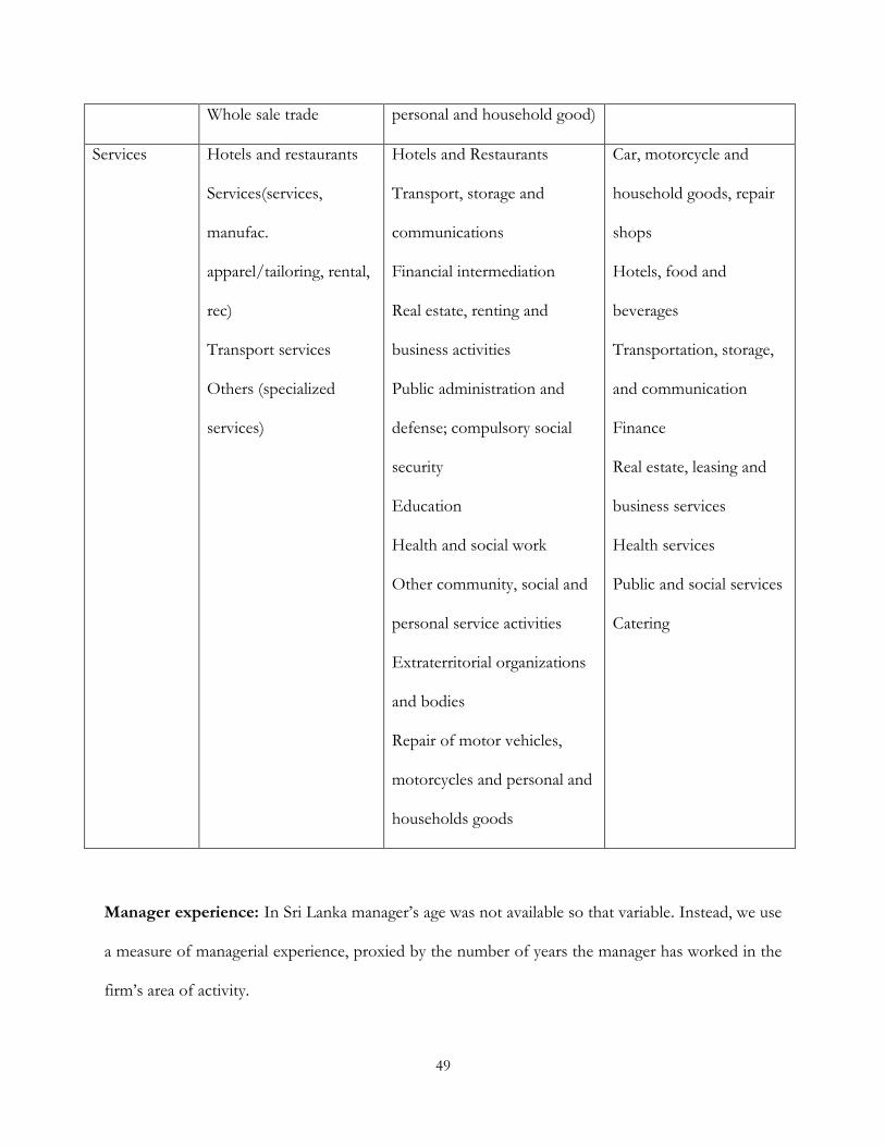
49

Whole sale trade personal and household good)

Services Hotels and restaurants

Services(services,

manufac.

apparel/tailoring, rental,

rec)

Transport services

Others (specialized

services)

Hotels and Restaurants

Transport, storage and

communications

Financial intermediation

Real estate, renting and

business activities

Public administration and

defense; compulsory social

security

Education

Health and social work

Other community, social and

personal service activities

Extraterritorial organizations

and bodies

Repair of motor vehicles,

motorcycles and personal and

households goods

Car, motorcycle and

household goods, repair

shops

Hotels, food and

beverages

Transportation, storage,

and communication

Finance

Real estate, leasing and

business services

Health services

Public and social services

Catering

Manager experience: In Sri Lanka manager’s age was not available so that variable. Instead, we use

a measure of managerial experience, proxied by the number of years the manager has worked in the

firm’s area of activity.

50

Household enterprise: This variable identifies home based firms.

Electricity usage: Dummy variable that takes the value one when the firm uses electricity and zero

otherwise.

Firm age: The age of the firm measured in years.

51

Appendix B: Key Country Characteristics

Table B1: Key Country Characteristics

Indonesia Bangladesh Sri Lanka Ethiopia

Population (million) 227.3 143.9 19.4 75.9

Rural population (% of total population) 51.9% 73.3% 84.7% 83.6%

Human Development Index 0.572 0.478 0.662 0.327

GDP per capita (current US$) 1,258 475 975 200

Poverty headcount ratio at rural poverty line (% of rural population) 20% 43.8% 24.7% 39.3% Poverty headcount ratio at urban poverty line (% of urban population) 11.7% 28.4% 7.9% 35.1%

Agriculture, value added (% of GDP) 13.1% 19.2% 13.2% 47.9%

Social Institutions and Gender Index / OECDa

0.128 0.245 0.059 0.233

Gender Inequality Index / UNDPb 0.549 0.602 0.447 -

Main religions (% of population)

Muslim 86.1%, Protestant 5.7%,

Roman Catholic 3%

Muslim 89.5%, Hindu 9.6%, other 0.9%

Buddhist 69.1%, Muslim 7.6%, Hindu 7.1%

Orthodox 43.5%, Muslim 33.9%,

Protestant 18.6%

Female Male Female Male Female Male Female Male

Life expectancy at birth (years) 68.7 65.5 68.1 67.3 77.0 69.5 57.5 54.5 Literacy rate, adult (% of population ages 15 and above) 86.8% 94.0% 51.0% 60.7% 89.1% 92.2% 18.0% 41.9%

Expected years of schooling 11.6 12.1 8.3 8.0 12.8 12.4 6.4 8.3

Labor force participation rate (% of population ages 15-64) 52% 87.6% 61% 85.9% 39.5% 81.2% 80.8% 91.6%

Employees, agriculture (% of employment) 44.3% 43.8% 68.1% 41.8% 39.2% 31.6% 74.8% 83.2%

Sources: World Development Indicators, UNDP, OECD, CIA Fact Book Years: Indonesia 2005 (2004 when not available), Bangladesh 2007 (2005 when not available), Sri Lanka 2003 (2002 when not available), Ethiopia 2006 (2005 or closest year when not available) a The SIGI was measured in 102 countries in 2009. It includes 12 indicators on social institutions, which are grouped into 5 categories: Family Code, Physical Integrity, Son Preference, Civil Liberties and Ownership Rights (0=low/no discrimination, 1=high discrimination). b The Gender Inequality Index was measured in 138 countries in 2010. The index incorporates the following indicators: Labor force participation, educational attainment, parliamentary representation, adolescent fertility and maternal mortality (higher values indicate lower achievement).

52

Appendix C: Constraints

When asked about the most important constraint to running their firm, both male and female

managers consider a lack of markets (demand), transport, access to credit and electricity as their

most important constraints, as is demonstrated in Table C1. The importance of these constraints

varies across countries. For example, concerns about markets are particularly pressing in Bangladesh

and Ethiopia. Governance and public utilities are the most burdensome constraints for a much

smaller group of firms in each country. Other constraints, such as taxation, registration procedures,

labor regulation and the availability and regulation of land are only considered the most important

constraint by very small minorities of firms in each country. Thus, gender differences in perceived

constraints and their ranking are not large in general, and, moreover, vary across countries.

Table C2 documents self-reported measures of the severity of different constraints. There

are very few constraints that are always consistently considered more of a constraint by either

gender. An exception is governance, which men always consider more of a constraint than women

(although the gender difference is not statistically significant in Indonesia), perhaps because male

firms tend to be larger. Registration, taxes and public infrastructure are considered a significantly

more severe obstacle by male managers in Bangladesh, Ethiopia and Sri Lanka, but not in Indonesia,

perhaps reflecting differences in firm size. Women consider access to finance more of a constraint in

Bangladesh, Ethiopia and Indonesia, while men consider it more of a problem in Sri Lanka.

To assess to what extent gender differences in constraints might be driven by, or masked by,

firm characteristics, we estimate ordered probit models of the severity of a given problem,

controlling for firm size, capital stock, sector, human capital of the manager, investment climate

characteristics and gender. Results are presented in Table C3. The gender dummies are most often

insignificant, and their sign varies considerably across countries. Overall, no systematic gender

53

patterns emerge. In sum, gender differences in self-reported constraints are small - both

unconditionally and conditional on differences in firm, human capital, and investment climate

characteristics.

54

Table C1: Most important constraint

Most Important Constraints Bolded coefficients indicate gender differences are statistically significant at the 5% level.

Bangladesh Ethiopia Indonesia Sri Lanka

Women Men Women Men Women Men Women Men

mean/se mean/se mean/se mean/se mean/se mean/se mean/se mean/se

electricity 0.04 0.17 0.08 0.05 0.12 0.17 0.25 0.27

0.19 0.38 0.27 0.21 0.33 0.37 0.43 0.44

public utilities 0.00 0.01 0.10 0.05 0.05 0.03 0.11 0.14 0.00 0.09 0.30 0.22 0.22 0.17 0.32 0.34

finance 0.23 0.10 0.31 0.32 0.22 0.25 0.16 0.19

0.43 0.30 0.46 0.47 0.42 0.43 0.36 0.39

transport 0.11 0.09 0.12 0.18 0.19 0.11 0.19 0.18

0.32 0.29 0.32 0.39 0.39 0.32 0.39 0.39

markets 0.50 0.43 0.37 0.36 0.24 0.28 0.27 0.14

0.50 0.50 0.48 0.48 0.43 0.45 0.45 0.35

labor 0.00 0.00 NA NA 0.00 0.00 0.01 0.02

0.00 0.03 NA NA 0.06 0.05 0.10 0.13

land 0.00 0.01 0.01 0.02 0.01 0.01 0.00 0.01

0.00 0.10 0.12 0.14 0.10 0.11 0.06 0.10

governance 0.08 0.08 0.01 0.00 0.11 0.10 0.00 0.01

0.28 0.27 0.08 0.03 0.31 0.29 0.04 0.12

registration 0.00 0.01 0.00 0.01 0.02 0.01 0.00 0.01

0.00 0.10 0.00 0.09 0.15 0.10 0.04 0.09

taxes 0.00 0.00 0.00 0.01 0.03 0.01 0.00 0.01

0.00 0.03 0.00 0.09 0.18 0.10 0.05 0.09

others 0.03 0.10 0.01 0.01 0.00 0.03 0.00 0.02 0.18 0.29 0.07 0.10 0.03 0.16 0.03 0.14

Note: Statistics are weighted.

55

Table C2: Average rating of severity of constraints

Severity of Different Constraints Bolded coefficients indicate gender differences are statistically significant at the 5% level.

Bangladesh Ethiopia Indonesia Sri Lanka

Women Men Women Men Women Men Women Men

mean/se mean/se mean/se Mean/se mean/se Mean/se mean/se mean/se

electricity 0.65 1.28 0.87 1.00 1.17 1.1 0.87 1.2

0.81 1.12 1.27 1.36 1.28 1.29 1.15 1.29

public utilities

0.00 0.06 1.21 1.06 1.03 0.79 0.62 1.01

0.06 0.37 1.33 1.35 1.3 1.18 1.01 1.24

finance 1.50 1.27 2.11 1.84 1.8 1.78 1.24 1.40

1.40 1.23 1.27 1.38 1.38 1.38 1.39 1.40

transport 1.38 1.36 1.33 1.81 1.32 1.26 1.13 1.17

0.95 1.18 1.40 1.37 1.35 1.33 1.32 1.36

markets 2.09 2.08 2.31 2.29 1.21 1.25 1.39 1.25

0.82 0.98 1.11 1.07 1.28 1.33 1.35 1.36

labor 0.02 0.03 0.15 0.47 0.5 0.49 0.11 0.2

0.16 0.23 0.63 1.04 0.99 0.99 0.56 0.72

land 0.11 0.14 0.65 0.52 0.46 0.49 0.04 0.11

0.55 0.51 1.14 1.10 0.99 0.99 0.28 0.54

governance 1.48 2.05 0.24 0.61 1.13 1.19 0.13 0.22

1.00 0.96 0.71 1.06 1.38 1.34 0.58 0.74

registration 0.00 0.11 0.03 0.22 0.62 0.61 0.08 0.17

0.06 0.38 0.24 0.71 1.09 1.07 0.49 0.66

taxes 0.00 0.02 0.10 0.47 0.68 0.65 0.07 0.15 0.05 0.18 0.45 1.04 1.11 1.12 0.44 0.62

Note: In each country managers were asked about the severity of different obstacles to investment. Constraints were grouped by theme and the maximum value of the different constraints in a given category was used as a measure of the severity of the constraint. For example, public utilities covers problems with water, telecommunication and postal services. Different country scales of severity were converted to the following common scale: 0=no problem, 1=a minor problem, 2=somewhat of a problem, 3=a major problem. Statistics are weighted.

56

Table C3: Ordered probits

Ordered Probit Models of Severity of Constraints

Dependent

Variable electricity finance transport market

public utilities

labor land governance

registration

taxes

Country Explanatory

variable coef/se coef/se coef/se coef/se coef/se coef/se coef/se coef/se coef/se coef/se

Bangladesh

mngr is male 0.276* -0.317 -0.024** 0.251 0.504 0.156 -0.109 0.548 1.093* 0.618

(0.208) (0.255) (0.214) (0.273) (0.320) (0.434) (0.487) (0.223) (0.463) (0.490)

Ethiopia mngr is male 0.237 -0.247 0.300 -0.210 -0.049 1.553*** -0.065 0.685***

0.559** 0.794**

(0.248) (0.196) (0.220) (0.270) (0.213) (0.430) (0.236) (0.204) (0.273) (0.378)

Indonesia mngr is male -0.122 -0.058 -0.058 -0.009 -0.196* -0.010 0.071 -0.049 -0.046 0.053

(0.131) (0.115) (0.133) (0.118) (0.115) (0.166) (0.134) (0.125) (0.131) (0.143)

Sri Lanka mngr is male 0.264* 0.086 0.148 -0.004 0.355***

0.162 0.214 -0.082 0.150 -0.112

(0.139) (0.143) (0.131) (0.136) (0.123) (0.196) (0.207) (0.218) (0.183) (0.182)

Controls included but not presented:

hh enterprise, services, trade, log firm age, electricity, lnK, lnL mngr age, mngr age2/100, mngr primary, mngr secondary, mngr tertiary, town, ln dist market, credit institution, ln local wage

Note: *** p<0.01, ** p<0.05, * p<0.1. Regressions are weighted. Standard errors are heteroscedasticity robust and clustered at the village level.

57

Appendix D: Probit Participation Models

Participation in Bangladesh and Ethiopia Univariate Probit Models

Bangladesh Ethiopia

Women Men Women Men Women Men Women NFE Agriculture Wage NFE Agriculture Wage

coef/se coef/se coef/se coef/se coef/se coef/se coef/se coef/se coef/se

age 0.080** -0.013 0.114*** 0.010 0.046 -0.026 0.098*** -0.021 0.114***

(0.040) (0.041) (0.041) (0.043) (0.062) (0.041) (0.023) (0.018) (0.025)

age2/100 -0.134** 0.019 -0.148*** -0.006 -0.074 0.004 -0.124*** 0.009 -0.167***

(0.054) (0.050) (0.051) (0.052) (0.080) (0.050) (0.029) (0.023) (0.033)

primary 0.095 0.276 0.405** -0.082 0.130 0.107 -0.151 0.275** -0.122

(0.169) (0.178) (0.204) (0.178) (0.259) (0.183) (0.166) (0.127) (0.173)

secondary 0.032 0.476*** 0.215 -0.142 -0.208 -0.296* -0.569** -1.063*** 1.160***

(0.189) (0.184) (0.218) (0.177) (0.306) (0.179) (0.267) (0.320) (0.271)

tertiary -0.218 0.414 -2.586*** -1.055*** 1.697*** 0.784**

(0.578) (0.359) (0.521) (0.335) (0.441) (0.341)

head 1.025*** 0.296 0.424 0.032 0.335 -0.125 0.443* 0.297 0.016

(0.341) (0.250) (0.391) (0.262) (0.548) (0.260) (0.231) (0.190) (0.234)

spouse 0.292 -0.437 0.298 -1.406*** -0.363 -0.095 -0.309 0.288* -0.980***

(0.311) (0.454) (0.330) (0.464) (0.467) (0.463) (0.244) (0.173) (0.220)

child 0.221 0.015 -0.074 -0.488** 0.200 -0.306 -0.135 -0.002 -0.128

(0.287) (0.175) (0.344) (0.216) (0.399) (0.194) (0.218) (0.179) (0.230)

married -0.554** 0.113 -1.066*** 0.470** -0.620** 0.098 -0.297 0.226 0.174

(0.266) (0.214) (0.272) (0.214) (0.310) (0.202) (0.218) (0.159) (0.204)

widow/divorced 0.097 -1.489** -0.250 -1.675** 0.152 0.740 0.061 0.429*** 0.030

(0.418) (0.610) (0.388) (0.746) (0.487) (0.751) (0.196) (0.154) (0.170)

ln hh size -0.149 -0.079 -0.218 0.354** -0.251 -0.204 -0.364*** 0.268*** -0.180

(0.204) (0.180) (0.205) (0.178) (0.250) (0.178) (0.097) (0.098) (0.130)

sh child 0.305 0.064 -0.146 0.070 -1.564** -0.158 0.392 -0.587*** 0.129

(0.408) (0.408) (0.490) (0.378) (0.626) (0.409) (0.251) (0.217) (0.289)

sh elderly 0.564 0.282 0.765 1.542 -1.132 -0.742 0.326 -0.478 -0.177

(0.852) (0.894) (0.725) (0.950) (1.014) (0.912) (0.561) (0.382) (0.635)

electricity -0.087 0.195 0.456** -0.151 0.520 -0.183 0.172 -0.557*** 0.144

(0.204) (0.226) (0.213) (0.245) (0.396) (0.232) (0.131) (0.188) (0.241)

town 0.455*** 0.807*** 0.331* -0.273* -0.182 -0.813*** 0.681*** -1.823*** 0.089

(0.157) (0.130) (0.186) (0.144) (0.244) (0.134) (0.165) (0.173) (0.222)

ln dist market 0.013 -0.068 0.057 -0.080 -0.031 -0.120 -0.363*** 0.075 0.016

(0.109) (0.100) (0.104) (0.105) (0.207) (0.098) (0.073) (0.053) (0.070)

credit institution 0.055 0.398*** 0.052 -0.024 -0.287 -0.288** 0.067 0.048 0.125

(0.163) (0.147) (0.173) (0.143) (0.256) (0.136) (0.096) (0.068) (0.102)

ln local wage -0.467* -0.418* -0.859*** -1.091*** -0.605 0.216 -0.191* -0.179** -0.066

(0.251) (0.254) (0.276) (0.268) (0.389) (0.262) (0.104) (0.091) (0.103)

partner primary 0.042 -0.240 -0.149 0.099 0.568 -0.155 0.398*** 0.002 0.084

(0.180) (0.225) (0.211) (0.193) (0.376) (0.232) (0.131) (0.088) (0.162)

partner secondary 0.004 -0.341 0.132 0.088 0.720** 0.112 0.258 -0.176 0.227

(0.245) (0.212) (0.265) (0.199) (0.360) (0.213) (0.356) (0.249) (0.284)

partner tertiary 0.129 -1.398** -0.786 0.400 0.875* 0.443

(0.432) (0.700) (0.511) (0.625) (0.490) (0.544)

h father NFE 0.261* 0.187 -0.356* -0.505*** 0.113 0.165

(0.144) (0.151) (0.200) (0.155) (0.244) (0.162)

h father wage -0.073 -0.150 -0.586*** -0.878*** 0.968*** 0.944*** (0.166) (0.154) (0.201) (0.175) (0.219) (0.152) Constant 2.557 3.927 6.535** 10.614*** 4.213 -0.941 -0.424 1.643** -2.409*** (2.557) (2.681) (2.767) (2.845) (4.141) (2.767) (0.936) (0.821) (0.889)

N 3,515 4,158 3,515 4,158 3,515 4,158 2,805 2,805 2,805 Adjusted R2 0.104 0.075 0.141 0.185 0.252 0.150 0.272 0.105 0.166

Note: *** p<0.01, ** p<0.05, * p<0.1. Regressions are weighted. Standard errors are heteroscedasticity robust and clustered at the household level

58

Participation in Indonesia and Sri Lanka Univariate probit models

Indonesia Sri Lanka

NFE Wage NFE Agriculture Wage

women men women men women men women men women men

coef/se coef/se coef/se coef/se coef/se coef/se coef/se coef/se coef/se coef/se

age 0.121*** 0.049 0.095** 0.117*** 0.066*** 0.036 0.099*** 0.046* 0.097*** 0.127***

(0.031) (0.034) (0.042) (0.031) (0.023) (0.022) (0.028) (0.027) (0.028) (0.023) age2/100 -0.142*** -0.055 -0.136** -0.167*** -0.088*** -0.038 -0.114*** -0.029 -0.142*** -0.180***

(0.037) (0.038) (0.055) (0.040) (0.029) (0.027) (0.034) (0.032) (0.036) (0.027) primary -0.323* -0.285 0.005 0.016 0.275 0.123 0.357 0.195 0.090 0.368

(0.172) (0.190) (0.201) (0.189) (0.202) (0.303) (0.240) (0.272) (0.219) (0.260) secondary -0.076 -0.187 0.015 -0.138 0.151 0.639** 0.244 0.032 0.076 0.283

(0.175) (0.206) (0.229) (0.218) (0.195) (0.295) (0.234) (0.264) (0.212) (0.249) tertiary 0.087 -0.248 1.080*** 0.232 -0.185 -0.240 0.096 -0.596 1.097*** 1.117***

(0.270) (0.266) (0.272) (0.239) (0.371) (0.473) (0.520) (0.444) (0.370) (0.411) head 1.179*** 0.565** -0.209 0.918** 0.759*** 0.423 1.242*** 0.445 -0.163 0.484*

(0.318) (0.268) (0.301) (0.357) (0.246) (0.314) (0.373) (0.353) (0.246) (0.291) spouse -0.170 -0.111 0.610* 0.790 0.556* -1.049** 0.679* -0.883* -0.067 1.550***

(0.297) (0.528) (0.337) (0.714) (0.293) (0.496) (0.398) (0.511) (0.329) (0.435) child -0.095 0.173 -0.236 0.723** 0.144 -0.002 0.512 0.084 0.073 0.496*

(0.234) (0.275) (0.304) (0.295) (0.237) (0.269) (0.374) (0.322) (0.274) (0.281) married 0.299 0.526* 0.142 -0.113

(0.212) (0.301) (0.228) (0.233) widow/divorced -0.131 -0.175 0.714** 0.247

(0.295) (0.350) (0.341) (0.347) ln hh size 0.198 -0.011 -0.156 -0.136 0.060 0.191 -0.025 -0.438*** -0.131 -0.048

(0.122) (0.139) (0.155) (0.178) (0.129) (0.132) (0.131) (0.132) (0.128) (0.116) sh child -0.475 -0.043 -0.816** 0.504 -0.526* 0.204 0.548* 0.366 -0.746** -0.013

(0.303) (0.394) (0.396) (0.408) (0.272) (0.269) (0.282) (0.283) (0.298) (0.255) sh elderly -0.849* -0.679 0.523 0.948* -0.764 -0.314 1.059** 0.308 -0.256 0.289

(0.481) (0.619) (0.590) (0.570) (0.485) (0.427) (0.496) (0.449) (0.450) (0.418) electricity 0.302 0.859*** -0.464 -0.020 0.278 0.315 -0.549** -0.572*** 0.141 0.300

(0.225) (0.262) (0.304) (0.274) (0.236) (0.196) (0.214) (0.204) (0.216) (0.205) town 0.260** 0.194 0.257** 0.154

(0.121) (0.119) (0.124) (0.129) ln dist market -0.127** -0.005 -0.121** -0.253*** -0.059 0.036 -0.097* 0.197*** 0.080* -0.116**

(0.056) (0.049) (0.060) (0.064) (0.050) (0.050) (0.056) (0.049) (0.048) (0.046) credit institution 0.100 0.256** 0.258** -0.105 0.188** 0.267*** -0.295*** -0.232*** 0.060 -0.017

(0.112) (0.122) (0.128) (0.137) (0.085) (0.082) (0.095) (0.087) (0.087) (0.077) ln local wage -0.050 -0.171 -0.272** 0.018 0.264 0.334* -0.019 -0.237 -0.151 -0.274*

(0.130) (0.143) (0.131) (0.166) (0.183) (0.182) (0.207) (0.182) (0.200) (0.163) partner primary 0.427** 0.012 -0.384 0.107 -0.193 0.233 0.056 0.051 -0.369 0.131

(0.207) (0.172) (0.242) (0.208) (0.224) (0.208) (0.248) (0.210) (0.287) (0.197)

partner secondary 0.404** -0.085 -0.635** -0.050 -0.046 0.315* 0.106 0.085 -0.324 -0.225

(0.205) (0.194) (0.259) (0.216) (0.213) (0.191) (0.236) (0.198) (0.279) (0.183) partner tertiary 0.350 0.044 -0.478 0.193 -0.572 0.611 -0.296 0.260 0.265 -0.337

(0.275) (0.270) (0.320) (0.296) (0.459) (0.485) (0.665) (0.450) (0.518) (0.428)

h father NFE 0.260** 0.494*** -0.259 -0.177 0.125 0.292*** -0.585*** -0.625*** 0.053 0.013

(0.131) (0.160) (0.176) (0.167) (0.104) (0.102) (0.136) (0.105) (0.110) (0.098) h father wage -0.186 -0.205 0.624*** 0.535*** 0.013 -0.005 -0.417*** -0.627*** 0.415*** 0.341***

(0.167) (0.144) (0.143) (0.155) (0.107) (0.101) (0.112) (0.104) (0.103) (0.093) h father other -0.003 -0.311 -0.485 -0.279 0.119 0.271

(0.304) (0.269) (0.340) (0.324) (0.248) (0.232) constant -3.627* -0.883 2.178 -2.634 -5.581*** -6.680*** -2.769 1.740 -0.737 0.167 (1.988) (2.208) (2.136) (2.720) (2.106) (2.095) (2.418) (2.105) (2.256) (1.888) Observations 3,629 3,606 3,629 3,60

6

1,359 1,350 1,359 1,350 1,359 1,350

Pseudo R2 0.134 0.146 0.173 0.12

8

0.045 0.118 0.111 0.186 0.085 0.072 Note: *** p<0.01, ** p<0.05, * p<0.1. Regressions are weighted, except for Sri Lanka where household weights are not available. Standard errors are heteroscedasticity robust and clustered at the household level

59

Appendix E: Additional Robustness Check

As an additional robustness check we examine whether there are gender differences in the returns to

human capital, gender differences in the impact of firm characteristics and the investment climate,

and sector-specific gender productivity differentials. To assess these possibilities we interact total

factor productivity determinants term with a dummy for a female entrepreneur, The model thus

becomes:

(E1)

Under the null hypotheses of no differences in returns, all the gender interaction terms

should be equal to zero ( . There are various alternative hypotheses. For

example, women may have lower returns to schooling. In this case we would expect the interaction

terms between the gender dummy and our proxies to be negative. Alternatively, women may benefit

less from access to finance, in which case one might expect the coefficient on the gender-credit

institution interaction to be statistically significant.

Results are presented in Table E1. Gender interaction terms add very little explanatory

power; the R2s do not increase very much compared with specifications that do not include gender

interactions (see Table 5). With the exception of Bangladesh, where the sample of female firms is

very small, gender interaction terms are not in general statistically significant, either individually or

jointly. Nonetheless, there is some evidence that female enterprises that are household based in Sri

Lanka are significantly more productive than household-based male firms and that there is a positive

correlation between local wages and the productivity of male firms, but not that of female firms. In

addition, age productivity profiles for female entrepreneurs in Indonesia may be different from

those of their male counterparts. However some differences are to be expected with so many

60

interactions terms and, moreover, few differences are qualitatively similar in all countries under

consideration. Overall, the evidence for the hypotheses that the returns to human capital and the

impact of investment climate factors varies by gender is limited.

61

Table E1: Production function robustness check

Production functions – Robustness Check

Bangladesh Ethiopia Indonesia Sri Lanka

coef se coef se coef se coef se

manuf*lnK 0.065*** (0.019) 0.064* (0.036) 0.014 (0.020) -0.024 (0.058)

manuf*lnL 0.217*** (0.029) 0.421*** (0.117) 0.367*** (0.121) 0.396*** (0.104) manuf*lnM 0.670*** (0.026) 0.470*** (0.075) 0.544*** (0.099) 0.747*** (0.057) serv*lnK 0.075*** (0.012) 0.111* (0.064) 0.046** (0.018) 0.132*** (0.045) serv*lnL 0.378*** (0.045) 0.579 (0.454) 0.252*** (0.076) 0.289 (0.187) serv*lnM 0.518*** (0.020) 0.259** (0.104) 0.545*** (0.036) 0.620*** (0.066) trade*lnK 0.003 (0.012) 0.051 (0.042) 0.011 (0.014) 0.028 (0.028) trade*lnL 0.151*** (0.036) 0.628*** (0.154) 0.073* (0.044) 0.142 (0.099) trade*lnM 0.820*** (0.028) 0.519*** (0.100) 0.752*** (0.035) 0.864*** (0.031) Services 0.997*** (0.220) 0.871* (0.471) -0.196 (0.771) 0.008 (0.667) Trade -0.871*** (0.278) 0.017 (0.674) -1.524** (0.766) -1.177* (0.685) hh enterprise -0.270*** (0.045)

-0.314*** (0.108) -0.244** (0.099)

mngr age 0.003 (0.006) -0.019 (0.043) -0.028 (0.019) 0.010 (0.011) mngr age2/100 -0.363 (0.590) 0.003 (0.039) 0.029 (0.020) -0.025 (0.031) mngr primary 0.071* (0.042) -0.702*** (0.209) -0.173 (0.119) -0.110 (0.211) mngr secondary 0.053 (0.046) -0.436 (0.580) -0.008 (0.171) -0.084 (0.197) mngr tertiary 0.127** (0.050)

0.205 (0.201) -0.168 (0.230)

electricity usage 0.106*** (0.036) 0.929** (0.433) 0.076 (0.090) -0.146 (0.101) ln firm age 0.028*** (0.010) 0.069 (0.096) 0.125*** (0.044) 0.062 (0.045) Town 0.010 (0.027) 0.527 (0.324) 0.082 (0.082)

ln dist market -0.040 (0.031) 0.080 (0.129) -0.003 (0.056) 0.004 (0.053) Bank -0.039 (0.029) 0.075 (0.257) -0.037 (0.093) 0.010 (0.104) ln local wage 0.173** (0.080) 0.281 (0.210) 0.125* (0.071) 0.353** (0.168) fem*hh ent 0.084 (0.280)

0.178 (0.151) 0.339** (0.134)

fem*mngrage -0.064 (0.052) 0.042 (0.053) 0.045 (0.032) 0.019 (0.036) fem*mngrage2/100 6.587 (6.686) -0.037 (0.052) -0.058* (0.033) -0.068 (0.121) fem*primary -0.692*** (0.212) 0.259 (0.430) 0.134 (0.204) 0.237 (0.266) fem*secondary -0.680** (0.315) 1.059 (0.672) -0.010 (0.231) 0.408 (0.308) fem*tertiary -0.700** (0.345)

0.146 (0.364) 0.519 (0.525)

fem*electricity usage 0.379 (0.280) -0.308 (0.493) -0.145 (0.132) 0.227 (0.178) fem*lnfirmage -0.140 (0.121) 0.023 (0.131) -0.034 (0.059) 0.010 (0.071) fem*town 0.307* (0.174) -0.193 (0.455) -0.060 (0.137)

fem*lndistmarket -0.254 (0.185) -0.135 (0.188) 0.007 (0.067) 0.065 (0.102) fem*credit inst -0.303* (0.156) 0.306 (0.391) 0.055 (0.150) 0.147 (0.118) fem*ln localwage 0.196** (0.085) -0.220 (0.149) -0.059 (0.048) -0.080** (0.034) F TESTS – CRS

CRS-Manufacturing F(1, 154) = 3.54 F(1, 111) = 0.12 F(1, 130) = 0.39 F(1, 125) = 3.14 p>F 0.0618

0.7321

0.5353 0.0790

CRS-Services F(1, 154) = 0.56 F(1, 111) = 0.01 F(1, 130) = 5.18 F(1, 125) = 0.07 p>F 0.4572

0.9142

0.0245 0.7940

CRS-Trade F(1, 154) = 0.71 F(1, 111) = 1.28 F(1, 130) = 18.25 F(1, 125) = 0.11 p>F 0.4020

0.2598

0.0000 0.7461

F TESTS –Female

interactions

Schooling F(3, 154) = 3.67 F(2, 111) = 1.39 F(3, 130) = 0.47 F(3, 125) = 0.68 p>F 0.0137

0.2528

0.7026 0.5679

Age F(2, 154) = 1.90 F(2, 111) = 0.36 F(2, 130) = 2.82 F(2, 125) = 0.16 p>F 0.1529

0.6969

0.0636 0.8508

Investment Climate F(4, 154) = 3.79 F(4, 111) = 0.81 F(4, 130) = 0.44 F(3, 125) = 2.78 p>F 0.0057

0.5191

0.7823 0.0441

Other Firm

characteristics

F(3, 154) = 0.73 F(2, 111) = 0.20 F(3, 130) = 1.60 F(3, 125) = 2.25 p>F 0.5379

0.8169

0.1932 0.0858

All F(12, 154) = 9.66 F(10,111) = 2.24 F(12, 130) = 2.04 F(11, 125) = 1.23 p>F 0.0000

0.0205

0.0253 0.2757

Observations 1993

476

1,229 943 R2 0.965

0.575

0.814 0.825

Adjusted R2 0.964

0.546

0.809 0.819 Note: *** p<0.01, ** p<0.05, * p<0.1. Regressions are weighted. Standard errors are heteroscedasticity robust and clustered at the village level.

62

Appendix F: Investment and Growth Differentials

F.1 Gender differences in dynamic performance are small

Gender differences in the dynamic performance of firms are small and much less pronounced than

the productivity differences discussed in section 5. As shown in Table 4, investment rates are low in

Ethiopia and Bangladesh, but substantial in Indonesia and Sri Lanka. Growth rates are low in all

countries. Male managers are not significantly more likely to invest than female ones in any country.

In fact, in Sri Lanka, they are significantly less likely to invest than female managers. Male firms also

do not grow faster than female firms on average. However, the absence of large differences in

absolute growth and investment rates may obscure gender differences as they may reflect other firm

characteristics correlated with gender that impact dynamic performance. To assess whether this is

the case, investment and growth models are estimated.

F.2 Empirical Strategy

Investment is modeled by means a probit for having invested using as explanatory variables

sector, firm-, manager- and investment climate characteristics. Information on the total amount

invested because was not available in all surveys and, moreover, noisy, rendering it difficult to

examine gender differences in the intensive investment margin. As in section 5 we progressively add

explanatory variables to assess to what extent firm and investment climate characteristics account for

gender differences in investment rates. Our most general reduced-form investment model is:

(F1)

We use the same model to analyze growth, using as dependent variable the change in employment

over the average firm-size for two periods: H = (Lt -Lt-1)/[0.5*(Lt + Lt-1)], following Davis and

Haltiwanger (1992, 1999). This measure bounds the growth rate between -2 and +2 and minimizes

the impact of measurement error and influential outliers. That is our estimable equation is:

63

(F2)

where u is a zero-mean error term.

The results of these regressions have to be interpreted cautiously. Suppose, for example, that

the presence of credit institutions is positively correlated with investment rates. This might indicate

that firms with better access to financial institutions are likely to invest more. However, it is also

possible that credit institutions locate in communities where the local economy is buoyant. Thus, we

have to be aware of potential reverse causality. In addition, it is important to emphasize that

estimated coefficients are conditional on firm survival.

F.3 Results

Results are presented in tables F1 and F2. We first condition on lagged size and sector to account

for sorting effects and subsequently add additional controls for firm characteristics, managerial

human capital and the investment climate.

Starting with the results for investment which are presented in table F1, controlling for

lagged size and sector (model 2) renders the investment differentials between male and female firms

insignificant in all countries. Adding a full set of controls (model 3) does not overturn these results,

although male-firms in Indonesia are some 38% less likely to invest, ceteris paribus, and this effect is

significant at the 10%, but not the 5% level. Overall, investment is difficult to predict, as is

evidenced by the rather low pseudo R2s and the fact that relatively few explanatory variables are

significant. Moreover, the determinants of investment appear to vary substantially across countries;

not a single explanatory variable is consistently statistically significant in each country.

The results of our growth regressions are presented in table F2. Once we control for

sorting by sector and size firms run by Bangladeshi men grow faster than firms run by Bangladeshi

64

women. Yet after also including managerial, enterprise and investment climate controls gender

growth differentials are not statistically significant in any of the other countries considered.

Our models for growth also have very limited explanatory power, as is indicated by the very

low R2s. However, the determinants of firm growth do not appear to vary as dramatically across

countries as the determinants of investment and productivity. While the parameter estimates are not

always statistically significant in each country, they suggest that, overall, firms that were larger to

start with appear to have grown less. This finding presumably partly reflects measurement error and

survivor bias, as one may expect firms that started large to be more likely to survive. In addition,

manufacturing firms appear to grow somewhat faster than firms engaged in services or trade. Firm

growth also appears positively correlated with electricity usage and negatively associated with firm

age, although these patterns are not statistically significant in each country.

In short, gender differences in investment and growth rates are small and typically

insignificant, a finding which is robust to controlling for a rich set of firm, manager and investment

climate characteristics.

65

Table F1: Investment Probit

Investment Probit - Marginal Effects

Bangladesh Ethiopia Indonesia Sri Lanka

coef se coef se coef se coef se

MODEL 1: GENDER ONLY mngr is male 0.299 (0.217) 0.183 (0.130) -0.001 (0.133) -0.252** (0.128)

Observations 2,480

649

1,369

1,315

Pseudo R2 0.003

0.004

0.000

0.005

MODEL 2: GENDER, INITIAL SIZE AND SECTOR mngr is male 0.021 (0.242) 0.228 (0.150) -0.274 (0.220) -0.198 (0.150) ln Lt-1 0.164** (0.076) 0.263** (0.103) 0.187 (0.123) -0.050 (0.087)

services 0.002 (0.181) 0.157 (0.326) -0.388 (0.238) -0.343** (0.162)

trade -0.452*** (0.148) -0.002 (0.320) -0.029 (0.279) -0.106 (0.134)

hh enterprise -0.347* (0.193) 0.228 (0.150) -0.215 (0.249) 0.085 (0.139)

Observations 2,301

648

776

1,128

Pseudo R2 0.037

0.032

0.040

0.016

MODEL 3: ALL CONTROLS mngr is male -0.181 (0.259) 0.291 (0.237) -0.378* (0.204) -0.074 (0.136) ln Lt-1 0.181* (0.093) 0.142 (0.087) 0.220* (0.117) 0.075 (0.098)

services -0.034 (0.193) 0.243 (0.304) -0.610** (0.302) -0.289* (0.168)

trade -0.436*** (0.168) -0.021 (0.276) -0.182 (0.278) -0.086 (0.139)

hh enterprise -0.397* (0.225)

-0.071 (0.288) 0.086 (0.139)

mngr age -0.017 (0.031) -0.008 (0.043) 0.122*** (0.043) -0.000 (0.016)

mngr age2/100 1.477 (3.654) -0.000 (0.043) -0.142*** (0.048) -0.003 (0.052)

mngr primary -0.172 (0.231) 0.144 (0.208) -0.457 (0.330) -0.396 (0.513)

mngr secondary -0.204 (0.209) 0.294 (0.251) 0.037 (0.284) -0.375 (0.513)

mngr tertiary -0.108 (0.417)

-0.426 (0.472) -0.393 (0.634)

electricity usage 0.325 (0.206) 1.227*** (0.243) 0.144 (0.251) 0.196* (0.110)

ln firm age 0.039 (0.075) 0.191*** (0.070) -0.029 (0.119) -0.151*** (0.054)

town 0.055 (0.148) -0.137 (0.286) 0.384 (0.248)

ln dist market 0.430*** (0.163) -0.155 (0.152) 0.005 (0.102) -0.024 (0.092)

credit institution 0.240 (0.177) -0.388 (0.273) 0.224 (0.279) 0.091 (0.152)

ln local wage -0.482 (0.299) -0.043 (0.278) 0.626** (0.262) -1.574*** (0.334)

Observations 1,855

574

697 993

Pseudo R2 0.069

0.106

0.152 0.073

Note: *** p<0.01, ** p<0.05, * p<0.1. Regressions are weighted. Standard errors are heteroscedasticity robust and clustered at the village level.

66

Table F2: Growth Models

Growth Models

Bangladesh Ethiopia Indonesia Sri Lanka

coef se coef se coef se coef se

MODEL 1: GENDER ONLY mngr is male 0.013 (0.010) 0.085 (0.058) 0.008 (0.041) -0.006 (0.012)

Observations 2,301

725

776

1,130

R2 0.000

0.009

0.000

0.001

Adjusted R2 0.000

0.008

-0.001

-0.000

MODEL 2: GENDER, INITIAL SIZE AND SECTOR mngr is male 0.054*** (0.013) 0.075 (0.051) 0.038 (0.034) -0.004 (0.011) ln Lt-1 -0.047*** (0.011) -0.132*** (0.029) -0.030 (0.045) -0.018* (0.010)

services -0.065*** (0.022) -0.057 (0.046) 0.070 (0.053) -0.019 (0.015)

trade -0.096*** (0.020) -0.041 (0.049) 0.080 (0.055) -0.013 (0.014)

hh enterprise -0.059*** (0.020)

-0.082 (0.058) -0.005 (0.012) Observations observations

2,301

724

776

1,128

R2 0.046

0.116

0.026

0.015

Adjusted R2 0.044

0.112

0.020

0.010

MODEL 3: ALL CONTROLS mngr is male 0.055*** (0.015) 0.077 (0.063) 0.017 (0.031) -0.001 (0.012) ln Lt-1 -0.046*** (0.012) -0.159*** (0.034) -0.041 (0.043) -0.020* (0.011) services -0.055*** (0.020) -0.071* (0.040) 0.044 (0.060) -0.026 (0.018)

trade -0.095*** (0.023) -0.085 (0.057) 0.076 (0.063) -0.018 (0.016)

hh enterprise -0.041** (0.019)

-0.064 (0.070) 0.003 (0.012)

mngr age 0.001 (0.002) 0.013* (0.008) 0.020* (0.012) -0.003** (0.001)

mngr age2/100 -0.146 (0.212) -0.012 (0.009) -0.020* (0.011) 0.006* (0.003)

mngr primary 0.004 (0.013) 0.047 (0.059) -0.016 (0.038) -0.003 (0.016) mngr secondary -0.004 (0.015) 0.151** (0.075) 0.041 (0.042) 0.010 (0.018)

mngr tertiary 0.055* (0.033)

0.024 (0.075) 0.015 (0.024)

electricity usage 0.024* (0.012) 0.063 (0.088) 0.126**

*

(0.038) 0.005 (0.012)

ln firm age -0.014*** (0.005) -0.017 (0.018) 0.022 (0.029) 0.000 (0.005)

town -0.018 (0.011) 0.096* (0.058) 0.031 (0.029)

ln dist market 0.016* (0.008) -0.027 (0.022) 0.015 (0.014) -0.009 (0.006) credit institution 0.007 (0.008) 0.001 (0.042) 0.030 (0.036) 0.009 (0.010)

ln local wage 0.038** (0.016) -0.035 (0.048) 0.046* (0.027) 0.031 (0.021)

Observations 1,855

636

697 993

R2 0.064

0.170

0.121 0.045

Adjusted R2 0.056

0.152

0.100 0.030

Note: *** p<0.01, ** p<0.05, * p<0.1. Regressions are weighted, except for Sri Lanka where weights are not available. Standard errors are heteroscedasticity robust and clustered at the village level