Gemma Cadby - UWA Research Repository€¦ · The genetic epidemiology of melanoma susceptibility...
376
The genetic epidemiology of melanoma susceptibility and prognosis and investigations of causal pathway modelling in complex disease aetiology. Gemma Cadby Bachelor of Science (Honours) This thesis is presented for the degree of Doctor of Philosophy of The University of Western Australia School of Population Health. May, 2011
Transcript of Gemma Cadby - UWA Research Repository€¦ · The genetic epidemiology of melanoma susceptibility...

The genetic epidemiology of melanoma
susceptibility and prognosis and investigations of
causal pathway modelling in complex disease
aetiology.
Gemma Cadby
Bachelor of Science (Honours)
This thesis is presented for the degree of
Doctor of Philosophy
of The University of Western Australia
School of Population Health.
May, 2011

ii

i
Declaration
This thesis is the author’s own composition. All sources have been acknowledged
and the author’s contribution is clearly identified in this thesis. This thesis con-
tains published work and/or work prepared for publication, some of which has
been co-authored. The permission of all co-authors has been obtained to include
the work in this thesis.
For work which has been prepared for publication, the work performed by the
author of this thesis has been described in detail.
This thesis was completed during the course of enrolment in this degree at the
University of Western Australia and has not previously been accepted for a degree
at this or another institution.

ii

iii
Abstract
Genetic epidemiological studies are increasingly being used to investigate the role
of genetic and environmental factors in common human disease aetiology, with the
ultimate aims of control and prevention. This thesis investigated the association
of candidate genes with melanoma susceptibility and prognosis in the Western
Australian population. In addition, methods research into novel statistical meth-
ods to model causal pathways in epidemiological studies was undertaken.
Australia has the highest incidence of cutaneous malignant melanoma in the world.
Several melanoma-susceptibility genes have been identified, however a greater un-
derstanding of these genes and their interactions with environmental factors would
lead to better interventions and control of the disease. The genetic determinants
of melanoma progression, and therefore prognosis, are largely unknown. Knowl-
edge of the genes which affect melanoma progression and prognosis would aid
in identifying individuals at risk of poorer prognosis, and may also elucidate the
mechanisms underlying melanoma progression. The collection of population-based
clinical, phenotypic and genetic data is integral in facilitating investigation into
the genetic and environmental factors affecting melanoma susceptibility and prog-
nosis.
This thesis involved the establishment of the Western Australian Melanoma Health
Study (WAMHS). The WAMHS is a population-based case-collection and linked
biospecimen resource established to investigate the genetic epidemiology of melanoma.
All eligible Western Australian adult cases of melanoma, diagnosed between Jan-
uary 2006 and September 2009 and notified to the Western Australian Cancer Reg-

iv
istry (WACR), were invited to participate in the study. Clinical and questionnaire-
based phenotypic data and blood samples for extraction of DNA, RNA and serum
were collected from consenting cases. Clinical data consisted of all pathological
data recorded by the WACR and the questionnaire covered major risk factors
for melanoma, such as sun exposure history and pigmentation. The final sample
consisted of 1,643 cases, of which 1,455 completed one or more components of
the study and 1,157 completed all components. The WAMHS comprises the only
population-based study of melanoma cases in Western Australia, and is one of the
largest single studies in the world.
A sub-sample of the WAMHS consisting of 800 European-ancestry participants
was used to investigate the genetic epidemiology of melanoma susceptibility and
melanoma prognosis. The genetic epidemiology of melanoma susceptibility was
investigated through association analyses of 42 single nucleotide polymorphisms
(SNPs) in genes previously reported to be associated with melanoma-risk, com-
paring the WAMHS sample to two general population samples. The genetic epi-
demiology of melanoma prognosis was investigated by association analyses of these
same SNPs with Breslow thickness, which is the best independent predictor for
disease prognosis. I hypothesised that some of the genes which increase melanoma-
risk may also be those which affect poorer disease prognosis, as reflected by in-
creased Breslow thickness.
As a result of this study, 14 SNPs in nine candidate genes were found to be
associated with melanoma-risk. The associations between six of these SNPs
(MC1R rs258322, TYR rs1393350, IRF4 rs12203592, MTAP rs7023329, MTAP
rs1011970 and BRAF rs6944385) remained significant after adjusting for multiple

v
testing. Four SNPs (IRF4 rs12203592, OCA2 rs1800401, TP53 rs1042522 and
BRAF rs1733826) were found to be associated with Breslow thickness. However,
none of these associations remained significant after adjustment for multiple test-
ing. The IRF4 rs12203592 SNP was associated with increased melanoma-risk and
thicker Breslow thickness, and therefore poorer prognosis. In addition, epidemio-
logical analyses of melanoma prognosis identified two phenotypic variables – age
at diagnosis and presence of naevi – which were associated with Breslow thickness.
In the second section of this thesis, I describe a statistical method known as
Mendelian randomisation, which is used to infer causal relationships between po-
tentially modifiable environmental exposures and some disease trait, using genetic
variants. More certain inferences regarding causal associations in epidemiological
studies are important as it may identify modifiable risk factors, i.e. information
that would allow individuals to modify their behaviours and exposures in order
to reduce the risk of some disease outcome.
As part of the methods work, I have developed an R library – MRsnphap – which
can be used to apply Mendelian randomisation to the genetic epidemiological set-
ting, by using SNPs and haplotypes as proxy variables for modifiable exposures.
While the use of SNPs as instruments is straightforward, the use of haplotypes
is not due to the uncertainty of haplotype phase. MRsnphap is the first soft-
ware for Mendelian randomisation analysis designed specifically for the genetic
epidemiological setting, which is able to incorporate the uncertainty surrounding
haplotypes into the analysis.

vi
The collection and analysis of population-based genotypic and phenotypic data
is integral in understanding the aetiology of disease. This is a critical step which
will enable the clinical utilisation of new knowledge and tools to improve clinical
practice and public health. The research presented in this thesis is both novel
and significant as it includes the first known study of the genetic determinants
of melanoma in a Western Australian population. This thesis also presents the
first comprehensive investigation into the role of candidate loci and melanoma
prognosis in a large, well-characterised sample of European-ancestry melanoma
cases. In addition, the availability of MRsnphap will help further elucidate the
role between modifiable exposures and disease, so that interventions can occur to
reduce the impact of disease in the community.

vii
Publications
Publications arising directly from this thesis
G. Cadby, S.V. Ward, (joint first authors), A. Lee, J.M. Cole, J. Heyworth,
M. Millward, T. Threlfall, F. Wood and L.J. Palmer. The Western Australian
Melanoma Health Study: Study design and participant characteristics. [IN PRESS:
CANCER EPIDEMIOLOGY]
G. Cadby, P.A. McCaskie and L.J. Palmer. (1923T). Mendelian Randomisation :
Modelling single SNPs and haplotypes in R. Presented at the 59th Annual Meeting
of The American Society of Human Genetics, October 24, 2009, Honolulu, Hawaii.
Available at http://www.ashg.org/2009meeting/abstracts/fulltext/. [ABSTRACT]
G. Cadby, S.V. Ward, J.M. Cole, M. Millward and L.J. Palmer. Breslow
thickness in the Western Australian Melanoma Health Study. Pigment Cell and
Melanoma Research, 22(6):903–904, 2009. [ABSTRACT]
S.V. Ward, G. Cadby, J.M. Cole, F. Wood, M. Millward and L.J. Palmer. The
Western Australian Melanoma Health Study. Genetic Epidemiology, 33:787, 2009.
[ABSTRACT]
L. Simpson, M. Cooper, G. Cadby, A.C. Fedson, K.L. Ward, J.D Lee, B. Szeg-
ner, C. Edwards, S. Mukherjee, D.R. Hillman, P. Eastwood and L.J. Palmer. Use
of the fat mass and obesity associated (FTO:RS9939609) single nucleotide poly-

viii
morphism to investigate the relationship between obesity and obstructive sleep
apnoea. Sleep and Biological Rhythms, 7:A18–19, 2009. [ABSTRACT]
M. Cooper, G. Cadby, J.D. Lee, A.C. Fedson, L. Simpson, K.L. Ward, D.R.
Hillman, S. Mukherjee and L.J. Palmer. Using Mendelian Randomisation to in-
vestigate the relationship between blood pressure and the severity of obstructive
sleep apnoea. Genetic Epidemiology, 33:778, 2009. [ABSTRACT]
G. Cadby, S.V. Ward, J.M. Cole, M. Millward and L.J. Palmer. Association
of candidate SNPs with melanoma susceptibility in Australian adults. Genetic
Epidemiology, 34(8):917-992, 2010. [ABSTRACT]
Publications not arising directly from this thesis
G. Cadby, K.W. Carter, S. Wiltshire and L.J. Palmer. Investigating aspects
of statistical power in meta–analysis of complex traits. Genetic Epidemiology,
33:791, 2009. [ABSTRACT]
S.V. Ward, G. Cadby, M. Millward, J.M. Cole, F. Wood and L.J. Palmer.
Scar outcome post melanoma excision. Pigment Cell and Melanoma Research,
22(6):903–904, 2009. [ABSTRACT]

ix
Contents
Declaration i
Abstract iii
Publications vii
Contents ix
List of Tables xviii
List of Figures xx
Glossary xxiii
Abbreviations xxvii
Acknowledgements xxix
Preface xxxi
1 Introduction 1
1.1 Introduction to Epidemiology . . . . . . . . . . . . . . . . . . . . 1
1.1.1 Causality in epidemiology . . . . . . . . . . . . . . . . . . 2
1.2 Introduction to Genetic Epidemiology . . . . . . . . . . . . . . . . 3
1.3 Genetic Concepts and Definitions . . . . . . . . . . . . . . . . . . 5
x
1.3.1 Genes and alleles . . . . . . . . . . . . . . . . . . . . . . . 5
1.3.2 Genetic variation . . . . . . . . . . . . . . . . . . . . . . . 7
1.3.2.1 Single nucleotide polymorphisms . . . . . . . . . 8
1.3.2.2 Haplotypes . . . . . . . . . . . . . . . . . . . . . 10
1.3.2.3 Haplotype inference . . . . . . . . . . . . . . . . 12
1.3.3 Hardy-Weinberg equilibrium principle . . . . . . . . . . . . 13
1.3.4 Linkage disequilibrium . . . . . . . . . . . . . . . . . . . . 14
1.4 Gene Discovery in Human Disease . . . . . . . . . . . . . . . . . . 15
1.4.1 Simple and complex disease . . . . . . . . . . . . . . . . . 16
1.4.2 Linkage analysis . . . . . . . . . . . . . . . . . . . . . . . . 17
1.4.3 Genetic association studies . . . . . . . . . . . . . . . . . . 18
1.4.4 Multiple testing . . . . . . . . . . . . . . . . . . . . . . . . 19
1.5 Aims . . . . . . . . . . . . . . . . . . . . . . . . . . . . . . . . . . 20
1.6 Outline of thesis . . . . . . . . . . . . . . . . . . . . . . . . . . . . 21
2 Genetic Epidemiology of Malignant Melanoma: Susceptibility
and Prognosis in the WAMHS 23
2.1 Introduction . . . . . . . . . . . . . . . . . . . . . . . . . . . . . . 23
2.2 Literature Review . . . . . . . . . . . . . . . . . . . . . . . . . . . 24
2.2.1 Skin cancer . . . . . . . . . . . . . . . . . . . . . . . . . . 24
2.2.2 Melanoma biology . . . . . . . . . . . . . . . . . . . . . . 25
2.2.3 Melanoma incidence and mortality . . . . . . . . . . . . . 27
2.2.3.1 Melanoma in Australia . . . . . . . . . . . . . . . 27
2.2.3.2 Melanoma in Western Australia . . . . . . . . . . 34
2.2.4 The aetiology of malignant melanoma . . . . . . . . . . . . 36
2.2.4.1 Environmental and host melanoma risk factors . 36
2.2.4.1.1 Sun exposure . . . . . . . . . . . . . . . 36
xi
2.2.4.1.2 Skin type and pigmentation . . . . . . . 39
2.2.4.1.3 Family history . . . . . . . . . . . . . . 41
2.2.4.1.4 Naevi . . . . . . . . . . . . . . . . . . . 42
2.2.4.2 Melanoma genetic risk factors . . . . . . . . . . . 43
2.2.4.2.1 High penetrance melanoma-susceptibility
genes . . . . . . . . . . . . . . . . . . . . 43
2.2.4.2.2 Low penetrance melanoma-susceptibility
genes . . . . . . . . . . . . . . . . . . . . 45
2.2.5 The diagnosis and treatment of melanoma . . . . . . . . . 49
2.2.6 Breslow thickness . . . . . . . . . . . . . . . . . . . . . . . 50
2.2.6.1 Breslow thickness and prognosis . . . . . . . . . . 50
2.2.6.1.1 Breslow thickness and melanoma risk fac-
tors . . . . . . . . . . . . . . . . . . . . 52
2.2.7 Literature Review Summary . . . . . . . . . . . . . . . . . 54
2.3 The Western Australian Melanoma Health Study . . . . . . . . . 56
2.3.1 Author’s contribution . . . . . . . . . . . . . . . . . . . . . 56
2.3.2 Introduction . . . . . . . . . . . . . . . . . . . . . . . . . . 56
2.3.3 WAMHS population . . . . . . . . . . . . . . . . . . . . . 57
2.3.3.1 Recruitment . . . . . . . . . . . . . . . . . . . . . 59
2.3.3.2 WAMHS pilot study . . . . . . . . . . . . . . . . 62
2.3.3.3 WAMHS full-scale implementation I . . . . . . . 64
2.3.3.4 WAMHS full-scale implementation II . . . . . . . 66
2.3.3.5 Biospecimens . . . . . . . . . . . . . . . . . . . . 67
2.3.3.6 Study variables . . . . . . . . . . . . . . . . . . . 68
2.3.3.6.1 Phenotypic variables . . . . . . . . . . . 68
2.3.3.6.2 Demographic and clinical variables . . . 73
xii
2.3.3.7 Sample size and response rates . . . . . . . . . . 74
2.3.3.7.1 Consent, non-consent and non-response
rates . . . . . . . . . . . . . . . . . . . . 74
2.3.3.8 Characteristics of participants . . . . . . . . . . . 78
2.3.3.9 WAMHS sample summary . . . . . . . . . . . . . 83
2.3.4 WAMHS sub-sample used in this thesis . . . . . . . . . . . 85
2.3.4.1 Introduction . . . . . . . . . . . . . . . . . . . . 85
2.3.4.2 SNP selection . . . . . . . . . . . . . . . . . . . . 86
2.3.4.3 Laboratory methods . . . . . . . . . . . . . . . . 89
2.3.4.3.1 DNA preparation . . . . . . . . . . . . . 89
2.3.4.3.2 Genotyping . . . . . . . . . . . . . . . . 89
2.3.4.4 Methods for descriptive analyses . . . . . . . . . 90
2.3.4.4.1 Descriptive statistics of study variables . 90
2.3.4.4.2 Descriptive statistics of genotype data . 91
2.3.4.5 Results for descriptive analyses . . . . . . . . . . 91
2.3.4.5.1 Phenotypic data . . . . . . . . . . . . . 91
2.3.4.5.2 Genotypic data . . . . . . . . . . . . . . 100
2.3.4.6 Generalisation of sub-sample to population and
participating cases . . . . . . . . . . . . . . . . . 103
2.3.4.6.1 Introduction . . . . . . . . . . . . . . . . 103
2.3.4.6.2 Methods . . . . . . . . . . . . . . . . . . 103
2.3.4.6.3 Results . . . . . . . . . . . . . . . . . . 104
2.3.5 Summary . . . . . . . . . . . . . . . . . . . . . . . . . . . 107
2.4 Association of Candidate Loci with Melanoma Susceptibility . . . 111
2.4.1 Introduction . . . . . . . . . . . . . . . . . . . . . . . . . . 111
2.4.2 Methods . . . . . . . . . . . . . . . . . . . . . . . . . . . . 111

xiii
2.4.2.1 Study populations . . . . . . . . . . . . . . . . . 111
2.4.2.2 Statistical methods . . . . . . . . . . . . . . . . . 113
2.4.3 Results . . . . . . . . . . . . . . . . . . . . . . . . . . . . . 114
2.4.3.1 Summary of results . . . . . . . . . . . . . . . . . 123
2.4.3.1.1 MTAP . . . . . . . . . . . . . . . . . . . 123
2.4.3.1.2 CDC91C1 . . . . . . . . . . . . . . . . . 124
2.4.3.1.3 TYR . . . . . . . . . . . . . . . . . . . . 124
2.4.3.1.4 KITLG . . . . . . . . . . . . . . . . . . 126
2.4.3.1.5 SLC24A4 . . . . . . . . . . . . . . . . . 126
2.4.3.1.6 HERC2 . . . . . . . . . . . . . . . . . . 127
2.4.3.1.7 IRF4 . . . . . . . . . . . . . . . . . . . . 127
2.4.3.1.8 MC1R . . . . . . . . . . . . . . . . . . . 128
2.4.3.1.9 BRAF . . . . . . . . . . . . . . . . . . . 129
2.4.3.2 Discussion . . . . . . . . . . . . . . . . . . . . . . 129
2.5 Association of Candidate Loci with Breslow thickness . . . . . . . 131
2.5.1 Introduction . . . . . . . . . . . . . . . . . . . . . . . . . . 131
2.5.2 Statistical methods . . . . . . . . . . . . . . . . . . . . . . 132
2.5.2.1 Association analyses . . . . . . . . . . . . . . . . 132
2.5.2.1.1 Epidemiological analyses . . . . . . . . . 132
2.5.2.1.1.1 Univariate analyses . . . . . . . . 132
2.5.2.1.1.2 Multivariate analyses . . . . . . . 133
2.5.2.1.2 Genotypic analyses . . . . . . . . . . . . 133
2.5.2.1.2.1 Univariate analyses . . . . . . . . 133
2.5.2.1.2.2 Multivariate analyses . . . . . . . 134
2.5.2.2 Statistical power . . . . . . . . . . . . . . . . . . 135
2.5.3 Results . . . . . . . . . . . . . . . . . . . . . . . . . . . . . 135
xiv
2.5.3.1 Epidemiological analyses . . . . . . . . . . . . . . 136
2.5.3.1.1 Univariate analyses . . . . . . . . . . . . 136
2.5.3.1.2 Multivariate analyses . . . . . . . . . . . 139
2.5.3.2 Genotypic analyses . . . . . . . . . . . . . . . . . 140
2.5.3.2.1 Univariate analyses . . . . . . . . . . . . 140
2.5.3.2.2 Multivariate analyses . . . . . . . . . . . 142
2.5.3.3 Statistical power . . . . . . . . . . . . . . . . . . 154
2.5.3.3.1 Genetic main effects . . . . . . . . . . . 154
2.5.3.3.2 Gene-environment interactions . . . . . 154
2.5.3.4 Summary of results . . . . . . . . . . . . . . . . . 156
2.5.4 Discussion . . . . . . . . . . . . . . . . . . . . . . . . . . . 162
2.5.4.1 Introduction . . . . . . . . . . . . . . . . . . . . 162
2.5.4.2 Summary of population characteristics . . . . . . 162
2.5.4.2.1 Breslow thickness . . . . . . . . . . . . . 162
2.5.4.2.2 Sex . . . . . . . . . . . . . . . . . . . . . 167
2.5.4.2.3 Age at diagnosis . . . . . . . . . . . . . 168
2.5.4.2.4 Naevi . . . . . . . . . . . . . . . . . . . 168
2.5.4.3 Summary of genetic association analyses . . . . . 171
2.5.4.3.1 Review of genetic variants studied . . . 171
2.5.4.3.2 Details of associations . . . . . . . . . . 171
2.5.4.3.2.1 OCA2 . . . . . . . . . . . . . . . 172
2.5.4.3.2.2 TP53 . . . . . . . . . . . . . . . . 173
2.5.4.3.2.3 IRF4 . . . . . . . . . . . . . . . . 174
2.5.4.3.2.4 BRAF . . . . . . . . . . . . . . . 175
2.5.4.4 Causality . . . . . . . . . . . . . . . . . . . . . . 176
2.5.4.5 Potential limitations . . . . . . . . . . . . . . . . 176

xv
2.5.5 Summary . . . . . . . . . . . . . . . . . . . . . . . . . . . 179
2.6 Chapter Summary . . . . . . . . . . . . . . . . . . . . . . . . . . 180
3 Mendelian Randomisation: An Application of Instrumental
Variable Techniques 183
3.1 Introduction . . . . . . . . . . . . . . . . . . . . . . . . . . . . . . 183
3.2 Vitamin D Levels and Breslow Thickness . . . . . . . . . . . . . . 184
3.3 Epidemiological Studies . . . . . . . . . . . . . . . . . . . . . . . 185
3.3.1 Experimental Studies . . . . . . . . . . . . . . . . . . . . . 186
3.3.2 Observational Studies . . . . . . . . . . . . . . . . . . . . . 187
3.3.2.1 Limitations of observational epidemiology . . . . 189
3.3.2.1.1 Confounding . . . . . . . . . . . . . . . 191
3.3.2.1.2 Reverse causation . . . . . . . . . . . . . 192
3.3.2.1.3 Selection bias . . . . . . . . . . . . . . . 192
3.3.2.1.4 Regression dilution bias . . . . . . . . . 193
3.4 Statistical Methods for Analysing Observational Epidemiological
Studies . . . . . . . . . . . . . . . . . . . . . . . . . . . . . . . . . 194
3.4.1 Ordinary least squares . . . . . . . . . . . . . . . . . . . . 194
3.4.1.1 Assumptions of ordinary least squares . . . . . . 195
3.4.2 Instrumental variable methods . . . . . . . . . . . . . . . . 196
3.4.2.1 Assumptions of instrumental variables . . . . . . 198
3.4.2.2 Instrumental variable estimator of β . . . . . . . 198
3.4.2.3 Variance-covariance matrix estimator of βIV . . . 199
3.4.3 Instrumental variable diagnostic tests . . . . . . . . . . . . 199
3.4.3.1 Strength of excluded instruments . . . . . . . . . 199
3.4.3.2 Overidentification test . . . . . . . . . . . . . . . 200
3.4.3.3 Endogeneity test . . . . . . . . . . . . . . . . . . 201

xvi
3.4.4 Instrumental variable methods for observational epidemio-
logical studies . . . . . . . . . . . . . . . . . . . . . . . . . 203
3.5 Mendelian Randomisation . . . . . . . . . . . . . . . . . . . . . . 203
3.5.1 Introduction . . . . . . . . . . . . . . . . . . . . . . . . . . 203
3.5.2 Genetic variants as excluded instruments . . . . . . . . . . 205
3.5.2.1 SNPs as excluded instruments . . . . . . . . . . . 205
3.5.2.2 Haplotypes as excluded instruments . . . . . . . 205
3.5.3 Mendelian randomisation example . . . . . . . . . . . . . . 206
3.5.4 Benefits of Mendelian randomisation . . . . . . . . . . . . 210
3.5.4.1 Confounding . . . . . . . . . . . . . . . . . . . . 210
3.5.4.2 Reverse causation . . . . . . . . . . . . . . . . . . 210
3.5.4.3 Selection bias . . . . . . . . . . . . . . . . . . . . 211
3.5.4.4 Regression dilution bias . . . . . . . . . . . . . . 211
3.5.5 Limitations of Mendelian randomisation . . . . . . . . . . 211
3.5.5.1 Identification of suitable genetic variant for exposure 211
3.5.5.2 Reliable gene associations . . . . . . . . . . . . . 212
3.5.5.3 Population stratification . . . . . . . . . . . . . . 212
3.5.5.4 Pleiotropy . . . . . . . . . . . . . . . . . . . . . . 213
3.5.6 Current software for Mendelian randomisation analysis . . 213
3.5.7 Software implementation . . . . . . . . . . . . . . . . . . . 214
3.5.7.1 Using SNPs as instruments: mrsnp.quant . . . . 214
3.5.7.1.1 Example: mrsnp.quant . . . . . . . . . . 215
3.5.7.2 Using haplotypes as instruments: mrhap.quant . 216
3.5.7.2.1 Example: mrhap.quant . . . . . . . . . . 217
3.5.8 Summary . . . . . . . . . . . . . . . . . . . . . . . . . . . 218
4 Summary and Suggestions for Further Research 219
xvii
4.1 The Western Australian Melanoma Health Study . . . . . . . . . 219
4.2 Mendelian Randomisation . . . . . . . . . . . . . . . . . . . . . . 221
4.2.1 Future development of MRsnphap . . . . . . . . . . . . . . 222
4.3 Conclusion . . . . . . . . . . . . . . . . . . . . . . . . . . . . . . . 224
Bibliography 227
A Letter to Doctor 271
B Doctor Information Sheet 273
C Letter to Patient 275
D Patient Information Brochure 277
E Patient Consent Form 281
F Mole-Counting Chart 285
G Questionnaire 287
H Questionnaire Brochure 329
I MRsnphap R Package User Manual 333
J Example output using mrsnp.quant 339
K Example output using mrhap.quant 341
xviii
List of Tables
1.3.2.2.1 Illustration of haplotypes derived from two bi-allelic loci or
SNPs . . . . . . . . . . . . . . . . . . . . . . . . . . . . . . 11
2.2.6.1.1 Estimated 5-year survival rates by Breslow thickness (mm)
in Western Australia [147] . . . . . . . . . . . . . . . . . . . 51
2.2.6.1.2 Estimated 5-year survival rates by Breslow thickness (mm)
in New South Wales [148] . . . . . . . . . . . . . . . . . . . 52
2.3.3.1 Eligible ICD-9 codes for WAMHS eligibility . . . . . . . . . 58
2.3.3.7.1.1 Comparison between consenting, non-consenting and non-
responding subjects . . . . . . . . . . . . . . . . . . . . . . 76
2.3.3.8.1 Questionnaire, demographic and clinical characteristics of
WAMHS sample . . . . . . . . . . . . . . . . . . . . . . . . 83
2.3.4.2.1 Tagged SNPs from MC1R, BRAF and EGF genes . . . . . 87
2.3.4.2.2 Reported melanoma-risk assocations between genotyped SNPs
and melanoma-risk factors . . . . . . . . . . . . . . . . . . . 88
2.3.4.5.1.1 Questionnaire-based characteristics of subjects in the WAMHS
sub-sample . . . . . . . . . . . . . . . . . . . . . . . . . . . 94
2.3.4.5.1.2 Demographic and clinical characteristics of subjects in the
WAMHS sub-sample . . . . . . . . . . . . . . . . . . . . . . 95
2.3.4.5.2.1 Genotype frequencies of SNPs in the WAMHS sub-sample . 102
xix
2.3.4.6.3.1 Comparisons between the WAMHS sub-sample, consenting
cases, and eligible population . . . . . . . . . . . . . . . . . 106
2.4.2.1.1 Participant characteristics of the BHS sample . . . . . . . . 113
2.4.3.1 Comparison between WAMHS and HapMap and BHS geno-
type frequencies . . . . . . . . . . . . . . . . . . . . . . . . 121
2.4.3.2 Phenotypic variables multivariately associated with melanoma
risk in the WAMHS . . . . . . . . . . . . . . . . . . . . . . 122
2.4.3.3 Summary of associations between significant SNPs and melanoma
risk in the WAMHS . . . . . . . . . . . . . . . . . . . . . . 122
2.5.3.1.1.1 Univariate analysis between phenotypic variables with Bres-
low thickness in the WAMHS . . . . . . . . . . . . . . . . . 138
2.5.3.1.2.1 Multivariate model of phenotypic variables associated with
Breslow thickness in the WAMHS . . . . . . . . . . . . . . 139
2.5.3.2.1.1 Univariate associations between Breslow thickness and SNPs
modelled codominantly in the WAMHS . . . . . . . . . . . 142
2.5.3.2.2.1 Multivariate associations between Breslow thickness and SNPs
in the WAMHS modelled codominantly . . . . . . . . . . . 146
2.5.3.2.2.2 Association between codominant SNPs and Breslow thick-
ness in the WAMHS . . . . . . . . . . . . . . . . . . . . . . 147
2.5.3.2.2.3 Association between additive SNPs and Breslow thickness in
the WAMHS . . . . . . . . . . . . . . . . . . . . . . . . . . 149
2.5.3.2.2.4 Association between rs1042522, modelled dominantly, and
Breslow thickness in the WAMHS . . . . . . . . . . . . . . 151
2.5.3.4.1 Summary of associations between significant SNPs and Bres-
low thickness in the WAMHS . . . . . . . . . . . . . . . . . 161
3.5.3.1 IV and OLS coefficients and confidence intervals . . . . . . 209

xx
List of Figures
1.3.2.1.1 Inheritance of a dominant effect in a family . . . . . . . . . 9
1.3.2.1.2 Inheritance of a recessive effect in a family . . . . . . . . . . 10
2.2.2.1 Cross-section of the skin highlighting the epidermal layer . . 26
2.2.2.2 Clark model of the five stages of melanoma development . . 27
2.2.3.1.1 Melanoma incidence rates for selected countries for males and
females . . . . . . . . . . . . . . . . . . . . . . . . . . . . . 29
2.2.3.1.2 Melanoma incidence rates from 1982 to 2005 . . . . . . . . 30
2.2.3.1.3 Melanoma incidence rates by age-group for 2005 for males
and females . . . . . . . . . . . . . . . . . . . . . . . . . . . 31
2.2.3.1.4 Melanoma mortality rates from 1968 to 2005 for males and
females . . . . . . . . . . . . . . . . . . . . . . . . . . . . . 33
2.2.3.2.1 Melanoma incidence rates for all Australian states and terri-
tories from 2001 to 2005 . . . . . . . . . . . . . . . . . . . . 34
2.3.3.1.1 Recruitment process through the WACR . . . . . . . . . . . 60
2.3.3.6.1.1 Degrees of naevi from the WAMHS questionnaire . . . . . . 70
2.3.3.6.1.2 Number of naevi in two sections of the back from the WAMHS
questionnaire . . . . . . . . . . . . . . . . . . . . . . . . . . 70
2.3.3.6.1.3 Degree of freckling from the WAMHS questionnaire . . . . . 71
2.3.3.7.1 Consent and participation figures and rates for the WAMHS 75
2.3.4.5.1.1 Distribution of Breslow thickness . . . . . . . . . . . . . . . 96
xxi
2.3.4.5.1.2 Distribution of log-transformed Breslow thickness . . . . . . 97
2.5.3.1.2.1 Model diagnostic plots from the multivariate phenotypic model
for Breslow thickness in the WAMHS . . . . . . . . . . . . . 140
2.5.3.2.2.1 Model diagnostic plots for the association between OCA2
rs1800401 and Breslow thickness in the WAMHS . . . . . . 148
2.5.3.2.2.2 Model diagnostic plots for the association between BRAF
rs1733826 and Breslow thickness in the WAMHS . . . . . . 150
2.5.3.2.2.3 Model diagnostic plots for the association between IRF4 rs12203592
and Breslow thickness in the WAMHS . . . . . . . . . . . . 151
2.5.3.2.2.4 Interaction between rs1042522 modelled dominantly and the
presence or absence of naevi in the WAMHS . . . . . . . . . 152
2.5.3.2.2.5 Model diagnostic plots for the association between rs1052522
and Breslow thickness in the WAMHS . . . . . . . . . . . . 153
2.5.3.3.1.1 Estimated main effects statistical power under an additive
model for n=800, under varying MAF and SD . . . . . . . . 155
2.5.3.3.1.2 Estimated main effects statistical power under a dominant
model for n=800, under varying MAF and SD . . . . . . . . 156
2.5.3.3.1.3 Estimated main effects statistical power under a recessive
model for n=800, under varying MAF and SD . . . . . . . . 157
2.5.3.3.2.1 Estimated interaction effects statistical power under an ad-
ditive model for n=800, under varying MAF and SD for en-
vironmental exposure prevalence of 0.2 . . . . . . . . . . . . 158
2.5.3.3.2.2 Estimated interaction effects statistical power under an ad-
ditive model for n=800, under varying MAF and SD for en-
vironmental exposure prevalence of 0.8 . . . . . . . . . . . . 159

xxii
3.3.2.1.1.1 Confounding – the observed association between Breslow thick-
ness and vitamin D levels is due to confounding by a healthy
lifestyle . . . . . . . . . . . . . . . . . . . . . . . . . . . . . 191
3.4.2.1.1 DAG for the instrumental variables model. Z1, instrumental
variable; X1, exposure of interest; Y, outcome of interest;
and U, unmeasured confounders. . . . . . . . . . . . . . . . 199
3.5.3.1 DAG for the Mendelian Randomisation model of vitamin D
levels and Breslow thickness . . . . . . . . . . . . . . . . . . 208

xxiii
Glossary
Allele : alternative forms of DNA occurring at a single locus.
Association study : an investigation into the statistical association between an
allele and a phenotypic trait.
Bonferroni correction : a multiple testing correction method, where the false
positive rate is divided by the number of tests to form a new level of statistical
significance.
Candidate gene : a gene which can be reasonably posited to be involved in the
genesis of a phenotypic trait or disease on the grounds of biological plausibility.
Chromosome : a linear thread of DNA chains and proteins.
Complex disease : a disease which involves multiple genetic and environmental
factors, and does not exhibit a classic Mendelian pattern of inheritance.
Diplotype : the pair of haplotypes for a particular stretch of the chromosome.
Direct association : an observed association between a locus and a phenotypic
trait which is due to the causative nature of the locus.
Exposure : a factor or situation of potential aetiological contribution to a given
xxiv
trait or disease to which an individual is exposed.
Gene : a region of the genomic sequence which is inherited and is associated with
regulatory regions, transcribed regions, or other functional sequence regions.
Genome : the total genetic information carried by an individual.
Genotype : the combination of alleles present at one locus.
Haplotype : a series of alleles at linked loci along a single chromosome.
Hardy-Weinberg Equilibrium Principle : a principle which describes the dis-
tribution of genotypes at a locus in terms of allele frequencies.
Heterozygous : if the two alleles at a particular locus are different, the individual
is heterozygous at that loci.
Homozygous : if the two alleles at a particular locus are the same, the individual
is homozygous at that loci.
Indirect association : an observed association between a locus and a pheno-
typic trait as a result of linkage disequilibrium between the measured locus and
some unmeasured locus which has a direct effect on the trait.
xxv
Linkage : the situation where two syntenic loci are inherited together, such that
they are close on a chromosome so that recombination during meiosis is uncom-
mon.
Linkage disequilibrium : the increased frequency of haplotypes within a pop-
ulation due to co-inheritance of linked alleles.
Linkage study : a statistical study analysing the co-segregation of genetic loci
within families to infer their position in the genome.
Locus : a unique chromosomal location defining the position of an individual gene
or DNA sequence.
Mendelian randomisation : a method of using non-experimental studies to
examine the causal effect of a modifiable exposure on disease by using genotypes.
Penetrance : the proportion of individuals carrying an allele who will express
the phenotype associated with that allele.
Phase : the haplotypic configuration of linked loci.
Phenotype : a measurable characteristic of an individual, also referred to as a
trait.

xxvi
Recombination : the exchange of genetic information between two chromosomes
during meiosis.
Relative risk : a measure of disease-exposure relationship estimating the mag-
nitude of an association between exposure and disease.
Simple disease : a disease which exhibits a classic Mendelian pattern of inheri-
tance, where the inheritance of a mutation in a single gene will result in a certain
phenotype.
Single nucleotide polymorphism : a DNA variant that represents variation in
a single nucleotide.
xxvii
Abbreviations
AIC Akaike Information Criterion
AMS Atypical Mole Syndrome
BHS Busselton Health Study
BCC Basal Cell Carcinoma
BMI Body Mass Index
BRAF B-Raf proto-oncogene serine
CDK4 Cyclin-dependent kinase 4
CDKN2A Cyclin-dependent kinase inhibitor 2A
CEPH Centre d’Etude du Polymorphisme Humain
CEU Caucasian-European
CI Confidence Interval
DAG Directed Acyclic Graph
DNA Deoxyribonucleic Acid
EGF Epidermal Growth Factor
EM Expectation Maximisation
FDR False Discovery Rate
GWAS Genome Wide Association Study
HWE Hardy-Weinberg Equilibrium
IRF4 Interferon Regulatory Factor 4
IV Instrumental Variable
MAF Minor Allele Frequency
MC1R Melanocortin 1 Receptor
MTAP Methylthioadenosine Phosphorylase
OCA2 Oculocutaneous Albinism II
PLA2G6 Phospholipase A2, Group VI (cytosolic, calcium-independent)

xxviii
RCT Randomised Controlled Trial
RNA Ribonucleic Acid
RPH Royal Perth Hospital
QEII Queen Elizabeth II
SCC Squamous Cell Carcinoma
SE Standard Error
SLC2A4 Solute Carrier Family 2
SNP Single Nucleotide Polymorphism
TP53 Tumor Protein 53
TPCN2 Two Pore Segment Channel 2
TYR Tyrosinase (oculocutaneous albinism IA)
TYRP1 Tyrosinase-Related Protein 1
WADB Western Australian DNA Bank
WAGER Western Australian Genetic Epidemiology Resource
WAMHS Western Australian Melanoma Health Study

xxix
Acknowledgements
I must first thank my coordinating supervisor Professor Lyle Palmer, who took
me on as an Honours student in 2004, and then became my PhD supervisor in
2006. Thank you for your guidance, your enthusiasm, and your wisdom. I am so
fortunate to have a supervisor who has such belief in my abilities and who has
always encouraged me to be the best I can be.
To my co-supervisor, Dr Judith Cole, thank you for your assistance with estab-
lishing the study, and for reading my thesis so carefully and providing me with
invaluable feedback. I also need to thank Dr David Preen who stepped in and
became my coordinating supervisor in the final weeks of my PhD. Thank yous
must also go to Dr Steven Wiltshire and Dr Samuel Mueller who were part of my
supervisory team at various stages.
I could not have completed this PhD if it were not for the generosity of the study
participants who gave their time to be part of this study. Recruitment of study
participants would not have been possible if it were not for the kindness and assis-
tance of Dr Tim Threlfall and staff from the Western Australian Cancer Registry
who welcomed the study team into their workplace for three years.
I am very grateful to have spent the four years of my PhD at the Centre for Ge-
netic Epidemiology and Biostatistics. I have had the opportunity to work with
many wonderful people. Without the assistance of many of you, I would not have
completed this thesis.

xxx
Sarah, thank you for all the help you have given me during the past four years –
both in your role as study coordinator and for being so generous to read my many,
many thesis drafts. I would never have survived the past four years without you.
Thank you, thank you, thank you.
To my other friends from the Centre – Nicole, thank you for your friendship, and
for always being happy to answer my many, many questions – I promise that will
stop now. Jules, thank you for your encouragement and wisdom. Pam, thank you
for helping me when I first started my PhD and for allowing me to incorporate my
work into SimHap. Also, thank you to the boys in the Informatics team, without
whom I would not have been able to store or retrieve my data.
I wish to thank my parents, Sue and Alan, my brothers Dan and Matt, their
families, and Guy, for realising very early on that they should never ask me how
my thesis is going. Thank you for believing in me and for supporting me through
all my studies.

xxxi
Preface
Some of the work in this thesis has been prepared for publication.
Section 2.3 describes the establishment of the Western Australian Melanoma
Health Study, and this work has been accepted for publication. This is a jointly
co-authored paper by the author and Ms Sarah Ward. The author and Ms Ward
jointly wrote this paper, and the author of this thesis performed all analyses. The
other authors of this paper, Ms Amanda Lee, Dr Judith Cole, Dr Jane Heyworth,
Professor Michael Millward, Dr Fiona Wood, and Professor Lyle Palmer all pro-
vided feedback on the paper to prepare it for publication.
In addition, Section 2.3 also contains work contributed by others. Some of the
SNPs genotyped in this thesis were selected by the author, and others were se-
lected as part of the Western Australian Melanoma Health Study. Genotyping
was performed by the PathWest Molecular Genetics Service in Perth.
The Busselton Health Study data used in Section 2.4 was collected by the Bus-
selton Population Medical Research Foundation and was made available to the
author for use in this thesis.
All analyses in this thesis were performed and the results interpreted by the au-
thor.
The R library, MRsnphap, was developed by the author, using already established

xxxii
statistical methods. The MRhap function in this library includes haplotype esti-
mating functions from SimHap, which were developed by Dr Pamela McCaskie.

1CHAPTER 1
Introduction
It has been well established that our genes and environment contribute to the
pathogenesis of disease. The collection of population-based data is integral to fully
understand the role these factors play in both disease susceptibility and progno-
sis. This thesis describes the establishment of the Western Australian Melanoma
Health Study which is used to investigate the role of genetic, environmental and
host factors in melanoma susceptibility and prognosis. In addition, this thesis
describes a statistical technique which can be used to better understand causal
relationships between disease outcomes and modifiable exposures.
1.1 Introduction to Epidemiology
Epidemiology, literally meaning the ‘study of what is upon the people’, can be for-
mally defined as the ‘study of the distribution and determinants of health-related
states or events in specified populations, and the application of this study to con-
trol of health problems’ [1]. As early as the 5th century BC, the Greek physician
Hippocrates, often regarded as the world’s first epidemiologist, observed the ef-
fect of the environment on human health [2]. Since then, epidemiology has led to
a greater understanding of the distribution, causes and control of diseases. No-
table examples include Snow’s observations of the link between drinking water
and cholera in England in 1854 [3], the association between smoking and lung
cancer by Doll and Hill in 1950 [5], and the more recent discovery of the causal
link between certain human papillomavirus strains and cervical cancer [10].
Epidemiological studies fall into two major types of studies – intervention and
observational studies, and these are discussed further in Section 3.3 (Please see

2 Chapter 1. Introduction
page 185). One type of intervention study, Randomised Controlled Trials (RCT),
are often considered the ‘gold standard’ of epidemiological studies for aetiological
investigations. However, observational studies are often an effective precursor to
RCTs, and may even take the place of RCTs when it is not ethical or feasible
to conduct a RCT. The major difference between these studies is their ability to
determine causal associations, which is discussed in the next section.
1.1.1 Causality in epidemiology
Epidemiological associations between disease outcomes (for example, disease risk
or some quantitative measure of disease) and modifiable exposures are often ob-
served. However for these associations to make a public health impact by leading
to a reduction in disease, it is critical that these associations are causal. Causality
is an integral concept in epidemiology, and there are a number of aspects that
should be considered when determining if a significant association observed be-
tween an outcome and an exposure may be causal.
One commonly used set of conditions was described by Hill and includes consider-
ing the strength, consistency, temporality and plausibility of the association [11].
Hill stated that these conditions did not always need to be met; instead the
conditions should be considered when gathering evidence for causal associations.
However, for an association to be causal, it would seem necessary to have tem-
porality, that is, that the exposure occurred before the disease. Observational
epidemiological studies of disease outcomes are often unable to fully satisfy the
complete set of Hill’s conditions. For example, the strength of the observed asso-
ciation (e.g. odds ratio) is often small, and it is often not possible to determine a
temporal relationship between the exposure and the disease outcome. In view of

1.2. Introduction to Genetic Epidemiology 3
this, sophisticated statistical techniques, such as Mendelian randomisation, can
be used to provide evidence for a causal association; these are discussed further
in Chapter 3 (please see page 183).
1.2 Introduction to Genetic Epidemiology
There are many definitions of genetic epidemiology, including the definition by
Morton [12], who defined genetic epidemiology as ‘a science which deals with the
aetiology, distribution, and control of disease in groups of relatives and with in-
herited causes of disease in populations’. However, it is important to include the
role of environmental risk factors in the study of disease; therefore in this thesis,
genetic epidemiology is defined as the study of the genetic and environmental
causes of human disease, and their interactions.
During the 1980s, genetic epidemiology emerged as a new discipline incorporating
both genetics and traditional epidemiology. However, the importance of a dis-
cipline combining genetics and epidemiology, namely ‘epidemiological genetics’,
was first described as early as 1954 by Neel and Schull [14]. At this time, Neel
and Schull identified four main criteria to be used by epidemiologists to infer the
genetic causes of disease, namely:
1. the occurrence of the disease in definite numerical proportions among indi-
viduals related by descent,
2. failure of the disease to spread to non-related individuals,
3. onset of disease at a characteristic age without a known precipitating event,
and

4 Chapter 1. Introduction
4. greater concordance of the disease in identical than in fraternal twins.
Discovery of genetic and environmental factors associated with disease has the
ability to aid in the prevention of disease [15]. An individual who is at risk of a
disease due to their genetic makeup may be able to alter their lifestyle to ensure
the disease does not present, or does not have a large influence on their life. An
example of this is phenylketonuria which can be managed by a diet low in pheny-
lalanine, with little or no side effects [16]. Additionally, cardiovascular disease
may be prevented by diet and lifestyle modifications [17].
Knowledge of the genetic causes of disease can aid in disease diagnosis [18]. Iden-
tification of the genetic causes of disease enables high-risk individuals to be tested
before the onset of the disease, and may even help predict the probable age at
onset and probable severity of disease. Diseases such as Huntington’s disease and
cystic fibrosis are two diseases that can be diagnosed with a simple blood test
before the disease has become symptomatic [19,20].
Finally, knowledge of an individual’s genetic makeup can enable personalised
medicine; that is, matching therapeutic treatments to an individual’s genetic
makeup so that individuals can receive more effective treatments (often phar-
macological), which may result in a more successful disease treatment [21]. An
example of this is the drug abacavir which is used to treat individuals with human
immunodeficiency virus. Hypersensitivity reactions to abacavir in individuals are
dependent upon HLA-B*5701 genotypes. Therefore, it is recommended that prior
to commencing abacavir therapy, patients are screened for this mutation, so that
the drug can be given only to individuals who are not at high-risk of developing

1.3. Genetic Concepts and Definitions 5
hypersensitivity [22]. A recent study found this method significantly reduced the
prevalence of hypersensitivity, from 7.8% in the non-screened group to 3.4% in
the screened group [23].
1.3 Genetic Concepts and Definitions
This section presents an introduction to some fundamental genetic concepts and
terminology relevant to this thesis. Terms not defined here may be found in the
glossary (please see page xxiii).
1.3.1 Genes and alleles
A human individual possesses 23 pairs of chromosomes, one of each pair inherited
from their mother and the other from their father. Chromosomes are individual
structures consisting of deoxyribonucleic acid (DNA) chains and proteins. The
entire sequence of DNA across all chromosomes is referred to as the genome.
Contained by and stored along chromosomes are genes. Genes are the basic unit
of genetic information and consist of a sequence of DNA. Within each gene there
are four chemical building blocks called nucleotides. Each of the four nucleotides
differ in their nitrogen-containing base. These bases are adenine (A), cytosine (C),
thymine (T) and guanine (G).
It is the order of these bases which contains the genetic information responsible
for the developmental and metabolic processes of an organism. An allele is one of
the possible forms of DNA sequence that can exist at a particular position along
a gene, or genetic locus. Therefore, an individual will have two alleles at each

6 Chapter 1. Introduction
genetic locus, one allele inherited from each parent.
The two alleles at a genetic locus may come from a possible one, two or many dif-
ferent alleles. However, for simplicity, we will assume there are only two possible
alleles at each genetic locus. Therefore, an individual can have three possible ar-
rangements of these alleles on homologous chromosomes, referred to as genotypes.
By denoting A and a to be the possible alleles at a locus, an individual can have
either the AA, Aa or aa genotypes. If an individual has two copies of the same
allele (AA or aa), they are said to be homozygous. An individual with different al-
leles (Aa) is heterozygous. A phenotype is an observable biological or physiological
trait, most of which are influenced by a combination of an individual’s genotype
and their environment.
During gamete cell formation (i.e. ova and sperm), in which an individual inherits
one pair of each chromosome from their mother and one from their father, the
chromosomes exchange segments of DNA. This process is referred to as recombi-
nation. Recombination is a function of the distance between two loci, with loci
closer together experiencing less recombination than loci further apart. Loci that
are physically close along a chromosome, such that recombination between these
occurs less often than chance (i.e. 50%), are said to be linked. These loci will tend
to cosegregate within families, and this is referred to as linkage. Linkage studies
are a type of genetic study in families which exploit linkage, and this is discussed
further in Section 1.4.2 (please see page 17).

1.3. Genetic Concepts and Definitions 7
1.3.2 Genetic variation
A mutation in a gene, also known as a genetic variant, may cause a change in
the gene function. If this is a significant change, the gene may cause disease or
predispose an individual to disease.
The penetrance of a genetic variant refers to the proportion of individuals with
the genetic variant who will develop the disease. For example, if the penetrance
of a genetic variant is 0.1, then it is estimated that 10% of individuals with the
variant will also develop the disease; this would be referred to as low penetrance.
Penetrance values of approximately 1 indicate complete penetrance; this occurs
when all individuals with the variant develop the disease.
The relative risk of a genetic variant refers to the ratio of the disease rate in indi-
viduals with the variant to the disease rate in individuals without the variant. For
example, if we take a group of 100 individuals, and the probability of developing
disease with the risk variant is 20%, and the probability of developing disease
without the risk variant is 5%, then the relative risk will be 20/5 = 4. This means
that carriers of the disease variant are four times as likely to develop disease as
individuals without the disease variant.
There are many different types of mutations, including point mutations, insertions
and deletions. In this thesis, I deal only with a type of point mutations – single
nucleotide polymorphisms – and combinations of these as haplotypes. These are
described in the next sections.

8 Chapter 1. Introduction
1.3.2.1 Single nucleotide polymorphisms
A single nucleotide polymorphism, or SNP, is a small genetic change which occurs
within an individual’s DNA sequence, such that a single nucleotide differs between
individuals. Many SNPs are thought to have minimal effect on cell function, but
it is believed that others may cause disease, predispose an individual to disease,
or influence their response to drugs.
Suppose that the majority of individuals are homozygous for the A allele at a
locus. If a mutation occurs and another allele, such as a G, replaces one or both
of the A alleles, then this would be referred to as a SNP. In this case, the G allele
would be referred to as the minor or variant allele. The minor allele frequency
(MAF) of a SNP refers to the frequency of the less common or variant allele in a
given population. SNPs can be used as markers in genetic analysis to find asso-
ciations between genetic variation and the observed phenotypes of an individual,
and this is discussed further in Section 1.4.3 (please see page 18).
The effect of genes on phenotype expression can be either additive, co-dominant,
dominant or recessive. An additive effect is one where the expression of the phe-
notype increases or decreases linearly as the number of variant alleles increases,
while a co-dominant effect occurs when the expression of the phenotype increases
or decreases as the number of variant alleles increases, but not necessarily in a
linear pattern.
A dominant effect means that only one copy of the variant allele need be present
to change the expression of the phenotype. A recessive effect occurs when the

1.3. Genetic Concepts and Definitions 9
expression of the phenotype is altered only when two copies of the variant allele
are present.
Figure 1.3.2.1.1 shows the transmission of a dominant variant through a family.
A dominant effect requires only one copy of the variant allele, so the affected
father has one copy of the allele, and the unaffected mother carries no copies.
The four children represent the possible results from mating between affected and
unaffected individuals; that is, on average, 50% of the children will be unaffected
by disease, and 50% will be affected by disease.
Figure 1.3.2.1.1: Inheritance of a dominant effect in a family
Figure 1.3.2.1.2 shows the transmission of a recessive variant through a family.
Individuals who carry variant alleles, but do not have the disease are referred to

10 Chapter 1. Introduction
as carriers. A recessive effect requires two copies of the variant allele, so both
parents are carriers as they carry one disease allele and one non-disease allele.
The four children represent the possible results from mating between two carriers;
that is, on average, 25% of the children will be unaffected by disease, 50% will be
carriers, and 25% will be affected by disease.
Figure 1.3.2.1.2: Inheritance of a recessive effect in a family
1.3.2.2 Haplotypes
As a result of recombination during meiosis, each chromosome of a pair contains
a mixture of alleles from each parent. Syntenic alleles (i.e. on the same chro-
mosome) which have not taken part in recombination and have therefore been
inherited as a unit, are referred to as haplotypes. A pair of haplotypes is called a
diplotype.
1.3. Genetic Concepts and Definitions 11
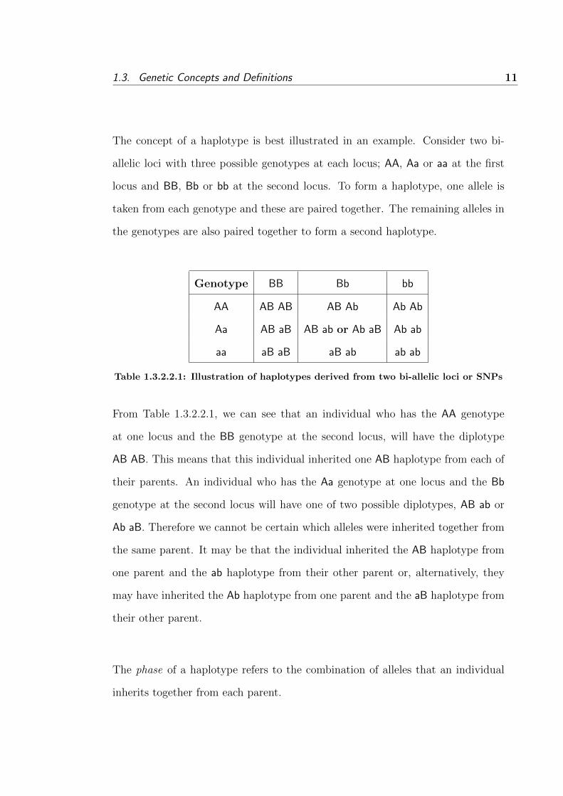
The concept of a haplotype is best illustrated in an example. Consider two bi-
allelic loci with three possible genotypes at each locus; AA, Aa or aa at the first
locus and BB, Bb or bb at the second locus. To form a haplotype, one allele is
taken from each genotype and these are paired together. The remaining alleles in
the genotypes are also paired together to form a second haplotype.
Genotype BB Bb bb
AA AB AB AB Ab Ab Ab
Aa AB aB AB ab or Ab aB Ab ab
aa aB aB aB ab ab ab
Table 1.3.2.2.1: Illustration of haplotypes derived from two bi-allelic loci or SNPs
From Table 1.3.2.2.1, we can see that an individual who has the AA genotype
at one locus and the BB genotype at the second locus, will have the diplotype
AB AB. This means that this individual inherited one AB haplotype from each of
their parents. An individual who has the Aa genotype at one locus and the Bb
genotype at the second locus will have one of two possible diplotypes, AB ab or
Ab aB. Therefore we cannot be certain which alleles were inherited together from
the same parent. It may be that the individual inherited the AB haplotype from
one parent and the ab haplotype from their other parent or, alternatively, they
may have inherited the Ab haplotype from one parent and the aB haplotype from
their other parent.
The phase of a haplotype refers to the combination of alleles that an individual
inherits together from each parent.

12 Chapter 1. Introduction
1.3.2.3 Haplotype inference
It is not always possible to infer haplotype phase unambiguously. Recalling from
Figure 1.3.2.2.1, if an individual is homozygous at one or both loci, then their
haplotype pair, or phase, can be constructed with certainty. However, if the in-
dividual is heterozygous at both loci, then their haplotype pair is referred to as
phase-ambiguous. This is because the individual inherited either the AB ab or the
Ab aB diplotype.
Several methods can be employed to construct these haplotypes with certainty,
including collecting data from family members or the use of laboratory techniques
to isolate the haplotypes to a particular chromosome, however these procedures
are often costly and time consuming [24]. As a consequence, several statistical
procedures have been developed in order to estimate the phase of diplotypes from
available genotypic information.
The three main statistical methods of haplotype inference are Clark’s Algorithm
[25], a pseudo-Bayesian algorithm by Stephens et al. [26], and an Expectation
Maximisation (EM) algorithm by Excoffier and Slatkin [24]. Clark’s Algorithm is
prone to several problems, for example, the algorithm cannot begin if there are
no individuals who are homozygous at all loci. The pseudo-Bayesian algorithm
also exhibits problems, particularly with the calculation of distributions. Niu et
al. [27] have shown that the conditional distributions calculated do not correspond
to a proper joint distribution; also the distributions calculated may depend on the
order of the genotypes [28]. The EM algorithm appears to exhibit less problems,
and is utilised by the statistical software package, SimHap, which is introduced in

1.3. Genetic Concepts and Definitions 13
Section 3.5.7 (please see page 214) and described further in Section 3.5.7.2 (please
see page 216).
1.3.3 Hardy-Weinberg equilibrium principle
The Hardy-Weinberg Equilibrium (HWE) principle is a fundamental concept in
population genetics, describing the distribution of genotypes in a population. The
basic idea of this principle is that allele and genotype frequencies remain constant
from one generation to the next, if the following conditions are met [29]:
1. The population is large enough so that sampling variation is negligible,
2. mating within the population occurs at random,
3. there is no selective advantage for any genotype; all genotypes are equally
viable and fertile, and
4. there is an absence of factors (‘evolutionary forces’) such as mutation, mi-
gration and random genetic drift.
Consider a locus consisting of two alleles, A and a, and let the frequencies of these
alleles be represented by p and q, respectively, where q=1-p. The HWE princi-
ple states that the genotype frequencies of AA, Aa and aa will be in proportions
p2, 2pq and q2, respectively. As long as the above four conditions are met, then
these genotype frequencies will remain constant generation after generation. De-
viations from HWE can be tested using Pearson’s Chi-Square or an exact test;
if the observed genotype frequencies are significantly different from the expected
frequencies then we would conclude the population is not in HWE. Evidence for

14 Chapter 1. Introduction
deviations from HWE may point to the violation of one of the above four as-
sumptions, or undetected genotyping errors; both of which could bias statistical
analyses [30].
1.3.4 Linkage disequilibrium
Linkage disequilibrium is a measure of the association between two alleles in a
population. Linkage disequilibrium occurs when some combinations of alleles on
the same chromosome (i.e. a haplotype) occur more often than would be ex-
pected by chance. Linkage disequilibrium results from ancestral recombination
events. Both linkage and linkage disequilibrium measure cosegregation, however
linkage measures cosegregation within families, while linkage disequilibrium mea-
sures cosegregation within the population.
To explain linkage disequilibrium further, define PA, Pa, PB and Pb to be the fre-
quencies of the A, a, B and b alleles respectively, and PAB to be the frequency of
the AB haplotype. When there is no evidence for disequilibrium, that is, when al-
leles are in equilibrium, there will be independence between the allele frequencies
at the two loci. This means that PA|B = PA, or the probability of an individual
having the A allele given they have the B allele, is just equal to the probability
of having the A allele. Also, at equilibrium, PAB = PAPB, or the probability of
having the AB haplotype, is the product of the probabilities of having both the A
allele and the B allele.
When linkage disequilibrium is present, the probability of observing the AB hap-
lotype is PAB = PAPB + D, where D is the linkage disequilibrium coefficient and
1.4. Gene Discovery in Human Disease 15
measures the strength of disequilibrium. As D is highly dependent on allele fre-
quencies, D can be standardised to D′ (referred to as Lewontin’s D′) [31], by
D′ = DDmax
, where Dmax is the largest possible value that D can take and is equal
to min(PAPb, PaPB). D′ will take a value between 0 and 1, with a larger value
indicating stronger linkage disequilibrium. If D′ equals zero, then there is random
association between different alleles at different loci and we have equilibrium. A
D′ of 1 occurs when the two loci are perfectly correlated, and any value of D′
above 0.8 is generally considered evidence for strong disequilibrium.
Another measure of linkage disequilibrium is the correlation coefficient between
two loci, r [4] and is defined by DPA−Pa−P−BP−b
, where PA− is the probability of
the AB or Ab genotype, Pa− is the probability of the aB or ab genotype, P−B is
the probability of the AB aB genotype, and P−b is the probability of the Ab or
ab genotype. Similar to the standard correlation coefficient, r may take a value
between -1 and 1.
Evidence for linkage disequilibrium can be helpful in discovering disease genes,
and this is described further in the following section.
1.4 Gene Discovery in Human Disease
The recent sequencing of the human genome has facilitated a dramatic acceleration
in human disease gene discovery. This section describes some analytic methods
used to investigate and identify the genetic causes of human disease.

16 Chapter 1. Introduction
1.4.1 Simple and complex disease
Human diseases are often categorised into two types - simple disease and com-
plex disease. The terms ‘simple’ and ‘complex’ refer to the genetic nature of the
disease. Simple diseases are caused by a mutation in a single gene, and are often
referred to as monogenic or Mendelian diseases. The variants that cause simple
diseases are rare, and generally have high penetrance. These diseases are inher-
ited based on a known pattern of inheritance, whereby disease clearly segregates
within families. Examples of simple genetic diseases are cystic fibrosis which has
a recessive pattern of inheritance [32], and Huntington’s disease which has a dom-
inant inheritance pattern [33].
Complex diseases are caused by variation in many genes, and by environmental
factors and interactions of these; and it is likely that each individual genetic locus
contributes only modestly to the disease. Complex diseases are generally common
in a population relative to monogenic diseases and include cardiovascular disease,
asthma and many cancers, including melanoma. Complex diseases do not follow
a known pattern of inheritance, and while these diseases are more common in
relatives of those with the disease, they do not segregate within families with a
clear pattern of inheritance.
Due to the differences between simple and complex diseases, namely, that simple
diseases are rare and tend to segregate within families, while complex diseases
commonly occur in the general population, different gene discovery methods are
required. Two of these methods, linkage analysis and genetic association studies,
are described in the following sections – Section 1.4.2 and 1.4.3.

1.4. Gene Discovery in Human Disease 17
1.4.2 Linkage analysis
Traditionally, the identification of simple disease genes has begun with family-
based linkage analysis, as linkage analysis uses pedigrees and can be used to locate
areas of the genome that contain disease genes. Linkage analysis exploits the con-
cept of linkage, which was introduced in Section 1.3.4. That is, loci that are close
together on a chromosome will be inherited together more often than expected by
chance, as they will have experienced lower recombination events than loci further
apart. In linkage analysis, genetic markers that are evenly distributed through
the genome are genotyped and their segregation through a pedigree is studied.
If family members with disease often have the same genetic markers, that is, if
disease cosegregates with the markers, then it is possible to infer the position of
the disease gene.
Linkage analysis has been very successful in identifying disease-gene regions for
simple diseases involving a single locus, such as Huntington’s disease. Simple dis-
ease variants are often rare and highly penetrant, and therefore the disease allele
can be localised to a small chromosomal region, and linkage markers close to the
disease allele will cosegregate with disease [34]. In contrast, linkage analysis has
had only limited success at identifying the genes that cause complex diseases [35].
This lack of success is due to a number of factors, including the low heritability of
complex disease, low resolution to localise disease alleles to a particular chromo-
somal location and inadequately powered studies due to the small effect of each
disease locus [34]. It has been shown that for linkage analysis to have enough
statistical power to detect a relative risk of 2, at least 2,500 families need to be
studied [36]. A relative risk of 2 is considered to be a large relative risk conferred

18 Chapter 1. Introduction
by a disease locus in a complex disease [37], therefore any linkage analysis with less
than 2,500 families would be unlikely to detect genetic causes of complex disease.
1.4.3 Genetic association studies
Genetic association studies are used to discover both genetic and environmental
risk factors for disease. In contrast to linkage studies that are primarily used for
family-based studies, association studies can be used for both family-based and
population-based studies. However, association studies have often been used in
conjunction with linkage analysis; that is, when a disease locus is localised to a
chromosomal region, association studies can be used to investigate the region in
order to locate the specific disease-causing allele [38]; this is referred to as fine
mapping.
There are two major types of genetic association studies - candidate-gene stud-
ies and genome-wide association studies (GWAS). Both types of studies exploit
the concept of linkage disequilibrium between alleles which was described earlier
in Section 1.4.2. In a candidate-gene study, genes suspected of being involved in
causing disease are identified using selection criteria, such as biological plausibility,
animal models, or prior associations [39]. Tests of associations between variants in
these genes and the disease outcome are then performed. More recently, genetic
association studies are being performed over the entire genome, and are referred
to as GWAS. This approach is often preferred over the candidate-gene study in
complex disease genetics, as no assumptions are made about the identity of the
causal gene.

1.4. Gene Discovery in Human Disease 19
In both types of studies, associations detected between genetic variants and dis-
ease outcomes may be due to one of three reasons. The first of these is direct
association, that is, the variant tested is functional and directly causes the out-
come. These associations tend to be the easiest and most powerful to analyse [40].
However, the prior probability that a given associated variant is itself functional
is generally low. More likely is that indirect association occurred; that is, the
variant associated with the outcome is in linkage disequilibrium with the causal
variant. The third possibility is that the association was spurious, although this
possibility can be fully or partially eliminated by applying appropriate statistical
tools, such as adjusting for multiple testing.
1.4.4 Multiple testing
In statistical analyses, the probability of a type I error or ‘false positive’ is the prob-
ability of rejecting the null hypothesis when it is actually true. When performing
one statistical test, this probability, or α, is referred to as the significance level and
is commonly set at 0.05. This means that when performing one test, the probabil-
ity that the result will be a false positive is 0.05, and so for the association to be
deemed significant, the observed p-value needs to be below this value. When per-
forming n multiple comparisons or tests simultaneously, the probability of a false
positive increases to 1− (1− α)n. Multiple testing issues are common in genetic
association studies due to the testing of multiple genetic markers simultaneously.
For example, when testing associations between 42 genetic variants or SNPs and
some outcome, the probability of at least 1 false positive is 1−(1−0.05)42=0.8840.
Traditionally, the Bonferroni correction has been used to adjust for multiple com-
parisons. In this correction, the total error rate of all tests combined is set at α,

20 Chapter 1. Introduction
so that each test has an individual type I error rate of αn. When testing 42 SNPs,
this would lead to an adjusted significance level of 0.0542
= 0.00119. Therefore,
associations with a p-value < 0.00119 would be deemed significant. The Bonfer-
roni correction is considered by some to be too conservative when the number of
genetic variants tested is high [41].
Genetic analyses in this thesis use the False Discovery Rate (FDR) method [42]
instead of the Bonferroni correction to adjust for multiple testing. The FDR
approach controls the expected proportion of false positives, compared to the
Bonferroni correction that controls the chance of any false positives assuming a
null hypothesis at any genetic loci.
The FDR approach can be used to estimate an FDR threshold known as q. The
q value is calculated as q(r) =m∗p(r)r
, where m is the number of SNPs tested and
p(r) is the p-value of the rth SNP when the SNP p-values are ordered from lowest
to highest. In this thesis, this value of q was compared to α, and the test was
deemed significant when q < α, where α was defined at the 5% significance level.
The FDR approach was used to calculate the q threshold for each SNP at the
multivariate genotypic analysis stage.
1.5 Aims
This thesis investigates the genetic epidemiology of melanoma susceptibility and
prognosis in the Western Australian Melanoma Health Study (WAMHS). In ad-
dition, this thesis describes a technique known as Mendelian randomisation, and
an application of this technique for making causal inferences in epidemiological

1.6. Outline of thesis 21
studies.
The aims in this thesis are described below:
1. To assist in establishing the WAMHS,
2. to investigate associations between candidate loci and melanoma risk in the
WAMHS sample,
3. to investigate associations between known host, environmental and genetic
melanoma-risk factors with melanoma prognosis, as reflected by Breslow
thickness, in the WAMHS sample, and
4. to implement a statistical technique known as Mendelian randomisation in
R, and to undertake novel methods development to enable the use of both
SNP and haplotypes to model causality in epidemiological studies.
1.6 Outline of thesis
Chapter 2 of this thesis begins with a description of melanoma incidence and mor-
tality rates and follows with a comprehensive review of the genetic epidemiology
of melanoma susceptibility and prognosis. The WAMHS is described, and in the
following sections, these data are used to investigate the role of genetic variants
in melanoma susceptibility. WAMHS data are also used to test the hypothesis
that the genetic, environmental and host factors that increase melanoma risk are
also associated with Breslow thickness, which is the main prognostic feature of
melanoma. This chapter finishes with a summary of the key findings and their
implications in melanoma research.

22 Chapter 1. Introduction
In Chapter 3, a background to epidemiological studies, in particular observational
epidemiological studies, is presented. I then described a statistical method known
as Mendelian randomisation that can be used to detect causal associations between
disease outcomes and modifiable exposures in epidemiological association studies.
The implementation of this method in an R library, MRsnphap, is also described,
along with novel methods work to extend Mendelian randomisation to haplotypes.
Chapter 4 summarises the main results of this thesis and describes areas for further
research, including possible further development of MRsnphap.

23CHAPTER 2
Genetic Epidemiology of Malignant Melanoma:
Susceptibility and Prognosis in the WAMHS
This chapter begins with a description of the incidence and mortality of melanoma
in recent years, followed by a review of the genetic, host and environmental risk
factors for melanoma development and prognosis. Establishment of the WAMHS
is then described. Following this, I took known candidate variants for melanoma
risk and tested whether these genetic variants were associated with melanoma in
a sub-sample of the WAMHS. I also used the WAMHS data to investigate the role
of melanoma-risk factors in melanoma prognosis. The results of these analyses
are then presented and discussed.
2.1 Introduction
Melanoma is a significant public health issue in Australia and worldwide. Aus-
tralia has the highest incidence rate of melanoma in the world, with over 10,000
cases diagnosed each year [43]. Melanoma was first described as a disease by Rene
Laennec in 1804 [44], however the first recorded operation on metastatic melanoma
was performed some years earlier in 1787 by John Hunter [45]. As early as 1840,
the British surgeon Samuel Cooper recognised that ‘the only chance for benefit de-
pends upon early removal of disease’ [46]; to date, early excision of the melanoma
tumour is the standard treatment, and is the only potentially curative treatment
for melanoma [47].
Melanoma is a complex disease resulting from mutations in many genes, environ-
mental and host factors and their interactions. In 1956, John Lancaster observed
a geographical distribution of melanoma mortality which supported the role of

24Chapter 2. Genetic Epidemiology of Malignant Melanoma: Susceptibility and
Prognosis in the WAMHS
sun exposure in causing melanoma [48]. Sun exposure is still considered to be the
main environmental risk factor for melanoma, however its interactions with other
environmental, host and genetic factors and their role in melanoma development
and prognosis are less clearly understood. To date, several genes for melanoma
have been identified, however mutations in these genes are rare and only account
for a small proportion of melanoma diagnoses [49]. Population-based studies of
melanoma cases may help to elucidate the role of environmental, host and genetic
risk factors of melanoma development and prognosis.
2.2 Literature Review
2.2.1 Skin cancer
It is estimated that 2 in 3 Australians will be diagnosed with skin cancer be-
fore the age of 70 [50]. Cutaneous Malignant Melanoma (hereafter referred to as
melanoma), Basal Cell Carcinoma (BCC) and Squamous Cell Carcinoma (SCC)
are the three main types of skin cancers and accounted for approximately 82% of
all cancer diagnoses in Australia in 2002 [50]. Together, the non-melanoma skin
cancers, including mostly BCC and SCC, accounted for approximately 67% and
30% of Australian skin cancer diagnoses, respectively [51]. Melanoma is the rarest
form of these skin cancers and accounted for approximately 3% of Australian skin
cancer diagnoses [51].
While BCC and SCC are the most common types of skin cancer, mortality rates
from these cancers are much lower than those of melanoma. In 2005, approxi-
mately 3.1 per 100,000 males and 1 per 100,000 females died from non-melanoma
skin cancers [52]. In contrast, mortality rates from melanoma were approximately

2.2. Literature Review 25
three-fold those of the non-melanoma skin cancers, at 8.9 per 100,000 males
and 3.5 per 100,000 females [51]. In real terms, 411 Australians died from non-
melanoma skin cancers in 2005, while 1,262 Australians died from melanoma. As
such, it is important from a clinical and public health viewpoint that the mecha-
nisms underlying melanoma, in particular melanoma susceptibility and prognosis,
are more clearly understood.
2.2.2 Melanoma biology
Melanoma is a complex and aggressive form of cancer of the melanocytes. In the
skin, melanocytes are cells found in the deepest layer of the epidermis (See Figure
2.2.2.1). When exposed to sunlight, melanocytes produce and supply melanin to
protect the keratinocytes from mutation due to ultraviolet radiation. Melanin is
the pigment found in the skin, hair and eyes and once produced, is responsible for
tanning.
The Clark model [53,54] has been used to describe the progression of melanoma in
five stages, from normal melanocytes to development of metastatic melanoma. It is
estimated that up to 70% of melanomas may arise de novo from normal-appearing
skin, although this is difficult to determine [55–57]. Therefore, the development of
melanoma may begin in either stage 1 or stage 2 of the Clark’s model. In addition,
not all melanoma tumours experience radial or vertical growth [53]. As such, the
Clark model should be viewed as a general framework for melanoma growth, with
not all tumours progressing through all stages. The stages of Clark’s model are
shown in Figure 2.2.2.2.

26Chapter 2. Genetic Epidemiology of Malignant Melanoma: Susceptibility and
Prognosis in the WAMHS
Figure 2.2.2.1: Cross-section of the skin highlighting the epidermal layer
The five stages of the Clark model are described below:
1. Benign naevus – structurally normal melanocytes proliferate to form be-
nign naevus. These naevi may be flat or slightly raised lesions, are generally
a tan or dark brown colour, and rarely develop into melanoma.
2. Dysplastic naevus – aberrant growth begins in either a pre-existing be-
nign naevus, or in a new location. These lesions may be varying colours,
asymmetrical, or have irregular borders, and are generally 5mm or greater
in diameter.
3. Radial growth - cells acquire the ability to grow into the epidermis. If the
melanoma is removed before cells have spread outside of the epidermis, the

2.2. Literature Review 27
Figure 2.2.2.2: Clark model of the five stages of melanoma development, from
normal melanocytes to metastatic melanoma [54]
melanoma is referred to as in situ melanoma.
4. Vertical growth - lesions acquire the ability to grow into a deeper layer of
the skin, the dermis, and may also grow into the subcutis. These melanomas
are referred to as invasive melanomas, and are the focus of this thesis.
5. Metastatic melanoma - cancerous cells spread to other areas of the skin
and internal organs through the lymphatic system and via the blood stream,
where they can proliferate.
2.2.3 Melanoma incidence and mortality
2.2.3.1 Melanoma in Australia
Australia has the highest incidence of melanoma in the world [43] and this is ris-
ing [51]. Melanoma incidence rates in Australia are more than double those in

28Chapter 2. Genetic Epidemiology of Malignant Melanoma: Susceptibility and
Prognosis in the WAMHS
the United States of America, and about four times those in the United Kingdom
and Canada. Incidence rates for these countries and selected others are shown
in Figure 2.2.3.1.1. The age-standardised rates presented in Figure 2.2.3.1.1 are
based on the 2001 World Standard Population. To allow for comparisons between
Australian and Western Australian incidence and mortality rates, all rates here-
after are based on the 2001 Australian Standard Population.
Melanoma incidence rates in Australia and New Zealand are significantly higher
compared to other countries in the world. This may be due to a number of rea-
sons, including environmental, geographic, and cultural reasons. For example,
ultraviolet exposure is a known risk factor for melanoma [65], and ultraviolet ex-
posure levels are higher at lower latitudes. In addition, many Australians and
New Zealanders tend to have fair skin due to European ancestry, and therefore
their skin is naturally more suited to areas of low ultraviolet exposure. However,
even with skin poorly suited to the high levels of ultraviolet exposure in Australia
and New Zealand, many Australians and New Zealanders participate in outdoor
recreational activities throughout the year from childhood to adulthood, which
increases ultraviolet exposure and therefore melanoma incidence.
An estimated 10,684 new cases of melanoma were diagnosed in Australia in 2005.
Melanoma was the third most diagnosed cancer (excluding SCC and BCC) in
2005 in both Australian males and females, after prostate and colorectal can-
cer in males, and breast and colorectal cancer in females. Melanoma accounted
for approximately 10% of cancer diagnoses [51]. Males are approximately 1.5
times more likely to be diagnosed with melanoma compared to females, with 2005
age-standardised incidence rates of 60.9 per 100,000 males and 42.5 per 100,000

2.2. Literature Review 29
Figure 2.2.3.1.1: Melanoma incidence rates for selected countries for males and
females. Incidence rates are presented as age-standardised rates (per 100,000 per-
sons) based on the 2001 World Standard Population. Data obtained from Globocan
2002 [43].
females [51]. While the incidence of melanoma is significantly higher in males
compared to females in Australia, New Zealand, and the United States of Amer-
ica, female incidence tends to be higher than male incidence in European countries
(2.2.3.1.1). The reasons for this remain unclear.
Melanoma incidence has been increasing steadily since 1982 (see Figure 2.2.3.1.2),
with 2005 age-standardised rates approximately double those in 1982. Currently,
it is predicted that 1 in 26 Australians will develop melanoma before the age of
75 [51], however this risk was 1 in 35 in 1990 [58], and 1 in 49 in 1982 [59]. It

30Chapter 2. Genetic Epidemiology of Malignant Melanoma: Susceptibility and
Prognosis in the WAMHS
is predicted that incidence rates will continue to rise in Australia at least until
2011 [51]. It is evident from Figure 2.2.3.1.2 that in the early 1980s, incidence in
males and females was comparable, and it was only in 1985 that male incidence
increased in comparison to female incidence. As this disparity in male and female
melanoma incidence occurred only recently, it is not likely that the higher inci-
dence in males is driven by underlying biological differences between the sexes,
but may be due to an increase in ultraviolet exposure in males.
Figure 2.2.3.1.2: Melanoma incidence rates from 1982 to 2005 for males and females.
Incidence rates are presented as age-standardised rates (per 100,000 persons) based
on the 2001 Standard Australian Population. Data obtained from the Australian
Institute of Health and Welfare COGNOS data cube [60].
Melanoma is a cancer that affects both young and middle-aged individuals, unlike
most other cancers which tend to affect mainly older adults. In 2005, melanoma
was the most common cancer diagnosed in males aged between 16 and 51, and
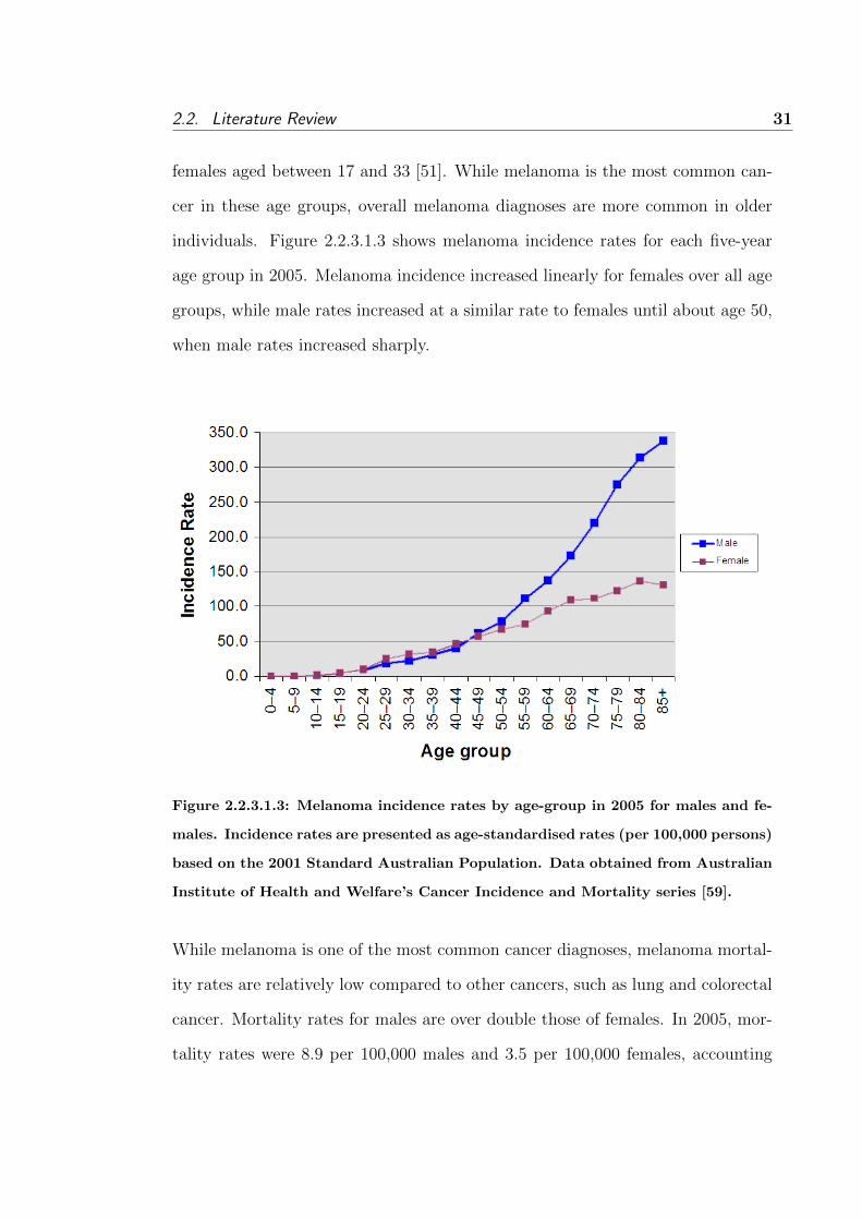
2.2. Literature Review 31
females aged between 17 and 33 [51]. While melanoma is the most common can-
cer in these age groups, overall melanoma diagnoses are more common in older
individuals. Figure 2.2.3.1.3 shows melanoma incidence rates for each five-year
age group in 2005. Melanoma incidence increased linearly for females over all age
groups, while male rates increased at a similar rate to females until about age 50,
when male rates increased sharply.
Figure 2.2.3.1.3: Melanoma incidence rates by age-group in 2005 for males and fe-
males. Incidence rates are presented as age-standardised rates (per 100,000 persons)
based on the 2001 Standard Australian Population. Data obtained from Australian
Institute of Health and Welfare’s Cancer Incidence and Mortality series [59].
While melanoma is one of the most common cancer diagnoses, melanoma mortal-
ity rates are relatively low compared to other cancers, such as lung and colorectal
cancer. Mortality rates for males are over double those of females. In 2005, mor-
tality rates were 8.9 per 100,000 males and 3.5 per 100,000 females, accounting

32Chapter 2. Genetic Epidemiology of Malignant Melanoma: Susceptibility and
Prognosis in the WAMHS
for 3.9% and 2.4% of cancer deaths in males and females respectively [51].
The higher mortality rates in males may be due to the different characteristics of
male melanomas compared to female melanomas. For example, males are more
likely to have thicker melanomas excised, have melanomas excised from different
body sites, and have ulceration of the melanoma [271]. However, several studies
have found that even after adjustment for these factors, male sex remains an in-
dependent predictor for prognosis [270, 271], indicating that there may be other
sex-specific factors that affect mortality rates.
Figure 2.2.3.1.4 shows melanoma mortality rates from 1968 to 2005. Melanoma
mortality rates for females remained relatively stable from 1968 to 2005; however
male mortality rates have increased approximately two-fold since 1968. Melanoma
mortality rates are predicted to continue to rise slightly in males, while female
rates are predicted to remain stable [51]. The different trends in mortality be-
tween males and females is substantial, however few studies have been published
which attempt to explain this difference.
Although Australia has a much higher incidence rate than other countries, the
differences in melanoma mortality between Australia and other countries are not
as extreme. For example, the age-standardised incidence rate for melanoma in
the United Kingdom (UK) is approximately one–quarter of Australian melanoma
incidence, while the mortality rate of UK individuals with melanoma is less than
one–third of Australian mortality (8.9 in Australian males and 3.5 in Australian
females compared to 3.0 in UK males and 2.0 in UK females) [273]. This sug-

2.2. Literature Review 33
gests that while Australians are more likely to be diagnosed with melanoma, early
detection and improved treatment of melanoma results in proportionally less Aus-
tralians dying from the disease.
Figure 2.2.3.1.4: Melanoma mortality rates from 1968 to 2005 for males and females.
Mortality rates are presented as age-standardised rates (per 100,000 persons) based
on the 2001 Standard Australian Population. Data obtained from Australian Insti-
tute of Health and Welfare’s Cancer Incidence and Mortality series [59]
Australia-wide, five-year survival rates in both males and females increased over
the 22 year period from 1982 to 2004. Between 1982 and 1986, five-year survival
rates in males were 82.2%, increasing to 89.7% between 1998 and 2004. Similarly
for females, five-year survival rates increased from 90.5% between 1982 and 1986
to 94.1% between 1998 and 2004 [61]. These increases in survival may be partly
due to the earlier detection of melanoma (i.e. thinner melanomas with better

34Chapter 2. Genetic Epidemiology of Malignant Melanoma: Susceptibility and
Prognosis in the WAMHS
prognosis excised), and also advances in treatment.
2.2.3.2 Melanoma in Western Australia
Western Australia has the second-highest melanoma incidence in Australia, after
Queensland [51]. Average incidence rates of all Australian states and territories
from 2001 to 2005 can be seen in Figure 2.2.3.2.1.
Figure 2.2.3.2.1: Melanoma incidence rates for all Australian states and territories
from 2001 to 2005 for males and females. Incidence rates are presented as age-
standardised rates (per 100,000 persons) based on the 2001 Standard Australian
population. Data obtained from Australian Institute of Health and Welfare’s Can-
cer Report [51].
At the time of writing this thesis, 2007 melanoma incidence and mortality rates
in Western Australia were available; however due to an issue with data collec-
tion at the Western Australian Cancer Registry, the 2007 rates are believed to be

2.2. Literature Review 35
understated (further details are available in the 2007 Western Australian Cancer
Incidence and Mortality report [62]). Therefore, only melanoma rates for 2005
and 2006 will be discussed in this section.
In 2005, melanoma diagnoses accounted for 11% of cancer diagnoses in Western
Australian males and 9.8% in Western Australian females, which made melanoma
the 4th and 3rd ranked cancer in males and females respectively (after prostate,
lung and colorectal cancer in males, and breast and colorectal cancer in females)
[63]. In 2006, melanoma diagnoses accounted for slightly more of the cancer diag-
noses (11.1% for males and 10.6% for females), with melanoma the 2nd and 3rd
ranked cancer for males and females respectively (after prostate cancer in males,
and breast and colorectal cancer in females) [64].
Of the 10,684 melanomas diagnosed in Australia in 2005, approximately 9% were
in Western Australians [63]. This corresponded to incidence rates of 59.3 cases
per 100,000 males and 37.8 cases per 100,000 females [63]. Incidence rates in both
males and females increased in 2006 to 60.9 cases per 100,000 males and 42.5 cases
per 100,000 females [63].
In Western Australia, the 2005 mortality rates were 11.6 deaths per 100,000 males
and 3.2 deaths per 100,000 females [63]; mortality rates in females were compa-
rable to the 2005 Australian mortality rates, however male mortality rates were
significantly higher in Western Australian males. In 2006, Western Australian
mortality rates in males decreased to 9 deaths per 100,000, while mortality rates
in females increased to 4.3 deaths per 100,000 [64]. There is no obvious reason for

36Chapter 2. Genetic Epidemiology of Malignant Melanoma: Susceptibility and
Prognosis in the WAMHS
2005 mortality rates to be higher in Western Australian males compared to other
Australian males. This may have been a chance fluctuation in rates in 2005, as
in 2006 male mortality rates were consistent with the national average.
2.2.4 The aetiology of malignant melanoma
Melanoma is a cancer that results from complex interactions between genetic,
host and environmental factors. Epidemiological research in melanoma has led to
some understanding of the host factors which increase an individual’s melanoma
risk; these include pale complexion, red or blonde hair, skin that freckles easily
and tans poorly, many naevi (or moles), and a family history of melanoma [65].
The strongest risk factor for melanoma is a large number of naevi [66], while
the main established environmental risk factor for melanoma is sun exposure, in
particular exposure to ultraviolet radiation (UVA and UVB) [65]. Several genes
which may predispose an individual to melanoma have been identified. Like any
complex disease, however, it is thought that a combination of the genetic, host
and environmental factors contribute to the development of melanoma.
2.2.4.1 Environmental and host melanoma risk factors
2.2.4.1.1 Sun exposure
Sun exposure is the principle established environmental risk factor for melanoma
and this was recognised by the International Agency for Cancer Research in
1992 [67]. Sun exposure history can be measured by either migrant studies or
personal exposure studies; however sun exposure is notoriously difficult to mea-
sure. Personal exposure case-control studies that ask individuals to recall their

2.2. Literature Review 37
sun exposure are often subject to recall and other biases [68,69]. In these studies,
a proxy measure of sun exposure is often used (for example, sunburn history)
and individuals must rely on recollection, sometimes from sun exposures experi-
enced decades earlier. However, these observational studies are often performed,
as RCTs are not considered ethical, and longitudinal cohort studies can be costly
and time-consuming. Migrant studies, also known as ambient studies, have an
advantage over personal exposure studies, as migration from areas of low/high in-
solation to areas of high/low insolation tend to be easy to classify and record [70].
Cumulative sun exposure throughout a whole lifetime has been established as a
risk factor for melanoma; however it has been hypothesised that childhood sun ex-
posure may confer a higher melanoma risk than similar exposure in later life [70].
This has been investigated in both migrant studies [71–82] and personal exposure
studies [83].
In a meta-analysis by Gandini et al. [83] of 33 personal exposure studies, sunburn
was associated with an increased risk of melanoma, with an overall relative risk
of 2.03 (95% CI = 1.73, 2.37). When further stratified by age, childhood sunburn
(less than 15 years of age) conferred a relative risk of 2.24 (95% CI = 1.73, 2.89),
while adulthood sunburn (greater than 19 years of age) conferred a relative risk
of 1.92 (95% CI = 1.55, 2.37). However, the meta-analyses was not adjusted for
skin type or the ability to tan which are likely to affect both incidence of sunburn
and melanoma.
Migrant studies are often used to investigate the relationship between sun expo-

38Chapter 2. Genetic Epidemiology of Malignant Melanoma: Susceptibility and
Prognosis in the WAMHS
sure in childhood and melanoma risk. A comprehensive review by Whiteman et
al. [70] of migration studies and melanoma risk investigated place of birth and
age at migration. In 11 of the 12 place of birth studies, individuals born in ar-
eas of low insolation (e.g. United Kingdom) who later migrated to areas of high
insolation (e.g. Australia) had lower risks of developing melanoma than natives
of these high insolation areas [71–81]. Only one study showed the opposite effect,
with migrants to Hawaii having an increased risk of melanoma [82]. The results
from these 11 studies suggest that individuals who migrate to areas of high in-
solation from areas of low insolation have, in general, lower melanoma incidence
than native-born and raised individuals. This indicates that living in areas of low
insolation for the earlier years of life may protect against melanoma compared to
living in high insolation areas for a lifetime. These studies, however, do not take
age at migration into account which may also play a significant role.
Of the five comparable studies examining age at migration from low insolation to
high insolation areas [74,75,79,84,85], three studies found that a decreased risk of
mortality from melanoma was associated with older age at migration [74, 75, 84].
In particular, a study by Khlat et al. [74] comparing mortality rates of migrants
to native-born individuals, found that when migration to Australia occurred be-
tween the ages of 15 and 24, male melanoma mortality dropped to 0.41 (95% CI
= 0.32, 0.54), and migration after the age of 25 was associated with an even lower
risk of mortality, 0.32 (95% CI = 0.27, 0.39).
Similarly, in a study by Darcy et al. [84] melanoma incidence was lower in in-
dividuals who migrated at a later age. In particular, melanoma incidence was
reduced significantly at migration after 19 years of age, with a risk ratio of 0.25

2.2. Literature Review 39
(95% CI = 0.08, 0.83), when compared to migration before 19 years of age. These
studies suggest that melanoma incidence and mortality are both affected by age
at migration. More specifically, migration in childhood increases melanoma risk
to closer to that of a native-born individual and migration before the age of 15
increases melanoma mortality.
There is continuing debate over what type of sun exposure confers the highest
melanoma risk. It has been suggested that intermittent exposure, which can be
categorised as either recreational or vacation exposure [86], confers a higher risk
of melanoma than occupational or chronic sun exposure. In a 2008 meta-analysis
by Gandini et al. [83] of 33 case-control studies, intermittent sun exposure was
associated with melanoma with a relative risk of 1.61 (95% CI = 1.31, 1.91), while
occupational sun exposure was not significantly associated with melanoma with a
relative risk of 0.95 (95% CI = 0.87, 1.04). These results suggest that intermittent
sun exposure may increase the risk of melanoma, while occupational sun exposure
either reduces or has no effect on melanoma risk.
2.2.4.1.2 Skin type and pigmentation
Pigmentation, including skin, hair and eye colour, plays an important role in
melanoma development. In particular, fair-skinned individuals are more likely to
develop melanoma than darker-skinned individuals [87], with melanoma risk in-
versely correlated to degree of pigmentation [88]. In fact, dark-skinned individuals
are unlikely to develop melanoma, with the majority of all melanomas diagnosed
in Caucasians. In a recent report of melanoma risk in an Australian Indigenous
population, the melanoma rate in the Indigenous population was 3.4 cases per
100,000, compared to 48.2 cases per 100,000 in the Australian non-Indigenous

40Chapter 2. Genetic Epidemiology of Malignant Melanoma: Susceptibility and
Prognosis in the WAMHS
population [62]. Bliss et al., [89] reviewed seven studies investigating the associa-
tion between melanoma and skin colour. When compared to dark skin, light skin
colour was associated with an approximate two-fold increased risk of melanoma,
mostly unaltered by naevus count, hair colour and freckling.
Melanoma risk is also independently associated with other pigmentation features,
including light hair colour, blue eyes and the presence of freckles [90,91]. A meta-
analysis of eight case-control studies [89] found that when compared to dark brown
hair, light brown, blonde and red hair conferred melanoma relative risks of 1.49
(95% CI = 1.31, 1.70), 1.84 (95% CI = 1.54, 2.21) and 2.38 (95% CI = 1.90,
2.97), respectively. These associations were observed independently of freckling
and skin colour. This meta-analysis also showed that when compared to brown
eyes, blue eyes conferred relative risks of 1.55 (95% CI = 1.35, 1.75), however this
association was not significant after adjustment for freckling [89]. Additionally,
in this meta-analysis, the presence of freckling when compared to sparse or no
freckling, was associated with a melanoma relative risk of 2.25 (95% CI=2.00,
2.54) and this association remained unchanged when adjusted for the presence of
naevi, skin and hair colour.
However, other researchers have cast doubt on the assertion that it is fair skin
that increases an individual’s melanoma risk, but instead suggest the tendency
to burn rather than tan following sun exposure is a better predictor of melanoma
risk [90,92]. A Western Australian study found that when compared to having a
deep tan, individuals with a moderate, light or no tan, had increased melanoma
relative risks of 1.4 (95% CI = 1.1, 1.9), 2.3 (95% CI = 1.6, 3.3) and 3.5 (95% CI
= 1.8, 6.8), respectively [87]. This association appeared to be explained by skin

2.2. Literature Review 41
and eye colour, but not hair colour. Similarly, a case-control study of American
adults found that individuals who had a deep tan had a reduced risk of melanoma
with an odds ratio of 0.47 (95% CI = 0.34, 0.65) for males and 0.43 (95% CI =
0.28, 0.65) for females, when compared to those with no tan [92].
While the relationship between pigmentation and melanoma development is com-
plex, fair-skinned individuals with light hair, blue eyes, freckles and who are un-
able to develop a deep tan, generally appear to be at a greater risk of developing
melanoma.
2.2.4.1.3 Family history
Melanoma clearly aggregates within families. It has been estimated that 10% of
individuals with melanoma have a first- or second-degree relative with melanoma
[93]. Early studies estimated that family history of melanoma caused a two- to
eight-fold relative risk for melanoma development [91,94]. However, a more recent
meta-analysis of 14 studies estimated a family history of melanoma (having one
or more affected first-degree relatives) confers a relative risk of only 1.74 (95% CI
= 1.41, 2.14) [95].
This aggregation of melanoma within families could possibly be due to shared host
factors such as eye colour, hair colour and naevus counts and also shared envi-
ronmental exposures found within families. However, Ford et al. [96] pooled eight
studies and found that, independent of these host factors, first-degree relatives of
individuals with melanoma had an estimated relative risk of 2.24 (95% CI = 1.76,
2.86). It has also been proposed that relatives of individuals with melanoma tend

42Chapter 2. Genetic Epidemiology of Malignant Melanoma: Susceptibility and
Prognosis in the WAMHS
to have an earlier age at onset, have thinner melanomas and are more likely to
develop multiple melanomas [94,97].
2.2.4.1.4 Naevi
The presence of multiple naevi is the main risk factor for melanoma. Most epi-
demiological studies that have investigated naevi and melanoma risk have found
that the presence of naevi are an independent risk factor for melanoma, particu-
larly the presence of atypical naevi [98]. The link between melanoma and naevi
was discovered in melanoma families who often have the Atypical Mole Syndrome
(AMS) phenotype. AMS is characterised by the presence of many common and
atypical naevi, typically over 100, which tend to appear in abnormal areas of the
body [99]. The AMS phenotype has been shown to be associated with melanoma
with an odds ratio of 10.4 (95% CI = 5.0, 21.5) [100]. Additionally, the same study
found that individuals under 40 years of age with melanoma were more than twice
as likely to have the AMS phenotype (odds ratio of 16.1; 95% CI = 4.6, 57.5),
compared to individuals aged over 40 (odds ratio of 6.9; 95% CI = 2.9, 16.6). This
highlights the importance of age in relation to the AMS phenotype and melanoma.
Children in Australia with increased numbers of naevi were found to have more
sun exposure than those with fewer naevi [101]. As sun exposure is a known risk
factor for melanoma, it follows that naevi may also be associated with melanoma,
although this relationship may not be causal. A case-control study of Australian
adolescents with melanoma found that the presence of 100 or more naevi was
strongly associated with melanoma risk, with an odds ratio of 46.5 (95% CI =
11.4, 190.8), independent of sun exposure levels [102]. Therefore, it appears the
presence of naevi, particularly in individuals younger than 40, plays an important

2.2. Literature Review 43
role in the development of melanoma.
2.2.4.2 Melanoma genetic risk factors
Historically, genetic studies of families selected on the basis of multiple cases of
melanoma have been used to discover melanoma-susceptibility genetic variants
[103, 104]. These studies have been successful in identifying two high-penetrance
genes for melanoma - Cyclin-dependent kinase inhibitor 2A (CDKN2A) and Cyclin-
dependent kinase 4 (CDK4). More recently, population- and family-based GWAS
have successfully identified several melanoma-susceptibility loci [105–108]. In
addition, candidate gene studies and GWAS of unrelated individuals have suc-
cessfully identified low-penetrance common genes which modify melanoma risk
through known risk factors, including skin pigmentation and naevi count [105,109].
2.2.4.2.1 High penetrance melanoma-susceptibility genes
Two high-penetrance melanoma-susceptibility genes have so far been identified
– CDKN2A and CDK4. In 1994, germline mutations in CDKN2A (located on
chromosome 9p21) were discovered in families with a history of melanoma [103,
110]. CDKN2A encodes for two tumour suppressor proteins, p16(INK4a) and
p14(ARF), which have been shown to have a role in cell cycle regulation and senes-
cence. The p16 and p14 mutations have been found to be strongly associated with
familial melanoma, and it has been estimated that 20-55% of melanoma families
have these mutations [111]. While relatively common in melanoma-prone fami-
lies, CDKN2A mutations are rare in melanoma cases in the general population. A
large international population-based study by Berwick et al. [112] found CDKN2A
mutations in 3% of individuals diagnosed with more than one melanoma, and mu-

44Chapter 2. Genetic Epidemiology of Malignant Melanoma: Susceptibility and
Prognosis in the WAMHS
tations in 1.2% of individuals with only one diagnosed melanoma.
Estimation of the likelihood of developing melanoma among CDKN2A muta-
tion carriers varies depending on ascertainment. Bishop et al. [113] estimated
melanoma penetrance in individuals with CDKN2A mutations who had a fam-
ily history of melanoma to be 0.3 by age 50, and 0.67 by age 80. In contrast,
a population-based study by Begg et al. [114] which ignored family history of
melanoma, estimated penetrance to be 0.14 by age 50, and 0.28 by age 80. There-
fore, from these studies it appears that CDKN2A mutation carriers in the general
population have a much lower risk of developing melanoma compared to carriers in
melanoma families. However, these differences may also be due to ascertainment
bias, as individuals with a strong family history of melanoma may have been more
likely to participate in the study by Bishop et al. It is clear, however, that the
combination of the rarity of CDKN2A mutations and their low penetrance in the
general population suggests that CDKN2A does not account for many melanoma
diagnoses. In fact, in a population-based study of melanoma cases in Queensland,
Aitken et al. [115] estimated that only 0.2% of melanomas in Queensland were
due to mutations in CDKN2A.
Germline mutations in CDK4 - an oncogene located on chromosome 12q13 - were
identified in melanoma families by Zuo et al. [104] in 1996. Mutations in CDK4
have only been found in several families to date [104, 116], thus accounting for
only a small proportion of familial melanoma. CDK4 interacts with CDKN2A
and as such, clinical phenotypes including age at onset of melanoma and the
number of melanomas, are similar between melanomas cases in CDKN2A and
CDK4 mutation carrier families [117]. Among two CDK4 families, Goldstein et

2.2. Literature Review 45
al. [118] assessed the penetrance of CDK4 mutation carriers to be 0.63 (95% CI
= 0.42, 0.85).
2.2.4.2.2 Low penetrance melanoma-susceptibility genes
The first low-penetrance melanoma-susceptibility gene identified was the melanocortin
1 receptor (MC1R) gene, located on the 16q24.3 chromosome. Variants in this
gene have been associated with red hair, fair skin and freckling [119–121]. As
these are well-established melanoma risk factors, it is not surprising that variants
in MC1R are also associated with melanoma risk. Valverde et al. [122] found
MC1R mutation carriers had an increased relative risk of melanoma of 3.9 (95%
CI = 1.48, 10.35). In a subsequent study, Palmer et al. [121] found the three
major red hair colour variants each conferred an odds ratio of melanoma of 2.2
(95% CI = 1.6, 3.0), while having two of these variants conferred an odds ratio
of approximately double this at 4.1 (95% CI = 2.1, 7.9). When adjusted for hair
colour and skin type, the association between one variant allele and melanoma
risk became non-significant for individuals with fair skin, however this association
remained significant for individuals with medium skin type (odds ratio of 2.2;
95% CI = 1.2, 4.1) and olive or dark skin type (odds ratio of 10.8; 95% CI = 1.2,
4.1). Thus, it appears that MC1R plays an independent role in melanoma risk,
independent of the association with skin pigmentation.
A recent meta-analysis of MC1R variants and melanoma risk and pigmentation
phenotypes by Raimondi et al. [123] found seven of the nine most commonly
investigated putative candidate risk variants were significantly associated with
melanoma. Additionally, two of these variants were associated with red hair and
fair skin, while three variants were associated with red hair only. More recently,

46Chapter 2. Genetic Epidemiology of Malignant Melanoma: Susceptibility and
Prognosis in the WAMHS
in a GWAS undertaken by Bishop et al. [106], the rs258322 SNP near the MC1R
locus was strongly associated with melanoma (combined GWAS and replication P
= 1.97 x 10⁻⁶). This SNP was previously identified in a GWAS by Han et al. [124]
as a hair colour and skin pigmentation locus, although Han et al. suggested that
the signal from this SNP was explained by three already identified MC1R variants.
This indicates that the rs258322 SNP may not be an independent risk SNP for
pigmentation.
While MC1R variants have been proven to be low-penetrance melanoma loci
[121,122,125], MC1R variants are also associated with increased CDKN2A pene-
trance and lower age of melanoma diagnosis [126]. In an Australian study of 15
melanoma-families, Box et al. [126] found CDKN2A penetrance to be 0.5, with a
mean age of diagnosis of 58.1. In the presence of MC1R variants, this penetrance
increased to 0.84 with a lower mean age of diagnosis of 37.8. Additionally, Gold-
stein et al. [127] suggested that in individuals with CDKN2A mutations, multiple
MC1R variants may be associated with the development of multiple melanomas.
Therefore, MC1R appears to not only be a melanoma risk gene, but it may also
interact with CDKN2A, increasing melanoma risk and number of melanomas, and
reducing the age at diagnosis.
Epidermal Growth Factor (EGF) located on chromosome 4q25-q27 has been im-
plicated as a melanoma-susceptibility gene. Shahbazi et al. [128] found a signif-
icant association between the rs4444903 SNP in EGF and melanoma risk, with
homozygous carriers of the rare allele having an increased odds of melanoma of
4.9 (95% CI = 2.3, 10.2). However, subsequent studies failed to detect any such
associations [129–132]. Some of these studies did detect significant associations
2.2. Literature Review 47
between the EGF variant and melanoma progression and this is discussed further
in Section 2.2.6 (please see page 50).
The recent advent of GWAS technology has enabled melanoma researchers to take
an unbiased approach in identifying melanoma-risk genes. To date, a number of
GWAS for melanoma risk, naevi count and pigmentation have been conducted.
A GWAS of naevi count by Falchi et al. [105] identified SNPs on the Methylth-
ioadenosine Phosphorylase (MTAP) gene (adjacent to CDKN2A on 9p21) that
were associated with naevi count. The strongest signal was from rs4636294 which
explained 1.5% of naevi count variance in the GWAS and 3.0% of naevi count
variance in the replication study (combined GWAS and replication P = 3.4 x
10−15).
In the same study, this SNP was also significantly associated with melanoma risk
in two independent samples, with each risk allele conferring a combined odds ratio
of 1.21 (95% CI = 1.14, 1.28; combined P = 3.7 x 10⁻⁸).
The MTAP rs4636294 SNP was also independently identified by Bishop et al. [106]
in a GWAS for melanoma risk, with each risk allele conferring a similar combined
odds ratio of 1.16 (95% CI = 1.09, 1.23; combined P = 1.97 x 10⁻⁶). Several
other SNPS in the same region were associated with both melanoma risk and
naevi count, including rs7023329, rs10757257 and rs2218220.
Falchi et al. [105] also identified the Phospholipase A2, Group VI (cytosolic,
calcium-independent) (PLA2G6) gene on chromosome 22q13.1 as a gene asso-
48Chapter 2. Genetic Epidemiology of Malignant Melanoma: Susceptibility and
Prognosis in the WAMHS
ciated with both naevi count and melanoma risk. Four SNPs in this region
(rs2284063, rs6001027, rs132985, rs73822) were significantly associated with naevi
count and melanoma risk. The strongest signal from these SNPs for naevi count
was rs2284063. Together, the two top naevi count SNPs – rs2284063 and rs4636294
– accounted for 9% and 20% of naevi count variance in the GWAS and replication
sample, respectively. The strongest signal for melanoma risk was from rs132985,
with each risk allele conferring a combined odds ratio of 1.23 (95% CI = 1.15,
1.30). Two of the four SNPs identified – rs2284063 and rs6001027 – were also
identified as melanoma-susceptibility loci in a GWAS by Bishop et al. [106].
In a GWAS by Brown et al. [107] using pooled DNA, two SNPs on chromosome
20q11.22 – rs910873 and rs1885120 – were identified as melanoma-susceptibility
loci, and these were replicated in two independent samples (combined P < 1 x
10−15). These SNPS were highly correlated and the risk allele conferred combined
odds ratios of 1.75 (95% CI = 1.53, 2.01) and 1.78 (95% CI = 1.54, 2.04) for
rs910873 and rs1885120, respectively.
Several studies have identified SNPs in the Tyrosinase (oculocutaneous albinism
IA) (TYR) gene located on chromosome 11q14-q21 that are associated with pig-
mentation and melanoma risk [106, 108, 109]. In a GWAS by Sulem et al. [109],
the risk allele of the rs1393350 SNP conferred an increased odds ratio for blue
eyes compared to green eyes of 1.52 (95% CI = 1.28, 1.81). This risk allele was
also associated with an increased odds of melanoma (odds ratio of 1.29; 95% CI
= 1.21, 1.38) in a GWAS by Bishop et al. [106]. The rs1393350 SNP is highly
correlated with another TYR SNP, rs1126809, and this was found to be associ-
ated with increased melanoma odds (odds ratio of 1.21; 95% CI = 1.13, 1.30) in

2.2. Literature Review 49
a candidate-gene study by Gudbjartsson et al. [108].
GWAS have therefore been successful in identifying melanoma risk, pigmentation
and naevi count loci. However, these SNPs may only be statistical markers for
causal variants, and fine-mapping of these regions is required to identify the causal
variant(s).
2.2.5 The diagnosis and treatment of melanoma
Melanoma is often identified as a lesion on the skin which has either changed (in
shape, outline, size or colour) or looks different to other naevi. The Australian
National Health and Medical Research Council (NHMRC) clinical practice guide-
lines state that ‘the diagnosis of melanoma should be considered in all cases of
pigmented or changing lesions on the skin’ [133].
A suspected melanoma is examined by a clinician, and if the lesion is deemed
suspicious, then the lesion may be fully or partially excised. This excised tissue
is then examined by a histopathologist to confirm diagnosis of melanoma. If the
lesion is melanoma and an adequate margin of normal tissue has been removed,
no further action is required.
Excision is often the only required treatment for thin melanoma. Metastatic
melanoma may also be treated by radiation or chemotherapy, however these treat-
ments are generally not a cure, and may often only relieve symptoms and extend
survival time [134].

50Chapter 2. Genetic Epidemiology of Malignant Melanoma: Susceptibility and
Prognosis in the WAMHS
2.2.6 Breslow thickness
Breslow thickness is a measure of the microscopic primary tumour depth of the
melanoma, and is measured in millimetres. Breslow thickness is measured from the
granular layer of the epidermis to the point of deepest invasion by the tumour cells.
Its value as a prognostic factor for melanoma was first reported by Dr A. Breslow
in 1970 [135], although as early as 1953, Allen and Spitz [136] reported that
patients with superficial melanomas had greater survival rates than those with
more invasive melanoma. Today, Breslow thickness is considered by clinical bodies
such as the Australian NHMRC and the American Joint Committee on Cancer to
be the most important predictor of survival in localised melanoma [133,137].
2.2.6.1 Breslow thickness and prognosis
Numerous studies in different countries have determined Breslow thickness to be
the best known predictor for prognosis of localised melanoma [138–146]. In gen-
eral, thinner melanomas have the best prognosis, whereas thicker melanomas are
more likely to lead to metastatic disease and concomitant poorer prognosis.
In a large international study of approximately 23,000 individuals with melanoma
by Balch et al. [137], Breslow thickness was significantly associated with sur-
vival probabilities (P < 0.001). Ten-year survival was 92% in individuals with
melanomas less than 1 mm thick, 80% in individuals with melanoma 1.01 to 2
mm thick, 63% in individuals with melanoma 2.01 to 4 mm thick, and 50% in
individuals with melanoma more than 4 mm thick. However, amongst the 17,841
individuals with melanoma less than 1 mm thick, survival rates ranged from 85%
to 99%. Further analysis indicated that in addition to Breslow thickness, mitotic

2.2. Literature Review 51
rate and presence of ulceration were important prognostic factors for these thin
melanomas.
A Western Australian study of individuals with melanoma by Heenan et al. [147]
found that five-year melanoma survival rates were significantly associated with
Breslow thickness. Survival after five years decreased from 98% for the thinnest
melanomas, to only 58% for melanomas over 4 mm thick (Table 2.2.6.1.1).
Thickness (mm) 5-year survival rates, % (95% CI)
0.00 - 0.75 98 (94 - 99)
0.76 - 1.49 96 (89 - 99)
1.50 - 2.99 86 (75 - 92)
3.00 - 3.99 79 (54 - 92)
> 4.00 58 (36 - 75)
Table 2.2.6.1.1: Estimated 5-year survival rates by Breslow thickness (mm) in West-
ern Australia [147]
A more recent study by Downing et al. [148] of approximately 30,000 individuals
with melanoma from New South Wales also found a significant association between
Breslow thickness and melanoma survival. While Breslow thickness categories are
not directly comparable between this study and the Western Australian study due
to the different breakpoints used, a similar trend can be seen, with the thinnest
melanomas having a survival rate of 99%, decreasing to 54% for melanomas over
4 mm thick (Table 2.2.6.1.2).
The consistency of associations between Breslow thickness and survival rates in-

52Chapter 2. Genetic Epidemiology of Malignant Melanoma: Susceptibility and
Prognosis in the WAMHS
Thickness (mm) 5-year survival rates, % (95% CI)
0.00 - 1.00 99 (98-99)
1.01 - 2.00 89 (88-91)
2.01 - 4.00 73 (70-75)
> 4.00 54 (51-58)
Table 2.2.6.1.2: Estimated 5-year survival rates by Breslow thickness (mm) in New
South Wales [148]
dicate that the identification of the risk factors associated with Breslow thickness
may also lead to a greater understanding of prognosis, which in turn may result
in improved prognosis and survival of melanoma patients.
2.2.6.1.1 Breslow thickness and melanoma risk factors
Breslow thickness has been shown to be associated with host factors, some of
which are also associated with melanoma risk, such as age at diagnosis, sex and
family history of melanoma.
Breslow thickness is associated with increasing age [149–153]. A review of melanoma
cases from the United Kingdom spanning 14 years by Osborne et al. [153] found
thicker melanomas were strongly associated with increasing age (P < 0.001), with
a greater proportion of thicker melanomas in individuals older than 60 years of
age. This may be due to the different behaviour of melanomas in older individuals,
or more likely, older individuals having less frequent skin examinations, leading
to delays in tumour excision.
An association between Breslow thickness and male sex has been reported in nu-
2.2. Literature Review 53
merous studies [150, 152, 154, 155]. In the review by Osborne et al. [153], males
had a greater proportion of thicker melanomas when compared to females (P =
0.05), with thick melanomas accounting for 22.5% of male melanomas, compared
to 14.2% in females. In an Australian study by Heenan and Holman [150], mean
Breslow thickness for males was 2.27 mm compared to a mean Breslow thickness
of 1.85 mm in females. The differences in Breslow thickness between males and
females may be due to some underlying biological process resulting in melanomas
growing faster in males. However, there has been no published evidence to sup-
port this. Instead, it may be that males are less likely to examine their skin or
have regular skin examinations, and therefore have their melanomas diagnosed or
excised later than women, after the tumour has had more time to grow.
Some studies have reported associations between Breslow thickness and family
history, with thinner melanomas diagnosed in individuals with a family history of
melanoma [156, 157]. However, other studies have not found any evidence of this
association [158,159]. Family history was only verified in the two studies that did
not find any associations, and Fisher et al. suggested that the observed association
may be due to confounding factors. For example, individuals who have a greater
concern over skin examinations may falsely believe they have a family history of
melanoma, and therefore may be more likely to present for skin examinations and
have thinner tumours excised.
To the author’s knowledge, no studies to date have estimated heritability in Bres-
low thickness, that is, the proportion of variation in Breslow thickness that can
be explained by genetic factors. In fact, there have only been a limited number
of studies which have investigated the genetics of Breslow thickness. The few
54Chapter 2. Genetic Epidemiology of Malignant Melanoma: Susceptibility and
Prognosis in the WAMHS
studies that have investigated the genetics of Breslow thickness have concentrated
on the EGF gene which, in addition to its role as a possible melanoma risk gene,
has also been associated with Breslow thickness [128]. In a study by Shahbazi et
al., individuals who were common homozygotes at the rs4444903 SNP were more
likely to have melanomas greater than 3.5 mm (odds ratio of 3.7; 95% CI = 1.0,
13.2). However, the odds ratio was reduced to 2.3 when pigmentary factors were
also included in the logistic regression model. Two subsequent studies [129, 130]
replicated this finding by Shahbazi et al., however several other studies reported
conflicting results [131,132,160].
Breslow thickness has been associated with several melanoma risk factors, includ-
ing male sex, increasing age at diagnosis and melanoma-risk loci. Therefore, it
is plausible that other melanoma risk factors, in particular other melanoma-risk
loci, are also associated with Breslow thickness and melanoma prognosis. Further
investigations into these associations may enable identification of individuals at
increased risk of poorer melanoma prognosis.
2.2.7 Literature Review Summary
This section has described the incidence and mortality of melanoma, and the
known environmental, host and genetic risk factors for both melanoma risk and
melanoma prognosis (i.e. Breslow thickness). From the literature presented,
it is evident that there has been substantial research into the development of
melanoma. In particular, numerous studies over the past 20 years have investi-
gated the role of risk factors for melanoma development, such as sun exposure,
skin pigmentation, family history and naevi. This has led to a better understand-
ing of the risk factors associated with melanoma development.

2.2. Literature Review 55
In more recent years, the role of genetic variants in melanoma development have
been investigated; beginning with the early candidate gene studies in genes such
as CDKN2A and CDK4, to the current GWAS of melanoma risk. While these
genetic studies have identified new genetic loci for melanoma risk, it is probable
that there are still many unidentified risk loci. In addition, it is possible that
these unidentified genetic loci may interact with known melanoma risk factors to
increase melanoma risk.
Associations between environmental and host factors with Breslow thickness have
not been studied as widely. However, as Breslow thickness is considered the best
proxy for melanoma prognosis, it is imperative that further research is undertaken
to identify environmental and host risk factors associated with Breslow thickness.
To date, there have been no GWAS for Breslow thickness and only one gene (EGF)
has been identified as a possible risk variant for melanoma prognosis. It is due to
this gap in melanoma research, that this thesis investigates associations between
Breslow thickness and genetic variants.
From Section 2.2.6.1.1, it is evident that melanoma development and prognosis
have risk factors in common (i.e. age, sex, and family history of melanoma).
Therefore, it is proposed in this thesis, that melanoma development and prognosis
may also be affected by the same genetic variants. Facilitated by the development
of the WAMHS, this thesis investigates associations between previously identified
melanoma-risk genetic variants and melanoma prognosis, with the aim of further
understanding the genetics of melanoma prognosis.

56Chapter 2. Genetic Epidemiology of Malignant Melanoma: Susceptibility and
Prognosis in the WAMHS
2.3 The Western Australian Melanoma Health Study
The aim of this section is to describe the establishment and development of the
WAMHS cohort and to summarise the characteristics of the WAMHS participants.
In addition, this section describes the phenotypic and genotypic variables of the
sub-sample of the WAMHS which is used for analyses in later sections. The gen-
eralisability of this sub-sample to the entire population diagnosed with melanoma
in Western Australia over the WAMHS data collection period is also investigated.
2.3.1 Author’s contribution
The author assisted in establishing the WAMHS from its beginning in July 2006
until the end of data collection in March 2010. This included assisting in de-
veloping the questionnaires for both the pilot and full-launch studies, and other
materials and protocol. The author also attended the Western Australian Cancer
Registry (WACR) on a weekly basis to contact doctors and recruit subjects. After
data were collected, the author had primary responsibility for cleaning the data
and for making the questionnaire data available for use.
2.3.2 Introduction
The WAMHS database is a population-based database and linked biospecimen
resource of melanoma cases. The aim of the study was to collect a range of phe-
notypic, clinical and biospecimen data on a representative sample of all cases of
invasive melanoma diagnosed in Western Australia over the period 2006 to 2009,
and to establish a research resource that would enable a range of research projects.
Initial envisioned research directions included investigations into the genetic and
environmental factors associated with melanoma and their interactions in the sus-

2.3. The Western Australian Melanoma Health Study 57
ceptibility, progression and prognosis of melanoma.
In this thesis, the WAMHS database was used to investigate the role of known
environmental and genetic risk factors in melanoma susceptibility and a measure
of prognosis, Breslow thickness.
2.3.3 WAMHS population
The WAMHS database is a population-based resource established and maintained
by the Centre for Genetic Epidemiology and Biostatistics (CGEB) and funded by
the Scott Kirkbride Melanoma Research Centre. The database consists of all con-
senting adult incident cases of invasive cutaneous melanoma diagnosed in Western
Australia from January 2006 until September 2009 (the ‘diagnosis time frame’).
Subjects were identified through the WACR, which is notified of all incident cases
of cancer in the Western Australian population. Information collected by the
WACR includes the name, address, and date of birth of individuals diagnosed
with cancer. In addition, pathology reports are collected which include the loca-
tion and type of each cancer, and the name and address of the referring doctor.
Melanoma diagnoses notified to the WACR include both invasive and in situ
melanomas.
Melanoma diagnosis was defined as having an invasive melanoma of the skin diag-
nosed which was recorded on the WACR under an ICD-9 code ranging from C440
to C449 (Table 2.3.3.1). All eligible incident cases of melanoma diagnosed within
the diagnosis time frame were invited to participate in the WAMHS. Cases were

58Chapter 2. Genetic Epidemiology of Malignant Melanoma: Susceptibility and
Prognosis in the WAMHS
ICD-9 Code Description
C440 Skin of the lip
C441 Eyelid
C442 External ear
C443 Skin of other and unspecified parts of the face
C444 Skin of scalp and neck
C445 Skin of trunk
C446 Skin of upper limb and shoulder
C447 Skin of lower limb and hip
C448 Overlapping lesion of skin
C449 Skin, not otherwise specified
Table 2.3.3.1: Eligible ICD-9 codes for WAMHS eligibility
contacted regarding the melanoma which was diagnosed during the diagnosis time
frame. This may or may not have been the first melanoma diagnosed during their
life time.
Eligibility was defined as cases of invasive melanoma (excluding in situ melanomas)
notified to the WACR from 1st January 2006 to 30th September 2009. Eligible
subjects were all aged between 18 and 80 at the time their melanoma was diag-
nosed, and had to be residents of Western Australia at the time their melanoma
was diagnosed and during data collection.
Of the 3,420 individuals diagnosed with invasive melanoma within the diagnosis
time frame, 92.16% (3,152) were invited to participate in the WAMHS and 52.13%

2.3. The Western Australian Melanoma Health Study 59
(1,643) of these consented to some or all components of the study. Of these ini-
tially consenting subjects, 5.23% (86) of these subjects later withdrew from the
study.
The study protocol and all subsequent amendments were approved by the Uni-
versity of Western Australia Human Ethics Research Committee (UWA HREC)
(reference RA14/1/5552) and the Health Department of Western Australia’s Con-
fidentiality of Health Information Committee (reference 200633). All analysis con-
ducted in this thesis also had approval from UWA HREC (reference RA4/1/2308).
2.3.3.1 Recruitment
Subjects were recruited from the WACR primarily by the author and the WAMHS
study coordinator, Ms Sarah Ward. The recruitment process through the WACR
is outlined in Figure 2.3.3.1.1.
Before any doctor or subject contact, the most recent death register was checked
so that the doctor or family members of subjects who had died were not con-
tacted inadvertently. The doctor who requested the subject’s pathology report
was contacted initially. A letter from Dr Timothy Threlfall, Medical Director of
the WACR, was sent to each subject’s doctor and they were asked whether there
was any reason not to contact their patient regarding the study (Doctor letter in
Appendix A, please see page 271). A doctor may have deemed the subject un-
suitable for contact about the study for a number of reasons, such as, ill-health,
poor knowledge of English or anxiety regarding their diagnosis.

60Chapter 2. Genetic Epidemiology of Malignant Melanoma: Susceptibility and
Prognosis in the WAMHS
Subject diagnosed with melanoma on WACR database
Update date of death to confirm subject’s status
No further action taken
Write to treating clinician (listed on pathology report) regarding
suitability to contact subject
No response from clinician within 5 weeks
Response from clinician within 5 weeks
Update date of death to confirm subject’s status
Advice from clinician that subject is suitable to contact
regarding the study
Clinician recommends subject is not suitable for contact
regarding the study
No further action taken
No further action taken
Write a letter to invite subject to participate in the
study
DEAD
DEAD ALIVE
ALIVE
No response from subject within 14 days
Update date of death to confirm subject’s status
No further action taken
Send reminder letter to subject
DEAD ALIVE
Response from subject within 14 days
No response from subject within 5 weeks
No further action taken
Subject response
Refusal to participate in study
No further action taken
Consent to participate in study
Subject details taken to CGEB
Figure 2.3.3.1.1: Recruitment process through the WACR, from subject appearing
on the WAMHS database, to consenting subject details taken to CGEB

2.3. The Western Australian Melanoma Health Study 61
If the doctor was being contacted for the first time about the study, they were also
sent a WAMHS information sheet (Appendix B, please see page 273), a WAMHS
information poster to display in their clinics and a Western Australian Melanoma
Advisory Service information brochure.
Initially, reminder letters were sent to doctors if they had not replied to the WACR
indicating patient suitability within a two-week period. Following this reminder,
if the doctor had not replied within five weeks of initial contact, it was assumed
that the subject was suitable to be contacted and they were subsequently invited
to participate in the study. In early 2009, the protocol was amended so that doc-
tors would not receive reminder letters. Instead, if the doctor did not reply to the
WACR within four weeks of the initial contact, it was assumed the subject was
suitable to be contacted.
If the requesting doctor deemed their patient not suitable to be contacted about
participation in the study, the reason given was recorded and their patient was
not contacted.
If the doctor deemed their patient suitable to be contacted regarding the study,
their patient was sent a letter (Appendix C, please see page 275), an information
brochure (Appendix D, please see page 277) and a consent form (Appendix E,
please see page 281) inviting them to participate in the study. The subject also
received a copy of the consent form to keep for their own records, information
about the WACR and an information sheet – DNA Storage and Testing – which

62Chapter 2. Genetic Epidemiology of Malignant Melanoma: Susceptibility and
Prognosis in the WAMHS
contained details on the storage and testing of DNA in medical research, provided
to the WAMHS by UWA HREC. Subjects were asked to complete and return
the consent form in the reply-paid envelope, indicating whether they wished to
participate in the study.
Reminder letters were also sent to subjects if they had not replied within a two-
week period. If the subject did not respond to their reminder letter, a telephone
call was placed. If the subject still did not return their consent form, no further
follow up occurred. During the latter stages of the study, the telephone reminder
calls ceased as they were time-consuming and did not significantly increase the
rate of return of consent forms.
Once subjects consented to be part of the study, their contact details were taken
to CGEB where they were sent the study materials which are described further in
Sections 2.3.3.2, 2.3.3.3 and 2.3.3.4 (please see pages 62, 64 and 66, respectively).
2.3.3.2 WAMHS pilot study
The WAMHS pilot study began in October 2006 after the development of subject
and doctor information brochures, consent forms and questionnaires. Consenting
subjects were sent a self-completion questionnaire and a mole-counting chart to
assist in their recognition of moles for several questions in the questionnaire.
The questionnaire was designed and compiled by the author and Ms Sarah Ward,
in collaboration with Professor Lyle Palmer, Dr Judith Cole, Dr Liz Milne, Profes-
sor Lin Fritschi and Professor Michael Millward. It was harmonised with the Aus-

2.3. The Western Australian Melanoma Health Study 63
tralian Melanoma Family Health Study, the Genes, Environment and Melanoma
Study and the Queensland Institute for Medical Research’s Melanoma Study ques-
tionnaires to facilitate possible future collaboration. The questionnaires were
printed and scanned by an independent research facilities company.
Subjects were also sent blood collection forms for PathWest blood services. Sub-
jects were asked to donate DNA and serum, with the additional option to donate
RNA, via blood samples. It was explained to subjects that if they wished to
donate RNA, they would need to attend the Queen Elizabeth II (QEII) Medical
Centre, Perth, as it was not practicable to send the PAXGene RNA tubes to all
PathWest Centres in Western Australia. If the participant was unable to travel to
Perth, or if they did not wish to give a sample of RNA, they were able to attend
any of the approximately 50 PathWest blood collection centres located through-
out Western Australia. Biospecimen collection and storage is described in more
detail in Section 2.3.3.5 (please see page 67).
Between October 2006 and January 2007, 235 subjects were contacted about par-
ticipating in the WAMHS (after the doctor on their pathology report confirmed
suitability for contact). Of these subjects, 137 (58.30%) consented and were sent
questionnaires and blood collection forms. However, 16 subjects withdrew or died
prior to completion of any subject components. By March 2007, 96 questionnaires
and 89 blood samples had been received. Of these, 87 subjects had returned both
the questionnaire and donated a blood sample. Based on the 121 subjects who
remained enrolled in the study, 67.97% of subjects completed both components
of the study.

64Chapter 2. Genetic Epidemiology of Malignant Melanoma: Susceptibility and
Prognosis in the WAMHS
The low completion rate of the questionnaire and blood samples highlighted that
the questionnaire was too time-consuming and complex which made subjects re-
luctant to complete and return it. As a result of this low response rate, the pro-
tocol was altered for the full-scale implementation of the study. Major changes
included shortening the questionnaire and changing part of the questionnaire from
self-completion to a telephone interview.
2.3.3.3 WAMHS full-scale implementation I
The WAMHS full-scale implementation I ran from October 2007 to December
2008. During this phase of the study, subjects were asked to complete two parts
of the questionnaire - Part 1, which was a written questionnaire taking approx-
imately 15 minutes to complete, and Part 2, which was a telephone interview
taking approximately 40 minutes to complete.
As subjects found the pilot study questionnaire difficult to complete, the ques-
tionnaires for the full-scale implementation were shortened and simplified. Part 1
of the questionnaire contained questions which were deemed easy to answer, such
as questions relating to hair and skin pigmentation. It also included questions
that required the subject to view a diagram, such as the degree of freckling and
naevi questions and also questions that required measurement, such as height and
weight.
Part 2 of the questionnaire contained more in-depth questions which required the
subject to recall details about their family history, past sun exposure, residence
history and ethnicity. The reasoning behind this was that with a trained inter-

2.3. The Western Australian Melanoma Health Study 65
viewer asking these questions, subjects could be assisted in a neutral manner to
remember details. It also ensured the whole questionnaire was completed and
that the data collected was of a higher quality compared to the self-completion
questionnaire.
Part 1 of the questionnaire was designed in the software package Teleforms by the
author. Returned questionnaires were scanned and verified by members of the
WAMHS team, including the author.
Part 2 of the questionnaire was designed in the software package LiquidOffice by
the author. Sections of the questionnaire were automated based on the age and
sex of the subjects so that only relevant questions would appear in the online
form for the interviewer to ask. Upon submission of the online form, data was
sent to an Oracle database and then extracted periodically. Part 1 and Part 2
questionnaire data was then cleaned and uploaded into the Western Australian
Genetic Epidemiology Resource (WAGER) by the author.
Upon consenting, subjects were sent blood collection forms, Part 1 of the ques-
tionnaire and a revised mole-counting chart (Appendix F, please see page 285).
Part 1 was completed by the subject at home and was returned to the CGEB in
a reply-paid envelope with the subject indicating their preferred day and time for
Part 2 of the questionnaire. Once the completed Part 1 questionnaire was received
by members of the WAMHS team, the questionnaire was reviewed and trained
interviewers conducted Part 2 of the questionnaire in a telephone interview.

66Chapter 2. Genetic Epidemiology of Malignant Melanoma: Susceptibility and
Prognosis in the WAMHS
Blood collection locations altered slightly for the full-scale implementation of the
study compared to the pilot study. In the full-scale implementation I, subjects
were also able to consent to a scar examination (the Natural History of Scarring
project) which took place at Telstra Burns Unit at Royal Perth Hospital (RPH)
under the direction of Professor Fiona Wood. If a participant consented to the
scar examination, they were then able to donate RNA at RPH, as well as the
QEII Medical Centre. Subjects who did not wish to donate RNA continued to
attend any PathWest centre throughout Western Australia. The author assisted
with establishing the Natural History of Scarring project, however this project did
not form part of this thesis, and will not be discussed further.
2.3.3.4 WAMHS full-scale implementation II
In September 2008, a review of recruitment and completion data highlighted some
issues related to data collection, in particular the role of the scar examination and
donation of RNA. Availability of resourcing at the scar examination clinics meant
that only a limited number of scar examinations could be conducted each week.
Subjects who consented to the scar examination gave their blood sample at the
time of examination, resulting in a limited number of blood samples donated
weekly. Therefore, the study protocol was altered and subjects were no longer
invited to participate in the scar examinations for a period of time. The removal
of the scar examination meant that subjects no longer had the option of donating
RNA at RPH. Instead, RNA donation was only possible at the QEII Medical
Centre and DNA and serum donation was possible at any PathWest, as per the
aforementioned protocol.
The questionnaire delivery methods were also altered at this time. The questions
2.3. The Western Australian Melanoma Health Study 67
asked remained the same, however Parts 1 and 2 of the questionnaire were merged
and were all delivered via telephone interview (full questionnaire in Appendix G,
please see page 287). The use of the telephone interview for the entire question-
naire meant that subjects were not required to return Part 1 of the questionnaire
before the rest of the questionnaire could be completed. It was also done to
save the time spent scanning, verifying and uploading the data using Teleforms,
and to reduce the time spent following up on questionnaire completion. Instead,
data collected from the telephone interview could be saved directly into an Ora-
cle database via the online form, cleaned by the author, and then uploaded into
WAGER. Subjects were sent a questionnaire brochure before their interview con-
taining the diagrams required for answering questions (Appendix H, please see
page 329). This also contained instructions regarding questions subjects would
need to complete before their interview, such as height, weight and naevi counts.
2.3.3.5 Biospecimens
Subjects in the study attended one of either QE-II Medical Centre, RPH or any
PathWest centre to donate DNA and serum. RNA donation was available at the
QEII Medical Centre and for a limited time, at RPH. In the pilot study, a blood
sample for DNA was collected in one 9mL Vacutainer EDTA tube. This was
changed in the full-launch study, when samples for DNA were collected in two
9mL Vacutainer EDTA tubes. These tubes were stored at 4C and then trans-
ported to the Western Australian DNA Bank (WADB) within 24 to 48 hours.
At the WADB, the blood was centrifuged and the buffy coat removed, and then
dual-site banked at -40C at both RPH and the QE-II Medical Centre.
Blood samples for serum were collected in either one 10mL or two 5mL Vacutainer

68Chapter 2. Genetic Epidemiology of Malignant Melanoma: Susceptibility and
Prognosis in the WAMHS
SST serum tubes. After blood collection, the serum tubes sat at room tempera-
ture for 30 minutes prior to being centrifuged within 2 hours of collection. These
tubes were stored at 4C and then transported to the WADB within 24 to 48
hours. At the WADB, the collected sample was processed and the serum was
dual-site banked at -40C at both RPH and QE-II Medical Centre.
Blood samples for RNA were collected in two 2.5mL PAX Gene Blood RNA
tubes. After blood collection, the RNA tubes were inverted 8–10 times and stored
upright at room temperature. The RNA tubes were transported to the WADB
within 24–48 hours. At the WADB, the RNA tube was centrifuged and the PAX
Gene Blood RNA kit was used to extract RNA. The RNA was dual-site banked
at -80C at both RPH and the QE-II Medical Centre.
2.3.3.6 Study variables
As only the full-scale implementation data was used in this thesis, the following
descriptions of questionnaire, demographic and clinical data refers to only the
data collected as part of the full-scale implementation.
2.3.3.6.1 Phenotypic variables
The questionnaire-based variables formed the majority of the phenotypic variables
collected as part of the WAMHS. These included pigmentation variables such as
skin colour, hair colour, eye colour, and the skin’s ability to tan and propensity to
burn. Questions related to sun exposure were also collected, including freckling
during childhood and adulthood, and the number of episodes of sunburn. Some
of the phenotypic variables collected are described in further detail below.
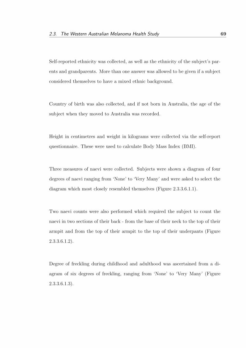
2.3. The Western Australian Melanoma Health Study 69
Self-reported ethnicity was collected, as well as the ethnicity of the subject’s par-
ents and grandparents. More than one answer was allowed to be given if a subject
considered themselves to have a mixed ethnic background.
Country of birth was also collected, and if not born in Australia, the age of the
subject when they moved to Australia was recorded.
Height in centimetres and weight in kilograms were collected via the self-report
questionnaire. These were used to calculate Body Mass Index (BMI).
Three measures of naevi were collected. Subjects were shown a diagram of four
degrees of naevi ranging from ‘None’ to ‘Very Many’ and were asked to select the
diagram which most closely resembled themselves (Figure 2.3.3.6.1.1).
Two naevi counts were also performed which required the subject to count the
naevi in two sections of their back - from the base of their neck to the top of their
armpit and from the top of their armpit to the top of their underpants (Figure
2.3.3.6.1.2).
Degree of freckling during childhood and adulthood was ascertained from a di-
agram of six degrees of freckling, ranging from ‘None’ to ‘Very Many’ (Figure
2.3.3.6.1.3).

70Chapter 2. Genetic Epidemiology of Malignant Melanoma: Susceptibility and
Prognosis in the WAMHS
Figure 2.3.3.6.1.1: Degrees of naevi from the WAMHS questionnaire
Figure 2.3.3.6.1.2: Number of naevi in two sections of the back from the WAMHS
questionnaire

2.3. The Western Australian Melanoma Health Study 71
Figure 2.3.3.6.1.3: Degree of freckling from the WAMHS questionnaire
Subjects were asked about their eye colour, skin colour and hair colour at age 18.
Skin reaction to the sun was also collected from subjects. These questions were
used as an indicator of how uncovered skin reacted to sun exposure in terms of
sunburn and tanning and were based on the Fitzpatrick scale [161].
Smoking history was collected, with ‘smoking’ defined as having smoked at least
one cigarette per day for a period of six months or more. Subjects were asked if
they had ever smoked, how long they smoked for, and how many cigarettes per
day they smoked.
A subject’s history of melanoma was ascertained through both the questionnaire
and WACR records. Subjects who identified themselves during the questionnaire
as having had more than one melanoma were classified as having a history of

72Chapter 2. Genetic Epidemiology of Malignant Melanoma: Susceptibility and
Prognosis in the WAMHS
melanoma. Similarly, subjects who had more than one primary melanoma diag-
nosis notified to the WACR were classified as having a history of melanoma. In
both instances, the number of melanomas diagnosed was also recorded. A sub-
ject’s history of other cancers, including other skin cancers, was also recorded.
Sunbed use was collected and was defined as having used a sunbed on more than
one occasion. The overall number of sunbed sessions and the locations of these
sessions were recorded.
A subject’s family history of melanoma was also collected. A family history of
melanoma was defined as having more than one first-degree relative (i.e. mother,
father, brother, sister) diagnosed with melanoma, as reported by the subject. In
addition, a family history of other skin cancers, and other cancers was also col-
lected.
Subjects were asked to recall the number of times they had been sunburnt during
three periods of their lives – from 5-12 years, from 13-19 years and from 20 years
onwards. Sunburn was separated into two questions – sunburn to cause pain for
more than two days and sunburn severe enough to cause blisters. These variables
had four levels – 0, 1-5, 6-10 and more than 10 times.
Time spent outdoors in warmer and cooler months during various age periods was
also collected. This included the number of hours spent outside and not under
any shade between 9am and 5pm.

2.3. The Western Australian Melanoma Health Study 73
2.3.3.6.2 Demographic and clinical variables
The majority of demographic and clinical variables were collected from the WACR.
The WACR collects extensive details regarding an individual’s melanoma diagno-
sis from pathology reports, including Breslow thickness, Clark’s level, sex, WACR
history of melanoma and date of melanoma diagnosis.
Breslow thickness was collected for the excised melanoma and was measured in
millimetres. In addition, another measure of the thickness of the excised melanoma
was collected – Clark’s level. The possible levels were II, III, IV and V, indicating
the layers of skin the melanoma had invaded. Clark’s level I refers to an in situ
melanoma and as subjects were recruited into the study based on diagnosis of an
invasive melanoma, no subjects were recruited into the study who had only been
diagnosed with a Clark’s level I melanoma.
Sex was collected from the WACR. Age at diagnosis was also collected and was
calculated as the date of diagnosis minus date of birth. Date of diagnosis is the
date at which the melanoma was fully or partially excised by a clinician.
Age at data collection was calculated as the date of the telephone questionnaire
minus date of birth. WACR history of invasive and in situ melanoma was also
collected, where WACR history of melanoma was defined as the subject having
had more than one primary melanoma notified to the WACR.

74Chapter 2. Genetic Epidemiology of Malignant Melanoma: Susceptibility and
Prognosis in the WAMHS
2.3.3.7 Sample size and response rates
At the conclusion of the data collection period, the WAMHS consisted of 1,643
consenting cases of melanoma. This consisted of 144 subjects who enrolled in
the pilot study, and 1,499 subjects who enrolled in the full-scale implementation
of the study. 73 of the 1,499 subjects withdrew or died prior to participation in
the study. Of the 1,426 subjects who remained enrolled in the full-scale study,
91.87% (n=1,310) completed Part 1 of the questionnaire, 91.87% (n=1,310) com-
pleted Part 2 of the questionnaire and 84.43% (n=1,204) gave a blood sample for
DNA and serum. 81.14% (n=1,157) of the subjects completed all parts of the
study.
Figure 2.3.3.7.1 depicts the final figures and rates for the study, including both
the pilot study and the full-scale implementations.
2.3.3.7.1 Consent, non-consent and non-response rates
Statistical analysis was performed to compare the subject characteristics between
consenting subjects and non-consenting subjects, and also consenting subjects and
non-responders. Non-consenting subjects were defined as those who returned a
consent form indicating they did not wish to participate in the study, and non-
responders were defined as subjects who did not return a consent form indicating
if they wished to participate.
In total, of the 3,420 individuals diagnosed with melanoma within the diagnosis
timeframe, 1,643 (48%) subjects consented to participate in the study, 644 (19%)
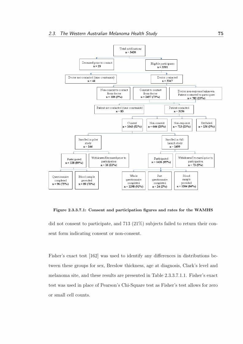
2.3. The Western Australian Melanoma Health Study 75
Figure 2.3.3.7.1: Consent and participation figures and rates for the WAMHS
did not consent to participate, and 713 (21%) subjects failed to return their con-
sent form indicating consent or non-consent.
Fisher’s exact test [162] was used to identify any differences in distributions be-
tween these groups for sex, Breslow thickness, age at diagnosis, Clark’s level and
melanoma site, and these results are presented in Table 2.3.3.7.1.1. Fisher’s exact
test was used in place of Pearson’s Chi-Square test as Fisher’s test allows for zero
or small cell counts.

76Chapter 2. Genetic Epidemiology of Malignant Melanoma: Susceptibility and
Prognosis in the WAMHS
Variable Consent Non-consent p-value No reply p-value
(n=1,643) (n=644) (n=713)
% [n] % [n] % [n]
Sex
Male 58.37 [959] 59.78 [385] 64.09 [457]
Female 41.63 [684] 40.22 [259] 0.57 35.91 [256] 0.0091
Breslow thickness, mm
0–1.00 71.94 [1182] 71.43 [460] 72.37 [516]
1.01–2.00 14.49 [238] 12.42 [80] 14.31 [102]
2.01–4.00 7.12 [117] 9.47 [61] 0.20 6.59 [47] 0.87
>4.00 3.77 [62] 3.26 [21] 4.49 [32]
Unknown 2.68 [44] 3.42 [22] 2.24 [16]
Age at diagnosis
18–29 2.31 [38] 1.70 [11] 8.56 [61]
30–44 13.94 [229] 8.85 [57] 25.95 [185]
45–59 32.56 [535] 25.47 [164] <0.0001 35.34 [252] <0.0001
60–74 40.54 [666] 42.24 [272] 23.98 [171]
75–80 10.65 [175] 21.74 [140] 6.17 [44]
Clark’s Level
II 36.76 [604] 37.42 [241] 38.71 [276]
III 25.63 [421] 22.98 [148] 23.56 [168]
IV 31.89 [524] 32.30 [208] 0.10 31.98 [228] 0.85
V 2.74 [45] 2.17 [14] 2.66 [19]
Unknown 2.98 [49] 5.12 [33] 3.09 [22]
Site
Head and neck 16.43 [270] 17.86 [115] 13.74 [98]
Trunk 34.04 [625] 39.60 [255] 37.03 [264]
Upper limb 23.25 [382] 22.05 [142] 0.63 25.95 [185] 0.39
Lower limb 21.85 [359] 20.34 [131] 22.86 [163]
Unknown 0.43 [7] 0.15 [1] 0.42 [3]
Table 2.3.3.7.1.1: Comparison of characteristics between consenting, non-consenting
and non-responding subjects
Analysis of consent versus non-consent found that the distributions of Breslow
thickness, sex, Clark’s level and site did not differ significantly. The frequency
distributions of these variables in consenters and non-consenters were similar.
However, the age of diagnosis distribution was significantly different (P<0.0001).

2.3. The Western Australian Melanoma Health Study 77
Analysis of consent versus non-response found that the distributions of Breslow
thickness, Clark’s level and site did not differ significantly. However, the sex
distribution was significantly different (P=0.0091), with a greater proportion of
males not responding (64.09%) versus consenting to participate (58.37%). The
age of diagnosis distribution also differed significantly between consenters and
non-responders (P<0.0001).
The differences in age distribution between consenters and non-consenters, and
consenters and non-responders was marked. In consenting individuals, the age
group 18 to 29 accounted for 2.31% of consenters. This was similar to the 1.70%
of non-consenters in this age category, however 8.56% of the non-responders were
aged between 18 to 29. This is a much larger proportion than would be expected.
Similar trends can be seen for the next two age groups – 30 to 44, and 45 to 59 –
with these age groups accounting for a smaller proportion of non-consenters, and
a larger proportion of non-responders. In the older age groups, the opposite trend
was observed, with the two age groups 60 to 74 and 75 to 80 accounting for a
larger proportion of non-consenters and a smaller proportion of non-responders.
These results suggest that individuals who did not respond tended to be younger
than individuals who consented. In addition, non-consenters appeared to be older
than consenting individuals. This may indicate that younger individuals who did
not wish to participate in the Study were less likely to respond, where as older
individuals who did not wish to participate were more likely to respond indicating
their non-consent.

78Chapter 2. Genetic Epidemiology of Malignant Melanoma: Susceptibility and
Prognosis in the WAMHS
2.3.3.8 Characteristics of participants
Table 2.3.3.8.1 shows demographic, clinical and questionnaire characteristics of
WAMHS participants who completed either Part 1 or Part 2 of the questionnaire.
These characteristics are stratified by sex and compared using Fisher’s exact test.
Participants who consented to participate in the study, but did not complete ei-
ther of the questionnaires are excluded from this table.
The sex distribution was skewed, with 58.17% of the sample male. Approximately
three-quarters of subjects were aged over 45, and the age distribution differed be-
tween sexes (P<0.0001). There were more females aged between 18 and 59 and
more males aged between 60 and 80.
Approximately 70% (n=944) of subjects had melanomas diagnosed less than 1 mm
thick, and only 3.55% (n=47) had melanomas thicker than 4 mm. Breslow thick-
ness differed between the sexes, with 69.57% (n=535) of males having melanomas
less than 1 mm thick, compared to 73.96% (n=409) of females. In addition, males
were more than twice as likely (4.55% compared to 2.17%) of having melanomas
more than 4 mm thick.
The most common melanoma site was the trunk, with 38.05% (n=203) of melanoma
diagnoses. The least common melanoma site was the head and neck region
(15.36%). Site distributions differed significantly between sexes (P<0.0001), with
male participants more likely to have melanomas diagnosed on their head, neck
and trunk, and females on their upper and lower limbs. The greatest difference
due to sex was observed at the lower limb site, with females approximately 2.4

2.3. The Western Australian Melanoma Health Study 79
times more likely to be diagnosed with melanomas on their lower limbs compared
to males.
The majority of subjects considered themselves to be Caucasian, with 50% (n=813)
considering themselves to be Caucasian of English background, and 27% (n=442)
Caucasian with Scottish, Irish or Welsh background. Approximately three-quarters
of subjects were born in Australia, with approximately 14% (n=182) born in Eng-
land, Ireland, Scotland, or Wales.
Over 90% (n=1,198) of subjects had some ability to tan, while only 8.47% (n=112)
reported that their skin never tanned, and only freckled. Men appeared to have
a greater ability to tan (P<0.0001) and also had a lower propensity to burn
(P<0.0001). This may be a result of self-reporting errors, with men more likely to
under-report their burning tendency, however there have not been any published
studies which support this theory.
Approximately 18% (n=237) of subjects considered their skin colour to be very
fair, 10.59% (n=140) had red hair at age 18, and 42.51% (n=562) had blue eyes.
Both hair (P<0.0001) and eye colour (P<0.0001) differed between sexes, with
men more likely to have black hair, and women more likely to have red hair. Men
were also more likely to have blue or brown eyes, with women more likely to have
hazel or green eyes. There is no scientific evidence for men and women having
different coloured eyes or hair, and this difference may be a result of reporting bias.
Degree of freckling decreased from childhood to adulthood. 23.45% (n=310) of

80Chapter 2. Genetic Epidemiology of Malignant Melanoma: Susceptibility and
Prognosis in the WAMHS
subjects had no freckling during childhood, which increased to 29.05% (n=384)
during adulthood. Similarly, 9.91% (n=131) of subjects considered themselves to
have ‘Many’ or ‘Very many’ freckles during childhood, which more than halved to
4.91% (n=65) in adulthood. Sex differences for childhood and adulthood freckling
also existed, with males less likely to have freckling compared to females for both
periods (P<0.0001). It is possible that this is due to differences in reporting by
males and females.
Another measure of sun exposure - blistering sunburn - also decreased from child-
hood to adolescence. 8.09% (n=107) of subjects reported more than 10 episodes of
blistering sunburn during childhood, which decreased to 5.98% (n=79) in adoles-
cence. Similarly, the percentage of subjects who reported no episodes of blistering
sunburn increased from childhood to adolescence, from 38.28% (n=506) in child-
hood, to 43.72% (n=578) in adolescence.
VariableWAMHS Males Females p-value
(n=1,322) (n=769) (n=553)
% [n] % [n] % [n]
Breslow thickness, mm
0–1.00 71.41 [944] 69.57 [535] 73.96 [409]
1.01–2.00 15.13 [200] 15.60 [200] 14.47 [80]
2.01–4.00 7.11 [94] 8.07 [94] 5.79 [32] 0.03
>4.00 3.55 [47] 4.55 [47] 2.17 [12]
Unknown 2.80 [37] 2.21 [17] 3.61 [20]
Age at diagnosis
18–29 2.19 [29] 1.43 [11] 3.26 [18]
30–44 14.14 [187] 9.75 [75] 20.25 [112]
45–59 33.06 [437] 30.94 [238] 35.99 [199] <0.0001
60–74 40.47 [535] 45.90 [353] 32.91 [182]
75–80 10.14 [134] 11.96 [92] 7.59 [42]
Clarks Level
II 36.23 [479] 36.02 [277] 36.53 [202]
III 25.72 [340] 24.58 [189] 27.31 [151]
Continued on Next Page. . .

2.3. The Western Australian Melanoma Health Study 81
Table 2.3.3.8.1 – Continued
VariableWAMHS Males Females p-value
(n=1,322) (n=769) (n=553)
IV 32.45 [429] 34.59 [266] 29.48 [163] 0.44
V 2.34 [31] 2.21 [17] 2.53 [14]
Unknown 0.45 [6] 0.52 [4] 0.26 [2]
Site
Head and neck 15.36 [203] 18.73 [144] 10.67 [59]
Trunk 38.05 [503] 46.69 [359] 26.04 [144]
Upper limb 23.68 [313] 19.90 [153] 28.93 [160] <0.0001
Lower limb 22.62 [299] 14.20 [110] 34.18 [189]
Unknown 0.30 [4] 0.39 [3] 0.18 [1]
Self-reported ethnicity
Caucasian - English 50.03 [813] 50.58 [478] 49.26 [335]
Caucasian - Scottish, Irish, Welsh 27.20 [442] 27.83 [263] 26.32 [179]
Caucasian - Northern European 7.69 [125] 8.47 [80] 6.62 [45]
Caucasian Southern European 2.52 [41] 1.69 [16] 3.68 [25]
Caucasian Eastern European 0.86 [14] 0.95 [9] 0.74 [5] 0.02
Caucasian Other 11.08 [180] 9.73 [92] 12.94 [88]
Indigenous 0.12 [2] 0.21 [2] 0.00 [0]
Middle Eastern 0.18 [3] 0.32 [2] 0.00 [0]
Pacific Islander 0.25 [4] 0.11 [1] 0.44 [3]
African 0.06 [1] 0.11 [1] 0.00 [0]
Place of Birth
Australia 74.58 [986] 75.68 [582] 73.06 [404]
New Zealand 4.31 [57] 3.77 [29] 5.06 [28]
England 10.82 [143] 10.40 [80] 11.39 [63]
Scotland/Ireland/Wales 2.95 [39] 2.99 [23] 2.89 [16] 0.78
Northern Europe 2.12 [28] 2.08 [16] 2.17 [12]
Other 4.31 [57] 4.42 [34] 4.16 [23]
Missing 0.91 [12] 0.65 [5] 1.27 [7]
Naevi
None 10.67 [141] 10.40 [80] 11.03 [61]
Few 35.02 [463] 34.20 [263] 36.17 [200]
Some 37.97 [502] 37.97 [292] 37.97 [210] 0.62
Many 15.20 [201] 15.99 [123] 14.10 [78]
Missing 1.14 [15] 1.43 [11] 0.72 [4]
Ability to tan
Very brown 12.55 [166] 15.47 [119] 8.50 [47]
Moderate brown 44.33 [586] 49.15 [378] 37.61 [208]
Slight tan 33.74 [446] 29.78 [229] 39.24 [217] <0.0001
No tan / freckle only 8.47 [112] 4.55 [35] 13.92 [77]
Missing 0.91 [12] 1.04 [8] 0.72 [4]
Continued on Next Page. . .

82Chapter 2. Genetic Epidemiology of Malignant Melanoma: Susceptibility and
Prognosis in the WAMHS
Table 2.3.3.8.1 – Continued
VariableWAMHS Males Females p-value
(n=1,322) (n=769) (n=553)
Propensity to burn
Never burn, always tan 2.12 [28] 2.73 [21] 1.27 [7]
Sometimes burn, usually tan 50.76 [671] 55.40 [426] 44.30 [245]
Usually burn, sometimes tan 22.69 [300] 22.24 [171] 23.33 [129] <0.0001
Always burn, never tan 23.52 [311] 18.60 [143] 30.38 [168]
Missing 0.91 [12] 1.04 [8] 0.72 [4]
Skin Colour
Olive/brown 7.72 [102] 8.45 [65] 6.69 [37]
Fair 73.37 [970] 74.51 [573] 71.79 [397] 0.14
Very fair 17.93 [237] 15.99 [123] 20.61 [114]
Missing 0.98 [13] 1.04 [8] 0.90 [5]
Hair colour at age 18
Black 5.45 [72] 7.93 [61] 1.99 [11]
Dark brown 26.85 [355] 26.66 [205] 27.12 [150]
Grey 1.82 [24] 2.99 [23] 0.18 [1]
Light/mouse brown 33.59 [444] 31.73 [244] 36.17 [200] <0.0001
Fair/blonde 20.73 [274] 21.07 [162] 20.25 [112]
Red 10.59 [140] 8.58 [66] 13.38 [74]
Missing 0.98 [13] 1.04 [8] 0.90 [5]
Eye Colour
Brown 14.75 [195] 16.12 [124] 12.84 [71]
Hazel 22.77 [301] 19.51 [150] 27.31 [151]
Green 13.62 [180] 12.09 [93] 15.73 [87] <0.0001
Grey 5.37 [71] 5.07 [39] 5.79 [32]
Blue 42.51 [562] 46.16 [355] 37.43 [207]
Missing 0.98 [13] 1.04 [8] 0.90 [5]
Freckling, Childhood
None 23.45 [310] 27.57 [212] 17.72 [98]
Very Few 31.39 [415] 33.42 [257] 28.57 [158]
Few 20.42 [270] 19.90 [153] 21.16 [117]
Some 13.92 [184] 11.44 [88] 17.36 [96] <0.0001
Many/Very Many 9.91 [131] 6.63 [51] 14.47 [80]
Missing 0.91 [12] 1.04 [8] 0.72 [4]
Freckling, Adulthood
None 29.05 [384] 35.50 [273] 20.07 [111]
Very Few 37.90 [501] 39.27 [302] 35.99 [199]
Few 16.49 [218] 13.39 [103] 20.80 [115] <0.0001
Some 10.74 [142] 7.41 [57] 15.37 [85]
Many/Very Many 4.91 [65] 3.38 [26] 7.05 [39]
Missing 0.91 [12] 1.04 [8] 0.72 [4]
Continued on Next Page. . .

2.3. The Western Australian Melanoma Health Study 83
Table 2.3.3.8.1 – Continued
VariableWAMHS Males Females p-value
(n=1,322) (n=769) (n=553)
Blistering Sunburn, 5-12 years
0 times 38.28 [506] 35.24 [271] 42.50 [235]
1–5 times 40.54 [536] 42.26 [325] 38.16 [211]
6–10 times 10.06 [133] 11.05 [85] 8.68 [48]
> 10 times 8.09 [107] 8.84 [68] 7.05 [39] 0.07
Don’t know 1.74 [23] 1.43 [11] 2.17 [12]
Missing 1.29 [17] 1.17 [9] 1.45 [8]
Blistering Sunburn, 13-19 years
0 times 43.72 [578] 44.73 [344] 42.32 [234]
1–5 times 40.32 [533] 40.45 [311] 40.14 [222]
6–10 times 8.09 [107] 8.06 [62] 8.14 [45] 0.65
> 10 times 5.98 [79] 5.07 [39] 7.23 [40]
Don’t know 0.60 [8] 0.52 [4] 0.72 [4]
Missing 1.29 [17] 1.17 [9] 1.45 [8]
Table 2.3.3.8.1: Questionnaire, demographic and clinical characteristics of WAMHS sample, strat-
ified by sex
2.3.3.9 WAMHS sample summary
The WAMHS is a population-based case collection comprised of individual melanoma
cases recruited from the WACR. Phenotypic, demographic, clinical, and biospeci-
men data were collected as part of this study, and form a comprehensive resource
for melanoma researchers.
The WAMHS sample consisted of 1,643 consenting cases of melanoma diagnosed
between January 2006 and September 2009. Of these cases, 144 (8.76%) par-
ticipated in the pilot study, and 1,499 (91.24%) participated in the full-scale
implementation. Of consenting participants from the pilot study, 87 (67.97%)
completed both the questionnaire and donated a blood sample. After changes to
the study, and the implementation of the full-launch study, 1,157 (81.14%) partic-
84Chapter 2. Genetic Epidemiology of Malignant Melanoma: Susceptibility and
Prognosis in the WAMHS
ipants completed the questionnaire and donated a blood sample. This increase in
completion rates may be attributed to the shorter questionnaire and the change
to administering the questionnaire by telephone interview.
Analysis of consent versus non-consent revealed that the age distributions were
significantly different, with a greater proportion of subjects aged between 45 and
59 consenting to the study, and a lower proportion of subjects aged between 75
and 80 consenting. The lower proportion of older subjects consenting may be as
participation in a study can be particularly difficult for older individuals for many
reasons, e.g. they may be less mobile and suffering from poorer health.
Analysis of consent versus non-response found that the sex distribution was signif-
icantly different, with a greater proportion of males failing to respond, compared
to males who consented to participate. In addition, the age distribution differed
significantly, with more subjects aged less than 60 failing to respond, and more
individuals over 60 responding.
Analysis of the WAMHS sample revealed that the demographic and clinical vari-
ables, age at diagnosis, Breslow thickness, and site distributions, differed between
sexes. There were more females aged between 18 and 59 and more males aged be-
tween 60 and 80 in the study. Females were more likely to have thinner melanomas
(< 1 mm), while males were more likely to have thicker melanomas (> 4 mm).
Male subjects were more likely to have melanomas diagnosed on their head, neck
and trunk, while women were more likely to have melanomas diagnosed on their
upper and lower limbs. This site distribution is similar to those observed in pre-

2.3. The Western Australian Melanoma Health Study 85
vious studies [90,163].
Several questionnaire variables differed between sexes, including ability to tan,
propensity to burn, hair and eye colour. Males appeared to have a greater ability
to tan, and a lower propensity to burn. In addition, males were more likely to
have black hair, compared to females, and females were more likely to have red
hair, compared to males. Eye colour also differed between the sexes, with males
more likely to have brown or blue eyes, and females more likely to have hazel or
green eyes.
The imbalance in self-reported variables in the WAMHS sample between men and
women, such as hair and eye colour, does not appear to have a scientific basis.
These differences may be explained by systematic self-report bias. For example,
women in this sample may be more likely than men to select their eye colour as
green. This may have implications if these self-reported variables were included
as covariates in analyses.
2.3.4 WAMHS sub-sample used in this thesis
2.3.4.1 Introduction
The genetic association analyses presented in this thesis, which are found in Sec-
tions 2.4 (please see page 111) and 2.5 (please see page 131), use a subset of
the WAMHS sample. This subset consists of 800 unrelated individuals who had
completed both study questionnaires by February 2010, and had donated the
blood sample by September 2009. In addition, these subjects were chosen as they
had a Breslow thickness recorded and were of Caucasian descent. A subject was
86Chapter 2. Genetic Epidemiology of Malignant Melanoma: Susceptibility and
Prognosis in the WAMHS
categorised as Caucasian if they described both themselves and their parents as
Caucasian.
Blood samples from these 800 participants were genotyped for 42 SNPs, and the
selection of these SNPs is described in this section. This section also includes
methods for the descriptive analyses of both study variables and genotypic data,
and also presents the results of these descriptive analyses. In addition, the gener-
alisability of this sample to the entire population of melanoma diagnoses within
the diagnosis timeframe is investigated.
2.3.4.2 SNP selection
Forty two melanoma risk SNPs were chosen as they had been identified as vali-
dated melanoma-risk SNPs, or were in genes which have been validated as melanoma-
risk genes. Nineteen SNPs were tagged from three genes – MC1R, BRAF and
EGF. Variation in all three genes was captured by choosing tag-SNPs using a
pairwise tagging approach in the Haploview software package [164]. Gene coordi-
nates were determined by using the University of California Santra Cruz Genome
Browser Gateway [165], with the coordinates used for tagging including 10 kb
upstream and 10 kb downstream of each gene. Haploview tagger [166] was used
to select a set of tag-SNPs which captured maximal variation in the gene. The
minimum minor allele frequency for selected SNPs was set at 5% and the thresh-
old for LD was set to r2=0.80.
Table 2.3.4.2.1 shows the three genes tagged in Haploview, the coordinates used
for tagging, and the tag-SNPs successfully genotyped in the WAMHS sample.
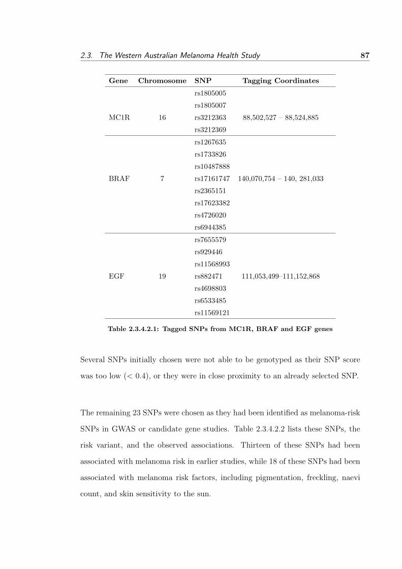
2.3. The Western Australian Melanoma Health Study 87
Gene Chromosome SNP Tagging Coordinates
rs1805005
rs1805007
MC1R 16 rs3212363 88,502,527 – 88,524,885
rs3212369
rs1267635
rs1733826
rs10487888
BRAF 7 rs17161747 140,070,754 – 140, 281,033
rs2365151
rs17623382
rs4726020
rs6944385
rs7655579
rs929446
rs11568993
EGF 19 rs882471 111,053,499–111,152,868
rs4698803
rs6533485
rs11569121
Table 2.3.4.2.1: Tagged SNPs from MC1R, BRAF and EGF genes
Several SNPs initially chosen were not able to be genotyped as their SNP score
was too low (< 0.4), or they were in close proximity to an already selected SNP.
The remaining 23 SNPs were chosen as they had been identified as melanoma-risk
SNPs in GWAS or candidate gene studies. Table 2.3.4.2.2 lists these SNPs, the
risk variant, and the observed associations. Thirteen of these SNPs had been
associated with melanoma risk in earlier studies, while 18 of these SNPs had been
associated with melanoma risk factors, including pigmentation, freckling, naevi
count, and skin sensitivity to the sun.

88
Chapter
2.G
eneticE
pidemiology
ofM
alignantM
elanoma:
Susceptibility
andP
rognosisin
theW
AM
HS
Gene SNP Risk Allele Association
CDC91L1 rs910873 A Increased melanoma risk [106,107]
MC1R rs258322 A Increased melanoma risk [106,124]
MYH7B rs1885120 C Increased melanoma risk [106,107]
TYR rs1042602 C Freckling [109], increased melanoma risk [106]
TYR rs1393350 A Blonde hair [109], green eyes [109], increased skin sensitivity to sun [109], increased melanoma risk [106]
TYRP1 rs1408799 C Blue eyes [109], increased skin sensitivity to sun [109], increased melanoma risk [108]
KITLG rs12821256 C Blonde hair [109]
SLC2A4 rs12896399 T Blonde hair [109], increased skin sensitivity to sun [109]
IRF4 rs1540771 A Brown hair [109], increased freckling [109], increased skin sensitivity to sun [109]
IRF4 rs12203592 T Blonde hair [124], lighter eye and skin colour [124], reduced tanning ability [124]
TPCN2 rs35264875 T Blonde hair [167]
TPCN2 rs3829241 A Blonde hair [167]
OCA2 rs1800407 G Blue eyes [168]
OCA2 rs1800401 A Black or brown eyes [169]
OCA2 rs7495174 A Blue or green eyes [109,168]
HERC2 rs12913832 G Blue eyes [170,171]
TP53 rs1042522 C Increased melanoma risk [172]
MTAP rs4636294 A Increased melanoma risk [105,106], increased naevi count, [105]
MTAP rs10757257 G Increased melanoma risk [105,106], increased naevi count [105]
MTAP rs7023329 A Increased melanoma risk [105,106], increased naevi count [105]
MTAP rs1011970 T Increased melanoma risk [106]
PLA2G6 rs2284063 A Increased melanoma risk [105,106], increased naevi count [105]
PLA2G6 rs132985 C Increased melanoma risk [105], increased naevi count [105]
Table 2.3.4.2.2: Reported melanoma-risk associations between genotyped SNPs and melanoma-risk factors
2.3. The Western Australian Melanoma Health Study 89
2.3.4.3 Laboratory methods
The methods to prepare the DNA for genotyping and the genotyping methods are
described below.
2.3.4.3.1 DNA preparation
DNA extraction and sample preparation was performed by the WADB, Perth.
DNA was extracted at room temperature from the buffy coat using the phenol-
chloroform method, and then suspended in TE buffer. DNA was quantitated using
a ND-1000 Nanodrop Spectrophotometer to ensure that sufficient quantities of un-
contaminated DNA were present. DNA samples of > 20 ng/µL concentration were
diluted to approximately 2 ng/µL using the PerkinElmer Multiprobe II pipetting
robot. Two microlitres of each DNA sample was dispersed into each well of a
96-well plate using the Beckman Coulter biomek FX machine, resulting in 4 ng
of DNA sample per well. Plates were left to dry at room temperature overnight
prior to use.
2.3.4.3.2 Genotyping
DNA samples were genotyped by the PathWest Molecular Genetics Service, Perth.
All genotyping was performed using Illumina GoldenGate Assays. The DNA sam-
ple was first activated, and the DNA was added to the oligonucleotides and then
hybridised. Three oligonucleotides were used for each SNP locus. Two oligonu-
cleotides were specific to each allele of the SNP (‘allele specific oligo’), and the
third hybridised at a site downstream from the SNP site (‘locus specific oligo’).
Following hybridisation, wash steps were performed to reduce excess and mis-
hybridised oligonucleotides. The allele specific oligo joined with the locus specific

90Chapter 2. Genetic Epidemiology of Malignant Melanoma: Susceptibility and
Prognosis in the WAMHS
oligo, to provide information regarding the genotype present at the SNP site. A
set of fluorescent Polymerase Chain Reaction (PCR) primers were added and PCR
occurred, generating fluorescent products. These products were combined with
Illumina beads on the Sentrix Array Matrix, combining with their matching bead.
The fluorescence of each bead was analysed on the BeadArray Reader, generating
automated genotype clustering and calling.
Genotyping quality control was performed in several steps. Each plate contained
a negative control sample (water) and a positive control CEPH trio sample. If
these controls failed, then the plate was re-genotyped. The controls did fail on one
plate and this was re-genotyped with no further errors. Additionally, genotyping
was repeated on 10% of the samples to ensure accuracy which resulted in 100%
concordance.
2.3.4.4 Methods for descriptive analyses
This section describes the methods for descriptive statistics of both study variables
and genotypic data.
2.3.4.4.1 Descriptive statistics of study variables
Descriptive statistics for the phenotypic and genotypic data were calculated us-
ing the statistical package, R. Means and standard deviations were calculated for
Normally distributed continuous variables, and medians and interquartile range
(IQR) were calculated for skewed continuous variables. Counts and percentages
were calculated for categorical and dichotomous variables. A histogram of Bres-
low thickness was examined to identify any deviations from Normality. Breslow

2.3. The Western Australian Melanoma Health Study 91
thickness was transformed by taking the natural log, loge(Breslow thickness) and
the resulting histogram was examined. Due to the skewness of Breslow thickness,
both the geometric mean and and 95% confidence intervals were calculated.
2.3.4.4.2 Descriptive statistics of genotype data
Genotype and allele frequencies were calculated using R. Consistency of genotype
distributions with HWE in the WAMHS sub-sample were examined at each SNP
locus using Fisher’s exact test.
2.3.4.5 Results for descriptive analyses
2.3.4.5.1 Phenotypic data
This sub-sample consisted of 800 individuals who were diagnosed with melanoma
from the WAMHS. Questionnaire-based characteristics and demographic and clin-
ical characteristics of this sub-sample are presented in Table 2.3.4.5.1.1 and Table
2.3.4.5.1.2 respectively.
Variable Study Population
(n=800)
Continuous variable, mean (SD)
BMI, kg/m2 27.45 (5.22)
Continuous variables, median (IQR)
Number of naevi - upper back 4.00 (9.00)
Number of naevi - lower back 5.00 (13.00)
Smoking, pack years 11.63 (21.95)
Dichotomous and categorical variables, % [n]
Place of Birth
Australia 76.00 [608]
England 10.50 [84]
New Zealand 4.25 [34]
Continued on Next Page. . .

92Chapter 2. Genetic Epidemiology of Malignant Melanoma: Susceptibility and
Prognosis in the WAMHS
Table 2.3.4.5.1.1 – Continued
Variable Study Population
(n=800)
Scotland/Ireland/Wales 3.25 [26]
Africa 2.38 [19]
Northern Europe 2.12 [17]
Other 1.50 [12]
Smoking
Never smoked 53.75 [430]
Ex-smokers 40.25[322]
Current Smokers 6.00 [48]
Naevi
None 11.88 [95]
Few 36.00 [288]
Some 38.50 [308]
Many 13.50[108]
Missing 0.02[1]
Sunbed use
Yes 11.38 [91]
No 88.25 [706]
Don’t know 0.37 [3]
Self-reported history of melanoma
Yes 27.37 [219]
No 72.63 [581]
WACR reported history of melanoma
Yes 21.13 [169]
No 78.87 [631]
Self-reported history of SCC or BCC
Yes 45.38 [363]
No 45.50 [364]
Don’t know 9.12 [71]
Ability to tan
Very brown 12.37 [99]
Moderate tan 44.50 [356]
Slight tan 34.00 [272]
No tan/freckle only 9.13 [73]
Propensity to burn
Continued on Next Page. . .

2.3. The Western Australian Melanoma Health Study 93
Table 2.3.4.5.1.1 – Continued
Variable Study Population
(n=800)
Never burn, always tan 2.25 [18]
Sometimes burn, usually tan 51.12 [409]
Usually burn, sometimes tan 24.13 [193]
Always burn, never tan 22.50 [180]
Skin colour
Olive/brown 7.00 [56]
Fair 74.30 [594]
Very fair 18.70 [150]
Hair colour at age 18
Black 5.50 [44]
Dark brown 29.38 [235]
Grey 2.25 [18]
Light/mouse brown 33.62 [269]
Fair/blonde 20.37 [163]
Red 8.88 [71]
Eye colour
Brown 14.12 [113]
Hazel 24.25 [194]
Green 14.00 [112]
Grey 6.13 [49]
Blue 41.50 [332]
Degree of freckling - childhood
None 24.38 [195]
Very few 33.00 [264]
Few 20.25 [162]
Some 12.87 [103]
Many/Very many 9.50 [76]
Degree of freckling - adulthood
None 30.38 [243]
Very few 38.25 [306]
Few 16.75 [134]
Some 10.62 [85]
Many/Very many 4.00 [32]
Family history of melanoma
Yes 23.25 [186]
Continued on Next Page. . .

94Chapter 2. Genetic Epidemiology of Malignant Melanoma: Susceptibility and
Prognosis in the WAMHS
Table 2.3.4.5.1.1 – Continued
Variable Study Population
(n=800)
No 76.75 [614]
Sunburn causing blisters, 5–12 years
0 times 39.75 [318]
1–5 times 39.63 [317]
6–10 times 10.50 [84]
> 10 times 8.00 [64]
Don’t know 2.12[17]
Sunburn causing blisters, 13–19 years
0 times 43.25 [346]
1–5 times 42.00 [336]
6–10 times 8.88 [71]
> 10 times 5.37 [43]
Don’t know 0.50 [4]
Sunburn causing blisters, > 20 years
0 times 69.38 [555]
1–5 times 25.37 [203]
6–10 times 2.63 [21]
> 10 times 2.37 [19]
Don’t know 0.25 [2]
Table 2.3.4.5.1.1: Questionnaire-based characteristics of subjects in the WAMHS sub-
sample
All 800 subjects used in this analysis were of self-reported Caucasian descent.
Individuals were classified as Caucasian if they considered their ethnicity to be
‘Caucasian’ and if they considered both their parents to be ‘Caucasian’. The
sex distribution was skewed with 56.12% males and 43.88% females. The median
age at diagnosis was 62.67, while the average age at data collection was 63.84
years. This corresponds to a median lag-time of approximately 14 months be-
tween melanoma diagnosis and completion of the study questionnaire.

2.3. The Western Australian Melanoma Health Study 95
VariableStudy Population
(n=800)
Continuous variable, geometric mean (95% CI)
Breslow thickness, mm 0.73 (0.69, 0.77)
Continuous variables, median (IQR)
Age at melanoma diagnosis, years 62.67 (16.86)
Age at data collection, years 63.84 (16.77)
Dichotomous and categorical variables, % [n]
Sex
Male 56.12 [449]
Female 43.88 [351]
Clark’s Level
II 36.25 [290]
III 26.00 [208]
IV 33.87 [271]
V 2.75 [22]
Unknown 1.13 [9]
Melanoma Site
Head and neck 17.00 [136]
Trunk 38.25 [306]
Upper limb 23.37 [187]
Lower limb 21.38 [171]
Table 2.3.4.5.1.2: Demographic and clinical characteristics of subjects in the
WAMHS sub-sample
Mean Breslow thickness was 1.11 mm; the distribution of which was highly skewed
(see Figure 2.3.4.5.1.1), with a median of 0.65 mm, indicating that half of WAMHS
subjects had melanomas less than 0.65 mm. A natural log transformation of
Breslow thickness resulted in a more Normal-appearing histogram (see Figure
2.3.4.5.1.2). When back-transformed, the geometric mean of Breslow thickness
was 0.73 (95%CI = 0.69, 0.77).
Melanomas were approximately evenly distributed through Clark’s Levels II, III

96Chapter 2. Genetic Epidemiology of Malignant Melanoma: Susceptibility and
Prognosis in the WAMHS
Figure 2.3.4.5.1.1: Histogram of the distribution of Breslow thickness in the
WAMHS.
and IV, while only a very small percentage of melanomas (2.75%) had a Clark’s
level of V. A large percentage (38.25%) of melanomas were located on the trunk,
with the lowest percentage of melanomas located on the head and neck regions
(17.00%).
Approximately three-quarters of subjects were born in Australia, with 10.50%
(n=84) born in England, and 4.25% (n=34) born in New Zealand. 53.75% (n=430)
of subjects had not smoked for a period of greater than six months, with approx-

2.3. The Western Australian Melanoma Health Study 97
Figure 2.3.4.5.1.2: Histogram of the distribution of log-transformed Breslow thick-
ness in the WAMHS
imately 6% (n=48) of all subjects currently smoking. Mean BMI was calculated
as 27.45 kg/m2.
Fewer naevi were present on the upper back (median=4), compared to the lower
back (median=5). The majority of subjects (74.59%) considered themselves to
have ‘Few’ or ‘Some’ naevi, while only 11.88% (n=95) had ‘None’. The degree
of freckling from childhood to adulthood decreased, with 30.38% (n=243) of sub-
jects recording no freckling during adulthood, decreasing to 24.38% (n=195) of

98Chapter 2. Genetic Epidemiology of Malignant Melanoma: Susceptibility and
Prognosis in the WAMHS
subjects in childhood. Similarly, 9.50% (n=76) of subjects considered themselves
to have ‘Many’ or ‘Very Many’ freckles in childhood, which more than halved by
adulthood to 4.00% (n=32).
27.37% (n=219) of individuals reported to have had more than one melanoma
diagnosed, however, records from the WACR indicated that only 21.13% (n=169)
of individuals had more than one melanoma diagnosis notified to the WACR. The
concordance between these two histories was moderate (Cohen’s kappa of 0.54).
Of the 169 individuals with a WACR history of melanoma, 44 (26%) individuals
did not report to the WAMHS that they had been diagnosed with more than
one melanoma. This may be as they were unaware of additional diagnoses, par-
ticularly if more than one melanoma was excised on the same day. Similarly, of
the 219 individuals who reported to have a history of melanoma, the WACR did
not have 94 (43%) of these melanomas recorded. This may be due to individuals
falsely stating they had a history of melanoma, or the WACR may not have been
notified of all melanoma diagnoses, which may occur if the melanomas were diag-
nosed outside of Australia. However, it appears more likely that individuals may
have over- and under-stated their melanoma diagnoses.
45.38% (n=363) of individuals reported to have been diagnosed with either an
SCC or BCC, 45.50% (n=364) reported not to have been diagnosed with an SCC
or BCC, with the remaining 9% (n=71) unable to recall this information. It has
been estimated that by the age of 70 years, 69% of males and 60% of females in
Australia will have been diagnosed with an SCC or BCC [281]. Therefore, with a
mean age of 63 at data collection, this rate of SCC and BCC diagnoses appears
to be a reasonable estimate.

2.3. The Western Australian Melanoma Health Study 99
Approximately 23% of individuals reported to have a first degree relative diag-
nosed with melanoma. This was self-reported and not validated. This is consid-
erably higher than other estimates of family history [93] and may be due to in-
dividuals with melanoma falsely believing they have a family history of melanoma.
Nearly half of all subjects had blue eyes (41.50%), and approximately 9% had red
hair at age 18. The majority of subjects considered their skin colour to be ‘Fair’
or ‘Very fair’ (93.00%), with the remaining 7.00% having ‘Olive’ or ‘Brown’ skin.
Approximately one quarter of subjects responded that they ‘Always burn, never
tan’, while only 2.25% (n=18) of subjects indicated that they ‘Never burn, always
tan’. Approximately 75% (n=628) of subjects indicated that after repeated sun
exposure, they develop a ‘Slight or moderate tan’, while 12.37% (n=99) develop
a ‘Very brown tan’, with 9.13% (n=73) indicating that they never tan and only
develop freckles.
Approximately 40% (n=318) of individuals did not have any incidents of sunburn
causing blisters when aged 5 to 12 years old. This increased to 43.25% (n=346)
and 69.38% (n=555) for the periods 13 to 19, and over 20 years of age, respectively.
The number of individuals who were sunburnt in each age group decreased as the
number of times sunburnt increased. 8.00% (n=64) of individuals were sunburnt
more than 10 times between the ages of 5 and 12, and this decreased to 5.37%
(n=43) and 2.37% (n=19) for the periods 13 to 19, and over 20 years of age,
respectively. In addition, 11.38% (n=91) of subjects had used a sunbed at some
time in their life.

100Chapter 2. Genetic Epidemiology of Malignant Melanoma: Susceptibility and
Prognosis in the WAMHS
2.3.4.5.2 Genotypic data
Genotype and allele frequencies and counts for the 42 genotyped SNPs are pre-
sented in Table 2.3.4.5.2.1, along with HapMap-CEU minor allele frequencies.
Included in Table 2.3.4.5.2.1 is the exact p-value for the HWE test for each SNP.
Thirty seven of the 42 genotype distributions were consistent with HWE. How-
ever, five genotypic distributions (IRF4 rs12203592, BRAF rs12676365, BRAF
rs6944385, EGF rs929446 and EGF rs11569121) were not in HWE at the 5% level
of significance.
Only three of the 42 SNPs had MAF less than 5%, and 12 SNPS had MAF less
than 10%, indicating that the majority of the SNPS were fairly common.
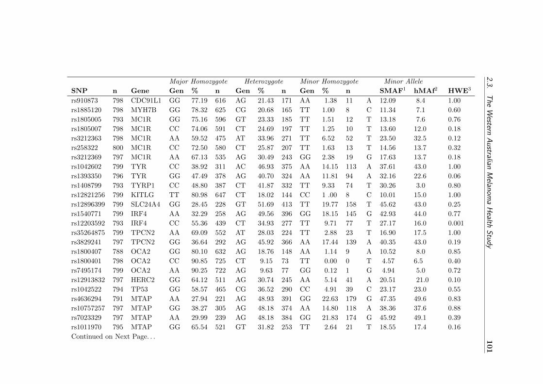
2.3.T
heW
esternA
ustralianM
elanoma
Health
Study
101
Major Homozygote Heterozygote Minor Homozygote Minor Allele
SNP n Gene Gen % n Gen % n Gen % n SMAF1 hMAf2 HWE3
rs910873 798 CDC91L1 GG 77.19 616 AG 21.43 171 AA 1.38 11 A 12.09 8.4 1.00
rs1885120 798 MYH7B GG 78.32 625 CG 20.68 165 TT 1.00 8 C 11.34 7.1 0.60
rs1805005 793 MC1R GG 75.16 596 GT 23.33 185 TT 1.51 12 T 13.18 7.6 0.76
rs1805007 798 MC1R CC 74.06 591 CT 24.69 197 TT 1.25 10 T 13.60 12.0 0.18
rs3212363 798 MC1R AA 59.52 475 AT 33.96 271 TT 6.52 52 T 23.50 32.5 0.12
rs258322 800 MC1R CC 72.50 580 CT 25.87 207 TT 1.63 13 T 14.56 13.7 0.32
rs3212369 797 MC1R AA 67.13 535 AG 30.49 243 GG 2.38 19 G 17.63 13.7 0.18
rs1042602 799 TYR CC 38.92 311 AC 46.93 375 AA 14.15 113 A 37.61 43.0 1.00
rs1393350 796 TYR GG 47.49 378 AG 40.70 324 AA 11.81 94 A 32.16 22.6 0.06
rs1408799 793 TYRP1 CC 48.80 387 CT 41.87 332 TT 9.33 74 T 30.26 3.0 0.80
rs12821256 799 KITLG TT 80.98 647 CT 18.02 144 CC 1 .00 8 C 10.01 15.0 1.00
rs12896399 799 SLC24A4 GG 28.45 228 GT 51.69 413 TT 19.77 158 T 45.62 43.0 0.25
rs1540771 799 IRF4 AA 32.29 258 AG 49.56 396 GG 18.15 145 G 42.93 44.0 0.77
rs12203592 793 IRF4 CC 55.36 439 CT 34.93 277 TT 9.71 77 T 27.17 16.0 0.001
rs35264875 799 TPCN2 AA 69.09 552 AT 28.03 224 TT 2.88 23 T 16.90 17.5 1.00
rs3829241 797 TPCN2 GG 36.64 292 AG 45.92 366 AA 17.44 139 A 40.35 43.0 0.19
rs1800407 788 OCA2 GG 80.10 632 AG 18.76 148 AA 1.14 9 A 10.52 8.0 0.85
rs1800401 798 OCA2 CC 90.85 725 CT 9.15 73 TT 0.00 0 T 4.57 6.5 0.40
rs7495174 799 OCA2 AA 90.25 722 AG 9.63 77 GG 0.12 1 G 4.94 5.0 0.72
rs12913832 797 HERC2 GG 64.12 511 AG 30.74 245 AA 5.14 41 A 20.51 21.0 0.10
rs1042522 794 TP53 GG 58.57 465 CG 36.52 290 CC 4.91 39 C 23.17 23.0 0.55
rs4636294 791 MTAP AA 27.94 221 AG 48.93 391 GG 22.63 179 G 47.35 49.6 0.83
rs10757257 797 MTAP GG 38.27 305 AG 48.18 374 AA 14.80 118 A 38.36 37.6 0.88
rs7023329 797 MTAP AA 29.99 239 AG 48.18 384 GG 21.83 174 G 45.92 49.1 0.39
rs1011970 795 MTAP GG 65.54 521 GT 31.82 253 TT 2.64 21 T 18.55 17.4 0.16
Continued on Next Page. . .
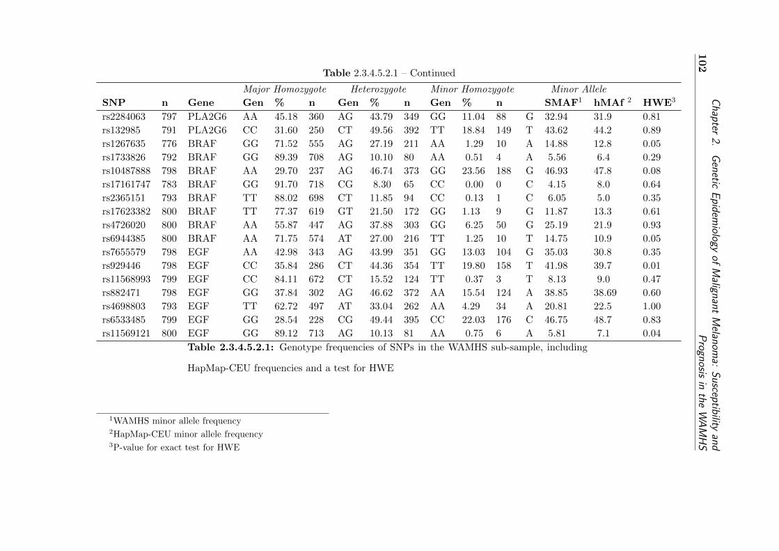
102
Chapter
2.G
eneticE
pidemiology
ofM
alignantM
elanoma:
Susceptibility
andP
rognosisin
theW
AM
HS
Table 2.3.4.5.2.1 – Continued
Major Homozygote Heterozygote Minor Homozygote Minor Allele
SNP n Gene Gen % n Gen % n Gen % n SMAF1 hMAf 2 HWE3
rs2284063 797 PLA2G6 AA 45.18 360 AG 43.79 349 GG 11.04 88 G 32.94 31.9 0.81
rs132985 791 PLA2G6 CC 31.60 250 CT 49.56 392 TT 18.84 149 T 43.62 44.2 0.89
rs1267635 776 BRAF GG 71.52 555 AG 27.19 211 AA 1.29 10 A 14.88 12.8 0.05
rs1733826 792 BRAF GG 89.39 708 AG 10.10 80 AA 0.51 4 A 5.56 6.4 0.29
rs10487888 798 BRAF AA 29.70 237 AG 46.74 373 GG 23.56 188 G 46.93 47.8 0.08
rs17161747 783 BRAF GG 91.70 718 CG 8.30 65 CC 0.00 0 C 4.15 8.0 0.64
rs2365151 793 BRAF TT 88.02 698 CT 11.85 94 CC 0.13 1 C 6.05 5.0 0.35
rs17623382 800 BRAF TT 77.37 619 GT 21.50 172 GG 1.13 9 G 11.87 13.3 0.61
rs4726020 800 BRAF AA 55.87 447 AG 37.88 303 GG 6.25 50 G 25.19 21.9 0.93
rs6944385 800 BRAF AA 71.75 574 AT 27.00 216 TT 1.25 10 T 14.75 10.9 0.05
rs7655579 798 EGF AA 42.98 343 AG 43.99 351 GG 13.03 104 G 35.03 30.8 0.35
rs929446 798 EGF CC 35.84 286 CT 44.36 354 TT 19.80 158 T 41.98 39.7 0.01
rs11568993 799 EGF CC 84.11 672 CT 15.52 124 TT 0.37 3 T 8.13 9.0 0.47
rs882471 798 EGF GG 37.84 302 AG 46.62 372 AA 15.54 124 A 38.85 38.69 0.60
rs4698803 793 EGF TT 62.72 497 AT 33.04 262 AA 4.29 34 A 20.81 22.5 1.00
rs6533485 799 EGF GG 28.54 228 CG 49.44 395 CC 22.03 176 C 46.75 48.7 0.83
rs11569121 800 EGF GG 89.12 713 AG 10.13 81 AA 0.75 6 A 5.81 7.1 0.04
Table 2.3.4.5.2.1: Genotype frequencies of SNPs in the WAMHS sub-sample, including
HapMap-CEU frequencies and a test for HWE
1WAMHS minor allele frequency2HapMap-CEU minor allele frequency3P-value for exact test for HWE

2.3. The Western Australian Melanoma Health Study 103
2.3.4.6 Generalisation of sub-sample to population and participating
cases
2.3.4.6.1 Introduction
It is important that, as much as possible, a selected sub-sample represents the
eligible population and the participating cases so that results can be generalised
back to the participating sample, and in turn, the whole eligible population. The
eligible population in this thesis were all adult invasive cases of melanoma which
were diagnosed between January 2006 and September 2009 and were notified to
the WACR. WAMHS participating cases were all subjects who consented to par-
ticipate in the WAMHS, and who fully or partly completed questionnaires and/or
provided blood samples for DNA in either the pilot or the full-launch studies.
Subjects were included in the sub-sample on the basis that they had a recorded
Breslow thickness, therefore the eligible population and WAMHS participating
cases sample include only those subjects with a Breslow thickness recorded.
2.3.4.6.2 Methods
Comparisons between the selected sub-sample and both the WAMHS cases and
the eligible population were calculated for Breslow thickness, sex, age at diagnosis,
melanoma site and Clark’s level distributions. Differences in mean logged Breslow
thickness between the sub-sample and two other samples was calculated by a one-
sample t-test, with the null hypothesis that the sub-sample mean was equal to
both the WAMHS participating cases mean and population mean. Differences in
sex, age at diagnosis, Clark’s level and melanoma site distributions were calculated
using Fisher’s exact tests on contingency tables.

104Chapter 2. Genetic Epidemiology of Malignant Melanoma: Susceptibility and
Prognosis in the WAMHS
2.3.4.6.3 Results
Differences in Breslow thickness, sex, age at diagnosis, Clark’s level and melanoma
site distributions are shown in Table 2.3.4.6.3.1. The eligible population consisted
of 3,284 individuals who were eligible for inclusion in the WAMHS. The participat-
ing cases consisted of 1,418 individuals, and is a subset of the eligible population.
The sub-sample of 800 Caucasian subjects used in this thesis is a subset of the
WAMHS participating cases sample.
No significant differences were detected between the sub-sample used in this thesis
and the WAMHS case sample. This indicates that the sample of 800 subjects used
in this thesis is representative of the sample of 1,418 subjects who participated in
the WAMHS.
There were no significant differences in Breslow thickness, Clark’s level or melanoma
site between the WAMHS sub-sample used in this thesis and the eligible popula-
tion, with Fisher p-values of 0.75, 0.95 and 0.76, respectively.
Significant differences were observed between the distributions of sex (P=0.02)
and age (P<0.001). There was a higher proportion of females represented in the
WAMHS sub-sample compared to the eligible population, with females account-
ing for 43.88% (n=351) of the sample and only 39.37% (n=1,293) of the eligible
population. There was a higher proportion of individuals aged between 60 and
74 at the time of melanoma diagnosis in the WAMHS sub-sample, and a lower
proportion of all other age groups in the WAMHS sub-sample.

2.3. The Western Australian Melanoma Health Study 105
These differences in sex and age at diagnosis means that the WAMHS sub-sample
may not be representative of the eligible population.

106
Chapter
2.G
eneticE
pidemiology
ofM
alignantM
elanoma:
Susceptibility
andP
rognosisin
theW
AM
HS
VariableSub–sample WAMHS cases p-value Eligible Population p-value
(n=800) (n=1,418) (n=3,284)
Continuous variable, geometric mean (95% CI)
Breslow thickness, mm 0.73 (0.69, 0.77) 0.70 (0.67, 0.73) 0.24 0.73 (0.71, 0.75) 0.75
Dichotomous and categorical variables, % [n]
Sex
Male 56.12 [449] 58.89 [835] 60.60 [1991]
Female 43.88 [351] 41.11 [583] 0.22 39.37 [1293] 0.02
Age at diagnosis
18–29 1.38 [11] 2.05 [29] 3.87 [127]
30–44 12.13 [97] 13.61 [193] 15.99 [525]
45–59 30.37 [243] 32.79 [465] 0.28 31.18 [1024] <0.001
60–74 45.25 [362] 41.11 [583] 36.87 [1211]
75–80 10.87 [87] 10.44 [148] 12.09 [397]
Clark’s Level
II 36.25 [290] 37.73 [535] 37.42 [1229]
III 26.00 [208] 26.16 [371] 25.12 [825]
IV 33.88 [271] 32.93 [467] 0.28 33.43 [1098] 0.95
V 2.75 [22] 2.40 [34] 2.98 [98]
Unknown 1.12 [9] 0.78 [11] 0.12 [34]
Melanoma Site
Head and neck 17.00 [136] 15.73 [223] 16.60 [545]
Trunk 38.25 [306] 38.36 [544] 38.61 [1268]
Upper limb 23.37 [187] 23.70 [336] 0.79 23.54 [773] 0.76
Lower limb 21.38 [171] 22.00 [312] 20.98 [89]
Unknown 0.00 [0] 0.21 [3] 0.27 [9]
Table 2.3.4.6.3.1: Comparisons between the WAMHS sub-sample (n=800), WAMHS participating cases (n=1,418), and the
eligible population (n=3,284)

2.3. The Western Australian Melanoma Health Study 107
2.3.5 Summary
In this section, the establishment of the WAMHS resource has been described,
including the pilot study and full-scale launch of the study. Analysis of comple-
tion rates revealed that the completion rates of study components increased after
changes to the study protocol. Analysis of consenting, non-consenting and non-
responding subjects found that consenting and non-consenting subjects differed
in their age of diagnosis, while consenting and non-responding subjects differed in
both their age of diagnosis and sex.
Eligible subjects were identified through the WACR. Initially, each subject’s doc-
tor was contacted regarding their patient’s suitability to be contacted about the
study. If deemed suitable, subjects were subsequently contacted. This method
had both its benefits and limitations. Contacting the subject’s doctor initially
allowed the doctor to indicate whether their patient was suitable to be contacted
about participation in the study. Possible reasons not to contact their patient
included an inability to speak English, or the presence of co-morbidities which
meant contact or participation in the study was not suitable. Therefore, it is pos-
sible that the WAMHS sample has less non-English-speaking participants than
in the entire eligible population. There is also a possibility that individuals with
co-morbidities, such as dementia, or advanced melanoma were not invited to par-
ticipate in the study after their doctor deemed them not suitable to be contacted.
However, potential biases are likely to be small, as out of the 3,347 doctor contacts,
only 3% (n=112) of patients were not suitable to be contacted regarding the study.
Aside from these possible biases, one benefit of the study recruitment is that there

108Chapter 2. Genetic Epidemiology of Malignant Melanoma: Susceptibility and
Prognosis in the WAMHS
was limited selection bias when subjects were first identified through the WACR.
This meant that individuals contacted should have been representative of the en-
tire eligible population, and should not have differed in terms of demographic or
phenotypic variables. If recruiting subjects through a clinic, many selection biases
are possible, for example, it is possible that only subjects who live within a set
geographical distance from the clinic may be approached about participating in
the study. However, recruitment through the WACR meant that the WAMHS
was able to contact subjects from all over Western Australia, such that rural and
urban areas should be evenly represented. Also, as blood donation was possible
at many PathWest locations throughout Western Australia, there should not have
been an over-representation of any such geographical area. Analyses (not shown)
found that 70% of WAMHS subjects lived in urban areas, and 30% lived in rural
areas. These rates are comparable with the state geographical distributions, of
74% urban, and 26% rural [173].
Descriptive analyses of study variables identified several key variables which dif-
fered between sexes, including age at diagnosis, site, and pigmentation traits. The
WAMHS sub-sample used in this thesis was also described, with descriptive anal-
yses of phenotypic and genotypic variables performed.
Five of the 42 genotyped SNPs were not in HWE. These SNPs were IRF4 rs12203592,
BRAF rs12676365, BRAF rs6944385, EGF rs929446 and EGF rs11569121. Depar-
tures from HWE may be explained by genotyping errors, selection bias, violation
of the underlying assumptions, or chance [30]. However, departures from HWE
in cases does not necessarily represent a flawed study. Instead, departures from
HWE in cases may indicate an association between these SNPs and melanoma. In
2.3. The Western Australian Melanoma Health Study 109
fact, it has been proposed that deviations from HWE can be used as a screening
process to detect gene-disease associations [174].
Qualitative analysis of the key variables available from the WACR and the WAMHS
sub-sample – Breslow thickness, Clark’s level, age at diagnosis, sex and melanoma
site – revealed that Breslow thickness, Clark’s level, and site were similar between
the sub-sample used in this thesis and the eligible population for this thesis (sub-
jects with a recorded Breslow thickness).
The sub-sample of 800 subjects used in this thesis were the first 800 Caucasian
subjects with a recorded Breslow thickness who completed their questionnaire and
blood sample before November 2009. Therefore, there is a potential that these
early-responders may not have been similar to the late-responders. However, com-
parisons between the sub-sample and the WAMHS cases who participated in at
least one component of the study did not detect any significant differences between
these two samples for Breslow thickness, sex, age, Clark’s level and melanoma site.
In addition, the inclusion of only live subjects into the study may introduce bias.
Deceased subjects may have been different compared to live subjects, in particular
for characteristics which may have affected mortality, such as Breslow thickness.
However, this is not likely to have impacted greatly on the analyses as only 118
out of 3,420 (3.45%) individuals died prior to contact.
The sex distribution was skewed, with approximately 56% of the sub-sample male.
This a lower than expected number, given that it is expected that males are ap-
110Chapter 2. Genetic Epidemiology of Malignant Melanoma: Susceptibility and
Prognosis in the WAMHS
proximately 1.5 times more likely to be diagnosed with melanoma [63]. Therefore,
approximately 60% of the sub-sample would be expected to be male. In fact, anal-
ysis of the entire population diagnosed with melanoma in the diagnosis time frame
(n=3,284) revealed that 60.60% were male. The sex distribution of the eligible
population and the sub-sample used in this thesis differed, with 61% of the eligi-
ble population male, compared to only 56% males in the sub-sample. This may
indicate that women were more likely to participate in the study, or were more
likely to be early-responders, and therefore included in the sub-sample for this
thesis.
Age at diagnosis also differed between the sub-sample used in this thesis and the
eligible population. There was a higher proportion of individuals aged between 60
and 74 years in the sub-sample, and a lower proportion of individuals in all other
age groups. This may indicate that individuals aged between 60 and 74 were more
likely to participate in the study, or be early-responders.
With the exception of sex and age, analyses revealed that the WAMHS sub-
sample used in this thesis was generally representative of the eligible population.
Therefore, analyses which follow in the following sections should be generalisable
back to the entire melanoma population. These results may not be generalisable
if they are sex- or age-specific association results.

2.4. Association of Candidate Loci with Melanoma Susceptibility 111
2.4 Association of Candidate Loci with Melanoma Susceptibility
2.4.1 Introduction
The aim of this section is to investigate the genetic association of 42 candidate
SNPs in 16 candidate loci with melanoma risk using WAMHS cases and relevant
controls. The 42 genotyped SNPs described in Section 2.3.4.2 were chosen as they
had been identified as melanoma-risk SNPs, therefore replication of their associa-
tions with melanoma-risk in the WAMHS sample was investigated. Although not
a primary aim of this thesis, this was thought to be important to inform both
the generalisability of the WAMHS genetic association results and the interpre-
tation of any genetic associations with melanoma prognostic phenotypes. In this
section, SNP allelic frequencies in WAMHS cases were compared to two general
population (unselected) control samples: the Busselton Health Study (BHS) and
HapMap-CEU populations. The results of these analyses are then presented and
discussed.
2.4.2 Methods
2.4.2.1 Study populations
Data from two independent populations, one from the United States of America,
and one from Western Australia, were used to investigate the role of candidate
SNPs with melanoma risk.
The WAMHS sample (i.e. cases) used in these analyses was the sub-sample of 800
Caucasian individuals described earlier in Section 2.3.4.

112Chapter 2. Genetic Epidemiology of Malignant Melanoma: Susceptibility and
Prognosis in the WAMHS
The two non-melanoma populations (i.e. controls) were the HapMap-CEU and
the BHS populations. HapMap-CEU is a population of Caucasian individuals
from Utah in the United States of America, with Northern and Western Euro-
pean ancestry [175]. HapMap tag-SNPs have been shown to perform well in the
Australian population [176]. The HapMap-CEU sample size differs depending on
which SNPs are examined. For the SNPs investigated in this thesis, the HapMap
sample size ranged from 55 to 113 individuals. No phenotypic data, including age
or sex, were available for these individuals.
The BHS is a longitudinal epidemiological study of participants residing in Bus-
selton, a coastal town in the south-west of Western Australia. Since 1966, a series
of health surveys has collected epidemiological data on over 16,000 men, women
and children [177, 178]. For the current study, genotypic data from a GWAS un-
dertaken using the Illumina 610-Quad BeadChip was used. Phenotypic data was
collected as part of the 1994-1995 collection period. The BHS sample used in this
thesis consisted of 1,366 unrelated individuals, however not all individuals were
successfully genotyped at each SNP. For the SNPs investigated in this thesis, the
BHS sample size ranged from 1,322 to 1,366 individuals
Table 2.4.2.1.1 shows some characteristics of the BHS sample used in this thesis.
The sample consisted of 57.98% females and the median age of the sample was
53.05 years.

2.4. Association of Candidate Loci with Melanoma Susceptibility 113
VariableBHS Sample
(n=1,366)
Continuous variables, median (IQR)
Age at data collection, years 53.05 (28.1)
BMI, kg/m2 25.97 (5.12)
Dichotomous variable, % [n]
Sex
Male 42.02 [574]
Female 57.98 [792]
Table 2.4.2.1.1: Participant characteristics of the BHS sample
2.4.2.2 Statistical methods
Genotype frequency distributions were compared between the WAMHS sample
and Hapmap-CEU frequencies using Fisher’s exact test for contingency tables.
As additional covariate data were available in the BHS sample, multivariate case-
control analyses were undertaken for the WAMHS-BHS comparisons. WAMHS
genotype frequency distributions were compared to BHS genotype frequencies
using a generalised linear model, adjusted for any covariates common to both data
sets and significantly associated (P< 0.05) with melanoma risk. P-values were
presented as Likelihood Ratio Test (LRT) p-values. The LRT-statistic, D, was
calculated by D = −2 loge(likelihood [pheno]) − 2 loge(likelihood [pheno+SNP]),
where the model ‘pheno’ contains only the significant phenotypic variables and the
‘pheno+SNP’ model contains both phenotypic variables and the SNP. D is then
compared to a Chi-squared distribution with df1-df2 degrees of freedom, where
df1 and df2 are the degrees of freedom for the ‘pheno’ and ‘pheno+SNP’ models
respectively.

114Chapter 2. Genetic Epidemiology of Malignant Melanoma: Susceptibility and
Prognosis in the WAMHS
2.4.3 Results
Genotype frequency distributions between the WAMHS sample and HapMap-
CEU and BHS are presented in Table 2.4.3.1. Two SNPs, OCA2 rs1800401 and
TPCN2 rs35264875, were not genotyped in either the HapMap-CEU or the BHS
samples, and are therefore not shown in the table.
Genotype distributions were available for 40 of the 42 SNPs in the HapMap-CEU
sample. Statistical analysis revealed that seven genotypic distributions were sta-
tistically different from the HapMap genotypic distributions at the 5% level of sig-
nificance (MC1R rs3212363, TYR rs1042602, TYR rs1393350, KITLG rs12821256,
SLC2A4 rs12896399, IRF4 rs12203592, BRAF rs17161747), indicating their pos-
sible role as melanoma-risk SNPs. Three genotypic distributions showed marginal
significance (MYH7B rs1885120, MC1R rs1805005, MTAP rs1011970). When ad-
justed for multiple testing using FDR, no SNPs were significantly associated with
melanoma-risk compared to the HapMap-CEU sample.
Twenty seven of the 48 SNPs were available as genotyped or imputed SNPs in the
BHS GWAS. Multivariate modelling between WAMHS cases and BHS controls
found that the phenotypes sex, BMI, age, age2, age3 and an age:sex interaction
were significantly associated with melanoma-risk (Table 2.4.3.2).
After adjustment for these phenotypic variables, comparison of genotypic dis-
tributions between the WAMHS cases and BHS controls found nine distribu-
tions which were statistically different at the 5% level of significance (CDC91L1
rs910873, MC1R rs258322, TYR rs1393350, HERC2 12913832, IRF4 rs12203592

2.4. Association of Candidate Loci with Melanoma Susceptibility 115
MTAP rs4636294, MTAP rs7023329, MTAP rs1011970, BRAF rs6944385). In ad-
dition, five genotypic distributions were marginally significant (P<0.10), MYH7B
rs1885120, MTAP rs10757257, PLA2G6 rs2284063, PLA2G6 rs132985, BRAF
rs10487888). After adjustment for multiple testing, six SNP associations us-
ing the BHS sample remained significant with q-values < 0.05 (MC1R rs258322,
TYR rs1393350, IRF4 rs12203592, MTAP rs7023329, MTAP rs1011970, BRAF
rs6944385).
At the 5% level of significance, two SNPs, TYR rs1393350 and IRF4 rs12203592,
were both significantly associated with melanoma risk compared to both the
HapMap-CEU and BHS populations. However, after adjustment for multiple
testing, no SNPs were significantly associated with melanoma risk across both
populations.
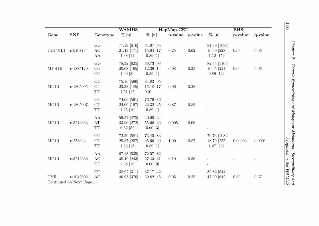
116
Chapter
2.G
eneticE
pidemiology
ofM
alignantM
elanoma:
Susceptibility
andP
rognosisin
theW
AM
HS
WAMHS HapMap-CEU BHSGene SNP Genotype % [n] % [n] p-value q-value % [n] p-value1 q-value
GG 77.19 [616] 84.07 [95] 81.89 [1099]CDC91L1 rs910873 AG 21.43 [171] 15.04 [17] 0.25 0.62 16.99 [228] 0.05 0.06
AA 1.38 [11] 0.89 [1] 1.12 [15]
GG 78.32 [625] 86.73 [98] 82.45 [1109]MYH7B rs1885120 CG 20.68 [165] 12.39 [14] 0.08 0.35 16.65 [224] 0.06 0.06
CC 1.00 [8] 0.89 [1] 0.89 [12]
GG 75.16 [596] 84.82 [95] -MC1R rs1805005 GT 23.33 [185] 15.18 [17] 0.06 0.28 - - -
TT 1.51 [12] 0 [0] -
CC 74.06 [591] 76.79 [86] -MC1R rs1805007 CT 24.69 [197] 22.32 [25] 0.87 0.85 - - -
TT 1.25 [10] 0.89 [1] -
AA 59.52 [475] 40.00 [24] -MC1R rs3212363 AT 33.96 [272] 55.00 [33] 0.005 0.06 - - -
TT 6.52 [52] 5.00 [3] -
CC 72.50 [581] 73.45 [83] 79.73 [1082]MC1R rs258322 CT 25.87 [207] 25.66 [29] 1.00 0.87 18.79 [255] 0.00003 0.0001
TT 1.63 [13] 0.89 [1] 1.47 [20]
AA 67.13 [535] 72.57 [82] -MC1R rs3212369 AG 30.49 [243] 27.43 [31] 0.19 0.56 - - -
GG 2.38 [19] 0.00 [0] -
CC 38.92 [311] 37.17 [42] 39.82 [544]TYR rs1042602 AC 46.93 [376] 39.82 [45] 0.05 0.25 47.00 [642] 0.80 0.37Continued on Next Page. . .

2.4.A
ssociation
ofC
andidateL
oci
with
Melanom
aS
usceptibility117
Table 2.4.3.1 - Continued
WAMHS HapMap BHSGene SNP Genotype % [n] % [n] p-value q-value % [n] p-value1 q-value
AA 14.15 [113] 23.01 [26] 13.18 [180]
GG 47.55 [379] 62.83 [71] 52.12 [689]TYR rs1393350 AG 40.65 [324] 29.20 [33] 0.01 0.07 40.32 [533] 0.003 0.01
AA 11.79 [94] 7.97 [9] 7.56 [100]
CC 48.80 [387] 47.79 [54] 47.84 [653]TYRP1 rs1408799 CT 41.87 [332] 43.36 [49] 0.97 0.86 41.25 [563] 0.83 0.38
TT 9.33 [74] 8.85 [10] 10.92 [149]
TT 80.98 [647] 71.68 [81] 77.58 [1059]SLC24A4 rs12821256 CT 18.02 [144] 27.43 [31] 0.05 0.25 20.59 [281] 0.14 0.10
CC 1.00 [8] 0.89 [1] 1.83 [25]
GG 28.54 [228] 16.81 [19] 30.31 [414]KITLG rs12896399 GT 51.69 [413] 52.22 [59] 0.004 0.06 49.41 [675] 0.22 0.14
TT 19.77 [158] 30.97 [35] 20.28 [277]
AA 32.29 [258] 27.03 [111] -IRF4 rs1540771 AG 49.56 [396] 57.66 [64] 0.30 0.66 - - -
GG 18.15 [145] 15.31 [17] -
GG 36.64 [292] 32.74 [37] 35.16 [480]TPCN2 rs3829241 AG 45.92 [366] 49.56 [56] 0.71 0.82 49.45 [675] 0.37 0.21
AA 17.44 [139] 17.70 [20] 15.38 [210]
GG 80.10 [632] 85.72 [96] -OCA2 rs1800407 AG 18.76 [148] 13.39 [15] 0.35 0.70 - - -
AA 1.14 [9] 0.89 [1] -
Continued on Next Page. . .
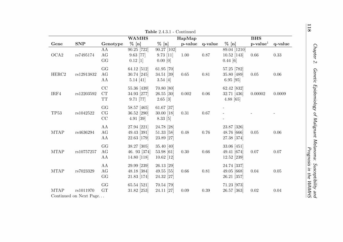
118
Chapter
2.G
eneticE
pidemiology
ofM
alignantM
elanoma:
Susceptibility
andP
rognosisin
theW
AM
HS
Table 2.4.3.1 - Continued
WAMHS HapMap BHSGene SNP Genotype % [n] % [n] p-value q-value % [n] p-value1 q-value
AA 90.25 [722] 90.27 [102] 89.04 [1210]OCA2 rs7495174 AG 9.63 [77] 9.73 [11] 1.00 0.87 10.52 [143] 0.66 0.33
GG 0.12 [1] 0.00 [0] 0.44 [6]
GG 64.12 [512] 61.95 [70] 57.25 [782]HERC2 rs12913832 AG 30.74 [245] 34.51 [39] 0.65 0.81 35.80 [489] 0.05 0.06
AA 5.14 [41] 3.54 [4] 6.95 [95]
CC 55.36 [439] 70.80 [80] 62.42 [832]IRF4 rs12203592 CT 34.93 [277] 26.55 [30] 0.002 0.06 32.71 [436] 0.00002 0.0009
TT 9.71 [77] 2.65 [3] 4.88 [65]
GG 58.57 [465] 61.67 [37] -TP53 rs1042522 CG 36.52 [290] 30.00 [18] 0.31 0.67 - - -
CC 4.91 [39] 8.33 [5] -
AA 27.94 [221] 24.78 [28] 23.87 [326]MTAP rs4636294 AG 49.43 [391] 51.33 [58] 0.48 0.76 48.76 [666] 0.05 0.06
AA 22.63 [179] 23.89 [27] 27.38 [374]
GG 38.27 [305] 35.40 [40] 33.06 [451]MTAP rs10757257 AG 46. 93 [374] 53.98 [61] 0.30 0.66 49.41 [674] 0.07 0.07
AA 14.80 [118] 10.62 [12] 12.52 [239]
AA 29.99 [239] 26.13 [29] 24.74 [337]MTAP rs7023329 AG 48.18 [384] 49.55 [55] 0.66 0.81 49.05 [668] 0.04 0.05
GG 21.83 [174] 24.32 [27] 26.21 [357]
GG 65.54 [521] 70.54 [79] 71.23 [973]MTAP rs1011970 GT 31.82 [253] 24.11 [27] 0.09 0.39 26.57 [363] 0.02 0.04Continued on Next Page. . .

2.4.A
ssociation
ofC
andidateL
oci
with
Melanom
aS
usceptibility119
Table 2.4.3.1 - Continued
WAMHS HapMap BHSGene SNP Genotype % [n] % [n] p-value q-value % [n] p-value1 q-value
TT 2.64 [21] 5.35 [6] 2.20 [30]
AA 45.18 [360] 46.02 [52] 40.26 [550]PLA2G6 rs2284063 AG 43.79 [349] 44.25 [50] 0.96 0.86 46.49 [635] 0.09 0.07
GG 11.04 [88] 9.73 [11] 13.25 [181]
CC 31.60 [250] 30.09 [34] 27.11 [370]PLA2G6 rs132985 CT 49.56 [392] 51.33 [58] 0.95 0.86 50.04 [683] 0.09 0.07
TT 18.84 [149] 18.58 [21] 22.86 [312]
GG 71.52 [555] 76.11 [86] 75.11 [1026]BRAF rs1267635 AG 27.19 [211] 22.12[25] 0.44 0.74 22.99 [314] 0.19 0.13
AA 1.29 [10] 1.77 [2] 1.90 [26]
GG 89.39 [708] 87.27 [96] -BRAF rs1733826 AG 10.10 [80] 12.73 [14] 0.65 0.81 - - -
AA 0.51 [4] 0.00 [0] -
AA 29.70 [237] 23.89 [27] 31.77[434]BRAF rs10487888 AG 46.74 [373] 56.64 [64] 0.16 0.51 49.27 [673] 0.07 0.07
GG 23.56 [188] 19.47 [22] 18.96 [259]
GG 91.70 [718] 84.07 [95] -BRAF rs17161747 CG 8.30 [66] 15.93 [18] 0.01 0.70 - - -
CC 0.00 [0] 0.00 [0] -
TT 88.02 [698] 90.00 [54] -BRAF rs2365151 CT 11.85 [94] 10.00 [6] 0.85 0.85 - - -
CC 0.13 [1] 0.00 [0] -
Continued on Next Page. . .
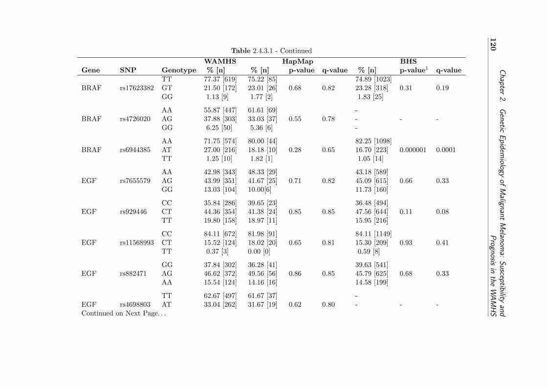
120
Chapter
2.G
eneticE
pidemiology
ofM
alignantM
elanoma:
Susceptibility
andP
rognosisin
theW
AM
HS
Table 2.4.3.1 - Continued
WAMHS HapMap BHSGene SNP Genotype % [n] % [n] p-value q-value % [n] p-value1 q-value
TT 77.37 [619] 75.22 [85] 74.89 [1023]BRAF rs17623382 GT 21.50 [172] 23.01 [26] 0.68 0.82 23.28 [318] 0.31 0.19
GG 1.13 [9] 1.77 [2] 1.83 [25]
AA 55.87 [447] 61.61 [69] -BRAF rs4726020 AG 37.88 [303] 33.03 [37] 0.55 0.78 - - -
GG 6.25 [50] 5.36 [6] -
AA 71.75 [574] 80.00 [44] 82.25 [1098]BRAF rs6944385 AT 27.00 [216] 18.18 [10] 0.28 0.65 16.70 [223] 0.000001 0.0001
TT 1.25 [10] 1.82 [1] 1.05 [14]
AA 42.98 [343] 48.33 [29] 43.18 [589]EGF rs7655579 AG 43.99 [351] 41.67 [25] 0.71 0.82 45.09 [615] 0.66 0.33
GG 13.03 [104] 10.00[6] 11.73 [160]
CC 35.84 [286] 39.65 [23] 36.48 [494]EGF rs929446 CT 44.36 [354] 41.38 [24] 0.85 0.85 47.56 [644] 0.11 0.08
TT 19.80 [158] 18.97 [11] 15.95 [216]
CC 84.11 [672] 81.98 [91] 84.11 [1149]EGF rs11568993 CT 15.52 [124] 18.02 [20] 0.65 0.81 15.30 [209] 0.93 0.41
TT 0.37 [3] 0.00 [0] 0.59 [8]
GG 37.84 [302] 36.28 [41] 39.63 [541]EGF rs882471 AG 46.62 [372] 49.56 [56] 0.86 0.85 45.79 [625] 0.68 0.33
AA 15.54 [124] 14.16 [16] 14.58 [199]
TT 62.67 [497] 61.67 [37] -EGF rs4698803 AT 33.04 [262] 31.67 [19] 0.62 0.80 - - -Continued on Next Page. . .
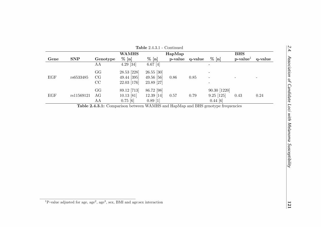
2.4.A
ssociation
ofC
andidateL
oci
with
Melanom
aS
usceptibility121
Table 2.4.3.1 - Continued
WAMHS HapMap BHSGene SNP Genotype % [n] % [n] p-value q-value % [n] p-value1 q-value
AA 4.29 [34] 6.67 [4] -
GG 28.53 [228] 26.55 [30] -EGF rs6533485 CG 49.44 [395] 49.56 [56] 0.86 0.85 - - -
CC 22.03 [176] 23.89 [27] -
GG 89.12 [713] 86.72 [98] 90.30 [1220]EGF rs11569121 AG 10.13 [81] 12.39 [14] 0.57 0.79 9.25 [125] 0.43 0.24
AA 0.75 [6] 0.89 [1] 0.44 [6]
Table 2.4.3.1: Comparison between WAMHS and HapMap and BHS genotype frequencies
1P-value adjusted for age, age2, age3, sex, BMI and age:sex interaction
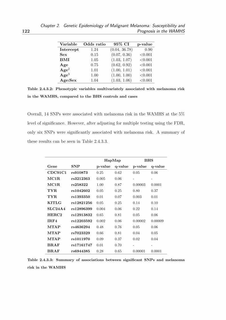
122Chapter 2. Genetic Epidemiology of Malignant Melanoma: Susceptibility and
Prognosis in the WAMHS
Variable Odds ratio 95% CI p-value
Intercept 1.24 (0.04, 36.78) 0.90Sex 0.15 (0.07, 0.36) <0.001BMI 1.05 (1.03, 1.07) <0.001Age 0.75 (0.62, 0.92) <0.001Age2 1.01 (1.00, 1.01) <0.001Age3 1.00 (1.00, 1.00) <0.001Age:Sex 1.04 (1.03, 1.06) <0.001
Table 2.4.3.2: Phenotypic variables multivariately associated with melanoma risk
in the WAMHS, compared to the BHS controls and cases
Overall, 14 SNPs were associated with melanoma risk in the WAMHS at the 5%
level of significance. However, after adjusting for multiple testing using the FDR,
only six SNPs were significantly associated with melanoma risk. A summary of
these results can be seen in Table 2.4.3.3.
HapMap BHS
Gene SNP p-value q-value p-value q-value
CDC91C1 rs910873 0.25 0.62 0.05 0.06
MC1R rs3212363 0.005 0.06 - -
MC1R rs258322 1.00 0.87 0.00003 0.0001
TYR rs1042602 0.05 0.25 0.80 0.37
TYR rs1393350 0.01 0.07 0.003 0.01
KITLG rs12821256 0.05 0.25 0.14 0.10
SLC24A4 rs12896399 0.004 0.06 0.22 0.14
HERC2 rs12913832 0.65 0.81 0.05 0.06
IRF4 rs12203592 0.002 0.06 0.00002 0.00009
MTAP rs4636294 0.48 0.76 0.05 0.06
MTAP rs7023329 0.66 0.81 0.04 0.05
MTAP rs1011970 0.09 0.37 0.02 0.04
BRAF rs17161747 0.01 0.70 - -
BRAF rs6944385 0.28 0.65 0.00001 0.0001
Table 2.4.3.3: Summary of associations between significant SNPs and melanoma
risk in the WAMHS

2.4. Association of Candidate Loci with Melanoma Susceptibility 123
2.4.3.1 Summary of results
Seven SNPs (from six genes) were associated with melanoma risk when com-
pared to HapMap-CEU, and nine SNPs (from seven genes) were associated with
melanoma risk when compared to the BHS controls. Only two SNPs were sig-
nificantly associated with melanoma risk across both HapMap-CEU and BHS
samples. After adjustment for multiple testing, no SNPs were significantly asso-
ciated with melanoma risk when compared to the HapMap-CEU, and six SNPS
(from five genes) were significantly associated with melanoma risk compared to
the BHS controls. It is likely that the results using the BHS sample are more
reliable than those using the HapMap-CEU sample, as the BHS sample is larger,
and is also sampled from a Western Australian population. The significant gene
and SNP associations, both before and after adjustments for multiple testing, are
described below.
2.4.3.1.1 MTAP
Compared to the BHS controls, three SNPs in the MTAP gene were signifi-
cantly associated with melanoma risk - rs4636294, rs7023329 and rs1011970. The
melanoma-risk alleles for these SNPs were consistent with the melanoma-risk SNP
alleles identified in previous studies. In particular, the rare variants of rs4636294
and rs7023329 were both associated with increased melanoma risk and increased
naevi count in GWAS by Falchi et al. [105] and Bishop et al. [106], while the
rare variant of the rs1011970 SNP was associated with naevi count only [105].
The fourth MTAP SNP genotyped, rs10757257, which had been identified as a
melanoma risk and naevi count SNP [105, 106] was marginally associated with
melanoma risk, with a p-value of 0.07.

124Chapter 2. Genetic Epidemiology of Malignant Melanoma: Susceptibility and
Prognosis in the WAMHS
After adjusting for multiple testing, the associations between melanoma risk and
rs7023329 (q=0.05) and rs1011970 (q=0.04) remained significant.
Compared to the HapMap-CEU sample, no MTAP SNPs were significantly asso-
ciated with melanoma risk in this study.
2.4.3.1.2 CDC91C1
The rs910873 SNP in the CDC91C1 gene was significantly associated with melanoma
risk when compared to the BHS controls. In particular, the ‘A’ variant of this SNP
was associated with melanoma risk in this study. A similar association between
this variant and melanoma risk was also observed in the two GWAS studies by
Brown et al. [107] and Bishop et al. [106]. Compared to the HapMap sample, this
SNP was not associated with melanoma risk. However, the frequency of the ‘G’
allele in the HapMap and BHS samples was substantially lower when compared
to the WAMHS sample. The frequency of the ‘G’ allele in the HapMap and BHS
samples was 8.41% and 9.61% respectively, compared to the WAMHS sample fre-
quency of 12.09%.
After adjusting for multiple testing, the rs910873 SNP was marginally associated
with melanoma risk when compared to the BHS sample (q=0.06).
2.4.3.1.3 TYR
Two SNPs in the TYR gene were associated with melanoma risk in this study.
The ‘A’ variant of the rs1393350 SNP was significantly associated with melanoma

2.4. Association of Candidate Loci with Melanoma Susceptibility 125
risk in this study when compared to the HapMap-CEU and BHS samples. The
genotypic distributions differed greatly between samples, with 63% and 52% of
individuals in the control populations having the common homozygote, compared
to 48% in the WAMHS sample. Similarly, 8% of individuals in the control popu-
lations were rare homozygous, compared to 12% in the WAMHS sample.
This SNP was previously associated with melanoma risk in a study by Bishop et
al. [106]. In addition, the ‘A’ allele was also associated with blonde hair, green
eyes and increased skin sensitivity to the sun in a study by Sulem et al. [109],
which are all known melanoma risk factors.
After adjustment for multiple testing, the rs1393350 SNP remained significantly
associated with melanoma risk when compared to the BHS controls (q=0.01), and
marginally associated (q=0.07) when compared to the HapMap-CEU sample.
The ‘C’ variant of the rs1042602 SNP, also in TYR, was associated with melanoma
risk, compared to the HapMap sample. However, when compared to the BHS con-
trols, the rs1042602 SNP was not associated with melanoma risk, with a p-value
of 0.80. The ‘C’ variant has been associated with melanoma risk in the GWAS by
Bishop et al. [106], and was also associated with freckling in a study by Sulem et
al. [109] which is a known risk factor for melanoma.
After adjustment for multiple testing, the rs1042602 SNP was no longer associated
with melanoma risk when compared to the HapMap sample (q=0.25).

126Chapter 2. Genetic Epidemiology of Malignant Melanoma: Susceptibility and
Prognosis in the WAMHS
2.4.3.1.4 KITLG
The rs12821256 SNP in the KITLG gene was significantly associated with melanoma
risk when compared to the HapMap sample, however no association was detected
between this SNP and melanoma risk using the BHS controls (P=0.14). The ‘T’
variant was associated with melanoma risk in this study, however this association
is in direct contrast to a previous study by Sulem et al. [109]. In the study by
Sulem et al., the ‘C’ variant was associated with blonde hair, which is a melanoma
risk factor, therefore suggesting that the ‘C’ variant is associated with melanoma
risk.
I am unable to explain this difference. However, it may be that the association ob-
served in this study was a false positive, which is supported by the non-significance
of the association when adjusted for multiple testing (q=0.25).
2.4.3.1.5 SLC24A4
The rs12896399 SNP from the SLC24A4 gene was significantly (P=0.05) asso-
ciated with melanoma risk when compared to the HapMap sample, however no
association was detected between this SNP and melanoma risk when compared
to the BHS controls (P=0.22). The ‘G’ variant was associated with melanoma
risk in this study. In a previous study by Sulem et al. [109], the ‘T’ variant was
associated with melanoma risk factors, including blonde hair and increased skin
sensitivity to the sun. The results from the study by Sulem et al. are therefore in
direct contrast from the results of this study.
I am unable to explain this difference. However, as with rs12821256 from KITLG,

2.4. Association of Candidate Loci with Melanoma Susceptibility 127
it may be that the association observed in this study was a false positive. This is
supported by the only marginal significance of the association when adjusted for
multiple testing (q=0.06).
2.4.3.1.6 HERC2
The ‘G’ variant of the rs12913832 SNP in the HERC2 gene was associated with
melanoma risk in this study, when compared to BHS controls. 61.96% of the
WAMHS sample were homozygous for the ‘G’ allele, compared to 57.25% of the
BHS sample. No association was detected between this SNP and melanoma risk
compared to the HapMap sample.
The ‘G’ allele of this SNP has been associated with blue eyes in previous stud-
ies [170,171], and melanoma risk in a recent study by Duffy et al. [179].
After adjustment for multiple testing, the rs12913832 SNP was marginally asso-
ciated with melanoma risk when compared to the BHS controls (q=0.06).
2.4.3.1.7 IRF4
The ‘T’ variant of the rs12203592 SNP in the IRF4 gene was associated with
melanoma risk in this study, compared to both BHS controls and the HapMap
sample. In particular, 71% and 62% of individuals in the control populations had
the common homozygote, compared to 55% in the WAMHS sample. Similarly, 3%
and 5% of individuals in the control populations were rare homozygotes, compared
to 10% in the WAMHS sample. This variant has been found to be associated with
melanoma risk factors, such as blonde hair, lighter skin colour, lighter eye colour

128Chapter 2. Genetic Epidemiology of Malignant Melanoma: Susceptibility and
Prognosis in the WAMHS
and reduced tanning ability in a study by Han et al. [124].
After adjustment for multiple testing, the rs12203592 SNP was marginally associ-
ated with melanoma risk compared to the the HapMap sample (q=0.06), however
this SNP was strongly associated with melanoma risk when using the BHS con-
trols (q=0.0009). HWE analysis from Section 2.3.4.5 revealed that this SNP was
not in HWE in the WAMHS cases, which may have been due to its role as a
melanoma-risk SNP.
The rs1540771 SNP also in the IRF4 gene was not associated with melanoma risk
when compared to the HapMap sample, and this SNP was not available in the
BHS study.
2.4.3.1.8 MC1R
Two SNPS in the MC1R gene were associated with melanoma risk. The rs3212363
SNP was associated with melanoma risk when compared to the HapMap sample,
however this SNP was not available in the BHS sample.
The ‘T ’ variant of the rs258322 SNP was associated with melanoma risk, when
using BHS controls. This variant allele was also identified by Bishop et al. [106]
and Han et al. [124] as a melanoma risk variant. Compared to the HapMap sam-
ple, this SNP was not associated with melanoma risk.
After adjustment for multiple testing, rs3212363 was marginally associated with
melanoma risk compared to the HapMap controls (q=0.06). However, the asso-

2.4. Association of Candidate Loci with Melanoma Susceptibility 129
ciation between rs258322 and melanoma risk was significant when using the BHS
controls (q=0.0001).
2.4.3.1.9 BRAF
Two SNPs on the BRAF gene were significantly associated with melanoma risk.
The ‘G’ variant of the rs17161747 SNP was associated with melanoma risk using
the HapMap sample, however this SNP was not available in the BHS sample. The
rs6944385 SNP was associated with melanoma risk when using the BHS controls,
however there was no association between this SNP and melanoma risk when us-
ing the HapMap sample. HWE analysis from Section 2.3.4.5 revealed that this
SNP was not in HWE in the WAMHS cases, which may have been due to its role
as a melanoma-risk SNP.
After adjustment for multiple testing, both the rs17161747 and the rs6944385
SNPs were no longer associated with melanoma risk when using the HapMap
sample, with q-values of 0.70 and 0.65, respectively. However, when using the
BHS controls, the rs6944385 SNP remained strongly associated with melanoma
risk (q=0.0001).
2.4.3.2 Discussion
The SNPs used in this analysis were chosen as they had been identified as melanoma-
risk SNPs, or were on melanoma candidate genes. This analysis has found 14 SNPs
which were significantly associated with melanoma risk, out of a possible 67 SNP
associations. More specifically, 25 SNPs were not associated with melanoma risk
using either the HapMap sample or BHS controls. These results may be due to a

130Chapter 2. Genetic Epidemiology of Malignant Melanoma: Susceptibility and
Prognosis in the WAMHS
number of reasons which are discussed below.
The WAMHS sample (n=800) is relatively small, and it is likely that the analyses
were underpowered. Similarly, the HapMap sample is small, generally consisting
of approximately 100 individuals. For the rarer SNPs, the rare homozygote count
is very small, often with less than 20 individuals. Therefore, the power to de-
tect differences in genotypic distributions was likely to be low. This was further
evidenced by the substantial differences in genotype distributions between the
WAMHS and the HapMap samples which may have been significant differences if
the HapMap sample size was larger.
In addition, the WAMHS sample did not have many phenotypic variables in com-
mon with both the HapMap and BHS samples. In fact, the HapMap sample did
not contain any phenotypic variables, therefore it was not possible to adjust for
any possible covariates when analysing melanoma risk. There was a limited num-
ber of common phenotypic variables collected as part of the WAMHS and BHS
samples; these were age, sex and BMI. Therefore only these three variables were
considered as covariates. It would be preferable to adjust for more phenotypic
variables, including sun exposure and naevi counts.
There is also a discrepancy between the methods of obtaining the SNP data in
cases and controls. The case (WAMHS) SNPs were all obtained through geno-
typing, while the control SNPs from the BHS consisted of both genotyped and
imputed SNPs. For the imputed SNPs, the program MACH [266] was used to de-
termine the ‘most likely’ genotype for each individual based on a genotype prob-

2.5. Association of Candidate Loci with Breslow thickness 131
ability greater than 0.50. This may have led to biases within the analyses and a
reduction in power, as some genotype uncertainty will remain unaccounted [267].
If possible, it would be preferable to use only genotyped or imputed SNPs in a
case-control study; and if using imputed data, to incorporate the genotype uncer-
tainty into the analysis.
One particular advantage of the BHS sample over the HapMap-CEU sample is
that the BHS individuals are from Western Australia, and are likely to have experi-
enced a similar level of sun exposure, therefore limiting biases due to confounding.
However, the sun exposure or other exposures experienced by the HapMap-CEU
sample are likely to be different to the WAMHS sample.
This is, to the author’s knowledge, the first study which has used Western Aus-
tralian individuals to investigate the role of genetic variants and melanoma risk.
As such, large-scale replication is required in larger Australian samples. This
is particularly relevant for SNPs in MC1R (rs3212363) and BRAF (rs17161747,
rs6944385) which have not been identified previously as melanoma-risk SNPs.
2.5 Association of Candidate Loci with Breslow thickness
2.5.1 Introduction
The aim of the research described in this section was to investigate the associ-
ation between the primary melanoma prognosis phenotype - Breslow thickness
- and genetic variants in candidate genes within the WAMHS population. The
SNPs genotyped (n=42 in 16 genes) were chosen as they had been previously
identified as variants associated with melanoma risk or were from melanoma-risk

132Chapter 2. Genetic Epidemiology of Malignant Melanoma: Susceptibility and
Prognosis in the WAMHS
genes. The associations between these SNPs and melanoma risk in the WAMHS
was reported in Section 2.4 (please see page 111).
In this section, a genetic association study between these SNPs and the best in-
dependent predictor of melanoma prognosis, Breslow thickness, was undertaken.
The results of these genetic association analyses are presented, and their implica-
tions are discussed.
2.5.2 Statistical methods
The methods used for univariate and multivariate association analyses for both
phenotypic and genotypic variables are described in this section. All analyses were
performed in Rv2.10.1. The sub-samples used in these analyses was the WAMHS
sub-sample (n=800) described earlier in Section 2.3.4.
2.5.2.1 Association analyses
2.5.2.1.1 Epidemiological analyses
2.5.2.1.1.1 Univariate analyses
Possible associations were investigated between Breslow thickness and several di-
chotomous, categorical and continuous phenotypic variables, using linear regres-
sion. Due to its skewed distribution, Breslow thickness was transformed using the
formula loge(Breslow thickness) for all analyses. The magnitude of the association
of variables with Breslow thickness were calculated by back-transforming the co-
efficients using the formula 100 ∗ (expcoefficient−1). For continuous phenotypes,
model coefficients were presented as a percentage change for a one unit increase in

2.5. Association of Candidate Loci with Breslow thickness 133
the phenotype. For dichotomous and categorical phenotypes, model coefficients
were presented as a percentage change for each level of the phenotype, compared
to the baseline.
2.5.2.1.1.2 Multivariate analyses
Multivariate models were fitted using generalised linear models (linear regres-
sion) [180]. Independent predictors of Breslow thickness were determined by using
a stepwise variable selection procedure. Starting with the full model of all possible
predictors, a backwards elimination approach was used, based on the Akaike Infor-
mation Criterion (AIC). The AIC attempts to find the model which best explains
the data, while penalising the model for the number of parameters estimated. AIC
is calculated as AIC=2p − 2 loge(L), where p is the number of parameters, and
L is the maximised value of the likelihood function for the estimated model. In
these analyses, the model with the smallest AIC was chosen as the preferred model.
Quadratic effects of age at diagnosis and phenotypic interactions, in particular sex
interactions, were also investigated. Model diagnostic plots, including residual and
Normal quantile-quantile plots were used to check that the final model did not
violate linear regression assumptions.
2.5.2.1.2 Genotypic analyses
2.5.2.1.2.1 Univariate analyses
All 42 SNPs were tested for univariate linear associations with loge(Breslow thick-
ness). These SNPs were tested under a codominant model, with the common ho-
mozygote set as the reference category. A codominant model was chosen initially

134Chapter 2. Genetic Epidemiology of Malignant Melanoma: Susceptibility and
Prognosis in the WAMHS
as inspection of codominant model coefficients can be used to identify the best fit-
ting model (i.e. co-dominant, additive, dominant, or recessive). ANOVA p-values
derived from the F-distribution were used to determine statistical significance,
which was defined at the 5% level of significance.
2.5.2.1.2.2 Multivariate analyses
Multivariate analysis of loge(Breslow thickness) and the 42 SNPs were undertaken.
Each SNP was added to the multivariate phenotypic models derived in Section
2.5.2.1.1.2 (please see page 133). Multivariate analysis was performed to reduce
the variability in the outcome which may enhance the ability to recognize statis-
tically significant effects. Initially each SNP was modelled codominantly. If the
SNP was significantly (P<0.05) or marginally (P<0.10) associated with Breslow
thickness, the model coefficients were investigated to determine if the SNP was
more predictive under either a codominant, additive, dominant or recessive model.
P-values are presented for each genotype factor relative to the baseline (common)
homozygote.
SNP:phenotype interactions were also considered to investigate any non-additive
effect of the SNPs and phenotypes on Breslow thickness. A final model of all
significant SNPs adjusted for significant phenotypes was fitted, including possi-
ble SNP:phenotype interactions. Residual analysis and Normal quantile-quantile
plots were used to check that the final model did not violate linear regression
assumptions.

2.5. Association of Candidate Loci with Breslow thickness 135
2.5.2.2 Statistical power
In statistical analyses, the probability of a ‘false negative’ or Type II error is the
probability of failing to reject the null hypothesis when the null hypothesis is
false. Power is defined as 1 − β, where β is the Type II error rate. Therefore as
the Type II error rate decreases, power increases. Conventionally, power of 0.8 is
considered to be adequate. This means that if 100 tests are performed, when the
null hypothesis is not true, 80 of these tests would reject the null hypothesis and
detect significant differences.
Power in genetic analyses is dependent on the sample size, MAF, size of the
effect and the type of disease model being tested, such as dominant, additive or
recessive. Statistical power was calculated for both genetic main effects and gene-
environment interactions. An alpha level of 0.0012 was used for the genetic main
effects, calculated by 0.0542
. For the interaction effects, 42 x 2 = 84 interaction tests
were performed, and therefore the alpha level used was 0.0006 (0.0584
). In this thesis,
power calculations were performed in the statistical software package Quanto [181]
for a sample size of 800, MAF ranging from 0.1 to 0.5, effect sizes of 0.1, 0.2,
0.3 and 0.5 standard deviations (SD). Main effect power was calculated under
dominant, additive and recessive models. Interaction effect power was calculated
for an additive model, assuming main effects for the gene and environment of
0.5SD, and an environment prevalence of 0.2 and 0.8.
2.5.3 Results
Descriptive statistics for the phenotypic variables and genotyped SNPs were pre-
sented in Section 2.3.4.5 (please see page 91). Results of phenotypic and genotypic
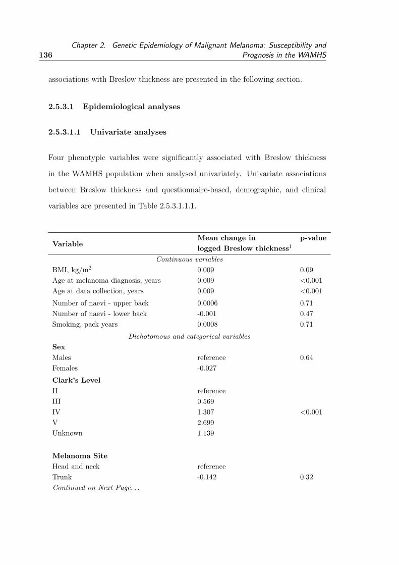
136Chapter 2. Genetic Epidemiology of Malignant Melanoma: Susceptibility and
Prognosis in the WAMHS
associations with Breslow thickness are presented in the following section.
2.5.3.1 Epidemiological analyses
2.5.3.1.1 Univariate analyses
Four phenotypic variables were significantly associated with Breslow thickness
in the WAMHS population when analysed univariately. Univariate associations
between Breslow thickness and questionnaire-based, demographic, and clinical
variables are presented in Table 2.5.3.1.1.1.
VariableMean change in p-value
logged Breslow thickness1
Continuous variables
BMI, kg/m2 0.009 0.09
Age at melanoma diagnosis, years 0.009 <0.001
Age at data collection, years 0.009 <0.001
Number of naevi - upper back 0.0006 0.71
Number of naevi - lower back -0.001 0.47
Smoking, pack years 0.0008 0.71
Dichotomous and categorical variables
Sex
Males reference 0.64
Females -0.027
Clark’s Level
II reference
III 0.569
IV 1.307 <0.001
V 2.699
Unknown 1.139
Melanoma Site
Head and neck reference
Trunk -0.142 0.32
Continued on Next Page. . .

2.5. Association of Candidate Loci with Breslow thickness 137
Table 2.5.3.1.1.1 - Continued
VariableMean change in p-value
logged Breslow thickness1
Upper limb -0.096
Lower limb -0.037
Ever Smoked
No reference
Yes 0.112 0.06
Presence of Naevi
No reference
Yes -0.392 <0.001
Self-reported history of melanoma
No reference
Yes -0.054 0.41
Family history of melanoma
No reference
Yes -0.027 0.69
Skin colour
Very fair reference
Fair -0.021 0.31
Olive/brown 0.155
Hair colour at age 18
Red reference
Fair/blonde -0.119
Light/mouse brown -0.039 0.75
Grey -0.201
Dark brown -0.031
Black -0.149
Eye colour
Blue reference
Grey 0.179
Green 0.089 0.42
Hazel 0.117
Brown 0.035
Sunburn causing blisters, 5-12 years
0 times reference
1-5 times -0.0618
6-10 times -0.029 0.81
Continued on Next Page. . .

138Chapter 2. Genetic Epidemiology of Malignant Melanoma: Susceptibility and
Prognosis in the WAMHS
Table 2.5.3.1.1.1 - Continued
VariableMean change in p-value
logged Breslow thickness1
> 10 times 0.046
Don’t know 0.0607
Sunburn causing blisters, 13-19 years
0 times reference
1-5 times 0.0376
6-10 times -0.090 0.61
> 10 times -0.134
Don’t know 0.067
Sunburn causing blisters, > 20 years
0 times reference
1-5 times -0.014
6-10 times 0.048 0.79
> 10 times 0.186
Don’t know 0.467
Table 2.5.3.1.1.1: Univariate analysis between phenotypic variables with Breslow thick-
ness in the WAMHS
Significant associations were observed between Breslow thickness and age at di-
agnosis (P<0.001), age at data collection (P<0.001), Clark’s level (P<0.001) and
the presence of naevi (P<0.001). Older age at diagnosis, older age at data collec-
tion and increasing Clark’s level were associated with increased Breslow thickness,
while the presence of naevi was associated with decreased Breslow thickness. BMI
and smoking status were marginally associated with Breslow thickness, with p-
values of 0.09 and 0.06 respectively. Both BMI and smoking status were marginally
associated with increased Breslow thickness.
1For continuous variables, this is the mean change in logged Breslow thickness per unit of
phenotype. For dichotomous and categorical variables, this is the mean change in logged Breslow
thickness for each level of the variable, in relation to the reference or baseline category.
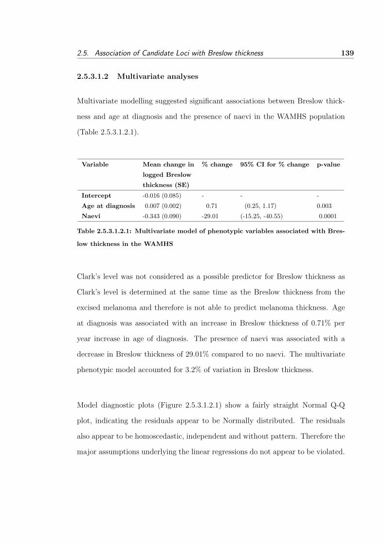
2.5. Association of Candidate Loci with Breslow thickness 139
2.5.3.1.2 Multivariate analyses
Multivariate modelling suggested significant associations between Breslow thick-
ness and age at diagnosis and the presence of naevi in the WAMHS population
(Table 2.5.3.1.2.1).
Variable Mean change in % change 95% CI for % change p-value
logged Breslow
thickness (SE)
Intercept -0.016 (0.085) - - -
Age at diagnosis 0.007 (0.002) 0.71 (0.25, 1.17) 0.003
Naevi -0.343 (0.090) -29.01 (-15.25, -40.55) 0.0001
Table 2.5.3.1.2.1: Multivariate model of phenotypic variables associated with Bres-
low thickness in the WAMHS
Clark’s level was not considered as a possible predictor for Breslow thickness as
Clark’s level is determined at the same time as the Breslow thickness from the
excised melanoma and therefore is not able to predict melanoma thickness. Age
at diagnosis was associated with an increase in Breslow thickness of 0.71% per
year increase in age of diagnosis. The presence of naevi was associated with a
decrease in Breslow thickness of 29.01% compared to no naevi. The multivariate
phenotypic model accounted for 3.2% of variation in Breslow thickness.
Model diagnostic plots (Figure 2.5.3.1.2.1) show a fairly straight Normal Q-Q
plot, indicating the residuals appear to be Normally distributed. The residuals
also appear to be homoscedastic, independent and without pattern. Therefore the
major assumptions underlying the linear regressions do not appear to be violated.
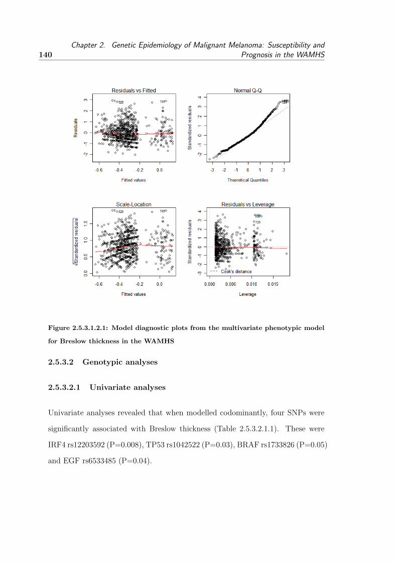
140Chapter 2. Genetic Epidemiology of Malignant Melanoma: Susceptibility and
Prognosis in the WAMHS
Figure 2.5.3.1.2.1: Model diagnostic plots from the multivariate phenotypic model
for Breslow thickness in the WAMHS
2.5.3.2 Genotypic analyses
2.5.3.2.1 Univariate analyses
Univariate analyses revealed that when modelled codominantly, four SNPs were
significantly associated with Breslow thickness (Table 2.5.3.2.1.1). These were
IRF4 rs12203592 (P=0.008), TP53 rs1042522 (P=0.03), BRAF rs1733826 (P=0.05)
and EGF rs6533485 (P=0.04).

2.5. Association of Candidate Loci with Breslow thickness 141
Gene SNP ANOVA p-value
CDC91L1 rs910873 0.32
MYH7B rs1885120 0.80
MC1R rs1805005 0.15
MC1R rs1805007 0.21
MC1R rs3212363 0.34
MC1R rs258322 0.46
MC1R rs3212369 0.48
TYR rs1042602 0.23
TYR rs1393350 0.32
TYRP1 rs1408799 0.31
KITLG rs12896399 0.64
SLC24A4 rs12821256 0.75
IRF4 rs1540771 0.11
TPCN2 rs35264875 0.14
TPCN2 rs3829241 0.94
OCA2 rs1800401 0.11
OCA2 rs1800407 0.51
OCA2 rs7495174 0.51
HERC2 rs12913832 0.37
IRF4 rs12203592 0.008
TP53 rs1042522 0.03
MTAP rs4636294 0.79
MTAP rs10757257 0.62
MTAP rs7023329 0.21
MTAP rs1011970 0.36
PLA2G6 rs2284063 0.41
PLA2G6 rs132985 0.64
BRAF rs1267635 0.69
BRAF rs1733826 0.05
BRAF rs10487888 0.57
BRAF rs17161747 0.82
BRAF rs2365151 0.87
BRAF rs17623382 0.62
BRAF rs4726020 0.37
BRAF rs6944385 0.76
EGF rs7655579 0.93
EGF rs929446 0.74
Continued on Next Page. . .

142Chapter 2. Genetic Epidemiology of Malignant Melanoma: Susceptibility and
Prognosis in the WAMHS
Table 2.5.3.2.1.1 - Continued
Gene SNP ANOVA p-value
EGF rs11568993 0.43
EGF rs882471 0.74
EGF rs4698803 0.86
EGF rs6533485 0.04
EGF rs11569121 0.80
Table 2.5.3.2.1.1: Univariate associations between Breslow thickness and SNPs modelled codom-
inantly in the WAMHS
2.5.3.2.2 Multivariate analyses
The model fitted in Section 2.5.3.1.2 formed the basis of the multivariate analysis
of the 42 genotyped genetic variants. Table 2.5.3.2.2.1 shows the coefficients for
each genotype and likelihood ratio p-values for all the SNPs, adjusted for age at
diagnosis and the presence of naevi. When modelled codominantly, three SNPs
were significantly associated with Breslow thickness at the 5% level of significance,
OCA2 rs1800401 (P=0.04), TP53 rs10425422 (P=0.009) and BRAF rs1733826
(P=0.03). Two SNPs were marginally associated with Breslow thickness, IRF4
rs12203592 (P=0.09) and EGF rs6533485 (P=0.07).
Also presented in Table 2.5.3.2.2.1 is the q-value for the FDR. After adjustment
for multiple testing, no SNPs were significantly associated with Breslow thickness.
Gene SNP Genotypes Mean change in LRT p-value q-value
logged Breslow thickness1
GG
CDC91L1 rs910873 AG 0.049 0.21 0.89
AA 0.408
GG
Continued on Next Page. . .

2.5. Association of Candidate Loci with Breslow thickness 143
Table 2.5.3.2.2.1 - Continued
Gene SNP Genotypes Mean change in LRT p-value q-value
logged Breslow thickness1
MYH7B rs1885120 CG 0.064 0.61 0.89
CC 0.138
GG
MC1R rs1805005 GT -0.004 0.18 0.89
TT 0.432
CC
MC1R rs1805007 CT -0.078 0.24 0.89
TT 0.301
AA
MC1R rs3212363 AT 0.013 0.59 0.89
TT -0.113
CC
MC1R rs258322 CT -0.020 0.62 0.89
TT 0.208
AA
MC1R rs3212369 AG -0.035 0.59 0.89
GG -0.178
CC
TYR rs1042602 AC 0.095 0.29 0.89
AA 0.081
GG
TYR rs1393350 AG -0.023 0.42 0.89
AA -0.124
CC
TYRP1 rs1408799 CT 0.031 0.52 0.89
TT -0.086
TT
SLC24A4 rs12821256 CT -0.049 0.81 0.89
CC -0.021
GG
KITLG rs12896399 GT 0.012 0.74 0.89
TT -0.046
Continued on Next Page. . .

144Chapter 2. Genetic Epidemiology of Malignant Melanoma: Susceptibility and
Prognosis in the WAMHS
Table 2.5.3.2.2.1 - Continued
Gene SNP Genotypes Mean change in LRT p-value q-value
logged Breslow thickness1
AA
IRF4 rs1540771 AG -0.124 0.16 0.89
GG -0.080
AA
TPCN2 rs35264875 AG 0.104 0.27 0.89
GG 0.024
GG
TPCN2 rs3829241 AG 0.002 1.0 1.00
AA -0.007
GG
OCA2 rs1800407 AG 0.038 0.57 0.89
AA 0.262
CC
OCA2 rs1800401 CT -0.211 0.04 0.56
TT
AA
OCA2 rs7495174 AG 0.062 0.51 0.89
GG -0.791
GG
HERC2 rs12913832 AG -0.003 0.30 0.89
AA 0.201
CC
IRF4 rs12203592 CT 0.107 0.09 0.76
TT 0.183
GG
TP53 rs1042522 CG 0.174 0.009 0.38
CC 0.208
AA
MTAP rs4636294 AG -0.050 0.65 0.89
AA 0.007
GG
MTAP rs10757257 AG -0.007 0.52 0.89
Continued on Next Page. . .

2.5. Association of Candidate Loci with Breslow thickness 145
Table 2.5.3.2.2.1 - Continued
Gene SNP Genotypes Mean change in LRT p-value q-value
logged Breslow thickness1
AA 0.088
AA
MTAP rs7023329 AG -0.060 0.32 0.89
GG 0.046
GG
MTAP rs1011970 GT -0.034 0.53 0.89
TT -0.188
AA
PLA2G6 rs2284063 AG 0.027 0.63 0.89
GG -0.066
CC
PLA2G6 rs132985 CT 0.047 0.73 0.89
TT 0.002
GG
BRAF rs1267635 AG 0.036 0.68 0.89
AA 0.186
GG
BRAF rs1733826 AG -0.150 0.03 0.56
AA -0.865
AA
BRAF rs10487888 AG -0.056 0.56 0.89
GG 0.012
GG
BRAF rs17161747 CG 0.044 0.67 0.89
CC
TT
BRAF rs2365151 CT -0.009 0.94 0.99
CC -0.267
TT
BRAF rs17623382 GT 0.005 0.50 0.89
GG -0.317
AA
Continued on Next Page. . .

146Chapter 2. Genetic Epidemiology of Malignant Melanoma: Susceptibility and
Prognosis in the WAMHS
Table 2.5.3.2.2.1 - Continued
Gene SNP Genotypes Mean change in LRT p-value q-value
logged Breslow thickness1
BRAF rs4726020 AG 0.038 0.36 0.89
GG 0.167
AA
BRAF rs6944385 AT 0.024 0.75 0.89
TT 0.179
AA
EGF rs7655579 AG 0.015 0.90 0.97
GG -0.025
CC
EGF rs929446 CT 0.040 0.68 0.89
TT -0.023
CC
EGF rs11568993 CT 0.127 0.25 0.89
TT -0.206
GG
EGF rs882471 AG 0.040 0.76 0.89
AA -0.009
TT
EGF rs4698803 AT 0.003 0.99 1.00
AA -0.013
GG
EGF rs6533485 CG 0.140 0.07 0.73
CC 0.022
GG
EGF rs11569121 AG -0.037 0.80 0.89
AA -0.184
Table 2.5.3.2.2.1: Multivariate associations between Breslow thickness and SNPs in the WAMHS
modelled codominantly
1This is the mean change in logged Breslow thickness for each genotype level, compared to
the baseline genotype.

2.5. Association of Candidate Loci with Breslow thickness 147
Analysis of the genotype coefficients determined that two of the significantly as-
sociated SNPs (rs6533485 and rs1800401) were best modelled codominantly (see
Table 2.5.3.2.2.2). The association between Breslow thickness and rs6533485 was
marginally significant (P=0.07), however only the heterozygote was significantly
associated with Breslow thickness (P=0.04).
The rs1800401 SNP did not have any rare homozygotes, however when compared
to the common homozygote, the heterozygote was significantly associated with
decreased Breslow thickness (P=0.04). This SNP accounted for 0.70% of vari-
ation in Breslow thickness. Model diagnostic plots (Figure 2.5.3.2.2.1) indicate
that the residuals appear Normally distributed, and also appear independent and
with constant variance.
SNP Genotype Mean change in % change 95% CI for % change p-value
logged Breslow
thickness1 (SE)
GG - - - -
rs6533485 CG 0.140 (0.068) 15.04 (0.72, 31.39) 0.04
CC 0.022 (0.082) 2.22 (-12.90, 19.97) 0.79
rs1800401 CC - - - -
CT -0.211 (0.100) -19.00 (-33.47, -1.37) 0.04
Table 2.5.3.2.2.2: Association between codominant SNPs and Breslow thickness in
the WAMHS, adjusted for age at diagnosis and presence of naevi
Two SNPs were best modelled additively, BRAF rs1733826 and IRF4 rs12203592,
and these results are presented in Table 2.5.3.2.2.3. Each copy of the minor allele
1This is the mean change in logged Breslow thickness for each genotype level, compared to
the baseline genotype.

148Chapter 2. Genetic Epidemiology of Malignant Melanoma: Susceptibility and
Prognosis in the WAMHS
Figure 2.5.3.2.2.1: Model diagnostic plots for the association between OCA2
rs1800401 and Breslow thickness in the WAMHS, adjusted for age at diagnosis
and presence of naevi
of the rs1733826 SNP decreased Breslow thickness, on average, by 18.06% (95%
CI = -2.70, -30.99). This SNP accounted for 0.44% of the variation in Breslow
thickness.
Conversely, each variant allele of the IRF4 rs12203592 SNP increased Breslow
thickness, on average, by 10.22% (95% CI = 1.08, 20.18). This SNP accounted
for 0.58% of variation in Breslow thickness.

2.5. Association of Candidate Loci with Breslow thickness 149
Model diagnostics for the two additive SNPs are presented in Figures 2.5.3.2.2.2
and 2.5.3.2.2.3. The residuals appear to be Normally distributed and do not ap-
pear to be violating any of the major assumptions underlying linear regression.
SNP Allele Mean change in % change 95% CI for % change p-value
logged Breslow
thickness1 (SE)
rs1733826 G - - - -
A -0.199 (0.088) -18.06 (-2.70, -30.99) 0.02
rs12203592 C - - -
T 0.097 (0.044) 10.22 (1.08, 20.18) 0.03
Table 2.5.3.2.2.3: Association between additive SNPs and Breslow thickness in the
WAMHS, adjusted for age at diagnosis and presence of naevi
One SNP was best modelled dominantly - TP53 rs1042522 - and was subject to a
significant interaction with the presence of naevi (Table 2.5.3.2.2.4). Inclusion of
the SNP and the SNP:(naevi count) interaction accounted for 1.87% of the varia-
tion in Breslow thickness. When the SNP:(naevi count) interaction was included
in the model, the presence of naevi was no longer significantly associated with
Breslow thickness (P=0.10). However, the SNP and the SNP:(naevi count) inter-
action were both significantly associated with Breslow thickness, with p-values of
0.0004 and 0.007, respectively. The interaction between TP53 rs1042522 and the
presence of naevi can be seen graphically in Figure 2.5.3.2.2.4.
Compared to a baseline model of no naevi and no variant alleles, an individual of
average age with no naevi and one of the CG or GG genotypes had, on average,
1This is the mean change in logged Breslow thickness for each variant allele.

150Chapter 2. Genetic Epidemiology of Malignant Melanoma: Susceptibility and
Prognosis in the WAMHS
Figure 2.5.3.2.2.2: Model diagnostic plots for the association between BRAF
rs1733826 and Breslow thickness in the WAMHS, adjusted for age at diagnosis
and presence of naevi
a melanoma 85% thicker. An individual with naevi and the GG genotype had
a melanoma 17% thinner, and an individual with both naevi and the GG geno-
type had a melanoma approximately 6% thicker. Therefore, there is evidence to
suggest that the effect of the TP53 rs1042522 SNP on Breslow thickness differs
according to whether an individual has naevi.
1For naevi, this is the mean change in logged Breslow thickness for individuals with naevi,
compared to individuals with no naevi. For rs1042522, this is the mean change in logged Breslow
thickness for CG+CC, compared to the baseline genotype. For rs1042522:Naevi, this is the mean
change in logged Breslow thickness for individuals with naevi and CG+CC, compared to the

2.5. Association of Candidate Loci with Breslow thickness 151
Figure 2.5.3.2.2.3: Model diagnostic plots for the association between IRF4
rs12203592 and Breslow thickness in the WAMHS, adjusted for age at diagnosis
and presence of naevi
SNP Genotype Mean change in % change 95% CI for % change p-value
logged Breslow
thickness1 (SE)
Naevi - -0.181(0.111) -16.59 (-32.93, 3.74) 0.10
rs1042522 GG - - - -
CG + CC 0.617 (0.174) 85.41 (31.88, 160.69) 0.0004
rs1042522:Naevi GG - - - -
rs1042522:Naevi CG+CC -0.495 (0.184) -39.04 (-57.54, -12.48) 0.007
Table 2.5.3.2.2.4: Association between rs1042522, modelled dominantly, and Bres-
low thickness in the WAMHS, adjusted for age at diagnosis and presence of naevi

152Chapter 2. Genetic Epidemiology of Malignant Melanoma: Susceptibility and
Prognosis in the WAMHS
Figure 2.5.3.2.2.4: Interaction between rs1042522 modelled dominantly and the
presence or absence of naevi in the WAMHS. CG+CC represents one or two copies
of the variant allele. The combination GG and no naevi forms the baseline.
Model diagnostics for the the rs1042522 model are presented in Figure 2.5.3.2.2.5.
The residuals appear to be Normally distributed and do not appear to be violating
any of the major assumptions underlying linear regression.
Modelling of Breslow thickness, with the four significant SNPS (from four genes)
and the rs1042522:(naevi count) interaction, adjusted for age at diagnosis and
the presence of naevi, found that all SNPs remained significantly associated with
Breslow thickness (P<0.05). This indicated that, before adjustment for multiple
baseline genotype and no naevi.

2.5. Association of Candidate Loci with Breslow thickness 153
Figure 2.5.3.2.2.5: Model diagnostic plots for the association between rs1052522
and Breslow thickness in the WAMHS, adjusted for age at diagnosis and presence
of naevi
testing, each SNP was an independent predictor of Breslow thickness. This final
model, including age at diagnosis, the presence of naevi and the four significant
SNPs, accounted for 6.8% of variation in Breslow thickness. However, after ad-
justment for multiple testing, these SNP associations were not significant.
154Chapter 2. Genetic Epidemiology of Malignant Melanoma: Susceptibility and
Prognosis in the WAMHS
2.5.3.3 Statistical power
2.5.3.3.1 Genetic main effects
Post-hoc statistical power analyses for an additive model with n=800 and alpha
level of 0.0012 demonstrated sufficient power (>0.80) to detect a 0.3SD change or
greater in Breslow thickness for most MAF (Figure 2.5.3.3.1.1). However, changes
in Breslow thickness of 0.1SD are not likely to have been detected by the current
study (maximum power for 0.1SD = 0.11).
Under a dominant model with n=800, there was sufficient power to detect a 0.3SD
change or greater in Breslow thickness for most MAF (Figure 2.5.3.3.1.2). How-
ever, changes in Breslow thickness of less than 0.2SD are not likely to have been
detected by the current study.
Under a recessive model with n=800, there was sufficient power to detect a 0.5SD
change in Breslow thickness for MAF > 0.30. (Figure 2.5.3.3.1.3). However,
changes in Breslow thickness of less than 0.5SD would likely not be detected.
2.5.3.3.2 Gene-environment interactions
Post–hoc statistical power analyses for an additive model with n=800, alpha level
of 0.0006, and environment exposure prevalence of 0.2 demonstrated sufficient
power (>0.80) to detect a 0.5SD change or greater in Breslow thickness for MAF
0.3 and greater (Figure 2.5.3.3.2.1). However, other combinations of MAF and
changes in Breslow thickness are not likely to have been detected by the current
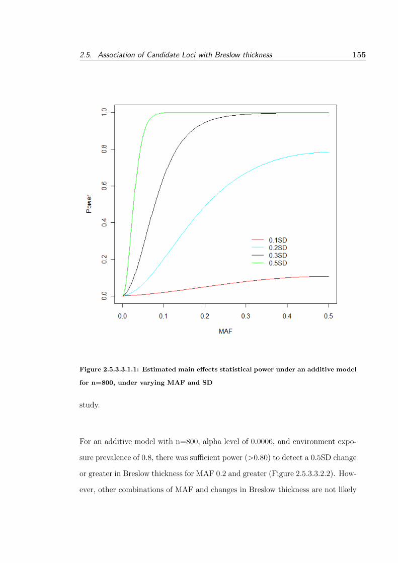
2.5. Association of Candidate Loci with Breslow thickness 155
Figure 2.5.3.3.1.1: Estimated main effects statistical power under an additive model
for n=800, under varying MAF and SD
study.
For an additive model with n=800, alpha level of 0.0006, and environment expo-
sure prevalence of 0.8, there was sufficient power (>0.80) to detect a 0.5SD change
or greater in Breslow thickness for MAF 0.2 and greater (Figure 2.5.3.3.2.2). How-
ever, other combinations of MAF and changes in Breslow thickness are not likely

156Chapter 2. Genetic Epidemiology of Malignant Melanoma: Susceptibility and
Prognosis in the WAMHS
Figure 2.5.3.3.1.2: Estimated main effects statistical power under a dominant model
for n=800, under varying MAF and SD
to have been detected by the current study.
2.5.3.4 Summary of results
Four SNPs (from four different genes - IRF4, TP53, OCA2 and BRAF) were as-
sociated with Breslow thickness when modelled multivariately (Table 2.5.3.4.1).
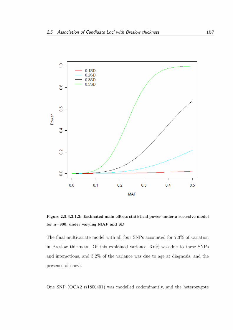
2.5. Association of Candidate Loci with Breslow thickness 157
Figure 2.5.3.3.1.3: Estimated main effects statistical power under a recessive model
for n=800, under varying MAF and SD
The final multivariate model with all four SNPs accounted for 7.3% of variation
in Breslow thickness. Of this explained variance, 3.6% was due to these SNPs
and interactions, and 3.2% of the variance was due to age at diagnosis, and the
presence of naevi.
One SNP (OCA2 rs1800401) was modelled codominantly, and the heterozygote

158Chapter 2. Genetic Epidemiology of Malignant Melanoma: Susceptibility and
Prognosis in the WAMHS
Figure 2.5.3.3.2.1: Estimated interaction effects statistical power under an addi-
tive model for n=800, under varying MAF and SD for environmental exposure
prevalence of 0.2
genotype was associated with a decrease in Breslow thickness. Two SNPs were
modelled additively, with the variant allele associated with a thinner melanoma for
BRAF rs1733826, and a thicker melanoma for IRF4 rs12203592. The remaining
SNP, TP53 rs1042522, was modelled dominantly, with the variant allele associ-
ated with a thicker melanoma, which was moderated by the presence of naevi.

2.5. Association of Candidate Loci with Breslow thickness 159
Figure 2.5.3.3.2.2: Estimated interaction effects statistical power under an addi-
tive model for n=800, under varying MAF and SD for environmental exposure
prevalence of 0.8
However, after adjusting for multiple testing using the FDR, none of these asso-
ciations were significant at the 5% significance level.
The rs6533485 SNP was significant (without adjustment for multiple testing) when
modelled univariately, however it was not significant when adjusted for age at di-

160Chapter 2. Genetic Epidemiology of Malignant Melanoma: Susceptibility and
Prognosis in the WAMHS
agnosis and naevi, and is therefore not discussed further.
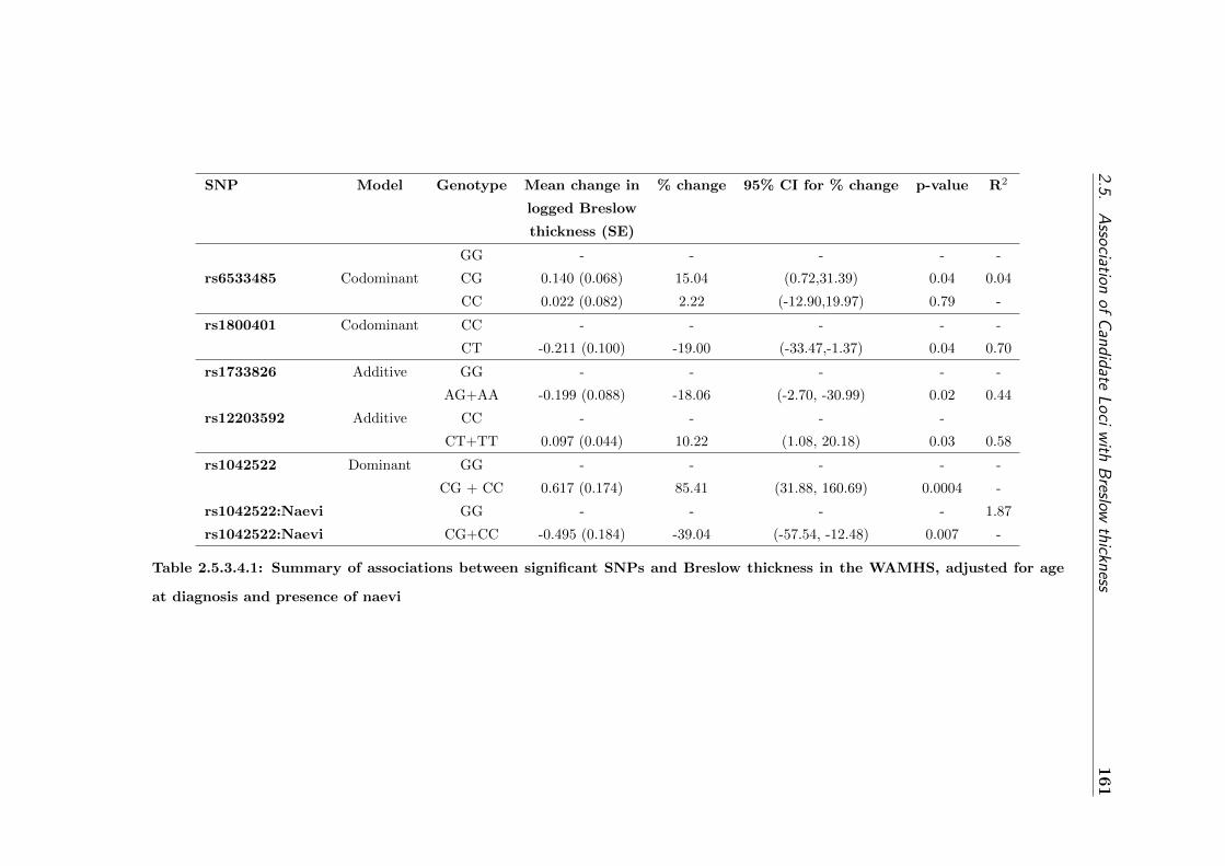
2.5.A
ssociation
ofC
andidateL
oci
with
Breslow
thickness161
SNP Model Genotype Mean change in % change 95% CI for % change p-value R2
logged Breslow
thickness (SE)
GG - - - - -
rs6533485 Codominant CG 0.140 (0.068) 15.04 (0.72,31.39) 0.04 0.04
CC 0.022 (0.082) 2.22 (-12.90,19.97) 0.79 -
rs1800401 Codominant CC - - - - -
CT -0.211 (0.100) -19.00 (-33.47,-1.37) 0.04 0.70
rs1733826 Additive GG - - - - -
AG+AA -0.199 (0.088) -18.06 (-2.70, -30.99) 0.02 0.44
rs12203592 Additive CC - - - -
CT+TT 0.097 (0.044) 10.22 (1.08, 20.18) 0.03 0.58
rs1042522 Dominant GG - - - - -
CG + CC 0.617 (0.174) 85.41 (31.88, 160.69) 0.0004 -
rs1042522:Naevi GG - - - - 1.87
rs1042522:Naevi CG+CC -0.495 (0.184) -39.04 (-57.54, -12.48) 0.007 -
Table 2.5.3.4.1: Summary of associations between significant SNPs and Breslow thickness in the WAMHS, adjusted for age
at diagnosis and presence of naevi

162Chapter 2. Genetic Epidemiology of Malignant Melanoma: Susceptibility and
Prognosis in the WAMHS
2.5.4 Discussion
2.5.4.1 Introduction
The aim of the analyses presented in this section was to investigate associations
between 42 identified melanoma-risk candidate SNPs and melanoma prognosis
in the WAMHS sample. In this study, four loci were significantly associated
with melanoma prognosis, however these associations become non-significant after
adjustment for multiple testing. These associations and their implications are
discussed further in Section 2.5.4.3 (please see page 171).
2.5.4.2 Summary of population characteristics
The WAMHS sub-sample used in this analysis were 800 Caucasian individuals who
were diagnosed with an invasive melanoma between January 2006 and September
2009. To be eligible for inclusion in this analysis, subjects were required to have a
Breslow thickness recorded, as this was the outcome variable. Breslow thickness
and associations between phenotypic variables and Breslow thickness are discussed
in this section.
2.5.4.2.1 Breslow thickness
Breslow thickness was the outcome variable in these analyses and was used as a
surrogate for melanoma prognosis. There is continued debate over whether Bres-
low thickness is a measure of the time from melanoma development to examination
and diagnosis by a physician (‘diagnosis delay’), a measure of the biological ag-
gressivity of the tumour, or a combination of both [182–188].

2.5. Association of Candidate Loci with Breslow thickness 163
The relationship between Breslow thickness, diagnosis delay and aggressiveness
of the tumour is complex. It is difficult to accumulate sufficient evidence to re-
ject the hypotheses that Breslow thickness is not a proxy for either the biological
aggressiveness of the melanoma tumour, or diagnosis delay, as prospective stud-
ies to evaluate the natural history of a melanoma tumour from its onset raises
both practical and ethical issues. Studies investigating these relationships must
rely on patients to recall when they first noticed the new lesion or the change in
a pre-existing lesion. These studies also assume that when the melanoma first
developed, there was some noticeable change to the skin that was recognised by
the patient. However, for melanomas arising on areas of the body that are not
frequently viewed, such as the back, the tumour may remain undetected for some
time.
Within these framework limitations, several studies have attempted to investigate
the relationship between tumour thickness, delay in diagnosis and the aggres-
siveness of the tumour. However, these studies have failed to identify a clear
association between thicker melanomas and a longer delay of diagnosis [182–188].
The largest of these studies, by Richard et al. [187], investigated the correlation
between Breslow thickness and diagnosis delay in a sample of 590 French indi-
viduals (57.6% female, mean age of 51.2 years, and median Breslow thickness of
1.13 mm). Richard et al. found some evidence for a positive correlation (r=0.17,
P=0.009) between Breslow thickness and the time the subject noticed the lesion
to the time the subject became suspicious of the lesion. However, this association
depended greatly on the thickness of the melanoma. For tumours less than 3mm
thick, thicker melanoma tumours were associated with an increase in diagnosis
164Chapter 2. Genetic Epidemiology of Malignant Melanoma: Susceptibility and
Prognosis in the WAMHS
delay, while for tumours greater than 3mm thick, thicker melanoma tumours were
associated with a decrease in diagnosis delay. Additionally, a negative correlation
was observed between the time the subject became suspicious of the lesion and
the first examination of the lesion by a physician, and Breslow thickness (r=-0.20,
p<0.001). These results suggest that Breslow thickness may be a result of both
diagnosis delay, and also the aggressiveness of the tumour.
Furthermore, Richard et al. suggested that in populations uninformed about
melanoma and the importance of skin examinations, diagnosis delay is possibly
the main factor responsible for tumour thickness, while in informed populations,
the biological behaviour of the tumour may be the major factor affecting tumour
thickness. Australia has had a large number of public education campaigns, par-
ticularly over the past 25 years [189]. These numerous campaigns, primarily run
by the Cancer Council of Australia, would suggest that Australia is an informed
population. As such, in Australian communities of informed individuals, Breslow
thickness is more likely to be a measure of the agressiveness of the melanoma
tumour.
The most recent study by Lui et al [188] investigated tumour rate of growth (es-
timated by Breslow thickness divided by delay in diagnosis) in a sample of 404
Australian individuals (45.0% female, mean age of 54.2 years, and median Bres-
low thickness of 1.14 mm). Liu et al. found that the rate of growth was highly
associated with thicker melanomas, providing evidence to suggest that thicker
melanomas are thicker as they have grown faster, not because there has been a
delay in diagnosis.

2.5. Association of Candidate Loci with Breslow thickness 165
If Breslow thickness is solely a measure of diagnosis delay, then the observed as-
sociations in this study between Breslow thickness, age at diagnosis, naevi and
several SNPs would represent associations between these variables and diagnosis
delay. However, if Breslow thickness is a measure of the aggressiveness of the
tumour, then these observed associations would represent associations between
these variables and melanoma prognosis. If the latter is true, then this study will
allow the identification of individuals who are at higher risk of melanoma with a
poorer prognosis.
Without the use of prospective, longitudinal cohort studies, it is difficult to assess
the relationship between Breslow thickness and the aggressiveness of the tumour
with any certainty. However, there is some evidence to suggest that Breslow thick-
ness is a sensible measure for melanoma growth and prognosis, and is largely de-
pendent on the aggressiveness of the tumour. Therefore, the identification of phe-
notypic variables and genetic variants that are associated with Breslow thickness
is important as it may help to identify individuals at risk of poor melanoma prog-
nosis, and may also elucidate the biological mechanisms underpinning melanoma
growth.
In the current study, Breslow thickness was analysed as a continuous variable. In
previous studies, convention has been to categorise Breslow thickness using cut-
points which represent staging classifications [153]. A review of melanoma studies
by Vollmer et al. [190] found that in these studies, Breslow thickness was cate-
gorised with as few as one cutpoint, and as many as seven. However, it is unclear
if natural cutpoints exist and if so, which cutpoints are optimal for modelling
Breslow thickness. Analyses by Vollmer et al. and Stadelmann et al. [191] found

166Chapter 2. Genetic Epidemiology of Malignant Melanoma: Susceptibility and
Prognosis in the WAMHS
that using Breslow thickness as a continuous variable more clearly modelled sur-
vival, than using various different cutpoints to create arbitrary categories.
In addition, the use of continuous outcomes in genetic association studies is of-
ten more powerful and informative than categorising outcomes [192]. However,
Breslow thickness is still often categorised [112, 129, 158, 193, 194]. This may be
due to various reasons, such as the ability to easily match thickness categories to
treatment. It may also be categorised due to the high positive skewness of Breslow
thickness measurements, with a large number of thin melanomas (< 1mm). In this
thesis, the natural log transformation sufficiently transformed Breslow thickness,
and modelling Breslow thickness this way did not appear to violate any linear
regression assumptions.
Median Breslow thickness in this study was 0.65. The comparison of this median
thickness with median thicknesses from other studies is difficult due to the conven-
tion of reporting Breslow thickness as a categorical variable. In addition, median
Breslow thickness has decreased over the past few decades due to the increase
in diagnosis of thin melanomas [195], which further compounds the difficultly in
comparing Breslow thickness in this study with earlier studies. However, the few
recent studies which have published median Breslow thickness found similar me-
dians of 0.55 mm [112], 0.6 mm [196] and 0.56 mm [112]. Therefore, the median
Breslow thickness in this study appears comparable to other studies.
Furthermore, analysis of Breslow thickness between the eligible population and
the WAMHS sub-sample from Section 2.3.4 found that median Breslow thickness

2.5. Association of Candidate Loci with Breslow thickness 167
in the sample did not differ significantly from the median Breslow thickness of all
adult individuals diagnosed with melanoma in Western Australia from January
2006 and September 2009.
Therefore, the distribution of Breslow thickness in this study appears compa-
rable to Breslow thickness described in Australian and international studies of
melanoma cases. This indicates that the associations observed in this study be-
tween Breslow thickness and age at diagnosis, the presence of naevi and several
genetic variants may be generalisable back to melanoma cases in Caucasian indi-
viduals world-wide.
2.5.4.2.2 Sex
No association was observed between Breslow thickness and sex in this study.
Median Breslow thickness for males was 0.63, compared to a median thickness
for females of 0.65, however this association was not statistically significant. This
thicker Breslow thickness for females contradicts other studies which have found
males tend to have thicker melanomas [150, 152, 154, 155]. Further analysis (not
shown) found that for the eligible population, the median Breslow thickness was
0.67 mm (range of 0.04 mm to 35.00 mm) for males and 0.60 mm (range of 0.10
mm to 23.00 mm) for females. Therefore, it appears that the sub-sample used
in this analysis was not representative of the eligible population, and included
a greater proportion of women with thicker melanomas, when compared to the
eligible population. However, it is unlikely that this had a great effect on the
analysis as sex was not significantly associated with Breslow thickness, and no
sex interactions with either age at diagnosis, the presence of naevi, or any genetic
variants were identified.
168Chapter 2. Genetic Epidemiology of Malignant Melanoma: Susceptibility and
Prognosis in the WAMHS
2.5.4.2.3 Age at diagnosis
Age at diagnosis was significantly associated with Breslow thickness. In this study,
each year of age resulted in an average increase in Breslow thickness of 0.71%,
when adjusted for the presence of naevi. Breslow thickness has been associated
with age at diagnosis in previous studies [149–153], in particular, with older indi-
viduals being diagnosed with thicker melanomas. One reason for this, suggested
by Hanrahan et al. [197], is that older individuals are less likely to notice changes
in melanoma, and are therefore less likely to have their tumours detected and
subsequently diagnosed.
However, as previously described, evidence suggests that melanoma thickness is
not solely related to diagnosis delay, and therefore this argument does not appear
to be wholly valid. In their study of rate of growth of melanoma, Liu et al. [188]
found that individuals aged over 70 years had higher rates of melanoma growth,
when compared to individuals aged under 70 years. As rate of growth is believed
to be an independent risk factor for Breslow thickness, it is therefore possible that
older individuals would have thicker melanomas. However, the evidence is not
clear and older individuals being diagnosed with thicker melanomas may be due
to a combination of these higher rates of tumour growth and a reduced ability for
older individuals to detect changes in melanoma.
2.5.4.2.4 Naevi
The presence of multiple naevi is the principle risk-factor for melanoma. In this
study, 75% of subjects considered their bodies to have ‘Few’ or ‘Some’ naevi, 14%
had ‘Many’ naevi and only 11% had ‘None’. The median number of naevi on the
2.5. Association of Candidate Loci with Breslow thickness 169
upper back was four, while the median number of naevi on the lower back was five.
The number of naevi on either section of the back was not significantly associated
with Breslow thickness. The four categories of naevi counts, ranging from ‘Few’
to ‘Many’ were also not significantly associated with Breslow thickness. This vari-
able was then transformed into a binary trait - the presence of naevi - which was
recorded as ‘No’ or ‘Yes’, and this new variable was significantly associated with
Breslow thickness.
In this study, having no naevi resulted in an increase of Breslow thickness of 29%,
when compared to having naevi, adjusted for age at diagnosis. While this supports
the hypothesis that melanoma risk factors will also be associated with melanoma
prognosis, the direction of the association is contrary to what may be expected.
That is, it seems more plausible that thicker melanomas would be associated with
more naevi, not that thicker melanomas are associated with fewer naevi.
In their study of Breslow thickness, Liu et al. [188] found a significant association
between the rate of growth of melanoma, and naevi. In particular, individuals
with fewer naevi had a faster melanoma growth rate and individuals with more
naevi had a slower melanoma growth rate.
One reason for the inverse relationship between naevi count and melanoma growth
rate may be that thicker melanomas tend to be the nodular type [198] and these
are associated with fewer naevi. In this study, the types of melanoma were not
available directly from the WACR as they are not uniformly recorded on pathology
forms, however it may be possible to obtain this information. If it was possible

170Chapter 2. Genetic Epidemiology of Malignant Melanoma: Susceptibility and
Prognosis in the WAMHS
to adjust for the type of melanoma, then the association between fewer naevi and
thicker melanomas may no longer be observed.
Another reason for this inverse relationship may be that individuals with many
naevi may be more likely to visit their doctor and be screened for melanoma. This
may result in individuals with naevi having thinner melanomas diagnosed, which
would result in naevi appearing to be associated with thinner melanomas.
The number of naevi on the back was not associated with melanoma thickness,
while the presence of naevi was associated with melanoma thickness. This discrep-
ancy may be explained by the way naevi were reported. In this study, subjects or
a family member of the subject were asked to count the number of naevi on two
sections of the back. The subject was sent an information sheet explaining how
to identify naevi, however anecdotal evidence suggested that WAMHS subjects
found it difficult to identify naevi. This may be as the back is a difficult area to
examine, and there may also be a large amount of freckling which may be confused
with naevi. Therefore, the naevi counts on the back may not be wholly reliable.
However, when the subject examined four different diagrams representing degrees
of naevi on the whole body, ranging from ‘None’ to ‘Many’, their responses may
have been more accurate and less likely to be subjected to biases. In particular,
it may have been easier for an individual to identify themselves as having ‘No’
naevi, while the categories ‘Few’, ‘Some’ or ‘Many’, may have been more difficult
to choose between.

2.5. Association of Candidate Loci with Breslow thickness 171
The only way to determine if the naevi counts were accurate would be for a
trained individual to count the number of naevi on subjects’ backs for a subset
of the sample. The concordance between the counts performed by an expert and
those performed by the subject could be measured to identify how accurately naevi
were counted. As part of the scar examination which some subjects underwent
as part of the WAMHS, each subject’s back was photographed. Therefore, it is
possible to estimate the concordance between self-reported naevi counts and those
identified by a trained individual. This was beyond the scope of the present study,
however it would make for interesting further research.
2.5.4.3 Summary of genetic association analyses
2.5.4.3.1 Review of genetic variants studied
Forty two genetic polymorphisms in 16 candidate genes and their associations with
Breslow thickness were analysed in the current study. Twenty three of these SNPs
were chosen as they had been identified as melanoma-risk SNPs in earlier GWAS
and candidate-gene studies, or were associated with melanoma-risk factors, such
as light pigmentation and naevi. The remaining nineteen SNPs were tag-SNPs
derived from HapMap [175] in the EGF, BRAF and MC1R genes.
2.5.4.3.2 Details of associations
After adjustment for age at diagnosis and naevi, four SNPs provided some evidence
for association with Breslow thickness. These SNPs were rs1800401 in the OCA2
gene, rs1042522 in the TP53 gene, rs12203592 in the IRF4 gene and rs1733826 in
the BRAF gene. After adjustment for multiple testing, none of these associations
remained significant. Therefore, it is possible that the associations detected were
172Chapter 2. Genetic Epidemiology of Malignant Melanoma: Susceptibility and
Prognosis in the WAMHS
false positives. However under different conditions, such as a larger sample size,
these associations may have remained significant after multiple testing.
Prior to this study, associations between these SNPs and Breslow thickness had
not been investigated. Therefore, the results of the current association study are
novel and warrant further investigations, including replication of these associations
in a larger sample.
2.5.4.3.2.1 OCA2
The rs1800401 SNP was modelled codominantly, with the heterozygote associ-
ated with a 19% thinner melanoma, compared to the major homozygote. The
rs1800401 SNP is located in the OCA2 (oculocutaneous albinism) gene on chro-
mosome 15q11. Mutations in OCA2 have been associated with albinism [199,200]
and pigmentation [169,201,202]. In particular, the ‘A’ allele of the rs1800401 SNP
was associated with greater odds of having brown or black eyes [169], or reduced
odds of having lighter eye colours. Lighter eyes are thought to be a melanoma-risk
factor, in particular, blue eyes have been identified as a melanoma risk factor [89],
therefore the ‘A’ allele would likely be associated with reduced melanoma risk. In
this thesis, the complementary DNA strand was analysed (‘T’ allele), and this ‘T’
allele was associated with thinner melanoma. Therefore the risk allele (‘T’ or ‘A’)
is associated with lower melanoma risk, and also thinner melanomas.
It is interesting to note that no subjects in this thesis were rare homozygotes for
this SNP. This was also observed in a study by Duffy et al. [203] of Australian
twin families without melanoma, where 1,268 were common homozygous, 136 were
2.5. Association of Candidate Loci with Breslow thickness 173
heterozygous, and none were rare homozygous.
2.5.4.3.2.2 TP53
The rs1042522 SNP in the TP53 gene was modelled dominantly, with one or two
copies of the variant C allele associated with thicker melanoma. This relationship
was moderated by the presence of naevi, with the ‘C’ variant associated with 85%
thicker melanomas if no naevi, and 6% thicker melanomas with some naevi, when
compared to having no variant alleles and no naevi.
The TP53 gene is found on chromosome 17p31.1, and encodes the tumour sup-
pressor protein p53. P53 plays a critical role in preventing cancer development, in
particular by preventing tumour cell growth [204]. Mutations in TP53 have been
associated with a wide spectrum of cancers, including Li-Fraumeni syndrome [205],
breast cancer, and leukemia, and is also associated with early onset cancer [206].
The most common polymorphism is rs1042522, and this has been found to be
associated with melanoma prognosis in several studies [172, 207–209]. However,
these associations have been contradictory, with two studies identifying the ‘C’ al-
lele as the risk allele [207,208], and the other two studies identifying the ‘A’ allele
as the risk allele [172, 209]. Further replication is therefore required to reconcile
these findings.
Few investigations have studied the relationship between naevi and TP53, however
there is some evidence of somatic mutations of TP53 in naevi [210]. In addition,
a linkage study of naevi by Zhu et al. [211] identified a region of chromosome 17

174Chapter 2. Genetic Epidemiology of Malignant Melanoma: Susceptibility and
Prognosis in the WAMHS
which was linked with naevi, which may have been due to TP53.
The association between Breslow thickness and the rs1042522 SNP is unclear, and
further research is required to unravel the relationship between Breslow thickness,
naevi and TP53.
2.5.4.3.2.3 IRF4
The rs12203592 SNP in the IRF4 gene was modelled additively, with each ‘T’
variant allele associated with a 10% thicker melanoma. The ‘T’ variant of the
rs12203592 SNP has been associated with many pigmentation factors, such as
blonde hair, light skin colour, light eye colour and an inability to tan [124], which
are known melanoma-risk factors. Therefore, it appears that the ‘T’ variant is
associated with both melanoma risk and also thicker melanomas.
The IRF4 (Interferon Regulatory Factor 4) gene is located on chromosome 6p25.3,
and encodes the IRF4 protein. This protein regulates the transcription of inter-
feron proteins which are made and released in response to pathogens, including
tumour cells [124].
The IRF4 gene was first shown to be associated with pigmentation factors in a
2007 GWAS by Sulem et al. [109]. Subsequent to this GWAS, a second GWAS
of pigmentation in 2008 [124] found the rs12203592 SNP on the IRF4 gene to be
associated with pigmentation factors and skin tanning response to sunlight. In
their paper, Han et al. [124] reported that this association had been replicated
in several studies. IRF4 encodes the B-cell protein which has been proposed as

2.5. Association of Candidate Loci with Breslow thickness 175
a marker for both primary and metastatic melanoma and benign naevi [212].
However, the role of IRF4 in pigmentation and therefore melanoma risk, is still
generally not understood.
2.5.4.3.2.4 BRAF
The rs1733826 SNP in the BRAF gene was associated with a decrease in Breslow
thickness, in particular, each copy of the ‘A’ allele decreased Breslow thickness by
18%.
The BRAF gene is located on chromosome 7q34 and encodes the B-RAF protein.
This protein is associated with serine/threonine kinase activities, and mediates
signals involving cell growth, transformation and differentiation [272]. Somatic
mutations in BRAF have been identified in many cancers, including melanoma,
lung cancer, and colorectal cancer [213]. Associations between germline mutations
in BRAF have been detected [130,214], however other studies have not found any
association [215,216], and therefore the role of BRAF as a melanoma-susceptibility
gene is still largely unclear.
No associations have been detected between somatic mutations in BRAF and
Breslow thickness [217]. However, to the author’s knowledge, no associations
between germline mutations and Breslow thickness have been investigated before
this study.
176Chapter 2. Genetic Epidemiology of Malignant Melanoma: Susceptibility and
Prognosis in the WAMHS
2.5.4.4 Causality
The set of criteria described by Hill and explained earlier in Section 1.1.1 can
be used to investigate if the associations observed in this thesis may be causal.
These criteria include strength, consistency and temporality. The strength of the
associations between genetic variants and Breslow thickness were not strong, with
each variant only associated with a small change in Breslow thickness.
Consistency of these associations is difficult to determine as the genetic vari-
ants identified in this study as associated with Breslow thickness have not been
replicated in other studies to date. Temporality is easier to identify in genetic
association studies, as genotypes are assigned to offspring from parental germline
DNA at conception, and therefore the genotype must predate the development of
melanoma.
The observed associations do not appear to violate Hill’s criteria. However, due
to the millions of common SNPs in the human genome, it is unlikely that any of
the variants found to be associated with Breslow thickness are themselves causal
variants. If the observed associations are true, it is more likely that these variants
are simply markers in LD with nearby causal variants.
2.5.4.5 Potential limitations
As with all genetic association studies, this study has potential limitations, in-
cluding the use of self-reported variables, low statistical power, and the possibility
of population stratification.

2.5. Association of Candidate Loci with Breslow thickness 177
All variables collected as part of the WAMHS questionnaire were self-reported.
This included relatively easy to measure data, such as height and weight, and also
more difficult to recall measures such as sun exposure. The use of self-reported
data has been extensively studied [169,218–222]. Sun exposure is notoriously dif-
ficult to measure, and there is debate surrounding the reliability and validity of
sun exposure recollection [70,219,221]. It is possible that sun exposure, sometimes
from decades earlier, cannot be reliably recalled. In this study, we attempted to
minimise recall bias due to sun exposure measures by using events such as blis-
tering sunburn, which may be recalled more easily than total time spent in the
sun. One way to reduce recall bias would be to conduct a prospective study of a
sample from the general population, where a group of individuals is followed, and
their sun exposures are measured. This would negate the need for individuals to
recall their sun exposure from years earlier. However, as melanoma is a relatively
rare disease, thousands of individuals would need to be followed-up in order to
obtain an adequate sample size of melanoma cases.
Many other variables were also self-reported, including height, weight, naevi
counts and pigmentation traits. It is possible that all of these were not mea-
sured reliably. Measurement error could be reduced if trained individuals were
employed by the study to measure these traits, however this would likely be more
costly, and time-consuming for the study.
The measure of freckling used in this thesis was taken from an estimate of freckling
on the face. Freckling on the face has been shown to be highly correlated with
freckling on other anatomic sites, including the arms and back [280]. Therefore,
freckling on the face, which is easy to measure, was used as a proxy for freckling

178Chapter 2. Genetic Epidemiology of Malignant Melanoma: Susceptibility and
Prognosis in the WAMHS
on other anatomic sites.
Ethnicity collected as part of the WAMHS was also self-reported. Subjects were
asked their ethnicity and their parents’ ethnicity. If either of these was non-
Caucasian, the subject was not considered Caucasian and was not included in
the analyses for this thesis. In a study of self-reported ethnicity, Mez et al. [223]
found self-reported ethnicity was a reasonable proxy for genetic ancestry [223].
In addition, any bias due to population stratification is likely to be small [224],
particularly for well conducted and analysed studies. However, there is a possibil-
ity that self-reported ethnicity, along with other self-reported variables were not
reliably measured.
The inclusion of only Caucasian individuals in the study also means that the
genetic association results are only relevant to Caucasian populations. Further
replication in other ethnic groups is required in order to generalise these results
back to different ethnic groups.
Another limitation of this study is the relatively small sample size, resulting in
modest statistical power. At this start of this thesis, it was estimated that with
1,000 melanoma cases diagnosed in Western Australia each year, approximately
2,000 individuals would be recruited and available for use in this thesis. However,
due to a number of issues with data collection, recruitment took longer than
expected and therefore only 800 individuals were able to be included in this thesis
which will have reduced statistical power substantially. Power analyses showed
that for an additive genetic model, for SNPs with a MAF greater than 0.2, this

2.5. Association of Candidate Loci with Breslow thickness 179
sample would only be sufficiently powered to detect a change in Breslow thickness
of more than 0.2SD (1.3% of variance). Therefore, the study was unable to detect
small genetic effects. Replication is therefore required in larger sample sizes which
would be more adequately powered.
2.5.5 Summary
In this section, possible associations between Breslow thickness and phenotypic
variables and genotypic variants were investigated. Two phenotypic variables
were significantly associated with Breslow thickness. These were age at diagnosis,
where older age of diagnosis was associated with thicker melanomas, and the pres-
ence of naevi, which was associated with thinner melanomas. The use of Breslow
thickness as a proxy for progression of the tumour means that these factors would
likely also be associated with melanomas which tend to grow faster.
In addition, four SNPs were found to be associated with Breslow thickness. Fur-
ther replication of these results is necessary, as after adjustment for multiple test-
ing, none of these associations remained significant. However, this study has
provided some evidence for the role of four genes in melanoma prognosis, which
may lead to an increased understanding of the mechanisms by which melanomas
grow. The results of this study will also assist with identifying individuals who
are at a higher risk of thicker melanomas, and therefore, poorer prognosis.
In total, age at diagnosis, the presence of naevi, and the four SNPs accounted
for 6.8% of variation in Breslow thickness. This means there is a large amount
of variation which is as yet unaccounted for. This is likely to include many other
180Chapter 2. Genetic Epidemiology of Malignant Melanoma: Susceptibility and
Prognosis in the WAMHS
SNPs, and also environment and host factors. Further studies of other genes,
and collection of more phenotypic data in larger samples may assist in elucidating
the role of these phenotypic and genetic variables in melanoma development and
prognosis.
2.6 Chapter Summary
Melanoma is a significant public health issue in Australia, particularly in Western
Australia. In Western Australia, more than 1,000 individuals are diagnosed with
melanoma each year, accounting for approximately 10% of all cancer diagnoses.
Invasive melanoma is an aggressive form of skin cancer, and it is expected that
Australian incidence and mortality rates from this disease will continue to rise [51].
The main environmental risk factor for melanoma is sun exposure, and the main
host risk factor is the presence of naevi, however the association of other risk-
factors with melanoma risk is uncertain and many associations have not been
consistently replicated. Several genetic variants which contribute to melanoma
risk have been identified, however, these account for only a small proportion of
melanoma diagnoses. In addition, the role of specific genetic and environmental
factors in melanoma prognosis are largely unknown. Therefore, the collection of
genetic epidemiological data from melanoma cases is required, along with further
investigations in order to elucidate the role of environmental, host and genetic
risk factors in melanoma-susceptibility and prognosis.
This chapter described the establishment of the WAMHS, and the use of these
data to conduct genetic epidemiological associations into melanoma susceptibility

2.6. Chapter Summary 181
and prognosis.
The WAMHS is a population-based case-collection and biospecimen resource com-
prised of consenting adults diagnosed with melanoma in Western Australia be-
tween January 2006 and September 2009. WAMHS subjects completed a ques-
tionnaire and also gave a blood sample for DNA, serum, and an additional blood
sample for RNA. The final sample consisted of 1,643 participants, with 1,157 hav-
ing complete questionnaire data and blood samples. This is the largest population-
based study of melanoma cases in Western Australia, and one of the largest in
the world. As such, the WAMHS is an ideal resource for genetic epidemiological
investigations into melanoma susceptibility and prognosis.
As part of this PhD, 42 SNPs in 16 genes were genotyped in the WAMHS sample.
The SNPs were chosen on the basis that they were in or close to loci which have
been previously identified as melanoma-risk genes. The association of these SNPs
and melanoma-susceptibility were investigated by comparing the genotypic dis-
tributions of the WAMHS cases, with the genotypic distributions of two general
population samples - the HapMap-CEU and the BHS samples. After adjustment
for multiple testing, the association of six SNPs in five genes with melanoma
risk was replicated, with only two SNPs associated when compared to both the
HapMap-CEU and BHS control populations.
In this chapter, possible associations between these 42 melanoma-risk SNPs and
Breslow thickness were also investigated. Melanoma prognosis was determined by
Breslow thickness, with a thicker Breslow thickness indicating a poorer progno-

182Chapter 2. Genetic Epidemiology of Malignant Melanoma: Susceptibility and
Prognosis in the WAMHS
sis. Phenotypic analyses found increasing age at diagnosis was associated with
thicker Breslow thickness, and therefore poorer prognosis, while the presence of
naevi was associated with thinner melanomas, and therefore a better prognosis.
Four SNPs were associated with Breslow thickness, however after adjustment for
multiple testing, none of these associations remained significant.
One SNP - rs12203592 in the IRF4 gene - was associated with melanoma risk
in the WAMHS sample, compared to both the HapMap and BHS control sam-
ples, and was also associated with thicker melanomas in the WAMHS sample. In
particular, the ‘T’ allele was associated with both increased melanoma risk, and
thicker melanomas. However, the latter association was not significant after ad-
justment for multiple testing. No other SNPs were consistent in their associations.
It is possible that genetic variants which increase melanoma-susceptibility are
also associated with thicker Breslow thickness and therefore poorer prognosis.
However, the current study had several limitations, and was not able to provide
sufficient evidence to support this hypothesis. Replication of these genetic results,
particularly in larger samples, is required.

183CHAPTER 3
Mendelian Randomisation: An Application of
Instrumental Variable Techniques
3.1 Introduction
‘Mendelian randomisation’ is an application of a technique known as instrumental
variables (IVs), which can be used to better understand and model causality in
epidemiological studies. In this chapter I provide a background for IV methods
and Mendelian randomisation, including their advantages and disadvantages. I
also describe a novel implementation of Mendelian randomisation analyses incor-
porating haplotypes in a software library for R, MRsnphap.
When this thesis was being planned, I intended to investigate causal pathways
underlying melanoma. Mendelian randomisation approaches were therefore at-
tractive as they would have allowed me to investigate such pathways assuming the
conditions for Mendelian randomisation analyses were met (these are described
further in Section 3.4.2). One potential analysis was to investigate the effect of
serum vitamin D levels on Breslow thickness in the WAMHS cases, and if an as-
sociation was detected, to investigate whether this association was causal. The
rationale for this is discussed further in Section 3.2. Due to financial constraints,
vitamin D levels in the WAMHS were not measured, and therefore this analysis
was not able to be performed. However, this example is used throughout this
section to illustrate the possible use of Mendelian randomisation studies using
melanoma cases from the WAMHS.

184Chapter 3. Mendelian Randomisation: An Application of Instrumental Variable
Techniques
3.2 Vitamin D Levels and Breslow Thickness
Vitamin D is a fat-soluble secosteroid and is a term generally used to refer to
vitamin D2 and/or vitamin D3. Vitamin D3 is produced when the skin is ex-
posed to sunlight, in particular, ultraviolet-B radiation. In recent years, vitamin
D levels, in particular vitamin D deficiency has been linked to increased risks of
chronic disease, including osteoarthritis, diabetes, prostate cancer, breast cancer,
and melanoma [277].
Vitamin D levels have been associated with both melanoma susceptibility and
prognosis [263]. In particular, increased vitamin D levels are associated with a
lower risk of melanoma recurrence, and thinner melanomas. Vitamin D levels are
often higher in individuals with substantial sun exposure, as exposure to ultra-
violet radiation leads to an increased production of vitamin D. Therefore, this
association suggests that individuals with higher vitamin D levels (and higher
ultraviolet radiation exposure) are at a lower risk of melanoma recurrence, and
have better melanoma prognosis. This is particularly interesting as high ultravio-
let radiation exposure is the main known environmental risk factor for melanoma,
therefore the association between high vitamin D levels and improved melanoma
prognosis and reduced recurrence warrants further investigation.
In a study of 872 patients with melanoma in the United Kingdom, Newton-Bishop
et al. [263] found that vitamin D protected against the recurrence of melanoma.
In addition, higher vitamin D levels were associated with thinner Breslow thick-
ness (P=0.002). For individuals with a melanoma less than 0.75mm, mean serum
vitamin D levels were 55.8 nmol/L and this decreased linearly to 48.5 nmol/L for

3.3. Epidemiological Studies 185
individuals with Breslow thickness of more than 3mm.
However, it is possible that vitamin D levels are not causally associated with
Breslow thickness or melanoma recurrence, rather these associations may be con-
founded by other factors, such as socioeconomic status or a healthy lifestyle. If
this relationship is causal, then an intervention to increase vitamin D levels may
reduce Breslow thickness and therefore improve melanoma prognosis, and may
also reduce melanoma recurrence.
3.3 Epidemiological Studies
One aim of epidemiological studies is to detect associations between disease-
associated outcomes and modifiable exposures so that interventions can be per-
formed on the exposure to reduce the impact on disease outcomes. Disease-
associated outcomes may include quantitative measures associated with disease,
such as Breslow thickness as a close correlate of melanoma prognosis, or a binary
measure, such as diagnosed melanoma. A modifiable exposure is some environ-
mental factor to which an individual is exposed, such as vitamin D levels. An
example of this would be a positive association detected between vitamin D levels
and Breslow thickness, where an intervention to increase vitamin D levels leads
to a decrease in the Breslow thickness of excised melanomas.
For an intervention to make a meaningful impact on disease outcomes, the ex-
posure must be causally associated with these outcomes. However, a causal as-
sociation may be difficult to determine. Broadly speaking, there are two types
of epidemiological studies – experimental and observational studies. The benefits

186Chapter 3. Mendelian Randomisation: An Application of Instrumental Variable
Techniques
and limitations of these studies and their ability to infer causality are discussed
in the following section.
3.3.1 Experimental Studies
Experimental studies are epidemiological studies where the investigator is able to
manipulate who is exposed and who is unexposed to some treatment or exposure.
Randomised controlled trials (RCTs) are a type of experimental study which al-
locates individuals randomly into exposed and non-exposed groups, or treatment
and non-treatment groups, and are considered the ‘gold-standard’ for evidence
of causality [9, 231, 233, 243]. RCTs have the advantage that, as individuals are
randomly allocated into treatment and non-treatment groups, there should not be
any confounding between unobserved factors and the treatment received. There-
fore if the treatment and non-treatment groups groups exhibit different disease
characteristics, this should be wholly due to the treatment received. It is then
plausible to suggest that the treatment has a causal effect on the disease outcome.
As such, RCTs are recognised as the gold-standard for epidemiological studies.
However, it is not always possible to perform a RCT as it may not be ethical
or feasible to allocate individuals to a particular exposure. For example, if it is
hypothesised that smoking causes high blood pressure, it would not be ethical to
randomize individuals into smoking and non-smoking groups due to the known
harmful effects of smoking. In this example, an observational study may be pre-
ferred, where an individual’s blood pressure is measured and their smoking history
is collected either prospectively or retrospectively. In a study of vitamin D lev-
els, it may be difficult to allocate individuals into low and high vitamin D level
groups as it may be difficult to restrict an individual’s exposure to UVB in the
3.3. Epidemiological Studies 187
low-vitamin D level group. Therefore, in situations such as these, observational
studies may be utilised.
3.3.2 Observational Studies
Observational epidemiological studies are often a precursor to RCTs as they are
cheaper and easier to conduct, and are unlikely to violate ethical standards.
The three main types of observational epidemiological studies, cross-sectional,
case-control and cohort studies, and their abilities to infer causality in epidemio-
logical studies are described below [13].
Cross-sectional studies involve collecting information (usually through a ques-
tionnaire) regarding an individual’s disease status and possible risk exposures at
a point in time. Researchers then use this information to determine if there is
an association between risk exposures and some disease outcome. For example,
a study to investigate the effect of vitamin D levels on Breslow thickness may
involve the recruitment of individuals recently diagnosed with melanoma. Indi-
viduals may then have their vitamin D levels measured as soon as possible after
melanoma diagnosis, and their Breslow thickness recorded to investigate whether
vitamin D levels are associated with Breslow thickness, and therefore melanoma
prognosis.
Case-control studies involve recruiting two groups of individuals: cases, who have
some disease, and controls, who do not. These two groups are then compared
188Chapter 3. Mendelian Randomisation: An Application of Instrumental Variable
Techniques
based on their past exposure to suspected disease risk factors. If the risk factor
is more prevalent in the cases, then it may be that this risk factor contributes to
disease. For example, two groups of individuals may be recruited – those diag-
nosed with melanoma, and those who have not been diagnosed with melanoma.
Individuals may then have their vitamin D levels measured to determine if the
levels of vitamin D are different amongst cases and controls. If vitamin D lev-
els are higher in controls, this suggests that vitamin D levels are associated with
melanoma susceptibility.
Cohort studies follow groups of healthy individuals through time to record ex-
posure to risk factors and incidence of disease or disease outcomes. This allows
researchers to determine if those individuals who develop the disease or disease
outcome had increased exposures to risk factors before the disease occurred. For
example, a cohort study may recruit a group of individuals all aged 20. These
individuals may then be followed for many decades, with their vitamin D levels
recorded annually. If melanoma diagnoses are also recorded, researchers will be
able to identify individuals who develop melanoma and compare their vitamin D
level histories with the individuals who have not developed melanoma. If individ-
uals with diagnosed melanoma also have low vitamin D levels, this suggests that
low vitamin D levels are associated with melanoma susceptibility.
These studies all have respective advantages and disadvantages. Data collection
in cross-sectional and case-control studies is often easier and less time-intensive
compared to cohort studies, however these studies are more likely to be subject
to recall bias, as participants with disease (cases) may be more likely to recall
exposures that they believe caused disease, compared to controls. In addition,

3.3. Epidemiological Studies 189
cohort studies are also able to demonstrate a temporal sequence between the ex-
posure and the occurrence of disease. The disadvantage of cohort studies lies in
the cost and time of conducting such studies – a great number of subjects may
need to be followed for a long period of time to accrue enough cases, particularly
when the disease is rare, or if there is a long lag-time between exposure and dis-
ease occurrence [225]. All three types of observational studies may be subject to
confounding, as an individual is self-selecting their exposure to risk factors which
may be related to unobserved factors, such as socioeconomic status or diet. For
example, individuals who have higher levels of vitamin D may have a healthier
diet and be more educated. These factors may also affect melanoma susceptibility
and prognosis, therefore confounding the observed association between vitamin D
levels and melanoma.
These potential biases mean that observational studies may not always be able to
detect true associations. The potential disparity in results between observational
studies and subsequent RCTs are discussed in the next section.
3.3.2.1 Limitations of observational epidemiology
Observational epidemiology has had many successes at identifying risk exposures
for disease, including perhaps the most high-profile, establishing the link between
smoking and cancers, in particular, lung cancer [226, 227]. However, there have
also been many notable failures; that is, associations reported from observational
studies which have not been replicated in ‘gold-standard’ RCTs.
One such failure is the putative association between hormone replacement therapy

190Chapter 3. Mendelian Randomisation: An Application of Instrumental Variable
Techniques
(HRT) and CVD. An initial meta-analysis of observational epidemiological studies
showed that the use of HRT halved a woman’s risk of CVD, with a relative risk of
0.56 (95% CI = 0.50, 0.61) [228]. Similarly, a subsequent meta-analysis conferred
a relative risk of 0.65 (95% CI= 0.59, 0.71), prompting the authors to state that
women with CVD or at high-risk of CVD should probably be recommended for
HRT [229].
To test the hypothesis generated from these observational studies, a series of
RCTs were performed to investigate the effect of HRT on CVD risk. In a pooled
analysis of these subsequent RCTs, women given HRT were not found to have a
reduced risk of CVD; in fact, if any change was detected, it was an increased risk
of CVD [230].
Other reported associations from observational studies that have not been repli-
cated by RCTs include the association between elevated homocysteine level and
increased CVD risk, the use of antioxidant vitamins and reduced CVD and cancer
risk, and the use of beta-carotene and reduced smoking-related cancers [231–234].
The disparity between associations detected in epidemiological studies and RCTs
suggest that the initially reported associations in observational epidemiological
studies were not in fact causal. Instead, these observations are likely to be ex-
plained by a number of biases, which were removed or reduced in the RCT. These
possible biases include confounding by lifestyle, behavioural and socioeconomic
factors, reverse causation, and selection bias [235].

3.3. Epidemiological Studies 191
Regression dilution bias is another bias which may effect associations in observa-
tional epidemiological studies [235]. These biases and their impact on observa-
tional epidemiological studies are described in the following section.
3.3.2.1.1 Confounding
Confounding occurs when the exposure of interest is not associated directly with
a disease outcome, but rather is observed to be associated due to its association
with some other unidentified (‘confounding’) factor. For instance, the association
between higher vitamin D levels and decreasing Breslow thickness, may be due to
confounding. That is, vitamin D levels may be higher in individuals who exercise
more outdoors, take dietary supplements, and are generally in good health. These
individuals may also be more likely to examine their skin, and have regular visits
to the doctor. This may result in earlier melanoma diagnosis, and therefore thin-
ner tumours excised. In this example, the association between vitamin D levels
and Breslow thickness is confounded by a healthy lifestyle.
Healthy lifestyle
$$zzBreslow thickness Vitamin D levelsoo
Figure 3.3.2.1.1.1: Confounding – the observed association between Breslow thick-
ness and vitamin D levels is due to confounding by a healthy lifestyle

192Chapter 3. Mendelian Randomisation: An Application of Instrumental Variable
Techniques
3.3.2.1.2 Reverse causation
Reverse causation occurs when instead of the exposure of interest influencing some
disease outcome, the disease outcome influences the exposure. This is a violation
of the concept of temporality which was used to define causality in Section 1.1.1.
Continuing the Breslow thickness and vitamin D example from earlier, reverse
causation may occur if it is the presence of a thicker melanoma tumour (thicker
Breslow thickness) which actually reduces vitamin D levels, rather than lower vi-
tamin D levels increasing Breslow thickness. If the reported association between
vitamin D levels and Breslow thickness was due to reverse causation, then indi-
viduals with thicker tumours would have lower vitamin D levels and it may be
wrongly assumed that lower vitamin D levels actually increase melanoma thick-
ness.
3.3.2.1.3 Selection bias
Selection bias occurs when study participants have been selected based on their
exposure and disease combination in case-control studies, or to their exposure and
disease outcome in association studies. An example of this was seen in the Cancer
Prevention Study II which consisted of 1.2 million volunteers [238]. This study
found that in a middle-aged and elderly population, heavy alcohol consumption
was associated with a reduced risk of death from stroke. Alcohol consumption in-
creases blood pressure - a major risk factor for stroke - so this association seemed
counterintuitive. Instead, Ebrahim and Davey Smith suggested [239] that this as-
sociation may have been reported as healthy individuals who drank heavily were
more likely to volunteer for and participate in a health study, compared to heavy

3.3. Epidemiological Studies 193
drinkers who had poor health. Therefore, study participants may have been se-
lected with bias, and associations that indicated heavy drinking reduced stroke
mortality may have been an artefact of the selection.
Similarly, for the Breslow thickness and vitamin D level example, selection bias
may occur if healthy individuals (with higher vitamin D levels) who have thicker
melanomas are more likely to volunteer for a study, compared to individuals who
are less healthy (with lower vitamin D levels) with thicker melanomas. In this
situation, it may appear that high vitamin D levels are associated with thicker
melanomas, but it may just be that individuals with low vitamin D levels and
thicker melanomas did not volunteer for the study.
3.3.2.1.4 Regression dilution bias
Regression dilution bias, or attenuation by errors, is the dilution of the associa-
tion between the exposure and disease risk, due to measurement error, or random
noise in the exposure. This dilution will result in a smaller reported effect of the
exposure on disease [240,241].
This commonly occurs in observational epidemiological studies where exposures
are often only measured once, but are used as a proxy for an individual’s long-
term average value. For example, in a study of vitamin D levels and Breslow
thickness, vitamin D levels may only be measured once during the study, and
these one-off measurements may be unrepresentative of an individual’s lifetime
vitamin D levels. Therefore, the effect of vitamin D levels on Breslow thickness
may be diluted and the estimated effect of vitamin D levels on Breslow thickness

194Chapter 3. Mendelian Randomisation: An Application of Instrumental Variable
Techniques
may be underestimated.
3.4 Statistical Methods for Analysing Observational Epidemiological
Studies
In this section the statistical methods for observational epidemiological studies,
in particular cross-sectional studies, are described.
3.4.1 Ordinary least squares
Ordinary least squares (OLS), in particular linear OLS, is often used in regression
analysis to model relationships between measurements collected in studies, for ex-
ample, associations between some disease outcome and exposures in observational
epidemiological studies.
Consider a linear regression model,
y = Xβ + u,
where y is a column vector of observed response variables, X is the design matrix
for the intercept and regressors (explanatory variables), β is the column vector of
regression parameters, and u is the column vector of random errors.
The estimated regression parameter βOLS is given by,
βOLS = (XTX)−1XTy,

3.4. Statistical Methods for Analysing Observational Epidemiological Studies 195
where T and −1 indicate the transpose and inverse of a matrix, respectively.
The variance of βOLS is given by,
V (βOLS) = σ2OLS(XTX)−1,
where σ2OLS =
(uTOLS uOLS)
n, where uOLS is the OLS residual, uOLS = y − XβOLS,
and n is the number of observations.
3.4.1.1 Assumptions of ordinary least squares
There are three assumptions underlying the use of OLS:
1. Explanatory variables and residuals are independent, such that E(Xiui) = 0,
2. residuals are Normally distributed with expected value 0 and a common
variance, u ∼ N(0, σ2OLS), and
3. residuals, u, are independent.
If the above assumptions are not violated, the model is valid to both predict values
of y given X and to make inferences about the causal nature of the modelled asso-
ciation. For example, if there is an observed association between Breslow thickness
and vitamin D levels, and the assumptions of OLS are not violated (implying the
association is causal), then an intervention in the community to increase vitamin

196Chapter 3. Mendelian Randomisation: An Application of Instrumental Variable
Techniques
D levels will have an effect on the Breslow thickness of melanomas.
However, if Assumption 1 is violated, that is, when E(Xiui) 6= 0, βOLS will be a
biased and inconsistent estimator of β. This correlation between the explanatory
variables and residuals may occur if the association between Breslow thickness
and vitamin D levels is due to confounding; that is, there is an omitted variable
which is associated with both Breslow thickness and vitamin D levels, such as a
healthy lifestyle.
In this situation, OLS would not be an appropriate technique to model the data,
and a different technique may be required. Instrumental Variables (IVs) is one
such method, and is described in the following section.
3.4.2 Instrumental variable methods
IV methods are a statistical technique which can be used to estimate the possi-
ble nature and direction of a causal relationship between two variables. Imagine
a researcher has modelled a relationship between Breslow thickness and vitamin
D levels from a cross-sectional observational study. They may be interested in
whether vitamin D levels are associated with the Breslow thickness, and if vita-
min D levels also have a causal effect on Breslow thickness.
As before, consider the linear regression model,
y = Xβ + u,

3.4. Statistical Methods for Analysing Observational Epidemiological Studies 197
where each term is as described in Equation 3.4.1.
Under conditional homoskedasticity, the error, u, is distributed as follows : u ∼ (0,Ω),
where Ω is the covariance matrix, Ω = σ2IV I, where I is the identity matrix. As
before, σ2IV =
(uTIV uIV )
n, where uIV is the IV residual, uIV = y−XβIV ; the formula
for βIV is described in Section 3.4.2.2 (please see page 198).
IV methods can be utilised when some regressors are endogenous; that is, when
they are correlated with the error term, so that Assumption 1 is violated, or
E(Xiui) 6= 0. In this case, by using IV methods, βIV will be consistent. En-
dogeneity of the regressors may occur if the association modelled is not causal.
Instead, the association may be subject to some bias as discussed in Section 3.3.2.1
(please see page 189), leading to correlation between the regressor and the error
term, resulting in endogeneity of the regressor.
The IV method can be modelled in the following way (adapted from Baum
[242]). Define X to be the nxk design matrix and partition X into two parts,
X = [X1, X2], where X1 consists of the k1 endogenous regressors (including the
intercept term) which are assumed to be correlated with the error term and X2
are the k − k1 exogenous regressors which are not assumed to be correlated with
the error term.
Define Z to be the nxl matrix of instrumental variables, which are the vari-
ables assumed to be exogenous, or not correlated with the error term, such that
E(Ziui) = 0. Z can also be partitioned into two parts, Z = [Z1, Z2], where Z1

198Chapter 3. Mendelian Randomisation: An Application of Instrumental Variable
Techniques
consists of the l1 excluded instruments and Z2 are the l− l1 included instruments.
These included instruments are also the exogenous regressors described above.
3.4.2.1 Assumptions of instrumental variables
An excluded instrument, Z1, is defined as a variable that satisfies the following
assumptions [243]:
1. Z1 is strongly correlated with X1,
2. Z1 is independent of U (the factors that confound the association of X and
Y ),
3. Z1 is independent of outcome Y , given X1 and U , and
4. all of the associations between Z1, X1, Y , and U are linear and are unaffected
by statistical interactions.
These assumptions are depicted in the directed acyclic graph (DAG) in Figure
3.4.2.1.1.
3.4.2.2 Instrumental variable estimator of β
The IV estimator of β can be calculated by,
βIV = (XTPZX)−1XTyPZ ,

3.4. Statistical Methods for Analysing Observational Epidemiological Studies 199
Z1
X1
U
oo
Y
Figure 3.4.2.1.1: DAG for the instrumental variables model. Z1, instrumental vari-
able; X1, exposure of interest; Y, outcome of interest; and U, unmeasured con-
founders.
where PZ is the projection matrix and is defined by Z(ZTZ)−1ZT .
3.4.2.3 Variance-covariance matrix estimator of βIV
The variance-covariance matrix of the IV estimator, βIV , is,
V (βIV ) = σ2IV (XTPZX)−1,
where σ2IV and PZ are as defined earlier.
3.4.3 Instrumental variable diagnostic tests
There are several diagnostic tests which should be performed either during or after
IV analysis to ensure that the assumptions of IV analysis have not been violated.
These tests are described below.
3.4.3.1 Strength of excluded instruments
The excluded instruments must be strongly correlated with the endogenous re-
gressor (Assumption 1 in Section 3.4.2.1). The strength of this correlation can

200Chapter 3. Mendelian Randomisation: An Application of Instrumental Variable
Techniques
be calculated by first regressing the endogenous regressor on both the exogenous
regressor and excluded instruments, and also regressing the endogenous regressor
on only the exogenous regressor. Comparison of these two models by analysis of
variance techniques yields an F-statistic for the relationship between the excluded
instruments and the endogenous regressor.
It has been shown [244, 268] that an F-statistic ≥ 10 indicates a strong correla-
tion. When the F-statistic < 10, a weak correlation exists and the instrument is
referred to as weak. While this is a convenient rule of thumb, the strength of the
F statistic will depend on the number of instruments used. For example, Stock et.
al. [268] estimated that for 1 instrument, bias was minimised with an F-statistic
of 8.96. However, with 15 instruments, an F-statistic of 26.80 would be required.
The use of weak instruments increases both the bias and inconsistency in the IV
coefficient. In general, IV estimates are biased towards the OLS estimates. As
the correlation between the instrument and endogenous regressor decreases, the
bias of βIV increases. Therefore, the stronger the correlation, and therefore the
strength of the instrument, the smaller the bias in βIV [279].
3.4.3.2 Overidentification test
If there are more instruments than endogenous regressors, L1 > K1 (which is
equivalent to L > K), it is possible to test the assumption that the excluded
instruments are independent of the unobservable error process (Assumption 2
in Section 3.4.2.1). As this can only occur when the equation is overidentified
(or when L > K), this is referred to as the overidentification test, and can be

3.4. Statistical Methods for Analysing Observational Epidemiological Studies 201
performed by calculating Sargan’s test statistic [245],
S =(y −X ˆβIV )TZ(ZTZ)−1ZT (y −X ˆβIV )
(y−X ˆβIV )T y−X ˆβIVn
.
Under the null hypothesis that all instruments are independent of the error, S
∼ χ2l−k. If there is sufficient evidence to reject the null hypothesis, this suggests
the instruments are not truly exogenous (independent of the error term) and there-
fore are violating Assumption 2 in Section 3.4.2.1.
This test may also provide evidence that each instrument is providing a consistent
estimate of the exposure-outcome association, which increases confidence regard-
ing the causal nature of the exposure [243].
3.4.3.3 Endogeneity test
When using IV estimation, the asymptotic variance of the IV estimator is al-
ways larger than the asymptotic variance of the OLS estimator [246]. This loss
of efficiency is necessary if the OLS estimator would be biased and inconsistent.
However, if IV estimation is used when not required, for example, if regressors
are treated as endogenous when they are truly exogenous and not correlated with
the error, the loss of efficiency is unnecessary. Therefore, the test for endogeneity
tests whether the endogenous regressors are truly endogenous. This is done by
essentially testing the null hypothesis that the OLS coefficient and IV coefficient
are consistent with each other.

202Chapter 3. Mendelian Randomisation: An Application of Instrumental Variable
Techniques
An endogeneity test can be performed by calculating the Durbin–Wu–Hausman
(DWH) statistic [247–249]. The hypothesis being tested are:
H0: OLS estimator, βOLS, is efficient
H1: OLS estimator, βOLS, is not efficient.
The DWH statistic can be calculated in the following steps:
1. Calculate OLS coefficient,
βOLS = (XTX)−1XTy.
2. Calculate OLS variance,
σ2OLS =
(y −XβOLS)T (y −XβOLS)
n.
3. Calculate DWH statistic,
DWH = n(βIV − βOLS)TD−(βIV − βOLS)T ,
where D− is the generalised inverse of D, defined as,
D = (σ2OLS(XTPZX)−1 − (XTX)−1).
Under the null hypothesis, DWH ∼ χ2K1
. If there is sufficient evidence to reject
the null hypothesis, this suggests the tested endogenous regressors are correlated
with the error term and IV methods should be employed.

3.5. Mendelian Randomisation 203
3.4.4 Instrumental variable methods for observational epidemiological
studies
IV methods can be employed for determining causal associations from observa-
tional cross-sectional epidemiological studies. In this framework the response, y,
is some disease outcome and the endogenous regressor, X1, is the exposure which
is believed may be associated with the error term. The excluded instrument, Z1,
is typically a genetic variant, and any adjusting explanatory variables are the in-
cluded instruments, or exogenous variables, X2 and Z2. When used in this way,
the IV method is referred to as Mendelian randomisation which is introduced and
discussed in the following section.
3.5 Mendelian Randomisation
3.5.1 Introduction
Mendelian randomisation is a term given to observational studies that use ge-
netic variants known to be associated with an outcome to make causal inferences
about modifiable risk factors for disease and health-related outcomes [233]. This
is an application of IV methods, where the genetic variant is the excluded instru-
ment for the non-genetic exposures which may be correlated with the error term.
Mendelian randomisation studies are based upon the principle of Mendel’s 2nd
law, or the Law of Independent Assortment, which states that the inheritance
pattern of one trait is independent of the inheritance pattern of other traits. That
is, alleles on paired chromosomes are transmitted by parents to their offspring
at random (i.e. 50:50 probability), and the transmission of these alleles will be
independent of other traits at a population level.

204Chapter 3. Mendelian Randomisation: An Application of Instrumental Variable
Techniques
The concept of Mendelian randomisation and using genetic variants as instruments
has recently been attributed to Katan [233]. Katan commented on an observa-
tional study which showed that low serum cholesterol levels were associated with
cancer. Katan questioned whether this relationship was causal, or if it may have
been due to a hidden tumour which had decreased cholesterol levels (reverse cau-
sation), or if the association was confounded by other factors related to both low
cholesterol and cancer risk, for example, smoking [250].
Katan suggested the authors of the study may wish to use another method to
determine if this relationship is causal; this method would later be referred to as
Mendelian randomisation. Katan’s idea was as follows: the E2 allele of the Apo E
polymorphism has been shown to be associated with lower cholesterol levels, com-
pared to the E3 and E4 alleles. These alleles, which are transmitted from parent to
offspring at conception, will not be affected by cancer status (reverse causation),
nor will they be associated with lifestyle or socioeconomic status (confounding).
Therefore, a comparison of Apo E alleles in cancer cases and controls may help
explain the relationship between cholesterol levels and cancer.
If the association was causal and low cholesterol causes cancer, then in Katan’s
design, there would be more E2 alleles amongst the cases, compared to the con-
trols. If the association was not causal, then the E2, E3 and E4 alleles would be
distributed equally amongst the cancer cases and controls.
This Mendelian randomisation study was recently investigated by Trompet et

3.5. Mendelian Randomisation 205
al. [251], who found no evidence to suggest that low cholesterol levels were causally
associated with increased cancer risk. This is just one of the numerous Mendelian
randomisation studies which have been conducted [252–256].
3.5.2 Genetic variants as excluded instruments
The genetic variants used in MR analysis may be either SNPs or haplotypes. The
use of both of SNPs and haplotypes is discussed in Sections 3.5.2.1 and 3.5.2.2
respectively.
3.5.2.1 SNPs as excluded instruments
In Mendelian randomisation analyses, the excluded instruments may be one or
more SNPs. This situation is straightforward and can be modelled easily based
on the IV methods described earlier in Section 3.4.2 (please see page 196).
3.5.2.2 Haplotypes as excluded instruments
In Mendelian randomisation analyses, the excluded instruments may be one or
more haplotypes. One advantage of haplotype analysis over single SNP analysis
is the greater statistical power of using haplotypes compared to single SNP analy-
ses [274,275]. In addition, as complex diseases may be caused by multiple variants
in the same gene or genetic region, haplotypes represent the combined effects of
these SNPs (which may not be detected when analysing one SNP at a time).
However, the use of haplotypes in statistical analyses is not as straightforward as
the SNP case, as when an individual is heterozygous at more than one loci, their
haplotype pair, or diplotype, cannot be known with certainty using conventionally
genotyped data.

206Chapter 3. Mendelian Randomisation: An Application of Instrumental Variable
Techniques
As described in Section 1.3.2.3, the EM algorithm can be utilised to calculate the
probability of an individual having certain haplotypes given their genotype set.
In Mendelian randomisation studies, when using haplotypes as instruments, one
analytic option which has been employed by Timpson et al. [257], is to perform
the analysis using the most probable haplotype (i.e. the realisation of the hap-
lotype with the highest posterior probability) for each individual. However, this
may fail to account appropriately for the variability within the data. This would
be particularly troublesome if the analysis was sensitive to the haplotype cho-
sen. Instead, it would be preferable to incorporate this uncertainty directly into
the Mendelian randomisation analysis. The inclusion of haplotype uncertainty
in Mendelian randomisation analysis, is the method employed by the R library
MRsnphap which was created by the author. This is discussed further in Section
3.5.7 (please see page 214).
3.5.3 Mendelian randomisation example
To further clarify the use of Mendelian randomisation analysis for epidemiologi-
cal studies, consider a researcher is investigating the possible causal relationship
between high vitamin D levels and Breslow thickness, such that if there exists a
casual relationship, an intervention which increases vitamin D levels will result in
thinner melanomas excised.
In the first stage of this analysis, an OLS regression model can be fitted, with Bres-
low thickness as the response, vitamin D levels as the main explanatory variable,
or exposure, adjusting for the confounders, age and sex, such that,
3.5. Mendelian Randomisation 207
Breslow Thickness = β0 + β1Age + β2Sex + β3Vitamin D level.
Having fitted the above linear regression model, a significant negative association
between vitamin D levels and Breslow thickness may be observed, such that high
vitamin D levels are associated with lower Breslow thickness. However, the re-
searcher may also wish to investigate whether this relationship is causal and that
an increase in vitamin D levels will have the effect of reducing Breslow thickness.
It may be suspected that this relationship is not causal, and that both vitamin D
levels and Breslow thickness may be associated with unmeasured confounders, or
that melanomas which have penetrated deeper into the skin (with thicker Breslow
thickness) may be influencing vitamin D levels, such that β3 is correlated with the
error term. If this is the case, vitamin D levels may be treated as an endogenous
regressor (X1).
The next stage of the analysis, and possibly the most vital, is to identify a genetic
variant which is strongly associated with vitamin D levels. One possible genetic
variant may be the rs2282679 SNP on the Vitamin D Receptor gene which has
been shown to be associated with vitamin D levels [278]. Therefore, this SNP may
be used as the excluded instrument (Z1). The rs2282679 SNP may be modelled
additively, and coded as 0, 1 and 2, where 0, 1, and 2 indicates the number of
variant alleles. The confounders age and sex are the included instruments, or the
exogenous regressors (X2 and Z2).

208Chapter 3. Mendelian Randomisation: An Application of Instrumental Variable
Techniques
This can be modelled using a DAG shown in Figure 3.5.3.1.
Z1 : rs2282679
))))X1 : Vitamin D
**
Ue.g.
healthylifestyle
tt
oo
Y : Breslow thickness
Figure 3.5.3.1: DAG for the Mendelian Randomisation model. Z1:rs2282679, in-
strumental variable; X1:Vitamin D levels, exposure of interest; Y:Breslow thick-
ness, outcome of interest; and U, unmeasured confounders. [Adapted from Lawlor
et al. [243]]
The strength of the excluded instrument-exposure relationship can be tested using
ANOVA to compare the model of vitamin D levels regressed on all instruments,
Vitamin D level = β0 + β1rs2282679 + β2Age + β3Sex,
with the model of vitamin D regressed only on the exogenous regressors,
Vitamin D level = β0 + β2Age + β3Sex.
The F-statistic for the strength of the association between rs2282679 and vita-
min D levels, may be calculated as F = 11.5. As this is > 10, the association
between vitamin D levels and the rs2282679 SNP is considered strong, and so the
Mendelian randomisation analysis may continue.
If the F-statistic calculated from the ANOVA was < 10, the recommendation
would be to not continue with the Mendelian randomisation analysis, as the esti-
mates would likely be biased.
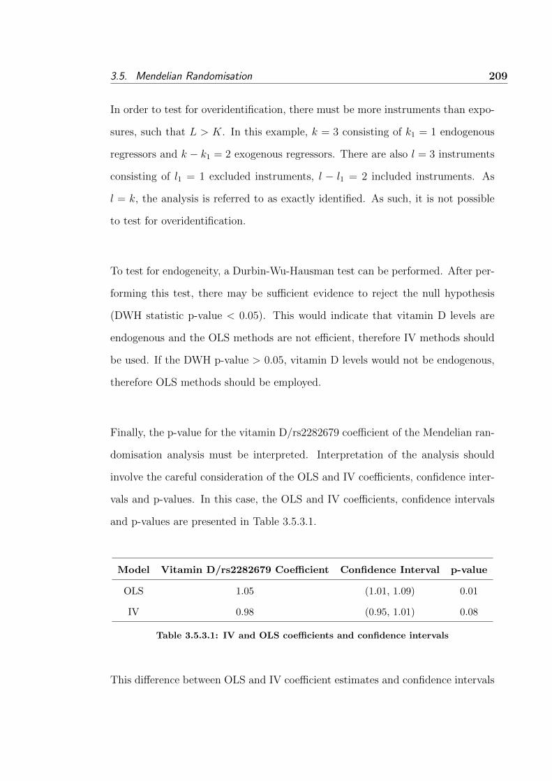
3.5. Mendelian Randomisation 209
In order to test for overidentification, there must be more instruments than expo-
sures, such that L > K. In this example, k = 3 consisting of k1 = 1 endogenous
regressors and k − k1 = 2 exogenous regressors. There are also l = 3 instruments
consisting of l1 = 1 excluded instruments, l − l1 = 2 included instruments. As
l = k, the analysis is referred to as exactly identified. As such, it is not possible
to test for overidentification.
To test for endogeneity, a Durbin-Wu-Hausman test can be performed. After per-
forming this test, there may be sufficient evidence to reject the null hypothesis
(DWH statistic p-value < 0.05). This would indicate that vitamin D levels are
endogenous and the OLS methods are not efficient, therefore IV methods should
be used. If the DWH p-value > 0.05, vitamin D levels would not be endogenous,
therefore OLS methods should be employed.
Finally, the p-value for the vitamin D/rs2282679 coefficient of the Mendelian ran-
domisation analysis must be interpreted. Interpretation of the analysis should
involve the careful consideration of the OLS and IV coefficients, confidence inter-
vals and p-values. In this case, the OLS and IV coefficients, confidence intervals
and p-values are presented in Table 3.5.3.1.
Model Vitamin D/rs2282679 Coefficient Confidence Interval p-value
OLS 1.05 (1.01, 1.09) 0.01
IV 0.98 (0.95, 1.01) 0.08
Table 3.5.3.1: IV and OLS coefficients and confidence intervals
This difference between OLS and IV coefficient estimates and confidence intervals
210Chapter 3. Mendelian Randomisation: An Application of Instrumental Variable
Techniques
(along with the DWH test) suggest that the observational epidemiological associ-
ation may be subject to bias. That is, that vitamin D levels may not be causally
associated with Breslow thickness and that the different OLS and IV estimates
may be due to unmeasured confounding or reverse causation. Therefore in this
situation, Mendelian randomisation analysis suggests that a public health inter-
vention to reduce the severity of melanoma by encouraging individuals to increase
their vitamin D levels through sun exposure or diet would not be beneficial.
3.5.4 Benefits of Mendelian randomisation
The use of genetic variants as excluded instruments in Mendelian randomisation
analysis has major advantages. It may help overcome the potential limitations of
observational epidemiological associations which were discussed in Section 3.3.2.1,
namely confounding, reverse causation, selection bias, and regression dilution.
3.5.4.1 Confounding
Exposures may be associated with socioeconomic, behavioural and lifestyle fac-
tors, however individual genetic variants are unlikely a priori to be associated
with these factors at a population level, due to their random transmission at con-
ception. This means that any reported association between a disease outcome and
the genetic variant will generally not be due to confounding.
3.5.4.2 Reverse causation
Presence of, and severity of disease may influence exposures in epidemiological
studies. This may be due to behavioural changes made by individuals, or through
unobserved chemical processes. However, genetic variants will not be influenced
by disease and will remain unchanged regardless of disease status.
3.5. Mendelian Randomisation 211
3.5.4.3 Selection bias
While individuals may be selected or volunteer for a study dependent on their
exposure and its influence on some disease measure, an individual is unlikely to
volunteer for or be selected either as a case or a control based solely on their
genetic variant.
3.5.4.4 Regression dilution bias
Unlike exposures, genetic variants only need to be measured once as they will
remain unchanged, and if these variants are associated with some exposure, the
genetic variant should be indicative of these exposure levels across the individual’s
lifetime.
3.5.5 Limitations of Mendelian randomisation
Along with the many advantages of Mendelian randomisation analysis, there
are several limitations [233, 243] which need to be considered when undertak-
ing Mendelian randomisation studies. The most significant of these, namely the
identification of a suitable genetic variant known with some certainty to be as-
sociated with the trait of interest, population stratification, and pleiotropy are
discussed in the following section.
3.5.5.1 Identification of suitable genetic variant for exposure
In order to use Mendelian randomisation, there must be a known genetic variant
that is clearly and consistently associated with the trait of interest [7]. Such a
variant may itself be directly functional or may be a marker in strong linkage
disequilibrium with one or more functional genetic variants. Historically, these
212Chapter 3. Mendelian Randomisation: An Application of Instrumental Variable
Techniques
variants have not been easy to identify, however with the increase in genome-wide
association studies and functional genomic work, more such genetic variants are
becoming available with each passing month [8, 243].
3.5.5.2 Reliable gene associations
As with any genetic epidemiological study, Mendelian randomisation studies re-
quire reliable associations between the genetic variant and exposure and also be-
tween the genetic variant and the disease outcome. Reliability of associations can
be determined by ensuring that the associations have been replicated in several
independent studies, and should also be confirmed within the current Mendelian
randomisation study [243]. However, genetic association studies are renowned
for producing statistical associations that are not able to be subsequently repli-
cated. In fact, an examination of 301 published studies of 25 different reported
associations found less than half of these associations had strong evidence of repli-
cation [259]. This lack of replication may be due to publication bias, small power
to detect associations and the reporting of spurious associations.
3.5.5.3 Population stratification
Population stratification occurs when a population consists of subgroups who have
systematic differences in disease rates and allele frequencies [224]. This can result
in associations between genetic variants and disease in the whole population which
are related to, and confounded, by ethnicity. This may result in confounding in a
Mendelian randomisation study, particularly when gene-exposure associations are
performed in different study populations to the gene-outcome associations.

3.5. Mendelian Randomisation 213
3.5.5.4 Pleiotropy
Mendelian randomisation analysis assumes that the genetic variant is associated
with the disease outcome only through the exposure. It is possible that this genetic
variant is pleiotropic and actually effects multiple traits. However, this is only a
problem if one of these additionally affected traits influence the outcome [243].
For example, in the vitamin D levels and Breslow thickness example discussed
earlier: if the rs2282679 SNP affects not only vitamin D levels, but also skin
pigmentation, then skin pigmentation may also affect Breslow thickness. This
would be violating the assumption (Section 3.4.2.1) that rs2282679 affects Breslow
thickness only through vitamin D levels. However, if rs2282679 is pleiotropic and
also affects height, it is unlikely that Breslow thickness will be affected by this.
3.5.6 Current software for Mendelian randomisation analysis
To the author’s knowledge, there are two software packages currently available
for Mendelian randomisation analysis; however neither were designed specifically
for use in the epidemiological framework. IVREG2 is a comprehensive module
for Stata which can perform Mendelian randomisation analysis using SNPs and
known haplotypes as the excluded instrument [242]. However, IVREG2 is only
able to use the most probable haplotype for each individual, which as discussed
in Section 3.5.2.2 may introduce bias. IVREG2 also performs comprehensive di-
agnostic tests described in Section 3.4.3 (please see page 199).
TSLS is a function in the R library sem [260] which, like IVREG2, can perform
Mendelian randomisation analysis using SNPs and the most probable haplotype
for each individual as excluded instruments. However, this function does not per-
214Chapter 3. Mendelian Randomisation: An Application of Instrumental Variable
Techniques
form any of the diagnostic tests described in Section 3.4.3, which are integral in
interpreting the results of the Mendelian randomisation analysis.
3.5.7 Software implementation
As there are no software packages available which model haplotype uncertainty in
Mendelian randomisation studies, the author designed a library within the soft-
ware package R [261], MRsnphap. MRsnphap has been designed to work within
the current SimHap [262] framework. SimHap is a statistical analysis program
designed to analyse associations between SNPs and haplotypes and various out-
comes. Two functions are available in MRsnphap – these are mrsnp.quant which
models Mendelian randomisation studies with the SNP as the excluded instru-
ment, and mrhap.quant which models these studies using phase-ambiguous hap-
lotypes. These functions also perform the testing described in Section 3.4.3, which
includes a test of overidentification, a test of endogeneity and an F-test for weak
instruments.
The methods employed in MRsnphap for Mendelian randomisation analyses are
described further in Sections 3.5.7.1 and 3.5.7.2 respectively.
3.5.7.1 Using SNPs as instruments: mrsnp.quant
The R function mrsnp.quant enables the user to perform Mendelian randomisa-
tion analysis, with a SNP as the excluded instrument. The mrsnp.quant function
is able to model continuous outcomes and exposures, while the SNP may be mod-
elled under additive, dominant or recessive assumptions, using a generalised linear

3.5. Mendelian Randomisation 215
model.
3.5.7.1.1 Example: mrsnp.quant
Referring back to the Mendelian randomisation example in Section 3.5.3 (please
see page 206), a researcher is interested in determining if there exists a causal
association between Breslow thickness and vitamin D levels. As they believe vita-
min D is an endogenous regressor, they use the rs2282679 SNP as an instrument
for vitamin D levels.
In order to use mrsnp.quant function, the MRsnphap library must be loaded.
When loading the MRsnphap library, several other libraries, including the SimHap
library are loaded simultaneously. In addition, the SimHap function SNP2Geno
must be used to generate the necessary SNP file. The code to load these pack-
ages, and run the necessary SimHap functions are included in the MRsnphap
manual in Appendix I.
The appropriate R input is:
mymodel < − mrsnp.quant(outcome = “BT”, exposure= “VitD”, covariates =
“AGE”, geneticmodel = “rs2282679 add”, geno=geno.dat, pheno=pheno.dat),
where BT (Breslow thickness) is a continuous outcome, VitD (vitamin D) is the
endogenous regressor and age is the exogenous regressor. The genetic model is
the rs2282679 SNP modelled additively, taking the values 0, 1 or 2, where these
indicate the number of variant alleles. The files containing the genotypic and

216Chapter 3. Mendelian Randomisation: An Application of Instrumental Variable
Techniques
phenotypic data are geno.dat and pheno.dat, respectively.
The output produced by mrsnp.quant can be seen in Appendix J.
3.5.7.2 Using haplotypes as instruments: mrhap.quant
The mrhap.quant function enables the user to perform Mendelian randomisa-
tion analysis, with a haplotype as the excluded instrument. Like mrsnp.quant,
mrhap.quant models continuous outcomes and exposures, and the haplotype can
be modelled as either additive, dominant or recessive. The mrhap.quant func-
tion uses the same maximum likelihood method as SimHap to infer diplotypes
for phase-ambiguous individuals; that is, for individuals whose diplotypes are not
known for certain. Each phase-ambiguous individual is assigned possible diplo-
types consisting of two haplotypes, where each haplotype has a probability at-
tached to it derived from the EM algorithm. This is because for phase-ambiguous
individuals, it is not clear which haplotypes each individual has within their diplo-
type. All that can be calculated (through the EM algorithm) is the probability of
an individual having certain haplotypes given their genotype set. As these hap-
lotypes occur with a probability and are not known for certain, this uncertainty
can be included within the modelling framework.
In SimHap, this is done by simulating data sets in which individuals are assigned
haplotypes with the appropriate probabilities. Particular statistical models are
then fitted to each simulated data set and the results are aggregated.
For example, in mrhap.quant, a Mendelian randomisation model is fitted to each

3.5. Mendelian Randomisation 217
simulated data set and coefficients and p-values for the Mendelian randomisa-
tion analysis are averaged. In addition, the mean F-statistic is presented for the
test for weak instruments, and the mean p-values are presented for the tests for
endogeneity and overidentification.
3.5.7.2.1 Example: mrhap.quant
The mrsnp.quant example described in Section 3.5.7.1.1 can be extended to in-
clude haplotypes in mrhap.quant. The researcher is interested in determining if
there exists a causal association between increased Breslow thickness and lower
vitamin D levels, and wishes to use a haplotype to test this. They choose a haplo-
type of several SNPs from the Vitamin D Receptor gene, CCTG, which has been
found to be associated with vitamin D levels.
As before, to use the mrhap.quant function, the MRsnphap library must first
be loaded. In addition, the SimHap functions SNP2Haplo, infer.haplos and
make.haplos must be used to generate the necessary haplotype files. The code
to load these packages, and run the necessary SimHap functions are included in
the MRsnphap manual in Appendix I.
The appropriate R input is:
mymodel < − mrhap.quant(outcome = “BT”, exposure= “VitD”, covariates
= “AGE”, geneticmodel = “CCTG”, haplo=myhaplo.dat, effect=“add”, sim=
1000, pheno=pheno.dat),

218Chapter 3. Mendelian Randomisation: An Application of Instrumental Variable
Techniques
where BT, VitD, and age are as described earlier. The genetic model is a haplo-
type modelled as an additive effect. In this example, the Mendelian randomisation
is simulated 1000 times. The files containing the haplotype and phenotypic data
are myhaplo.dat and pheno.dat, respectively.
The output produced by mrhap.quant can be seen in Appendix K.
3.5.8 Summary
This chapter has described an overview of epidemiological studies, and their failure
to identify causal associations between disease outcomes and modifiable exposures.
IV methods were proposed as a method to infer causality in epidemiological stud-
ies when the use of RCTs are not possible. An application of this technique –
Mendelian randomisation – was also proposed, and the benefits and limitations
of this technique were described. The remainder of this chapter described the
implementation of a novel extension to MR –the inclusion of imputed haplotypes
and the construction of an R library, MRsnphap, which performs Mendelian ran-
domisation using both SNPs and haplotypes as instruments.

219CHAPTER 4
Summary and Suggestions for Further Research
This final chapter provides a discussion of the findings of this thesis, and suggests
areas for further research.
This thesis has described the establishment of a population-based collection of
melanoma cases in Western Australia. The WAMHS facilitated investigation into
the genetic epidemiology of both melanoma susceptibility and prognosis. In addi-
tion, this thesis described the implementation of Mendelian randomisation tech-
niques in an R library, MRsnphap, which can be used to infer causal associations
in epidemiological studies.
4.1 The Western Australian Melanoma Health Study
The WAMHS was established with the aim of investigating the genetic epidemi-
ology of melanoma susceptibility and prognosis. The WAMHS is one the single
largest population-based studies of melanoma cases in the world, and the analysis
in this thesis has shown that the WAMHS is a valuable resource for investigating
genetic risk factors associated with melanoma susceptibility and progression.
The results of the association analyses between candidate genetic variants and
melanoma susceptibility replicated some of the associations identified by earlier
studies. However, not all associations were replicated in the WAMHS. This may
be due to one of four reasons: (1) the initial associations were spurious; (2) the
genetic variants associated with melanoma in other populations are not the same
as in the WAMHS; (3) the WAMHS sample (n=800) was underpowered to detect
these associations; or (4) the controls used in these analyses were not suitable. The

220 Chapter 4. Summary and Suggestions for Further Research
latter reason may be particularly relevant in the use of HapMap controls. Several
SNPs were also relatively rare (MAF < 0.15), which may have contributed to
low power as described in (3). As such, further investigation of these associations
in a larger WAMHS sample would help elucidate the potential role these genetic
variants have in melanoma susceptibility in the Western Australian population.
The analysis of Breslow thickness, as a surrogate for melanoma prognosis, pro-
vided evidence for novel associations between genetic variants and Breslow thick-
ness, which had not been widely studied previously. In particular, the current
study was the first of its kind to test the hypothesis that genetic variants which
predispose an individual to melanoma, are also associated with a poorer prog-
nosis. These associations, however, did not remain significant after adjustment
for multiple testing. This may have been due to two reasons: (1) the associa-
tions were spurious; or (2) this study had low statistical power to detect small
differences in Breslow thickness due to low MAF or small sample size (n=800).
As such, replication in larger samples is required. If the associations observed
in the current study are replicated, this may lead to an improved understanding
of the genetic mechanisms underlying both melanoma susceptibility and prognosis.
However, further studies should not be restricted only to testing associations be-
tween Breslow thickness and genetic variants which are associated with melanoma
susceptibility. While the analyses presented in this thesis provide some evidence
for the association of genetic variants with both increased melanoma susceptibility
and increased Breslow thickness, it is probable that other genetic variants exist
which affect only Breslow thickness. A GWAS of Breslow thickness would allow
an unbiased approach in identifying genetic variants associated with melanoma
4.2. Mendelian Randomisation 221
prognosis, however this would need to be performed on a large sample for suffi-
cient power.
The analyses presented in this thesis identified genetic variants which were associ-
ated with melanoma susceptibility and prognosis in the WAMHS. However, these
analyses had several limitations. The WAMHS sample consisted of only Western
Australian, adult, Caucasian individuals diagnosed with melanoma, and therefore
these results are generalisable only to Western Australian, adult, Caucasian indi-
viduals. In addition, the WAMHS sample used in this thesis was small (n=800),
therefore it would be preferable to attempt to replicate these associations in larger
samples. Furthermore, these analyses identified genetic variants associated with
melanoma susceptibility and prognosis, however these variants may not be causal,
and may only be markers for causal variants. Functional genetic investigations
are required to determine whether these associations are causal, and this may also
lead to an enhanced understanding of melanoma susceptibility and prognosis.
4.2 Mendelian Randomisation
Mendelian randomisation has been shown to overcome some of the problems with
observational epidemiological studies, by its ability to identify causal relationships.
The statistical methodological work to model imputed haplotypes in Mendelian
randomisation analyses is, to the best of my knowledge, novel. Prior to the imple-
mentation of Mendelian randomisation methods in the R library MRsnphap, to
the author’s knowledge, no software designed specifically for use in the setting of
genetic association analysis was available to perform these analyses. As such, the
uncertainty surrounding haplotype assignment had not previously been able to be
included in Mendelian randomisation analyses. The development of MRsnphap

222 Chapter 4. Summary and Suggestions for Further Research
will therefore allow researchers to perform Mendelian randomisation analyses us-
ing both SNPs and imputed haplotypes as instruments.
The MRsnphap library does have some limitations, and further development of
MRsnphap would make it more useful to epidemiological researchers. Possible
future developments of MRsnphap are described in the following section.
4.2.1 Future development of MRsnphap
In the current release of MRsnphap, the functions mrsnp.quant and mrhap.quant
assume conditional homoskedasticity of the errors. However, it is possible, partic-
ularly for family studies and longitudinal studies, that heteroskedasticity will be
present. As such, the methods described in Section 3.4.2 will no longer be valid;
the IV coefficient estimate will be unaffected by heteroskedasticity, however the
standard error estimates will be inconsistent [264] and therefore tests of statistical
significance will be invalid. Additionally, diagnostic tests, including the test for
endogeneity and overidentification will be affected.
Therefore, heteroskedasticity-consistent standard errors and statistics need to be
calculated. One method for this is Generalised Methods of Moments (GMM). In
fact, IV and OLS are special cases of GMM estimation. GMM is robust to het-
eroskedasticity, however its use does require very large samples [264]. Therefore,
a later release of MRsnphap could be developed to allow for both homoskedastic
and heteroskedastic errors, including the Pagan and Hall test [265] to determine
if heteroskedasticity is in fact present.

4.2. Mendelian Randomisation 223
Currently Mendelian randomisation analysis in MRsnphap requires the outcome
to be continuous, otherwise Assumption 4 in Section 3.4.2.1 will be violated. To
date, no methods have been published that allow the inclusion of binary outcomes,
however when available, these could be incorporated into MRsnphap. This would
allow for Mendelian randomisation analysis to determine causal associations be-
tween both binary and continuous measures of disease.
MRsnphap could also be extended to include imputed SNP data in Mendelian
randomisation studies that has been generated from GWAS. One commonly used
imputation program is IMPUTE [276]. After running the IMPUTE imputation
procedure, an output file is created which contains three probabilities for each
individual at each SNP. These probabilities represent the probability of each in-
dividual having each of the three genotypes, i.e. individual 1 at SNP A may have
the probabilities 0.2, 0.5, and 0.3 which represent the probability of having the
AG, GG, and GG genotypes, respectively. These probabilities could be used in
MRsnphap using the same modelling framework which is currently used for hap-
lotype analysis.
Some limitations of Mendelian randomisation described earlier in Section 3.5.5,
such as population stratification and pleiotropy, may be reduced by the use of
multiple instruments. That is, the use of two or more genetic variants which are
both associated with the exposure. At the current time, methods to incorporate
multiple genetic variants in Mendelian randomisation analysis are not available.
However, when available, these methods could be incorporated into MRsnphap.

224 Chapter 4. Summary and Suggestions for Further Research
4.3 Conclusion
The aims of this thesis, as described in Chapter 1, were to establish the WAMHS
database and to use these data to investigate the environmental, host and genetic
risk factors associated with melanoma susceptibility and prognosis. The main
hypothesis of these analyses was that factors associated with increased melanoma
susceptibility are also associated with poorer melanoma prognosis. One genetic
variant on the IRF4 gene was associated with both increased melanoma risk, and
thicker melanomas, resulting in a poorer melanoma prognosis.
In addition, this thesis aimed to extend a statistical technique for modelling causal
associations in epidemiological studies, known as Mendelian randomisation, to in-
clude the use of imputed haplotypes as instruments, and to implement this tech-
nique for use by other researchers in a library for R, MRsnphap.
The collection and use of high-quality genetic and epidemiological data is integral
in identifying risk factors for disease susceptibility and prognosis. The discovery
of genetic variants associated with melanoma susceptibility has the potential to
identify individuals who are high risk genetically of developing melanoma. These
identified individuals would then be able to modify their behaviour, for example,
by limiting their sun exposure, with the hope that the disease does not develop.
Similarly, the discovery of genetic variants associated with melanoma prognosis
may help identify individuals at increased risk of poorer melanoma prognosis,
and may also potentially lead to the development of new treatments. The de-
velopment of the R library MRsnphap may enable future melanoma (and other
disease) researchers to determine if environmental risk factors are causally asso-

4.3. Conclusion 225
ciated with disease. These lifestyle and behavioural risk factors for disease may
then be modified in order to reduce the impact of disease in the community.

226 Chapter 4. Summary and Suggestions for Further Research

227
Bibliography
[1] J.M. Last. A Dictionary of Epidemiology. Oxford University Press, 4th
edition, 2001.
[2] Hippocrates. On airs, waters, and places, 400 BC.
[3] J. Snow. The cholera near Golden Square, and at Deptford.
[4] W.G. Hill and B.S. Weir. Maximum-likelihood estimation of gene location
by linkage disequilibrium. American Journal of Human Genetics, 54:705–74,
1994.
[5] R. Doll and A.B. Hill. Smoking and carcinoma of the lung; preliminary
report. British Medical Journal, 2(4682):739–48, 1950.
[6] The Homocysteine Studies Collaboration. Homocysteine and risk of ischemic
heart disease and stroke. A meta-analysis. Journal of the American Medical
Association, 288:2015–22, 2002.
[7] S.J. Chanock, T. Manolio, M. Boehnke, E. Boerwinkle, D.J. Hunter, G.
Thomas, J.N Hirschhorn, G. Abecasis, D. Altshuler, J.E Bailey-Wilson, L.D
Brooks, L.R. Cardon, M. Daly, P. Donnelly, J.F Fraumeni, N.B Freimer,
D.S Gerhard, C. Gunter, A.E Guttmacher , M.S Guyer, E.L Harris, J.
Hoh, R. Hoover, C.A. Kong, K.R. Merikangas, C.C. Morton, L.J. Palmer,
E.G. Phimister, J.P. Rice, J. Roberts, C. Rotimi, M.A. Tucker, K.J. Vo-
gan, S. Wacholder, E.M Wijsman, D.M Winn, and F.S Collins. Replicating
genotype-phenotype associations Nature, 447(7145):655–60, 2007.

228 BIBLIOGRAPHY
[8] C.S. Ku, E.Y. Loy, Y. Pawitan, and K.S. Chia. The pursuit of genome-
wide association studies: where are we now? Journal of Human Genetics,
55(4):195–206, 2010.
[9] V. Didelez, and N. Sheehan. Mendelian randomization as an instrumen-
tal variable approach to causal inferences. Statistical Methods in Medical
Research, 16:309–30, 2007.
[10] H. Zur Hausen. Papillomaviruses in the causation of human cancers – a
brief historical account. Virology, 384(2):260–65, 2009.
[11] A.B. Hill. The environment and disease: Association or causation? Pro-
ceedings of the Royal Society of Medicine, 58:295–300, 1965.
[12] N.E. Morton. Outline of Genetic Epidemiology. Karger, Basel, 1982.
[13] D. Coggon, D. Barker, and G. Rose. Epidemiology for the Uninitiated. BMJ
Books, 2003.
[14] J.V. Neel and W.J. Schull. Human Heredity. University of Chicago Press,
Chicago, IL, 1954.
[15] M.J. Khoury. Genetic epidemiology and the future of disease prevention
and public health. Epidemiological Reviews, 19(1):175–80, 1997.
[16] H.L. Levy. Phenylketonuria: Old disease, new approach to treatment. Pro-
ceedings of the National Academy of Sciences of the United States of Amer-
ica, 96(5):1811–13, 1999.
[17] D. Wood, G. De Backer, O. Faergeman, I. Graham, G. Mancia, and K. Py-
orala. Prevention of coronary heart disease in clinical practice. European
Heart Journal, 19(10):1434–1503, 1998.

BIBLIOGRAPHY 229
[18] J. Bell. The new genetics: the new genetics in clinical practice. British
Medical Journal, 316(7131):618–20, 1998.
[19] R.H. Myers. Huntington’s disease genetics. Neurotherapeutics, 1(2):255–62,
2004.
[20] S.T. Lommatzsch and R. Aris. Genetics of cystic fibrosis. Seminars in
Respiratory and Critical Care Medicine, 30(5):531–38, 2009.
[21] W. Kalow. Pharmacogenetics and personalised medicine. Fundamental and
Clinical Pharmacology, 16(5):337–42, 2002.
[22] S. Mallal, D. Nolan, C. Witt, G. Masel, A.M. Martin, C. Moore, D. Sayer,
A. Castley, C. Mamotte, D. Maxwell, I. James, and F.T. Christiansen. As-
sociation between presence of HLA-B∗5701, HLA-DR7, and HLA-DQ3 and
hypersensitivity to HIV-1 reverse-transcriptase inhibitor abacavir. Lancet,
359(9308):727–32, 2002.
[23] S. Mallal, E. Phillips, G. Carosi, J.-M. Molina, C. Workman, J. Tomazic,
E. Jagel-Guedes, S. Rugina, O. Kozyrev, J.F. Cid, P. Hay, D. Nolan,
S. Hughes, A. Hughes, S. Ryan, N. Fitch, D. Thorborn, A. Benbow, and The
Predict-Study team. HLA-B∗5701 screening for hypersensitivity to abacavir.
New England Journal of Medicine, 358(6):568–79, 2008.
[24] L. Excoffier and M. Slatkin. Maximum-likelihood estimation of molecular
haplotype frequencies in a diploid population. Molecular Biology and Evo-
lution, 12(5):921–27, 1995.
[25] A.G. Clark. Inference of haplotypes from PCR-amplified samples of diploid
populations. Molecular Biology and Evolution, 7(2):111–22, 1990.

230 BIBLIOGRAPHY
[26] M. Stephens, N.J. Smith, and P. Donnelly. A new statistical method for hap-
lotype reconstruction from population data. American Journal of Human
Genetics, 68(4):978–89, 2001.
[27] T. Niu, Z.S. Qin, X. Xu, and J.S. Liu. Bayesian haplotype inference for mul-
tiple linked single-nucleotide polymorphisms. American Journal of Human
Genetics, 70(1):157–69, 2002.
[28] A. Gelman and T.P. Speed. Characterizing a joint probability distribution
by conditionals. Journal of the Royal Statistical Society. Series B (Method-
ological), 55(1):185–88, 1993.
[29] M.R. Cummings. Human Heredity:Principles and Issues. Wadsworth Pub-
lishing Company, 4th edition, 1997.
[30] A.A. Mitchell, D.J. Cutler, and A. Chakravarti. Undetected genotyping
errors cause apparent overtransmission of common alleles in the transmis-
sion/disequilibrium test. American Journal of Human Genetics, 72(3):598–
610, 2003.
[31] R.C. Lewontin. The interaction of selection and linkage. I. General consid-
erations; heterotic models. Genetics, 49(1):49–67, 1964.
[32] B.S. Kerem, J.M. Rommens, J.A. Buchanan, D. Markiewicz, T.K. Cox,
A. Chakravarti, M. Buchwald, and L.C. Tsui. Identification of the cystic-
fibrosis gene - genetic-analysis. Science, 245(4922):1073–80, 1989.
[33] M.E. Macdonald, C.M. Ambrose, M.P. Duyao, R.H. Myers, C. Lin,
L. Srinidhi, G. Barnes, S.A. Taylor, M. James, N. Groot, H. Macfar-
lane, B. Jenkins, M.A. Anderson, N.S. Wexler, J.F. Gusella, G.P. Bates,
S. Baxendale, H. Hummerich, S. Kirby, M. North, S. Youngman, R. Mott,
BIBLIOGRAPHY 231
G. Zehetner, Z. Sedlacek, A. Poustka, A.M. Frischauf, H. Lehrach, A.J.
Buckler, D. Church, L. Doucettestamm, M.C. Odonovan, L. Ribaramirez,
M. Shah, V.P. Stanton, S.A. Strobel, K.M. Draths, J.L. Wales, P. Dervan,
D.E. Housman, M. Altherr, R. Shiang, L. Thompson, T. Fielder, J.J. Was-
muth, D. Tagle, J. Valdes, L. Elmer, M. Allard, L. Castilla, M. Swaroop,
K. Blanchard, F.S. Collins, R. Snell, T. Holloway, K. Gillespie, N. Datson,
D. Shaw, and P.S. Harper. A novel gene containing a trinucleotide repeat
that is expanded and unstable on Huntington’s-disease chromosomes. Cell,
72(6):971–83, 1993.
[34] J.N. Hirschhorn and M.J. Daly. Genome-wide association studies for com-
mon diseases and complex traits. Nature Review Genetics, 6(2):95–108,
2005.
[35] J. Altmuller, L.J. Palmer, G. Fischer, H. Scherb, and M. Wjst. Genomewide
scans of complex human diseases: true linkage is hard to find. American
Journal of Human Genetics, 69(5):936–50, 2001.
[36] N. Risch and K. Merikangas. The future of genetic studies of complex human
diseases. Science, 273(5281):1516–17, 1996.
[37] Wellcome Trust Case Control Consortium. Genome-wide association study
of 14,000 cases of seven common diseases and 3,000 shared controls. Nature,
447(7145):661–78, 2007.
[38] R. Mayeux. Mapping the new frontier: complex genetic disorders. The
Journal of Clinical Investigation, 115(6):1404–07, 2005.
[39] A.T. Hattersley and M.I. McCarthy. What makes a good genetic association
study? Lancet, 366(9493):1315–23, 2005.
232 BIBLIOGRAPHY
[40] H.J. Cordell and D.G. Clayton. Genetic association studies. Lancet,
366(9491):1121–31, 2005.
[41] T.V. Perneger. What’s wrong with Bonferroni adjustments. BMJ,
316(7139):1236–38, 1998.
[42] Y. Benjamini and Y. Hochberg. Controlling the false discovery rate: a
practical and powerful approach to multiple testing. Journal of the Royal
Statistical Society, 57(1):289–300, 1995.
[43] J. Ferlay, F. Bray, P. Pisani, and D.M. Parkin. Globocan 2002: Cancer
incidence, mortality and prevalence worldwide, 2004.
[44] R. Laennec. Sur les melanoses. Bulletin de la Faculte de Medecine de Paris,
1:24–26, 1806.
[45] D.C. Bodenham. A study of 650 observed malignant melanomas in the
south-west region. Annals of the Royal College of Surgeons of England,
43(4):218–39, 1968.
[46] S. Cooper. First lines of theory and practice of surgery. Longman, Orme,
Brown, Green and Longman, London, 1840.
[47] M.J. Sladden, C. Balch, D.A. Barzilai, D. Berg, A. Freiman, T. Handiside,
S. Hollis, M.B. Lens, and J.F. Thompson. Surgical excision margins for
primary cutaneous melanoma. Cochrane Database of Systematic Reviews,
(4):CD004835, 2009.
[48] H.O. Lancaster. Some geographical aspects of the mortality from melanoma
in Europeans. Medical Journal of Australia, 43(26):1082–87, 1956.

BIBLIOGRAPHY 233
[49] J. Lin, T.L. Hocker, M. Singh, and H. Tsao. Genetics of melanoma predis-
position. British Journal of Dermatology, 159(2):286–91, 2008.
[50] M.P. Staples, M. Elwood, R.C. Burton, J.L. Williams, R. Marks, and G.G.
Giles. Non-melanoma skin cancer in Australia: the 2002 national survey
and trends since 1985. Medical Journal of Australia, 184(1):6–10, 2006.
[51] Australian Institute of Health, Welfare, and Australasian Association
of Cancer Registries. Cancer in Australia: an overview, 2008. Cancer series
no.046. AIHW, Canberra, 2008.
[52] Australian Institute of Health, Welfare, and Cancer Australia. Non-
melanoma skin cancer: general practice consultations, hospitalisation and
mortality. Technical Report Series no. 43. Cat. no. 39., Australian Institute
of Health and Welfare, 2008.
[53] Clark, W.H., D.E. Elder, D.T. Guerry, M.N. Epstein, M.H. Greene, and
M. Van Horn. A study of tumor progression: the precursor lesions of super-
ficial spreading and nodular melanoma. Human Pathology, 15(12):1147–65,
1984.
[54] A.J. Miller and M.C. Mihm. Mechanisms of disease - melanoma. New
England Journal of Medicine, 355(1):51–65, 2006.
[55] S.B. Gruber, R.L. Barnhill, K.S. Stenn, and G.C. Roush. Nevomelanocytic
proliferations in association with cutaneous malignant melanoma: a multi-
variate analysis. Journal of the American Academy of Dermatology, 21(4 Pt
1):773–80, 1989.
234 BIBLIOGRAPHY
[56] R. Marks, A.P. Dorevitch, and G. Mason. Do all melanomas come from
“moles”? a study of the histological association between melanocytic naevi
and melanoma. Australas Journal of Dermatology, 31(2):77–80, 1990.
[57] Y. Chudnovsky, P.A. Khavari, and A.E. Adams. Melanoma genetics and
the development of rational therapeutics. Journal of Clinical Investigation,
115(4):813–24, 2005.
[58] P. Jelfs, M. Coates, G. Giles, D. Shugg, T. Threlfall, D. Roder, I. Ring,
B. Shadbolt, and J. Condon. Cancer in Australia, 1989 to 1990 (with projec-
tions to 1995). Technical report, Australian Institute of Health and Welfare,
1996.
[59] Australian Institute of Health and Welfare. Australian Cancer Incidence
and Mortality. Australian Institute of Health and Welfare, Canberra, 2007.
[60] Australian Institute of Health and Welfare. Number of new cases and age-
specific rates for selected cancers by year of registration, sex and 5 year-age
groups. COGNOS data cube. Australian Institute of Health and Welfare,
Canberra, 2007.
[61] Australian Institute of Health, Welfare, Cancer Australia, and Aus-
tralasian Association of Cancer Registries. Cancer survival and prevalence
in Australia: cancers diagnosed from 1982 to 2004. Technical report, Aus-
tralian Institute of Health and Welfare, 2008.
[62] T. Threlfall and J. Thompson. Cancer incidence and mortality in Western
Australia, 2007. Technical report, Department of Health, 2009.
[63] T. Threlfall and J. Thompson. Cancer incidence and mortality in Western
Australia, 2005. Technical report, Department of Health, 2007.

BIBLIOGRAPHY 235
[64] T. Threlfall and J. Thompson. Cancer incidence and mortality in Western
Australia, 2006. Technical report, Department of Health, 2008.
[65] V. Bataille and E. De Vries. Melanoma–Part 1: Epidemiology, risk factors,
and prevention. British Medical Journal, 337:1287–91, 2008.
[66] S. Gandini, F. Sera, M.S. Cattaruzza, P. Pasquini, D. Abeni, P. Boyle,
and C.F. Melchi. Meta-analysis of risk factors for cutaneous melanoma:
I. Common and atypical naevi. European Journal of Cancer, 41(1):28–44,
2005.
[67] International Agency for Research on Cancer. IARC monograph on the
evaluation of carcinogenic risks to humans; ultraviolet radiation. Technical
report, 1992.
[68] Y. Chen and M. Berwick. Reproducibility of reported sun exposure be-
haviour in a case-control study of cutaneous malignant-melaoma. American
Journal of Epidemiology, 138(8):668–668, 1993.
[69] D.R. English, B.K. Armstrong, and A. Kricker. Reproducibility of reported
measurements of sun exposure in a case-control study. Cancer Epidemiology
Biomarkers & Prevention, 7(10):857–63, 1998.
[70] D.C. Whiteman, C.A. Whiteman, and A.C. Green. Childhood sun exposure
as a risk factor for melanoma: a systematic review of epidemiologic studies.
Cancer Causes & Control, 12(1):69–82, 2001.
[71] R. Steinitz, D.M. Parkin, J.L. Young, C.A. Bieber, and L. Katz. Cancer inci-
dence in Jewish migrants to Israel, 1961-1981. IARC Scientific Publications,
(98):1–311, 1989.

236 BIBLIOGRAPHY
[72] D. Anaise, R. Steinitz, and N.B. Hur. Solar-radiation - possible etiological
factor in malignant-melanoma in Israel - retrospective study (1960-1972).
Cancer, 42(1):299–304, 1978.
[73] M. Movshovi and B. Modan. Role of sun exposure in etiology of malignant-
melanoma - epidemiologic inference. Journal of the National Cancer Insti-
tute, 51(3):777–79, 1973.
[74] M. Khlat, A. Vail, M. Parkin, and A. Green. Mortality from melanoma
in migrants to Australia - variation by age at arrival and duration of stay.
American Journal of Epidemiology, 135(10):1103–13, 1992.
[75] A.J. Dobson and S.R. Leeder. Mortality from malignant-melanoma in Aus-
tralia - effects due to country of birth. International Journal of Epidemiol-
ogy, 11(3):207–11, 1982.
[76] M. McCredie, M.S. Coates, and J.M. Ford. Cancer incidence in European
migrants to New south Wales. Annals of Oncology, 1(3):219–25, 1990.
[77] C.D.J. Holman, C.D. Mulroney, and B.K. Armstrong. Epidemiology of
pre-invasive and invasive malignant-melanoma in Western Australia. Inter-
national Journal of Cancer, 25(3):317–23, 1980.
[78] A.J. McMichael and G.G. Giles. Cancer in migrants to Australia - extending
the descriptive epidemiological data. Cancer Research, 48(3):751–56, 1988.
[79] K.R. Cooke and J. Fraser. Migration and death from malignant-melanoma.
International Journal of Cancer, 36(2):175–78, 1985.
[80] R.S. Paffenbarger, A.L. Wing, and R.T. Hyde. Chronic diseases in for-
mer college-students. 15. Characteristics in youth predictive of adult-onset

BIBLIOGRAPHY 237
malignant-lymphomas, melanomas, and leukemias. Journal of the National
Cancer Institute, 60(1):89–92, 1978.
[81] L. Katz, S. Ben-Tuvia, and R. Steinitz. Malignant melanoma of the skin in
Israel: effect of migration. Trends in Cancer Incidence, Causes and Practical
Implications, 419–26, 1982.
[82] M.W. Hinds and L.N. Kolonel. Malignant-melanoma of the skin in Hawaii,
1960-1977. Cancer, 45(4):811–17, 1980.
[83] S. Gandini, F. Sera, M.S. Cattaruzza, P. Pasquini, O. Picconi, P. Boyle, and
C.F. Melchi. Meta-analysis of risk factors for cutaneous melanoma: II. Sun
exposure. European Journal of Cancer, 41(1):45–60, 2005.
[84] C.D.J. Holman, and B.K. Armstrong. Cutaneous malignant-melanoma and
indicators of total accumulated exposure to the sun - an analysis separating
histogenetic types. Journal of the National Cancer Institute, 73(1):75–82,
1984.
[85] A. Green, C. Bain, R. McLennan, and V. Siskind. Risk factors for cutaneous
melanoma in Queensland. Recent Results in Cancer Research, 102:76–97,
1986.
[86] J.M. Elwood. Melanoma and sun exposure - contrasts between intermittent
and chronic exposure. World Journal of Surgery, 16(2):157–65, 1992.
[87] C.D.J. Holman and B.K. Armstrong. Pigmentary traits, ethnic-origin,
benign nevi, and family history as risk-factors for cutaneous malignant-
melanoma. Journal of the National Cancer Institute, 72(2):257–66, 1984.

238 BIBLIOGRAPHY
[88] J.A.H. Lee and D. Strickland. Malignant-melanoma - social-status and out-
door work. British Journal of Cancer, 41(5):757–63, 1980.
[89] J.M. Bliss, D. Ford, A.J. Swerdlow, B.K. Armstrong, M. Cristofolini, J.M.
Elwood, A. Green, E.A. Holly, T. Mack, R.M. Mackie, A. Osterlind, S.D.
Walter, J. Peto, and D.F. Easton. Risk of cutaneous melanoma-associated
with pigmentation characteristics and freckling - systematic overview of 10
case-control studies. International Journal of Cancer, 62(4):367–76, 1995.
[90] B.K. Armstrong and A. Kricker. The epidemiology of UV induced skin
cancer. Journal of Photochemistry and Photobiology B: Biology, 63(1-3):8–
18, 2001.
[91] A.R. Rhodes, M.A. Weinstock, T.B. Fitzpatrick, M.C. Mihm, and A.J.
Sober. Risk-factors for cutaneous melanoma - a practical method of rec-
ognizing predisposed individuals. Journal of the American Medical Associ-
ation, 258(21):3146–54, 1987.
[92] T.R. Fears, C.C. Bird, D. Guerry, R.W. Sagebiel, M.H. Gail, D.E. Elder,
A. Halpern, E.A. Holly, P. Hartge, and M.A. Tucker. Average midrange
ultraviolet radiation flux and time outdoors predict melanoma risk. Cancer
Research, 62(14):3992–96, 2002.
[93] N.K. Hayward. Genetics of melanoma predisposition. Oncogene,
22(20):3053–62, 2003.
[94] A.W. Kopf, L.J. Hellman, G.S. Rogers, D.F. Gross, D.S. Rigel, R.J. Fried-
man, M. Levenstein, J. Brown, F.M. Golomb, and D.F. Roses. Familial ma-
lignant melanoma. Journal of the American Medical Association, 256:1915–
19, 1986.

BIBLIOGRAPHY 239
[95] S. Gandini, F. Sera, M.S. Cattaruzza, P. Pasquini, R. Zanetti, C. Masini,
P. Boyle, and C.F. Melchi. Meta-analysis of risk factors for cutaneous
melanoma: III. Family history, actinic damage and phenotypic factors. Eu-
ropean Journal of Cancer, 41(14):2040–59, 2005.
[96] D. Ford, J.M. Bliss, A.J. Swerdlow, B.K. Armstrong, S. Franceschi,
A. Green, E.A. Holly, T. Mack, R.M. Mackie, A. Osterlind. Risk of cu-
taneous melanoma associated with a family history of the disease. Interna-
tional Journal of Cancer, 62(4):377–81, 1995.
[97] R.L. Barnhill, G.C. Roush, L. Titus-Ernstoff, M.S. Ernstoff, P.H. Duray,
and J.M. Kirkwood. Comparison of nonfamilial and familial melanoma.
Dermatology, 184(1):2–7, 1992.
[98] M.A. Tucker and A.M. Goldstein. Melanoma etiology: where are we? Onco-
gene, 22(20):3042–52, 2003.
[99] J.A. Newton. Familial melanoma. Clinical and Experimental Dermatology,
18(1):5–11, 1993.
[100] V. Bataille, J.A.Newton–Bishop, P. Sasieni, A.J. Swerdlow, E. Pinney,
K. Griffiths, and J. Cuzickz. Risk of cutaneous melanoma in relation to
the numbers, types and sites of naevi: A case-control study. British Journal
of Cancer, 73(12):1605–11, 1996.
[101] M. Cristofolini, S. Franceschi, L. Tasin, G. Zumiani, F. Piscioli, R. Ta-
lamini, and C. Lavecchia. Risk-factors for cutaneous malignant-melanoma in
a northern Italian population. International Journal of Cancer, 39(2):150–
54, 1987.
240 BIBLIOGRAPHY
[102] P. Youl, J. Aitken, N. Hayward, D. Hogg, L. Liu, N. Lassam, N. Martin, and
A. Green. Melanoma in adolescents: A case-control study of risk factors in
Queensland, Australia. International Journal of Cancer, 98(1):92–98, 2002.
[103] C.J. Hussussian, J.P. Struewing, A.M. Goldstein, P.A.T. Higgins, D.S. Ally,
M.D. Sheahan, W.H. Clark, M.A. Tucker, and N.C. Dracopoli. Germline
p16 mutations in familial melanoma. Nature Genetics, 8(1):15–21, 1994.
[104] L. Zuo, J. Weger, Q. Yang, A.M. Goldstein, M.A. Tucker, G.J. Walker,
N. Hayward, and N.C. Dracopoli. Germline mutations in the p16INK4a
binding domain of CDK4 in familial melanoma. Nature Genetics, 12(1):97–
99, 1996.
[105] M. Falchi, V. Bataille, N.K. Hayward, D.L. Duffy, J.A.N. Bishop, T. Pasti-
nen, A. Cervino, Z.Z. Zhao, P. Deloukas, N. Soranzo, D.E. Elder, J.H.
Barrett, N.G. Martin, D.T. Bishop, G.W. Montgomery, and T.D. Spector.
Genome-wide association study identifies variants at 9p21 and 22q13 asso-
ciated with development of cutaneous nevi. Nature Genetics, 41(8):915–19,
2009.
[106] D.T. Bishop, F. Demenais, M.M. Iles, M. Harland, J.C. Taylor, E. Corda,
J. Randerson-Moor, J.F. Aitken, M.-F. Avril, E. Azizi, B. Bakker,
G. Bianchi-Scarra, B. Bressac-De Paillerets, D. Calista, L.A. Cannon-
Albright, T. Chin-a Woeng, T. Debniak, G. Galore-Haskel, P. Ghiorzo,
I. Gut, J. Hansson, M. Hocevar, V. Hoiom, J.L. Hopper, C. Ingvar, P.A.
Kanetsky, R.F. Kefford, M.T. Landi, J. Lang, J. Lubinski, R. Mackie,
J. Malvehy, G.J. Mann, N.G. Martin, G.W. Montgomery, F.A. Van Nieuw-
poort, S. Novakovic, H. Olsson, S. Puig, M. Weiss, W. Van Workum, D. Ze-
lenika, K.M. Brown, A.M. Goldstein, E.M. Gillanders, A. Boland, P. Galan,

BIBLIOGRAPHY 241
D.E. Elder, N.A. Gruis, N.K. Hayward, G.M. Lathrop, J.H. Barrett, and
J.A. Newton Bishop. Genome-wide association study identifies three loci
associated with melanoma risk. Nature Genetics, 41(8):920–25, 2009.
[107] K.M. Brown, S. MacGregor, G.W. Montgomery, D.W. Craig, Z.Z. Zhao,
K. Iyadurai, A. K Henders, N. Homer, M.J. Campbell, M. Stark, S. Thomas,
H. Schmid, E.A. Holland, E.M. Gillanders, D.L. Duffy, J.A. Maskiell, J. Je-
tann, M. Ferguson, D.A. Stephan, A.E. Cust, D. Whiteman, A. Green,
H. Olsson, S. Puig, P. Ghiorzo, J. Hansson, F. Demenais, A.M. Goldstein,
N.A. Gruis, D.E. Elder, J.N. Bishop, R.F. Kefford, G.G. Giles, B.K. Arm-
strong, J.F. Aitken, J.L. Hopper, N.G. Martin, J.M. Trent, G.J. Mann, and
N.K. Hayward. Common sequence variants on 20q11.22 confer melanoma
susceptibility. Nature Genetics, 40(7):838–40, 2008.
[108] D.F. Gudbjartsson, P. Sulem, S.N. Stacey, A.M. Goldstein, T. Rafnar,
B. Sigurgeirsson, K.R. Benediktsdottir, K. Thorisdottir, R. Ragnarsson,
S.G. Sveinsdottir, V. Magnusson, A. Lindblom, K. Kostulas, R. Botella-
Estrada, V. Soriano, P. Juberias, M. Grasa, B. Saez, R. Andres, D. Scherer,
P. Rudnai, E. Gurzau, K. Koppova, L.A. Kiemeney, M. Jakobsdottir,
S. Steinberg, A. Helgason, S. Gretarsdottir, M.A. Tucker, J.I. Mayordomo,
E. Nagore, R. Kumar, J. Hansson, J.H. Olafsson, J. Gulcher, A. Kong,
U. Thorsteinsdottir, and K. Stefansson. ASPI and TYR pigmentation vari-
ants associate with cutaneous melanoma and basal cell carcinoma. Nat
Genet, 40(7):886–91, 2008.
[109] P. Sulem, D.F. Gudbjartsson, S.N. Stacey, A. Helgason, T. Rafnar, K.P.
Magnusson, A. Manolescu, A. Karason, A. Palsson, G. Thorleifsson,
M. Jakobsdottir, S. Steinberg, S. Palsson, F. Jonasson, B. Sigurgeirsson,

242 BIBLIOGRAPHY
K. Thorisdottir, R. Ragnarsson, K.R. Benediktsdottir, K.K. Aben, L.A.
Kiemeney, J.H. Olafsson, J. Gulcher, A. Kong, U. Thorsteinsdottir, and
K. Stefansson. Genetic determinants of hair, eye and skin pigmentation in
Europeans. Nature Genetics, 39(12):1443–52, 2007.
[110] A. Kamb, D. Shattuck-Eidens, R. Eeles, Q. Liu, N.A. Gruis, W. Ding,
C. Hussey, T. Tran, Y. Miki, J. Weaver-Feldhaus, M. Mcclure, J.F. Aitken,
D.E. Anderson, W. Bergman, R. Frants, D.E. Goldgar, A. Green, R. Maclen-
nan, N.G. Martin, L.J. Meyer, P. Youl, J.J. Zone, M.H. Skolnick, and L.A.
Cannon-Albright. Analysis of the p16 gene (CDKN2) as a candidate for
the chromosome 9p melanoma susceptibility locus. Nat Genet, 8(1):22–26,
1994.
[111] A.M. Goldstein, M. Chan, M. Harland, N.K. Hayward, F. Demenais,
D. Timothy Bishop, E. Azizi, W. Bergman, G. Bianchi-Scarra, W. Bruno,
D. Calista, L.A. Cannon Albright, V. Chaudru, A. Chompret, F. Cuellar,
D.E. Elder, P. Ghiorzo, E.M. Gillanders, N.A. Gruis, J. Hansson, D. Hogg,
E.A. Holland, P.A. Kanetsky, R.F. Kefford, M. Teresa Landi, J. Lang, S.A.
Leachman, R.M. Mackie, V. Magnusson, G.J. Mann, J. Newton Bishop,
J.M. Palmer, S. Puig, J.A. Puig-Butille, M. Stark, H. Tsao, M.A. Tucker,
L. Whitaker, and E. Yakobson. Features associated with germline CDKN2A
mutations: a GenoMEL study of melanoma-prone families from three con-
tinents. Journal of Medical Genetics, 44(2):99–106, 2007.
[112] M. Berwick, I. Orlow, A.J. Hummer, B.K. Armstrong, A. Kricker, L.D.
Marrett, R.C. Millikan, S.B. Gruber, H. Anton-Culver, R. Zanetti, R.P.
Gallagher, T. Dwyer, T.R. Rebbeck, P.A. Kanetsky, K. Busam, L. From,
U. Mujumdar, H. Wilcox, and C.B. Begg. The prevalence of CDKN2A

BIBLIOGRAPHY 243
germ-line mutations and relative risk for cutaneous malignant melanoma:
An international population-based study. Cancer Epidemiology Biomarkers
& Prevention, 15(8):1520–25, 2006.
[113] D.T. Bishop, F. Demenais, A.M. Goldstein, W. Bergman, J.N. Bishop,
B. Bressac-De Paillerets, A. Chompret, P. Ghiorzo, N. Gruis, J. Hansson,
M. Harland, N. Hayward, E.A. Holland, G.J. Mann, M. Mantelli, D. Nancar-
row, A. Platz, and M.A. Tucker. Geographical variation in the penetrance
of CDKN2A mutations for melanoma. Journal of the National Cancer In-
stitute, 94(12):894–903, 2002.
[114] C.B. Begg, I. Orlow, A.J. Hummer, B.K. Armstrong, A. Kricker, L.D. Mar-
rett, R.C. Millikan, S.B. Gruber, H. Anton-Culver, R. Zanetti, R.P. Gal-
lagher, T. Dwyer, T.R. Rebbeck, N. Mitra, K. Busam, L. From, M. Berwick,
for the Genes Environment Melanoma Study Group. Lifetime risk of
melanoma in CDKN2A mutation carriers in a population-based sample.
Journal of the National Cancer Institute, 97(20):1507–15, 2005.
[115] J. Aitken, J. Welch, D. Duffy, A. Milligan, A. Green, N. Martin, and N. Hay-
ward. CDKN2A variants in a population-based sample of Queensland fami-
lies with melanoma. Journal of the National Cancer Institute, 91(5):446–52,
1999.
[116] N. Soufir, M.F. Avril, A. Chompret, F. Demenais, J. Bombled, A. Spatz,
D. Stoppa-Lyonnet, J. Benard, and B. Bressac-De Paillerets. Prevalence of
p16 and CDK4 germline mutations in 48 melanoma-prone families in France.
The French Familial Melanoma Study group. Human Molecular Genetics,
7(2):209–16, 1998.

244 BIBLIOGRAPHY
[117] A.M. Goldstein, J.P. Struewing, A. Chidambaram, M.C. Fraser, and M.A.
Tucker. Genotype-phenotype relationships in U.S. melanoma-prone fami-
lies with CDKN2A and CDK4 mutations. Journal of the National Cancer
Institute, 92(12):1006–10, 2000.
[118] A.M. Goldstein, A. Chidambaram, A. Halpern, E.A. Holly, D.I. Guerry,
R. Sagebiel, D.E. Elder, and M.A. Tucker. Rarity of CDK4 germline muta-
tions in familial melanoma. Melanoma Research, 12(1):51–55, 2002.
[119] P. Valverde, E. Healy, I. Jackson, J.L. Rees, and A.J. Thody. Variants of
the melanocyte-stimulating hormone receptor gene are associated with red
hair and fair skin in humans. Nature Genetics, 11(3):328–30, 1995.
[120] N.F. Box, J.R. Wyeth, L.E. O’Gorman, N.G. Martin, and R.A. Sturm.
Characterization of melanocyte stimulating hormone receptor variant alleles
in twins with red hair. Human Molecular Genetics, 6(11):1891–1897, 1997.
[121] J.S. Palmer, D.L. Duffy, N.F. Box, J.F. Aitken, L.E. O’Gorman, A.C. Green,
N.K. Hayward, N.G. Martin, and R.A. Sturm. Melanocortin-1 receptor
polymorphisms and risk of melanoma: Is the association explained solely by
pigmentation phenotype? American Journal of Human Genetics, 66(1):176–
86, 2000.
[122] P. Valverde, E. Healy, S. Sikkink, F. Haldane, A.J. Thody, A. Carothers,
I.J. Jackson, and J.L. Rees. The Asp84Glu variant of the melanocortin 1
receptor (MC1R) is associated with melanoma. Human Molecular Genetics,
5(10):1663–66, 1996.

BIBLIOGRAPHY 245
[123] S. Raimondi, F. Sera, S. Gandini, S. Iodice, S. Caini, P. Maisonneuve, and
M.C. Fargnoli. MC1R variants, melanoma and red hair color phenotype: A
meta-analysis. International Journal of Cancer, 122(12):2753–60, 2008.
[124] J. Han, P. Kraft, H. Nan, Q. Guo, C. Chen, A. Qureshi, S.E. Hankinson, F.B.
Hu, D.L. Duffy, Z.Z. Zhao, N.G. Martin, G.W. Montgomery, N.K. Hayward,
G. Thomas, R.N. Hoover, S. Chanock, and D.J. Hunter. A genome-wide
association study identifies novel alleles associated with hair color and skin
pigmentation. PLoS Genetics, 4(5):e1000074, 2008.
[125] C. Kennedy, J. Ter Huurne, M. Berkhout, N. Gruis, M. Bastiaens,
W. Bergman, R. Willemze, and J.N.B. Bavinck. Melanocortin 1 receptor
(MC1R) gene variants are associated with an increased risk for cutaneous
melanoma which is largely independent of skin type and hair color. Journal
of Investigative Dermatology, 117(2):294–300, 2001.
[126] N.F. Box, D.L. Duffy, W. Chen, M. Stark, N.G. Martin, R.A. Sturm, and
N.K. Hayward. MC1R genotype modifies risk of melanoma in families
segregating CDKN2A mutations. American Journal of Human Genetics,
69(4):765–73, 2001.
[127] A.M. Goldstein, M.T. Landi, S. Tsang, M.C. Fraser, D.J. Munroe, and M.A.
Tucker. Association of MC1R variants and risk of melanoma in melanoma-
prone families with CDKN2A mutations. Cancer Epidemiol Biomarkers &
Prevention, 14(9):2208–12, 2005.
[128] M. Shahbazi, V. Pravica, N. Nasreen, H. Fakhoury, A.A. Fryer, R.C.
Strange, P.E. Hutchinson, J.E. Osborne, J.T. Lear, A.G. Smith, and I.V.

246 BIBLIOGRAPHY
Hutchinson. Association between functional polymorphism in EGF gene
and malignant melanoma. Lancet, 359(9304):397–401, 2002.
[129] S.L. McCarron, A.C. Bateman, J.M. Theaker, and W.M. Howell. Egf +61
gene polymorphism and susceptibility to and prognostic markers in cuta-
neous malignant melanoma. International Journal of Cancer, 107(4):673–5,
2003.
[130] M.R. James, N.K. Hayward, T. Dumenil, G.W. Montgomery, N.G. Martin,
and D.L. Duffy. Epidermal growth factor gene (EGF) polymorphism and risk
of melanocytic neoplasia. Journal of Investigative Dermatology, 123(4):760–
2, 2004.
[131] J.A. Randerson-Moor, R. Gaut, F. Turner, L. Whitaker, J.H. Barrett,
I.D. Silva, A.J. Swerdlow, D.T. Bishop, and J.A.N. Bishop. The rela-
tionship between the epidermal growth factor (EGF) 5’ utr variant A61G
and melanoma/nevus susceptibility. Journal of Investigative Dermatology,
123(4):755–59, 2004.
[132] K.L. Amend, J.T. Elder, L.P. Tomsho, J.D. Bonner, T.M. Johnson,
J. Schwartz, M. Berwick, and S.B. Gruber. EGF gene polymorphism and
the risk of incident primary melanoma. Cancer Research, 64(8):2668–72,
2004.
[133] National Health and Medical Research Council. The management of cuta-
neous melanoma. Technical report, NHMRC, 1999.
[134] K.S. Smalley, N.K. Haass, P.A. Brafford, M. Lioni, K.T. Flaherty, and
M. Herlyn. Multiple signaling pathways must be targeted to overcome drug
BIBLIOGRAPHY 247
resistance in cell lines derived from melanoma metastases. Molecular Cancer
Therapeutics, 5(5):1136–44, 2006.
[135] A. Breslow. Thickness, cross-sectional areas and depth of invasion in prog-
nosis of cutaneous melanoma. Annals of Surgery, 172(5):902–8, 1970.
[136] A.C. Allen and S. Spitz. Malignant melanoma - a clinicopathological analysis
of the criteria for diagnosis and prognosis. Cancer, 6(1):1–45, 1953.
[137] C.M. Balch, J.E. Gershenwald, S.J. Soong, J.F. Thompson, M.B. Atkins,
D.R. Byrd, A.C. Buzaid, A.J. Cochran, D.G. Coit, S. Ding, A.M. Egger-
mont, K.T. Flaherty, P.A. Gimotty, J.M. Kirkwood, K.M. Mcmasters, Jr.
Mihm, M.C., D.L. Morton, M.I. Ross, A.J. Sober, and V.K. Sondak. Fi-
nal version of 2009 AJCC melanoma staging and classification. Journal of
Clinical Oncology, 27(36):6199–6206, 2009.
[138] R.L. Barnhill, J.A. Fine, G.C. Roush, and M. Berwick. Predicting five-year
outcome for patients with cutaneous melanoma in a population-based study.
Cancer, 78(3):427–32, 1996.
[139] C.M. Balch, S.J. Soong, J.E. Gershenwald, J.F. Thompson, D.S. Reintgen,
N. Cascinelli, M. Urist, K.M. Mcmasters, M.I. Ross, J.M. Kirkwood, M.B.
Atkins, J.A. Thompson, D.G. Coit, D. Byrd, R. Desmond, Y.T. Zhang, P.Y.
Liu, G.H. Lyman, and A. Morabito. Prognostic factors analysis of 17,600
melanoma patients: Validation of the American Joint Committee on Cancer
melanoma staging system. Journal of Clinical Oncology, 19(16):3622–34,
2001.
[140] C.M. Balch, T.M. Murad, S.J. Soong, A.L. Ingalls, N.B. Halpern, and W.A.
Maddox. A multifactorial analysis of melanoma: prognostic histopatholog-

248 BIBLIOGRAPHY
ical features comparing Clark’s and Breslow’s staging methods. Annals of
Surgery, 188(6):732–42, 1978.
[141] C. Garbe, P. Buttner, J. Bertz, G. Burg, B. D’hoedt, H. Drepper,
I. Guggenmoos-Holzmann, W. Lechner, A. Lippold, and C.E. Orfanos. Pri-
mary cutaneous melanoma. Identification of prognostic groups and estima-
tion of individual prognosis for 5093 patients. Cancer, 75(10):2484–91, 1995.
[142] N. Cascinelli, E. Marubini, A. Morabito, and R. Bufalino. Prognostic factors
for stage I melanoma of the skin: a review. Statistics in Medicine, 4(3):265–
78, 1985.
[143] K. Sondergaard and G. Schou. Survival with primary cutaneous malignant
melanoma, evaluated from 2012 cases. A multivariate regression analysis.
Virchows Archives: A. Pathological Anatomy & Histopathology, 406(2):179–
95, 1985.
[144] S. Retsas, K. Henry, M.Q. Mohammed, and K. Macrae. Prognostic factors
of cutaneous melanoma and a new staging system proposed by the American
Joint Committee on Cancer (AJCC): Validation in a cohort of 1284 patients.
European Journal of Cancer, 38(4):511–6, 2002.
[145] D.S. Rigel, G.S. Rogers, and R.J. Friedman. Prognosis of malignant
melanoma. Dermatologic Clinics, 3(2):309–14, 1985.
[146] C.M. Balch, S. Soong, M.I. Ross, M.M. Urist, C.P. Karakousis, W.J. Tem-
ple, M.C. Mihm, R.L. Barnhill, W.R. Jewell, H.J. Wanebo, and R. Harrison.
Long-term results of a multi-institutional randomized trial comparing prog-
nostic factors and surgical results for intermediate thickness melanomas (1.0

BIBLIOGRAPHY 249
to 4.0 mm). Intergroup Melanoma Surgical Trial. Annals of Surgical On-
cololgy, 7(2):87–97, 2000.
[147] P.J. Heenan, D.R. English, C. Darcy, J. Holman, and B.K. Armstrong. Sur-
vival among patients with clinical stage I cutaneous malignant-melanoma
diagnosed in Western Australia in 1975/1976 and 1980/1981. Cancer,
68(9):2079–87, 1991.
[148] A. Downing, X.Q. Yu, J. Newton-Bishop, and D. Forman. Trends in prog-
nostic factors and survival from cutaneous melanoma in Yorkshire, UK and
New South Wales, Australia between 1993 and 2003. International Journal
of Cancer, 123(4):861–66, 2008.
[149] H.J. Cohen, E. Cox, K. Manton, and M. Woodbury. Malignant-melanoma
in the elderly. Journal of Clinical Oncology, 5(1):100–106, 1987.
[150] P.J. Heenan and C.D.J. Holman. A histological comparison of cutaneous
malignant-melanoma between the Oxford region and Western Australia.
Histopathology, 6(6):703–16, 1982.
[151] P. Hersey, R.W. Sillar, C.G. Howe, R.C. Burton, S.V. Darbar, H.M. Foster,
S.M. Collins, D.E. Bradley, and D. Owens. Factors related to the presenta-
tion of patients with thick primary melanomas. Medical Journal of Australia,
154(9):583–87, 1991.
[152] J. Levine, A. Kopf, D. Rigel, R. Bart, P. Hennessey, R. Friedman, and
M. Mintzis. Correlation of thicknesses of superficial spreading malignant
melanomas and ages of patients. The Journal of Dermatologic Surgery and
Oncology, 7(4):311–16, 1981.

250 BIBLIOGRAPHY
[153] J.E. Osborne and P.E. Hutchinson. Clinical correlates of Breslow thickness
of malignant melanoma. British Journal of Dermatology, 144(3):476–83,
2001.
[154] L. Bucchi, M. Serafini, and G. Lanzanova. Breslow thickness of cuta-
neous malignant-melanoma in Ravenna (northern Italy) 1981-1990. Tumori,
78(2):94–97, 1992.
[155] J. Melia, E.J. Cooper, T. Frost, R. Grahambrown, J. Hunter, A. Marsden,
A. Duvivier, J. White, S. Whitehead, A.P. Warin, M. Wroughton, R. Ell-
man, and J. Chamberlain. Cancer-research campaign health-education pro-
gram to promote the early detection of cutaneous malignant-melanoma.
2.Characteristics and incidence of melanoma. British Journal of Dermatol-
ogy, 132(3):414–21, 1995.
[156] J.L. Schwartz, T.S. Wang, T.A. Hamilton, L. Lowe, V.K. Sondak, and T.M.
Johnson. Thin primary cutaneous melanomas: associated detection pat-
terns, lesion characteristics, and patient characteristics. Cancer, 95(7):1562–
8, 2002.
[157] D. Duke, J. Castresana, L. Lucchina, T.H. Lee, A.J. Sober, W.P. Carey, D.E.
Elder, and R.L. Barnhill. Familial cutaneous melanoma and two-mutational-
event modeling. Cancer, 72(11):3239–43, 1993.
[158] N.M. Fisher, J.V. Schaffer, M. Berwick, and J.L. Bolognia. Breslow depth of
cutaneous melanoma: Impact of factors related to surveillance of the skin,
including prior skin biopsies and family history of melanoma. Journal of the
American Academy of Dermatology, 53(3):393–406, 2005.
BIBLIOGRAPHY 251
[159] F. Grange, A. Chompret, M. Guilloud-Bataille, J.C. Guillaume, A. Mar-
gulis, M. Prade, F. Demenais, and M.F. Avril. Comparison between fa-
milial and nonfamilial melanoma in France. Archives of Dermatology,
131(10):1154–9, 1995.
[160] I. Okamoto, F. Roka, J. Krogler, G. Endler, S. Kaufmann, S. Tockner,
C. Marsik, B. Jilma, C. Mannhalter, O. Wagner, and H. Pehamberger.
The EGF A61G polymorphism is associated with disease-free period and
survival in malignant melanoma. Journal of Investigative Dermatology,
126(10):2242–46, 2006.
[161] T.B. Fitzpatrick. Soleil et peau. Journal of Medical Esthetics, 2:33–34, 1975.
[162] R.A. Fisher. On the interpretation of Chi2 from contingency tables, and the
calculation of p. Journal of the Royal Statistical Society, 85(1):87–94, 1922.
[163] D.C. Whiteman, M. Stickley, P. Watt, M.C. Hughes, M.B. Davis, and A.C.
Green. Anatomic site, sun exposure, and risk of cutaneous melanoma. Jour-
nal of Clinical Oncology, 24(19):3172–77, 2006.
[164] J.C. Barrett, B. Fry, J. Maller, and M.J. Daly. Haploview: analysis and
visualization of LD and haplotype maps. Bioinformatics, 21(2):263–5, 2005.
[165] B. Rhead, D. Karolchik, R.M. Kuhn, A.S. Hinrichs, A.S. Zweig, P.A. Fu-
jita, M. Diekhans, K.E. Smith, K.R. Rosenbloom, B.J. Raney, A. Pohl,
M. Pheasant, L.R. Meyer, K. Learned, F. Hsu, J. Hillman-Jackson, R.A.
Harte, B. Giardine, T.R. Dreszer, H. Clawson, G.P. Barber, D. Haussler,
and W.J. Kent. The UCSC genome browser database: update 2010. Nucleic
Acids Research, 38(Database issue):D613–9, 2010.
252 BIBLIOGRAPHY
[166] P.I. De Bakker, R. Yelensky, I. Pe’er, S.B. Gabriel, M.J. Daly, and D. Alt-
shuler. Efficiency and power in genetic association studies. Nature Genetics,
37(11):1217–23, 2005.
[167] P. Sulem, D.F. Gudbjartsson, S.N. Stacey, A. Helgason, T. Rafnar,
M. Jakobsdottir, S. Steinberg, S.A. Gudjonsson, A. Palsson, G. Thorleifsson,
S. Palsson, B. Sigurgeirsson, K. Thorisdottir, R. Ragnarsson, K.R. Benedik-
tsdottir, K.K. Aben, S.H. Vermeulen, A.M. Goldstein, M.A. Tucker, L.A.
Kiemeney, J.H. Olafsson, J. Gulcher, A. Kong, U. Thorsteinsdottir, and
K. Stefansson. Two newly identified genetic determinants of pigmentation
in Europeans. Nature Genetics, 40(7):835–7, 2008.
[168] D.L. Duffy, G.W. Montgomery, W. Chen, Z.Z. Zhao, L. Le, M.R. James,
N.K. Hayward, N.G. Martin, and R.A. Sturm. A three-single-nucleotide
polymorphism haplotype in intron 1 of OCA2 explains most human eye-
color variation. American Journal of Human Genetics, 80(2):241–52, 2007.
[169] T.R. Rebbeck, P.A. Kanetsky, A.H. Walker, R. Holmes, A.C. Halpern,
L.M. Schuchter, D.E. Elder, and D. Guerry. P gene as an inherited
biomarker of human eye color. Cancer Epidemiology Biomarkers & Pre-
vention, 11(8):782–84, 2002.
[170] R.A. Sturm, D.L. Duffy, Z.Z. Zhao, F.P. Leite, M.S. Stark, N.K. Hayward,
N.G. Martin, and G.W. Montgomery. A single SNP in an evolutionary
conserved region within intron 86 of the HERC2 gene determines human
blue-brown eye color. American Journal of Human Genetics, 82(2):424–31,
2008.

BIBLIOGRAPHY 253
[171] H. Eiberg, J. Troelsen, M. Nielsen, A. Mikkelsen, J. Mengel-from, K.W.
Kjaer, and L. Hansen. Blue eye color in humans may be caused by a per-
fectly associated founder mutation in a regulatory element located within
the HERC2 gene inhibiting OCA2 expression. Human Genetics, 123(2):177–
87, 2008.
[172] H. Shen, Z. Liu, S.S. Strom, M.R. Spitz, J.E. Lee, J.E. Gershenwald, M.I.
Ross, P.F. Mansfield, M. Duvic, H.N. Ananthaswamy, and Q. Wei. p53
codon 72 Arg homozygotes are associated with an increased risk of cutaneous
melanoma. Journal of Investigative Dermatology, 121(6):1510–4, 2003.
[173] Australian Bureau of Statistics. Population by age and sex, regions of Aus-
tralia, May 2008.
[174] W.C. Lee. Searching for disease-susceptibility loci by testing for Hardy-
Weinberg disequilibrium in a gene bank of affected individuals. American
Journal of Epidemiology, 158(5):397–400, 2003.
[175] International Hapmap Consortium. The international Hapmap project. Na-
ture, 426(6968):789–96, 2003.
[176] J. Stankovich, C.J. Cox, R.B. Tan, D.S. Montgomery, S.J. Huxtable, J.P.
Rubio, M.G. Ehm, L. Johnson, H. Butzkueven, T.J. Kilpatrick, T.P. Speed,
A.D. Roses, M. Bahlo, and S.J. Foote. On the utility of data from the
international Hapmap project for Australian association studies. Human
Genetics, 119(1-2):220–2, 2006.
[177] I.W. Webster. Editorial: Busselton, a community study in cardiovascular
disease. Australia & New Zealand Journal of Medicine, 4(4):412–4, 1974.

254 BIBLIOGRAPHY
[178] A.L. James, M.W. Knuiman, M.L. Divitini, J. Hui, M. Hunter, L.J. Palmer,
G. Maier, and A.W. Musk. Changes in the prevalence of asthma in adults
since 1966: the Busselton health study. European Respiratory Journal,
35(2):273–8, 2010.
[179] D.L. Duffy, Z.Z. Zhao, R.A. Sturm, N.K. Hayward, N.G. Martin, and G.W.
Montgomery. Multiple pigmentation gene polymorphisms account for a sub-
stantial proportion of risk of cutaneous malignant melanoma. Journal of
Investigative Dermatology, 130(2):520–8, 2010.
[180] P. Mccullagh and J. Nelder. Generalized Linear Models, Second Edition
(Chapman & Hall/CRC Monographs on Statistics & Applied Probability).
Chapman and Hall/CRC, 1989.
[181] W.J. Gauderman. Sample size requirements for association studies of gene-
gene interaction. American Journal of Epidemiology, 155(5):478–84, 2002.
[182] B.R. Cassileth, W.H. Clark, R.M. Heiberger, V. March, and A. Tenaglia.
Relationship between patients early recognition of melanoma and depth of
invasion. Cancer, 49(1):198–200, 1982.
[183] L. Temoshok, R.J. Diclemente, D.M. Sweet, M.S. Blois, and R.W. Sagebiel.
Factors related to patient delay in seeking medical attention for cutaneous
malignant-melanoma. Cancer, 54(12):3048–53, 1984.
[184] L. Temoshok, B.W. Heller, R.W. Sagebiel, M.S. Blois, D.M. Sweet, R.J.
Diclemente, and M.L. Gold. The relationship of psychosocial factors to
prognostic indicators in cutaneous malignant-melanoma. Journal of Psy-
chosomatic Research, 29(2):139–53, 1985.

BIBLIOGRAPHY 255
[185] J.E.J. Krige, S. Isaacs, D.A. Hudson, H.S. King, R.M. Strover, and C.A.
Johnson. Delay in the diagnosis of cutaneous malignant-melanoma - a
prospective-study in 250 patients. Cancer, 68(9):2064–68, 1991.
[186] M. Baccard, S. Chevret, P. Chemaly, and P. Morel. Delay in diagnosis of
melanoma. Prospective study in 102 patients. Annales De Dermatologie Et
De Venereologie, 124(9):601–606, 1997.
[187] M.A. Richard, J.J. Grob, M.F. Avril, M. Delaunay, X. Thirion, P. Wolken-
stein, P. Souteyrand, B. Dreno, J.J. Bonerandi, S. Dalac, L. Machet, J.C.
Guillaume, J. Chevrant-Breton, C. Vilmer, F. Aubin, B. Guillot, M. Beylot-
Barry, C. Lok, N. Raison-Peyron, and P. Chemaly. Melanoma and tu-
mor thickness - challenges of early diagnosis. Archives of Dermatology,
135(3):269–274, 1999.
[188] W. Liu, J.P. Dowling, W.K. Murray, G.A. Mcarthur, J.F. Thompson,
R. Wolfe, and J.W. Kelly. Rate of growth in melanomas - characteristics
and associations of rapidly growing melanomas. Archives of Dermatology,
142(12):1551–1558, 2006.
[189] Cancer Council Australia. Sunsmart : campaigns and events, October 2009.
[190] R.T. Vollmer and H.F. Seigler. Using a continuous transformation of the
Breslow thickness for prognosis in cutaneous melanoma. American Journal
of Clinical Pathology, 115(2):205–12, 2001.
[191] W. Stadelmann, D. Rapaport, S. Soong, D. Reintgen, A. Buzaid, and
C. Balch. Prognostic clinical and pathologic features. In C. Balch,
A. Houghton, A. Sober, and S. Soong, editors, Cutaneous Melanoma, vol-

256 BIBLIOGRAPHY
ume 3rd edition, pages 11–35. Quality Medical Publishing, Inc., St. Louis,
1998.
[192] E.K. Silverman and L.J. Palmer. Case-control association studies for the
genetics of complex respiratory diseases. American Journal of Respiratory
Cell & Molecular Biology, 22(6):645–8, 2000.
[193] C.B. Begg, A.J. Hummer, U. Mujumdar, B.K. Armstrong, A. Kricker, L.D.
Marrett, R.C. Millikan, S.B. Gruber, H.A. Culver, R. Zanetti, R.P. Gal-
lagher, T. Dwyer, T.R. Rebbeck, K. Busam, L. From, and M. Berwick. A
design for cancer case-control studies using only incident cases: experience
with the GEM study of melanoma. International Journal of Epidemiology,
35(3):756–64, 2006.
[194] E. De Vries, T.E.C. Nijsten, O. Visser, E. Bastiaannet, S. Van Hattem,
M.L. Janssen-Heijnen, and J.W.W. Coebergh. Superior survival of females
among 10,538 dutch melanoma patients is independent of Breslow thickness,
histologic type and tumor site. Annals of Oncology, 19(3):583–89, 2008.
[195] M. Berwick. Could sun exposure improve melanoma survival? Solar Radi-
ation and Human Health, page 95, 2008.
[196] K.B. Stitzenberg, N.E. Thomas, M. Berwick, H. Anton-Culver, U.J. Mu-
jumdar, and R.C. Millikan. Sociodemographic factors influencing Breslow
thickness at diagnosis for patients with melanoma. Journal of Clinical On-
cology (Meeting Abstracts), 25(18 suppl):6552–, 2007.
[197] P.F. Hanrahan, P. Hersey, and C.A. D’este. Factors involved in presenta-
tion of older people with thick melanoma. Medical Journal of Australia,
169(8):410–14, 1998.

BIBLIOGRAPHY 257
[198] A.J. Chamberlain, L. Fritschi, G.G. Giles, J.P. Dowling, and J.W. Kelly.
Nodular type and older age as the most significant associations of thick
melanoma in Victoria, Australia. Archives of Dermatology, 138(5):609–14,
2002.
[199] R.A. King and W.S. Oetting. Oculocutaneous albinism type 2. In R.P.
Pagon, T.C. Bird, T.C. Dolan, and K. Stephens, editors, GeneReviews.
University of Washington, Seattle, 2010/03/20 edition, 1993.
[200] W.S. Oetting and R.A. King. Molecular basis of albinism: mutations and
polymorphisms of pigmentation genes associated with albinism. Human
Mutation, 13(2):99–115, 1999.
[201] R.A. Sturm. Molecular genetics of human pigmentation diversity. Human
Molecular Genetics, 18(R1):R9–17, 2009.
[202] R.A. Sturm and M. Larsson. Genetics of human iris colour and patterns.
Pigment Cell Melanoma Research, 22(5):544–62, 2009.
[203] D.L. Duffy, N.F. Box, W. Chen, J.S. Palmer, G.W. Montgomery, M.R.
James, N.K. Hayward, N.G. Martin, and R.A. Sturm. Interactive effects of
MC1R and OCA2 on melanoma risk phenotypes. Human Molecular Genet-
ics, 13(4):447–61, 2004.
[204] K. Ryan, A. Phillips, and K. Vousden. Regulation and function of the p53
tumor suppressor protein. Current Opinion in Cell Biology, 13(3):332–37,
2001.
[205] T. Frebourg, N. Barbier, Y.X. Yan, J.E. Garber, M. Dreyfus, Jr. Fraumeni,
J., F.P. Li, and S.H. Friend. Germline p53 mutations in 15 families with Li-

258 BIBLIOGRAPHY
Fraumeni syndrome. American Journal of Human Genetics, 56(3):608–15,
1995.
[206] K.D. Gonzalez, K.A. Noltner, C.H. Buzin, D. Gu, C.Y. Wen-Fong, V.Q.
Nguyen, J.H. Han, K. Lowstuter, J. Longmate, S.S. Sommer, and J.N.
Weitzel. Beyond Li Fraumeni syndrome: Clinical characteristics of families
with p53 germline mutations. Journal of Clinical Oncology, 27(8):1250–56,
2009.
[207] I. Stefanaki, A.J. Stratigos, G. Dimisianos, V. Nikolaou, O. Papadopoulos,
D. Polydorou, H. Gogas, D. Tsoutsos, P. Panagiotou, E. Kanavakis, C. An-
toniou, and A.D. Katsambas. p53 codon 72 Pro homozygosity increases
the risk of cutaneous melanoma in individuals with dark skin complexion
and among noncarriers of melanocortin 1 receptor red hair variants. British
Journal of Dermatology, 156(2):357–62, 2007.
[208] J. Han, G. Cox, D., A. Colditz, G., and J. Hunter, D. The p53 codon 72
polymorphism, sunburns, and risk of skin cancer in US Caucasian women.
Molecular Carcinogenesis, 45(9):694–700, 2006.
[209] C. Li, K. Chen, Z. Liu, L.-E. Wang, J.E. Gershenwald, J.E. Lee, V.G. Prieto,
M. Duvic, E.A. Grimm, and Q. Wei. Polymorphisms of TP53 Arg72Pro, but
not p73 G4C14>A4TA4 and p21 Ser31Arg, contribute to risk of cutaneous
melanoma. Journal of Investigative Dermatology, 128(6):1585–88, 2007.
[210] M.R.A.-E. Hussein and G.S. Wood. Molecular aspects of melanocytic dys-
plastic nevi. Journal of Molecular Diagnostics, 4(2):71–80, 2002.
[211] G. Zhu, G.W. Montgomery, M.R. James, J.M. Trent, N.K. Hayward, N.G.
Martin, and D.L. Duffy. A genome-wide scan for naevus count: linkage to
BIBLIOGRAPHY 259
CDKN2A and to other chromosome regions. European Journal of Human
Genetics, 15(1):94–102, 2006.
[212] U. Sundram, J.D. Harvell, R.V. Rouse, and Y. Natkunam. Expression of the
B-cell proliferation marker MUM1 by melanocytic lesions and comparison
with S100, gp100 (HMB45), and melanA. Modern Pathology, 16(8):802–10,
2003.
[213] H. Davies, G.R. Bignell, C. Cox, P. Stephens, S. Edkins, S. Clegg, J. Teague,
H. Woffendin, M.J. Garnett, W. Bottomley, N. Davis, E. Dicks, R. Ew-
ing, Y. Floyd, K. Gray, S. Hall, R. Hawes, J. Hughes, V. Kosmidou,
A. Menzies, C. Mould, A. Parker, C. Stevens, S. Watt, S. Hooper, R. Wil-
son, H. Jayatilake, B.A. Gusterson, C. Cooper, J. Shipley, D. Hargrave,
K. Pritchard-Jones, N. Maitland, G. Chenevix-Trench, G.J. Riggins, D.D.
Bigner, G. Palmieri, A. Cossu, A. Flanagan, A. Nicholson, J.W. Ho, S.Y.
Leung, S.T. Yuen, B.L. Weber, H.F. Seigler, T.L. Darrow, H. Paterson,
R. Marais, C.J. Marshall, R. Wooster, M.R. Stratton, and P.A. Futreal.
Mutations of the BRAF gene in human cancer. Nature, 417(6892):949–54,
2002.
[214] P. Meyer, C. Sergi, and C. Garbe. Polymorphisms of the BRAF gene pre-
dispose males to malignant melanoma. Journal of Carcinogenesis, 2(1):7,
2003.
[215] S. Jackson, M. Harland, F. Turner, C. Taylor, P.A. Chambers, J. Randerson-
Moor, A.J. Swerdlow, I. Dos Santos Silva, S. Beswick, D.T. Bishop, and J.A.
Newton Bishop. No evidence for BRAF as a melanoma/nevus susceptibility
gene. Cancer Epidemiology, Biomarkers & Prevention, 14(4):913–8, 2005.

260 BIBLIOGRAPHY
[216] K. Laud, C. Kannengiesser, M.F. Avril, A. Chompret, D. Stoppa-Lyonnet,
L. Desjardins, A. Eychene, F. Demenais, G.M. Lenoir, and B. Bressac-
De Paillerets. BRAF as a melanoma susceptibility candidate gene? Cancer
Research, 63(12):3061–5, 2003.
[217] M. Shinozaki, A. Fujimoto, D.L. Morton, and D.S. Hoon. Incidence of braf
oncogene mutation and clinical relevance for primary cutaneous melanomas.
Clinical Cancer Research, 10(5):1753–7, 2004.
[218] S.C. Gorber, M. Tremblay, D. Moher, and B. Gorber. A comparison of
direct vs. self-report measures for assessing height, weight and body mass
index: a systematic review. Obesity Reviews, 8(4):307–26, 2007.
[219] I.A. Van Der Mei, L. Blizzard, A.L. Ponsonby, and T. Dwyer. Validity and
reliability of adult recall of past sun exposure in a case-control study of mul-
tiple sclerosis. Cancer Epidemiology, Biomarkers & Prevention, 15(8):1538–
44, 2006.
[220] L.K. Dennis, E. White, J.A. Lee, A. Kristal, B. Mcknight, and P. Odland.
Constitutional factors and sun exposure in relation to nevi: a population-
based cross-sectional study. American Journal of Epidemiology, 143(3):248–
56, 1996.
[221] M. Berwick and Y.T. Chen. Reliability of reported sunburn history in a
case-control study of cutaneous malignant melanoma. American Journal of
Epidemiology, 141(11):1033–7, 1995.
[222] M.A. Weinstock, G.A. Colditz, W.C. Willett, M.J. Stampfer, B. Rosner, and
F.E. Speizer. Recall (report) bias and reliability in the retrospective assess-

BIBLIOGRAPHY 261
ment of melanoma risk. American Journal of Epidemiology, 133(3):240–5,
1991.
[223] J. Mez, J. Cole, T. Howard, L. Macclellan, O. Stine, J. O’Connell, M. Woz-
niak, B. Stern, J. Sorkin, B. Mitchell, and S. Kittner. Evaluation of self-
reported ethnicity in a case-control population: the stroke prevention in
young women study. BMC Research Notes, 2(1):260, 2009.
[224] L.R. Cardon and L.J. Palmer. Population stratification and spurious allelic
association. Lancet, 361(9357):598–604, 2003.
[225] C.J. Mann. Observational research methods. research design. II: Cohort,
cross sectional, and case-control studies. Emergency Medical Journal,
20(1472-0205):54–60, 2003.
[226] R. Doll, R. Peto, J. Boreham, and I. Sutherland. Mortality in relation to
smoking: 50 years’ observations on male British doctors. British Medical
Journal, 328(7455):1519–28, 2004.
[227] R. Doll, R. Peto, J. Boreham, and I. Sutherland. Mortality from cancer
in relation to smoking: 50 years observations on British doctors. British
Journal of Cancer, 92(3):426–29, 2005.
[228] M.J. Stampfer and G.A. Colditz. Estrogen replacement therapy and coro-
nary heart-disease - a quantitative assessment of the epidemiologic evidence.
Preventive Medicine, 20(1):47–63, 1991.
[229] D. Grady, S.M. Rubin, D.B. Petitti, C.S. Fox, D. Black, B. Ettinger,
V.L. Ernster, and S.R. Cummings. Hormone-therapy to prevent disease
and prolong life in postmenopausal women. Annals of Internal Medicine,
117(12):1016–37, 1992.

262 BIBLIOGRAPHY
[230] D.A. Lawlor and G. Davey Smith. Cardiovascular risk and hormone replace-
ment therapy. Current Opinion in Obstetrics & Gynecology, 18(6):658–65,
2006.
[231] D.A. Lawlor, G. Davey Smith, K.R. Bruckdorfer, D. Kundu, and
S. Ebrahim. Those confounded vitamins: what can we learn from the dif-
ferences between observational versus randomised trial evidence? Lancet,
363(9422):1724–27, 2004.
[232] G. Davey Smith and S. Ebrahim. What can Mendelian randomisation tell
us about modifiable behavioural and environmental exposures? British
Medical Journal, 330(7499):1076–9, 2005.
[233] G. Davey Smith and S. Ebrahim. ‘Mendelian randomization’: can genetic
epidemiology contribute to understanding environmental determinants of
disease? International Journal of Epidemiology, 32(1):1–22, 2003.
[234] L.A. Bazzano, K. Reynolds, K.N. Holder, and J. He. Effect of folic acid
supplementation on risk of cardiovascular diseases - a meta-analysis of ran-
domized controlled trials. Journal of the American Medical Association,
296(22):2720–26, 2006.
[235] G. Davey Smith and S. Ebrahim. Mendelian randomization: prospects,
potentials, and limitations. International Journal of Epidemiology, 33(1):30–
42, 2004.
[236] D.A. Lawlor, G. Davey Smith, and S. Ebrahim. Socioeconomic position and
hormone replacement therapy use: explaining the discrepancy in evidence
from observational and randomized controlled trials. American Journal of
Public Health, 94(12):2149–54, 2004.

BIBLIOGRAPHY 263
[237] G. Davey Smith, Y. Ben-Shlomo, and J. Lynch. Life course approaches to
inequalities in coronary heart disease risk. In S.A. Stansfeld, M.G. Mar-
mot, editors, Stress and the heart. Psychosocial pathways to coronary heart
disease. BMJ Books, London, 2002.
[238] M.J. Thun, R. Peto, A.D. Lopez, J.H. Monaco, S.J. Henley, C.W. Heath,
and R. Doll. Alcohol consumption and mortality among middle-aged and
elderly US adults. New England Journal of Medicine, 337(24):1705–14, 1997.
[239] S. Ebrahim and G. Davey Smith. Mendelian randomization: can genetic epi-
demiology help redress the failures of observational epidemiology? Human
Genetics, 123(1):15–33, 2008.
[240] S. Macmahon, R. Peto, R. Collins, J. Godwin, S. Macmahon, J. Cutler,
P. Sorlie, R. Abbott, R. Collins, J. Neaton, R. Abbott, A. Dyer, and J. Stam-
ler. Blood pressure, stroke, and coronary heart disease : Part 1, prolonged
differences in blood pressure: prospective observational studies corrected for
the regression dilution bias. The Lancet, 335(8692):765–74, 1990.
[241] G. Davey Smith and A.N. Phillips. Inflation in epidemiology: “the proof and
measurement of association between two things” revisited. British Medical
Journal, 312(7047):1659–61, 1996.
[242] M. E. Baum, C.A.S. and S. Stillman. IVREG2: Stata module for extended
instrumental variables/2SLS and GMM estimation, 2002. Statistical Soft-
ware Components.
[243] D.A. Lawlor, R.M. Harbord, J.A. Sterne, N. Timpson, and G. Davey Smith.
Mendelian randomization: Using genes as instruments for making causal
inferences in epidemiology. Statistics in Medicine, 27(8):1133–63, 2007.

264 BIBLIOGRAPHY
[244] D. Staiger and J.H. Stock. Instrumental variables regression with weak
instruments. Econometrica, 65(3):557–86, 1997.
[245] J.D. Sargan. The estimation of economic relationships using instrumental
variables. Econometrica, 26(3):393–415, 1958.
[246] J.M. Wooldridge. Introductory Econometrics: A Modern Approach. Thom-
son Learning, New York, 2nd edition, 2003.
[247] J. Durbin. Errors in variables. Review of the International Statistical Insti-
tute, 22:23–32, 1954.
[248] D.M. Wu. Alternative tests of independence between stochastic regressors
and disturbances. Econometrica, 41(4):733–50, 1973.
[249] J. Hausman. Specication tests in econometrics. Econometrica, 46(3):1251–
71, 1978.
[250] M.B. Katan. Apolipoprotein-E isoforms, serum-cholesterol, and cancer, Mar
1986.
[251] S. Trompet, J.W. Jukema, M.B. Katan, G.J. Blauw, N. Sattar, B. Buckley,
M. Caslake, I. Ford, J. Shepherd, R.G. Westendorp, and A.J. De Craen.
Apolipoprotein E genotype, plasma cholesterol, and cancer: a Mendelian
randomization study. Am J Epidemiol, 170(11):1415–21, 2009.
[252] K.H. Allin, B.G. Nordestgaard, J. Zacho, A. Tybjaerg-Hansen, and S.E. Bo-
jesen. C-reactive protein and the risk of cancer: a Mendelian randomization
study. Journal of the National Cancer Institute, 102(3):202–6, 2010.
BIBLIOGRAPHY 265
[253] S.J. Lewis. Mendelian randomization as applied to coronary heart disease,
including recent advances incorporating new technology. Circulation: Car-
diovascular Genetics, 3(1):109–17, 2010.
[254] G. Pare and S.S. Anand. Mendelian randomisation, triglycerides, and CHD.
Lancet, 375(9726):1584–6, 2010.
[255] J. Danesh and M.B. Pepys. C-reactive protein and coronary disease: is there
a causal link? Circulation, 120(21):2036–9, 2009.
[256] A. Ioannidis, E. Ikonomi, N.L. Dimou, L. Douma, and P.G. Bagos. Poly-
morphisms of the insulin receptor and the insulin receptor substrates genes
in polycystic ovary syndrome: a Mendelian randomization meta-analysis.
Molecular Genetics & Metabolism, 99(2):174–83, 2010.
[257] N.J. Timpson, D.A. Lawlor, R.M. Harbord, T.R. Gaunt, I.N.M. Day, L.J.
Palmer, A.T. Hattersley, S. Ebrahim, G.D.O. Lowe, A. Rumley, and G.
Davey Smith. C-reactive protein and its role in metabolic syndrome:
Mendelian randomisation study. Lancet, 366(9501):1954–59, 2005.
[258] P.A. Mccaskie, G. Cadby, J. Hung, B.M. Mcquillan, C.M. Chapman, K.W.
Carter, P.L. Thompson, L.J. Palmer, and J.P. Beilby. The C-480T hepatic
lipase polymorphism is associated with HDL-C but not with risk of coronary
heart disease. Clinical Genetics, 70(2):114–21, 2006.
[259] K.E. Lohmueller, C.L. Pearce, M. Pike, E.S. Lander, and J.N. Hirschhorn.
Meta-analysis of genetic association studies supports a contribution of
common variants to susceptibility to common disease. Nature Genetics,
33(2):177–82, 2003.
[260] J. Fox. SEM: Structural equation models, 2009.

266 BIBLIOGRAPHY
[261] R Development Core Team. R: A Language and Environment for Statistical
Computing. Vienna, 2005.
[262] K.W. Carter, P.A. Mccaskie, and L.J. Palmer. SimHap GUI: an intuitive
graphical user interface for genetic association analysis. BMC Bioinformat-
ics, 9:557, 2008.
[263] J.A. Newton-Bishop, S. Beswick, J. Randerson-Moor, Y.M. Chang, P. Af-
fleck, F. Elliott, M. Chan, S. Leake, B. Karpavicius, S. Haynes, K. Kukalizch,
L. Whitaker, S. Jackson, E. Gerry, C. Nolan, C. Bertram, J. Marsden, D.E.
Elder, J.H. Barrett, and D.T. Bishop. Serum 25-hydroxyvitamin d3 lev-
els are associated with Breslow thickness at presentation and survival from
melanoma. Journal of Clinical Oncology, 27(32):5439–44, 2009.
[264] F. Hayashi. Econometrics. Princeton University Press, Princeton, 1st edi-
tion, 2000.
[265] A.R. Pagan and A.D. Hall. Diagnostic tests as residual analysis. Economet-
ric Reviews, 2(2):159–218, 1983.
[266] Y. Li and G.R. Abecasis. MACH 1.0: rapid haplotype reconstruction
and missing genotype inference. American Journal of Human Genetics,
S79:2290, 2006.
[267] P.I.W. de Bakker, M.A.R. Ferreira, X. Jia, B.M. Neale, S. Raychaudhuri,
and B.F. Voight. Practical aspects of imputation-driven meta-analysis of
genome-wide association studies. Human Molecular Genetics, 17(2):R122-
R128, 2008.
[268] J.H. Stock, J.H. Wright, and M. Yogo. A Survey of Weak Instruments and
Weak Identification in Generalized Method of Moments. American Statisti-

BIBLIOGRAPHY 267
cal Association Journal of Business and Economic Statistics, 20(4):518-529,
2002.
[269] D.L. Duffy, M.M. Iles, D. Glass, G. Zhu, J.H. Barrett, V. Hoiom, Z.Z Zhao,
R.A. Sturm, N. Soranzo, C. Hammond, M. Kvaskoff, D.C. Whiteman, M.
Mangino, J. Hansson, J.A. Newton-Bishop, GenoMEL, V. Bataille, N.K.
Hayward, N.G. Martin, D.T. Bishop, T.D. Spector, and G.W. Montgomery.
IRF4 variants have age-specific effects on nevus count and predispose to
melanoma. American Journal of Human Genetics, 87(1):6-16, 2010.
[270] K. Lasithiotakis, U. Leiter, F. Meier, T. Eigentler, G. Metzler, M. Moehrle,
H. Breuninger, and C. Garbe. Age and gender are significant independent
predictors of survival in primary cutaneous melanoma. Cancer, 112(8):1795-
804, 2008.
[271] C.R Scoggins, M.I. Ross, D.S. Reintgen, R.D. Noyes, J.S. Goydos, P.D.
Beitsch, M.M. Urist, S. Ariyan, J.J. Sussman, M.J. Edwards, A.B. Chag-
par, R.C. Martin, A.J. Stromberg, L. Hagendoorn, and K.M. McMasters.
Gender-related differences in outcome for melanoma patients. Annals of
Surgery, 243(5):693-8, 2006.
[272] N.G. Williams and T.M. Roberts. Signal transduction pathways involving
the raf proto-oncogene. Cancer and Metastasis Reviews, 13(1):105, 1994.
[273] Office for National Statistics. Mortality Statistics: Cause. England and
Wales 2008. London TSO, 2010.
[274] R.W. Morris and N.L. Kaplan. On the advantage of haplotype analysis in
the presence of multiple disease susceptibility alleles. Genetic Epidemiology,
23(3):221-223,2002.
268 BIBLIOGRAPHY
[275] P.S. Rosenberg, A. Che, and B.E. Chen. Multiple hypothesis testing strate-
gies for genetic case-control association studies. Statistics in Medicine,
25(18):3134-3149, 2006.
[276] B.N. Howie, P. Donnelly, and J. Marchini. A flexible and accurate geno-
type imputation method for the next generation of genome-wide association
studies. PLoS Genetics, 5(6):e1000529, 2009.
[277] M.F. Holick. Vitamin D Deficiency. New England Journal of Medicine,
357:266-281, 2007.
[278] J. Ahn, D. Albanes, S.I. Berndt, U. Peters, N. Chatterjee, N.D. Freed-
man, C.C. Abnet, W.Y. Huang, A.S. Kibel, E.D.Crawford, S.J. Weinstein,
S.J. Chanock, A. Schatzkin, and R.B. Hayes. Vitamin D-related genes,
serum vitamin D concentrations and prostate cancer risk. Carcinogenesis,
30(5):769776, 2009.
[279] J. Bound, D.A. Jaeger, and R.M. Baker. Problems with instrumental vari-
ables estimation when the correlation between the instruments and the en-
dogenous explanatory variable is weak. Journal of the American Statistical
Association, 90(430):443-450, 1995.
[280] R.P. Gallagher, D.I. McLean, C.P. Yang, A.J. Coldman, H.K.B. Silver,
J.J. Spinelli, and M. Beagrie. Suntan, Sunburn, and Pigmentation Fac-
tors and the Frequency of Acquired Melanocytic Nevi in Children. Similar-
ities to Melanoma: The Vancouver Mole Study Archives of Dermatology,
126(6):770-776, 1990.

BIBLIOGRAPHY 269
[281] M.P. Staples, M. Elwood, R.C. Burton, J.L. Williams, R. Marks, and G.G
Giles. Non-melanoma skin cancer in Australia: the 2002 national survey and
trends since 1985 Medical Journal of Australia, 184(1):6-10, 2006.

270 BIBLIOGRAPHY

271APPENDIX A
Letter to Doctor

Western Australian Cancer Registry Information Collection and Management, DOH (WA)
1st floor C Block, 189 Royal St EAST PERTH WA 6004
Ph. 08 9222 4022 Fax 08 9222 4236 Website: http://www.health.wa.gov.au/wacr
e-mail: [email protected]
«DOCNAME» «Doctor_Mail_Add1» «Doctor_Mail_Add2» «Doctor_Mail_Add3» «Doctor_Mail_Town» «Doctor_Mail_PCode»
Dear Dr «DOCSNAM»
I am writing to you about the Western Australian Melanoma Health Study (WAMHS) which has recently been established in order to develop a database of information and blood specimens to assist in research into this disease, which has significant mortality and morbidity.
The researchers wish to approach persons diagnosed with melanoma, via the Western Australian Cancer Registry (WACR), to seek their consent and participation. Participation involves the patient completing a questionnaire containing health and lifestyle information, as well as donating a blood sample for storage and use in medical research.
I am attaching details of persons whom WACR information suggests were your patients. I would appreciate it if you would indicate on the list whether there is any reason not to approach particular people about this project and return it to us in the reply paid envelope provided. If we do not receive a reply from you within four weeks, we will assume that you have no concerns about the researchers contacting any of the people listed.
Should you have any questions or would like further information about the WACR, please do not hesitate to contact me using the details above. For more information about the Study, please contact the WAMHS study coordinator, Ms Sarah Ward, on (08) 9346 1119.
This study has been approved by The University of Western Australia Ethics Committee and the Confidentiality of Health Information Committee of the Department of Health.
Yours sincerely,
Dr Timothy Threlfall Principal Medical Officer/Manager
<<Date>>

273APPENDIX B
Doctor Information Sheet
1
WESTERN AUSTRALIAN MELANOMA
HEALTH STUDY
Information for Doctors
BACKGROUND AND PURPOSE
Researchers from the Centre for Genetic Epidemiology and Biostatistics at The University of Western Australia have established the Western Australian Melanoma Health Study (WAMHS) in an effort to investigate the genetic and environmental factors that may cause malignant melanoma. This study has been approved by the University of Western Australia’s Human Research Ethics Committee and the Department of Health’s Human Research Ethics Committee (formerly Confidentiality of Health Information Committee).
Your patient/s are being asked to take part in this study because they have recently been diagnosed with melanoma, and have had this noted in the Western Australian Cancer Registry (WACR). We are asking all patients who have been diagnosed with melanoma in Western Australia to consider participating in this study.
Taking part in this study is completely voluntary. This information sheet will give you information regarding the study that your patient/s are being invited to participate in.
WHAT DO YOU HAVE TO DO?
You are asked to indicate on the enclosed list of your patients that have been diagnosed with malignant melanoma, if there is any reason, medical or other, not to approach particular patients about this project. You are then asked to return the list to the WACR in the reply paid envelope provided. Those patients that you consider suitable to participate in the study will be contacted by the WACR and can then decide if they wish to participate.
How will consent be handled? Once approval to contact the patient has been indicated by you, information about the WAMHS and a consent form will be sent directly to them by the WACR, on behalf of the WAMHS research staff. They will have ample time to discuss their decision with you, their family or WAMHS research staff and will be asked to return the consent form indicating their decision either way to the WACR. If the patient consents to participate in the study, the WACR will notify the WAMHS research staff.
WHAT IS THE PATIENT GIVING CONSENT FOR?
If patients choose to take part in the study, they will be asked to:
• Complete a questionnaire: This would involve the patient answering questions on their health, lifestyle, background and family history. The questionnaire will be conducted as a telephone interview and will take approximately 45 minutes.
• Provide a blood sample: This would be collected for serum and DNA at a PathWest collection centre, with the option of providing an additional sample for RNA.
2
• Health information access: In addition we will ask for consent to access health information kept about the patient. This information may come from hospital case notes, GP records or may be information kept about them by the Department of Health as part of its regular function.
DOES THE PATIENT HAVE TO TAKE PART IN THE STUDY?
No. Participation in this study is entirely up to the individual and their care will not be affected in any way by their decision. We will not inform you as the treating doctor whether your patient chose to participate. Patients can also withdraw their consent at any time by communicating this to WAMHS staff in writing.
WHO CAN ANSWER QUESTIONS ABOUT THE STUDY?
If you or your patients have any concerns or questions about the Western Australian Melanoma Health Study, please contact the WAMHS staff:
Website: http://www.wamhs.org.au
Phone: (08) 6488 6753 or 1800 145 511 (Sarah Ward - Study Coordinator)
Mail: Western Australian Melanoma Health Study Centre for Genetic Epidemiology and Biostatistics
The University of Western Australia M409, 35 Stirling Highway CRAWLEY WA 6009
OTHER ISSUES
If you or your patients have any queries about the Western Australian Cancer Registry, please contact the registry directly:
Mail: Dr. Timothy Threlfall Principal Medical Officer and Manager Western Australia Cancer Registry Department of Health (WA) 1st Floor C Block, 189 Royal Street East Perth WA 6004
Phone: (08) 9222 4022
If you or your patients have any complaints about any aspect of the study, or any questions about your patients’ rights as participants, then you may contact this committee:
Mail: Secretary, Human Research Ethics Committee Registrar’s Office - University of Western Australia 35 Stirling Highway Crawley WA 6009
Phone: (08) 6488 3703

275APPENDIX C
Letter to Patient
«crn»
Western Australian Cancer Registry Information Collection and Management, DOH (WA)
1st floor C Block, 189 Royal St EAST PERTH WA 6004
Ph. 08 9222 4022 Fax 08 9222 4236 Website: http://www.health.wa.gov.au/wacr
e-mail: [email protected]
«title» «FORENAME1» «FORENAME2» «SURNAME» «Person_Mail_Address» «Person_Mail_Town» WA «Person_Mail_PostCode»
Dear «title» «SURNAME» I am writing to ask for your assistance in an important state wide research project, interested in identifying the factors that cause malignant melanoma. This study is called the Western Australian Melanoma Health Study (WAMHS), and is being conducted by researchers at the Centre for Genetic Epidemiology and Biostatistics at The University of Western Australia. Currently, melanoma is the third most common form of cancer in Australia. The researchers wish to collect a blood sample and information on health, lifestyle and family history from people recently diagnosed with melanoma. Please find an information brochure about the study enclosed. Your name has been notified to the Western Australian Cancer Registry (WACR) as a result of medical tests, as required by law, and I am writing to invite you to participate in this study (please also find an information brochure about the WACR enclosed). If we could identify your doctor, we have contacted them as a courtesy prior to writing to you. However, your doctor will not be notified as to whether you chose to participate in this study or not. Further, no personal information will be given to any researchers without your consent. If you would like to participate in this study, I would be grateful if you would read and complete the enclosed consent form and post it back to me, using the reply paid envelope provided. No stamp is required (free postage). An extra copy of the consent form is also enclosed for you to keep for your records. If you do agree to participate, I will forward your name and consent to the WAMHS team at the Centre for Genetic Epidemiology and Biostatistics. They will then send you a questionnaire and a blood collection form to take with you if you have a blood sample taken. I will send a reminder letter about this study in 2 weeks, as it is most important to the success of the research that we get information from everyone we contact about whether they want to take part or not. If you do NOT wish to participate, you can indicate this on the consent form, so I can avoid sending you another letter and your name will NOT be given to the researchers. I appreciate your time in considering this request, and would be happy to discuss any problems or other WACR matters with you. Alternatively, you can call the Study Coordinator, Ms Sarah Ward, on 1800 145 511 (free-call number) or (08) 9346 1119 about the study itself. Yours sincerely,
Dr Timothy Threlfall Principal Medical Officer/Manager
«DATE»

277APPENDIX D
Patient Information Brochure

Participant Information Brochure
What is the purpose of this study?
Researchers at the Centre for Genetic Epidemiology and Biostatistics
(CGEB) at the University of Western Australia are investigating why people get malignant melanoma, a type of skin cancer, as part of the Western
Australian Melanoma Health Study (WAMHS).
Causes of melanoma include genetic (hereditary factors passed on to you
from your parents) and environmental factors (such as lifestyle differences
between people).
You are being asked to take part in this study because you have recently
been diagnosed with melanoma, and this has been notified to the Western Australian Cancer Registry (WACR). All patients who have been diagnosed
with malignant melanoma in Western Australia are being asked if they would
like to be a part of this study.
This information brochure will give you information to help you decide
whether or not you would like to be a part of the study. Please read this
carefully and discuss with members of your family and friends, as necessary.
Do I have to take part in this study?
No. Taking part in this study is completely voluntary and entirely up to you. Your decision will not be revealed to your doctor and will not affect your care
in any way.
What does this study involve?
There are three parts to this study:
1. Questionnaire (necessary)
2. Blood samples (two options)
a. One type of blood sample (DNA and serum)
b. Two types of blood samples (DNA, serum and RNA)
3. Health information access
You may participate in one part, more than one part, or all parts. However, if you participate in any parts of the study, you will need to
complete the questionnaire (Part 1) so that researchers can better
understand any environmental factors that are relevant to you.
1
Part 1. Questionnaire
What is this for?
The questionnaire provides information about your health and lifestyle, your
background and family history, and your melanoma. This information will help
us to understand environmental factors that cause melanoma.
What does this involve?
The questionnaire will be completed in a telephone interview with WAMHS
staff at a time convenient to you. This should take approximately 45 minutes.
Before the interview, some questions will be sent to you, so that you can
complete them beforehand (e.g. height) and have the answers ready to give
the interviewer.
What will be done with this information?
This information will be used by medical researchers interested in
environmental or lifestyle factors which may be involved in melanoma, e.g.
sun exposure. In addition, information regarding your family history will help
to see if melanoma runs in families.
Part 2. Blood Samples
What is this for?
Blood samples are very important to help in understanding malignant
melanoma. Specifically, blood samples can be used to identify possible
causes, improve diagnosis and potentially lead to new treatments. Your
sample will greatly assist melanoma research in the following ways:
1. A number of blood tests are currently performed to detect certain types
of disease, such as the cholesterol test for high cholesterol or the blood
sugar test for diabetes.
New tests are currently being developed for other forms of skin cancer
(basal cell carcinoma (BCC) and squamous cell carcinoma (SCC)). Your
blood sample would be very valuable in helping to evaluate new tests
that may be able to be used for melanoma.
2. Genes or DNA carry the information in your body that determines many
2
of your characteristics, including the colour of your hair or eyes. RNA is
produced from genes and in turn makes all the proteins in your body.
Your DNA and RNA will be used in research looking at the genes that
affect melanoma.
Some researchers may wish to perform tests to see if you are carrying
genes that might predict risk of melanoma or that may be involved in
whether or not you respond to a particular type of therapy.
What does this involve?
There are two options for the type of blood sample that you can donate:
a. One type of blood sample (DNA and serum)
This blood sample will provide a sample of your DNA (along with serum - the
proteins and chemicals in your blood).
If you would only like to donate this blood sample, it can be collected at any
PathWest centre in Western Australia (both metropolitan and regional
centres).
You will be asked to give approximately 30ml (about 2 and a half
tablespoons) of blood with this option.
b. Two types of blood samples (DNA, serum and RNA)
An extra blood sample is needed to collect RNA. This is collected at the
same time as the sample for DNA and serum, as part of the same blood test.
As a special tube is used to collect the RNA, it can only be done at certain
PathWest centres.
If you would like to donate both types of blood samples, this will be collected
at the PathWest centre at QEII Medical Centre in Nedlands, Perth.
You will be asked to give approximately 35ml (about 3 tablespoons) of blood
with this option.
What will be done with this information?
Serum, DNA and RNA will be extracted from your blood sample and stored in
small plastic tubes in a secure freezer located at the Western Australian DNA
Bank (WADB), within the CGEB.
3

The samples will be used by medical researchers in biochemical and genetic
studies of melanoma and other types of skin cancer such as basal cell
carcinoma (BCC) and squamous cell carcinoma (SCC).
These types of skin cancer occur more often than melanoma but are not as
dangerous, as they are less likely to spread to other parts of the body or
spread as quickly. All three types of skin cancer develop in different types of
cells in the skin and differ in their appearance.
Your blood will not be used for research that involves reproductive
cloning. Researchers will not be permitted to work out a genetic profile of
you as an individual.
With your permission, we would like to store this blood indefinitely for future
research into skin cancer. As such, your blood will be stored until it has all
been used, unless you contact the WAMHS to request its destruction
(contact details on the back page of this brochure).
What are the future implications of donating blood?
Feedback to participants
Your donated samples are not intended to be used in your diagnosis or
treatment. Feedback will not normally be given to participants regarding
personal genetic information. This is because melanoma is not thought to
be caused by just one gene (e.g. like cystic fibrosis is), but a complex
disease with many genes contributing to its development.
These genes will have small effects by themselves for each individual and
will generally combine together with other factors (such as other genes, the
environment, or lifestyle factors) to increase disease risk.
The disease risk attributable to each factor will be small and we do not yet
know exactly how all these elements interact, so releasing genetic
information would not be clinically meaningful or useful to you or your family.
However, it is possible that future DNA testing may result in new information
about diseases or potential diseases that you carry. Such information will
require extensive testing and validation before it can be determined to be
clinically useful but some of this information may have health implications for
yourself and your family, including your descendants.
4
Contact with you about any potentially important findings will only be made
where there is clear evidence of the medical importance to you or your
family. Each situation will be carefully reviewed by a Human Research Ethics
Committee before you are informed of the availability of results.
At that time, you may choose whether you would like to receive information
and what further information and tests you would like to proceed with.
Information will be provided through approved medical channels. Please note
it is your responsibility to keep the WAMHS up to date with your contact
details.
Disclosure to family members
You should consider whether or not any significant health information
obtained as a result of DNA testing should be disclosed to your family
members or descendents in the future. We will ask whether you consent to
the disclosure of your information to your family members or descendents (on
the attached consent form).
Family members would have to supply a written request to the Chief
Investigator and a Human Research Ethics Committee would review and
consider the request to disclose information.
Part 3. Health Information Access
What is this for?
The discovery of factors important in understanding disease may also require
additional knowledge of other relevant medical information about you,
beyond what is already stored in the WACR in the Department of Health of
Western Australia .
What does this involve?
We will ask for your consent for the WAMHS to access medical information
kept about you that is relevant to medical research, for example specific
information about other illnesses you may have had in the past. This
information may come from hospital case notes, GP records or from the
Department of Health as part of its routine data collection.
What will be done with this information?
This information will be used for research into melanoma and related health
areas.
5

281APPENDIX E
Patient Consent Form

1
WESTERN AUSTRALIAN MELANOMA HEALTH STUDY
CONSENT FORM I have read the information given to me and have had all of my questions answered. I have also been given a copy of the:
• Information Brochure entitled “DNA (Genetic) Testing and Storing”;
• Patient Information Brochure for the Western Australian Melanoma Health Study and
• Consent Form for my records
There are 8 parts to this consent form, Parts A to H. If you WOULD LIKE to participate in the WA Melanoma Health Study, please complete parts A to H of this consent form including completing and signing the declaration in Part H. You may consent to any or all parts of the study. However, it is necessary to consent to participate in the questionnaire (Part A) in order to consent to participate in the other parts. If you WOULD NOT LIKE to participate in the WA Melanoma Health Study, please go straight to Part H: Declaration, tick the box stating that you do not agree to participate and sign the form.
Part A: Consent to participate in questionnaire
I consent to complete a questionnaire about the lifestyle and environmental factors associated with melanoma. The questionnaire will be completed by phone interview at a time convenient to me. Some questions will be mailed to me before the interview, so that I can complete them beforehand and have the answers ready at the time of the interview (e.g. height).
I Do Do Not (Please continue below) (Please go to Part H)
Part B: Consent for Blood Sample and Storage for Medical Research
I consent to blood being taken and donate that blood absolutely for testing and research into melanoma and related health areas. In making my donation of blood, I understand and agree that: (a) the blood (which in this consent form includes its constituents and any genetic material or any
cell lines derived from the blood) will be stored and used for research into melanoma and related health areas;
(b) storage of blood samples will be conducted in accordance with the National Health & Medical Research Council’s1* Guidelines for Genetic Registers and Associated Genetic Material. Storage will be conducted under a coded system, to ensure that my confidentiality is maintained;
(c) samples of blood held will be discarded upon my written request;
1 *The National Health & Medical Research Council advises the Australian community and Commonwealth and the
State Governments on standards of individual and public health, and supports research to improve these standards.
2
(d) access to my blood donation for research will be managed by an Advisory Committee and only released where the research project that wishes to use my blood donation has been approved by a Human Research Ethics Committee;
(e) feedback will not normally be given to me regarding my personal genetic research information as these results would not be clinically meaningful or useful to me;
(f) I can ask to know more specific details of any studies that used my blood sample by contacting the WA Melanoma Health Study;
(g) the results of the research may be of interest to my immediate family, including my descendants, and I may decide whether or not the information may be disclosed to my family in accordance with ‘Options for disclosure to family members’ detailed in Part C;
(h) international research collaborations using my blood will only take place where researchers abide by equal or more stringent regulations of privacy and ethics as those in Australia, as assessed by a Human Research Ethics Committee;
(i) the Chief Investigator of this project and his or her associates involved with this project as well as The University of Western Australia will not be liable for any loss or damage to the blood/tissue taken or used in accordance with this form.
I consent to the collection of a blood sample for DNA extraction and biochemical analyses (from serum) and understand that this donation is given under the conditions (a) to (i) stated above. I understand that this sample may be taken at any PathWest centre in WA.
I Do Do Not (Please continue below) (Please go to Part C)
IN ADDITION:
I also consent to the collection of an additional blood sample for RNA to be taken at the same time as the sample for DNA and serum is collected. I understand that this donation is also given under the conditions (a) to (i) stated above. I understand that this sample must be taken at the QE-II Medical Centre, Nedlands.
I Do Do Not (Please go to Part C) (Please go to Part C)
Part C: Options for disclosure to family members
Please only complete this section if you have consented to any part of Part B.
I understand that future DNA testing may result in new information about diseases or potential diseases that may have health implications for my family, including my descendants. I understand that extensive testing and validation would be required before the information can be determined to be useful and that information can only be provided through approved medical channels when there is clear evidence of the medical importance to my family.
I consent to genetic information obtained from my DNA, as a result of this study, being revealed to my family members, upon their written request to the Chief Investigator, in the event of my death.
I Do Do Not (Please go to Part D) (Please go to Part D)
N.B: Part D is no longer applicable
3
Part E: Consent to access health information
I consent to allow access to health information about me relevant to melanoma-related research, such as is kept in a medical record or by the WA Department of Health, to assist medical research only where the research proposal has been approved by a Human Research Ethics Committee.
I Do Do Not (Please go to Part F) (Please go to Part F)
Part F: Future clinical trials for new treatments for melanoma
I consent to allow WAMHS staff to contact me in the future if there are any new treatments for melanoma which I may be suitable for (for example a clinical trial for a new drug or other treatment).
I Do Do Not (Please go to Part G) (Please go to Part G)
Part G: General
I understand that: (a) If a researcher wishes to obtain additional information or samples from me, my name will not be
divulged to that researcher without my written permission; (b) Any research results about me, and the fact that I have taken part in this study, will not be
revealed to any third party without my written consent, except if required by law; (c) The researchers will not reveal my identity and personal information about this project if
published in any public form; (d) I will not receive, or be entitled to, any reward or remuneration for providing my blood sample for
this project. I understand that the sample being donated could be used for commercial development and acknowledge the public interest in the research and donate the sample absolutely;
(e) I understand the potential benefits and risks involved in taking part in this study which have been
explained to me and I accept the risks involved. I have had the opportunity to ask questions and am satisfied with the explanation and the answers to my questions;
(f) I may withdraw from the study at any time, no questions asked, and without it negatively
affecting my future medical treatment; (g) If I choose to withdraw from the study, I understand that any information about me already
collected by the researchers will be retained unless I request otherwise in writing; (h) I understand that my information will only be collected and used for the study of melanoma and
related conditions. Related conditions are defined as other types of skin cancer; basal cell carcinoma (BCC) and squamous cell carcinoma (SCC).
4
Part H: Declaration
(Please tick the option that applies)
I agree to participate in the WA Melanoma Health Study and consent to the parts of the study that I have indicated in Part A through F. I have also read and understood Part G.
OR
I do not agree to participate in the WA Melanoma Health Study. Please sign:
……………………………... …………...………… …………………...
Name of Participant Signature Date ……………………………... …………...………… …………………...
Name of Witness Signature Date
The Human Research Ethics Committee at The University of Western Australia requires that all participants are informed that, if they have any complaint regarding the manner in which a research project is conducted, it may be given to the researcher or, alternatively, to the Secretary, Human Research Ethics Committee, Registrar’s Office, The University of Western Australia, Nedlands, WA 6009 (telephone number 6488-3703, fax number 6488-3861, email [email protected]). Name:
Address: CRN:

5
IF YOU HAVE CONSENTED TO PARTICIPATE
PLEASE COMPLETE THE FOLLOWING:
QUESTIONNAIRE INTERVIEW TIMES The questionnaire part of the study is completed by telephone interview. Could you please place a √ next to the day you would prefer us to call you for this interview?
Monday Tuesday Wednesday Thursday Friday
Could you please place a √ next to the time you would prefer us to call you for this interview:
Morning (9am-12pm) Afternoon (12pm-5pm) Evening (5pm – 8pm)
We will try to contact you on your home number first to complete the interview. If we are unable to contact you on this number, could you please place a √ next to the phone number you would prefer us to try contacting you on.
Work phone Mobile
CONTACT DETAILS
Please complete the following details: Home Phone Number Work Phone Number
Mobile Number
Please check the following details that we have for you and amend any that are incorrect. Name: Address: Date of Birth:

285APPENDIX F
Mole-Counting Chart
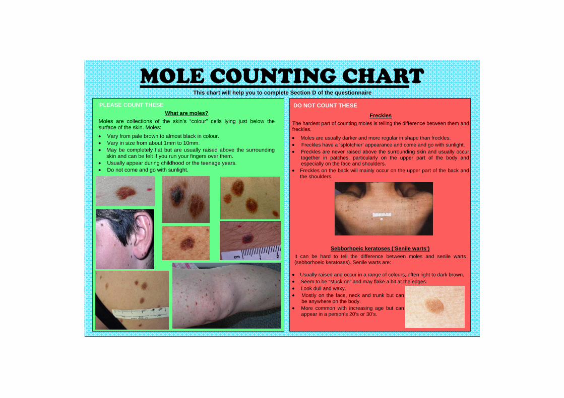
MOLE COUNTING CHART This chart will help you to complete Section D of the questionnaire
What are moles? Moles are collections of the skin’s “colour” cells lying just below the surface of the skin. Moles: • Vary from pale brown to almost black in colour. • Vary in size from about 1mm to 10mm. • May be completely flat but are usually raised above the surrounding
skin and can be felt if you run your fingers over them. • Usually appear during childhood or the teenage years. • Do not come and go with sunlight.
Freckles The hardest part of counting moles is telling the difference between them and freckles.
• Moles are usually darker and more regular in shape than freckles. • Freckles have a ‘splotchier’ appearance and come and go with sunlight. • Freckles are never raised above the surrounding skin and usually occur
together in patches, particularly on the upper part of the body and especially on the face and shoulders.
• Freckles on the back will mainly occur on the upper part of the back and the shoulders.
• Usually raised and occur in a range of colours, often light to dark brown. • Seem to be “stuck on” and may flake a bit at the edges. • Look dull and waxy. • Mostly on the face, neck and trunk but can
be anywhere on the body. • More common with increasing age but can
appear in a person’s 20’s or 30’s.
Sebborhoeic keratoses (‘Senile warts’) It can be hard to tell the difference between moles and senile warts (sebborhoeic keratoses). Senile warts are:
PLEASE COUNT THESE DO NOT COUNT THESE

287APPENDIX G
Questionnaire

IdId
EntryEntry
EntryEntry
EntryEntry
IDID Start TimeStart TimeDateDate
Good morning/afternoon, could I please speak to
Please enter your ID, today's date and the participant's sex.
Participant's AgeParticipant's Age SexSex
MHS No.MHS No.
EntryEntry
My name is ......... and I am calling about the telephone interview for the Western Australian Melanoma Health Study. Would now be a convenient time to do the interview and do you have your brochure with you?
If:- asked who is calling/why you are calling- someone else answers- the participant is not there- you get an answering machinePlease refer to your questionnaire guide for standard responses.
Once speaking to the participant:
If YES - continue to next page (they MUST have the brochure to continue)If NO - refer to questionnaire guide

Have you had a chance to complete the height and weight questions and do your mole count ?
If NO, arrange time to call back today, or another day [refer to interviewing roster], for these answers.
Now go to page 3a.
If YES, ask questions below and continue to page 3a.
cm
What is your weight in kilograms? kg
We would also like to know the number of moles on your back. Please refer to the diagram in question D2.
How many moles do you have in section A, or from the base of your neck to the top of your armpits ?
D2
How many moles do you have in section B, or from the top of your armpit to the top of your underpants ?
moles
What is your height in centimetres?A2
A3
moles
Before we start, I’d like to ask you to get a pen and paper, as I’ll ask you to note down a few things a bit later on in the interview to help you with your answers. [Wait whilst items obtained].

SECTION B : COLOURING AND SKIN TYPE
SECTION A : PERSONAL DETAILS
Single De facto Married Divorced WidowedSingle De facto Married Divorced Widowed
Red (including auburn)
Fair or blonde (including white)
Light or mouse brown
Grey
Dark brown
Black
Red (including auburn)
Fair or blonde (including white)
Light or mouse brown
Grey
Dark brown
Black
Blue
Grey
Green
Hazel
Brown
Black
Blue
Grey
Green
Hazel
Brown
Black
Very fair
Fair
Olive or brown
Dark
Very fair
Fair
Olive or brown
Dark
Which colour best describes your skin before tanning or on areas never exposed to the sun, such as the inside of your upper arm?
Could you confirm your date of birth is :
B3
Which colour best describes the colour of your eyes?B2
Which colour best describes your natural hair colour at age 18?
B1
Page 3Version 4
What is your marital status?

B4 Which statement best describes what would happen to your skin if it were exposed to bright sunlight for the first time in summer, for one hour in the middle of the day, without any protection (e.g. sunscreen, clothing)?
Get a severe sunburn with blistering
Have a painful sunburn for a few days followed by peeling
Get mildly burnt followed by some tanning
Go brown without any sunburn
Get a severe sunburn with blistering
Have a painful sunburn for a few days followed by peeling
Get mildly burnt followed by some tanning
Go brown without any sunburn
B5 Which of the following best describes what would happen to your skin if it were repeatedly exposed to bright sunlight in summer without any protection (e.g. sunscreen, clothing)?
Which statement best describes what would happen to your skin if it were exposed to bright sunlight for the first time in summer, for one hour in the middle of the day, without any protection (e.g. sunscreen, clothing)?
B6
Always burns, never tans
Usually burns, never tans
Sometimes burns, usually tans
Never burns, always tans
Always burns, never tans
Usually burns, never tans
Sometimes burns, usually tans
Never burns, always tans
Go very brown and deeply tanned
Get moderately tanned
Get mildly or occasionally tanned
Get no suntan at all or only get freckled
Go very brown and deeply tanned
Get moderately tanned
Get mildly or occasionally tanned
Get no suntan at all or only get freckled

Please look at the faces above questions B7 and B8 in your brochure. Each of the faces shows some degree of freckling, from none to very many. For the following questions, we are looking for your best estimate.
B7
None Very few Few Some Many Very ManyNone Very few Few Some Many Very Many
Which of these faces best describes how many freckles you had at the end of summer as an adult; that is, when you were over 18 ?
B8
None Very few Few Some Many Very manyNone Very few Few Some Many Very many
Page 5
Which of these faces best describes how many freckles you had at the end of summer during childhood; that is, up until you were 17 years old?

How old were you when you first started smoking cigarettes or tobacco at least once a day?
Have you ever smoked cigarettes or tobacco once a day for six months or more?
C1
No
Yes
No
Yes
SECTION C : LIFESTYLE HISTORY
C2
years old
C3 Do you smoke cigarettes or tobacco at least once a day now?
No
Yes
No
Yes
C4 How old were you when you stopped smoking cigarettes or tobacco at least once a day?
years old
C5 Over your life time, how many total years have you smoked?
years
C6 On average, over the entire time that you smoked, how much did you smoke each day?
cigarettes per day (manufactured cigarettes only, not self rolled cigarettes)
of loose tobacco per day
cigars per day50g = 1 pouch of tobacco 1g = 1 self rolled cigarette
grams
ounces
grams
ounces (includes loose tobacco smoked in pipes or self rolled cigarettes)
Page 6

SECTION D : MOLES
The following question is about the number of moles that you have. Again, we are looking for your best estimate.
Please look at the diagrams in question D1. They show various numbers of moles. Which picture best describes how many moles you have now ?
D1
None Few Some ManyNone Few Some Many
Page 7

F2
In which country were you born ?
I would now like to ask you some questions about your background and family history.
DO NOT READ OPTIONS TO PARTICIPANT, CODE FROM RESPONSE
If other selected, please type country's name in the box.
What year did you first arrive in Australia?What year did you first arrive in Australia?
Where did you live for the majority of the time from when you were born to when you were 12 years of age ?
Country Country
State/County/Province/RegionState/County/Province/Region
Where did you live for the majority of the time between the ages of 13 and 19 ?
Where did you live for the majority of the time from the age of 20 to now ?
CountryCountry
State/County/Province/Region State/County/Province/Region
CountryCountry
State/County/Province/Region State/County/Province/Region
F1
F3
F4
F5
What is the highest level of education you have completed?
F6
City/TownCity/Town
City/TownCity/Town
City/TownCity/Town

I'd now like to ask you some questions about your ethnic background and the ethnic background of your family.
How would you describe your ethnic background ?
Indigenous Australian (Aboriginal, Torres Strait Islander)Indigenous Australian (Aboriginal, Torres Strait Islander)
South East Asian (Brunei, Cambodia, Indonesia, Laos, Malaysia, Myanmar/Burma, Philippines,
Singapore, Thailand, Vietnam)
South East Asian (Brunei, Cambodia, Indonesia, Laos, Malaysia, Myanmar/Burma, Philippines,
Singapore, Thailand, Vietnam)
North-East Asian (China, Hong Kong, Japan, Korea, Macau, Taiwan)North-East Asian (China, Hong Kong, Japan, Korea, Macau, Taiwan)
South-Asian (Afghanistan, Bangladesh, India, Nepal, Pakistan, Sri Lanka)South-Asian (Afghanistan, Bangladesh, India, Nepal, Pakistan, Sri Lanka)
Middle Eastern (Israel, Iran, Iraq, Lebanon, Turkey, Egypt)Middle Eastern (Israel, Iran, Iraq, Lebanon, Turkey, Egypt)
Pacific Islander (New Zealand Maori or originated from Pacific Islands, Hawaii, New Guinea)Pacific Islander (New Zealand Maori or originated from Pacific Islands, Hawaii, New Guinea)
African (Originating from North Africa, Sub-Saharan Africa, Zimbabwe, Indigenous South African)African (Originating from North Africa, Sub-Saharan Africa, Zimbabwe, Indigenous South African)
F7A
DO NOT READ OPTIONS TO PARTICIPANT, CODE FROM RESPONSEIf participant wishes to select two answers, they may, however do not suggest this option.
Caucasian - English (Orginated from England)Caucasian - English (Orginated from England)
Caucasian - Scottish, Irish or Welsh (Orginated from Scotland, Ireland or Wales)Caucasian - Scottish, Irish or Welsh (Orginated from Scotland, Ireland or Wales)
Caucasian - Other Northern European (Austria, Latvia, Lithuania, Estonia, Denmark, France, Germany, Luxembourg, Netherlands/Holland, Sweden, Norway, Finland, Switzerland, other Western/Northern European countries)
Caucasian - Other Northern European (Austria, Latvia, Lithuania, Estonia, Denmark, France, Germany, Luxembourg, Netherlands/Holland, Sweden, Norway, Finland, Switzerland, other Western/Northern European countries)
Caucasian - Southern European (Greece, Italy, Portugal, Spain, Former Yugoslavia, Malta, Cyprus, other Southern European countries)Caucasian - Southern European (Greece, Italy, Portugal, Spain, Former Yugoslavia, Malta, Cyprus, other Southern European countries)
Caucasian - Eastern European (Bulgaria, Former Czechoslovakia, Hungary, Poland, Romania, Former USSR, other Eastern European countries)Caucasian - Eastern European (Bulgaria, Former Czechoslovakia, Hungary, Poland, Romania, Former USSR, other Eastern European countries)
Caucasian - Other CaucasianCaucasian - Other Caucasian Please specify - Please specify -

B How would you describe the ethnic background of your biological mother?
Indigenous Australian (Aboriginal, Torres Strait Islander)Indigenous Australian (Aboriginal, Torres Strait Islander)
South East Asian (Brunei, Cambodia, Indonesia, Laos, Malaysia, Myanmar/Burma, Philippines,
Singapore, Thailand, Vietnam)
South East Asian (Brunei, Cambodia, Indonesia, Laos, Malaysia, Myanmar/Burma, Philippines,
Singapore, Thailand, Vietnam)
North-East Asian (China, Hong Kong, Japan, Korea, Macau, Taiwan)North-East Asian (China, Hong Kong, Japan, Korea, Macau, Taiwan)
South-Asian (Afghanistan, Bangladesh, India, Nepal, Pakistan, Sri Lanka)South-Asian (Afghanistan, Bangladesh, India, Nepal, Pakistan, Sri Lanka)
Middle Eastern (Israel, Iran, Iraq, Lebanon, Turkey, Egypt)Middle Eastern (Israel, Iran, Iraq, Lebanon, Turkey, Egypt)
Pacific Islander (New Zealand Maori or originated from Pacific Islands, Hawaii, New Guinea)Pacific Islander (New Zealand Maori or originated from Pacific Islands, Hawaii, New Guinea)
African (Originating from North Africa, Sub-Saharan Africa, Zimbabwe, Indigenous South African)African (Originating from North Africa, Sub-Saharan Africa, Zimbabwe, Indigenous South African)
Caucasian - English (Orginated from England)Caucasian - English (Orginated from England)
Caucasian - Scottish, Irish or Welsh (Orginated from Scotland, Ireland or Wales)Caucasian - Scottish, Irish or Welsh (Orginated from Scotland, Ireland or Wales)
Caucasian - Other Northern European (Austria, Latvia, Lithuania, Estonia, Denmark, France, Germany, Luxembourg, Netherlands/Holland, Sweden, Norway, Finland, Switzerland, other Western/Northern European countries)
Caucasian - Other Northern European (Austria, Latvia, Lithuania, Estonia, Denmark, France, Germany, Luxembourg, Netherlands/Holland, Sweden, Norway, Finland, Switzerland, other Western/Northern European countries)
Caucasian - Southern European (Greece, Italy, Portugal, Spain, Former Yugoslavia, Malta, Cyprus, other Southern European countries)Caucasian - Southern European (Greece, Italy, Portugal, Spain, Former Yugoslavia, Malta, Cyprus, other Southern European countries)
Caucasian - Eastern European (Bulgaria, Former Czechoslovakia, Hungary, Poland, Romania, Former USSR, other Eastern European countries)Caucasian - Eastern European (Bulgaria, Former Czechoslovakia, Hungary, Poland, Romania, Former USSR, other Eastern European countries)
Caucasian - Other CaucasianCaucasian - Other Caucasian Please specify - Please specify -

How would you describe the ethnic background of your biological father?
Indigenous Australian (Aboriginal, Torres Strait Islander)Indigenous Australian (Aboriginal, Torres Strait Islander)
South East Asian (Brunei, Cambodia, Indonesia, Laos, Malaysia, Myanmar/Burma, Philippines,
Singapore, Thailand, Vietnam)
South East Asian (Brunei, Cambodia, Indonesia, Laos, Malaysia, Myanmar/Burma, Philippines,
Singapore, Thailand, Vietnam)
North-East Asian (China, Hong Kong, Japan, Korea, Macau, Taiwan)North-East Asian (China, Hong Kong, Japan, Korea, Macau, Taiwan)
South-Asian (Afghanistan, Bangladesh, India, Nepal, Pakistan, Sri Lanka)South-Asian (Afghanistan, Bangladesh, India, Nepal, Pakistan, Sri Lanka)
Middle Eastern (Israel, Iran, Iraq, Lebanon, Turkey, Egypt)Middle Eastern (Israel, Iran, Iraq, Lebanon, Turkey, Egypt)
Pacific Islander (New Zealand Maori or originated from Pacific Islands, Hawaii, New Guinea)Pacific Islander (New Zealand Maori or originated from Pacific Islands, Hawaii, New Guinea)
African (Originating from North Africa, Sub-Saharan Africa, Zimbabwe, Indigenous South African)African (Originating from North Africa, Sub-Saharan Africa, Zimbabwe, Indigenous South African)
C
Caucasian - English (Orginated from England)Caucasian - English (Orginated from England)
Caucasian - Scottish, Irish or Welsh (Orginated from Scotland, Ireland or Wales)Caucasian - Scottish, Irish or Welsh (Orginated from Scotland, Ireland or Wales)
Caucasian - Other Northern European (Austria, Latvia, Lithuania, Estonia, Denmark, France, Germany, Luxembourg, Netherlands/Holland, Sweden, Norway, Finland, Switzerland, other Western/Northern European countries)
Caucasian - Other Northern European (Austria, Latvia, Lithuania, Estonia, Denmark, France, Germany, Luxembourg, Netherlands/Holland, Sweden, Norway, Finland, Switzerland, other Western/Northern European countries)
Caucasian - Southern European (Greece, Italy, Portugal, Spain, Former Yugoslavia, Malta, Cyprus, other Southern European countries)Caucasian - Southern European (Greece, Italy, Portugal, Spain, Former Yugoslavia, Malta, Cyprus, other Southern European countries)
Caucasian - Eastern European (Bulgaria, Former Czechoslovakia, Hungary, Poland, Romania, Former USSR, other Eastern European countries)Caucasian - Eastern European (Bulgaria, Former Czechoslovakia, Hungary, Poland, Romania, Former USSR, other Eastern European countries)
Caucasian - Other CaucasianCaucasian - Other Caucasian Please specify - Please specify -

D How would you describe the ethnic background of your mother's mother?
Indigenous Australian (Aboriginal, Torres Strait Islander)Indigenous Australian (Aboriginal, Torres Strait Islander)
South East Asian (Brunei, Cambodia, Indonesia, Laos, Malaysia, Myanmar/Burma, Philippines,
Singapore, Thailand, Vietnam)
South East Asian (Brunei, Cambodia, Indonesia, Laos, Malaysia, Myanmar/Burma, Philippines,
Singapore, Thailand, Vietnam)
North-East Asian (China, Hong Kong, Japan, Korea, Macau, Taiwan)North-East Asian (China, Hong Kong, Japan, Korea, Macau, Taiwan)
South-Asian (Afghanistan, Bangladesh, India, Nepal, Pakistan, Sri Lanka)South-Asian (Afghanistan, Bangladesh, India, Nepal, Pakistan, Sri Lanka)
Middle Eastern (Israel, Iran, Iraq, Lebanon, Turkey, Egypt)Middle Eastern (Israel, Iran, Iraq, Lebanon, Turkey, Egypt)
Pacific Islander (New Zealand Maori or originated from Pacific Islands, Hawaii, New Guinea)Pacific Islander (New Zealand Maori or originated from Pacific Islands, Hawaii, New Guinea)
African (Originating from North Africa, Sub-Saharan Africa, Zimbabwe, Indigenous South African)African (Originating from North Africa, Sub-Saharan Africa, Zimbabwe, Indigenous South African)
Caucasian - English (Orginated from England)Caucasian - English (Orginated from England)
Caucasian - Scottish, Irish or Welsh (Orginated from Scotland, Ireland or Wales)Caucasian - Scottish, Irish or Welsh (Orginated from Scotland, Ireland or Wales)
Caucasian - Other Northern European (Austria, Latvia, Lithuania, Estonia, Denmark, France, Germany, Luxembourg, Netherlands/Holland, Sweden, Norway, Finland, Switzerland, other Western/Northern European countries)
Caucasian - Other Northern European (Austria, Latvia, Lithuania, Estonia, Denmark, France, Germany, Luxembourg, Netherlands/Holland, Sweden, Norway, Finland, Switzerland, other Western/Northern European countries)
Caucasian - Southern European (Greece, Italy, Portugal, Spain, Former Yugoslavia, Malta, Cyprus, other Southern European countries)Caucasian - Southern European (Greece, Italy, Portugal, Spain, Former Yugoslavia, Malta, Cyprus, other Southern European countries)
Caucasian - Eastern European (Bulgaria, Former Czechoslovakia, Hungary, Poland, Romania, Former USSR, other Eastern European countries)Caucasian - Eastern European (Bulgaria, Former Czechoslovakia, Hungary, Poland, Romania, Former USSR, other Eastern European countries)
Caucasian - Other CaucasianCaucasian - Other Caucasian Please specify - Please specify -

How would you describe the ethnic background of your mother's father?
Indigenous Australian (Aboriginal, Torres Strait Islander)Indigenous Australian (Aboriginal, Torres Strait Islander)
South East Asian (Brunei, Cambodia, Indonesia, Laos, Malaysia, Myanmar/Burma, Philippines,
Singapore, Thailand, Vietnam)
South East Asian (Brunei, Cambodia, Indonesia, Laos, Malaysia, Myanmar/Burma, Philippines,
Singapore, Thailand, Vietnam)
North-East Asian (China, Hong Kong, Japan, Korea, Macau, Taiwan)North-East Asian (China, Hong Kong, Japan, Korea, Macau, Taiwan)
South-Asian (Afghanistan, Bangladesh, India, Nepal, Pakistan, Sri Lanka)South-Asian (Afghanistan, Bangladesh, India, Nepal, Pakistan, Sri Lanka)
Middle Eastern (Israel, Iran, Iraq, Lebanon, Turkey, Egypt)Middle Eastern (Israel, Iran, Iraq, Lebanon, Turkey, Egypt)
Pacific Islander (New Zealand Maori or originated from Pacific Islands, Hawaii, New Guinea)Pacific Islander (New Zealand Maori or originated from Pacific Islands, Hawaii, New Guinea)
African (Originating from North Africa, Sub-Saharan Africa, Zimbabwe, Indigenous South African)African (Originating from North Africa, Sub-Saharan Africa, Zimbabwe, Indigenous South African)
E
Caucasian - English (Orginated from England)Caucasian - English (Orginated from England)
Caucasian - Scottish, Irish or Welsh (Orginated from Scotland, Ireland or Wales)Caucasian - Scottish, Irish or Welsh (Orginated from Scotland, Ireland or Wales)
Caucasian - Other Northern European (Austria, Latvia, Lithuania, Estonia, Denmark, France, Germany, Luxembourg, Netherlands/Holland, Sweden, Norway, Finland, Switzerland, other Western/Northern European countries)
Caucasian - Other Northern European (Austria, Latvia, Lithuania, Estonia, Denmark, France, Germany, Luxembourg, Netherlands/Holland, Sweden, Norway, Finland, Switzerland, other Western/Northern European countries)
Caucasian - Southern European (Greece, Italy, Portugal, Spain, Former Yugoslavia, Malta, Cyprus, other Southern European countries)Caucasian - Southern European (Greece, Italy, Portugal, Spain, Former Yugoslavia, Malta, Cyprus, other Southern European countries)
Caucasian - Eastern European (Bulgaria, Former Czechoslovakia, Hungary, Poland, Romania, Former USSR, other Eastern European countries)Caucasian - Eastern European (Bulgaria, Former Czechoslovakia, Hungary, Poland, Romania, Former USSR, other Eastern European countries)
Caucasian - Other CaucasianCaucasian - Other Caucasian Please specify - Please specify -

F How would you describe the ethnic background of your father's mother?
Indigenous Australian (Aboriginal, Torres Strait Islander)Indigenous Australian (Aboriginal, Torres Strait Islander)
South East Asian (Brunei, Cambodia, Indonesia, Laos, Malaysia, Myanmar/Burma, Philippines,
Singapore, Thailand, Vietnam)
South East Asian (Brunei, Cambodia, Indonesia, Laos, Malaysia, Myanmar/Burma, Philippines,
Singapore, Thailand, Vietnam)
North-East Asian (China, Hong Kong, Japan, Korea, Macau, Taiwan)North-East Asian (China, Hong Kong, Japan, Korea, Macau, Taiwan)
South-Asian (Afghanistan, Bangladesh, India, Nepal, Pakistan, Sri Lanka)South-Asian (Afghanistan, Bangladesh, India, Nepal, Pakistan, Sri Lanka)
Middle Eastern (Israel, Iran, Iraq, Lebanon, Turkey, Egypt)Middle Eastern (Israel, Iran, Iraq, Lebanon, Turkey, Egypt)
Pacific Islander (New Zealand Maori or originated from Pacific Islands, Hawaii, New Guinea)Pacific Islander (New Zealand Maori or originated from Pacific Islands, Hawaii, New Guinea)
African (Originating from North Africa, Sub-Saharan Africa, Zimbabwe, Indigenous South African)African (Originating from North Africa, Sub-Saharan Africa, Zimbabwe, Indigenous South African)
Caucasian - English (Orginated from England)Caucasian - English (Orginated from England)
Caucasian - Scottish, Irish or Welsh (Orginated from Scotland, Ireland or Wales)Caucasian - Scottish, Irish or Welsh (Orginated from Scotland, Ireland or Wales)
Caucasian - Other Northern European (Austria, Latvia, Lithuania, Estonia, Denmark, France, Germany, Luxembourg, Netherlands/Holland, Sweden, Norway, Finland, Switzerland, other Western/Northern European countries)
Caucasian - Other Northern European (Austria, Latvia, Lithuania, Estonia, Denmark, France, Germany, Luxembourg, Netherlands/Holland, Sweden, Norway, Finland, Switzerland, other Western/Northern European countries)
Caucasian - Southern European (Greece, Italy, Portugal, Spain, Former Yugoslavia, Malta, Cyprus, other Southern European countries)Caucasian - Southern European (Greece, Italy, Portugal, Spain, Former Yugoslavia, Malta, Cyprus, other Southern European countries)
Caucasian - Eastern European (Bulgaria, Former Czechoslovakia, Hungary, Poland, Romania, Former USSR, other Eastern European countries)Caucasian - Eastern European (Bulgaria, Former Czechoslovakia, Hungary, Poland, Romania, Former USSR, other Eastern European countries)
Caucasian - Other CaucasianCaucasian - Other Caucasian Please specify - Please specify -

G How would you describe the ethnic background of your father's father?
Indigenous Australian (Aboriginal, Torres Strait Islander)Indigenous Australian (Aboriginal, Torres Strait Islander)
South East Asian (Brunei, Cambodia, Indonesia, Laos, Malaysia, Myanmar/Burma, Philippines,
Singapore, Thailand, Vietnam)
South East Asian (Brunei, Cambodia, Indonesia, Laos, Malaysia, Myanmar/Burma, Philippines,
Singapore, Thailand, Vietnam)
North-East Asian (China, Hong Kong, Japan, Korea, Macau, Taiwan)North-East Asian (China, Hong Kong, Japan, Korea, Macau, Taiwan)
South-Asian (Afghanistan, Bangladesh, India, Nepal, Pakistan, Sri Lanka)South-Asian (Afghanistan, Bangladesh, India, Nepal, Pakistan, Sri Lanka)
Middle Eastern (Israel, Iran, Iraq, Lebanon, Turkey, Egypt)Middle Eastern (Israel, Iran, Iraq, Lebanon, Turkey, Egypt)
Pacific Islander (New Zealand Maori or originated from Pacific Islands, Hawaii, New Guinea)Pacific Islander (New Zealand Maori or originated from Pacific Islands, Hawaii, New Guinea)
African (Originating from North Africa, Sub-Saharan Africa, Zimbabwe, Indigenous South African)African (Originating from North Africa, Sub-Saharan Africa, Zimbabwe, Indigenous South African)
Caucasian - English (Orginated from England)Caucasian - English (Orginated from England)
Caucasian - Scottish, Irish or Welsh (Orginated from Scotland, Ireland or Wales)Caucasian - Scottish, Irish or Welsh (Orginated from Scotland, Ireland or Wales)
Caucasian - Other Northern European (Austria, Latvia, Lithuania, Estonia, Denmark, France, Germany, Luxembourg, Netherlands/Holland, Sweden, Norway, Finland, Switzerland, other Western/Northern European countries)
Caucasian - Other Northern European (Austria, Latvia, Lithuania, Estonia, Denmark, France, Germany, Luxembourg, Netherlands/Holland, Sweden, Norway, Finland, Switzerland, other Western/Northern European countries)
Caucasian - Southern European (Greece, Italy, Portugal, Spain, Former Yugoslavia, Malta, Cyprus, other Southern European countries)Caucasian - Southern European (Greece, Italy, Portugal, Spain, Former Yugoslavia, Malta, Cyprus, other Southern European countries)
Caucasian - Eastern European (Bulgaria, Former Czechoslovakia, Hungary, Poland, Romania, Former USSR, other Eastern European countries)Caucasian - Eastern European (Bulgaria, Former Czechoslovakia, Hungary, Poland, Romania, Former USSR, other Eastern European countries)
Caucasian - Other CaucasianCaucasian - Other Caucasian Please specify - Please specify -

I’d now like to ask you some questions about your family history.
F8
Yes
No
Don't know
Has your biological mother ever been told by a doctor that she has any type of skin cancer?Has your biological mother ever been told by a doctor that she has any type of skin cancer?
No
Don't know
F9A
Yes
No
Don't know
Did she have a melanoma?Did she have a melanoma?
No
Don't know
F9B
Yes
No
Don't know
Did she have another type of skin cancer that wasn’t a melanoma?Did she have another type of skin cancer that wasn’t a melanoma?
No
Don't know
F10
Yes - Please specify
No
Don't know
Has your biological mother ever been told by a doctor that she has any other type of cancer?Has your biological mother ever been told by a doctor that she has any other type of cancer?
No
Don't know BreastBreast
BladderBladder
ColorectalColorectal
KidneyKidney
StomachStomach
PancreasPancreas
OvarianOvarian
LeukemiaLeukemia
ThyroidThyroid
LungLung
LymphomaLymphoma
UterusUterus
Other - Please SpecifyOther - Please Specify
F11
Yes
No
Don't know
Has your biological father ever been told by a doctor that he has any type of skin cancer ?Has your biological father ever been told by a doctor that he has any type of skin cancer ?
No
Don't know
F12A
F12B
Yes
No
Don't know
Did he have a malignant melanoma?Did he have a malignant melanoma?
No
Don't know
Yes
No
Don't know
Did he have another type of skin cancer that wasn’t a melanoma?Did he have another type of skin cancer that wasn’t a melanoma?
No
Don't know
Yes - Please specify
No
Don't know
Has your biological father ever been told by a doctor that he has any other type of cancer?Has your biological father ever been told by a doctor that he has any other type of cancer?
No
Don't know
F13
BladderBladder
ColorectalColorectal
KidneyKidney
LeukemiaLeukemia
LungLung
LymphomaLymphoma
Other - Please SpecifyOther - Please Specify
ThyroidThyroid
StomachStomach
PancreasPancreas
ProstateProstate

F14
Yes
No
Don't know
Do you have any full brothers? That is, brothers with the same mother and father as you.Do you have any full brothers? That is, brothers with the same mother and father as you.
No
Don't know
How many full brothers do you have? How many full brothers do you have?
Yes
No
Don't know
Have any of your full brothers ever been told by a doctor that they had any type of skin cancer?Have any of your full brothers ever been told by a doctor that they had any type of skin cancer?
No
Don't know
How many brothers were told this? How many brothers were told this?
Yes
No
Don't know
Did any of them have a malignant melanoma?Did any of them have a malignant melanoma?
No
Don't know
Yes
No
Don't know
Did any of them have another type of skin cancer that wasn’t a melanoma?Did any of them have another type of skin cancer that wasn’t a melanoma?
No
Don't know
How many brothers were told this?How many brothers were told this?
How many brothers were told this?How many brothers were told this?
Yes - Please Specify How Many
No
Don't know
Have any of your full brothers ever told by a doctor that they had any other type of cancer?Have any of your full brothers ever told by a doctor that they had any other type of cancer?
No
Don't know
BladderBladder
ColorectalColorectal
KidneyKidney
LungLung
LymphomaLymphoma
PancreasPancreas
F21F21
F15F15
F16F16
F17F17
F18AF18A
F19F19
F18BF18B
F20F20
LeukemiaLeukemia ProstateProstate
StomachStomach
ThyroidThyroid
OtherOther

F23
Yes
No
Don't know
Do you have any half brothers? That is, brothers with the same mother OR father as you.Do you have any half brothers? That is, brothers with the same mother OR father as you.
No
Don't know
How many half brothers do you have? How many half brothers do you have?
Yes
No
Don't know
Have any of your half brothers ever been told by a doctor that they have any type of skin cancer?Have any of your half brothers ever been told by a doctor that they have any type of skin cancer?
No
Don't know
How many brothers were told this? How many brothers were told this?
Yes
No
Don't know
Did any of them have a malignant melanoma?Did any of them have a malignant melanoma?
No
Don't know
Yes
No
Don't know
Did any of them have another type of skin cancer that wasn’t a melanoma?Did any of them have another type of skin cancer that wasn’t a melanoma?
No
Don't know
How many brothers were told this?How many brothers were told this?
How many brothers were told this?How many brothers were told this?
Yes - Please Specify How Many
No
Don't know
Were any of your half brothers ever told by a doctor that they had any other type of cancer?Were any of your half brothers ever told by a doctor that they had any other type of cancer?
No
Don't know
F24F24
F25F25
F26F26
F27AF27A
F28F28
F27BF27B
F29F29
F30F30
BladderBladder
ColorectalColorectal
KidneyKidney
LeukemiaLeukemia ProstateProstate
PancreasPancreas
LymphomaLymphoma
LungLung StomachStomach
ThyroidThyroid
OtherOther
F32
Yes
No
Don't know
Do you have any full sisters? That is, sisters with the same mother and father as you.Do you have any full sisters? That is, sisters with the same mother and father as you.
No
Don't know
How many full sisters do you have? How many full sisters do you have?
Yes
No
Don't know
Have any of your full sisters ever been told by a doctor that they have any type of skin cancer?Have any of your full sisters ever been told by a doctor that they have any type of skin cancer?
No
Don't know
How many sisters were told this? How many sisters were told this?
Yes
No
Don't know
Did any of them have a malignant melanoma?Did any of them have a malignant melanoma?
No
Don't know
Yes
No
Don't know
Did any of them have another type of skin cancer that wasn’t a melanoma?Did any of them have another type of skin cancer that wasn’t a melanoma?
No
Don't know
How many sisters were told this?How many sisters were told this?
How many sisters were told this?How many sisters were told this?
Yes - Please Specify How Many
No
Don't know
Were any of your full sisters ever told by a doctor that they had any other type of cancer?Were any of your full sisters ever told by a doctor that they had any other type of cancer?
No
Don't know
F33F33
F34F34
F35F35
F36AF36A
F37F37
F36BF36B
F38F38
F39F39
OtherOther
ThyroidThyroidLungLung
LymphomaLymphoma
PancreasPancreas
StomachStomach
BladderBladder
ColorectalColorectal
KidneyKidney
LeukemiaLeukemia
BreastBreast
OvarianOvarian
UterusUterus

F41
Yes
No
Don't know
Do you have any half sisters? That is, sisters with the same mother or father as you.Do you have any half sisters? That is, sisters with the same mother or father as you.
No
Don't know
How many half sisters do you have? How many half sisters do you have?
Yes
No
Don't know
Have any of your half sisters ever been told by a doctor that they had any type of skin cancer?Have any of your half sisters ever been told by a doctor that they had any type of skin cancer?
No
Don't know
How many sisters were told this? How many sisters were told this?
Yes
No
Don't know
Did any of them have a malignant melanoma?Did any of them have a malignant melanoma?
No
Don't know
Yes
No
Don't know
Did any of them have another type of skin cancer that wasn’t a melanoma?Did any of them have another type of skin cancer that wasn’t a melanoma?
No
Don't know
How many sisters were told this?How many sisters were told this?
How many sisters were told this?How many sisters were told this?
Yes - Please Specify How Many
No
Don't know
Were any of your half sisters ever been told by a doctor that they had any other type of cancer?Were any of your half sisters ever been told by a doctor that they had any other type of cancer?
No
Don't know
F42F42
F43F43
F44F44
F45AF45A
F46F46
F45BF45B
F47F47
F48F48
OtherOther
LymphomaLymphoma
PancreasPancreas
StomachStomach
OvarianOvarian
UterusUterus
ThyroidThyroidLungLungBladderBladder
ColorectalColorectal
KidneyKidney
LeukemiaLeukemia
BreastBreast

F50 Are you a twin, triplet or other multiple birth?
Yes, a twin
Yes, a triplet
Yes, other multiple birth
No
Don't know
Are you a twin, triplet or other multiple birth?Are you a twin, triplet or other multiple birth?
Yes, a triplet
Yes, other multiple birth
No
Don't know

F51
Yes
No
Don't know
Do you have any biological children? Do you have any biological children?
No
Don't know
How many children do you have? How many children do you have?
Yes
No
Don't know
Have any of your children ever been told by a doctor that they have any type of skin cancer?Have any of your children ever been told by a doctor that they have any type of skin cancer?
No
Don't know
F52F52
F53F53
How many children have been told this? How many children have been told this?
This only refers to biological children, not step-children.
F54F54
Yes
No
Don't know
Did any of them have a malignant melanoma?Did any of them have a malignant melanoma?
No
Don't know
F55AF55A
How many children were told this?How many children were told this?
Yes
No
Don't know
Did any of them have another type of skin cancer that wasn’t a melanoma?Did any of them have another type of skin cancer that wasn’t a melanoma?
No
Don't know
F56F56
F55BF55B
How many children were told this?How many children were told this?F57F57
Yes
No
Don't know
Were any of your children ever told by a doctor that they had any other type of cancer?Were any of your children ever told by a doctor that they had any other type of cancer?
No
Don't know
F58F58
BreastBreast
OtherOtherPancreasPancreas
OvarianOvarianColorectalColorectal
KidneyKidney
LymphomaLymphoma
BladderBladder LungLung
LeukemiaLeukemia ProstateProstate
StomachStomach
UterusUterus
ThyroidThyroid

I am now going to ask you some questions about time that you've spent outdoors at various ages. By 'outdoors', I mean the time you spent outdoors and not under any shade between 9am and 5pm.
Please remember we are looking for your best estimate.
To help you with the next set of questions, it might be useful to write down ‘not under any shade’ and ‘between 9am and 5pm’, to act as a reminder when answering the questions.”
I'd like to start by asking you about time outdoors in the warmer months, that is, spring and summer, when you were 5-12 years of age or in primary school.
How many hours per day did you usually spend outdoors and not under any shade, between 9am and 5pm in the warmer months on:
School days School days
WeekendsWeekends
ORDon't knowDon't know
ORDon't knowDon't know
G1.3
Mainly indoorsSplit between indoors and outdoorsMainly outdoors
On average, in the warmer months, during the hours that you were at school, were your activities:On average, in the warmer months, during the hours that you were at school, were your activities:
Split between indoors and outdoorsMainly outdoors
G1.4
Mainly indoorsSplit between indoors and outdoorsMainly outdoors
On average, were these activities:On average, were these activities:
Split between indoors and outdoorsMainly outdoors
I'd now like you to think about recreational activities that you did during the warmer months (for example, playing sport, going to the beach, playing musical instruments) between 9am and 5pm.
G1.1,1.2
hrs
hrs
I'd now like to ask you about time outdoors in the cooler months, that is, autumn and winter, when you were 5-12 years of age.
How many hours per day did you usually spend outdoors and not under any shade, between 9am and 5pm in the cooler months on:
School days School days
WeekendsWeekends
ORDon't knowDon't know
ORDon't knowDon't know
G1.7
Mainly indoorsSplit between indoors and outdoorsMainly outdoors
On average, in the cooler months, during the hours that you were at school, were your activities:On average, in the cooler months, during the hours that you were at school, were your activities:
Split between indoors and outdoorsMainly outdoors
G1.8
Mainly indoorsSplit between indoors and outdoorsMainly outdoors
On average, were these activities:On average, were these activities:
Split between indoors and outdoorsMainly outdoors
I'd now like you to think about recreational activities that you did during the cooler months (for example, playing sport, going to the beach, playing musical instruments) between 9am and 5pm.
G1.5,1.6
hrs
hrs

I'd now like to ask you some questions about when you were 13-19 years of age.
How many hours per day did you usually spend outdoors and not under any shade, between 9am and 5pm in the warmer months on:
School or week days School or week days
WeekendsWeekends
ORDon't knowDon't know
ORDon't knowDon't know
G2.4
Mainly indoorsSplit between indoors and outdoorsMainly outdoors
On average, in the warmer months, during the hours that you were at school or working, were your activities:On average, in the warmer months, during the hours that you were at school or working, were your activities:
Split between indoors and outdoorsMainly outdoors
G2.5
Mainly indoorsSplit between indoors and outdoorsMainly outdoors
On average, were these activities:On average, were these activities:
Split between indoors and outdoorsMainly outdoors
I'd now like you to think about recreational activities that you did during the warmer months (for example, playing sport, going to the beach, playing musical instruments) between 9am and 5pm.
G2.1
During these years, what was your main occupation?
I'd now like to ask you about time outdoors in the warmer months, that is, spring and summer, when you were 13-19 years of age.
I'd now like you to think about all the jobs that you had during these years (including studying).
G2.2,2.3
hrs
hrs
OtherOther

How many hours per day did you usually spend outdoors and not under any shade, between 9am and 5pm in the cooler months on:
School or week days School or week days
WeekendsWeekends
ORDon't knowDon't know
ORDon't knowDon't know
G2.8
Mainly indoorsSplit between indoors and outdoorsMainly outdoors
On average, in the cooler months, during the hours that you were at school or working, were your activities:On average, in the cooler months, during the hours that you were at school or working, were your activities:
Split between indoors and outdoorsMainly outdoors
G2.9
I'd now like you to think about recreational activities that you did during the cooler months (for example, playing sport, going to the beach, playing musical instruments) between 9am and 5pm.
I'd now like to ask you about time outdoors in the cooler months, that is, autumn and winter, when you were 13-19 years of age.
I'd now like you to think about all the jobs that you had during these years (including studying).
Mainly indoorsSplit between indoors and outdoorsMainly outdoors
On average, were these activities:On average, were these activities:
Split between indoors and outdoorsMainly outdoors
G2.6,2.7
hrs
hrs

I'd now like to ask you some questions about when you were 20-39 years of age.
G3.2
Mainly indoorsSplit between indoors and outdoorsMainly outdoors
On average, during the hours that you were working between 9am and 5pm, were your activities:On average, during the hours that you were working between 9am and 5pm, were your activities:
Split between indoors and outdoorsMainly outdoors
G3.3
Mainly indoorsSplit between indoors and outdoorsMainly outdoors
In the warmer months, on average, were these activities:In the warmer months, on average, were these activities:
Split between indoors and outdoorsMainly outdoors
I'd now like you to think about recreational activities that you did (for example, playing sport, going to the beach, playing musical instruments) between 9am and 5pm.
G3.1
During these years, what was your main occupation?
I'd now like you to think about all the jobs that you had during these years (including studying).
G3.4
Mainly indoorsSplit between indoors and outdoorsMainly outdoors
In the cooler months, on average, were these activities:In the cooler months, on average, were these activities:
Split between indoors and outdoorsMainly outdoors
OtherOther

I'd now like to ask you some questions about when you were 40-65 years of age.
G4.3
Mainly indoorsSplit between indoors and outdoorsMainly outdoors
On average, during the hours that you were working between 9am and 5pm, were your activities:On average, during the hours that you were working between 9am and 5pm, were your activities:
Split between indoors and outdoorsMainly outdoors
G4.4
Mainly indoorsSplit between indoors and outdoorsMainly outdoors
In the warmer months, on average, were these activities:In the warmer months, on average, were these activities:
Split between indoors and outdoorsMainly outdoors
I'd now like you to think about recreational activities that you did (for example, playing sport, going to the beach, playing musical instruments) between 9am and 5pm.
G4.1
During these years, what was your main occupation?
I'd now like you to think about all the jobs that you had during these years (including studying).
G4.5
Mainly indoorsSplit between indoors and outdoorsMainly outdoors
In the cooler months, on average, were these activities:In the cooler months, on average, were these activities:
Split between indoors and outdoorsMainly outdoors
Year Retired ?Year Retired ?
OtherOther

I'd now like to ask you some questions about when you were 65 years of age till now.
G5.3
Mainly indoorsSplit between indoors and outdoorsMainly outdoors
On average, during the hours that you were working between 9am and 5pm, were your activities:On average, during the hours that you were working between 9am and 5pm, were your activities:
Split between indoors and outdoorsMainly outdoors
G5.4
Mainly indoorsSplit between indoors and outdoorsMainly outdoors
In the warmer months, on average, were these activities:In the warmer months, on average, were these activities:
Split between indoors and outdoorsMainly outdoors
I'd now like you to think about recreational activities that you did (for example, playing sport, going to the beach, playing musical instruments) between 9am and 5pm.
G5.1
During these years, what was your main occupation?
I'd now like you to think about all the jobs that you had during these years (including studying).
G5.5
Mainly indoorsSplit between indoors and outdoorsMainly outdoors
In the cooler months, on average, were these activities:In the cooler months, on average, were these activities:
Split between indoors and outdoorsMainly outdoors
Year Retired ?Year Retired ?
OtherOther

I'd now like to ask you some questions about sunburn for various ages. Before we start, can I ask you to write down the following options, which might help you with your responses: "0, 1-5, 6-10, more than 10".
G6.1
0Between 1 and 5 timesBetween 6 and 10 timesMore than 10 timesDon't know
How many times were you sunburnt so as to cause pain for 2 or more days when you were between 5-12 years of age?
How many times were you sunburnt so as to cause pain for 2 or more days when you were between 5-12 years of age?
Between 1 and 5 timesBetween 6 and 10 timesMore than 10 timesDon't know
0Between 1 and 5 timesBetween 6 and 10 timesMore than 10 timesDon't know
How many times were you sunburnt so severely as to cause blisters between 5-12 years of age?How many times were you sunburnt so severely as to cause blisters between 5-12 years of age?
Between 1 and 5 timesBetween 6 and 10 timesMore than 10 timesDon't know
G6.2

G7.1
0Between 1 and 5 timesBetween 6 and 10 timesMore than 10 timesDon't know
How many times were you sunburnt so as to cause pain for 2 or more days when you were between 13-19 years of age?
How many times were you sunburnt so as to cause pain for 2 or more days when you were between 13-19 years of age?
Between 1 and 5 timesBetween 6 and 10 timesMore than 10 timesDon't know
0Between 1 and 5 timesBetween 6 and 10 timesMore than 10 timesDon't know
How many times were you sunburnt so severely as to cause blisters between 13-19 years of age?How many times were you sunburnt so severely as to cause blisters between 13-19 years of age?
Between 1 and 5 timesBetween 6 and 10 timesMore than 10 timesDon't know
G7.2
0Between 1 and 5 timesBetween 6 and 10 timesMore than 10 timesDon't know
How many times were you sunburnt so severely as to cause blisters since you were 20 years of age? How many times were you sunburnt so severely as to cause blisters since you were 20 years of age?
Between 1 and 5 timesBetween 6 and 10 timesMore than 10 timesDon't know
0Between 1 and 5 timesBetween 6 and 10 timesMore than 10 timesDon't know
How many times were you sunburnt so as to cause pain for 2 or more days since you were 20 years of age?How many times were you sunburnt so as to cause pain for 2 or more days since you were 20 years of age?
Between 1 and 5 timesBetween 6 and 10 timesMore than 10 timesDon't know
G8.1G8.1
G8.2G8.2

I'd now like to ask you about sunbed use.
G9
YesNoDon't know
Have you ever used a sunlamp or sunbed for any reason on more than one occasion?Have you ever used a sunlamp or sunbed for any reason on more than one occasion?
NoDon't know
How old were you when you first used one?How old were you when you first used one?
How old were you when you last used one?How old were you when you last used one?
About how many sunlamp or sunbed sessions have you had in total, over your lifetime?
About how many sunlamp or sunbed sessions have you had in total, over your lifetime?
G13 In what types of locations have you used a sunlamp or sunbed?
Tanning salonTanning salon
Hairdressers, beauty salonsHairdressers, beauty salons
Gymnasium, health club/spa or fitness club/spaGymnasium, health club/spa or fitness club/spa
Hospital or medical facilityHospital or medical facility
Private homePrivate home
Other - Please specifyOther - Please specify
Don't knowDon't know
DO NOT READ OPTIONS TO PARTICIPANT.
The participant may select more than one answer.
G10G10
G11G11
G12G12

I'd now like to ask you some questions about your medical history.
How many melanomas have you been told you've had by a doctor?How many melanomas have you been told you've had by a doctor?
H1.1
How many non-melanoma skin cancers have you been told you've had by a doctor? How many non-melanoma skin cancers have you been told you've had by a doctor?
H1.2a
H1.3
How many skin cancers are you unsure about?How many skin cancers are you unsure about?
Yes
No
Have you had any skin cancers and are unsure what they were?Have you had any skin cancers and are unsure what they were? No
H1.4H1.4
Yes
No
Don't know
Have you had any non-melanoma skin cancers, that is basal cell carcinomas or squamous cell carcinomas? These are often called BCC's or SCC's.
Have you had any non-melanoma skin cancers, that is basal cell carcinomas or squamous cell carcinomas? These are often called BCC's or SCC's.
No
Don't know
H1.2b

When did a doctor tell you that you had a melanoma for the X time?
Where on your body was your X melanoma situated?
Where were you living when you were told by a doctor about your X melanoma?
How large is the scar where your X melanoma was removed?
Please fill in the table for each melanoma.
You should then ask the questions above the table, replacing X with first, second, third, etc.
Number of melanomasNumber of melanomas
YearYear
Don't knowDon't know
MonthMonth
1st
AnatomicalAnatomical
SideSide
StateState
Please specify countryPlease specify country
Size of scarSize of scar
MonthMonth
2nd
Don't knowDon't know
SideSide
AnatomicalAnatomical StateState
Please specify countryPlease specify country
Size of scarSize of scar
MonthMonth
3rd
Don't knowDon't know
SideSide
AnatomicalAnatomical StateState
Please specify countryPlease specify country
Size of scarSize of scar
YearYear
YearYear

When did a doctor tell you that you had a melanoma for the X time?
Where on your body was your X melanoma situated?
YearYear
MonthMonth AnatomicalAnatomical
SideSide
Don't knowDon't know
MonthMonth AnatomicalAnatomical
Where were you living when you were told by a doctor about your X melanoma?
StateState
Please specify countryPlease specify country
5th
Don't knowDon't know
SideSide
StateState
Please specify countryPlease specify country
MonthMonth AnatomicalAnatomical
6th SideSide
StateState
How large is the scar where your X melanoma was removed?
Size of scarSize of scar
Please specify countryPlease specify country
Size of scarSize of scar
Don't knowDon't know
Size of scarSize of scar
YearYear
YearYear
MonthMonth
YearYear
Don't knowDon't know
AnatomicalAnatomical
SideSide
StateState
Please specify countryPlease specify country
Size of scarSize of scar
MonthMonth
YearYear
Don't knowDon't know
AnatomicalAnatomical
SideSide
StateState
Please specify countryPlease specify country
Size of scarSize of scar
4th
7th
8th

When did a doctor tell you that you had a melanoma for the X time?
Where on your body was your X melanoma situated?
YearYear
MonthMonth AnatomicalAnatomical
SideSide
Don't knowDon't know
MonthMonth AnatomicalAnatomical
Where were you living when you were told by a doctor about your X melanoma?
StateState
Please specify countryPlease specify country
10th
Don't knowDon't know
SideSide
StateState
Please specify countryPlease specify country
MonthMonth AnatomicalAnatomical
11th SideSide
StateState
How large is the scar where your X melanoma was removed?
Size of scarSize of scar
Please specify countryPlease specify country
Size of scarSize of scar
Don't knowDon't know
Size of scarSize of scar
YearYear
YearYear
MonthMonth
YearYear
Don't knowDon't know
AnatomicalAnatomical
SideSide
StateState
Please specify countryPlease specify country
Size of scarSize of scar
MonthMonth
YearYear
Don't knowDon't know
AnatomicalAnatomical
SideSide
StateState
Please specify countryPlease specify country
Size of scarSize of scar
9th
12th
13th

How many have you been told you've had?How many have you been told you've had?H16H16
H17H17 What year were you first told you had an SCC?What year were you first told you had an SCC?
H15H15Yes
No
Don't know
Of the non-melanoma skin cancers that you've been told about, were any of them squamous cell carcinomas or SCC?
Of the non-melanoma skin cancers that you've been told about, were any of them squamous cell carcinomas or SCC?
No
Don't know
Yes
No
Don't know
Of the non-melanoma skin cancers that you've been told about, were any of them basal cell carcinomas or BCC?
Of the non-melanoma skin cancers that you've been told about, were any of them basal cell carcinomas or BCC?
No
Don't know
H12H12
How many have you been told you've had?How many have you been told you've had?H13H13
H14H14 What year were you first told you had a BCC?What year were you first told you had a BCC?
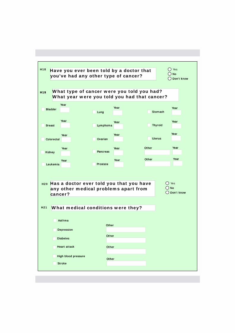
H18 Yes
No
Don't know
Have you ever been told by a doctor that you've had any other type of cancer?Have you ever been told by a doctor that you've had any other type of cancer? No
Don't know
H19H19
H20 Yes
No
Don't know
Has a doctor ever told you that you have any other medical problems apart from cancer?
Has a doctor ever told you that you have any other medical problems apart from cancer?
No
Don't know
BreastBreast
BladderBladder
ColorectalColorectal
KidneyKidney
LungLung
LymphomaLymphoma
Ovarian Ovarian
PancreasPancreas
ThyroidThyroid
UterusUterus
LeukemiaLeukemia ProstateProstate
StomachStomach
What type of cancer were you told you had?What year were you told you had that cancer?
OtherOther
OtherOther
YearYear
YearYear
YearYear
YearYear
YearYear
YearYear
YearYear
YearYear
YearYear
YearYear
YearYear
YearYear
YearYear
YearYear
YearYear
AsthmaAsthma
H21 What medical conditions were they?
DiabetesDiabetes
Heart attackHeart attack
High blood pressureHigh blood pressure
StrokeStroke
DepressionDepression
OtherOther
OtherOther
OtherOther
OtherOther

I1 Do you have any comments, or other information that you think would be useful?Do you have any comments, or other information that you think would be useful?
I2 For the interviewer: do you have any comments regarding this interview?For the interviewer: do you have any comments regarding this interview?
End TimeEnd Time
Please check with participant whether or not they have done their blood sample yet, if they consented to give one.
If YES - please thank themIf NO - please let them know it would be greatly appreciated if they could do it ASAP.
Please see QxQ for details on types of blood forms.

328 Appendix G. Questionnaire
329APPENDIX H
Questionnaire Brochure

330
App
endixH
.Q
uestionnaireB
rochure
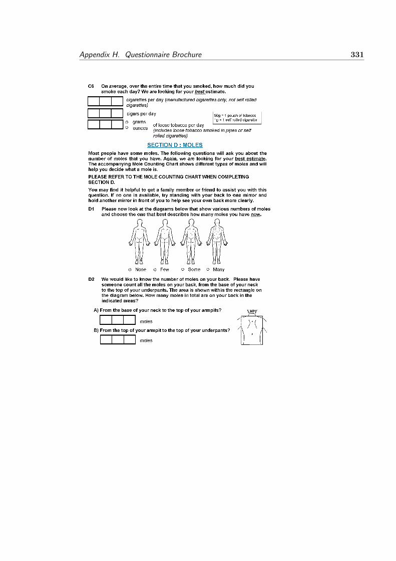
Appendix H. Questionnaire Brochure 331

332 Appendix H. Questionnaire Brochure

333APPENDIX I
MRsnphap R Package User Manual

Package ‘MRsnphap’
May 18, 2010
Type Package
Title A modeling framework for Mendelian Randomisation studies of single SNPsand haplotypes
Version 1.0.0
Date 2010-05-05
Depends MASS, stats, SimHap
Author Gemma Cadby
Maintainer Gemma Cadby <[email protected]>
Description MRsnphap is a package for modelling Mendelian Randomisation studies. Itcan perform single SNP and haplotype association analyses for continuousNormal outcomes measured in population-based samples. MRsnphap usesthe estimation maximisation techniques for inferring haplotypic phase, andincorporates a multiple-imputation approach to deal with the uncertainty ofimputed haplotypes in Mendelian Randomisation analyses.
License GPL2
R topics documented:
mrhap.quant . . . . . . . . . . . . . . . . . . . . . . . . . . . . . . . . . . . . . . . . . 1mrsnp.quant . . . . . . . . . . . . . . . . . . . . . . . . . . . . . . . . . . . . . . . . . 3
mrhap.quant Mendelian Randomisation using Haplotypes as Instruments
Description
mrhap.quant is used for Mendelian Randomisation modelling of epidemiological data withcontinuous outcomes, where one or more haplotypes are used as instruments for somemodifiable exposure.
Usage
mrhap.quant(outcome, exposure, covariates = NULL, geneticmodel, pheno,
haplo, sim, effect="add",small = NULL)
1

Arguments
outcome a continuous outcome.
exposure a modifiable exposure
covariates a list of covariates in the form"x1+...+xn". Defaults to NULL.
geneticmodel the haplotype/s used as the instrument. May be coded as either additive,recessive or dominant.
haplo a haplotype object made by make.haplo.rare.
pheno a dataframe containing phenotype data.
sim the number of simulations from which to evaluate the results.
effect the haplotypic effect type: "add" for additive, "dom" for dominant and"rec" for recessive. Defaults to additive.
small a small sample correction. Defaults to NULL.
Details
If an instrument is considered weak, a warning file with the current date will be stored inthe working directory. Use getwd() to locate this directory.
Value
mrhap.quant returns an object of class MRhap.
The summary function can be used to obtain and print a summary of the results.
An object of class MRhap is a list containing the following components:
instruments formula containing instruments and covariates
structual structural formula containing the outcome regressed on exposure and co-variates
results a table containing the coefficients, standard errors, p-values and 95% con-fidence limits of the parameter estimates, averaged over the sim modelsperformed
empiricalResults
a list containing the coefficients, standard errors and p-values calculatedat each simulation.
observations number of observations
weakfstat mean F-Statistic for the first stage regression of exposure on instrument/s,averaged over the sim models performed
sarganp mean P-values for the Sargan test statistic, averaged over the sim mod-els performed. The sarganp will only be shown when there are moreinstruments than exposures
DWHp mean P-values for the Durbin-Wu-Haussman statistic, averaged over thesim models performed
effect the haplotypic effect modelled, ‘ADDITIVE’, ‘DOMINANT’ or ‘RECES-SIVE’.
2

Author(s)
Gemma Cadby
References
Carter, K.W., McCaskie, P.A., Palmer, L.J. (2008). SimHap GUI: An intuitive graphicaluser interface for genetic association analysis. BMC Bioinformatics 2008 Dec 25;9(1):557.
McCaskie, P.A., Carter, K.W, Hazelton, M., Palmer, L.J. (2007) SimHap: A comprehen-sive modeling framework for epidemiological outcomes and a simulation-based approach tohaplotypic analysis of population-based data, [online] www.genepi.org.au/simhap.
Baum, C.F., Schaffer, M.E., Stillman, S. (2007) Enhanced routines for instrumental vari-ables/GMM Estimation and testing, Stata Journal, 7 (4), 465-506.
See Also
mrsnp.quant
Examples
data(SNP.dat)
# convert SNP.dat to format required by infer.haplos
haplo.dat <- SNP2Haplo(SNP.dat)
data(pheno.dat)
# generate haplotype frequencies and haplotype design matrix
myinfer<-infer.haplos(haplo.dat)
# print haplotype frequencies generated by infer.haplos
myinfer$hap.freq
# generate haplo object where haplotypes with a frequency
# below min.freq are grouped as a category called "rare"
myhaplo<-make.haplo.rare(myinfer,min.freq=0.05)
mymodel.hap<- mrhap.quant(outcome="BT", exposure="VitD", covariates="AGE", geneticmodel="h.N1AA",
pheno=pheno.dat, haplo=myhaplo, sim=10, effect="add")
summary(mymodel.hap)
mrsnp.quant Mendelian Randomisation using Single SNPs as Instruments
Description
mrsnp.quant is used for Mendelian Randomisation modelling of epidemiological data withcontinuous outcomes, where one or more SNPs are used as instruments for some modifiableexposure.
3

Usage
mrsnp.quant(outcome, exposure, covariates = NULL, geneticmodel,
geno, pheno, small = NULL)
Arguments
outcome a continuous outcome.
exposure a modifiable exposure
covariates a list of covariates in the form"x1+...+xn". Defaults to NULL.
geneticmodel the SNP used as the instrument. May be coded as either additive, reces-sive or dominant.
geno a dataframe containing genotype data.
pheno a dataframe containing phenotype data.
small a small sample correction. Defaults to NULL.
Details
If an instrument is considered weak, a warning message will be printed.
Value
mrsnp.quant returns an object of class MRsnp.
The summary function can be used to obtain and print a summary of the results.
An object of class MRsnp is a list containing the following components:
instruments formula containing instruments and covariates
structual structural formula containing the outcome regressed on exposure and co-variates
results a table containing the coefficients, standard errors, p-values and 95% con-fidence limits of the parameter estimates
observations number of observations
weakfstat F-Statistic for the first stage regression of exposure on instrument/s
sarganstat Sargan test statistic for the overidentification test of all instruments. Thesarganstat will only be shown when there are more instruments thanexposures
sarganp P-value for the Sargan test statistic. The sarganp will only be shownwhen there are more instruments than exposures
DWHstat Durbin-Wu-Haussman statistic for the test of endogeneity.
DWHp P-value for the Durbin-Wu-Haussman statistic
residualerror Residual error of the model
Author(s)
Gemma Cadby
4

References
Carter, K.W., McCaskie, P.A., Palmer, L.J. (2008). SimHap GUI: An intuitive graphicaluser interface for genetic association analysis. BMC Bioinformatics 2008 Dec 25;9(1):557
McCaskie, P.A., Carter, K.W, Hazelton, M., Palmer, L.J. (2007) SimHap: A comprehen-sive modeling framework for epidemiological outcomes and a simulation-based approach tohaplotypic analysis of population-based data, [online] www.genepi.org.au/simhap.
Baum, C.F., Schaffer, M.E., Stillman, S. (2007) Enhanced routines for instrumental vari-ables/GMM Estimation and testing, Stata Journal, 7 (4), 465-506.
See Also
mrhap.quant
Examples
data(SNP.dat)
#convert SNP.dat to format required by mrsnp.quant
geno.dat<- SNP2Geno(SNP.dat, baseline=c("MM", "11", "GG", "CC"))
data(pheno.dat)
mymodel.snp<- mrsnp.quant(outcome="BT", exposure="VitD", covariates="AGE", geneticmodel="SNP_1_add",
geno=geno.dat, pheno=pheno.dat)
summary(mymodel.snp)
5
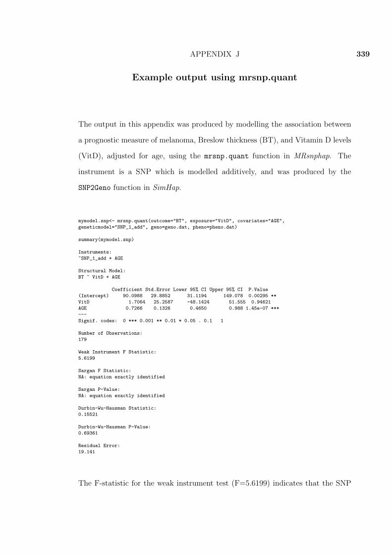
339APPENDIX J
Example output using mrsnp.quant
The output in this appendix was produced by modelling the association between
a prognostic measure of melanoma, Breslow thickness (BT), and Vitamin D levels
(VitD), adjusted for age, using the mrsnp.quant function in MRsnphap. The
instrument is a SNP which is modelled additively, and was produced by the
SNP2Geno function in SimHap.
mymodel.snp<- mrsnp.quant(outcome="BT", exposure="VitD", covariates="AGE",
geneticmodel="SNP_1_add", geno=geno.dat, pheno=pheno.dat)
summary(mymodel.snp)
Instruments:
~SNP_1_add + AGE
Structural Model:
BT ~ VitD + AGE
Coefficient Std.Error Lower 95% CI Upper 95% CI P.Value
(Intercept) 90.0988 29.8852 31.1194 149.078 0.00295 **
VitD 1.7064 25.2587 -48.1424 51.555 0.94621
AGE 0.7266 0.1326 0.4650 0.988 1.45e-07 ***
---
Signif. codes: 0 *** 0.001 ** 0.01 * 0.05 . 0.1 1
Number of Observations:
179
Weak Instrument F Statistic:
5.6199
Sargan F Statistic:
NA: equation exactly identified
Sargan P-Value:
NA: equation exactly identified
Durbin-Wu-Hausman Statistic:
0.15521
Durbin-Wu-Hausman P-Value:
0.69361
Residual Error:
19.141
The F-statistic for the weak instrument test (F=5.6199) indicates that the SNP

340 Appendix J. Example output using mrsnp.quant
is a weak instrument for Vitamin D and should not be used. The Durbin-Wu
Hausman p-value of 0.69361 indicates that Vitamin D should not be treated as
an endogeneous regressor.

341APPENDIX K
Example output using mrhap.quant
The output in this appendix was produced by modelling the association between
a prognostic measure of melanoma, Breslow thickness (BT), and Vitamin D levels
(VitD), adjusted for age, using the mrhap.quant function in MRsnphap. The in-
strument is a haplotype, h.N1AA, which is modelled additively, and was produced
by the haplo.dat and infer.haplos functions in SimHap.
The Mendelian randomisation model is run 100 times, and the average of the co-
efficients, statistics and p-values are reported.
mymodel.hap<- mrhap.quant(outcome="BT", exposure="VitD", covariates="AGE",
geneticmodel="h.N1AA", pheno=pheno.dat, haplo=myhaplo, sim=100, effect="add")
[1] "* Finding highest individual frequency ..."
[1] " Done"
[1] "* Populating individual haplotypes and posterior probabilities ..."
[1] " Done"
[1] "* Distributing individual occurrences across the simulations by posterior probability ..."
[1] " 25%"
[1] " 50%"
[1] " 75%"
[1] " 90%"
[1] " Done"
[1] "* Generating a random pattern of individuals for each simulation ..."
[1] " Done"
[1] "* Constructing datafiles and performing model for each simulation ..."
[1] " Done"
summary(mymodel.hap)
Instruments:
~h.N1AA + AGE
Structural Model:
BT ~ VitD + AGE
Coefficients:
Coefficient Std.error Lower 95% CI Upper 95% CI P.Value
(Intercept) 204.0052 580.5689 -941.7227 1349.733 0.1655
VitD -97.0130 502.4302 -1088.5376 894.511 0.4170
AGE 0.9529 1.1717 -1.3594 3.265 0.0815 .
---
Signif. codes: 0 *** 0.001 ** 0.01 * 0.05 . 0.1 1
Number of Observations:
180
Weak Instrument F Statistic:

342 Appendix K. Example output using mrhap.quant
[1] 1.4697
Sargan P-Value:
[1] NA
Durbin-Wu-Hausman P-Value:
[1] 0.25544
The F-statistic for the weak instrument test (F=1.4697) indicates that the h.N1AA
haplotype is a weak instrument for Vitamin D levels and should not be used. The
Durbin-Wu Hausman p-value of 0.25544 indicates that Vitamin D should not be
treated as an endogeneous regressor.