Geert Bekaert, Marie Hoerova and Marco Lo Duca

Risk, Uncertainty and Monetary Policy

DP 05/2011-102

Electronic copy available at: http://ssrn.com/abstract=1561171

* We thank Tobias Adrian, Gianni Amisano, David DeJong, Bartosz Mackowiak, Frank Smets, José Valentim, Jonathan Wright and seminar participants at the European Central Bank, the FRB Philadelphia, the Midwest Macroeconomics Meetings (East Lansing), the Annual Seminar on Banking, Financial Stability and Risk (Sao Paulo), the Vienna Macroeconomics Workshop (Rome), the Financial Management Association Meetings (New York) and the Annual IMF Jacques Polak Research Conference (Washington) for helpful comments and suggestions. Falk Bräuning and Francesca Fabbri provided excellent research assistance. The views expressed do not necessarily reflect those of the European Central Bank or the Eurosystem.

Risk, Uncertainty and Monetary Policy*

Geert Bekaert

Columbia GSB

Marie Hoerova

ECB

Marco Lo Duca

ECB

May 2011

Abstract

We document a strong co-movement between the VIX, the stock market option-based implied volatility, and monetary policy. We decompose the VIX into two components, a proxy for risk aversion and expected stock market volatility (“uncertainty”), and analyze their dynamic interactions with monetary policy in a structural vector autoregressive framework. A lax monetary policy decreases risk aversion after about five months. Monetary authorities react to periods of high uncertainty by easing monetary policy. These results are robust to controlling for business cycle movements. We further investigate channels through which monetary policy may affect risk aversion, e.g., through its effects on broad liquidity measures and credit.

JEL Classification: E44; E 52; G12; G20; E32

Keywords: Monetary policy; Option implied volatility; Risk aversion; Uncertainty;

Business cycle; Stock market volatility dynamics

Electronic copy available at: http://ssrn.com/abstract=1561171

I. Introduction

A popular indicator of risk aversion in financial markets, the VIX index, shows strong co-

movements with measures of the monetary policy stance. Figure 1 considers the cross-

correlogram between the real interest rate (the Fed funds rate minus inflation), a measure

of the monetary policy stance, and the logarithm of end-of-month readings of the VIX

index. The VIX index essentially measures the “risk-neutral” expected stock market

variance for the US S&P500 index. The correlogram reveals a very strong positive

correlation between real interest rates and future VIX levels. While the current VIX is

positively associated with future real rates, the relationship turns negative and significant

after 13 months: high VIX readings are correlated with expansionary monetary policy in

the medium-run future.

The strong interaction between a “fear index” (Whaley (2000)) in the asset markets

and monetary policy indicators may have important implications for a number of

literatures. First, the recent crisis has rekindled the idea that lax monetary policy can be

conducive to financial instability. The Federal Reserve’s pattern of providing liquidity to

financial markets following market tensions, which became known as the “Greenspan

put,” has been cited as one of the contributing factors to the build up of a speculative

bubble prior to the 2007-09 financial crisis.1 Whereas some rather informal stories have

linked monetary policy to risk-taking in financial markets (Rajan (2006), Adrian and Shin

(2008), Borio and Zhu (2008)), it is fair to say that no extant research establishes a firm

empirical link between monetary policy and risk aversion in asset markets.2

Second, Bloom (2009) and Bloom, Floetotto and Jaimovich (2009) show that

heightened “economic uncertainty” decreases employment and output. It is therefore

conceivable that the monetary authority responds to uncertainty shocks, in order to affect

economic outcomes. However, the VIX index, used by Bloom (2009) to measure

uncertainty, can be decomposed into a component that reflects actual expected stock

market volatility (uncertainty) and a residual, the so-called variance premium (see, for 1 Investors increasingly believed that when market conditions were to deteriorate, the Fed would step in and inject liquidity until the outlook improved. The perception may have become embedded in asset pricing in the form of higher valuations, narrower credit spreads, and excessive risk-taking. See, for example, “Greenspan Put may be Encouraging Complacency,” Financial Times, December 8, 2000. 2 For recent empirical evidence that monetary policy affects the riskiness of loans granted by banks see, for example, Altunbas, Gambacorta and Marquéz-Ibañez (2010), Ioannidou, Ongena and Peydró (2009), Jiménez, Ongena, Peydró and Saurina (2009), and Maddaloni and Peydró (2010).

1

example, Carr and Wu (2009)), that reflects risk aversion and other non-linear pricing

effects, perhaps even Knightian uncertainty. Establishing which component drives the

strong comovements between the monetary policy stance and the VIX is therefore

particularly important.

Third, analyzing the relationship between monetary policy and the VIX and its

components may help clarify the relationship between monetary policy and the stock

market, explored in a large number of empirical papers (Thorbecke (1997), Rigobon and

Sack (2004), Bernanke and Kuttner (2005)). The extant studies all find that expansionary

(contractionary) monetary policy affects the stock market positively (negatively).

Interestingly, Bernanke and Kuttner (2005) ascribe the bulk of the effect to easier

monetary policy lowering risk premiums, reflecting both a reduction in economic and

financial volatility and an increase in the capacity of financial investors to bear risk. By

using the VIX and its two components, we test the effect of monetary policy on stock

market risk, but also provide more precise information on the exact channel.

This article characterizes the dynamic links between risk aversion, economic

uncertainty and monetary policy in a simple vector-autoregressive (VAR) system. Such

analysis faces a number of difficulties. First, because risk aversion and the stance of

monetary policy are jointly endogenous variables and display strong contemporaneous

correlation (see Figure 1), a structural interpretation of the dynamic effects requires

identifying restrictions. Monetary policy may indeed affect asset prices through its effect

on risk aversion, as suggested by the literature on monetary policy news and the stock

market, but monetary policy makers may also react to a nervous and uncertain market

place by loosening monetary policy. In fact, Rigobon and Sack (2003) find that the

Federal Reserve does systematically respond to stock prices.3

Second, the relationship between risk aversion and monetary policy may also reflect

the joint response to an omitted variable, with business cycle variation being a prime

candidate. Recessions may be associated with high risk aversion (see Campbell and

Cochrane (1999) for a model generating counter-cyclical risk aversion) and at the same

3 The two papers by Rigobon and Sack (2003, 2004) use an identification scheme based on the heteroskedasticity of stock market returns. Given that we view economic uncertainty as an important endogenous variable in its own right with links to the real economy and risk premiums, we cannot use such an identification scheme.

2

time lead to lax monetary policy. Our VARs always include a business cycle indicator.

Third, measuring the monetary policy stance is the subject of a large literature (see, for

example, Bernanke and Mihov (1998a)); and measuring policy shocks correctly is

difficult. Models featuring time-varying risk aversion and/or uncertainty, such as Bekaert,

Engstrom and Xing (2009), imply an equilibrium contemporaneous link between interest

rates and risk aversion and uncertainty, through precautionary savings effects for

example. Such relation should not be associated with a policy shock. However, our

results are robust to alternative measures of the monetary policy stance and shocks.

The remainder of the paper is organized as follows. In Section II, we use a simple

analytical framework and a series of numerical examples to provide intuition on how the

VIX is related to the actual expected variance of stock returns and to risk preferences.

While the literature has proposed a number of risk appetite measures (see Baker and

Wurgler (2007) and Coudert and Gex (2008)), we show that our measure is

monotonically increasing in risk aversion in a variety of economic settings. This

motivates our empirical strategy in which we split the VIX into a pure volatility

component (“uncertainty”) and a residual, which should be more closely associated with

risk aversion. In Section III, we analyze the dynamic effects of monetary policy on risk

aversion and uncertainty and vice versa, under various identification schemes. In Section

IV, we conduct a long series of robustness tests. Our results are remarkably robust to

alternative methods to identify monetary policy shocks and the structural VAR

parameters more generally. In the final section, we empirically examine various channels

through which monetary policy may affect risk aversion and private sector risk-taking

behavior, as suggested by recent research. Specifically, we consider the effects through

the balance sheet of financial intermediaries (as proxied by repo growth and the growth

rates of broad money aggregates) and through the expansion of credit (using the growth

of credit and credit-to-GDP ratio).

Our main findings are as follows. A lax monetary policy decreases risk aversion in

the stock market after about five months. This effect is persistent, lasting for two years.

Moreover, monetary policy shocks account for a significant proportion of the variance of

risk aversion. On the other hand, periods of high uncertainty are followed by a looser

monetary policy stance. The effect of monetary policy on risk aversion is independent

3

and does not necessarily run through repo or credit growth. Finally, it is the risk aversion

component of the VIX that has the strongest effect on the business cycle, not the

uncertainty component.

II. Interpreting the VIX

The VIX represents the option-implied expected volatility on the S&P500 index with a

horizon of 30 calendar days (22 trading days). This volatility concept is often referred to

as “implied volatility.” The computation of the VIX index relies on theoretical results

showing that option prices can be used to replicate any bounded payoff pattern; in fact,

they can be used to replicate Arrow-Debreu securities (Breeden and Litzenberger (1978),

Bakshi and Madan (2000)). Britten-Jones and Neuberger (2000) and Bakshi, Kapadia and

Madan (2003) show how to infer “risk-neutral” or “risk-adjusted” expected volatility for

a stock index from option prices. The VIX index measures implied volatility using a

weighted average of European-style S&P500 call and put option prices that straddle a 30-

day maturity and cover a wide range of strikes (see CBOE (2004) for more details).

Importantly, this estimate is model-free and does not rely on an option pricing model.

Measuring Risk Aversion and Uncertainty

While the VIX obviously reflects stock market uncertainty, its link to option prices

means it also harbours information about risk and risk aversion. Indeed, financial markets

often view the VIX as a measure of risk aversion and fear in the market place. Because

there are well-accepted techniques to measure the physical expected variance, we can

split the VIX into a measure of stock market or economic uncertainty, and a residual that

should be more closely associated with risk aversion. In the context of an external habit

model, Bekaert, Engstrom and Xing (2009) show how “risk aversion” and “economic

uncertainty” may have different effects on asset prices. These differences may be

important to acknowledge in monetary policy transmission.

The difference between the squared VIX and an estimate of the conditional variance

is typically called the variance premium (see, e.g., Carr and Wu (2009)).4 The variance

premium is nearly always positive and displays substantial time-variation. Recent finance

4 In the technical finance literature, the variance premium is actually the negative of the variable that we use. By switching the sign, our indicator increases with risk aversion, whereas the variance premium becomes more negative with risk aversion.

4

models attribute these facts either to non-Gaussian components in fundamentals and

(stochastic) risk aversion (see, for instance, Bekaert and Engstrom (2009), Bollerslev,

Tauchen and Zhou (2009), Drechsler and Yaron (2009)) or Knightian uncertainty (see

Drechsler (2009)).

In the empirical analysis, we use end-of-month VIX levels. To decompose the VIX

index into its two components, we borrow a measure of the conditional variance of stock

returns from Bekaert and Engstrom (2009). They project monthly realized variances

(computed using squared 5-minute returns) on the past realized variance, the past

(squared) VIX, the dividend yield and a real short interest rate. The fitted value of this

regression, which is primarily driven by the past realized variance and the VIX, is the

estimated physical expected variance. We call the logarithm of this estimate

“uncertainty” (uct). We call the logarithm of the difference between the squared VIX and

this conditional variance, “risk aversion” (rat). We plot the two series in Figure 2.5

The VIX and Risk

To obtain intuition how the VIX is related to the actual (“physical”) expected

variance of stock returns and to risk preferences, we analyze a one-period discrete state

economy. Imagine a stock return distribution with three different states , as follows: ix

Good state: axg with probability 2/)1( p ,

Bad state : axb with probability 2/)1( p ,

Crash state: with probability cxc p ,

where 0 , and are parameters to be determined. We set them to match

statistics in the data for the US stock market - the mean, the variance (standard deviation)

and the skewness - while fixing the crash return at an empirically plausible number.

0a 0c

The mean is given by:

pcppcxp

xp

X bg

)1(2

1

2

1. (1)

The variance is given by:

5 The estimated uncertainty series is less “jaggedy” than it would be if only the past realized variance would be used to compute it (as in Bollerslev, Tauchen and Zhou, 2009), which in turn helps smooth the risk aversion process.

5

2222 )()(2

1)(

2

1XcpXa

pXa

pV

(2)

and the skewness ( ) by: Sk

3332

3

)()(2

1)(

2

1XcpXa

pXa

pSkV

. (3)

Consider a one-period world such that the investor has a power utility function over

wealth and in equilibrium she invests her entire wealth in the stock market:

1

)~

()

~(

10 RW

EWU , (4)

where R~

is the gross return on the stock market, is initial wealth and 0W is the

coefficient of relative risk aversion.

The “pricing kernel” in this economy is given by marginal utility, denoted by , and

is proportional to . Hence, the stochastic part of the pricing kernel moves inversely

with the return on the stock market. When the stock market is down, marginal utility is

relatively high and vice versa.

m

R~

The physical variance of the stock market is exogenous in this economy, and is

simply given by V . This variance is computed using the actual probabilities. The VIX

represents the “risk-neutral” conditional variance. It is computed using the so-called

“risk-neutral probabilities,” which are simply probabilities adjusted for risk.

In particular, for a general state probability i for state , the risk-neutral probability

is:

i

mE

R

mE

m ii

ii

RNi

. (5)

So, for a given , we can easily compute the risk-neutral probabilities since 1 ii xR .

For an economy with K states, the risk-neutral variance is then given by:

2

1

2 )( XxVIX i

K

i

RNi

(6)

and the variance premium is:

2

1

2 )()( XxVVIXVP i

K

ii

RNi

. (7)

6

In our economy, the risk-neutral probability puts more weight on the crash state and

the crash state induces plenty of additional variance, rendering the variance premium

positive. The higher is risk aversion, the more weight the crash state gets, and the higher

the variance premium will be. The expression for the variance premium has a particularly

simple form:

222 ))(())(2

1())(

2

1( XxpXx

pXx

pVP c

RNcb

RNbg

RNg

(8)

where mE

apRNg

)1(

2

1, mE

apRNb

)1(

2

1 and mE

cpRN

c

)1(

.

Numerical Examples

Suppose the statistics to match are as follows: %10X , %15 , both on an

annualized basis; and 1Sk %25c , the latter two being monthly numbers. This

crash return is in line with the stock market collapses in October 1987 and October 2008.

The implied crash probability to match the skewness coefficient of -1 is given by

. With a monthly investment horizon, the crash probability implies a crash

every 200 months, or roughly once every two decades. Panel A of Table 2 provides, for

different values of the coefficient of relative risk aversion

% 5.0p

, the values for the VIX on

an annualized basis in percent (VIX), the log of the VIX on a monthly basis (LVIX), i.e.,

log(VIX 12/ ), the annualized variance premium (VP), and our risk aversion proxy

computed on a monthly basis (RA), i.e., log(VIX ). Note that the variance

premium and our risk aversion measure are monotonically increasing in the coefficient of

relative risk aversion

1212/2 /2

.

In structural models, is typically assumed to be time-invariant, and the time

variation in the variance premium is generated through different mechanisms. For

example, in Drechsler and Yaron (2009), who formulate a consumption-based asset

pricing model with recursive preferences, the variance premium is directly linked to the

probability of a “negative jump” to expected consumption growth. Barro’s (2006) work

on the asset pricing effects of “disaster risk” could likewise yield time-variation in the

variance premium in equilibrium by assuming that the probability of a consumption crash

varies through time. The analogous mechanism in our simple economy would be a

7

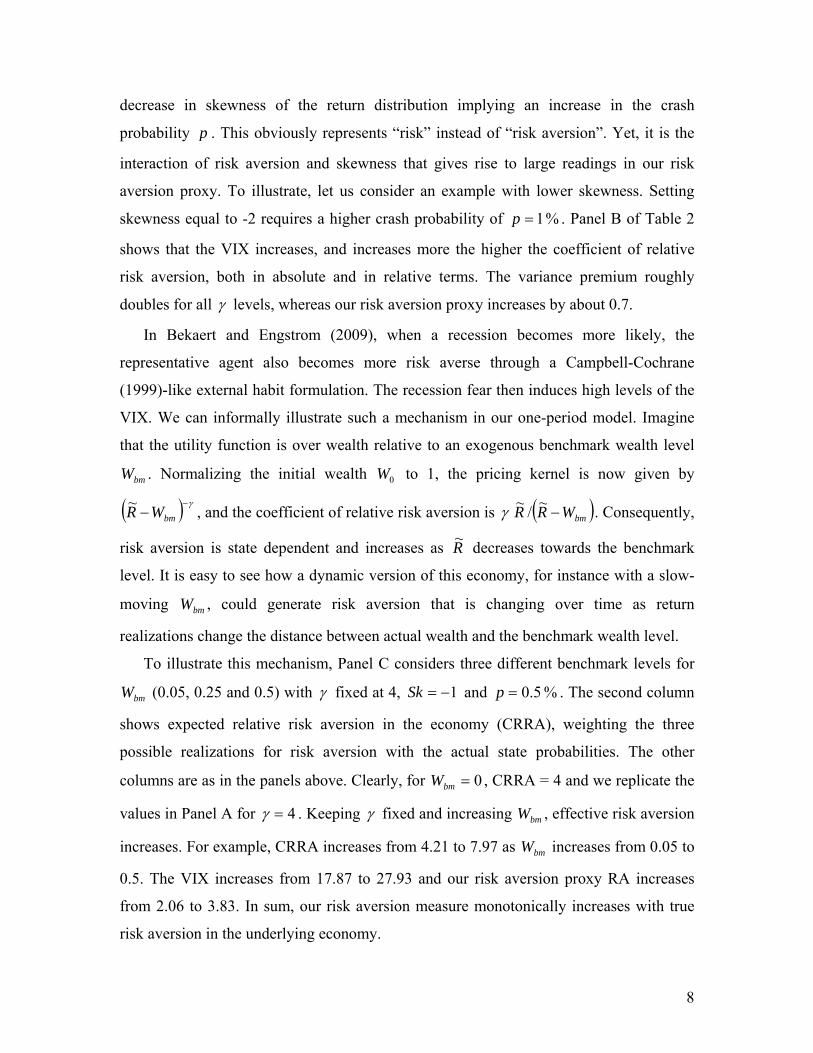
decrease in skewness of the return distribution implying an increase in the crash

probability p . This obviously represents “risk” instead of “risk aversion”. Yet, it is the

interaction of risk aversion and skewness that gives rise to large readings in our risk

aversion proxy. To illustrate, let us consider an example with lower skewness. Setting

skewness equal to -2 requires a higher crash probability of % 1p . Panel B of Table 2

shows that the VIX increases, and increases more the higher the coefficient of relative

risk aversion, both in absolute and in relative terms. The variance premium roughly

doubles for all levels, whereas our risk aversion proxy increases by about 0.7.

In Bekaert and Engstrom (2009), when a recession becomes more likely, the

representative agent also becomes more risk averse through a Campbell-Cochrane

(1999)-like external habit formulation. The recession fear then induces high levels of the

VIX. We can informally illustrate such a mechanism in our one-period model. Imagine

that the utility function is over wealth relative to an exogenous benchmark wealth level

. Normalizing the initial wealth to 1, the pricing kernel is now given by bmW

R

0W

bmW

bmW~

, and the coefficient of relative risk aversion is RR ~/

~ . Consequently,

risk aversion is state dependent and increases as R~

decreases towards the benchmark

level. It is easy to see how a dynamic version of this economy, for instance with a slow-

moving , could generate risk aversion that is changing over time as return

realizations change the distance between actual wealth and the benchmark wealth level.

bmW

To illustrate this mechanism, Panel C considers three different benchmark levels for

(0.05, 0.25 and 0.5) with bmW fixed at 4, 1Sk and % 5.0p . The second column

shows expected relative risk aversion in the economy (CRRA), weighting the three

possible realizations for risk aversion with the actual state probabilities. The other

columns are as in the panels above. Clearly, for 0bmW , CRRA = 4 and we replicate the

values in Panel A for 4 . Keeping fixed and increasing , effective risk aversion

increases. For example, CRRA increases from 4.21 to 7.97 as increases from 0.05 to

0.5. The VIX increases from 17.87 to 27.93 and our risk aversion proxy RA increases

from 2.06 to 3.83. In sum, our risk aversion measure monotonically increases with true

risk aversion in the underlying economy.

bmW

bmW

8

III. Risk, Uncertainty and Monetary Policy

We begin our analysis with a four-variable VAR on risk aversion, uncertainty, a measure

of monetary policy, and a business cycle indicator, using monthly data for the United

States from January 1990 (the start of the model-free VIX series) to July 2007. We

exclude recent data on the crisis, which presents special challenges. Table 1 describes all

the variables we use and assigns them a short-hand label.

To measure the monetary policy stance, we use the real interest rate (RERA), i.e., the

Fed funds end-of-the-month target rate minus the CPI inflation rate. In Section IV, we

consider alternative measures of the monetary policy stance for robustness. The

robustness analysis also includes a standard VAR specification featuring the nominal Fed

funds rate as the measure of monetary policy stance and price level measures (consumer

and producer price indices) as separate variables.

It is conceivable that the intriguing links between the VIX and monetary policy

simply reflect monetary policy and implied volatility jointly reacting to business cycle

conditions. For example, news indicating weaker than expected growth in the economy

may make a cut in the Fed funds target rate more likely, but at the same time cause

people to be effectively more risk averse, for example because a larger number of

households feel more constrained in their consumption relative to “habit,” or because

people fear a more uncertain future. To analyze business cycle effects, denoted by bct, we

use the log-difference of non-farm employment (DEMP) in our benchmark VAR.

While our main focus is on the links between risk, uncertainty and monetary policy,

our analysis may also provide important inputs to a rapidly growing macroeconomic

literature linking business cycles to the stock market. Beaudry and Portier (2006), for

example, present empirical evidence suggesting that business cycle fluctuations may be

driven to a large extent by changes in stock market expectations, which anticipate total

factor productivity movements. Bloom (2009) shows that “economic uncertainty” has

real effects, in particular it generates a sharp drop in employment and output, which

rebounds in the medium term, and a mild long-run overshoot. He explains these facts in

the context of a production model where uncertainty increases the region of inaction in

hiring and investment decisions of firms facing non-convex adjustment costs. In his

empirical work, Bloom uses the VIX index to create an index of “exogenous” volatility

9

shocks. However, as the VIX reflects both uncertainty and risk aversion, it is conceivable

that it is the risk aversion component of the VIX index that generates the real effects, not

the economic uncertainty component. Moreover, these shocks may be simply correlated

with business cycles, as predicted by external habit models, for example.6 In a recent

Economist article, Blanchard (2009) describes the VIX index as an indicator of Knightian

uncertainty, arguing that such uncertainty may prolong the current crisis. In both cases,

the implication is that monetary policy may want to respond strongly to uncertainty

shocks, in Bloom’s case to economic uncertainty shocks, in Blanchard’s case to what we

call risk aversion shocks.

We collect the four variables in the vector Zt = [bct, mpt, rat uct]' where bct is a

business cycle indicator, mpt is a measure of monetary policy stance, and rat and uct are

our risk aversion and uncertainty proxies, RA and UC. Without loss of generality, we

ignore constants. Consider the following structural VAR:

A Zt = Φ Zt-1 + εt (9)

where A is a 4x4 full-rank matrix and E[εt εt'] = I. Of main interest are the dynamic

responses to the structural shocks εt.

Of course, we start by estimating the reduced-form VAR:

Zt = B Zt-1 + C εt (10)

where B denotes A-1 Φ and C denotes A-1. Moreover, let us define Σ to be the variance-

covariance matrix of the reduced-form residuals, i.e., Σ = E[(C εt) (C εt)'] = C C'.

The first-order VAR in Equations (9) and (10) is useful to illustrate the identification

problem: Equation (10) yields 26 coefficients in the matrices B and Σ, but Equation (9)

has 32 unknowns. Hence, we need 6 restrictions on the VAR to identify the system. In

general, for a VAR of order k with N variables, we have (k+1)N2 parameters to identify

and we can estimate kN2 + N(N+1)/2 parameters. Hence, we need N(N-1)/2 restrictions

to identify the system. We later use formal selection criteria to select the correct order of

the VAR.

Reduced-form Statistics

Before we explore structural identification, Table 3 reports some reduced-form VAR

statistics. Panel A produces three lag-selection criteria: Akaike (AIC), Hannan-Quinn 6 To be fair, Bloom (2009) attempts to identify exogenous shocks to the VIX, which are less likely to be of a cyclical nature.

10

(HQIC) and Schwarz (SBIC). While the Schwarz criterion selects a VAR with one lag,

the AIC and HQIC criteria both select a VAR with three lags. We focus the remainder of

the analysis in this section on the three-lag VAR. Panel B reports Granger causality tests.

We find strong overall Granger causality in the risk aversion and real interest rate

equations. While significance is high for all the variables in the risk aversion equation,

monetary policy has the strongest effect. In the real rate equation, employment and

uncertainty are significant at 5% and 10% level, respectively. Granger causality is not

significantly present in either the employment or uncertainty equations. The strongest

relation is risk aversion predicting or anticipating employment significantly at the 5%

level. The real rate predicts or anticipates employment and uncertainty (both at the 10%

significance level).7

Finally, Panel C reports some specification tests on the residuals of the VAR. These

tests (see Johansen (1995)) test for autocorrelation in the residuals of the VAR at lag j

(j=1,2,3). The VAR with 3 lags clearly eliminates all serial correlation in the residuals.

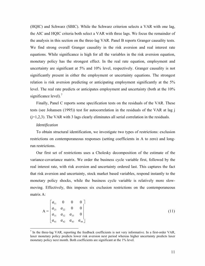
Identification

To obtain structural identification, we investigate two types of restrictions: exclusion

restrictions on contemporaneous responses (setting coefficients in A to zero) and long-

run restrictions.

Our first set of restrictions uses a Cholesky decomposition of the estimate of the

variance-covariance matrix. We order the business cycle variable first, followed by the

real interest rate, with risk aversion and uncertainty ordered last. This captures the fact

that risk aversion and uncertainty, stock market based variables, respond instantly to the

monetary policy shocks, while the business cycle variable is relatively more slow-

moving. Effectively, this imposes six exclusion restrictions on the contemporaneous

matrix A:

A = (11)

44434241

333231

2221

11

0

00

000

aaaa

aaa

aa

a

7 In the three-lag VAR, reporting the feedback coefficients is not very informative. In a first-order VAR, laxer monetary policy predicts lower risk aversion next period whereas higher uncertainty predicts laxer monetary policy next month. Both coefficients are significant at the 1% level.

11

The other set of restrictions combines five contemporaneous restrictions (also

imposed under the Cholesky decomposition above) with the assumption that monetary

policy has no long-run effect on the level of employment. This long-run restriction is

inspired by the literature on long-run money neutrality: money should not have a long run

effect on real variables. Bernanke and Mihov (1998b) and King and Watson (1992)

marshal empirical evidence in favor of money neutrality using data on money growth and

output growth.

Following Blanchard and Quah (1989), the model with a long-run restriction (LR)

involves a long-run response matrix, denoted by D:

D (I - B)-1 C. (12)

It follows that D D' = (I - B)-1 C C' [(I - B)-1]' = (I - B)-1 Σ [(I - B)-1]'. Hence, using the

estimates of B and Σ from the reduced-form VAR, we obtain D, and thus A-1 = C.8 The

system with five contemporaneous restrictions and one long-run exclusion restriction

corresponds to the following contemporaneous matrix A and long-run matrix D:

A = (13)

44434241

333231

2221

1211

0

00

00

aaaa

aaa

aa

aa

D = (14)

44434241

34333231

24232221

141311 0

dddd

dddd

dddd

ddd

Recently, the use of long-run restrictions to identify VARs has come under attack

(see, for example, Chari, Kehoe and McGrattan (2008)). However, Christiano,

Eichenbaum and Vigfusson (2006) show that many of the problems can be overcome by

using long-run information (rather than a parsimonious VAR) to identify the long-run

restrictions. Although they advocate using a non-parametrically estimated spectral

density matrix, a VAR with a relatively long lag-length effectively uses long-run

information to identify the restrictions. We therefore also checked that our results remain

8 To facilitate interpretation of the impulse responses, we adopt a sign normalization requiring that the diagonal elements of A-1 be positive.

12

robust to the use of a longer VAR lag-length. We did not go beyond four lags, as

otherwise the saturation ratio (data points to parameters) drops below 10.9

Both identification schemes satisfy necessary and sufficient conditions for global

identification of structural vector autoregressive systems (see Rubio-Ramírez, Waggoner

and Zha (2009)). Importantly, we consider various alternative identification schemes in

Section IV.

Structural Evidence

We couch our main results in the form of impulse-response functions (IRFs

henceforth), estimated in the usual way. We compute 90% bootstrapped confidence

intervals based on 1000 replications, and focus our discussion on significant responses.

We report the resulting structural impulse-response functions in Figure 3.

A one standard deviation negative shock to the real rate corresponds to a 33 basis

points decrease in both models. It lowers risk aversion by 0.05 after 4 months in the

model with contemporaneous restrictions and by 0.04 after 5 months in the model with

contemporaneous/long-run restrictions. The impact reaches a maximum of 0.09 after 12

and 17 months, respectively. It remains significant up and till lag 34 in the model with

contemporaneous restrictions and till lag 39 in the model with contemporaneous/long-run

restrictions. So, laxer monetary policy lowers risk aversion under both identification

schemes. The impact of a one standard deviation positive shock to risk aversion

(equivalent to 0.33 in both models) on the real rate is mostly negative but not statistically

significant.

A positive shock to the real rate lowers uncertainty in the short-run (between lags 0

and 3) but increases it in the medium-run (between lags 25 and 39 in the model with

contemporaneous restrictions and 29 - 42 in the model with contemporaneous/long-run

restrictions). The maximum positive impact is 0.04 at lag 25 and 0.05 at lag 29 in the

models with contemporaneous and contemporaneous/long-run restrictions, respectively.

In the other direction, the real rate decreases in the short-run following a positive one

standard deviation shock to uncertainty (equivalent to 0.50). In both models, the impact is

only statistically significant in periods 0 and 1, and it is about 5 basis points in period 1.

9 We also estimated a VAR with 1 lag, as selected by the Schwarz (SBIC) criterion. Our results were unaltered.

13

Hence, while uncertainty appears to have a structural effect on the subsequent monetary

policy stance, the effect is statistically weak.

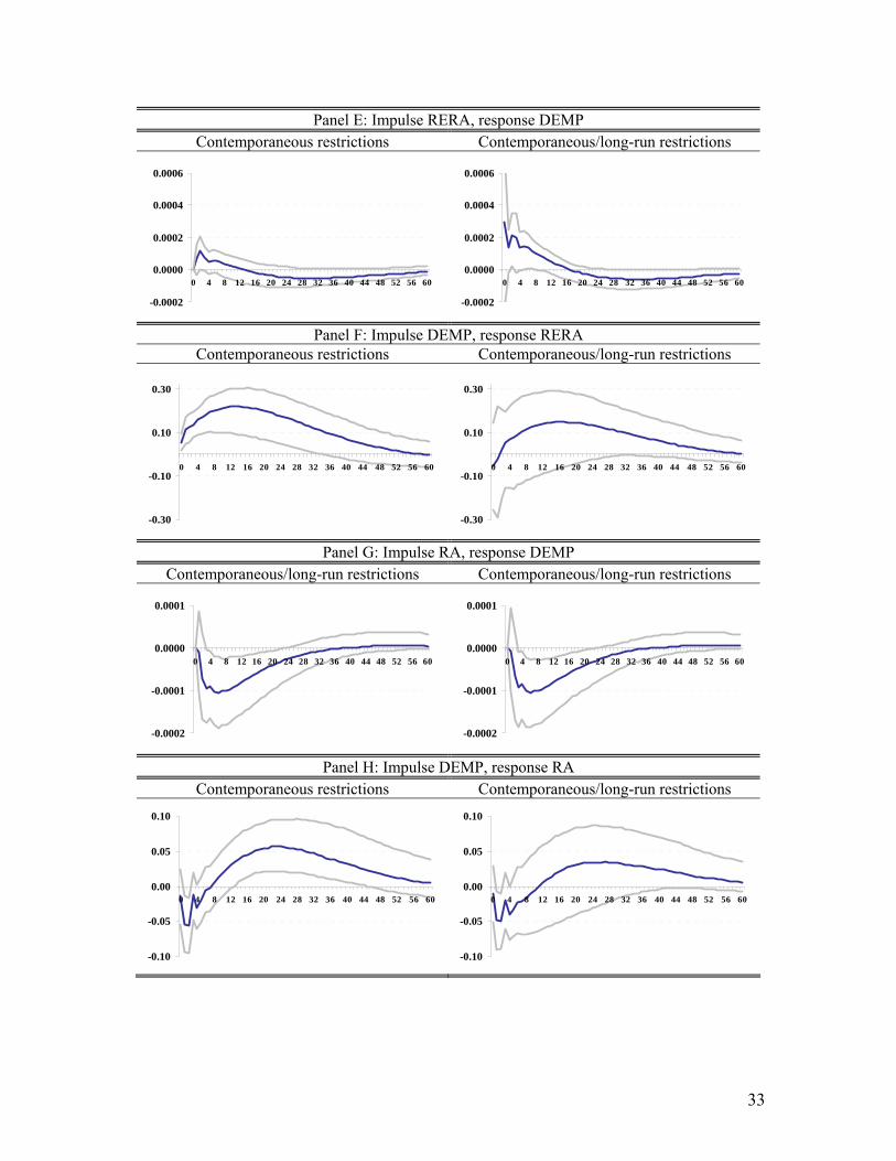
As for interactions with the business cycle variable (Panels E - J), a contractionary

monetary policy shock leads to a decline in employment growth after about 28 (23)

months, with the effect being (borderline) significant up and till lag 47 (57) in the model

with contemporaneous restrictions (contemporaneous/long-run restrictions). In the other

direction, monetary policy reacts as expected to business cycle fluctuations: a one

standard deviation positive shock to employment growth, equivalent to 0.0009, leads to a

higher real rate. Specifically, in the model with contemporaneous restrictions, the real

rate increases by a maximum of 22 basis points after 13 months, with the impact being

significant between lags 0 and 33. The impact is also positive in the model with

contemporaneous/long-run restrictions, and it is (borderline) statistically significant

between lags 29 and 38. Higher risk aversion decreases employment growth in both

models (Panel G). In the other direction, higher employment growth decreases risk

aversion in the short-run (between lags 1 and 2). Such effect is consistent with habit-

based theories of countercyclical risk aversion as in Campbell and Cochrane (1999).

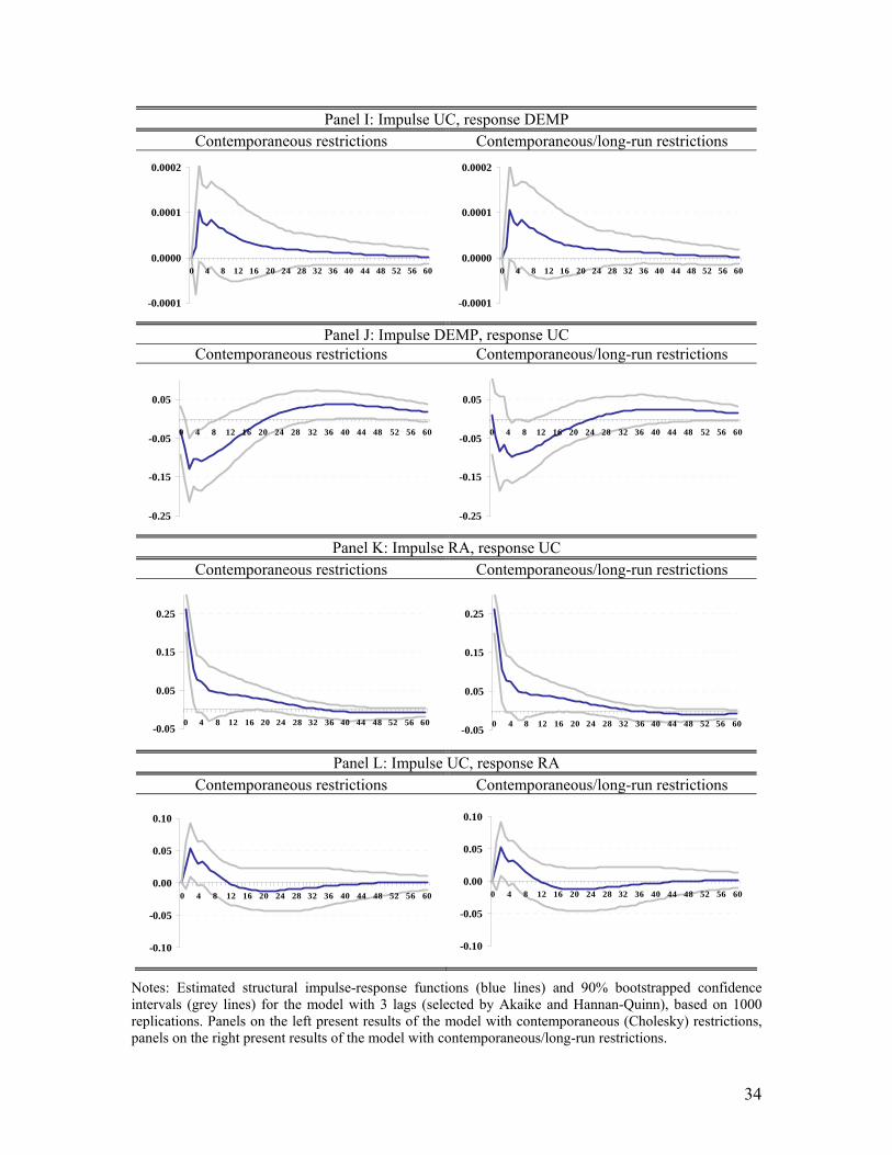
While positive uncertainty shocks do not have a statistically significant impact on

employment growth, higher employment growth has a negative effect on uncertainty in

the short-run (between lags 2 and 9 in the model with contemporaneous restrictions and

between lags 5 and 10 in the model with contemporaneous/long-run restrictions). These

results potentially shed new light on the analysis in Bloom (2009), who found that

uncertainty shocks generate significant business cycle effects, using the VIX as a

measure of uncertainty. Our results suggest that the link between the VIX and the

business cycle may well be driven by the risk aversion rather than the uncertainty

component of the VIX.10

Finally, increases in risk aversion predict future increases in uncertainty under both

identification schemes (Panel L). Uncertainty has a positive, albeit short-lived effect on

risk aversion (Panel K).

10 Popescu and Smets (2009) analyze the business cycle behavior of measures of perceived uncertainty and financial risk premia in Germany. They also find that financial risk aversion shocks are more important in driving business cycles than uncertainty shocks. Gilchrist and Zakrajšek (2011) document that innovations to the excess corporate bond premium, a proxy for the time-varying price of default risk, cause large and persistent contractions in economic activity.

14

Our main result is that monetary policy has a medium-run statistically significant

effect on risk aversion. This effect is not only statistically but also economically

significant. In Figure 4, we show what fraction of the structural variance of the four

variables in the VAR is due to monetary policy shocks. They account for over 30% of the

variance of risk aversion at horizons longer than 24 months in the model with

contemporaneous restrictions, and for over 40% of the variance of risk aversion at

horizons longer than 28 months in the model with contemporaneous/long-run restrictions.

IV. Robustness

In this section, we consider five types of robustness checks: 1) measurement of the

monetary policy stance; 2) measurement of the business cycle variable; 3) identification

of monetary policy shocks; 4) identification of uncertainty shocks; and 5) general

identification.

Measuring Monetary Policy

Our first alternative measure of the monetary policy stance is the Taylor rule residual,

i.e., the difference between the nominal Fed funds rate and the Taylor rule rate (TR rate).

The TR rate is estimated as in Taylor (1993):

TRt = Inft + NatRatet + 0.5*(Inft - TargInf) + 0.5*OGt (15)

where Inf is the annual inflation rate, NatRate is the “natural” real Fed funds rate

(consistent with full employment), which Taylor assumed to be 2%, TargInf is a target

inflation rate, also assumed to be 2%, and OG (output gap) is the percentage deviation of

real GDP from potential GDP. As additional measures of the monetary policy stance, we

consider the nominal Fed funds rate instead of the real rate, and (the growth rate of) the

monetary aggregate M1, which is commonly assumed to be under tight control of the

central bank.11 When we estimate a VAR with M1 in levels, we also use employment

instead of employment growth.

Table 4 reports summary statistics on the interaction of monetary policy with risk

aversion (Panel A) and with uncertainty (Panel B). The results confirm that looser

monetary policy stance lowers risk aversion in the short to medium run. This effect is

persistent, lasting for about two years. Risk aversion has no statistically significant effect

11 We consider the negative of the M1 (growth) so that a positive shock to this variable corresponds to monetary policy tightening, in line with all other measures of monetary policy we use.

15

on monetary policy. As for the effect of monetary policy on uncertainty, monetary

tightening increases uncertainty in the medium run. In the other direction, higher

uncertainty leads to laxer monetary policy in all specifications. The statistical

significance of the last two effects is less robust.

Measuring Business Cycle Variation

We consider the log-difference of industrial production, the log-difference of hours

worked and the level of jobless claims as alternative business cycle indicators. Unlike

employment, industrial production and hours worked, jobless claims is a stationary

variable, implying that VAR shocks do not have a long run effect on it. Our long-run

restriction on the effect of monetary policy is thus stronger when applied to jobless

claims: it restricts the total effect of monetary policy on jobless claims to be zero.

Nevertheless, our main results from Section III are confirmed for each specification with

an alternative business cycle variable. Detailed results are available upon request.

Identification of Monetary Policy Shocks

To check robustness with respect to the identification of monetary policy shocks, we

consider two specifications in which the Fed funds rate and the price level variable enter

separately (rather than jointly through the real interest rate). We estimate a five-variable

VAR with the consumer price index (CPI), employment, Fed funds rate, risk aversion and

uncertainty and a six-variable VAR adding the producer price index (PPI) to the above

list.12 To identify monetary policy shocks, we use a Cholesky ordering with CPI and

employment ordered first, followed by the Fed funds rate and PPI (in the six-variable

VAR), with risk aversion and uncertainty ordered last. This strategy follows Christiano,

Eichenbaum and Evans (1999).

We present impulse-responses to monetary policy shocks in Figure 5. A positive

monetary policy shock corresponds to a 16 basis points increase in the Fed funds rate in

both specifications. A contractionary monetary shock leads to a decrease in the CPI after

3 months in both models. The effect is significant up and till lag 16 and lag 25 in the

model with CPI and CPI/PPI, respectively. Furthermore, employment declines following

12 We estimate both models with four lags, as suggested by the Akaike criterion. All variables are in logarithms except for the Fed funds rate. Note that employment now also enters the VAR in levels.

16

a monetary contraction, although this effect is only statistically significant in the model

with CPI (after about 30 months).

Importantly, the reactions of both risk aversion and uncertainty are remarkably

similar to those uncovered in the previous section. Risk aversion decreases following a

monetary easing in both specifications. The effect reaches a maximum at lag 16 and 15 in

the model with CPI and CPI/PPI, respectively, and remains statistically significant till lag

24 and 28. The effects remain economically important as monetary policy shocks account

for over 16% (26%) of the variance of risk aversion at horizons longer than 30 months in

the model with CPI (CPI/PPI), see Figure 6. As for uncertainty, a higher Fed funds rate

lowers uncertainty in the short-run (between lags 2 and 14 in the model with CPI and

between lags 2 and 10 in the model with CPI/PPI). However, in the medium-run,

uncertainty increases in the model with CPI/PPI, which is also consistent with our

previous findings.

Identification of Uncertainty Shocks

As an alternative to our identification of uncertainty shocks, we follow Bloom (2009).

We construct an indicator of large, “exogenous” uncertainty shocks, i.e., a 0-1 variable

which takes on a value of one if uncertainty is more than 1.65 standard deviations above

the Hodrick Prescott (HP) detrended (λ = 129,600) mean of the uncertainty series and

zero otherwise. We isolate five shocks during our sample period. They are associated

with terror, war and financial crises.13 When uncertainty is above its mean for several

consecutive months, we assign a value of one to the chronologically first month in which

uncertainty was high and zero to the other months. The idea is that a high reading of

uncertainty in the first month represents an initial shock, while the remaining high values

reflect propagation of the initial shock. We then estimate a four-variable system with four

lags (as selected by the Akaike criterion), imposing contemporaneous restrictions, with

the uncertainty indicator ordered first, followed by employment, the real interest rate and

risk aversion. We also estimate a five-variable model, which includes the CPI, using the

following Cholesky ordering: uncertainty indicator, CPI, employment, Fed funds rate and

risk aversion.

13 The five events are: first Gulf war (August 1990), Asian crisis (October 1997), Russian/LTCM crisis (August 1998), 9/11 terrorist attack (September 2001), Corporate scandals (July 2002).

17

We present impulse-responses to such uncertainty shocks in Figure 7. The interest

rate decreases following a positive shock to uncertainty, with the effect being statistically

significant until lag 12 and 19 in the two respective models. It reaches a maximum

decrease of 10 basis points at lag 5 in the model with the real rate and 11 basis points at

lag 10 in the model with the Fed funds rate/CPI. Consequently, this identification scheme

leads to stronger, longer-lasting effects of uncertainty on monetary policy. As in the

previous section, higher uncertainty leads to higher risk aversion in the short-run.

Uncertainty shocks do not have a statistically significant impact on employment.

General Identification

We tried alternative identification schemes, while always preserving a structure that

satisfies necessary and sufficient conditions for global identification. For Cholesky

decompositions, we reversed the order of risk aversion and uncertainty in all our VARs,

and employment and CPI in our 5- and 6-variable VARs. We experimented with

imposing solely long-run restrictions, as well as with alternative combinations of

contemporaneous and long-run restrictions. We consistently found that looser monetary

policy lowers risk aversion in the medium-run. Results are available upon request.

We conclude that a lax monetary policy decreases risk aversion significantly, with the

effect being most pronounced in the medium run, while the interest rate tends to decrease

in response to high uncertainty. So, our previous results are robust to alternative ways of

identifying monetary policy and uncertainty shocks, and to other variations in

identification.

V. Channels

We have unearthed some intriguing interactions between the component in the VIX index

not related to actual stock market volatility, and the stance of monetary policy. If

monetary policy indeed affects risk aversion, our results could be important in the current

debate about the origins of the 2007-2009 crisis. While pinpointing in detail how

monetary policy affects risk aversion is beyond the scope of the article, we use this

section to empirically analyze some potential channels, discussed in a number of recent

articles.

18

Adrian and Shin (2008) suggest that the link between monetary policy and asset

prices runs through the balance sheets of financial intermediaries and that repo growth

rates adequately proxy for the riskiness of balance sheets. Using US data, they find that

the growth of outstanding repos forecasts the difference between implied and realized

volatility and that rapid growth in repos is associated with loose monetary policy (defined

as the Fed funds rate).14

To examine the Adrian-Shin channel in our structural framework, we use a four-

variable VAR as in Section III but with repo growth replacing the business cycle

variable. First, we examine whether introduction of this variable eliminates the effect of

the real interest rate on risk aversion we uncovered in the previous section. Table 5, Panel

A summarizes the results. Lax monetary policy is still associated with lower risk aversion

after 5 months. This effect is persistent. In the opposite direction, the responses are not

statistically significant. In Table 5, Panel B we investigate the interaction between the

real rate and uncertainty. Consistent with our previous findings, higher rates lower

uncertainty initially, while the real rate decreases following a positive shock to

uncertainty (though the latter effect is not statistically significant).

Second, we analyze the direct link between repo growth and risk aversion. Higher

repo growth has a negative effect on risk aversion but this effect is only statistically

significant in the model with contemporaneous restrictions (between lags 17 and 42). In

that specification, a shock to the real interest explains over 40% of the variance of risk

aversion beyond lag 25, while a repo shock explains not more than 6.5% at any of the 60

lags considered. In sum, our VAR suggests that the monetary policy – risk aversion link

does not only run through repo growth.

Many commentators have noted a rather large build up of liquidity through money

growth prior to financial crises (see also Adalid and Detken (2007), Alessi and Detken

(2009)). We thus use the growth rates of a broad money aggregate as a “channel”

variable, replacing the business cycle variable in the four-variable VAR. In particular, we

14 Adrian and Shin (2009) develop a simple equilibrium model in which financial intermediary balance sheets are the main engine for the determination of the price of risk in the economy, and short-term rates directly affect the risk-taking capacity of the financial sector. Brunnermeier and Sannikov (2010) similarly highlight equilibrium links between funding constraints in the financial sector, volatility dynamics and asset prices. Adrian, Moench and Shin (2010) document empirically that balance sheet variables play an important role in pricing the cross-section and time-series of asset prices.

19

consider the growth rate of M2 net of M1. This part of the money growth is arguably less

under control of a central bank and rather reflects activities in the financial sector.

Using this set-up, we confirm our finding that lower real rates lead to lower risk

aversion in both specifications considered (see Table 5, Panel A). We also confirm that

positive uncertainty shocks lower the real rate in the short-run (Table 5, Panel B). As for

the interaction between money growth and risk aversion, we find a structural link from

risk aversion to M2-M1: when risk aversion increases, M2-M1 increases in the short run.

This finding can be related to flights-to-safety effects in that risk-averse investors may

flee to relatively safe assets during crisis times. Such assets are incorporated in the M2

measure (e.g., money market and time deposits).

According to Borio and Lowe (2002), medium-term swings in asset prices are

associated with a rapid credit expansion. Moreover, they stress that such financial

imbalances may build up in a low inflation environment and that in some cases it is

appropriate for monetary policy to respond to these imbalances. Consequently, they

suggest a link between credit growth and monetary policy. It is conceivable that periods

of high risk appetite coincide with periods of rapid credit expansion, suggesting a channel

for the effect of monetary policy on risk aversion.

To investigate the role of credit, we consider two separate four-variable VAR

systems, with (private) credit growth and the first-difference of the credit-to-GDP ratio

replacing the business cycle variable. The significant impact of monetary policy on risk

aversion is present again (see Table 5, Panel A). Higher uncertainty decreases the real

rate in all specifications (see Table 5, Panel B). We do not find statistically significant

effects of credit developments on risk aversion in the stock market.

While our results are robust to two different identification schemes, one of them relies

on a long-run money neutrality assumption that is less palatable for our channel variables

than it is for the business cycle variable, to which it was applied in Section III. We

therefore examine an alternative identification scheme, using the Cholesky ordering with

CPI, a channel variable, the Fed funds rate, risk aversion and uncertainty. We

consistently find that looser monetary policy lowers risk aversion. In sum, considering

channels through which monetary policy may affect risk aversion does not eliminate the

direct effect of monetary policy on risk appetite.

20

VI. Conclusions

A number of recent studies point at a potential link between loose monetary policy and

excessive risk-taking in financial markets. Rajan (2006) conjectures that in times of

ample liquidity supplied by the central bank, investment managers have a tendency to

engage in risky, correlated investments. To earn excess returns in a low interest rate

environment, their investment strategies may entail risky, tail-risk sensitive and illiquid

securities (“search for yield”). Moreover, a tendency for herding behaviour emerges due

to the particular structure of managerial compensation contracts. Managers are evaluated

vis-à-vis their peers and by pursuing strategies similar to others, they can ensure that they

do not under perform. This “behavioral” channel of monetary policy transmission can

lead to the formation of asset prices bubbles and can threaten financial stability. Yet,

there is no empirical evidence on the links between risk aversion in financial markets and

monetary policy.

This article has attempted to provide a first characterization of the dynamic links

between risk, uncertainty and monetary policy, using a simple vector-autoregressive

framework. We decompose implied volatility into two components, risk aversion and

uncertainty, and find interactions between each of the components and monetary policy

to be rather different. Lax monetary policy increases risk appetite (decreases risk

aversion) in the future, with the effect lasting for about two years and starting to be

significant after five months. On the other hand, high uncertainty leads to laxer monetary

policy in the near-term future. These results are robust to controlling for business cycle

movements. Consequently, our VAR analysis provides a clean interpretation of the

stylized facts regarding the dynamic relations between the VIX and the monetary policy

stance depicted in Figure 1. The primary component driving the co-movement between

past monetary policy stance and current VIX levels (first column of Figure 1) is risk

aversion. The uncertainty component of the VIX lies behind the negative relation in the

opposite direction (second column of Figure 1).

We hope that our analysis will inspire further empirical work and research on the

exact theoretical links between monetary policy and risk-taking behavior in asset

markets. In particular, recent work in the consumption-based asset pricing literature

attempts to understand the structural sources of the VIX dynamics (see Bekaert and

21

Engstrom (2009), Bollerslev, Tauchen and Zhou (2008), Drechsler and Yaron (2009)).

Yet, none of these models incorporates monetary policy equations. In macroeconomics, a

number of articles have embedded term structure dynamics into the standard New-

Keynesian workhorse model (Bekaert, Cho, Moreno (2010), Rudebusch and Wu (2008)),

but no models accommodate the dynamic interactions between monetary policy, risk

aversion and uncertainty, uncovered in this article.

The policy implications of our work are potentially very important. Because monetary

policy significantly affects risk aversion and risk aversion significantly affects the

business cycle, we seem to have uncovered a monetary policy transmission mechanism

missing in extant macroeconomic models. Fed chairman Bernanke (see Bernanke (2002))

interprets his work on the effect of monetary policy on the stock market (Bernanke and

Kuttner (2005)) as suggesting that monetary policy would not have a sufficiently strong

effect on asset markets to pop a “bubble” (see also Bernanke and Gertler (2001), Gilchrist

and Leahy (2002), and Greenspan (2002)). However, if monetary policy significantly

affects risk appetite in asset markets, this conclusion may not hold. If one channel is that

lax monetary policy induces excess leverage as in Adrian and Shin (2008), perhaps

monetary policy is potent enough to weed out financial excess. Conversely, in times of

crisis and heightened risk aversion, monetary policy can influence risk aversion in the

market place, and therefore affect real outcomes.

22

REFERENCES

Adalid, R. and C. Detken (2007). “Liquidity Shocks and Asset Price Boom/Bust Cycles,” ECB Working Paper No. 732.

Adrian, T. and H. S. Shin (2008). “Liquidity, Monetary Policy, and Financial Cycles,” Current Issues in Economics and Finance 14 (1), Federal Reserve Bank of New York.

Adrian, T. and H. S. Shin (2009). “Financial Intermediaries and Monetary Economics,” Handbook of Monetary Economics, Chapter 12, ed. by Benjamin Friedman and Michael Woodford, forthcoming, pp. 601-650.

Adrian, T., E. Moench and H.S. Shin (2010). “Financial Intermediation, Asset Prices, and Macroeconomic Dynamics,” Federal Reserve Bank of New York Staff Report No. 422.

Alessi, L. and C. Detken (2009). “Real-time Early Warning Indicators for Costly Asset Price Boom/Bust Cycles - A Role for Global Liquidity,” ECB Working Paper No. 1039.

Altunbas, Y., L. Gambacorta and D. Marquéz-Ibañez (2010). “Does Monetary Policy Affect Bank Risk-taking?”, ECB Working Paper No. 1166.

Baker, M. and J. Wurgler (2007). “Investor Sentiment in the Stock Market,” Journal of Economic Perspectives 21, pp. 129-151.

Bakshi, G. and D. Madan (2000). “Spanning and Derivative-Security Valuation,” Journal of Financial Economics, Vol. 55 (2), pp. 205-238.

Bakshi, G., N. Kapadia and D. Madan (2003). “Stock Return Characteristics, Skew Laws, and Differential Pricing of Individual Equity Options,” Review of Financial Studies, Vol. 16 (1), pp. 101-143.

Barro, R.J. (2006). “Rare Disasters and Asset Markets in the Twentieth Century,” Quarterly Journal of Economics, Vol. 121 (3), pp. 823-866.

Beaudry, P. and F. Portier (2006). “Stock Prices, News, and Economic Fluctuations,” American Economic Review, Vol. 96 (4), pp. 1293-1307.

Bekaert, G., S. Cho and A. Moreno (2010). “New Keynesian Macroeconomics and the Term Structure,” Journal of Money, Credit and Banking, Vol. 42 (1), pp. 33-62.

Bekaert, G. and E. Engstrom (2009). “Asset Return Dynamics under Bad Environment-Good Environment Fundamentals,” working paper, Columbia GSB.

Bekaert, G., E. Engstrom, and Y. Xing (2009). “Risk, Uncertainty, and Asset Prices,” Journal of Financial Economics 91, pp. 59-82.

Bernanke, B. (2002). “Asset-Price ‘Bubbles’ and Monetary Policy,” speech before the New York chapter of the National Association for Business Economics, New York, New York, October 15.

23

Bernanke, B. and M. Gertler (2001). “Should Central Banks Respond to Movements in Asset Prices?” American Economic Review, 91 (May), pp. 253-57.

Bernanke, B. and K. Kuttner (2005). “What Explains the Stock Market’s Reaction to Federal Reserve Policy?” Journal of Finance, Vol. 60 (3), pp. 1221-1257.

Bernanke, B. and I. Mihov (1998a). “Measuring Monetary Policy,” Quarterly Journal of Economics, Vol. 113 (3), pp. 869-902.

Bernanke, B. and I. Mihov (1998b). “The Liquidity Effect and Long-run Neutrality,” Carnegie-Rochester Conference Series on Public Policy, Vol. 49 (1), pp. 149-194.

Blanchard, O. (2009). “Nothing to Fear but Fear Itself,” Economist, January 29.

Blanchard, O. and D. Quah (1989). “The Dynamic Effects of Aggregate Demand and Supply Disturbances,” American Economic Review Vol. 79 (4), pp. 655-73.

Bloom, N. (2009). “The Impact of Uncertainty Shocks,” Econometrica, Vol. 77, No. 3, pp. 623-685.

Bloom, N., M. Floetotto and N. Jaimovich (2009). “Real Uncertain Business Cycles,” working paper, Stanford University.

Bollerslev, T., G. Tauchen and H. Zhou (2009). “Expected Stock Returns and Variance Risk Premia,” Review of Financial Studies, Vol. 22, No. 11, pp. 4463-4492.

Borio, C. and P. Lowe (2002). “Asset Prices, Financial and Monetary Stability: Exploring the Nexus,” BIS Working Paper No. 114.

Borio, C. and H. Zhu (2008). “Capital Regulation, Risk-Taking and Monetary Policy: A Missing Link in the Transmission Mechanism?” BIS Working Paper No. 268.

Breeden, D. and R. Litzenberger (1978). “Prices of State-contingent Claims Implicit in Option Prices,” Journal of Business, Vol. 51, No. 4, pp. 621-651.

Brunnermeier, M. K. and Y. Sannikov (2010). “A Macroeconomic Model with a Financial Sector,” working paper, Princeton University.

Campbell, J. Y and J. Cochrane (1999). “By Force of Habit: A Consumption Based Explanation of Aggregate Stock Market Behavior,” Journal of Political Economy 107 (2), pp. 205-251.

Carr, P. and L. Wu (2009). “Variance Risk Premiums,” Review of Financial Studies. Vol. 22 (3), pp. 1311-1341.

Chicago Board Options Exchange (2004). “VIX CBOE Volatility Index,” White Paper.

24

Chari, V. V., P. Kehoe and E. McGrattan (2008). “Are Structural VARs with Long-run Restrictions Useful in Developing Business Cycle Theory?”, Journal of Monetary Economics 55 (8), pp. 1337-1352.

Christiano, L. J., M. Eichenbaum and C. L. Evans (1999). “Monetary Policy Shocks: What Have We Learned and to What End?” In J. B. Taylor and M. Woodford (eds.), Handbook of Macroeconomics, Vol. 1A, pp. 65-148, North-Holland.

Christiano, L. J., M. Eichenbaum and C. L. Evans (2005). “Nominal Rigidities and the Dynamic Effects of a Shock to Monetary Policy,” Journal of Political Economy, Vol. 113 (1), pp. 1-45.

Christiano, L. J., M. Eichenbaum and R. Vigfusson (2006). “Alternative Procedures for Estimating Vector Autoregressions Identified with Long-Run Restrictions,” Journal of the European Economic Association 4 (2-3), pp. 475-483.

Coudert, V. and M. Gex (2008). “Does Risk Aversion Drive Financial Crises? Testing the Predictive Power of Empirical Indicators,” Journal of Empirical Finance 15, pp. 167-184.

Drechsler, I. (2009). “Uncertainty, Time-Varying Fear, and Asset Prices,” working paper, Wharton School.

Drechsler, I. and A. Yaron (2009). “What’s Vol Got to Do with It,” working paper, Wharton School.

Gilchrist, S. and J.V. Leahy (2002). “Monetary Policy and Asset Prices,” Journal of Monetary Economics 49 (1), pp. 75-97.

Gilchrist, S. and E. Zakrajšek (2011). “Credit Spreads and Business Cycle Fluctuations,” working paper, Boston University and Federal Reserve Board.

Greenspan, A. (2002). “Economic Volatility,” speech before a symposium sponsored by the Federal Reserve Bank of Kansas City, Jackson Hole, Wyoming, August 30.

Ioannidou, V. P., S. Ongena and J.-L. Peydró (2009). “Monetary Policy, Risk-Taking and Pricing: Evidence from a Quasi Natural Experiment,” European Banking Center Discussion Paper No. 2009-04S.

Jiménez, G., S. Ongena, J.-L. Peydró and J. Saurina (2009). “Hazardous Times for Monetary Policy: What do Twenty-Three Million Bank Loans Say About the Effects of Monetary Policy on Credit Risk?”, CEPR Discussion Paper No. 6514.

Johansen, S. (1995). Likelihood-Based Inference in Coitegrated Vector Auto-Regressive Models. Oxford: Oxford University Press.

King, R. and M. W. Watson (1992). “Testing Long Run Neutrality,” NBER Working Papers No. 4156, National Bureau of Economic Research.

25

Maddaloni, A. and J.-L. Peydró (2010). “Bank Risk-Taking, Securitization, Supervision, and Low Interest Rates: Evidence from Lending Standards,” forthcoming in the Review of Financial Studies.

Popescu, A. and F. Smets (2009). “Uncertainty, Risk-taking and the Business Cycle,” mimeo, European Central Bank.

Rajan, R. (2006). “Has Finance Made the World Riskier?” European Financial Management 12 (4), pp. 499-533.

Rigobon, R. and B. Sack (2003). “Measuring the Reaction of Monetary Policy to the Stock Market,” Quarterly Journal of Economics 118 (2), pp. 639-669.

Rigobon, R. and B. Sack (2004). “The Impact of Monetary Policy on Asset Prices,” Journal of Monetary Economics 51 (8), pp. 1553-1575.

Rubio-Ramírez, J. F., D. F. Waggoner and T. Zha (2009). “Structural Vector Autoregressions: Theory of Identification and Algorithms for Inference,” forthcoming in the Review of Economic Studies.

Rudebusch, G. D. and T. Wu (2008). “A Macro-Finance Model of the Term Structure, Monetary Policy and the Economy,” Economic Journal 118 (530), pp. 906-926.

Sharpe, W. F. (1990). “Investor Wealth Measures and Expected Return,” Quantifying the Market Risk Premium Phenomenon for Investment Decision Making, The Institute of Chartered Financial Analysts, pp. 29-37.

Taylor, J. B. (1993). “Discretion Versus Policy Rules in Practice,” Carnegie-Rochester Conference Series on Public Policy 39, pp. 195–214.

Thorbecke, W. (1997). “On Stock Market Returns and Monetary Policy,” Journal of Finance 52 (2), pp. 635-654.

Whaley, R. E. (2000). “The Investor Fear Gauge,” Journal of Portfolio Management, Spring, pp. 12-17.

26

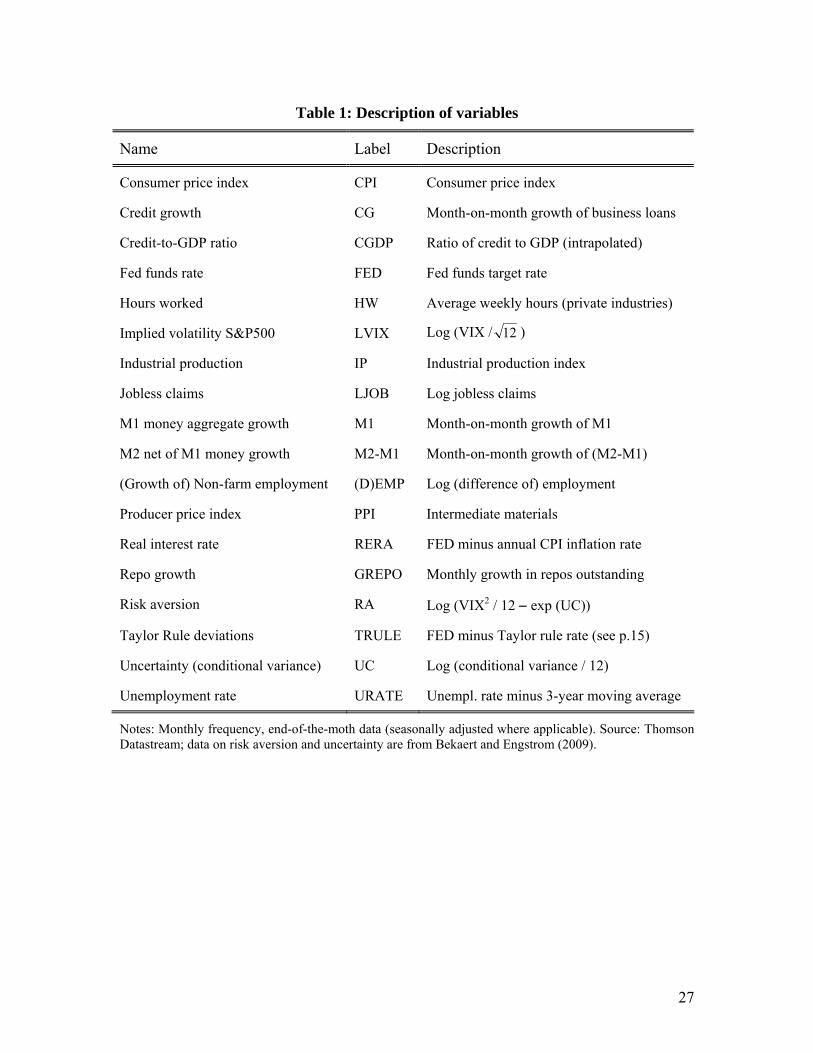
Table 1: Description of variables

Name Label Description

Consumer price index CPI Consumer price index

Credit growth CG Month-on-month growth of business loans

Credit-to-GDP ratio CGDP Ratio of credit to GDP (intrapolated)

Fed funds rate FED Fed funds target rate

Hours worked HW Average weekly hours (private industries)

Implied volatility S&P500 LVIX Log (VIX / 12 )

Industrial production IP Industrial production index

Jobless claims LJOB Log jobless claims

M1 money aggregate growth M1 Month-on-month growth of M1

M2 net of M1 money growth M2-M1 Month-on-month growth of (M2-M1)

(Growth of) Non-farm employment (D)EMP Log (difference of) employment

Producer price index PPI Intermediate materials

Real interest rate RERA FED minus annual CPI inflation rate

Repo growth GREPO Monthly growth in repos outstanding

Risk aversion RA Log (VIX2 / 12 exp (UC))

Taylor Rule deviations TRULE FED minus Taylor rule rate (see p.15)

Uncertainty (conditional variance) UC Log (conditional variance / 12)

Unemployment rate URATE Unempl. rate minus 3-year moving average

Notes: Monthly frequency, end-of-the-moth data (seasonally adjusted where applicable). Source: Thomson Datastream; data on risk aversion and uncertainty are from Bekaert and Engstrom (2009).

27

Figure 1: Cross-correlogram LVIX RERA

Notes: The first column presents the (lagged) cross-correlogram between the log of the VIX (LVIX) and past values of the real interest rate (RERA). The second column presents the (lead) cross-correlogram between LVIX and future values of RERA. Dashed vertical lines indicate 95% confidence intervals for the cross-correlation. The third column presents the cross-correlation values. The index i indicates the number of months either lagged or led for the real interest rate variable.

28

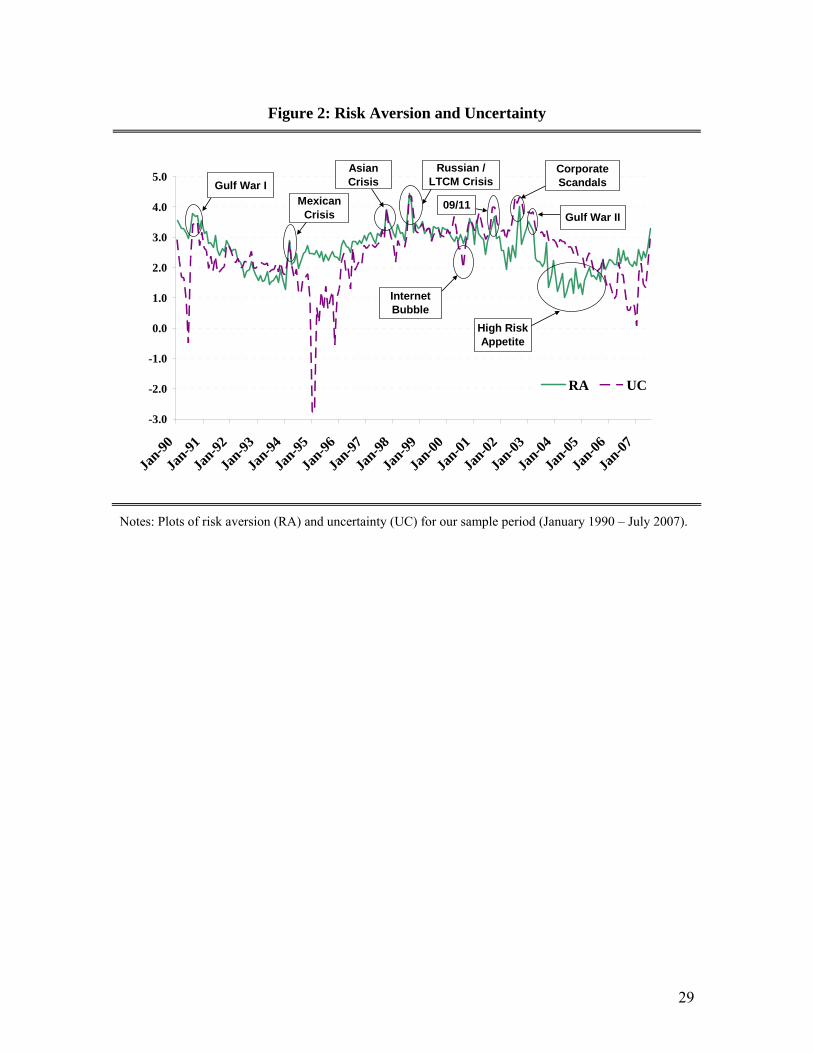
Figure 2: Risk Aversion and Uncertainty

-3.0

-2.0

-1.0

0.0

1.0

2.0

3.0

4.0

5.0

Jan-9

0

Jan-9

1

Jan-9

2

Jan-9

3

Jan-9

4

Jan-9

5

Jan-9

6

Jan-9

7

Jan-9

8

Jan-9

9

Jan-0

0

Jan-0

1

Jan-0

2

Jan-0

3

Jan-0

4

Jan-0

5

Jan-0

6

Jan-0

7

RA UC

AsianCrisis

Internet Bubble

Russian / LTCM Crisis

Corporate Scandals

High Risk Appetite

09/11

Gulf War I

Mexican Crisis Gulf War II

Notes: Plots of risk aversion (RA) and uncertainty (UC) for our sample period (January 1990 – July 2007).

29

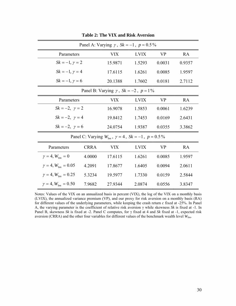
Table 2: The VIX and Risk Aversion

Panel A: Varying , 1Sk , % 5.0p

Parameters VIX LVIX VP RA

2,1 Sk 15.9871 1.5293 0.0031 0.9357

4,1 Sk 17.6115 1.6261 0.0085 1.9597

6,1 Sk 20.1388 1.7602 0.0181 2.7112

Panel B: Varying , 2Sk , % 1p

Parameters VIX LVIX VP RA

2,2 Sk 16.9078 1.5853 0.0061 1.6239

4,2 Sk 19.8412 1.7453 0.0169 2.6431

6,2 Sk 24.0754 1.9387 0.0355 3.3862

Panel C: Varying , bmW 4 , 1Sk , % 5.0p

Parameters CRRA VIX LVIX VP RA

0,4 bmW 4.0000 17.6115 1.6261 0.0085 1.9597

05.0,4 bmW 4.2091 17.8677 1.6405 0.0094 2.0611

25.0,4 bmW 5.3234 19.5977 1.7330 0.0159 2.5844

50.0,4 bmW 7.9682 27.9344 2.0874 0.0556 3.8347

Notes: Values of the VIX on an annualized basis in percent (VIX), the log of the VIX on a monthly basis (LVIX), the annualized variance premium (VP), and our proxy for risk aversion on a monthly basis (RA) for different values of the underlying parameters, while keeping the crash return c fixed at -25%. In Panel A, the varying parameter is the coefficient of relative risk aversion γ while skewness Sk is fixed at -1. In Panel B, skewness Sk is fixed at -2. Panel C computes, for γ fixed at 4 and Sk fixed at -1, expected risk aversion (CRRA) and the other four variables for different values of the benchmark wealth level Wbm.

30

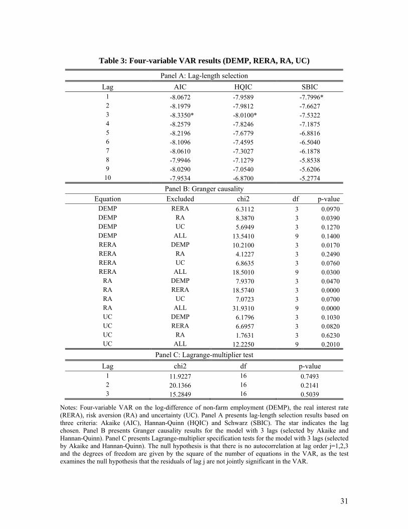
Table 3: Four-variable VAR results (DEMP, RERA, RA, UC)

Panel A: Lag-length selection

Lag AIC HQIC SBIC 1 -8.0672 -7.9589 -7.7996* 2 -8.1979 -7.9812 -7.6627 3 -8.3350* -8.0100* -7.5322 4 -8.2579 -7.8246 -7.1875 5 -8.2196 -7.6779 -6.8816 6 -8.1096 -7.4595 -6.5040 7 -8.0610 -7.3027 -6.1878 8 -7.9946 -7.1279 -5.8538 9 -8.0290 -7.0540 -5.6206

10 -7.9534 -6.8700 -5.2774

Panel B: Granger causality Equation Excluded chi2 df p-value

DEMP RERA 6.3112 3 0.0970 DEMP RA 8.3870 3 0.0390 DEMP UC 5.6949 3 0.1270 DEMP ALL 13.5410 9 0.1400 RERA DEMP 10.2100 3 0.0170 RERA RA 4.1227 3 0.2490 RERA UC 6.8635 3 0.0760 RERA ALL 18.5010 9 0.0300

RA DEMP 7.9370 3 0.0470 RA RERA 18.5740 3 0.0000 RA UC 7.0723 3 0.0700 RA ALL 31.9310 9 0.0000 UC DEMP 6.1796 3 0.1030 UC RERA 6.6957 3 0.0820 UC RA 1.7631 3 0.6230 UC ALL 12.2250 9 0.2010

Panel C: Lagrange-multiplier test

Lag chi2 df p-value 1 11.9227 16 0.7493 2 20.1366 16 0.2141 3 15.2849 16 0.5039

Notes: Four-variable VAR on the log-difference of non-farm employment (DEMP), the real interest rate (RERA), risk aversion (RA) and uncertainty (UC). Panel A presents lag-length selection results based on three criteria: Akaike (AIC), Hannan-Quinn (HQIC) and Schwarz (SBIC). The star indicates the lag chosen. Panel B presents Granger causality results for the model with 3 lags (selected by Akaike and Hannan-Quinn). Panel C presents Lagrange-multiplier specification tests for the model with 3 lags (selected by Akaike and Hannan-Quinn). The null hypothesis is that there is no autocorrelation at lag order j=1,2,3 and the degrees of freedom are given by the square of the number of equations in the VAR, as the test examines the null hypothesis that the residuals of lag j are not jointly significant in the VAR.

31

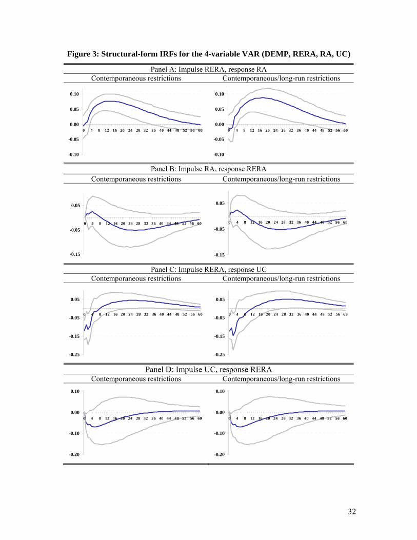
Figure 3: Structural-form IRFs for the 4-variable VAR (DEMP, RERA, RA, UC)

Panel A: Impulse RERA, response RA Contemporaneous restrictions Contemporaneous/long-run restrictions

-0.10

-0.05

0.00

0.05

0.10

0 4 8 12 16 20 24 28 32 36 40 44 48 52 56 60

-0.10

-0.05

0.00

0.05

0.10

0 4 8 12 16 20 24 28 32 36 40 44 48 52 56 60

Panel B: Impulse RA, response RERA Contemporaneous restrictions Contemporaneous/long-run restrictions

-0.15

-0.05

0.05

0 4 8 12 16 20 24 28 32 36 40 44 48 52 56 60

-0.15

-0.05

0.05

0 4 8 12 16 20 24 28 32 36 40 44 48 52 56 60

Panel C: Impulse RERA, response UC Contemporaneous restrictions Contemporaneous/long-run restrictions

-0.25

-0.15

-0.05

0.05

0 4 8 12 16 20 24 28 32 36 40 44 48 52 56 60

-0.25

-0.15

-0.05

0.05

0 4 8 12 16 20 24 28 32 36 40 44 48 52 56 60

Panel D: Impulse UC, response RERA Contemporaneous restrictions Contemporaneous/long-run restrictions

-0.20

-0.10

0.00

0.10

0 4 8 12 16 20 24 28 32 36 40 44 48 52 56 60

-0.20

-0.10

0.00

0.10

0 4 8 12 16 20 24 28 32 36 40 44 48 52 56 60

32

Panel E: Impulse RERA, response DEMP Contemporaneous restrictions Contemporaneous/long-run restrictions

-0.0002

0.0000

0.0002

0.0004

0.0006

0 4 8 12 16 20 24 28 32 36 40 44 48 52 56 60

-0.0002

0.0000

0.0002

0.0004

0.0006

0 4 8 12 16 20 24 28 32 36 40 44 48 52 56 60

Panel F: Impulse DEMP, response RERA Contemporaneous restrictions Contemporaneous/long-run restrictions

-0.30

-0.10

0.10

0.30

0 4 8 12 16 20 24 28 32 36 40 44 48 52 56 60

-0.30

-0.10

0.10

0.30

0 4 8 12 16 20 24 28 32 36 40 44 48 52 56 60

Panel G: Impulse RA, response DEMP Contemporaneous/long-run restrictions Contemporaneous/long-run restrictions

-0.0002

-0.0001

0.0000

0.0001

0 4 8 12 16 20 24 28 32 36 40 44 48 52 56 60

-0.0002

-0.0001

0.0000

0.0001

0 4 8 12 16 20 24 28 32 36 40 44 48 52 56 60

Panel H: Impulse DEMP, response RA Contemporaneous restrictions Contemporaneous/long-run restrictions

-0.10

-0.05

0.00

0.05

0.10

0 4 8 12 16 20 24 28 32 36 40 44 48 52 56 60

-0.10

-0.05

0.00

0.05

0.10

0 4 8 12 16 20 24 28 32 36 40 44 48 52 56 60

33

Panel I: Impulse UC, response DEMP Contemporaneous restrictions Contemporaneous/long-run restrictions

-0.0001

0.0000

0.0001

0.0002

0 4 8 12 16 20 24 28 32 36 40 44 48 52 56 60

-0.0001

0.0000

0.0001

0.0002

0 4 8 12 16 20 24 28 32 36 40 44 48 52 56 60

Panel J: Impulse DEMP, response UC Contemporaneous restrictions Contemporaneous/long-run restrictions

-0.25

-0.15

-0.05

0.05

0 4 8 12 16 20 24 28 32 36 40 44 48 52 56 60

-0.25

-0.15

-0.05

0.05

0 4 8 12 16 20 24 28 32 36 40 44 48 52 56 60

Panel K: Impulse RA, response UC Contemporaneous restrictions Contemporaneous/long-run restrictions

-0.05

0.05

0.15

0.25

0 4 8 12 16 20 24 28 32 36 40 44 48 52 56 60

-0.05

0.05

0.15

0.25

0 4 8 12 16 20 24 28 32 36 40 44 48 52 56 60

Panel L: Impulse UC, response RA Contemporaneous restrictions Contemporaneous/long-run restrictions

-0.10

-0.05

0.00

0.05

0.10

0 4 8 12 16 20 24 28 32 36 40 44 48 52 56 60

-0.10

-0.05

0.00

0.05

0.10

0 4 8 12 16 20 24 28 32 36 40 44 48 52 56 60

Notes: Estimated structural impulse-response functions (blue lines) and 90% bootstrapped confidence intervals (grey lines) for the model with 3 lags (selected by Akaike and Hannan-Quinn), based on 1000 replications. Panels on the left present results of the model with contemporaneous (Cholesky) restrictions, panels on the right present results of the model with contemporaneous/long-run restrictions.

34

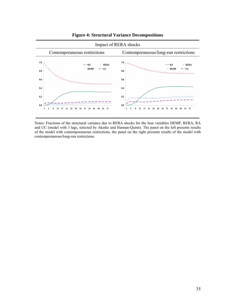
Figure 4: Structural Variance Decompositions

Impact of RERA shocks

Contemporaneous restrictions Contemporaneous/long-run restrictions

0.0

0.2

0.4

0.6

0.8

1.0

1 5 9 13 17 21 25 29 33 37 41 45 49 53 57

RA RERA

DEMP UC

0.0

0.2

0.4

0.6

0.8

1.0

1 5 9 13 17 21 25 29 33 37 41 45 49 53 57

RA RERA

DEMP UC

Notes: Fractions of the structural variance due to RERA shocks for the four variables DEMP, RERA, RA and UC (model with 3 lags, selected by Akaike and Hannan-Quinn). The panel on the left presents results of the model with contemporaneous restrictions, the panel on the right presents results of the model with contemporaneous/long-run restrictions.

35

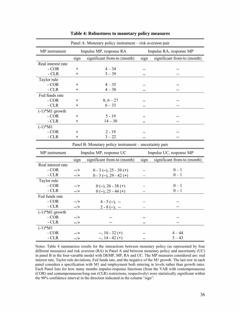
Table 4: Robustness to monetary policy measures

Panel A: Monetary policy instrument – risk aversion pair

MP instrument Impulse MP, response RA Impulse RA, response MP

sign significant from-to (month) sign significant from-to (month) Real interest rate

- COR - CLR

+ +

4 – 34 5 – 39

-- --

Taylor rule - COR - CLR

+ +

4 – 35 4 – 38

-- --

Fed funds rate - COR - CLR

+ +

0, 6 – 27

6 – 33

-- --

(-1)*M1 growth - COR - CLR

+ +

5 - 19

14 – 30

-- --

(-1)*M1 - COR - CLR

+ +

2 - 19 3 – 22

-- --

Panel B: Monetary policy instrument – uncertainty pair

MP instrument Impulse MP, response UC Impulse UC, response MP

sign significant from-to (month) sign significant from-to (month) Real interest rate

- COR - CLR

/+ /+

0 - 3 (), 25 - 39 (+) 0 - 3 (), 29 - 42 (+)

0 – 1 0 – 1

Taylor rule - COR - CLR

/+ /+

0 (), 26 - 38 (+) 0 (), 25 - 44 (+)

0 – 1 0 – 1

Fed funds rate - COR - CLR

/+ /+

4 - 5 (), -- 2 - 8 (), --

-- --

(-1)*M1 growth - COR - CLR

/+ /+

-- --

-- --

(-1)*M1 - COR - CLR

/+ /+

--, 10 - 32 (+) --, 14 - 42 (+)

4 – 44 5 – 43

Notes: Table 4 summarizes results for the interactions between monetary policy (as represented by four different measures) and risk aversion (RA) in Panel A and between monetary policy and uncertainty (UC) in panel B in the four-variable model with DEMP, MP, RA and UC. The MP measures considered are: real interest rate, Taylor rule deviations, Fed funds rate, and the negative of the M1 growth. The last row in each panel considers a specification with M1 and employment both entering in levels rather than growth rates. Each Panel lists for how many months impulse-response functions (from the VAR with contemporaneous (COR) and contemporaneous/long-run (CLR) restrictions, respectively) were statistically significant within the 90% confidence interval in the direction indicated in the column “sign”.

36

Figure 5: Effects of a monetary policy shock (5 and 6-variable VARs)

Panel A: Impulse FED, response CPI 5 variables (CPI EMP FED RA UC) 6 variables (CPI EMP FED PPI RA UC)

-0.015

-0.010

-0.005

0.000

0.005

0 4 8 12 16 20 24 28 32 36 40 44 48 52 56 60

-0.015

-0.010

-0.005

0.000

0.005

0 4 8 12 16 20 24 28 32 36 40 44 48 52 56 60

Panel B: Impulse FED, response EMP 5 variables (CPI EMP FED RA UC) 6 variables (CPI EMP FED PPI RA UC)

-0.010

-0.005

0.000

0.005

0 4 8 12 16 20 24 28 32 36 40 44 48 52 56 60

-0.010

-0.005

0.000

0.005

0 4 8 12 16 20 24 28 32 36 40 44 48 52 56 60

Panel C: Impulse FED, response RA 5 variables (CPI EMP FED RA UC) 6 variables (CPI EMP FED PPI RA UC)

-0.10

-0.05

0.00

0.05

0.10

0 4 8 12 16 20 24 28 32 36 40 44 48 52 56 60

-0.10

-0.05

0.00

0.05

0.10

0 4 8 12 16 20 24 28 32 36 40 44 48 52 56 60

Panel D: Impulse FED, response UC 5 variables (CPI EMP FED RA UC) 6 variables (CPI EMP FED PPI RA UC)

-0.20

-0.10

0.00

0.10

0 4 8 12 16 20 24 28 32 36 40 44 48 52 56 60

-0.20

-0.10

0.00

0.10

0 4 8 12 16 20 24 28 32 36 40 44 48 52 56 60

Notes: Estimated structural impulse-responses to a monetary policy shock (blue lines) and 90% bootstrapped confidence intervals (grey lines), based on 1000 replications. Panels on the left present results of the 5-variable model (Cholesky ordering in parenthesis), panels on the right present results of the 6-variable model (Cholesky ordering in parenthesis).

37

Figure 6: Structural Variance Decompositions (5- and 6-variable VARs)

Impact of FED shocks

5 variables (CPI EMP FED RA UC) 6 variables (CPI EMP FED PPI RA UC)

0.0

0.2

0.4

0.6

0.8

1.0

1 5 9 13 17 21 25 29 33 37 41 45 49 53 57

RA FED EMP

UC CPI

0.0

0.2

0.4

0.6

0.8

1.0

1 5 9 13 17 21 25 29 33 37 41 45 49 53 57

RA FED EMP

UC CPI PPI

Notes: Fractions of the structural variance due to FED shocks for the 5-variable model (Cholesky ordering in parenthesis) and the 6-variable model (Cholesky ordering in parenthesis).

38

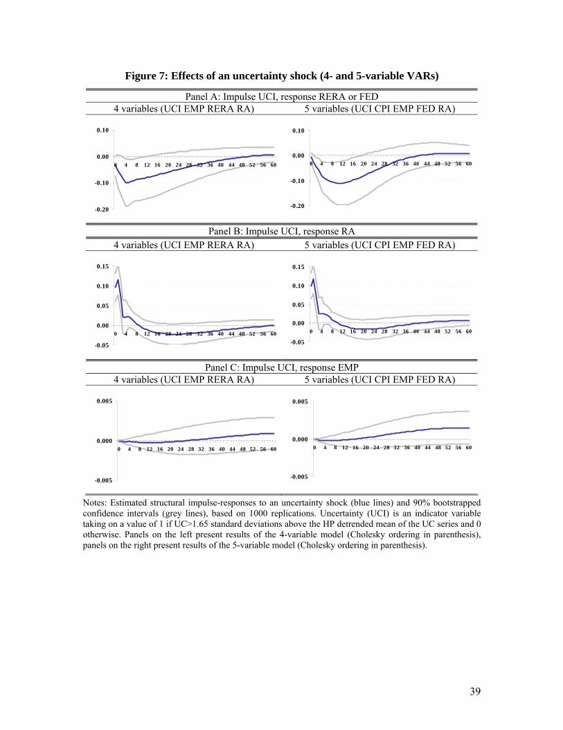
Figure 7: Effects of an uncertainty shock (4- and 5-variable VARs)

Panel A: Impulse UCI, response RERA or FED 4 variables (UCI EMP RERA RA) 5 variables (UCI CPI EMP FED RA)

-0.20

-0.10

0.00

0.10

0 4 8 12 16 20 24 28 32 36 40 44 48 52 56 60

-0.20

-0.10

0.00

0.10

0 4 8 12 16 20 24 28 32 36 40 44 48 52 56 60

Panel B: Impulse UCI, response RA 4 variables (UCI EMP RERA RA) 5 variables (UCI CPI EMP FED RA)

-0.05

0.00

0.05

0.10

0.15

0 4 8 12 16 20 24 28 32 36 40 44 48 52 56 60

-0.05

0.00

0.05

0.10

0.15

0 4 8 12 16 20 24 28 32 36 40 44 48 52 56 60

Panel C: Impulse UCI, response EMP 4 variables (UCI EMP RERA RA) 5 variables (UCI CPI EMP FED RA)

-0.005

0.000

0.005

0 4 8 12 16 20 24 28 32 36 40 44 48 52 56 60

-0.005

0.000

0.005

0 4 8 12 16 20 24 28 32 36 40 44 48 52 56 60

Notes: Estimated structural impulse-responses to an uncertainty shock (blue lines) and 90% bootstrapped confidence intervals (grey lines), based on 1000 replications. Uncertainty (UCI) is an indicator variable taking on a value of 1 if UC>1.65 standard deviations above the HP detrended mean of the UC series and 0 otherwise. Panels on the left present results of the 4-variable model (Cholesky ordering in parenthesis), panels on the right present results of the 5-variable model (Cholesky ordering in parenthesis).

39

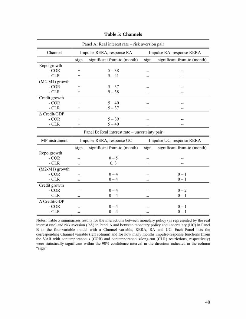
40

Table 5: Channels

Panel A: Real interest rate – risk aversion pair

Channel Impulse RERA, response RA Impulse RA, response RERA

sign significant from-to (month) sign significant from-to (month) Repo growth

- COR - CLR

+ +

5 – 38 5 – 41

-- --

(M2-M1) growth - COR - CLR

+ +

5 – 37 9 – 38

-- --

Credit growth - COR - CLR

+ +

5 – 40 5 – 37

-- --

Δ Credit/GDP - COR - CLR

+ +

5 – 39 5 – 40

-- --

Panel B: Real interest rate – uncertainty pair

MP instrument Impulse RERA, response UC Impulse UC, response RERA

sign significant from-to (month) sign significant from-to (month) Repo growth

- COR - CLR

0 – 5 0, 3

-- --

(M2-M1) growth - COR - CLR

0 – 4 0 – 4

0 – 1 0 – 1

Credit growth - COR - CLR

0 – 4 0 – 4

0 – 2 0 – 1

Δ Credit/GDP - COR - CLR

0 – 4 0 – 4

0 – 1 0 – 1

Notes: Table 5 summarizes results for the interactions between monetary policy (as represented by the real interest rate) and risk aversion (RA) in Panel A and between monetary policy and uncertainty (UC) in Panel B in the four-variable model with a Channel variable, RERA, RA and UC. Each Panel lists the corresponding Channel variable (left column) and for how many months impulse-response functions (from the VAR with contemporaneous (COR) and contemporaneous/long-run (CLR) restrictions, respectively) were statistically significant within the 90% confidence interval in the direction indicated in the column “sign”.