GCV for Tikhonov regularization by partial SVDreichel/publications/gcv.pdfGCV for Tikhonov...

BIT manuscript No.(will be inserted by the editor)

GCV for Tikhonov regularization by partial SVD

Caterina Fenu · Lothar Reichel ·Giuseppe Rodriguez · Hassane Sadok

Received: date / Accepted: date

Abstract Tikhonov regularization is commonly used for the solution of linear dis-

crete ill-posed problems with error-contaminated data. A regularization parameter

that determines the quality of the computed solution has to be chosen. One of the

most popular approaches to choosing this parameter is to minimize the Generalized

Cross Validation (GCV) function. The minimum can be determined quite inexpen-

sively when the matrix A that defines the linear discrete ill-posed problem is small

enough to rapidly compute its singular value decomposition (SVD). We are inter-

ested in the solution of linear discrete ill-posed problems with a matrix A that is too

large to make the computation of its complete SVD feasible, and show how upper

and lower bounds for the numerator and denominator of the GCV function can be

determined fairly inexpensively for large matrices A by computing only a few of the

largest singular values and associated singular vectors of A. These bounds are used

to determine a suitable value of the regularization parameter. Computed examples

illustrate the performance of the proposed method.

Keywords Generalized cross validation · Tikhonov regularization · partial singular

value decomposition

Mathematics Subject Classification (2000) 65F22 · 65F20 · 65R32

C. Fenu

Dipartimento di Informatica, Universita di Pisa, Largo Pontecorvo 3, 56127 Pisa, Italy.

E-mail: [email protected]

L. Reichel

Department of Mathematical Sciences, Kent State University, Kent, OH 44242, USA.


G. Rodriguez

Dipartimento di Matematica e Informatica, Universita di Cagliari, viale Merello 92, 09123 Cagliari, Italy.


H. Sadok

Laboratoire de Mathematiques Pures et Appliquees, Universite du Littoral, Centre Universtaire de la Mi-

Voix, Batiment H. Poincarre, 50 Rue F. Buisson, BP 699, 62228 Calais cedex, France.


2 Caterina Fenu et al.

1 Introduction

We are interested in the solution of large-scale least-squares problems

minx∈Rn

‖Ax−b‖, (1.1)

where A∈Rm×n is a large matrix whose singular values decay gradually to zero with-

out a significant gap. In particular, the Moore–Penrose pseudoinverse of A, denoted

by A†, is of very large norm. Least-squares problems of this kind often are referred

to as linear discrete ill-posed problems. The data vector b ∈ Rm is assumed to stem

from measurements and be contaminated by a measurement error e∈Rm of unknown

size. We will assume that m ≥ n for notational simplicity, but the method discussed

also can be applied when m < n after appropriate modifications.

Let b denote the unknown error-free vector associated with b. Thus, b = b+ e.

We would like to compute x := A†b. The solution

A†b = x+A†e

of (1.1) generally is not a meaningful approximation of x, because typically ‖A†e‖≫‖x‖. Here and throughout this paper ‖ · ‖ denotes the Euclidean vector norm or the

spectral matrix norm. To compute a useful approximation of x, one often applies

Tikhonov regularization, i.e., one replaces the problem (1.1) by the penalized least-

squares problem

minx∈Rn

{‖Ax−b‖2 +µ‖x‖2

}, (1.2)

where µ > 0 is a regularization parameter. It is the purpose of the regularization term

µ‖x‖2 to damp the propagated error in the computed approximation of x. However,

it can be difficult to determine a suitable value of µ when no accurate bound for

the norm of the error e in b is known. A too small value of µ gives a solution that

is severely contaminated by the propagated error, and a too large value yields an

unnecessarily poor approximation of x; see, e.g., [13,15,20,26] for discussions on

Tikhonov regularization and the choice of µ . For future reference, we note that the

Tikhonov minimization problem (1.2) for any µ > 0 has the unique solution

xµ = (AT A+µI)−1AT b, (1.3)

where the superscript T denotes transposition and I is the identity matrix.

One of the most popular methods for determining a suitable value of µ when

no accurate bound for ‖e‖ is available is the Generalized Cross Validation (GCV)

method; see [10,16,20,26,28]. This method chooses a regularization parameter that

minimizes the GCV function

V (µ) :=‖Axµ −b‖2

(trace(I −A(µ)))2, (1.4)

where the influence matrix is defined by

A(µ) := A(AT A+µI)−1AT (1.5)

GCV for Tikhonov regularization by partial SVD 3

and xµ is the Tikhonov solution (1.3). Thus, A(µ)b = Axµ . Let µ∗ > 0 minimize

(1.4). Numerical experiments indicate that the minimum of (1.4) generally is unique;

in case of nonunicity, we let µ∗ be the largest minimum. The GCV method prescribes

that xµ∗ be used as an approximate solution of (1.1). We remark that determining µ∗

generally requires that the GCV function be evaluated for several µ-values.

When the matrix A is of small to moderate size, the evaluation of the singular

value decomposition (SVD) of A is feasible. It is inexpensive to evaluate V (µ) for

different µ-values when the SVD of A is available. However, when A is large, the

computation of its SVD is too expensive to be attractive. We describe how upper and

lower bounds for the GCV function can be determined from a partial SVD that is

made up of a few, say k, of the largest singular values of A and associated singular

vectors. Computed examples in [29] illustrate that the computation of the 1 ≤ k ≪ n

largest singular values and associated singular vectors of A is fairly inexpensive when

A is the matrix of a linear discrete ill-posed problem; several examples taken from

[21] show that the number of matrix-vector product evaluations with A and AT re-

quired is only a small multiple of k. These computations apply an implicitly restarted

Golub–Kahan bidiagonalization method; see, e.g., [3,4,25] for discussions on implic-

itly restarted bidiagonalization methods. Also other approaches to determining a few

singular values and vectors of a large matrix, such as those described in [22,23,31]

can be used. We remark that the evaluation of the matrix-vector products constitutes

the dominating computational work.

The availability of a partial SVD of A makes it possible to compute an approxima-

tion of the Tikhonov solution (1.3), and allows the determination of upper and lower

bounds for the numerator and denominator of the GCV function. These bounds yield

useful bounds for the GCV function (1.4). We will use the upper bound of the GCV

function, rather than the function itself, to determine a suitable value of the regular-

ization parameter.

Several other methods for bounding or estimating the GCV function have been

described in the literature. An approach to compute upper and lower bounds for V (µ)based on the connection between standard and global Golub–Kahan bidiagonaliza-

tion with Gauss quadrature is discussed in [14]. The method of the present paper

is faster when the singular values of A decay to zero quickly. Golub and von Matt

[19] estimate the denominator of (1.4) with the aid of Hutchinson’s trace estimator

[24] and bound the numerator by using the connection between Golub–Kahan bidi-

agonalization and Gauss quadrature; see also Bai et al. [5] for related methods. The

computations described in [19] can be carried out efficiently for large-scale prob-

lems; however, Hutchinson’s trace estimator is not reliable; see [14] for illustrations.

Elden [12] shows that it suffices to reduce A to bidiagonal form, instead of comput-

ing the SVD. Randomized algorithms for estimating the trace of a large matrix are

surveyed by Avron and Toledo [1]. These algorithms typically require a large number

of matrix-vector product evaluations to yield estimates of moderate to high accuracy.

Novati and Russo [28] describe how carrying out a few steps of the Arnoldi process

applied to A with initial vector b can give estimates of the GCV function (1.4). Ap-

proaches based on extrapolation and probing for approximating the trace of a large

symmetric implicitly defined matrix are presented by Brezinski et al. [8,9], and Tang

and Saad [32]. We remark that the method of the present paper may be attractive


to use for the applications discussed in [8,9,32] if the matrix whose trace is to be

determined stems from a discrete ill-posed problem.

In some applications of Tikhonov regularization, the minimization problem (1.2)

is replaced by a problem of the form

minx∈Rn

{‖Ax−b‖2 +µ‖Lx‖2} (1.6)

with a matrix L ∈ Rp×n different from the identity. Common choices of the matrix L

include scaled discretizations of differential operators such as the tridiagonal matrix

L =

−1 2 −1 O1 2 −1

. . .. . .

. . .

O −1 2 −1

∈ R

(n−2)×n.

The choice of an orthogonal projection L ∈ Rn×n is discussed in [27]. Bjorck [6] and

Elden [11] describe how the minimization problem (1.6) can be brought into the form

(1.2). We will therefore only consider Tikhonov regularization problems of the form

(1.2) in the present paper.

This paper is organized as follows. Section 2 discusses how bounds for the de-

nominator of the GCV function can be computed by using a partial SVD of the matrix

A, and the computation of bounds for the numerator is described in Section 3. The

evaluation of bounds for the GCV function is considered in Section 4, where also an

algorithm is presented. The partial SVD of A allows the computation of an approx-

imate solution of the Tikhonov minimization problem (1.2). Computed examples in

Section 5 illustrate the performance of the proposed method and Section 6 contains

concluding remarks.

2 Bounding the denominator of the GCV function

This section describes how upper and lower bounds for the denominator of the GCV

function (1.4) can be computed with the aid of a partial SVD of the matrix A. Intro-

duce the (full) SVD of A,

A =UΣV T , (2.1)

where U = [u1,u2, . . . ,um] ∈ Rm×m and V = [v1,v2, . . . ,vn] ∈ R

n×n are orthogonal

matrices, and Σ = diag[σ1,σ2, . . . ,σn] ∈ Rm×n is a (possibly rectangular) diagonal

matrix with nonnegative diagonal entries. The diagonal entries are the singular values

of A; they are ordered according to

σ1 ≥ σ2 ≥ ·· · ≥ σn ≥ 0.

The columns u j of U are commonly referred to as the left singular vectors of A, and

the columns v j of V as the right singular vectors. We refer to the singular triplets

{σ j,u j,v j}kj=1 associated with the k largest singular values as the k largest singu-

lar triplets of A. The bounds of the following proposition only require the k largest

singular values to be known.


Proposition 2.1 Let the matrix A ∈ Rm×n have the singular value decomposition

(2.1) and let A(µ) denote the influence matrix (1.5). Then for µ > 0 and 1 ≤ k ≤ n,

we have

wk − sk ≤ trace(I −A(µ))≤ wk, (2.2)

where

wk = m−k

∑j=1

σ2j

σ2j +µ

, sk = (n− k)σ2

k

σ2k +µ

.

Proof Substituting (2.1) into (1.5) yields

A(µ) =UΣ(Σ T Σ +µI)−1Σ TUT .

Therefore,

trace(I −A(µ)) = m−n

∑j=1

σ2j

σ2j +µ

. (2.3)

This shows the right-hand side inequality of (2.2). To show the left-hand side inequal-

ity, we introduce the function

f (t) =t

t +µ. (2.4)

It is strictly increasing for t ≥ 0 (and fixed µ > 0). Therefore

trace(A(µ))≤k

∑j=1

σ2j

σ2j +µ

+(n− k)σ2

k

σ2k +µ

. (2.5)

This completes the proof.

The bound (2.5) can be sharpened by replacing σk by σk+1 in the trailing term,

and this would give a sharper lower bound than (2.2). We are interested in the bounds

(2.2) because they can be evaluated when the first k singular values of A are known.

The accuracy of the approximation induced by the bounds (2.2) is proportional to

the ratio σ2k /(σ

2k + µ). The following proposition investigates how this accuracy is

influenced by the presence of errors in the singular values.

Proposition 2.2 Let the computed singular values σ j be perturbed by errors, such

that |σ j −σ j| ≤ τ , j = 1,2, . . . ,n. Let sk be the difference between the corresponding

perturbed upper and lower bounds (2.2). Then

sk ≤ sk +(n− k)τ

σ2k +µ

. (2.6)

Proof We can assume that the perturbed singular values σ j are the exact singular

values of a perturbed matrix A + E, with ‖E‖ ≤ τ . The stability theorem for the

singular values [7] states that

|σ j −σ j| ≤ ‖E‖,which implies

σ2k

σ2k +µ

≤ σ2k +‖E‖2

σ2k +‖E‖2 +µ

≤ σ2k

σ2k +µ

+‖E‖2

σ2k +µ

.

Inequality (2.6) follows immediately.


The above result shows that, when the singular values are perturbed, the accuracy

of the bounds changes significantly only if the singular value σk, corresponding to the

truncation parameter k, is comparable, or smaller, than the maximum absolute error

τ in the singular values. This situation does not take place when the singular values

decrease to zero quickly with increasing index number and there is a fairly large error

e in the data b.

Proposition 2.1 assumes that the k largest singular values of A are available. How-

ever, due to the fact that any algorithm used for their computation is terminated after

finitely many steps and because of round-off errors introduced during the calcula-

tions, only approximations of these singular values are known. The following result

complements Proposition 2.2 and is concerned with the sensitivity of the bounds of

Proposition 2.1 to errors in the singular values.

Corollary 2.1 Assume that not the singular values σ j, 1≤ j ≤ k, of A, but only lower

and upper bounds σ−j and σ+

j for these singular values are known. Let these bounds

be such that

σ−j ≤ σ j ≤ σ+

j , 1 ≤ j ≤ k. (2.7)

Then, for µ > 0 and 1 ≤ k ≤ n, we have

m−k

∑j=1

(σ+j )

2

(σ+j )

2 +µ− (n− k)

(σ+k )2

(σ+k )2 +µ

≤ trace(I −A(µ))≤ m−k

∑j=1

(σ−j )

2

(σ−j )

2 +µ.

Proof The inequalities can be shown similarly as those of Proposition 2.1. For in-

stance, using (2.3) and the fact that the function (2.4) is increasing, we obtain

trace(I −A(µ))≤ m−n

∑j=1

(σ−j )

2

(σ−j )

2 +µ.

The desired upper bound for trace(I −A(µ)) now follows. Similarly,

trace(I −A(µ))≥ m−n

∑j=1

(σ+j )

2

(σ+j )

2 +µ,

which yields the lower bound for trace(I −A(µ)).

In applications of the bounds of the present paper, generally, all one knows about

the matrix A are its k ≪ n largest singular triplets. It is therefore natural to replace A

by its best rank-k approximation

Ak =UkΣkVTk , (2.8)

which is defined by these triplets. Thus, Uk ∈ Rm×k is made up of the k first columns

of the matrix U in (2.1), Vk ∈ Rn×k is made up of the k first columns of V , and

Σk ∈ Rk×k is the leading principal submatrix of Σ of order k. The analogues of the

bounds of Proposition 2.1 and Corollary 2.1 for Ak read as follows. Their proofs are

similar to the proofs already shown and therefore are omitted.


Proposition 2.3 Let the matrix Ak ∈ Rm×n be defined by (2.8) and let Ak(µ) denote

the associated influence matrix (obtained by replacing A by Ak in (1.5)). Then for

µ > 0, we have

trace(I −Ak(µ)) = m−k

∑j=1

σ2j

σ2j +µ

.

Assume that the singular values σ j of A are not known, but lower and upper

bounds σ−j and σ+

j that satisfy (2.7) are available. Then for µ > 0, we have

m−k

∑j=1

(σ+j )

2

(σ+j )

2 +µ≤ trace(I −Ak(µ))≤ m−

k

∑j=1

(σ−j )

2

(σ−j )

2 +µ.

It is interesting to observe that the upper bound for the trace is the same as in

Corollary 2.1.

Remark 2.1 When the block Lanczos bidiagonalization algorithm (also known as the

block Golub–Kahan bidiagonalization algorithm) [17] is applied to the computation

of the k largest singular triplets, the following bounds for the singular values hold,

σ−j = θ j and σ+

j = θ j +ε2

j

σ j

≤ θ j +ε2

j

θ j

,

where θ j is the jth singular value of the bidiagonal matrix computed at the sth step

of the algorithm; see [17, Theorem 3.2]. The parameter ε2j , which can be expressed

in terms of the reciprocal of the square of a Chebyshev polynomial of the first kind

evaluated outside the interval [−1,1], usually is very small for the largest singular

values. We therefore can expect the largest singular values of A to be computed with

high accuracy; see [17, Example 3.2] and the end of Section 5 for illustrations.

3 Bounding the numerator of the GCV function

Let xµ be given by (1.3). This section derives bounds for ‖Axµ −b‖2 whose evalua-

tion requires the first k singular values σ1,σ2, . . . ,σk of A and associated left singular

vectors u1,u2, . . . ,uk. Substituting the SVD (2.1) of A into ‖Axµ −b‖2 and letting

b = [b1, b2, . . . , bm]T :=UT b, (3.1)

where the matrix U is from the SVD of A, yields

‖Axµ −b‖2 = µ2bT (ΣΣ T +µI)−2b =n

∑j=1

µ2b2j

(σ2j +µ)2

+m

∑j=n+1

b2j . (3.2)

Proposition 3.1 Let µ > 0 and let xµ be the solution (1.3) of the Tikhonov minimiza-

tion problem (1.2). Then the following upper bound holds

‖Axµ −b‖2 ≤ uk :=k

∑j=1

µ2b2j

(σ2j +µ)2

+ ck, (3.3)


where

ck :=m

∑j=k+1

b2j = ‖b‖2 −

k

∑j=1

b2j , (3.4)

can be evaluated when the first k singular values σ1,σ2, . . . ,σk of A and the associ-

ated left singular vectors u1,u2, . . . ,uk are available.

Proof The function

g(t) = (t +µ)−2, µ > 0, t ≥ 0, (3.5)

is strictly decreasing for 0 ≤ t < ∞ and fixed µ > 0. In particular, its maximum is

g(0) = 1/µ2 and limt→∞ g(t) = 0. It follows that

0 ≤µ2b2

j

(σ2j +µ)2

≤ b2j .

Substituting this inequality into (3.2) gives (3.3). The relation (3.4) is a consequence

of ‖b‖= ‖b‖.

We remark that when k in (3.3) is large enough so that σ2k+1 is small, the bound

is quite sharp. The following lower bound generally is less sharp.

Proposition 3.2 Let µ > 0 and let xµ be the solution (1.3) of the Tikhonov minimiza-

tion problem (1.2). Then

‖Axµ −b‖2 ≥ uk − rk, (3.6)

where

rk =σ2

k (σ2k +2µ)

(σ2k +µ)2

ck,

and uk and ck are defined by (3.3) and (3.4), respectively. The lower bound (3.6) can

be evaluated by using only the first k singular triplets of A.

Proof It follows from the properties of the function (3.5) that the right-hand side of

(3.2) can be bounded below by

‖Axµ −b‖2 ≥k

∑j=1

µ2b2j

(σ2j +µ)2

+µ2

(σ2k +µ)2

n

∑j=k+1

b2j +

m

∑j=n+1

b2j . (3.7)

Using the fact that µ2/(σ2k +µ)2 ≤ 1, we obtain the lower bound (3.6) for the right-

hand side of (3.7).

A looser but simpler bound can be obtained as follows.

Corollary 3.1 Under the assumptions of the preceding proposition, it holds

‖Axµ −b‖2 ≥ uk −2σ2

k

σ2k +µ

ck.


Proof The result follows from

σ2k (σ

2k +2µ)

(σ2k +µ)2

=σ2

k

σ2k +µ

(1+

µ

σ2k +µ

)≤ 2σ2

k

(σ2k +µ)

.

Other bounds can be derived by relating k to the size of µ . The following propo-

sition furnishes an example.

Proposition 3.3 We use the notation of Proposition 3.2 and let m = n. Assume that k

is chosen so that σ2k+1 ≤ µ . Then it holds

1

4

n

∑j=k+1

b2j ≤ ‖Axµ −b‖2 −

k

∑j=1

µ2b2j

(σ2j +µ)2

≤n

∑j=k+1

b2j . (3.8)

Proof The right-hand side inequality follows from (3.3). To show the left-hand side

inequality, we note that σ2j ≤ µ implies

µ2b2j

(σ2j +µ)2

≥µ2b2

j

(µ +µ)2=

1

4b2

j .

Therefore,n

∑j=k+1

µ2b2j

(σ2j +µ)2

≥ 1

4

n

∑j=k+1

b2j .

The left-hand side inequality of (3.8) now follows from (3.2).

When the singular values are perturbed by errors, the following result can be

shown similarly as Proposition 2.2.

Proposition 3.4 Let the computed singular values σ j be perturbed by errors, such

that |σ j −σ j| ≤ τ , j = 1, . . . ,n. Let rk be the difference between the corresponding

perturbed upper and lower bounds given in Proposition 3.1 and Corollary 3.1. Then

rk ≤2σ2

k

σ2k +µ

ck +2τ

σ2k +µ

ck.

We conclude this section by discussing some inequalities that are analogous to

those of Propositions 3.1 and 3.2, and that can be applied when only approximations

of the k first singular values of A and of the k first entries of the vector (3.1) are

known. It is natural that bounds in terms of computed quantities only should involve

these quantities. This suggests that the matrix Ak be used in the bounds, and that only

part of the residual error be considered.

Corollary 3.2 Let, for 1 ≤ j ≤ k, the singular value bounds σ−j and σ+

j satisfy (2.7),

and let |b j|+ and |b j|− be available upper and lower bounds for |b j|. Then

‖Akxk,µ −UkUTk b‖2 ≤

k

∑j=1

µ2(|b j|+)2

((σ−j )

2 +µ)2, (3.9)


where Uk is defined in (2.8) and

xk,µ =VkΣk(Σ2k +µI)−1ΣkU

Tk b.

Further,

‖Akxk,µ −UkUTk b‖2 ≥

k

∑j=1

µ2(|b j|−)2

((σ+j )

2 +µ)2, (3.10)

Proof The upper bound (3.9) follows from (2.8) and the form of solution xk,µ . The

derivation of the bound assumes that the columns of the matrices Uk and Vk are or-

thonormal, but they are not required to be exact left and right singular vectors, respec-

tively. The orthogonality requirement can be satisfied by reorthogonalization, which

generally is used in the computation of partial singular value decompositions (2.8);

see, e.g., [3,4]. When the orthogonal projector UkUTk is ignored in (3.9), the term

‖(I −UkUTk )b‖2 has to be added to the right-hand side. This term is independent of

µ and therefore does not affect the location of the minimum (or minima) of the GCV

function.

The lower bound (3.10) follows similarly. This bound is simpler than the corre-

sponding bound (3.6) of Proposition 3.2.

As explained in the following section, the difference between available upper and

lower bounds for the GCV function is used to determine how many singular triplets

to compute. The location of the (a) minimum of the upper bound determines the value

of the regularization parameter.

4 Bounding the GCV function

From the upper and lower bounds for the denominator and numerator of the GCV

function derived in Sections 2 and 3, it is immediate to obtain bounds for the ratio.

Let uk and ℓk := uk − rk denote the upper and lower bounds, respectively, of the

numerator of the GCV function of Propositions 3.1 and 3.2. Thus, we have

ℓk ≤ ‖Axµ −b‖2 ≤ uk.

Moreover, let

vk ≤ trace(I −A(µ))≤ wk,

where wk and vk := wk − sk are the bounds of Proposition 2.1. Then,

Lk ≤ V (µ)≤ Uk, (4.1)

with Lk = ℓk/w2k and Uk = uk/v2

k . Note that these bounds depend on µ > 0.

We remark that it is straightforward to use the bounds for the approximations of

singular triplets described in Sections 2 and 3 instead of the bounds of Propositions

3.1 and 3.2. Therefore, we will only discuss the use of the latter bounds in this section.

In order to understand the behavior of the bounds (4.1), we consider the approxi-

mation errors rk and sk induced by the bounds for the numerator and the denominator;


see also Corollary 3.1. Both the errors depend on the ratio σ2k /(σ

2k +µ). For a fixed

tolerance τ , we have that

σ2k

σ2k +µ

< τ implies σ2k <

τ

1− τµ .

Therefore, the bounds will be sharp for µ in some interval [µ0,µ f ] only for k such

that σk ≪ µ0. The interval will expand towards the left when k increases. This effect

is observed in Figure 5.1 and 5.2 of Section 5.

In real-world applications, the error e in the data b is generally quite large, say

0.5% and larger. The minimum of the GCV function then is achieved at a not very

small value of µ . If the singular values decay rapidly, as is the case for many discrete

ill-posed problems, then we expect to obtain reliable bounds for V (λ ) in a neigh-

borhood of the minimum already for a fairly small value of k. This is illustrated in

Section 5.

Let the singular triplets {σ j,u j,v j}kj=1 be available. Then we evaluate the up-

per and lower bounds Uk and Lk, respectively, for a discrete set of values of the

regularization parameter µ . We store the elements of this set in the vector λ =[λ1,λ2, . . . ,λp]

T . The remainder of this section provides a discussion of our scheme

for determining an approximation of the minimum of the GCV function. Details are

described by Algorithm 1 below. In the algorithm, vectors are in bold, MATLAB no-

tation is used for vector operations, and the square of a vector means squaring its

components. The expressions in square brackets at line 19 produce the logical results

true or false. The variable S, which is initialized at line 5 and updated at line 13, con-

tains successive values of the quantity (3.4). Due to propagated round-off errors, this

quantity may achieve a small negative value when many iterations are carried out.

This situation is remedied at line 14, where the variable S is set to zero if it is found

to be of magnitude smaller than a tiny positive constant eps.

We have observed in numerous numerical examples that the minimum of the

upper bound quickly converges to the minimum of V (µ), i.e., the minimum of the

upper bound yields a quite accurate location of the minimum of the GCV function

already for a fairly small number, k, of singular triplets. However, when µ > 0 is

tiny, the lower bound may be much smaller than the global minimum of the GCV

function; see Figures 5.1 and 5.2 for illustrations. Algorithm 1 therefore estimates

the location of the minimum of the GCV function from the upper bound; the lower

bound is primarily used to determine whether the number of available singular triplets

is large enough. Thus, at each step ℓ we identify the minimum µℓ of the upper bound

for V (µ), and we stop the iteration if either the bounds converge near the minimum,

i.e., if for a given tolerance τ > 0,

Uℓ−Lℓ

Uℓ+Lℓ≤ τ ,

or if the minimum does not change much, that is, if

|µℓ−µℓ−1| ≈ |µℓ−1 −µℓ−2|. (4.2)


To avoid that the iterations be terminated while the convergence is still erratic, we

apply the condition (4.2) only after the difference |µℓ − µℓ−1| has decreased for at

least two subsequent iterations; see lines 19–21 of Algorithm 1.

The algorithm is initially applied to a vector λ with 12 components λk that are

logarithmically spaced in [10−10,10]. In case the minimum is at one end point, we

shift the interval and repeat the computation. If the minimum is at an internal point

λk, we apply the algorithm to 100 values in [λk−1,λk+1].

Algorithm 1 Bounding the GCV function by partial SVD.

1: Input: Singular triplets (σ j,u j,v j) of A, u j ∈ Rm, v j ∈ R

n, j = 1 . . . ,k;

2: noisy right hand side b; vector of Tikhonov parameters λ ∈ Rp;

3: tolerances τ and η .

4: s = σ21 , β = (uT

1 b)2

5: t = λ 2./(s+λ )2, w = β t, S = ‖b‖2 −β6: U1 = w+S, L1 = w+St

7: t = s./(s+λ ), U2 = m− t, L2 = U2 − (n−1)t8: U = U1/L2

2, L = L1/U22

9: ωℓ = min(U ), µ = λℓ

10: j = 1, ε = 0, c = 0, flag = true

11: while flag

12: j = j+1, µ = µ , ε = ε , s = σ2j , β = (uT

j b)2

13: t = λ 2./(s+λ )2, w = w+β t, S = S−β14: if |S|< eps then S = 0 end

15: U1 = w+S, L1 = w+St

16: t = s./(s+λ ), U2 = U2 − t, L2 = U2 − (n− j)t17: U = U1/L2

2, L = L1/U22

18: ωℓ = min(U ), µ = λℓ, ε = |µ − µ|19: flag = [( j < k) and ((Uℓ−Lℓ)/(Uℓ+Lℓ)> τ)]20: if (ε < ε) then c = c+1 else c = 0 end

21: if (c ≥ 2) then flag = [flag and (|ε − ε|> η)] end

22: end while

23: Output: Tikhonov parameter µ , lower and upper bounds Lℓ, Uℓ for V (µ).

Typically, the number of singular triplets of the matrix A in (1.1) required to sat-

isfy the stopping criterion of Algorithm 1 is not known before application of the

algorithm. Therefore, when applying the algorithm to large-scale problems, it has to

be combined with a suitable procedure for computing the required singular triplets.

To this end, we adopted the same computational scheme that was applied in [2] in the

context of complex network analysis. We first compute the p largest singular triplets

{σ j,u j,v j}pj=1 of A by the augmented implicitly restarted Golub–Kahan bidiagonal-

ization method described in [3]. If more singular triplets are required to satisfy the

stopping criterion of Algorithm 1, we use a slight modification of the MATLAB func-

tion from [3], which allows the computation to be restarted, to determine a new batch

of triplets {σ j,u j,v j}2pj=p+1. We repeat this process as many times as necessary to

satisfy the stopping criterion.

We found in numerous numerical experiments that when k is the index that sat-

isfies the stopping criterion of Algorithm 1, the difference ‖xµ − xk,µ‖ between the

Tikhonov solution xµ and the corresponding truncated SVD approximation xk,µ is


10 -24 10 -20 10 -16 10 -12 10 -8 10 -4 10 0

10 -20

10 -15

10 -10

10 -5k=1

k=3

k=5

k=7

Fig. 5.1 Upper and lower bounds for the Wing test problem of size 100× 100 with noise level 10−6, as

functions of µ . The thick line represents the GCV function V (µ), while the thin lines are the computed

bounds Uk and Lk, k = 1,3,5,7.

negligible compared with the error in the Tikhonov solution ‖x−xµ‖, where x = A†b

denotes the desired solution of the error-free least-squares problem associated with

(1.1).

5 Computed examples

We implemented Algorithm 1 in MATLAB to illustrate the effectiveness of the bounds

computed by the algorithm for estimating the minimum of the GCV function and in

this manner determining a suitable value of the parameter for Tikhonov regulariza-

tion. All computations were carried out with about 16 significant decimal digits on

an Intel Core i7/860 computer with 8Gb RAM running Linux. The algorithm was

applied to the discrete ill-posed problems listed in Table 5.1, some of which are

from Hansen’s Regularization Tools [21] and some from the MATLAB gallery

function. While the problems from [21] come with a model solution x, the ones

from the gallery function do not. We associated with the latter the exact solution

xBaart of the Baart test problem from Regularization Tools and determined the ex-

act right-hand side according to b = AxBaart. For all test problems, we generate an

error-contaminated right-hand side b according to

b = b+δ‖b‖√

mn,

where n ∈ Rm is a random white noise vector, with zero mean and variance one, and

δ is the noise level.


We first consider some small-scale examples, for which we can compute the (full)

singular value decomposition by the svd function of MATLAB. Figure 5.1 displays

the bounds obtained from (4.1), as functions of µ , for the linear discrete ill-posed

problem (1.1) Wing from [21] with A ∈R100×100 and the small noise level δ = 10−6.

Algorithm 1 carries out 7 iterations and correctly determines the location of the mini-

mum of V (µ), displayed by a red circle in the graph. The upper and lower bounds Uk

and Lk approximate the GCV function V (µ) well over larger µ-intervals the larger

k is.

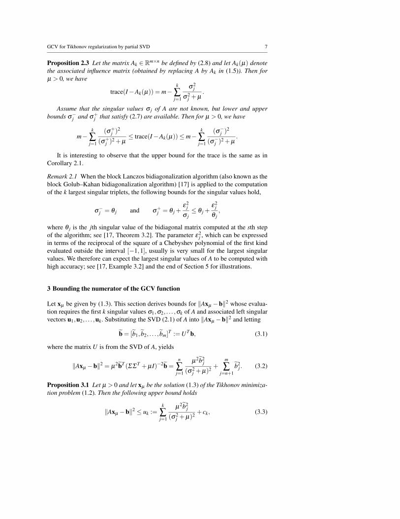
Figure 5.2 is analogous to Figure 5.1 and shows the upper and lower bounds

from (4.1) for a linear discrete ill-posed problem (1.1) with a rectangular matrix A.

Specifically, A is defined by the first 40 columns of a Shaw matrix of order 60. The

latter is generated by software in [21]. The noise level in this example is δ = 10−2;

this noise level is representative for many linear discrete ill-posed problems that have

to be solved in science and engineering. Algorithm 1 carried out 13 steps for the

present example before satisfying the stopping criterion. The computed minimum

gives a value of the the regularization parameter that is very close to the best possible.

10 -20 10 -16 10 -12 10 -8 10 -4 10 0

10 -6

10 -5

10 -4

10 -3

10 -2

10 -1

k=1

k=3

k=5

k=7k=9k=11k=13

Fig. 5.2 Upper and lower bounds for the Shaw test problem of size 60× 40 with noise level 10−2, as

functions of µ . The thick line represents the GCV function V (µ), while the thin lines are the computed

bounds Uk and Lk, k = 1,3, . . . ,13.

To investigate the accuracy of the bounds when determining a suitable value of

the Tikhonov regularization parameter, we constructed for each test problem a set

of 60 least squares problems, both square (200× 200) and rectangular (400× 200)

ones, by letting the noise level take on the values 10−4, 10−3, and 10−2. For each

problem and noise level, we generated 10 random noise vectors e and determined

for each one of the 60 numerical examples so defined the regularization parameter µby Algorithm 1 as well as the regularization parameter µbest that gives the smallest


relative error in the Euclidean norm, i.e.,

Eopt :=‖xµbest

− x‖‖x‖ = min

µ>0

‖xµ − x‖‖x‖ , (5.1)

where x is the desired solution of the error-free problem associated with (1.1). Let

Fκ denote the number of experiments for which the computed regularized solution

xµ with µ determined by Algorithm 1 yields a relative error larger than κ times the

optimal error, that is, the number of times the following inequality holds

‖xµ − x‖‖x‖ > κ

‖xµbest− x‖

‖x‖ . (5.2)

Table 5.1 shows the results obtained for solutions determined by Algorithm 1, de-

noted by gcvpsvd, and compares them to results produced by the gcv function from

[21]. We report, for each group of 60 test problems, the average Eopt of the optimal

error (5.1) and the values of Fκ , κ = 5,10, for the two methods. In the table, Eκ de-

notes the average of the relative errors that do not exceed the limit imposed by (5.2).

The results show Algorithm 1 to perform essentially as well as the standard approach

for minimizing V (µ) as implemented by the gcv function from [21]. The slightly

better performance of Algorithm 1 is probably due to the fact that the GCV function

for some problems is extremely flat near the minimum, and this may lead to inaccu-

racy in the computation of the minimum. The table indicates that the minimization

of the upper bound of the GCV function, as implemented by Algorithm 1, performs

somewhat better than the minimization of the GCV function as implemented by the

gcv function from [21].

Table 5.1 Comparison of two GCV minimization algorithms across the solution of 10 test problems, each

composed by 60 numerical examples obtained by varying the size of the problem, the noise level, and by

considering different realizations of the noise; see text.

gcv gcvpsvd

matrix Eopt F5 E5 F10 E10 F5 E5 F10 E10

Baart 1.8e-01 14 5.9e-01 14 5.9e-01 4 5.4e-01 4 5.4e-01

Deriv2(2) 2.6e-01 1 5.6e-01 0 1.8e+00 0 2.7e-01 0 2.7e-01

Foxgood 5.7e-02 12 1.2e-01 3 4.5e-01 9 1.2e-01 2 4.4e-01

Gravity 3.7e-02 16 4.7e-02 13 1.9e-01 14 4.7e-02 9 2.4e-01

Heat(1) 1.3e-01 0 3.7e-01 0 3.7e-01 0 1.7e-01 0 1.7e-01

Hilbert 4.5e-01 4 6.4e-01 4 6.4e-01 2 6.4e-01 0 6.4e-01

Lotkin 4.6e-01 4 1.2e+00 2 1.2e+00 3 7.1e-01 1 7.1e-01

Phillips 3.7e-02 4 1.3e-01 2 1.3e-01 0 8.4e-02 0 8.4e-02

Shaw 1.3e-01 18 1.2e-01 14 3.5e-01 6 1.9e-01 5 1.9e-01

Wing 6.1e-01 12 1.6e+00 10 4.1e+00 6 1.6e+00 4 4.4e+00

We now illustrate the performance of Algorithm 1 when applied to a few exam-

ples of larger size. We construct a partial singular value decomposition, as described

at the end of Section 4, computing the singular triplets in batches of 10, and compare

our algorithm to two other methods for approximating the GCV function designed


for large scale problems, namely, the Quadrature method, described in [14], and the

routine gcv lanczos from [19]. The former approach combines the global Lanczos

method with techniques described in [18] to determine upper and lower bounds for

the GCV function; the latter determines an estimate of the trace in the denominator

of (1.4) with the aid of Hutchinson’s trace estimator. Computed examples reported in

[14] show the routine gcv lanczos to be fast, but the trace estimates determined not

to be reliable. This is confirmed by examples below.

The first example is the Shaw test problem from [21] of size 2048, with noise

level δ = 10−2. The solutions produced by the three methods are depicted in the

left-hand side graph of Figure 5.3, while Table 5.2 reports the relevant parameters

for this and related experiments: the value of the Tikhonov parameter µ , the relative

error with respect to the exact solution Er, and the computing time in seconds. For

our method, labeled gcvpsvd, we also show the value of the truncation parameter

k used for the bounds, that is the value of j in Algorithm 1 for which the stopping

criterion is satisfied. The three methods are roughly equivalent in terms of accuracy.

The Quadrature method is rather slow, compared to the other methods, as already

remarked in [14], but gives exact bounds for the GCV function. The new approach

shares the latter property, but it is much faster, as the value of k is small. We also note

that its implementation is simpler than the implementation of the other methods in

our comparison.

Table 5.2 Parameters which characterize the numerical experiments of Figures 5.3, 5.4, and 5.5.

Shaw Baart Hilbert AlgDec

(m,σ) (2048,10−2) (1024,10−1) (65536,10−4) (65536,10−2)

gcvpsvd µ 6.8 ·10−3 3.7 ·10−2 1.2 ·10−5 1.5 ·10−2

Er 6.1 ·10−2 2.2 ·10−1 6.3 ·10−2 2.3 ·10−2

time 0.29 0.14 5 372

k 14 7 25 300

Quadrature µ 6.1 ·10−2 3.7 ·10−1 - -

Er 1.3 ·10−1 2.2 ·10−1 - -

time 1.6 2.3 - -

gcv lanczos µ 3.0 ·10−3 3.0 ·10−6 8.3 ·10−7 2.5 ·10−3

Er 6.1 ·10−2 3.3 ·101 2.2 ·10−1 3.5 ·10−2

time 0.32 0.17 22 3

The graph on the right-hand side of Figure 5.3 displays the results of a partic-

ular noise realization for the Baart test problem from [21] of order 1024 and with

δ = 10−1. While for many runs the three methods behave similarly, in a significant

number of experiments, such as this one, the gcv lanczos routine underestimates

the regularization parameter µ and yields a computed approximate solution with a

large propagated error. The Quadrature method and Algorithm 1 yield about the same

regularization parameter values, but the latter is more than 10 times faster, since only

7 singular triplets are required to compute the bounds.


500 1000 1500 20000

0.5

1

1.5

2

2.5gcv_lanczosQuadraturegcvpsvdsolution

200 400 600 800 10000

0.01

0.02

0.03

0.04

0.05

0.06

gcv_lanczosQuadraturegcvpsvdsolution

Fig. 5.3 Solution of Shaw test problem (left-hand side graph, m= n= 2048, δ = 10−2) and of the Baart ex-

ample (right-hand side graph, m= n= 1024, δ = 10−1) by the three methods considered. The near-vertical

lines depict parts of the solution computed by the gcv lanczos method. This solution is underregularized

and oscillates with large amplitude. Therefore only parts of it are visible.

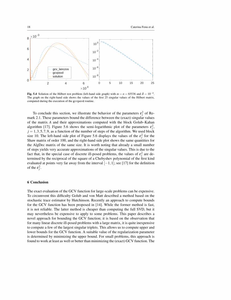
We finally consider two large-scale linear discrete ill-posed problems. Figure 5.4

displays results for a Hilbert matrix A ∈ R65536×65536. We use the noise level δ =

10−4. The Hilbert matrix is a well known Hankel matrix. We generate A by the smt li-

brary [30], which provides fast matrix-vector multiplication routines and compressed

storage for circulant and Toeplitz matrices. An extension to this library, available at

the web page of the package, implements an additional class for Hankel matrices.

The model solution is the one of the Baart test problem. We compare Algorithm 1

to the gcv lanczos method. The two computed solutions are fairly satisfactory, but

the one produced by our algorithm is clearly more accurate; see Table 5.2 and the

left-hand side graph of Figure 5.4. The gcvpsvd routine is particularly fast in this

example, because of the rapid decay of the singular values of the Hilbert matrix. This

is illustrated by the right-hand side graph of Figure 5.4. The method of the present pa-

per is faster in this and the following examples than the Quadrature method described

in [14]. We therefore do not compare with the latter method in Table 5.2.

The last linear system of equations that we discuss has a Toeplitz matrix A = [ai j]of order n = 65536, whose elements are defined by

ai j =2π

σ(4σ2 +(i− j)2).

This test matrix is denoted AlgDec in [30]. We let σ = 10. It is shown in [33] that

the asymptotic condition number, as n → ∞, is about 1027. We consider the model

solution from the Shaw problem and use the noise level δ = 10−2. This defines the

vector b in (1.1). The parameters of this experiment are reported in Table 5.2, while

Figure 5.5 displays the solution, a plot of the GCV function, and the decay of the

singular values of A. As in the previous example, Algorithm 1 is compared to the

gcv lanczos method. Table 5.2 shows this example to be particularly difficult for

Algorithm 1. The algorithm reached the last iteration allowed (k = 300) without sat-

isfying the convergence criterion. The long computation time is due to the very slow

decay of the singular values of the Gaussian matrix, but the solution obtained by the

gcvpsvd routine is much smoother than the one produced by gcv lanczos.


2 4 6

10 4

0

2

4

6

810 -3

gcv_lanczosgcvpsvdsolution

0 5 10 15 20 25

10 -8

10 -6

10 -4

10 -2

10 0

Fig. 5.4 Solution of the Hilbert test problem (left-hand side graph) with m = n = 65536 and δ = 10−4.

The graph on the right-hand side shows the values of the first 25 singular values of the Hilbert matrix,

computed during the execution of the gcvpsvd routine.

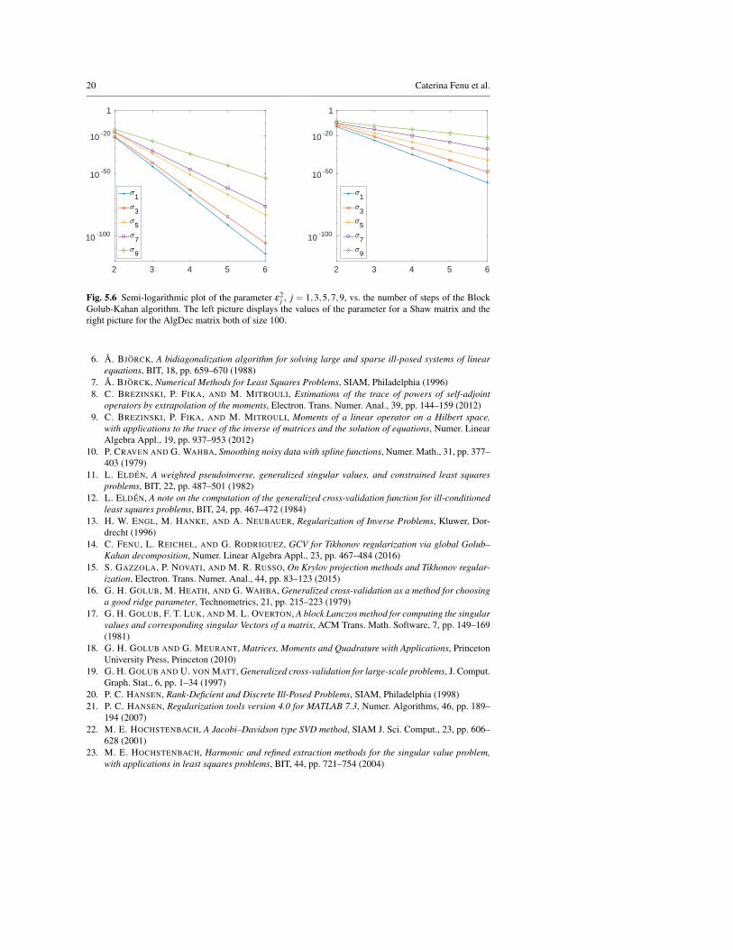
To conclude this section, we illustrate the behavior of the parameters ε2j of Re-

mark 2.1. These parameters bound the difference between the (exact) singular values

of the matrix A and their approximations computed with the block Golub–Kahan

algorithm [17]. Figure 5.6 shows the semi-logarithmic plot of the parameters ε2j ,

j = 1,3,5,7,9, as a function of the number of steps of the algorithm. We used block

size 10. The left-hand side plot of Figure 5.6 displays the values of the ε2j for the

Shaw matrix of order 100, and the right-hand side plot shows the same quantities for

the AlgDec matrix of the same size. It is worth noting that already a small number

of steps yields very accurate approximations of the singular values. This is due to the

fact that, in the special case of discrete ill-posed problems, the values of ε2j are de-

termined by the reciprocal of the square of a Chebyshev polynomial of the first kind

evaluated at points very far away from the interval [−1,1]; see [17] for the definition

of the ε2j .

6 Conclusion

The exact evaluation of the GCV function for large-scale problems can be expensive.

To circumvent this difficulty Golub and von Matt described a method based on the

stochastic trace estimator by Hutchinson. Recently an approach to compute bounds

for the GCV function has been proposed in [14]. While the former method is fast,

it is not reliable. The latter method is cheaper than computing the full SVD, but it

may nevertheless be expensive to apply to some problems. This paper describes a

novel approach for bounding the GCV function; it is based on the observation that

for many linear discrete ill-posed problems with a large matrix, it is quite inexpensive

to compute a few of the largest singular triplets. This allows us to compute upper and

lower bounds for the GCV function. A suitable value of the regularization parameter

is determined by minimizing the upper bound. For small problems, this approach is

found to work at least as well or better than minimizing the (exact) GCV function. The


2 4 6

10 4

0

0.5

1

1.5

2

2.5gcvpsvdsolution

2 4 6

10 4

0

0.5

1

1.5

2

2.5gcv_lanczossolution

10 -4 10 -2 10 0 10 2

10 -5

10 0

10 5

0 100 200 300

0.075

0.08

0.085

0.09

0.095

Fig. 5.5 Solution of the AlgDec test problem (graphs in the top row) with m = n = 65535 and δ = 10−2.

The graph on the left-hand side in the bottom row shows the GCV function V (µ) computed by Algo-

rithm 1; the graph on the right-hand side shows the first 300 singular values of the AlgDec matrix, com-

puted during the execution of the gcvpsvd routine.

proposed method performs particularly well when applied to the solution of linear

discrete ill-posed problems with a matrix, whose singular values decay to zero fairly

rapidly with increasing index number.

Acknowledgements The authors would like to thank Michiel Hochstenbach and a referee for comments.

Work of C.F and G.R. was partially supported by INdAM-GNCS.

References

1. H. AVRON AND S. TOLEDO, Randomized algorithms for estimating the trace of an implicit symmetric

positive semi-definite matrix, J. ACM, 58, pp. 8:1–8:34 (2011)

2. J. BAGLAMA, C. FENU, L. REICHEL, AND G. RODRIGUEZ, Analysis of directed networks via partial

singular value decomposition and Gauss quadrature, Linear Algebra Appl., 456, pp. 93–121 (2014)

3. J. BAGLAMA AND L. REICHEL, Restarted block Lanczos bidiagonalization methods, Numer. Algo-

rithms, 43, pp. 251–272 (2006)

4. J. BAGLAMA AND L. REICHEL, An implicitly restarted block Lanczos bidiagonalization method

using Leja shifts, BIT, 53, pp. 285–310 (2013)

5. Z. BAI, M. FAHEY, AND G. GOLUB, Some large-scale matrix computation problems, J. Comput.

Appl. Math., 74, pp. 71–89 (1996)


2 3 4 5 6

10 -100

10 -50

10 -20

1

1

3

5

7

9

2 3 4 5 6

10 -100

10 -50

10 -20

1

1

3

5

7

9

Fig. 5.6 Semi-logarithmic plot of the parameter ε2j , j = 1,3,5,7,9, vs. the number of steps of the Block

Golub-Kahan algorithm. The left picture displays the values of the parameter for a Shaw matrix and the

right picture for the AlgDec matrix both of size 100.

6. A. BJORCK, A bidiagonalization algorithm for solving large and sparse ill-posed systems of linear

equations, BIT, 18, pp. 659–670 (1988)

7. A. BJORCK, Numerical Methods for Least Squares Problems, SIAM, Philadelphia (1996)

8. C. BREZINSKI, P. FIKA, AND M. MITROULI, Estimations of the trace of powers of self-adjoint

operators by extrapolation of the moments, Electron. Trans. Numer. Anal., 39, pp. 144–159 (2012)

9. C. BREZINSKI, P. FIKA, AND M. MITROULI, Moments of a linear operator on a Hilbert space,

with applications to the trace of the inverse of matrices and the solution of equations, Numer. Linear

Algebra Appl., 19, pp. 937–953 (2012)

10. P. CRAVEN AND G. WAHBA, Smoothing noisy data with spline functions, Numer. Math., 31, pp. 377–

403 (1979)

11. L. ELDEN, A weighted pseudoinverse, generalized singular values, and constrained least squares

problems, BIT, 22, pp. 487–501 (1982)

12. L. ELDEN, A note on the computation of the generalized cross-validation function for ill-conditioned

least squares problems, BIT, 24, pp. 467–472 (1984)

13. H. W. ENGL, M. HANKE, AND A. NEUBAUER, Regularization of Inverse Problems, Kluwer, Dor-

drecht (1996)

14. C. FENU, L. REICHEL, AND G. RODRIGUEZ, GCV for Tikhonov regularization via global Golub–

Kahan decomposition, Numer. Linear Algebra Appl., 23, pp. 467–484 (2016)

15. S. GAZZOLA, P. NOVATI, AND M. R. RUSSO, On Krylov projection methods and Tikhonov regular-

ization, Electron. Trans. Numer. Anal., 44, pp. 83–123 (2015)

16. G. H. GOLUB, M. HEATH, AND G. WAHBA, Generalized cross-validation as a method for choosing

a good ridge parameter, Technometrics, 21, pp. 215–223 (1979)

17. G. H. GOLUB, F. T. LUK, AND M. L. OVERTON, A block Lanczos method for computing the singular

values and corresponding singular Vectors of a matrix, ACM Trans. Math. Software, 7, pp. 149–169

(1981)

18. G. H. GOLUB AND G. MEURANT, Matrices, Moments and Quadrature with Applications, Princeton

University Press, Princeton (2010)

19. G. H. GOLUB AND U. VON MATT, Generalized cross-validation for large-scale problems, J. Comput.

Graph. Stat., 6, pp. 1–34 (1997)

20. P. C. HANSEN, Rank-Deficient and Discrete Ill-Posed Problems, SIAM, Philadelphia (1998)

21. P. C. HANSEN, Regularization tools version 4.0 for MATLAB 7.3, Numer. Algorithms, 46, pp. 189–

194 (2007)

22. M. E. HOCHSTENBACH, A Jacobi–Davidson type SVD method, SIAM J. Sci. Comput., 23, pp. 606–

628 (2001)

23. M. E. HOCHSTENBACH, Harmonic and refined extraction methods for the singular value problem,

with applications in least squares problems, BIT, 44, pp. 721–754 (2004)


24. M. F. HUTCHINSON, A stochastic estimator of the trace of the influence matrix for Laplacian smooth-

ing splines, Commun. Statist. Simula., 18, pp. 1059–1076 (1989)

25. Z. JIA AND D. NIU, An implicitly restarted refined bidiagonalization Lanczos method for computing

a partial singular value decomposition, SIAM J. Matrix Anal. Appl., 25, pp. 246–265 (2003)

26. S. KINDERMANN, Convergence analysis of minimization-based noise level-free parameter choice

rules for linear ill-posed problems, Electron. Trans. Numer. Anal., 38, pp. 233–257 (2011)

27. S. MORIGI, L. REICHEL, AND F. SGALLARI, Orthogonal projection regularization operators, Nu-

mer. Algorithms, 44, pp. 99–114 (2007)

28. P. NOVATI AND M. R. RUSSO, A GCV based Arnoldi–Tikhonov regularization method, BIT, 54, pp.

501–521 (2014)

29. E. ONUNWOR AND L. REICHEL, On the computation of a truncated SVD of a large linear discrete

ill-posed problem, Numer. Algorithms, in press.

30. M. REDIVO–ZAGLIA AND G. RODRIGUEZ, smt: a Matlab toolbox for structured matrices, Numer.

Algorithms, 59, pp. 639–659 (2012)

31. M. Stoll, A Krylov–Schur approach to the truncated SVD, Linear Algebra Appl., 436, pp. 2795–2806

(2012)

32. J. TANG AND Y. SAAD, A probing method for computing the diagonal of the matrix inverse, Numer.

Linear Algebra Appl., 19, pp. 485–501 (2012)

33. C. V. M. VAN DER MEE AND S. SEATZU, A method for generating infinite positive self-adjoint test

matrices and Riesz bases, SIAM J. Matrix Anal. Appl., 26, pp. 1132–1149 (2005)

GCV for Tikhonov regularization by partial SVDreichel/publications/gcv.pdfGCV for Tikhonov...

Documents

Transcript of GCV for Tikhonov regularization by partial SVDreichel/publications/gcv.pdfGCV for Tikhonov...