Gavin Harrison - University of Leeds · Gavin Harrison Computer Science and Statistics Session:...
45
The candidate confirms that the work submitted is their own and the appropriate credit has been given where reference has been made to the work of others. I understand that failure to attribute material which is obtained from another source may be considered as plagiarism. (Signature of student) Summary and Application of Techniques in Constraint Programming Gavin Harrison Computer Science and Statistics Session: 2002/2003
Transcript of Gavin Harrison - University of Leeds · Gavin Harrison Computer Science and Statistics Session:...
The candidate confirms that the work submitted is their own and the appropriate credit has been givenwhere reference has been made to the work of others.
I understand that failure to attribute material which is obtained from another source may be consideredas plagiarism.
(Signature of student)
Summary and Application of Techniques inConstraint Programming
Gavin Harrison
Computer Science and Statistics
Session: 2002/2003
Summary and Application of Techniques in Constraint Programming
i
Summary
Recently it has become apparent that a powerful approach to programming, modelling and
problem solving can be developed. Different efforts in these areas can be exploited and
unified under a common and practical framework: Constraint Programming.
The aim of this project was to present a summary and application of techniques in Constraint
Programming.
The project has achieved its stated objectives by first providing a general background and a
description of the solution methods used. This framework is then used to apply Constraint
Programming methods to existing problems. Finally the use of industry standard software is
discussed.

Summary and Application of Techniques in Constraint Programming
ii
Acknowledgements
I would like to thank Sarah Fores for her help and advice throughout the whole duration of
this project as my supervisor. I would like to thank Tony Cohn for his constructive feedback
on my mid – project report and also for his advice given in the progress meeting. I would like
to thank Les Proll for his help with ILOG solver.
I would also like to thank my friends and family for helping me through this project with their
continuous support.

Summary and Application of Techniques in Constraint Programming
iii
Table of Contents1. INTRODUCTION.......................................................................................................................... 1
1.1 PROBLEM DEFINITION ................................................................................................................ 11.2 AIMS AND OBJECTIVES ............................................................................................................... 11.3 REACHING THE SOLUTION .......................................................................................................... 2
2. PROJECT BACKGROUND......................................................................................................... 2
2.1 INTRODUCTION ........................................................................................................................... 22.2 CONSTRAINTS............................................................................................................................. 32.3 CONFERENCES ............................................................................................................................ 4
3. SOLUTION METHODS ............................................................................................................... 5
3.1 CONSTRAINT SATISFACTION PROBLEMS (CSP) .......................................................................... 53.1.1 First Fail Principle .......................................................................................................... 63.1.2 Backtracking .................................................................................................................... 63.1.3 Under and Over Constrained Problems........................................................................... 73.1.4 Phase transition in CSPs.................................................................................................. 8
3.2 CONSTRAINT SOLVING (CS) ....................................................................................................... 9
4. APPLICATIONS OF CP .............................................................................................................. 9
4.1 INTRODUCTION ........................................................................................................................... 94.2 LOGIC PUZZLES ........................................................................................................................ 10
4.2.1 Example – SEND + MORE = MONEY.......................................................................... 104.2.2 Example – N-queens problem ........................................................................................ 134.2.3 Similarities and differences in Logic Puzzles................................................................. 14
4.3 EXISTING CP PROBLEMS........................................................................................................... 154.4 STABLE MARRIAGE PROBLEM .................................................................................................. 16
4.4.1 Existing Professional Approach to Solving SM ............................................................. 164.4.2 Past Project Attempt at Solving SM ............................................................................... 174.4.3 Definition of Personal Attempt at Solving SM ............................................................... 18
5. INDUSTRY STANDARD CP TOOLS....................................................................................... 23
5.1 CLP(R)..................................................................................................................................... 235.2 ILOG SOLVER .......................................................................................................................... 24
5.2.1 N-queens problem in ILOG Solver................................................................................. 245.2.2 Stable Marriage problem in ILOG Solver...................................................................... 25
6. EVALUATION ............................................................................................................................ 26
6.1 EVALUATION CRITERIA ............................................................................................................ 266.2 JUSTIFICATION OF THE CRITERIA .............................................................................................. 276.3 EVALUATION OF THE SOLUTION ............................................................................................... 28
6.3.1 Does the solution meet its goals and specified requirements?....................................... 286.3.2 Is the solution on time? .................................................................................................. 306.3.3 Is the solution reliable?.................................................................................................. 306.3.4 Is the solution maintainable?......................................................................................... 306.3.5 Does the solution satisfy the users? ............................................................................... 31
BIBLIOGRAPHY................................................................................................................................ 33
APPENDIX A – REFLECTION ON PROJECT EXPERIENCE ................................................... 34
APPENDIX B – PROJECT SCHEDULE.......................................................................................... 35
APPENDIX C – SAMPLE ILOG CODE........................................................................................... 36
APPENDIX D – UNIVERSITY ADMISSIONS PREFERENCE LISTS........................................ 40
Summary and Application of Techniques in Constraint Programming
1
1. Introduction
1.1 Problem Definition
This project will investigate a particular aspect of Operational Research and Artificial
Intelligence, namely Constraint Programming. The area of Constraint Programming can be
sub-divided further and explained in detail (see sections 2 and 3). Constraint Programming
can be used to solve a variety of problems, both artificial and real (see section 4).
These methods of Constraint Programming can be applied through applications or software.
Pieces of Industry Standard Software and their benefits can be discussed in more detail (see
section 5).
An examples based approach is adopted for this project, since it will present a clearer
understanding. With this in mind, wherever a substantial element of theory is encountered, a
small example will be offered alongside. Later on, when tackling some more complex
problems, existing approaches to solving the problems will be offered. A personal take on an
already existing Constraint Programming problem will also be offered (Section 4).
The project relates to a number of modules provided by the School of Computing. The
modules OR21 – Linear Programming and OR22 – Decision Modelling, which have been
previously studied, form the basis of knowledge required in Operational Research for the
project. More advanced modules, which have been studied along side the project and are
immediately relevant include and OR31 – Discrete Optimisation and OR32 – Scheduling:
Models and Algorithms. Additionally CO33 – Algorithms and Complexity, which has been
studied, should provide awareness of time complexity and running times.
1.2 Aims and Objectives
The aim of the project is:
• Present a Summary and Application of Techniques in Constraint Programming
In order for this general aim to be fulfilled the natural evolution of the project would be to
tackle the following Minimum Requirements:
• To present recent sources of information on Constraint Programming techniques.
• To present an existing approach to solving a Constraint Programming problem.
• To present how to use industry standard software (e.g. iLOG) for solving simple
Constraint Programming problems.

Summary and Application of Techniques in Constraint Programming
2
The minimum requirements of the project could be exceeded by:
• Presenting an alternative approach to the specified Constraint Programming problem.
• Presenting the solution of an existing Constraint Programming problem using industry
standard software.
1.3 Reaching the Solution
These requirements can be achieved by presenting the solution under different sections and in
a logical order. A project background chapter (section 2) should first be established to
introduce the topic and should also contribute towards the present recent sources of
information requirement somewhat. A more specific solution methods chapter (section 3) will
follow which will detail the basic methods used to solve standard Constraint Programming
problems, which should satisfy the present recent sources of information minimum
requirement. Existing problems and their solutions are then discussed in a separate
applications chapter (section 4), which should satisfy the present an existing approach
requirement. The expansion opportunity of an alternative approach to an existing Constraint
Programming problem should be included in section 4. The industry standard software
requirement will be tackled in a software discussion chapter (section 5), and is also where the
solution of an existing Constraint Programming problem using industry standard software
expansion opportunity should be discussed. This strategy relates to the original strategy
outlined in the mid-project report phase, which itself is included in Appendix B for reference
purposes.
2. Project Background
2.1 Introduction
First of all let the question of ‘What is Constraint Programming (CP)?” be addressed. Barták
(1998) suggests that CP is an emergent technology for declarative description, and goes on to
state that CP is used for “effective solving of large, particularly combinatorial, problems
especially in areas of planning and scheduling.” Barták (1998) did actually state that CP is a
software technology, when in fact CP is more of a technique used to solve problems, often
with the use of software technology.
Using ideas proposed by Barták (1998) to tackle the issue ‘what CP is used for’, it can be
suggested that the idea of constraint programming is to solve problems by stating constraints
(conditions, properties) – see 2.2, which must be satisfied by the solution. The area of CP
originated in the sixties and seventies in the areas of Artificial Intelligence and Computer
Graphics. Recently (in the last ten years) it has become apparent that a powerful approach to
Summary and Application of Techniques in Constraint Programming
3
programming, modelling and problem solving can be developed. Different efforts in these
areas can be exploited and unified under a common and practical framework: Constraint
Programming.
Recent applications of CP as suggested by Barták (1998) include:
• computer graphics (to express geometric coherence in the case of scene analysis)
• natural language processing (construction of efficient parsers)
• database systems (to ensure and/or restore consistency of the data)
• operational research problems (like optimisation problems)
• molecular biology (DNA sequencing)
• business applications (option trading)
• electrical engineering (to locate faults)
• circuit design (to compute layouts), etc.
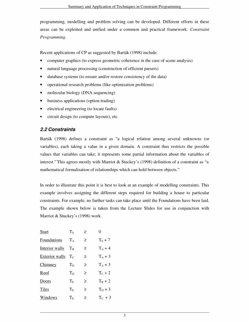
2.2 Constraints
Barták (1998) defines a constraint as “a logical relation among several unknowns (or
variables), each taking a value in a given domain. A constraint thus restricts the possible
values that variables can take; it represents some partial information about the variables of
interest.” This agrees mostly with Marriot & Stuckey’s (1998) definition of a constraint as “a
mathematical formalisation of relationships which can hold between objects.”
In order to illustrate this point it is best to look at an example of modelling constraints. This
example involves assigning the different steps required for building a house to particular
constraints. For example, no further tasks can take place until the Foundations have been laid.
The example shown below is taken from the Lecture Slides for use in conjunction with
Marriot & Stuckey’s (1998) work.
Start TS ≥ 0
Foundations TA ≥ TS + 7
Interior walls TB ≥ TA + 4
Exterior walls TC ≥ TA + 3
Chimney TD ≥ TA + 3
Roof TD ≥ TC + 2
Doors TE ≥ TB + 2
Tiles TE ≥ TD + 3
Windows TE ≥ TC + 3
Summary and Application of Techniques in Constraint Programming
4
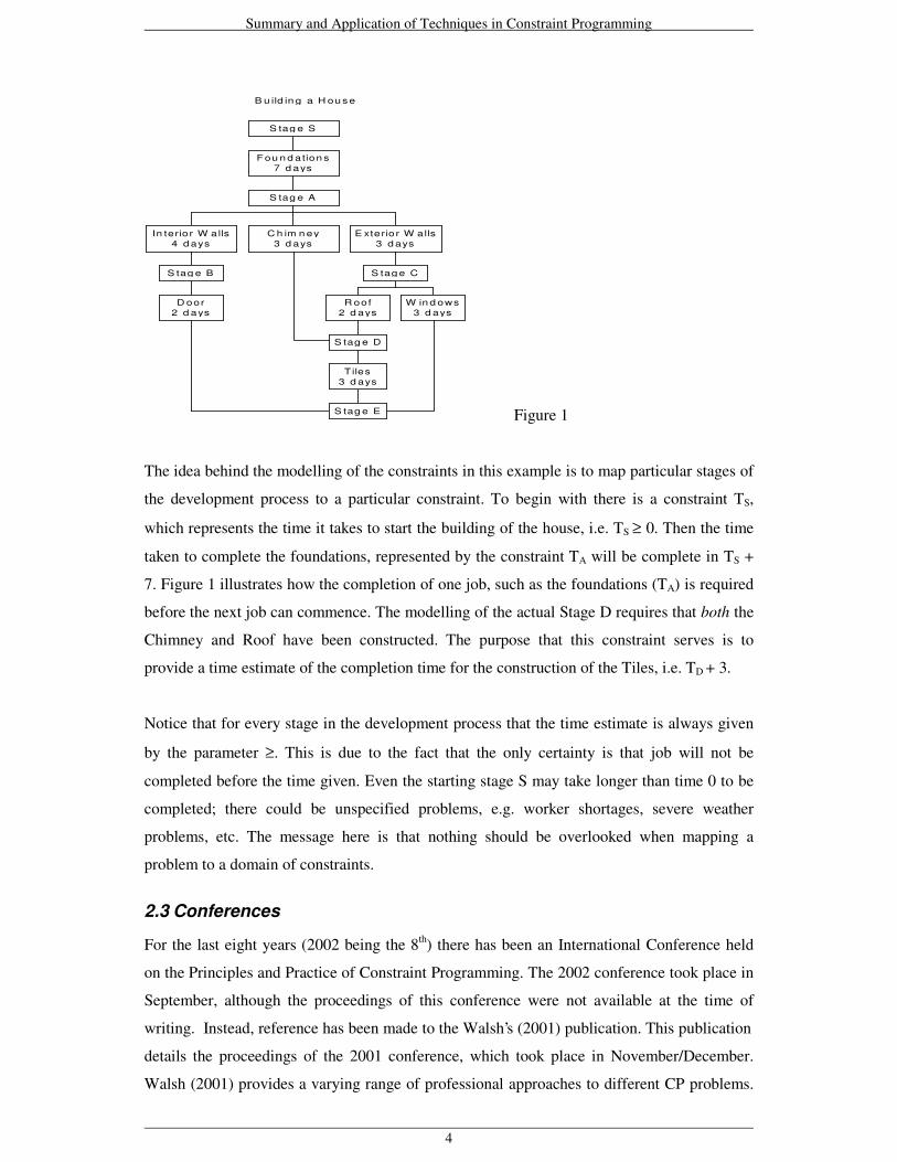
B u ild in g a H ou s e
D oor2 d ays
S tag e B
In terio r W alls4 d ays
C h im n ey3 d ays
S tag e E
Tiles3 d ays
S tag e D
R oof2 d ays
W in d ows3 d ays
S tag e C
E xterio r W alls3 d ays
S tag e A
F ou n d ation s7 d ays
S tag e S
Figure 1
The idea behind the modelling of the constraints in this example is to map particular stages of
the development process to a particular constraint. To begin with there is a constraint TS,
which represents the time it takes to start the building of the house, i.e. TS ≥ 0. Then the time
taken to complete the foundations, represented by the constraint TA will be complete in TS +
7. Figure 1 illustrates how the completion of one job, such as the foundations (TA) is required
before the next job can commence. The modelling of the actual Stage D requires that both the
Chimney and Roof have been constructed. The purpose that this constraint serves is to
provide a time estimate of the completion time for the construction of the Tiles, i.e. TD + 3.
Notice that for every stage in the development process that the time estimate is always given
by the parameter ≥. This is due to the fact that the only certainty is that job will not be
completed before the time given. Even the starting stage S may take longer than time 0 to be
completed; there could be unspecified problems, e.g. worker shortages, severe weather
problems, etc. The message here is that nothing should be overlooked when mapping a
problem to a domain of constraints.
2.3 Conferences
For the last eight years (2002 being the 8th) there has been an International Conference held
on the Principles and Practice of Constraint Programming. The 2002 conference took place in
September, although the proceedings of this conference were not available at the time of
writing. Instead, reference has been made to the Walsh’s (2001) publication. This publication
details the proceedings of the 2001 conference, which took place in November/December.
Walsh (2001) provides a varying range of professional approaches to different CP problems.
Summary and Application of Techniques in Constraint Programming
5
One specific study from Walsh’s (2001) publication is discussed later on in this investigation
– see 4.4.1 for details. The various investigations provided by Walsh (2001) are the latest
innovations and practices in the area of CP and as such assume knowledge of the basics of
certain related topics. Marriot & Stuckey (1998) present a detailed guide on CP, which would
compliment the investigations provided in Walsh’s (2001) publication.
Other conferences, which include research in CP that have taken place recently, include:
• The Practical Application of Constraint Technology [Malyshkin (Ed) 2001].
• International Joint Conference on Artificial Intelligence [Nebel (Ed) 2001]
• European Conference on Artificial Intelligence [Horn (Ed) 2000]
• International Conference on Logic Programming [Stuckey (Ed) 2002]
3. Solution Methods
Once a problem has been modelled by constraints it then needs to be solved. There are two
main approaches, which are used when dealing with solving constraints in CP: Constraint
Satisfaction and Constraint Solving.
3.1 Constraint Satisfaction Problems (CSP)
The CSP is a problem where one is given:
• a finite set of variables,
• a function which maps every variable to a finite domain,
• a finite set of constraints.
Each constraint restricts the combination of values that a set of variables may take
simultaneously. A solution of a CSP is an assignment of a value to each variable, which
satisfies all the constraints and where each variable must take a value from its domain. The
task is to find one solution or all solutions.
Barták (1998) implies that the CSP is a combinatorial problem, which can be solved by search
methods. A trivial algorithm called generate and test exists, which generates all possible
combinations of values, and then tests each combination of values to check if it satisfies all
the constraints. This algorithm an expensive approach to solving any problem; as a result,
most of the research areas in CP involve trying to find a more efficient way of solving a given
problem.

Summary and Application of Techniques in Constraint Programming
6
There are many different heuristics and techniques used in CSPs, generate and test being just
one of these. The following sections discuss some of these in more detail.
3.1.1 First Fail Principle
This heuristic is described by Marriott & Stuckey (1998) and Barták (1998) as “To
succeed, try first where you are most likely to fail”. The idea behind this principle is
the order in which to try the different domain values. If the smallest domain is
chosen, then the branching factor is limited, allowing the failure of an entire branch to
be determined quickly so that a search can be conducted in more profitable areas.
This is a basic Depth First Search (DFS) approach to solving a Branch and Bound (B
& B) problem. The First Fail principle could be applied to an area like the N-queens
problem and will be once the N-queens problem has been discussed (4.2.2).
3.1.2 Backtracking
This is a technique concerned with determining the satisfiability of a CSP. An initial
attempt at determining the satisfiability of a CSP could be to use a ‘brute force
approach’ (Marriot & Stuckey 1998) by searching through all the combinations of
different values, since the number of combinations is of finite value. However, it
should be remembered that the process of solving CSPs is NP-hard. Alternatively, a
more effective approach would be to use a backtracking technique. One such instance
of this is chronological backtracking as defined by Marriott & Stuckey (1998).
The idea behind chronological backtracking is to determine satisfiability of a CSP by
choosing a variable, and then for each variable in its domain, determining
satisfiability of the constraint which results by replacing the variable with that value.
This is achieved by recursively calling the backtracking algorithm and by making use
of the parametric function satisfiable (c). This takes a primitive constraint c that
involves no variables and returns true or false indicating whether c is satisfiable or
not. Marriott & Stuckey (1998) provide an example of the chronological
backtracking algorithm in use, which is shown below.
• Consider the CSP consisting of the constraint X < Y ^ Y < Z and the variables X,
Y, Z each with domain {1, 2}.
• The first step in the algorithm is to choose a variable in the constraint, say X and
then iterate through the domain of X {1, 2}.
• 1 replaces X in the constraint to give 1 < Y ^ Y < Z.

Summary and Application of Techniques in Constraint Programming
7
• A call is then made to the partial_satisfiable procedure, which states that this new
constraint is partially satisfiable.
• The backtracking algorithm is then called, which results in another variable, say
Y being chosen, again with the domain {1, 2}
This process continues until one of the constraints is violated (noting the strict <
inequality). When this occurs, a different domain is selected for the variable, which
just caused the violation. A false statement is returned whenever a combination of
values is not satisfiable based on the constraints. The search tree for this example is
given below.
F ig u re 2 : S earch tree for th e b ack track in g exam p le
X =1 X =2
Y=1 Y=2 Y=1 Y=2
Z=1 Z=2
fa lse
fa lse fa lse
1 < 2 ^ 2 < Z
1 < Y ^ Y < Z
fa lse fa lse
2 < Y ^ Y < Z
X < Y ^ Y < Z
The drawback of the backtracking technique is that in the worst case it has an
exponential time complexity, which is to be expected since this is a complete solver.
The alternative choices offered at different stages will lead to different search trees.
Compare this to a heuristic technique such as the first fail principle (3.1.1); this can
produce much smaller search trees, although for the general problem the worst case
time complexity still remains exponential.
These are widely used techniques in Constraint Programming and indeed in many other areas
of computation, which can be applied to areas like the N-queens problem or the Stable
Marriage problem, which shall be discussed in greater depth later. There are many other
techniques that exist for the solving of CSPs such as forward checking, look ahead and
heuristics like succeed first as Barták (1998) suggests.
3.1.3 Under and Over Constrained Problems
When a CP problem has been defined it is likely to fall into one of two distinct
categories; these being under constrained problems and over constrained problems.

Summary and Application of Techniques in Constraint Programming
8
An under constrained instance occurs when a problem has few constraints or when all
the constraints are easy to solve, often resulting in many relatively easy solutions to
the given problem. An over constrained instance occurs when a problem has many
constraints or when some of the constraints are hard to solve. A constraint, which is
hard to solve is most likely NP-hard, so a traditional approach to solving the given
problem is impossible (in polynomial time).
While an over-constrained system cannot be solved via traditional methods, it is
possible to extend or alter the original problem so that a general idea of the solution
(to the original problem) can be formulated. Barták (1998) suggests Extending CSP
and Partial CSP as possible methods for solving over constrained problems, and goes
on to suggest Constraint Hierarchies as an alternative method. The Extending and
Partial methods are contrasting styles. The Extending method takes a problematic
constraint and extends it to include a new parameter or requirement, whereby the
solution is solved based on this new requirement. The Partial method reduces a
problematic constraint so that it is similar to an existing problem that is known to be
solvable in polynomial time. Constraint Hierarchies involve the definition of hard
constraints and soft constraints, where a hard constraint is one which must be
included in the solution to the problem and a soft constraint is one which should, but
doesn’t necessarily have to be included in the solution to the problem.
3.1.4 Phase transition in CSPs
In reflection of section 3.4.3 there clearly must be some kind of area that separates an
under constrained problem from an over constrained problem. Grant (1997) suggests
that a CSP can be shown to exhibit a phase transition. So it would seem that the area
separating these two phases of under constrained and over constrained can be
referred to as a ‘region’ (Grant 1997). This region is called the Phase Transition
Region. Phase transition is a process that was first recognised in graph colouring
problems by Cheeseman et al (1991). This transition lies between a region where
almost all problems have many solutions and are easy to solve, and a region where
almost all problems have no solution and their insolubility is relatively easy to prove.
Problems that occur in this phase transition region are typically the most difficult kind
of problem. The reason why problems in the phase transition region are the most
difficult is because the nature of a solution attempt is unknown prior to starting. An
under constrained problem would involve finding a solution, whereas a over
constrained problem would involve proving that no feasible solution can be obtained

Summary and Application of Techniques in Constraint Programming
9
in polynomial time. Then the question must be posed as to what approach a solution
(or proof) would take. There is no right answer to this question, so choosing on a
method, which appears to be the best in the hope that it is correct may be a feasible
approach. There are of course detailed methods for dealing with problems which lie
in the phase transition region, which is mainly what Grant’s (1997) work is
investigating. The phase transition procedure could be used to separate easy and hard
problems for CSP algorithms.
Creignou et al (2001) state that, “One of the fundamental goals of the theory of computation,
or ‘complexity theory’, is to determine how much of a computational resource is required to
solve a given computational task. Along the way it postulates definitions of when a task is
computationally ‘easy’ and when it is, or likely to be ‘hard’.” This is a very important aspect
of computation and is key when considering an appropriate algorithm to solve a particular
problem.
3.2 Constraint Solving (CS)
Barták (1998) states that “Constraint Solving differs from Constraint Satisfaction by using
variables with infinite domains. Also, the individual constraints are more complicated, e.g.,
non-linear equalities. Consequently, the constraint solving algorithms use algebraic and
numeric methods instead of combinations and search. However, there exists an approach
which discretises the infinite domain into a finite number of components and then applies the
techniques of constraint satisfaction.”
This approach to solving the constraints formulated is much more complicated than the
method used for CSP. As a result of this it would be best to use CSP for the solving of the
problem where possible. However, the vast majority of real-world cases will involve infinite
domains, and as such cannot be solved realistically by the method of CSP. In these situations
it would be necessary to adopt the CS approach.
4. Applications of CP
4.1 Introduction
Another area of interest is where CP is used. Barták (1998) suggests that there are several
corporations, which make use of Constraint Technology such as British Airways, SAS,
Swissair, French railway authority SNCF, Hong Kong International Terminals and Michelin.
These companies have realised how much quicker Constraint Technology speeds up the
planning stage of any job. Obviously there will be a certain period of time before the

Summary and Application of Techniques in Constraint Programming
10
methodology is fully assimilated into the day-to-day running of the business. This period of
time will come in the form of teaching the new method to staff and/or teaching the operation
of a piece of software, which uses the method of constraints to staff. As would be expected,
the larger the company the more costly (in terms of time and money) the method is to
introduce.
While the introduction costs of a new methodology will be a key concern of any corporation,
the big picture will out-shadow this. That is, how much time and money is saved using the
technology in the long run. In most cases this should be beneficial.
In order to explore the application of CP more fully, looking at artificial examples and logic
puzzles will be the best approach.
4.2 Logic Puzzles
These are logic puzzles or artificial problems, although they will make much clearer some of
the issues discussed in previous sections. Some types of logic puzzles, solvable by the method
of CP are:
• N-queens
• Zebra (five house puzzle)
• a crossword puzzle
• cryptoarithmetics (SEND+MORE=MONEY)
First of all the SEND+MORE=MONEY, cryptoarithmetic puzzle shall be demonstrated.
4.2.1 Example – SEND + MORE = MONEY
Problem Definition
This is the problem of assigning different numerals to each of the letters in the words
SEND, MORE and MONEY, where S and M cannot be assigned to zero. The idea is
that when the string of numerals corresponding to the word MORE is added to the
string of numerals corresponding to the word MORE, then the solution will be the
string of numerals corresponding to the word MONEY. More algebraically, this is
what is required:
S E N D
+ M O R E
M O N E Y

Summary and Application of Techniques in Constraint Programming
11
Why CP?
In order to solve this problem, it is beneficial to impose a number of constraints onto
the set of variables. The set of constraints produced provides a preferable approach to
solving the problem than that of total enumeration.
Solving the problem
Part of the solution to this problem draws upon the possibility of a carry bit when the
numerals are added together. Say D = 8 and E = 9, then Y = 7 (the 1 is carried over
into the tens column to add to that constraint. Let there be three carry bits defined, P1,
P2 and P3 where these contribute to the constraints imposed on the tens, hundreds
and thousands columns respectively. The problem is re-defined algebraically with the
carry bits imposed below.
P3 P2 P1
S E N D
+ M O R E
M O N E Y
Barták (2002) suggests the following constraint model to solve this problem.
E,N,D,O,R,Y in 0..9, S,M in 1..9, P1,P2,P3 = 0 or 1
all_different (S,E,N,D,M,O,R,Y)
D + E = 10*P1 + Y [R1]
P1 + N + R = 10*P2 + E [R2]
P2 + E + O = 10*P3 + N [R3]
P3 + S + M = 10*M + O [R4]
From this it is possible to attach values to each letter in steps, as shown below to
eventually achieve the solution.
• P3 + S + M = 10*M + O [R4]
M = 1, since P3 + S + M ≤ 18, i.e. 1 + 9 + 8 = 18. So M = 1, since it cannot equal
0
• P3 + S + 1 = 10 + O [R4]
1 + S + 1 = 10 + O [R4] if P3 = 1, so (S = 8 and O = 0) or (S = 9 and O = 1)
0 + S + 1 = 10 + O [R4] if P3 = 0, so (S = 9 and O = 0)
M = 1, so O = 0. Consideration of [R3] should help work out the value of S, but
start with S = 8 for now.

Summary and Application of Techniques in Constraint Programming
12
• P2 + E + O = 10*P3 + N [R3]
P2 + E =10 + N [R3]
E = 10 + N [R3] if P2 = 0, impossible since would require E ≥ 10
E = 9 + N [R3] if P2 = 1, also impossible since would require N = 0 and O = 0
Now can set S = 9 and P3 = 0
• P2 + E + O = 10*P3 + N [R3]
P2 + E = N [R3]
E cannot equal N so P2 = 1
1 + E = N [R3]
Let constraint [R2] be considered now and return to E and N later.
• P1 + N + R = 10*P2 + E [R2]
P1 + E + 1 + R = 10 + E [R2]
E + 1 + R = 10 + E [R2] if P1 = 0, so R = 9, which is impossible since S = 9
1 + E + 1 + R = 10 + E [R2] if P1 = 1, so R = 8 and can fix P1 = 1
• Now the digits remaining are 2, 3, 4, 5, 6 and 7
D + E ≥ 12 since P1 = 1 and 0 and 1 values are unavailable
D + E ≥ 12 can only be satisfied by {5,7} or {6,7} values for combination of D
and E values
So D = 7 since E ≠ 7 as would require N = 8 (by N = E + 1) which is already
taken
E = 5 (N = E + 1 = 6) or E = 6 (N = E + 1 = 7: already taken), so E = 5, N = 6 and
Y = 2 since D + E = 10*P1 + Y [R1]
So the final solution to the problem is given by:
0 1 1
9 5 6 7
+ 1 0 8 5
1 0 6 5 2

Summary and Application of Techniques in Constraint Programming
13
4.2.2 Example – N-queens problem
Problem Definition
Marriot & Stuckey (1998) pp.86 suggest that this is the problem of placing N queens
on a chessboard of a size N × N so that no queen can capture another queen. Consider
the 4-queens problem. We can formalise this as a CSP by associating with the ith
queen two variables, Ri and Ci, which are, respectively, its row and column position
on the board. The domain of each variable is {1,2,3,4}.
Why CP?
As with the SEND + MORE = MONEY problem (4.2.1) this problem lends itself
well to be solved by the method of CP. A number of constraints are necessary to
successfully apply this problem to CP, which restrict the placement of queens on the
board (once a queen has been placed).
Solving the problem
Marriot & Stuckey (1998) propose the following set of constraints:
• R1 ≠ R2 ^ R1 ≠ R3 ^ R1 ≠ R4 ^ R2 ≠ R3 ^ R2 ≠ R4 ^ R3 ≠ R4,
Which ensures that no two queens can be in the same row.
• C1 ≠ C2 ^ C1 ≠ C3 ^ C1 ≠ C4 ^ C2 ≠ C3 ^ C2 ≠ C4 ^ C3 ≠ C4
Which ensures that no two queens can be in the same column.
• C1 - R1 ≠ C2 - R2 ^ C1 - R1 ≠ C3 - R3 ^ C1 - R1 ≠ C4 - R4 ^ C2 - R2 ≠ C3 - R3
^ C2 - R2 ≠ C4 - R4 ^ C3 - R3 ≠ C4 - R4
And
C1 + R1 ≠ C2 + R2 ^ C1 + R1 ≠ C3 + R3 ^ C1 + R1 ≠ C4 + R4 ^ C2 + R2 ≠ C3
+ R3 ^ C2 + R2 ≠ C4 + R4 ^ C3 + R3 ≠ C4 + R4
Enforce that no two queens are on the same diagonal.
One solution to the 4-queens problem is shown in Figure 3.
Figure 3

Summary and Application of Techniques in Constraint Programming
14
The First Fail principle (3.1.1) could also be applied to the N-queens problem. By
this principle an attempt would be made to try placing the first queen in one of the
four centre squares of the chessboard if the N value was an even number. This would
block off more spaces than any other position(s) on the chessboard. If the N value
was an odd number then there would be one centre square instead of four. The
example is better illustrated by Figure 4, below, which shows a 4-queens problem.
Q = Queen X = Space covered by a queen
Step 1 Step 2 Step 3
X X X X X X Q X X X Q
X Q X X X Q X X X Q X X
X X X X X X X X X X X
X X X X X X X Q X
Figure 4
• Step 1: Place a queen in one of the centre squares; this blocks off twelve squares
including the queens square. It is evident from this point that a solution cannot be
derived, since only two positions are left for queens (one queen per row and
column).
• Step 2: Place a second queen on the square that blocks off the highest number of
additional spaces; any choice of square here blocks off three additional squares.
• Step 3: There is only one square left and two queens left to place, so the process
could finish here. For illustrative purposes a queen was placed in the last
remaining square to show a fully covered chessboard. This process would result
in the elimination of this square and the other three centre squares from the search
tree as a starting point for a queen.
The first-fail approach is a reasonable strategy for small problems like this one, since
it would be relatively quick to find a solution. For larger problems, the first-fail
principle is an unrealistic approach, since it may take an exponential amount of time
to find a solution.
4.2.3 Similarities and differences in Logic Puzzles
The logic puzzles shown in 4.2.1 and 4.2.2 are just some of many different types.
With the SEND + MORE = MONEY case, variables are applied to each of the
different letters. By doing this, a certain number of constraints can then be derived
based on the values that these variables take. Eventually the constraint of SEND +

Summary and Application of Techniques in Constraint Programming
15
MORE = MONEY is satisfied as shown in 4.2.1, where the solution given is the only
possible solution to this problem.
The N-queens problem (4.2.2) in contrast to the SEND + MORE = MONEY problem
can have several solutions and uses a different method of applying constraints. Here,
it would be impractical to apply the same method as for the SEND + MORE =
MONEY case. Say, for example that variables are mapped to each individual queen,
then it would clearly be difficult to satisfy the existing constraints to solve the
problem as shown in 4.2.2. Equivalently it wouldn’t be a good idea to apply variables
to each individual square, since there would be far too many to manage, especially as
the size of N increases.
Consideration of the number of variables a particular problem will require to solve (or
attempt to solve) a particular problem is important. So the choice of variables will
often lead to an under-constrained problem or an over-constrained problem (see
3.1.3). When attempting to solve other logic puzzles it will be important to identify a
suitable number of variables to solve the constraints that the problem implies. A
formulation of a given problem would preferably not be in the over-constrained
region (otherwise the problem couldn’t be solved in its present form).
If a (partial) solution to an over-constrained problem is desired then the problem will
have to be relaxed or weakened. Once a reduced form of the original problem has
been formed, which is solvable in polynomial time, then a (partial) solution could be
obtained.
4.3 Existing CP problems
As outlined above, CP techniques can be very useful tools when tackling logic puzzles. There
are also many real world problems that can be formulated as CP problems. For example, CP
techniques can be applied to Network Flow problems [Bockmayr et al 2001]. In this case a
Flow Constraint is introduced, which has the following form:
Flow (NodeType, Edge, Conv, EdgeCost, NodeCost, Demand, Flow, FlowVal)
This is an example of an instance when CP isn’t the most ideal approach, since as stated by
Bockmayr et al (2001), “constraint programming systems do not provide special support to
deal with network flows.” In spite of this Bockmayr et al (2001) produce the global constraint
flow for the modelling and solving network problems inside constraint programming.
Summary and Application of Techniques in Constraint Programming
16
On the other hand there are plenty of problems, which lend themselves well to CP
methodologies. Specifically the Stable Marriage problem is well suited to the CP framework.
Briefly (since Stable Marriage will be discussed in more detail in section 4.4), Stable
Marriage involves an equal number of men and women who are all looking for partners of the
opposite sex. The aim is to provide a complete set of ideal pairs of couples (whereby each
individual is matched with their ideal partner). This ideal as will be indicated later is quite
unlikely, so a constraint imposed on the problem may be a numerical requirement to the
number of stable matchings.
In a standard Stable Marriage problem there are an equal number of men and women. In a
real world situation the number of men and women is unlikely to be equal. A constraint would
need to be applied to this situation whereby all members of the sex with the smallest
population are contained in a matching. When the numbers are unequal like this a deficit of
unmatched individuals is a certainty.
4.4 Stable Marriage Problem
One specific application of CP methodologies is to the Stable Marriage problem. The
classical Stable Marriage problem (SM) as defined in Walsh’s (2001) publication p225,
comprises n men and n women, where each person has a preference list in which they rank all
members of the opposite sex in strict order. A matching M is a bijection between the men and
women. A man mi and a woman wj form a blocking pair for M if mi prefers wj to his partner in
M and wj prefers mi to her partner in M. A matching that admits no blocking pair is said to be
stable, otherwise the matching is unstable. SM arises in important practical applications, such
as the annual match of graduating medical students to their first hospital appointments in a
number of countries.
4.4.1 Existing Professional Approach to Solving SM
Walsh’s (2001) publication provides a recent investigation into an approach to the
solving of the SM problem. Specifically Gent et al (2001) provide two approaches to
solving the problem; a classical SM approach and an instance I of SM. The SM
instance I approach involves the use of the Extended Gales/ Shapley (EGS)
algorithm. The principal of this algorithm is to delete certain (man, woman) pairs
from the preference lists that cannot belong to a stable matching.
Gent et al (2001) go on to introduce the concept of conflict matrices. This is best
explained by a simple illustrative example, Figure 5, below.
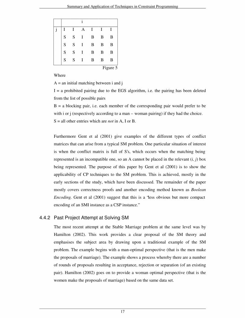
Summary and Application of Techniques in Constraint Programming
17
i
j I I A I I I
S S I B B B
S S I B B B
S S I B B B
S S I B B B
Figure 5
Where
A = an initial matching between i and j
I = a prohibited pairing due to the EGS algorithm, i.e. the pairing has been deleted
from the list of possible pairs
B = a blocking pair, i.e. each member of the corresponding pair would prefer to be
with i or j (respectively according to a man – woman pairing) if they had the choice.
S = all other entries which are not in A, I or B.
Furthermore Gent et al (2001) give examples of the different types of conflict
matrices that can arise from a typical SM problem. One particular situation of interest
is when the conflict matrix is full of S’s, which occurs when the matching being
represented is an incompatible one, so an A cannot be placed in the relevant (i, j) box
being represented. The purpose of this paper by Gent et al (2001) is to show the
applicability of CP techniques to the SM problem. This is achieved, mostly in the
early sections of the study, which have been discussed. The remainder of the paper
mostly covers correctness proofs and another encoding method known as Boolean
Encoding. Gent et al (2001) suggest that this is a “less obvious but more compact
encoding of an SMI instance as a CSP instance.”
4.4.2 Past Project Attempt at Solving SM
The most recent attempt at the Stable Marriage problem at the same level was by
Hamilton (2002). This work provides a clear proposal of the SM theory and
emphasises the subject area by drawing upon a traditional example of the SM
problem. The example begins with a man-optimal perspective (that is the men make
the proposals of marriage). The example shows a process whereby there are a number
of rounds of proposals resulting in acceptance, rejection or separation (of an existing
pair). Hamilton (2002) goes on to provide a woman optimal perspective (that is the
women make the proposals of marriage) based on the same data set.

Summary and Application of Techniques in Constraint Programming
18
The main limitation of the solution given by Hamilton (2002) is that only one
example is given. One problem, which can occur in a SM problem is the time it takes
to find a stable marriage. A larger example (in addition to the one already given)
would have better portrayed the difficulties of finding a stable marriage; in this
example a person is only rejected at most once, which is quite unlikely in a typical
SM problem. Another area of the SM problem that could have been explored was the
concept of unbalanced men and women (where there are an unequal number of men
and women).
4.4.3 Definition of Personal Attempt at Solving SM
An example of how the SM problem can begin to be applied to a practical situation
will now be discussed. One such possible application is that of a University
Admissions problem. The problem consists of a number of universities (each of
which has a number of courses) and a number of students (or potential students).
Each student can make up to six choices of course and each course has a maximum
number of places to be filled. Each student will have his/her own preference of
courses from the six they previously selected. The preference list for each student is
likely to be made up of a number of different factors, which could range from
common factors like nightlife and job prospects to other factors more specific to an
individual student. The approach to solving the problem will assume that each student
has his or her own clear preference list defined.
Similarly, the admissions department at each university will have their own
preference list of students made up from a number of different factors. The added
difficulty for the university is that it will be accepting admissions for a number of
different courses, each of which will most likely have different sized limits on the
number of places available.
A simple instance of the problem will be given to begin with, leaving scope for the
addition of further constraints to the problem gradually. Initially let the problem be
tackled as a classical stable marriage problem, with an identical number of students to
the number of courses. It makes sense to assume that the students make the initial
proposals, since universities don’t have full access to a comprehensive list, which
details all potential students. A first attempt below shows a stable marriage instance
with four students and four courses (each with one placement each).

Summary and Application of Techniques in Constraint Programming
19
First Attempt
Let Si denote Student i and Ci denote Course i.
The preference lists for each of the four students are given below.
S1 (C1, C2, C3, C4)
S2 (C2, C4, C1, C3)
S3 (C1, C3, C2, C4)
S4 (C1, C4, C3, C2)
The preference lists for each of the four courses is given below.
C1 (S3, S1, S2, S4)
C2 (S3, S2, S1, S4)
C3 (S1, S3, S4, S2)
C4 (S3, S1, S4, S2)
Since this is a classical instance of the stable marriage, the students will propose their
interests in courses in rounds, starting with the most preferable.
Round1
• S1, S3 and S4 propose an interest in course C1
• S2 proposes an interest in course C2
which results in
• C1 accepting S3’s (stable marriage) proposal
• C1 rejecting the proposal of S1 and S4
• C2 accepting S2’s proposal (stable since S3 already has their first choice)
Round 2
• S1 proposes an interest in course C2
• S4 proposes an interest in course C4
which results in
• C2 rejecting S1’s proposal
• C4 accepting S4’s proposal
Round 3
• S1 proposes an interest in course C3
which results in
• C3 accepting S1’s proposal
Summary and Application of Techniques in Constraint Programming
20
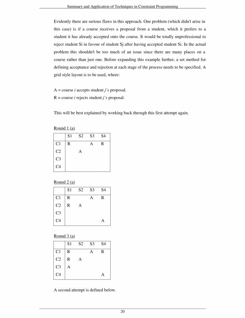
Evidently there are serious flaws in this approach. One problem (which didn’t arise in
this case) is if a course receives a proposal from a student, which it prefers to a
student it has already accepted onto the course. It would be totally unprofessional to
reject student Si in favour of student Sj after having accepted student Si. In the actual
problem this shouldn’t be too much of an issue since there are many places on a
course rather than just one. Before expanding this example further, a set method for
defining acceptance and rejection at each stage of the process needs to be specified. A
grid style layout is to be used, where:
A = course i accepts student j’s proposal.
R = course i rejects student j’s proposal.
This will be best explained by working back through this first attempt again.
Round 1 (a)
S1 S2 S3 S4
C1 R A R
C2 A
C3
C4
Round 2 (a)
S1 S2 S3 S4
C1 R A R
C2 R A
C3
C4 A
Round 3 (a)
S1 S2 S3 S4
C1 R A R
C2 R A
C3 A
C4 A
A second attempt is defined below.

Summary and Application of Techniques in Constraint Programming
21
Second Attempt
This attempt expands the example to ten students and three universities, each with
four places each. The specific preference lists for each of the students and courses can
be found in Appendix D.
Round 1
S1 S2 S3 S4 S5 S6 S7 S8 S9 S10
C1 A A A A R R
C2 A A
C3 A
Round 2
S1 S2 S3 S4 S5 S6 S7 S8 S9 S10
C1 A A A A R R
C2 A A A
C3 A A
At the moment this example doesn’t consider the fact that students can make up to six
choices of course. The example could be expanded further to consider the
implications of this constraint on the problem.
Third Attempt
In this instance of this example let there be ten students (with six course choices each)
and fifteen courses (with four places each). While it would be logical for a student to
make all proposals at once (as per the nature of this problem), it would be a clearer
representation of the problem to do this in rounds (as per the stable marriage nature of
solving this problem). The specific preference lists for each of the students and
courses can be found in Appendix D.

Summary and Application of Techniques in Constraint Programming
22
Round 1
S1 S2 S3 S4 S5 S6 S7 S8 S9 S10
C1 A
C2 A
C3 A A
C4 A
C5
C6 A
C7
C8 A
C9
C10
C11
C12 A
C13 A
C14
C15 A
This ‘enhancement’ of the problem seems to be a step back, since in some instances a
course can be found to be accepting one of its least preferable students. When an
outcome of the matching process involves parties accepting one of their least
favourite candidates, there is most likely a problem. The answer given to this small
example can be declared a possible solution (as per the stable marriage conditions),
since every candidate (course or student) has been matched and no possible blocking
pairs exist.
This shows that all students find a place on a course, but not necessarily their first
choice course. This leads to the inevitable question of, “Is there an SM solution to the
university admissions problem?” The answer to this question is likely to be ‘yes’.
Furthermore the question of “Is there a perfect SM solution to the university
admissions problem?” is likely to have the answer ‘no’. It is realistic to expect every
student to find a placement on a course, but it isn’t realistic to expect every student
and every course to be matched with their ideal candidate(s) in a matching.
Clearly there is an inaccurate balance between the number of courses and the number
of students in this simulation of the problem. A realistic simulation of this problem

Summary and Application of Techniques in Constraint Programming
23
should perhaps include a hundred students and six courses (with between fifteen and
thirty places each), which should help suggest whether SM constraints are a realistic
model for this problem. However, using current methodology this is an impractical
task for this investigation.
5. Industry Standard CP Tools
Evidently, the larger a CP problem becomes, the more difficult (or time consuming) it is to
solve. This can start to be seen in the University Admissions problem shown in section 4. For
this reason large-scale projects will often make use of Industry Standard Software from the
initial stages of a large-scale project. Conversely, a simple problem, which can be solved by
hand in a short space of time, is unlikely to present any practical benefit through being
modelled by a piece of software.
If a problem is to be modelled using Industry Standard software then it is important for the
most ideal piece of software to be selected for use. There are several different pieces of
software, which are widely used in both academia and for commercial use. There are also a
number of smaller up and coming projects, which are beginning to be recognised and may
develop into equally recognised products in the future. A brief summary of the main pieces of
software is given below.
5.1 CLP(R)
Barták (1998) defines CLP(R) as a constraint logic programming language with real-
arithmetic constraints. The implementation contains a built-in constraint solver, which deals
with linear arithmetic, and contains a mechanism for delaying non-linear constraints until they
become linear. Since CLP(R) subsumes PROLOG, the system is also usable as a general-
purpose logic programming language.
Hodgson (2000) states that the first thing to know about CLP(R) is that it is a declarative
programming language, rather than one of the imperative languages like C++. In general the
program specifies the solution being searched for, rather than the way in which the solution is
to be found. Consider this small example as defined by Hodgson (2000). Take the set of three
linear equations:
3x + 4y - 2z = 8
x - 5y + z = 10
2x + 3y -z = 20

Summary and Application of Techniques in Constraint Programming
24
This is a specification for the three variables x, y and z. It can be turned into a CLP(R)
program with the following commands:
3*X + 4*Y - 2*Z = 8,
X - 5*Y + Z = 10,
2*X + 3*Y -Z = 20.
Note the commas, which serve the role of an ‘and’ clause and the period at the end. Note also
that the variables are now in upper case. Given this goal CLP(R) responds:
Z = 35.75 Y = 8.25 X = 15.5 *** Yes
5.2 ILOG Solver
An earlier version of ILOG solver was the object oriented Lisp based toolkit called Pecos.
ILOG solver itself is C++ based. The software is commercially available, with discounted
prices for academic and research purposes. ILOG Solver contains a number of sample
programs, which range from some traditional small-scale CP problems to some of the larger
existing problems, which are still being studied extensively by industry specialists.
5.2.1 N-queens problem in ILOG Solver
In section 4.2.2, the N-queens problem was discussed, which can be implemented
successfully in ILOG solver. Haren et al (2003) specifies the first step to producing
the solution to the N-queens problem as Designing the model. The idea of this stage
of designing the problem is to recognise the symmetry exhibited in the N-queens
problem, whereby there are apparently two different solutions when really they are
geometrically the same. This symmetry is avoided by introducing the constraint:
y0 < y1 < . . . < yN-1.
Haren et al (2003) comments on the effect of this constraint, “Thus yi = i, that is, the
first square is in the first row, the second is in the second row, and so on. In that way,
the problem can be reduced to the variables xi. Each variable xi represents the
position of the queen in the ith row, that is, the column number where the ith queen is
located.”
The second stage in designing the solution to this problem in ILOG is Recognising
the Constraints. As pointed out in section 4.2.2 and as backed up by Haren et al
(2003) here “If xi represents the constrained integer variable associated with row i,
the constraints of the problem can be stated in the following way. For every pair (i, j),

Summary and Application of Techniques in Constraint Programming
25
where i is different from j, xi xj guarantees that the columns are distinct; and xi + i xj
+ j and xi - i xj - j together guarantee that the diagonals are distinct.”
These relations are equivalent to saying:
• all the variables xi are pair-wise distinct;
• all the variables xi + i are pair-wise distinct;
• all the variables xi - i are pair-wise distinct.
The third stage in designing the solution is to implement the default IloGenerate goal
as the search strategy as defined by Haren et al (2003). The related code produced
from these stages is shown in Appendix C.
5.2.2 Stable Marriage problem in ILOG Solver
It seems fitting to outline the Stable Marriage example given by Haren et al (2003)
since this problem has already been discussed in earlier sections. This particular
example consists of five men and five women, who each need to be assigned separate
variable names. Then each person’s preference list should be defined. Evidently a
number of arrays and procedures need to be produced to run this program. The
following rules should be considered when developing the solution.
(a) Simulate the proposals starting with the first choice for each male (assuming the
men are proposing) and continuing until every male has a partner.
(b) Simulate a female accepting her highest choice male (who has proposed to her, if
any male has proposed to her).
There are a number of other events to consider when designing the program, such as
the event of No Feasible Solution or an Error, which are standard concerns in most
programs. See Appendix C for the associated example code produced by Haren et al
(2003) for this problem. This particular example has three solutions, which are given
below.
--- Solution #1 ---
Richard + Sally
James + Helen
John + Tracy
Hugh + Linda
Greg + Wanda
--- Solution #2 ---
Richard + Tracy
James + Linda
John + Wanda
Hugh + Helen
Greg + Sally
--- Solution #3 ---
Richard + Tracy
James + Helen
John + Wanda
Hugh + Linda
Greg + Sally

Summary and Application of Techniques in Constraint Programming
26
It would be interesting to see how effectively the University Admissions problem
could be solved by ILOG. However, the SM example given by Haren et al (2003)
doesn’t lend itself well to the University Admissions problem. As such the best
method to take to model the University Admissions problem in ILOG would be to
produce a program from scratch. One of the main difficulties with this problem lies
within the preference lists; each student and course will require an individual
preference list. Since one of the most time consuming parts of this problem is
defining the preference lists, a random number generator for the preference lists
would be of significant benefit here.
There were other CP tools observed, which are listed below.
• ECLIPSE – This is another PROLOG based system and is freely available for academic
use. This language has been developed at Imperial College, London.
• CHOCO – Another emergent language, which uses the CLARE system and is freely
available for academic use.
• CHIP (Constraint Handling In Prolog) is available for academic and other use under
appropriate licensing agreements.
• Mercury – A new logic programming language, which is freely available for academic
use.
6. Evaluation
This section shall evaluate to what extent the original problem has been solved. In order to
evaluate the work done, a set of evaluation criteria need to be adopted, against which the
solution to the problem shall be analysed.
6.1 Evaluation Criteria
A set of evaluation criteria is proposed here, against which the solution to the problem will be
assessed. Block’s (1983) framework, which Atherton (2002) used for evaluation of an
information systems development project, could provide a basis for the evaluation criteria. A
selective version of these criteria is proposed below, where a successful project is one which:
• Meets its goals and specified requirements
• Is on time
• Is reliable
• Is maintainable
• Satisfies the users

Summary and Application of Techniques in Constraint Programming
27
6.2 Justification of the Criteria
Each of the criteria suggested in 6.1 will be justified here, detailing their appropriateness in
the evaluation of this project. The justification of each criterion is given below.
A successful solution is one which meets its goals and specified requirements:
This would be an appropriate evaluation criterion in any project and this project is no
exception. It will be prove useful to compare the solution to the problem with the specified
requirements given at the project’s inception. Not only will this criterion evaluate the success
of the solution, but it will also highlight how realistic the original requirements were in the
context of the problem to be tackled.
A successful solution is one which is on time:
This is also likely to be an essential criterion when evaluating the majority of projects. After
all, any benefit a project exhibits is likely to be quickly diminished if it isn’t on time. Block’s
(1983) framework also suggested that a system be on budget but this criterion is less relevant
to this project, since no specific monetary budget was specified for this project and nor indeed
was any significant monetary value spent on the project. The only specific budget in this
project has been allocation of time, which the criterion already assesses.
A successful solution is one which is reliable:
In the context of Block’s (1983) definition, this criterion was specifically targeted at a reliable
(bug free) system, which would generally imply a piece of software. This criterion can still be
used in the context of this project for evaluating the reliability of information and examples
given in the project.
A successful solution is one which is maintainable:
This criterion could be used to evaluate the maintainability of examples given in the report.
This criterion is also likely raise possible expansion opportunities for future students who may
be undertaking similar styles of project.
A successful solution is one which satisfies the users:
This is another criterion which was intended to discuss a piece of software. For the purpose of
this evaluation a ‘user’ can be defined as a future school of computing student. This criterion
can be used to discuss how readable and helpful the project as a whole could prove to future
students.

Summary and Application of Techniques in Constraint Programming
28
6.3 Evaluation of the Solution
The evaluation criteria has been proposed and justified so can now be applied to an evaluation
of the solution produced by the project as a whole. The criteria identified will be considered
separately in the following sections and an overall conclusion given after these sections.
6.3.1 Does the solution meet its goals and specified requirements?
In order to answer this question; first let the original aim of the project, as per section
1.2 be re-defined:
• Present a Summary and Application of Techniques in Constraint Programming.
This aim of the project is obviously relevant to the title of the project, since it does
little more than re-iterate it. While it could certainly be argued that this aim didn’t
leave much to the imagination, it did allow for the project to stay on track (according
to the title) at most times. The limitation of this aim is that it covers such a broad
topic; a more focused investigation on a specific aspect of CP may have been a better
aim and title. It was further suggested in section 1.2 that the following minimum
requirements could fulfil the aim.
• To present recent sources of information on Constraint Programming Techniques.
This requirement was certainly achieved as shown in sections 2 – 5. Section 2
introduced the topic of Constraint Programming and drew upon a variety of different
sources of recent interest. Most notable of these sources was Barták’s (1998) online
guide, from which details of the basics of CP were discussed and later several more
advanced topics were covered. Marriot and Stuckey’s (1998) introductory book
provided a second reliable opinion and complemented some of the opinions suggested
by Barták (1998). There were many more sources discussed, but it seems reasonable
enough to claim that a presentation of recent sources of information on CP techniques
has been provided.
• To present how to use industry standard software (e.g. iLOG) for solving simple
Constraint Programming problems.
This is probably the most limited area of the solution to the problem. The most
troublesome part of this requirement was actually obtaining a piece of software to
use, although a number of different packages were considered. Most packages were
either unobtainable (due to licensing agreements) or were inadequate (due to limited
user documentation). Ultimately ILOG was investigated and used to some extent,
mainly to aid in understanding how certain CP problems can be implemented in a
Summary and Application of Techniques in Constraint Programming
29
software package. In section 5 it was discussed that the N-queens problem and stable
marriage problem can be implemented successfully in ILOG Solver. Also in section
5.1 a trivial example of linear equations was given, this time showing how CLP(R)
can be used to solve a small problem, which in this case was merely calculating the
numerical value of the variables associated with the equations.
To a reasonable extent the project has presented how industry standard software can
be used to solve simple CP problems. The main short falling in this requirement was
an ambiguous definition at the project’s inception. The concept of showing how to
use industry standard software is a difficult task to achieve. Since the solution has
shown how industry standard software can be used it seems reasonable to suggest that
the solution shows how to use industry standard software. The achievement of this
requirement is likely to be debatable between different readers, due to the initial
ambiguous wording. Clearly this requirement should have been worded in a more
careful manner, such as: To present how industry standard software (e.g. iLOG) can
be used for solving simple Constraint Programming problems.
On a side note one of the possible extension criteria highlighted at the start of the
project suggested the presentation of the solution to an existing CP problem (that
being the SM problem) in industry standard software. An existing solution to the SM
problem was investigated and presented (see Appendix C) in ILOG and an attempt to
modify the example to a University Admissions problem was made. Whilst this
attempt didn’t prove successful, it did improve understanding of both ILOG solver
and the SM problem.
• To present an existing approach to solving a Constraint Programming problem.
In section 4.3, network flow problems in the context CP were briefly discussed
mainly to serve the purpose of a contrast in styles (when compared with the SM
problem) in the approaches used to represent a CP problem. Three alternative
approaches to the SM problem were offered in section 4.4, which included, (i) A
professional approach (ii) A past project approach (iii) A personal approach focusing
on a University Admissions problem. The difference in difficulty between these
approaches implies that mostly example driven approaches of the past-project and
personal approaches provide an easier to follow method for first time readers of the
subject. The drawback of this style of approach is that it ends with the example, since
these are only solutions of examples of SM problems. This compares to the

Summary and Application of Techniques in Constraint Programming
30
theoretical method of the professional approach, which provides more of a complete
solution to the SM problem in general, rather than a specific example.
Referring back to the objective, it seems reasonable to assume that an existing
approach to solving a Constraint Programming problem has been presented. Indeed
three approaches have been presented, which also satisfies the extension criteria
highlighted in section 1.2 of presenting an alternative approach to the said CP
problem.
6.3.2 Is the solution on time?
The only major requirement for the solution to be classed as ‘on time’ is for the report
to be handed in by the report submission date, which will be achieved. So the solution
is on time, as a result of following a general framework, which is outlined in
Appendix B. As suggested in section 6.2 the only major resource for consideration of
budget was time. University guidelines suggest that a 20-credit module, like this
project should consume approximately 150 hours of time, so this could be suggested
as the budget of time. Unfortunately, no diary (in terms of number of hours spent) has
been kept, so it can only be speculated as to whether the project has been completed
within the 150 hour budget of time or not.
6.3.3 Is the solution reliable?
When asking if the solution is reliable, this could also mean trust-worthy or credible.
Since most of the content of this project is either content from credible sources or
content learnt from credible sources, it seems fair to assume that the solution is
reliable. As far as the University Admissions example (given in 4.4.3) goes, this
follows SM framework rigidly, so this grounding could also be relied upon as a
starting point for future work in this area.
6.3.4 Is the solution maintainable?
In the context of this project, maintainable could most likely be defined as providing
easy opportunity for expansion to the current solution. There are many possible
opportunities for expansion as a result of this project which are detailed below.
• A future project could tackle a specific CP problem, but with the main aim of the
project being to produce a software solution to the problem. This particular
project has been an investigation into CP, which is quite a large area itself. By
focusing on a specific CP problem and making that the aim of the project, there
would be ample time to produce a software solution to the problem.

Summary and Application of Techniques in Constraint Programming
31
Consequently a detailed comparison of the effectiveness of a software solution
against that of a traditional pen and paper based solution could then be drawn up.
• The most interesting part of this investigation (for the author) has been tackling
the University Admissions problem with an individual example. It would have
been desirable to devote a larger percentage of the workload in this project to this
problem. If a future project is to tackle this problem, then this could be an ideal
focus for a large part of the project, given the size of the actual problem.
Examples could be given to expand the problem to a wider scale, but more
specifically a general algorithmic solution to the problem could be tackled, which
would certainly give a lot of scope for development.
• In section 3.1 the time complexity of CSPs was briefly mentioned, but this topic
was never the focus of this investigation. A study into time complexity exhibited
in different CSPs would certainly be interesting, although it would most likely
prove to be quite a challenging topic.
• The N-queens problem has been mentioned in several places in this study. While
the SM problem has provided the main focus of this investigation, the N-queens
has to a certain extent been a side problem to apply certain methods to. As such,
it is evident that there is plenty of room for evolution in the study of the N-queens
problem. One possible way of using the N-queens problem in a similar project
would be to draw upon a number of different techniques for solving CP problems
and applying these techniques to a small sized instance of the N-queens problem.
This could perhaps establish the most useful techniques to use for solving CP
problems.
• The concept of under constrained and over constrained problems was discussed
in 3.1.3. An over constrained problem needs to be reduced or modified in order
for a solution to be estimated. A solution to the modified problem can only be an
estimate of the solution to the original problem. The reduction and solving of
such problems is an interesting subject area with plenty of scope for future
development. A project tackling this area may only need to focus on a few over
constrained problems, since the main research would take place in modifying the
problems and making comparisons between the most effective modifications.
6.3.5 Does the solution satisfy the users?
As specified in section 6.2, a user can be defined as a future reader of this report. The
report has been produced, while bearing readability in mind, so hopefully the solution
does satisfy the users. Another area for consideration under this criterion is whether it

Summary and Application of Techniques in Constraint Programming
32
provides grounds for future improvement. This has been discussed in 6.3.4, so the
solution does provide opportunities for future improvement.
As a whole it seems that the original problem has been solved satisfactorily; a summary and
application of techniques in CP has been presented. It can’t be overlooked that the
achievement of the software side of the solution is debatable, although this can be accredited
to vague specification of the requirements in the early stages of the project. The University
Admissions example of the SM problem provides a personalised approach to using SM
framework even though it wasn’t a specific classical instance of the SM problem itself.
Summary and Application of Techniques in Constraint Programming
33
Bibliography
Atherton. 2002. Two Subjects, too tough a choice. Final Year Undergraduate Project, School
of Computer Studies, University of Leeds.
Barták. 1998. Online Guide to Constraint Programming.
URL: http://kti.ms.mff.cuni.cz/~bartak/constraints. Last Accessed: 25 April 2003
Barták. 2002. Lecture slides on Constraint Satisfaction.
Block. 1983. The Politics of Projects. Yourdon Press.
Bockmayr et al. 2001. Network Flow Problems in Constraint Programming. In Proceedings
CP 2001, 196 – 210. Springer Press.
Cheeseman et al. 1991. Where the really hard problems are. In Proceedings IJCAI-91,
volume 1, 331 – 337.
Creignou et al. 2001. Complexity Classifications of Boolean Constraint Satisfaction
Problems. Society for Industrial and Applied Mathematics.
Gent et al. 2001. A Constraint Programming Approach to the Stable Marriage Problem. In
Proceedings CP 2001, 225 – 239. Springer Press.
Grant. 1997. Phase Transition Behaviour in Constraint Satisfaction Problems. PhD Thesis,
School of Computer Studies, University of Leeds.
Hamilton. 2002. Constraint Satisfaction and The Stable Marriage Problem. Final Year
Undergraduate Project, School of Computer Studies, University of Leeds.
Hodgson. 2000. Course notes on Constraint Programming. Department of Mathematics and
Computer Science, Saint Joseph's University.
Haren et al. 2003. ILOG Solver User Documentation.
Horn (Ed). 2000. European Conference on Artificial Intelligence (ECAI). August 20-25,
2000, Berlin, Germany. IOS Press.
Malyshkin (Ed). 2001. The Practical Application of Constraint Technology. September 3 –
September 7 2001, Novosibirsk, Russia. Springer Press.
Marriot & Stuckey. 1998. Programming with constraints: An Introduction. MIT Press.
Nebel (Ed). 2001. International Joint Conference on Artificial Intelligence (IJCAI), August 4
– August 10, 2001. Seattle, Washington, USA. Morgan Kaufmann (Publisher)
Stuckey (Ed). 2002. International Conference on Logic Programming (ICLP). July 29-
August 1, 2002, Copenhagen, Denmark. Springer Press
Walsh (Ed). 2001. Principles and Practice of Constraint Programming. November 26 –
December 1 2001, Paphos, Cyprus. Springer Press.

Summary and Application of Techniques in Constraint Programming
34
Appendix A – Reflection on Project Experience
This project has been a unique experience for me and quite unlike most other modules
throughout my education. Most modules have placed an emphasis on an examination format,
but this project has enabled me to develop more general skills like time-management and
effective written communication, which will be sure to help me for years to come.
The first part of the project experience involved selecting a general topic area. When I
returned to begin third year studies I knew I wanted to do a project related to Operational
Research, but I didn’t know exactly what area I wanted to investigate. I would recommend
future students to do some research into a subject area over the summer vacation, which
should enable commencement of the actual project work at the start of the first semester
rather than several weeks into the term. I have also learnt the importance of giving the project
a suitable title; I wouldn’t recommend using a general title like the one used in this project
again, since this has restricted detailed analysis in some areas in favour of a briefer overview.
Similarly care should be taken when identifying minimum requirements; in future I would
specify clear, exact requirements so that it is obvious whether they have been achieved or not.
Time-management skills have been developed in this project thanks to creating a schedule
and following it. The order of tasks completed in the project followed the same ordering as
that proposed in Appendix B. The dates given were used as a guideline and have allowed the
project to be completed on time. I would suggest to future students to create a detailed
schedule, ideally with an estimated number of hours outlined for each task, which should help
to keep the project on track to complete the investigation in sufficient time. When creating a
schedule in future I would certainly leave more time for the write-up stage, since this has
probably been one of the most time-consuming parts of the project. I would have found it
helpful if a diary had been kept of the work done on specific days along with the time spent.
Another aspect of the project I found difficult was involved with the individual example I
created. I would have liked to include several more stages of the example in the project, but
ultimately I couldn’t since there is only so much space in the report, and a multi-page
example is likely to be detrimental to the marks achieved from other areas. I would also
recommend constant reference to the mark scheme, since you don’t want to spend too much
time doing something that doesn’t offer many marks. I have also been careful to not spend too
much time doing something that doesn’t lend itself well to being written about in the report,
since this is what most of the marks are awarded for.
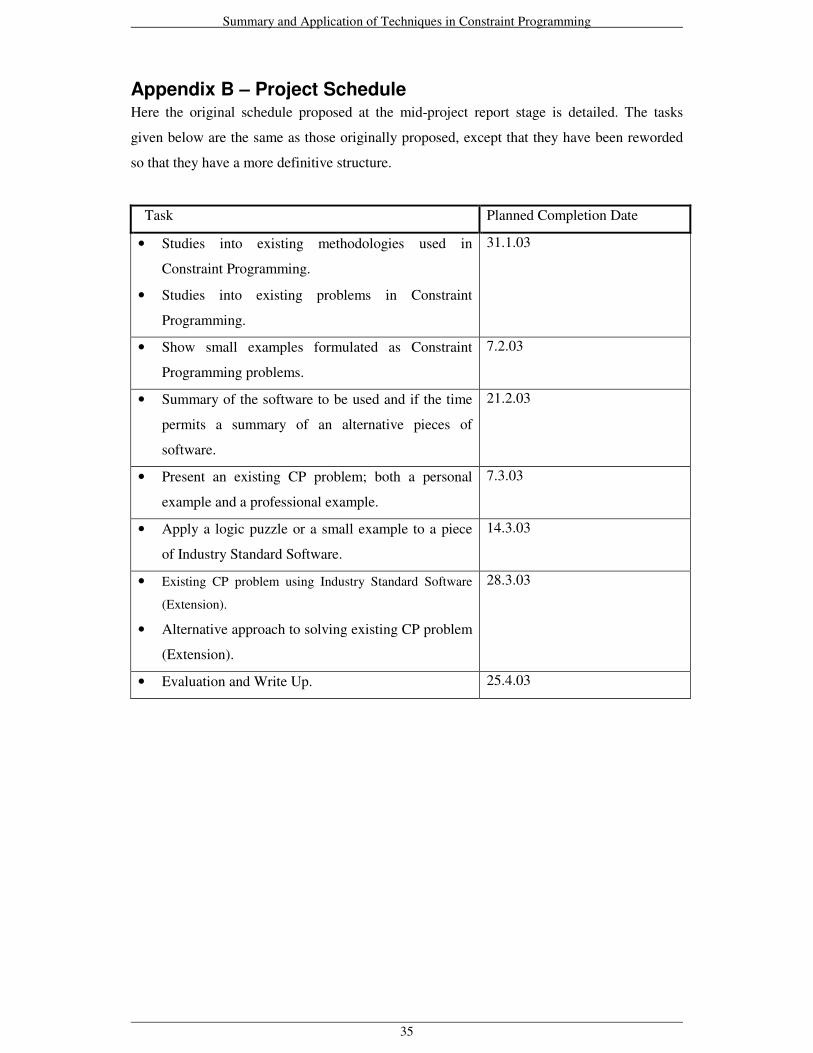
Summary and Application of Techniques in Constraint Programming
35
Appendix B – Project ScheduleHere the original schedule proposed at the mid-project report stage is detailed. The tasks
given below are the same as those originally proposed, except that they have been reworded
so that they have a more definitive structure.
Task Planned Completion Date
• Studies into existing methodologies used in
Constraint Programming.
• Studies into existing problems in Constraint
Programming.
31.1.03
• Show small examples formulated as Constraint
Programming problems.
7.2.03
• Summary of the software to be used and if the time
permits a summary of an alternative pieces of
software.
21.2.03
• Present an existing CP problem; both a personal
example and a professional example.
7.3.03
• Apply a logic puzzle or a small example to a piece
of Industry Standard Software.
14.3.03
• Existing CP problem using Industry Standard Software
(Extension).
• Alternative approach to solving existing CP problem
(Extension).
28.3.03
• Evaluation and Write Up. 25.4.03
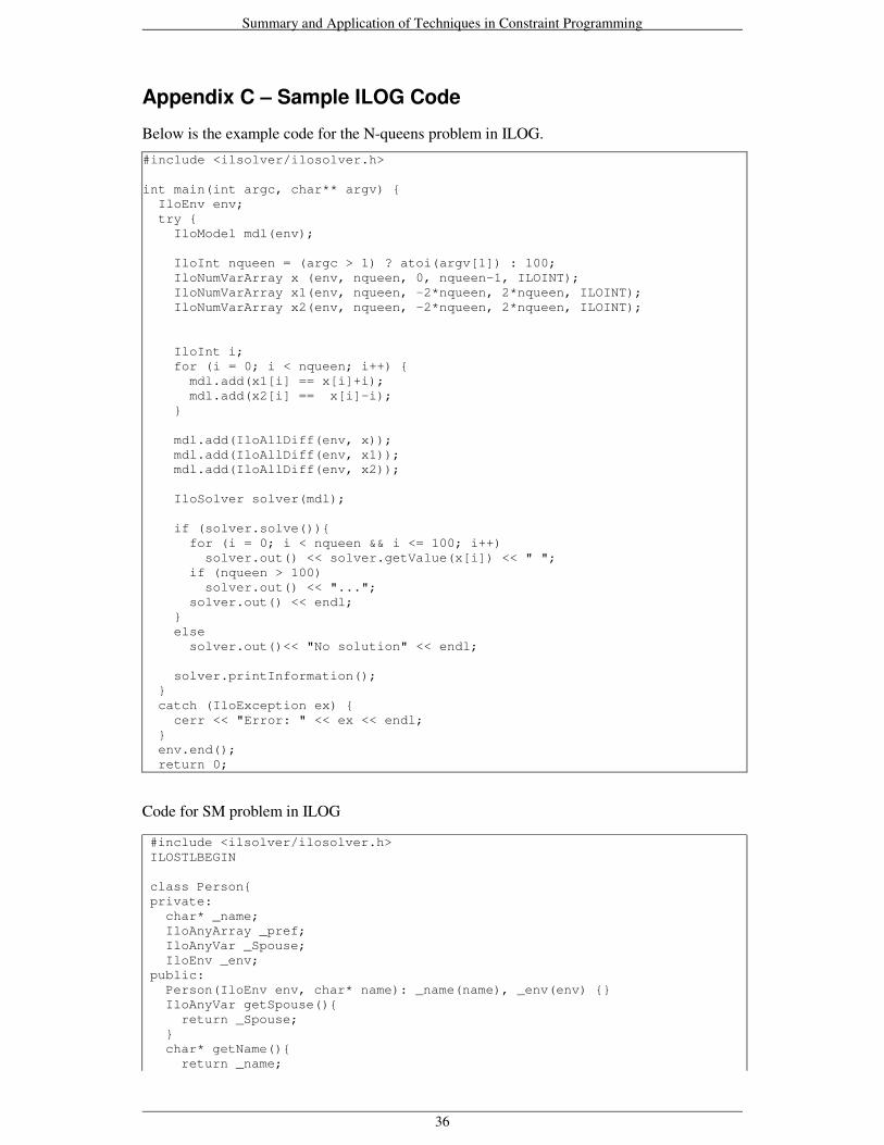
Summary and Application of Techniques in Constraint Programming
36
Appendix C – Sample ILOG Code
Below is the example code for the N-queens problem in ILOG.
#include <ilsolver/ilosolver.h>
int main(int argc, char** argv) { IloEnv env; try { IloModel mdl(env);
IloInt nqueen = (argc > 1) ? atoi(argv[1]) : 100; IloNumVarArray x (env, nqueen, 0, nqueen-1, ILOINT); IloNumVarArray x1(env, nqueen, -2*nqueen, 2*nqueen, ILOINT); IloNumVarArray x2(env, nqueen, -2*nqueen, 2*nqueen, ILOINT);
IloInt i; for (i = 0; i < nqueen; i++) { mdl.add(x1[i] == x[i]+i); mdl.add(x2[i] == x[i]-i); }
mdl.add(IloAllDiff(env, x)); mdl.add(IloAllDiff(env, x1)); mdl.add(IloAllDiff(env, x2));
IloSolver solver(mdl);
if (solver.solve()){ for (i = 0; i < nqueen && i <= 100; i++) solver.out() << solver.getValue(x[i]) << " "; if (nqueen > 100) solver.out() << "..."; solver.out() << endl; } else solver.out()<< "No solution" << endl;
solver.printInformation(); } catch (IloException ex) { cerr << "Error: " << ex << endl; } env.end(); return 0;
Code for SM problem in ILOG #include <ilsolver/ilosolver.h>ILOSTLBEGIN
class Person{private: char* _name; IloAnyArray _pref; IloAnyVar _Spouse; IloEnv _env;public: Person(IloEnv env, char* name): _name(name), _env(env) {} IloAnyVar getSpouse(){ return _Spouse; } char* getName(){ return _name;
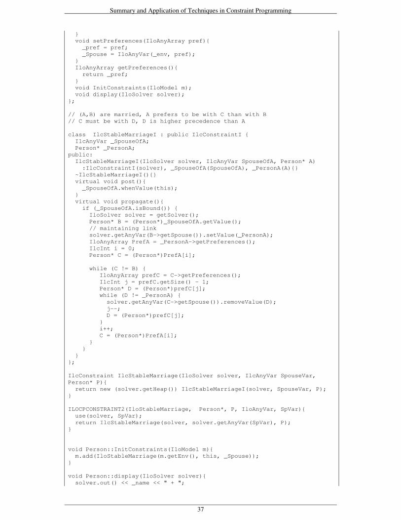
Summary and Application of Techniques in Constraint Programming
37
} void setPreferences(IloAnyArray pref){ _pref = pref; _Spouse = IloAnyVar(_env, pref); } IloAnyArray getPreferences(){ return _pref; } void InitConstraints(IloModel m); void display(IloSolver solver);};
// (A,B) are married, A prefers to be with C than with B// C must be with D, D is higher precedence than A
class IlcStableMarriageI : public IlcConstraintI { IlcAnyVar _SpouseOfA; Person* _PersonA;public: IlcStableMarriageI(IloSolver solver, IlcAnyVar SpouseOfA, Person* A) :IlcConstraintI(solver), _SpouseOfA(SpouseOfA), _PersonA(A){} ~IlcStableMarriageI(){} virtual void post(){ _SpouseOfA.whenValue(this); } virtual void propagate(){ if (_SpouseOfA.isBound()) { IloSolver solver = getSolver(); Person* B = (Person*)_SpouseOfA.getValue(); // maintaining link solver.getAnyVar(B->getSpouse()).setValue(_PersonA); IloAnyArray PrefA = _PersonA->getPreferences(); IlcInt i = 0; Person* C = (Person*)PrefA[i];
while (C != B) {IloAnyArray prefC = C->getPreferences();IlcInt j = prefC.getSize() - 1;Person* D = (Person*)prefC[j];while (D != _PersonA) { solver.getAnyVar(C->getSpouse()).removeValue(D); j--; D = (Person*)prefC[j];}i++;C = (Person*)PrefA[i];
} } }};
IlcConstraint IlcStableMarriage(IloSolver solver, IlcAnyVar SpouseVar,Person* P){ return new (solver.getHeap()) IlcStableMarriageI(solver, SpouseVar, P);}
ILOCPCONSTRAINT2(IloStableMarriage, Person*, P, IloAnyVar, SpVar){ use(solver, SpVar); return IlcStableMarriage(solver, solver.getAnyVar(SpVar), P);}
void Person::InitConstraints(IloModel m){ m.add(IloStableMarriage(m.getEnv(), this, _Spouse));}
void Person::display(IloSolver solver){ solver.out() << _name << " + ";

Summary and Application of Techniques in Constraint Programming
38
if (solver.getAnyVar(_Spouse).isBound()) solver.out() << ((Person*)(solver.getAnyValue(_Spouse)))->getName(); else solver.out() << "?" << endl; solver.out() << endl;}
int main() { IloEnv env; try { IloModel model(env); Person Richard(env, "Richard"); Person James(env, "James"); Person John(env, "John"); Person Hugh(env, "Hugh"); Person Greg(env, "Greg");
Person Helen(env, "Helen"); Person Tracy(env, "Tracy"); Person Linda(env, "Linda"); Person Sally(env, "Sally"); Person Wanda(env, "Wanda"); Richard.setPreferences(IloAnyArray(env, 5,
&Tracy,&Linda,&Wanda,&Sally,&Helen)); James.setPreferences(IloAnyArray(env, 5,
&Tracy,&Sally,&Linda,&Helen,&Wanda)); John.setPreferences(IloAnyArray(env, 5,
&Wanda,&Linda,&Tracy,&Sally,&Helen)); Hugh.setPreferences(IloAnyArray(env, 5,
&Helen,&Wanda,&Sally,&Linda,&Tracy)); Greg.setPreferences(IloAnyArray(env, 5,
&Sally,&Linda,&Tracy,&Helen,&Wanda)); Helen.setPreferences(IloAnyArray(env, 5,
&Richard,&James,&Hugh,&John,&Greg)); Tracy.setPreferences(IloAnyArray(env, 5,
&John,&Hugh,&Richard,&Greg,&James)); Linda.setPreferences(IloAnyArray(env, 5,
&Hugh,&John,&Greg,&James,&Richard)); Sally.setPreferences(IloAnyArray(env, 5,
&Richard,&Greg,&James,&Hugh,&John)); Wanda.setPreferences(IloAnyArray(env, 5,
&Greg,&James,&John,&Richard,&Hugh)); IloAnyArray MenWomen(env, 10, &Richard, &James, &John, &Hugh, &Greg,
&Helen, &Tracy, &Linda, &Sally, &Wanda);
IlcInt i; IlcInt size = MenWomen.getSize() ; for(i = 0; i < size; i++) ((Person*)MenWomen[i])->InitConstraints(model);
IloAnyVarArray SpouseArray(env, size); for (i = 0 ; i < size ; i++) { SpouseArray[i]=((Person*)MenWomen[i])->getSpouse(); } IloGoal goal = IloGenerate(env, SpouseArray, IlcChooseMinSizeAny);
IloSolver solver(model);
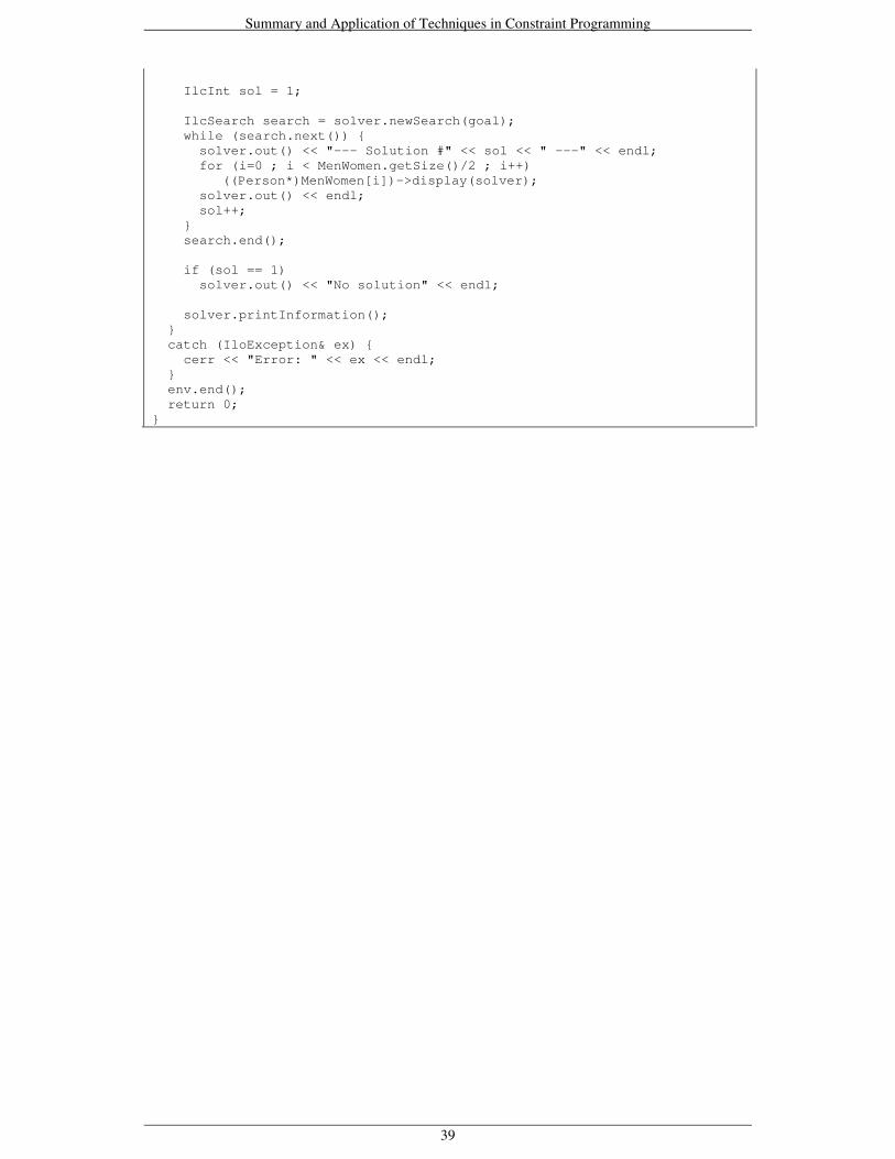
Summary and Application of Techniques in Constraint Programming
39
IlcInt sol = 1;
IlcSearch search = solver.newSearch(goal); while (search.next()) { solver.out() << "--- Solution #" << sol << " ---" << endl; for (i=0 ; i < MenWomen.getSize()/2 ; i++)
((Person*)MenWomen[i])->display(solver); solver.out() << endl; sol++; } search.end();
if (sol == 1) solver.out() << "No solution" << endl;
solver.printInformation(); } catch (IloException& ex) { cerr << "Error: " << ex << endl; } env.end(); return 0;}

Summary and Application of Techniques in Constraint Programming
40
Appendix D – University Admissions Preference Lists
Preference Lists for the Second Attempt
The preference lists for each of the ten students is given below.
S1 (C1, C2, C3)
S2 (C1, C3, C2)
S3 (C1, C2, C3)
S4 (C2, C1, C3)
S5 (C1, C3, C2)
S6 (C3, C1, C2)
S7 (C1, C3, C2)
S8 (C2, C3, C1)
S9 (C1, C3, C2)
S10 (C1, C2, C3)
The preference lists for each of the three courses is given below.
C1 (S1, S2, S3, S4, S5, S6, S7, S8, S9, S10)
C2 (S3, S4, S2, S1, S7, S8, S5, S6, S9, S10)
C3 (S1, S3, S2, S4, S5, S7, S6, S8, S10, S9)
Preference Lists for the Third Attempt
The preference lists for each of the ten students is given below.
S1 (C1, C2, C3, C4, C5, C6)
S2 (C3, C7, C10, C1, C14, C15)
S3 (C2, C4, C3, C10, C15, C1)
S4 (C8, C9, C1, C2, C3, C13)
S5 (C12, C3, C4, C8, C10, C11)
S6 (C13, C1, C4, C5, C7, C12)
S7 (C4, C5, C8, C13, C14, C15)
S8 (C3, C1, C2, C7, C8, C9)
S9 (C15, C14, C13, C12, C11, C10)
S10 (C6, C5, C1, C10, C8, C7)
The preference lists for each of the fifteen courses is given below.
C1 (S1, S2, S3, S4, S5, S6, S7, S8, S9, S10)
C2 (S3, S4, S2, S1, S7, S8, S5, S6, S9, S10)
C3 (S1, S3, S2, S4, S5, S7, S6, S8, S10, S9)
C4 (S5, S4, S1, S2, S3, S6, S8, S7, S9, S10)
C5 (S5, S4, S1, S2, S3, S6, S8, S7, S9, S10)

Summary and Application of Techniques in Constraint Programming
41
C6 (S4, S3, S2, S1, S5, S10, S9, S8, S7, S6)
C7 (S1, S7, S5, S8, S2, S4, S3, S9, S6, S10)
C8 (S3, S4, S5, S1, S2, S6, S7, S9, S8, S10)
C9 (S7, S1, S3, S5, S9, S2, S4, S6, S8, S10)
C10 (S2, S7, S8, S6, S10, S9, S1, S4, S3, S5)
C11 (S3, S5, S2, S7, S8, S4, S1, S9, S6, S10)
C12 (S4, S1, S3, S2, S6, S5, S9, S10, S8, S7)
C13 (S1, S2, S3, S4, S6, S7, S5, S10, S9, S8)
C14 (S5, S1, S7, S2, S3, S4, S6, S8, S9, S10)
C15 (S3, S2, S1, S4, S5, S6, S7, S8, S9, S10)