The Office of Financial Research (OFR) Working Paper Series allows members of the OFR staff and their coauthors to disseminate preliminary research findings in a format intended to generate discussion and critical comments. Papers in the OFR Working Paper Series are works in progress and subject to revision. Views and opinions expressed are those of the authors and do not necessarily represent official positions or policy of the OFR or Treasury. Comments and suggestions for improvements are welcome and should be directed to the authors. OFR working papers may be quoted without additional permission.

Gauging Form PF: Data Tolerances in Regulatory Reporting on Hedge Fund Risk Exposures

Mark D. Flood Office of Financial Research Mark.Flood@treasury.gov

Phillip Monin Office of Financial Research Phillip.Monin@treasury.gov

Lina Bandyopadhyay Federal Reserve Bank of Chicago lina.bandyopadhyay@chi.frb.org

15-13 | July 30, 2015

1

Gauging Form PF Data Tolerances in Regulatory Reporting on

Hedge Fund Risk Exposures

Mark D. Flood Office of Financial Research Mark.Flood@treasury.gov Phillip Monin Office of Financial Research Phillip.Monin@treasury.gov Lina Bandyopadhyay Federal Reserve Bank of Chicago lina.bandyopadhyay@chi.frb.org

July 30, 2015

ALL COMMENTS WELCOME Views and opinions expressed are those of the authors and do not necessarily represent official OFR or Treasury positions or policy. Comments are welcome as are suggestions for improvements, and should be directed to the authors. We gratefully acknowledge helpful comments from Danny Barth, Greg Feldberg, Mark Flannery, Mila Getmansky-Sherman, David Johnson, Alicia Marshall, Stathis Tompaidis, Russ Wermers, and seminar participants at the Securities and Exchange Commission, and at the May 2015 meeting of the Consortium for Systemic Risk Analytics at the Massachusetts Institute of Technology. We thank Andrew Morehead for data management support. Any remaining errors are the responsibility of the authors alone.

2

Gauging Form PF Data Tolerances in Regulatory Reporting on

Hedge Fund Risk Exposures Abstract

This paper examines the precision of the U.S. Securities and Exchange Commission’s Form PF as an instrument for measuring market risk exposures in the hedge fund industry. We introduce a novel methodology that systematically presents the measurement instrument, Form PF, with a range of simulated portfolios with observable characteristics. We assess the measurement tolerances of Form PF by examining the range of actual market risk exposures – measured directly from portfolio details – that are consistent with a given, fixed presentation on the form. We find that Form PF’s measurement tolerances are sufficiently large to allow private funds with dissimilar actual risk profiles to report similar risks to regulators. We also find that the form’s stratification by value at risk (Form PF Question 40) helps significantly to narrow the measurement tolerances.

Keywords:

Hedge funds; Form PF; data quality; risk monitoring

3

This paper examines the precision of the U.S. Securities and Exchange Commission’s (SEC) Form PF as an instrument for measuring market risk exposures in the hedge fund industry. We introduce a novel methodology that systematically presents the measurement instrument, Form PF, with a range of simulated portfolios with observable characteristics. We assess the measurement tolerances of Form PF by examining the minimum-maximum range of actual market risk exposures – measured directly from portfolio details – that are consistent with a fixed presentation of the portfolio on the form.

Every measurement framework faces the challenge of precision. We find that Form PF’s measurement tolerances are significant, and may obscure reporting funds’ actual risks. For example, the maximum expected shortfall for our factor-alpha strategy across our sample of portfolios varies from 85 to 278 percent above the median value in four versions of expected shortfall. On the other hand, we also find that the form’s stratification by value at risk (VaR), under Form PF Question 40, significantly reduces the range of possible differences between reported and actual market risk exposures. For example, the comparable results for expected shortfall in this case range (with the same ordering) from 15 to 85 percent higher than the median. This improvement in precision does not eliminate fully the potential for inaccuracies. Moreover, our results are conservative in the set of risk measures examined and portfolio strategies allowed, and thus represent a lower bound on the actual tolerances expected in more realistic portfolios. The constrained maximization methodology we present could be a useful tool in assessing Form PF or designing future regulatory risk reports.

Hedge funds are part of a broader ecosystem of investable capital that pool investors’ wealth to achieve economies of scale in portfolio management. Hedge funds can differ from other asset managers, such as mutual funds, private equity, and family offices, because SEC rules give hedge funds regulatory relief from certain terms of the Investment Company Act of 1940 (the “1940 Act”), exempting them from many investment constraints and disclosure and registration requirements while restricting their class of investors.1 This exemption from

1 Section 3(c)(1) of the 1940 Act provides regulatory relief to those private investment companies with fewer than 100 shareholders and no public offerings. Chapter 2 of the SEC’s [1992] “Protecting Investors” study highlighted the compliance costs of 1940 Act rules for certain private investment companies. The National Securities Markets Improvement Act of 1996 replaced Section 3(c)(7) of the 1940 Act with language defining “qualified purchasers,” creating a new category of regulatory relief. In June 1997, the SEC promulgated regulations implementing the new structure; see U.S. Congress [1996], SEC [1997] and Parry [2001]. The 2012 Jumpstart Our Business Startups Act (the “JOBS Act”) amended section 12(g)(1) of the Securities Exchange Act of 1934 (the “1934 Act”) to relax the

4

registration threshold for such 3(c)(7) funds – the number of investors (qualified purchasers) above which the fund would have to register publicly with the SEC – from 500 to 2000 individuals. Funds operating under the 3(c)(1) rules – i.e., not relying on qualified purchasers – are still subject to the 100-shareholder limit; see Greene [2013].

scrutiny has helped hedge funds to implement flexible and sophisticated portfolio strategies. The crisis of Long-Term Capital Management L.P. (LTCM) in 1998 revealed that financial troubles at hedge funds could have systemic implications. The financial crisis of 2007-09, which included a significant disruption to quant funds as a significant foreshock in August 2007 (see Khandani and Lo [2011]), reinvigorated these concerns. In the wake of the crisis Congress mandated enhanced regulatory reporting on private funds, including hedge funds, with the twin goals of investor protection and systemic risk assessment. The mandate was part of much broader financial reforms under the Dodd-Frank Wall Street Reform and Consumer Protection Act (Dodd-Frank Act); see U.S. Congress [2010].2

Form PF is the primary regulatory implementation of that mandate. Form PF is still quite new, and regulators – the SEC and the Commodity Futures Trading Commission (CFTC) – are required by law to hold the reported numbers closely confidential. As a result, research on Form PF is relatively sparse. However, the form itself is public information, and industry commentary has accumulated as funds have worked to comply with the new reporting requirement. The methodology discussed here is notable in that it does not require any confidential information, such as actual Form PF reports.3 In principle, anyone with access to the form and its instructions can repeat or extend the analysis.

The remainder of the paper proceeds in four sections. Section 1 discusses the debates on the possibilities for hedge funds to create systemic hazards, and policy responses that culminated in the reporting of exposures on Form PF. Some of these vulnerabilities point to actual crises, such as the LTCM failure, while others are informed conjectures. Section 2 discusses the structure of Form PF itself, and how it attempts to measure market risk exposures. Section 3 introduces the details of our simulation methodology and Section 4 presents the results and conclusions.

2 Khandani and Lo [2011] discuss the 2007 quant fund disruption. For analyses of the role of hedge funds, see House Committee on Financial Services [2007], Lo [2008], Boyson et al. [2010], Gropp [2014], Mitchell and Pulvino [2012], Dixon et al. [2012, ch. 4], FCIC [2011], Dudley and Nimalendran [2011], and Sialm, et al. [2013]. Notably, Title IV of the Dodd-Frank Act, which mandates Form PF, mentions “systemic risk” in 10 separate locations, including once in the title of Section 404. Section 404 also refers to “protection of investors” in six distinct places. 3 Section 2.3 below presents some summary statistics of actual Form PF filings as of year-end 2013.

5

1. The challenges of risk reporting for hedge funds

Section 404 of the Dodd-Frank Act requires hedge funds to maintain detailed records on their portfolio exposures, and mandates the SEC to require funds to report on those records for investor protection and systemic risk assessment.4 In November 2011, the CFTC and SEC issued a joint rulemaking that defined the specific reporting requirements that implement this mandate.5 Form PF is the centerpiece of this implementation. As a practical matter, we restrict attention in this paper to hedge funds with equity investment strategies that would be required by the SEC to file Form PF.

Given a goal of assessing performance and market risk exposures in hedge funds, we consider the empirical accuracy of Form PF as a measurement device. SEC Chair Mary Jo White [2014] highlighted some of the challenges of risk measurement for asset managers generally, noting “[w]hile funds and advisers currently report significant information about their portfolios and operations to the Commission, these reporting obligations have not, in my view, adequately kept pace with emerging products and strategies being used in the asset management industry.” Capturing historical performance and future risks is complicated, in part because hedge funds may have highly nonlinear and nonmonotonic exposures to underlying risk factors. The challenges go beyond the basic statistical artifacts in performance time series, such as survivorship bias (e.g., Amin and Kat [2003]), style drift (Wermers [2012]), or serial correlation due to illiquidity (Getmansky et al. [2004]).

One important class of mismeasurement is the intentional disguising of actual risk and performance. The incentives for performance manipulation are well-known (and not limited to hedge funds). Lo [2001], for example, offers a simple textbook example of a “Russian roulette” strategy that pays the manager handsome performance fees (in expectation), while guaranteeing eventual ruin by selling deep out-of-the-money puts on a stock market index. On the other hand, Lan, Wang and Yang [2013] provide empirical evidence that fund managers endogenously tend to adopt more risk averse strategies to prolong survival as losses gradually erode capital. Theoretical results, such as those of Hodder and Jackwerth [2007] or Goetzmann et al. [2003], show that risk-taking incentives can become quite complex when more realistic features of compensation contracts are included.

4 In particular, the Dodd-Frank Act’s Section 404 amends Section 204 of the Investment Advisers Act of 1940 by inserting a new subsection 204(b) on “Records and Reports of Private Funds.” See Dodd-Frank Act [2010], Section 404. 5 See CFTC-SEC [2011].

6

Goetzmann et al. [2007] suggest a class of manipulation-proof performance measures (MPPMs) that improve on standard industry benchmarks, such as a simple Sharpe ratio, but even MPPMs have two fundamental limitations. First, as Foster and Young [2010] show, even if the performance metric itself is manipulation-proof, compensation schemes can still be gamed. Ultimately, only transparency into detailed portfolio holdings can defeat a manager who is determined to deceive.

Second, performance benchmarks are necessarily backward-looking measures, which do not account for the possibility of fundamental changes in the portfolio allocation over time. Temporary window dressing of portfolios is a well-known tactic to hide risky positions or enhance reported performance (e.g., Sias [2007]; Sias and Starks [1997]). Others have investigated possible window dressing for various types of investment portfolios, including pension funds (e.g., Lakonishok, et al. [1991]), money funds (Griffiths and Winters [2005]), bond funds (Ortiz et al. [2012]), and mutual funds (Agarwal et al. [2014]). The regulators were clearly aware of the potential for window dressing in designing Form PF, stating that “certain data in the Form, while filed with the Commissions on an annual or quarterly basis, must be reported on a monthly basis to provide sufficiently granular data to allow FSOC [Financial Stability Oversight Council] to better identify trends and to mitigate ‘window dressing’;” see CFTC-SEC [2011, p. 71151]. It is an empirical question whether monthly observations are adequate to discourage this behavior fully.

Most studies of window dressing focus on the incentives for managers to deceive investors, but the same portfolio management tactics could work to hide market risk exposures from regulators. Munyan [2014] shows participants in the triparty repo market systematically but temporarily hide billions of dollars in repo borrowing at the end of each calendar quarter, presumably to disguise their true risk profiles. In other markets, there is evidence that window dressing occurs, but at different frequencies, so that reducing measurement intervals can help detect the tactic. For example, Elton et al. [2010] find that, unlike repo markets, equity mutual funds tend to engage in annual – but not more frequent – window dressing. Therefore, quarterly reporting for these funds should typically be adequate to reveal the activity. Nonetheless, monthly observations are valuable in analyzing a range of other tactics, such as momentum trading and tournament behavior.

For hedge funds, there are indications of window dressing at daily, monthly, and annual frequencies. Patton and Ramadorai [2013] use a factor model to infer daily time series of

7

hedge fund risk exposures, and find significant day-of-month seasonalities consistent with certain forms of window dressing. Bollen and Pool [2009] find that small positive monthly returns far exceed small losses, and this disparity tends to vanish in the quarter just preceding an audit. Moreover, this appears not to be simply an artifact of regression to the mean. Rather, there is a pattern in bimonthly returns, such that small gains in the first month tend to be reversed by small losses in the second, suggesting that many hedge fund managers engage in window dressing. Agarwal et al. [2011] find a year-end spike in monthly reported performance for hedge funds, and that this anomaly tends to increase with incentive fees and opportunities for returns management. They conclude that hedge fund managers tend to inflate returns opportunistically to manipulate their compensation.

2. Form PF as a measurement instrument

2.1. Private fund reporting under the Dodd-Frank Act

Title IV of the Dodd-Frank Act eliminates the long-standing exemption from registration for private investment advisers (Section 403) and clarifies the recordkeeping and reporting requirements for covered investment advisers (Section 404). Specifically, any adviser (except those specifically exempted under Sections 407-409) of a private fund must now register with the SEC.6 Registered advisers must maintain records regarding the fund’s activities and file reports with the SEC “as necessary and appropriate in the public interest and for the protection of investors, or for the assessment of the systemic risk.” Records must include information on assets under management, use of leverage, counterparty credit risk exposure, trading and investment positions, valuation policies and practices, types of assets, side arrangements or side letters, and trading practices. As noted above, a central goal of the new registration mandate is to provide the necessary information to evaluate the systemic risk of the covered funds.

In November 2011, the CFTC and SEC (CFTC-SEC [2011]) announced the introduction of Form PF in a joint rulemaking that implemented the statutory provisions mandated by Title

6 Title IV has 19 Sections in all. Sections 403 and 404 are the most significant; the others are largely technical in nature. Section 407 defines registration exemptions for venture capital funds. Section 408 establishes an exemption from registration for advisers of small funds – those with assets under management (AUM) less than $150 million. Section 409 defines registration exemptions for family offices.

8

IV. Formally, it applied registration, recordkeeping, and reporting requirements to the “private fund advisers” (i.e., portfolio managers) for covered funds.7 The SEC [2014a] later clarified that “a hedge fund is defined generally to be any private fund that has the ability to pay a performance fee to its adviser, borrow in excess of a certain amount, or sell assets short.”8 This distinction only affects the reporting requirements on Form PF; hedge funds do not face special regulation relative to other private funds; see also PWC [2011, p. 4]. Private fund advisers exceeding $1.5 billion in assets under management (AUM) are classified as large private fund advisers and must file Form PF quarterly and provide various data for each of the three months in the reporting period. All other private fund advisers must file annually, and only gross and net performance data are requested at a monthly frequency.

While the SEC supervises hedge funds, the CFTC, under its Regulation 4.27, maintains related Forms CTA-PR and CPO-PQR for commodity trading advisers (CTAs) and commodity pool operators (CPOs), respectively. CTAs and CPOs advising private funds and registered as investment advisers with the SEC must file Form PF. CFTC-registered entities qualifying as both hedge funds and CPOs may submit Form PF in lieu of CPO-PQR. The information reported through the various forms is designed to be complementary, not duplicative. For dual-registered CPOs and CTAs, filing Form PF is deemed a filing with both the SEC and CFTC.9 Because our analysis of measurement tolerances involves equity hedge funds, we focus solely on Form PF in the subsequent analysis.

The SEC separately collects certain basic information on private fund advisers through Form ADV, and certain details of institutional investor holdings on Form 13F. In both cases, however, the information is not well suited to assessing funds’ risks in general or systemic risks in particular. Form ADV includes little information on performance, leverage, or risks of managed funds. Form 13F has limited scope, covering only U.S. holdings for a specific list of securities (SEC [2014b]); it also omits short positions and derivatives. On the other

7 Advisers with AUM under $100 million (or an amount specified by state authorities) must typically register with the authorities of the state of their principal place of business, rather than with the SEC. 8 For additional nuance, see the SEC [2013] Investor Bulletin on hedge funds. 9 However, any private fund adviser that is also registered as a CPO or CTA with the CFTC must file Schedule A of Form CPO-PQR (for CPOs) or Schedule A of Form CTA-PR (for CTAs).

9

hand, information reported on Forms ADV and 13F is publicly available, while information reported on Forms PF, CPO-PQR and CTA-PR are held confidentially by the regulators.10

Sec. Information about To be completed by Ques. Reg.

1a The filer and related persons

All Form PF filers 1–4 SEC & CFTC

1b Private funds advised All Form PF filers 5–17 SEC & CFTC

1c Hedge funds advised All Form PF filers that advise hedge funds

18–25 SEC & CFTC

2a Aggregates on hedge funds advised

Large private fund advisers only 26–28 SEC & CFTC

2b Qualifying hedge funds advised

Large private fund advisers only 29–50 SEC & CFTC

3 Liquidity funds advised Large private fund advisers only 51–64 SEC only

4 Private equity funds advised

Large private fund advisers only 65–79 SEC only

5 Temporary hardship exemption request

Private fund advisers requesting exemption

--- SEC only

Exhibit 1: Sections of Form PF Source: SEC [2011a]

2.2. The structure of Form PF

As outlined in Exhibit 1, Form PF has five major sections, with Sections 1 and 2 subdividing into subsections. Sections 1–4 contain a series of sequentially numbered questions, 79 in all. Section 5 is a request for additional time to file; Form PF reports are due within 60 days of quarter end for large hedge funds, and within 120 days of the fiscal year end for annual filers. All Form PF filers must file Section 1. Section 1a consists mostly of basic census data, including identifying information, such as the large trader ID, linking the Form PF filing to Form ADV. Only large private fund advisers (the “large” threshold for hedge funds is $1.5 10 The OFR has access to Form PF data through a cooperative agreement with the SEC, subject to the same confidentiality rules. See, for example, OFR [2014, 114-115].

10

billion in AUM) must report the more detailed information in Sections 2–4 of Form PF.11 Section 3 covers liquidity funds; these advisers report only to the SEC. Section 4 covers private equity funds; these advisers also report only to the SEC.

Form PF is a complicated report, and its intricacies are a source of possible measurement errors and ambiguities. The following list highlights some of the form’s nuances:

• In general, for derivatives (other than options), “value” on Form PF means gross notional value. For options, it is the delta-adjusted notional value; for interest-rate derivatives, it is the 10-year bond equivalent; see SEC [2015]. For all other investments, or the reporting fund’s borrowings, “value” is market value (or fair value if market prices are lacking).

• Question 3 collects the aggregate “regulatory” (i.e., gross) and net AUM on all the adviser’s private funds, by type of fund (hedge fund, private equity, etc.).

• Question 4 allows the filer to comment on any assumptions (including, for example, specifics of fund conventions, valuation and accounting) made in responding to any question on the form.

• Section 1b collects information on each fund’s gross and net assets and the aggregate notional value of derivative positions. Gross assets are equivalent to regulatory assets under management (RAUM).12

• The breakdown of assets and liabilities in Section 1b uses the fair value taxonomy established under U.S. generally accepted accounting principles (GAAP).

• Question 15 collects the percentage concentration of the funds’ large investor base, defined by the five largest equity stakes. Question 16 collects concentrations for all investors, by investor type (broker-dealers, U.S. persons, etc.)

• Question 21 is a simple breakdown of the use of high-frequency trading.

• Questions 22 and 23 request the identities of and exposures to the fund’s five largest counterparties, for both incoming and outgoing net credit exposures.13

• Question 24 is a breakdown by trading and clearing mechanism.

• Section 2 collects a detailed breakdown by product type, turnover, and domicile.

• Question 30 gives advisers discretion to report weighted-average tenor or 10-year bond equivalents in lieu of duration.

11 More specifically, “large” private funds are hedge funds with at least $1.5 billion in assets under management, private equity funds with at least $2 billion in assets under management, or liquidity funds with at least $1 billion assets under management attributable to liquidity funds and registered money market funds; see PWC [2011, p. 5]. 12 Form ADV defines RAUM. See SEC [2011b], Part 1A, instruction 5.b. 13 This is roughly in line with Duffie’s [2014] “10-by-10-by-10” proposal.

11

In addition to the potential for window dressing (see Section 1 above), there are several data issues that make analysis of the private funds on a standardized basis challenging. In some cases, such as fair valuation methodologies, filers have discretion in their choice of approaches. Form PF is lengthy and complex, and some definitions are not perfectly aligned with industry norms, so there is the potential for filer errors or misinterpretations. There is no certification requirement for Form PF filings.14 As always with risk data, separating data quality issues (inaccuracies) from genuine (accurate) outliers is a challenge.

Fund portfolios comprise large numbers of diverse investment positions. While many of these positions individually are relatively simple in structure, such as the individual equities we consider, hedge funds ordinarily combine long and short positions in various securities and related derivatives. The net market risk exposures in a typical hedge fund portfolio can therefore include one or more significant basis risk exposure(s). These exposures can be highly nonlinear and nonmonotonic functions of the fundamental risk factors affecting position values. Leverage will typically magnify small impacts, including any measurement errors, compounding the challenge of assessing the final risk profile of a portfolio.

One can view risk assessment generally as a process of approximating a function that describes the portfolio value’s response to fluctuations in a set of underlying risk factors. Broadly, there are two approaches, differing in whether one collects the inputs or the outputs of the portfolio valuation calculations. Starting with the inputs, one can capture the detailed terms and conditions that describe the contracts composing the portfolio, and use formal valuation models to revalue the portfolio under the scenarios of interest. Alternately, one can delegate the scenario valuation to experts and/or specialized software, and capture only the “bottom-line,” scenario-specific valuation outcomes.15 The former approach offers analytical flexibility, but also entails a significant burden of software maintenance, data modeling and data management. The latter approach relinquishes much of this burden, but also much of the flexibility of customized risk and valuation analysis.

14 Earlier proposals had suggested that filings should be certified as accurate under penalty of perjury; see PWC [2011, p. 3]. 15 Of course, there is also a rich middle ground between these two stylized extremes, of emulation techniques and mark-to-market and mark-to-model approximations. For instance, much of the academic literature on hedge fund risks must make do with publicly reported hedge fund returns; see, for example, Adrian [2007], Adrian et al. [2013], Fung and Hsieh [2001, 2004], Li et al. [2013], Lo [2001], López de Prado and Peijan [2004], and Patton and Ramadorai [2013]. Portfolio aggregation is another possible variable. For example, one might divide the problem into sub-portfolios and use a mix of different approaches. Re-aggregating the separately calculated risk measures is itself a challenge.

12

In designing Form PF, the SEC and CFTC pursued the latter approach. This obviates the need for regulators to maintain sophisticated portfolio analytics and data models that would need to keep up with the industry’s pace of financial innovation. However, it can also entail significant approximation errors in identifying the portfolio’s factor-response function. In principle, one can approximate any continuous function to arbitrary accuracy by sampling it at a sufficiently large number of well distributed points. This is the essence of Monte Carlo integration, for example. However, an arbitrary hedge fund portfolio can exist in a very high dimensional factor space, and the regulators face significant constraints on the compliance burden they are allowed to impose.16

The result is a restrictive budget for reported values to sample the contours of the portfolio’s risk profile. Given a binding analytical constraint, regulators must trade off specialized risk calculations against the compliance burden those measures impose, and the possibility that carefully tailored calculations might be made obsolete by financial innovation. As we show below, these trade-offs are real. A Form PF filing defines a vector of risk statistics that describe the portfolio, but there can be many other portfolios with these same statistics

2.3. Market aggregates

The details of private funds reported on Form PF (together with information on Forms ADV, 13F, CPO-PQR and CTA-PR) give regulators a baseline depiction of potential systemic risk across the entire private fund industry. The following exhibits, based on Form PF filings, provide a glimpse into the state of the private-fund sector as of December 31, 2013.17 One takeaway from this overview is that it is reasonable to focus our example on listed equity portfolios, as we do in the next section.

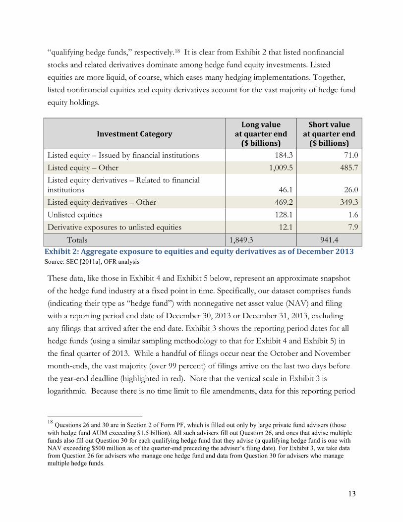
Exhibit 2 lists some high-level aggregates for reported equity holdings of hedge funds as of December 2013, based on Form PF Questions 26 and 30, which report (for large fund advisers) the notional values of asset exposures in various categories for “hedge funds” and

16 Under the Paperwork Reduction Act, the Office of Management and Budget (OMB) assesses the compliance burden associated with regulatory data collections. For Form PF, the OMB estimated a burden of 52.88 person-hours to file the form, per investment adviser, per quarter (or year, as appropriate). As a point of comparison, the estimated burden for bank Call Reports is similar, at 48.3 hours per respondent; see Federal Financial Institutions Examination Council [2014, p. 1]. 17 See SEC [2014a] for a related summary of Form PF data.

13

“qualifying hedge funds,” respectively.18 It is clear from Exhibit 2 that listed nonfinancial stocks and related derivatives dominate among hedge fund equity investments. Listed equities are more liquid, of course, which eases many hedging implementations. Together, listed nonfinancial equities and equity derivatives account for the vast majority of hedge fund equity holdings.

Investment Category Long value

at quarter end ($ billions)

Short value at quarter end

($ billions) Listed equity – Issued by financial institutions 184.3 71.0 Listed equity – Other 1,009.5 485.7 Listed equity derivatives – Related to financial institutions 46.1 26.0 Listed equity derivatives – Other 469.2 349.3 Unlisted equities 128.1 1.6 Derivative exposures to unlisted equities 12.1 7.9 Totals 1,849.3 941.4

Exhibit 2: Aggregate exposure to equities and equity derivatives as of December 2013 Source: SEC [2011a], OFR analysis

These data, like those in Exhibit 4 and Exhibit 5 below, represent an approximate snapshot of the hedge fund industry at a fixed point in time. Specifically, our dataset comprises funds (indicating their type as “hedge fund”) with nonnegative net asset value (NAV) and filing with a reporting period end date of December 30, 2013 or December 31, 2013, excluding any filings that arrived after the end date. Exhibit 3 shows the reporting period dates for all hedge funds (using a similar sampling methodology to that for Exhibit 4 and Exhibit 5) in the final quarter of 2013. While a handful of filings occur near the October and November month-ends, the vast majority (over 99 percent) of filings arrive on the last two days before the year-end deadline (highlighted in red). Note that the vertical scale in Exhibit 3 is logarithmic. Because there is no time limit to file amendments, data for this reporting period

18 Questions 26 and 30 are in Section 2 of Form PF, which is filled out only by large private fund advisers (those with hedge fund AUM exceeding $1.5 billion). All such advisers fill out Question 26, and ones that advise multiple funds also fill out Question 30 for each qualifying hedge fund that they advise (a qualifying hedge fund is one with NAV exceeding $500 million as of the quarter-end preceding the adviser’s filing date). For Exhibit 3, we take data from Question 26 for advisers who manage one hedge fund and data from Question 30 for advisers who manage multiple hedge funds.

14

are subject to change following material revisions. In Exhibit 4 and Exhibit 5, we focus only on filings from December 30 and 31, 2013.

Exhibit 3: Number of Form PF filings by date Source: SEC [2011a], OFR analysis

Exhibit 4 shows a breakdown of the aggregate assets under management (AUM) proportionally by fund strategy. Exhibit 5 is a tabular representation of the same data. For each adviser with a filing as of December 31, 2013, Exhibit 5 scales the NAV reported on Form PF Question 9 by the portfolio weight allocated to a particular strategy, as reported on Form PF Question 20. In many cases, the “% of NAV” reported on Question 20 exceeds 100 percent due to leverage. These two questions are required for all hedge fund advisers, so the table is a comprehensive snapshot of the industry. In particular, this aggregate includes non-qualifying funds, which do not complete Form PF Questions 26 or 30. The data show that the various equity strategies represent about one-third of industry AUM. The global macro, relative value sovereign debt, and long/short credit strategies also stand out. Furthermore, about one-fifth of hedge fund industry AUM is invested in funds that self-identify their strategy simply as “Other.” The magnitude of this miscellaneous category highlights the challenges of categorizing hedge fund strategies.

Exhibit 5 reveals that the aggregate AUM in the hedge fund industry as of December 2013 was about $4.1 trillion, in sharp contrast with the approximately $2.6 trillion industry aggregate AUM estimated from public sources as of that date; see the FSOC [2014a, p. 85]. The difference reflects: (a) primarily the incorporation of leverage in Exhibit 5, while the FSOC [2014a] reports net asset values; and (b) secondarily the fact that Exhibit 5 uses

11 11

36

1

201

5887

1

10

100

1000

10000

Oct 31 Nov 29 Nov 30 Dec 13 Dec 30 Dec 31

Num

ber o

f fili

ngs

(log)

Reporting Date

15

comprehensive Form PF data, while FSOC [2014a] uses data hedge funds report voluntarily to an external data aggregator.

Exhibit 4: Aggregate hedge fund AUM as of December 2013, by fund strategy Source: SEC [2011a], OFR analysis

This suggests that, as of December 2013, hedge funds representing about one-third of industry AUM did not voluntarily report their data. The total in Exhibit 5 also contrasts with the aggregate RAUM of $5,006 billion that SEC [2014a] reports for the hedge fund industry as of May, 2014. This difference may be attributable to: (a) the difference in reporting dates; (b) the possible presence of fund-of-funds reports in the SEC total; and (c) the fact that RAUM reports gross asset values, while Exhibit 5 calculates AUM by scaling reported net asset value by the reported percentage allocated to each strategy. These allocations may exceed 100 percent due to leverage. These examples highlight the challenges in accurately

Credit, Asset Based Lending

Credit, Long/Short

Equity, Long Bias

Equity, Long/Short

Equity, Market Neutral

Equity, Short Bias

Event Driven, Distressed/

Restructuring

Event Driven, Equity Special

Situations

Event Driven, Risk Arbitrage/Merger

Arbitrage Investment in other funds

Macro, Active Trading

Macro, Commodity

Macro, Currency

Macro, Global Macro

Managed Futures/CTA, Fundamental

Managed Futures/CTA, Quantitative

Other

Relative Value, Fixed Income Asset Backed

Relative Value, Fixed Income Convertible Arbitrage

Relative Value, Fixed Income

Corporate Relative Value, Fixed Income

Sovereign

Relative Value, Volatility Arbitrage

16

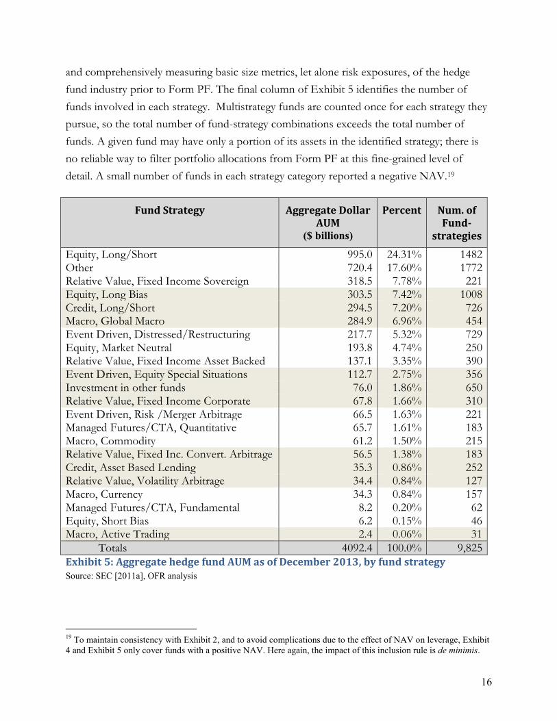
and comprehensively measuring basic size metrics, let alone risk exposures, of the hedge fund industry prior to Form PF. The final column of Exhibit 5 identifies the number of funds involved in each strategy. Multistrategy funds are counted once for each strategy they pursue, so the total number of fund-strategy combinations exceeds the total number of funds. A given fund may have only a portion of its assets in the identified strategy; there is no reliable way to filter portfolio allocations from Form PF at this fine-grained level of detail. A small number of funds in each strategy category reported a negative NAV.19

Fund Strategy Aggregate Dollar AUM

($ billions)

Percent Num. of Fund-

strategies

Equity, Long/Short 995.0 24.31% 1482 Other 720.4 17.60% 1772 Relative Value, Fixed Income Sovereign 318.5 7.78% 221 Equity, Long Bias 303.5 7.42% 1008 Credit, Long/Short 294.5 7.20% 726 Macro, Global Macro 284.9 6.96% 454 Event Driven, Distressed/Restructuring 217.7 5.32% 729 Equity, Market Neutral 193.8 4.74% 250 Relative Value, Fixed Income Asset Backed 137.1 3.35% 390 Event Driven, Equity Special Situations 112.7 2.75% 356 Investment in other funds 76.0 1.86% 650 Relative Value, Fixed Income Corporate 67.8 1.66% 310 Event Driven, Risk /Merger Arbitrage 66.5 1.63% 221 Managed Futures/CTA, Quantitative 65.7 1.61% 183 Macro, Commodity 61.2 1.50% 215 Relative Value, Fixed Inc. Convert. Arbitrage 56.5 1.38% 183 Credit, Asset Based Lending 35.3 0.86% 252 Relative Value, Volatility Arbitrage 34.4 0.84% 127 Macro, Currency 34.3 0.84% 157 Managed Futures/CTA, Fundamental 8.2 0.20% 62 Equity, Short Bias 6.2 0.15% 46 Macro, Active Trading 2.4 0.06% 31 Totals 4092.4 100.0% 9,825 Exhibit 5: Aggregate hedge fund AUM as of December 2013, by fund strategy Source: SEC [2011a], OFR analysis

19 To maintain consistency with Exhibit 2, and to avoid complications due to the effect of NAV on leverage, Exhibit 4 and Exhibit 5 only cover funds with a positive NAV. Here again, the impact of this inclusion rule is de minimis.

17

3. Our approach

3.1. Risk maximization subject to reporting and strategy constraints

Our basic approach involves constrained maximization of a hedge fund’s portfolio risk exposures. The assessment of uncertainty in measurement typically assumes that there is some underlying true value, R*, for the measurand, and that the measurement process

produces a noisy estimate of that true value (JCGM/WG1, 2008): 𝑅𝑅� = 𝑅𝑅∗ + 𝜀𝜀̃. In the simplest case, the measurand is univariate and fixed, and the distribution of the measurement error, 𝜀𝜀̃, can be established by repeated experimental observation. In contrast, the question of measurement error for hedge fund portfolio risk faces two additional challenges: (1) portfolio risk is multidimensional (volatility, expected shortfall, skewness, etc.); and (2) the official measurement process, defined by Form PF, is fixed. Given this, we address the following question: Treating a given Form PF filing as a vector-valued constraint, what is the maximum risk a portfolio can exhibit without altering the reported numbers? That is, we fix

an official measurement under Form PF, 𝑅𝑅�, and examine the range of possible deviations, 𝛿𝛿,

for a set of standard (but unofficial) portfolio risk measures, 𝑅𝑅�𝑖𝑖 , that are consistent with the

fixed official presentation: 𝑅𝑅�𝑖𝑖 = 𝑅𝑅�𝑖𝑖 + 𝛿𝛿𝑖𝑖 . Under perfect precision, 𝛿𝛿 would be zero. In most cases (VaR is the notable exception), our portfolio risk measures do not appear explicitly on

Form PF, so that 𝑅𝑅�𝑖𝑖 is not directly observable. However, because 𝑅𝑅� is fixed, even if

unobserved, the dispersion of 𝑅𝑅�𝑖𝑖 directly quantifies the measurement uncertainty, 𝛿𝛿𝑖𝑖.

We work with a range of industry-standard risk measures and two basic quantitative approaches to portfolio formation, namely a market-neutral factor-alpha screen and a market-neutral momentum strategy. There are two main reasons to expect our results to represent a lower bound on the true range of risk maxima available in a more general setting. First, to focus the discussion on Form PF rather than on the intricacies of portfolio formation and hedging, we simplify the optimization space by working with listed equities only (i.e., no options or other derivatives) and fixed leverage. By thus limiting the portfolio strategy space, we are eliminating from consideration certain exposures, such as out-of-the-money options, that might increase the maximum risk. Second, we examine only risks arising from the investment portfolio as an isolated pool of assets. We do not consider other

18

hazards – for example, those arising from the institutional context, such as redemption risk or operational risk – that might further increase the maximum.20

We examine the potential for Form PF to fail to convey the critical information needed by regulators and policymakers in assessing hedge funds’ risk profiles. Our approach is to show that even simple strategies underlying equivalent Form PF filings can have a wide spectrum of market risk associated to them. To underscore the fundamental nature of this issue with Form PF, and to stress that such problems are evident even in strategies using the most well understood and fundamental assets, we follow a simple approach using quantitatively implemented equities-based strategies. Each strategy we use provides a recipe for forming realistic portfolios of stocks that have equivalent representations on Form PF but differential risk characteristics.

3.2. Quantitative strategies and risk measures

We consider two simple quantitative equities-based strategies, each of which is a long/short market-neutral equities strategy designed to be realistic but also easily and systematically implementable using exclusively historical equities data. We do not incorporate personal or analyst views on the potential future performance of the stock, since the aim is to remove the human element altogether. We focus on stock screens and factor-neutral methods. We focus on these market-neutral long/short strategies because they are transparent to implement mechanically, because they are strategies that are available to hedge funds but not to traditional 1940 Act mutual funds, and because they are strategies that are beta-neutral, which means that they should be immunized against market moves and therefore might not be considered very risky.21

The first strategy screens stocks based on their alphas from the Carhart [1997] four factor model, which extends the canonical Fama and French [1992; 1993] three factor model to include a momentum risk factor.22 In practice, many hedge funds also sort on industry or sector factors, but these would be a superfluous complication for our exercise. The strategy

20 The Financial Stability Oversight Council’s [2014b] recent request for comment on risks in the asset management industry covers a range of risks beyond the market risks that dominate the analysis here. 21 Traditional mutual funds can run 130/30 strategies, but these are not market neutral; see Lo and Patel [2008]. 22 The Fama and French [1992; 1993] factor model proposes three drivers for equity returns, namely the market factor, “small minus big” (SMB), and “high minus low” (HML). Carhart [1997] adds a fourth momentum factor to the mix.

19

is to buy a subset of stocks in the top alpha quintile and to sell a subset of stocks in the bottom quintile. The weights in each stock are determined such that the resulting portfolio is both dollar- and beta-neutral.

The second strategy is a market-neutral momentum strategy that screens stocks based on their recent historical performance. The strategy is to buy a subset of stocks that lie in the top quintile of recent performance and to sell a subset of stocks that lie in the bottom quintile. As with the factor-alpha screen, the weights in each stock are determined such that the resulting portfolio is both dollar- and beta-neutral.23 The basic motivation for this strategy appears in Jegadeesh and Titman’s [1993; 2011] work on returns momentum and the short-run performance persistence of winners and losers. The specifics of portfolio construction for each strategy are discussed below in Section 3.3.

After constructing a given portfolio, we estimate its market risk using a variety of standard risk measures. Each risk measure takes as input a time series of continuously compounded daily empirical returns for the portfolio over five years, from January 2009 through December 2013. Where appropriate, we consider risk measures over horizons that are reasonable for a portfolio of equities, namely daily and weekly horizons. We calculate value-at-risk (VaR) using two methods, two significance levels and two horizons. Daily VaR using the historical simulation approach at the 1 percent (5 percent) significance level is found by extracting the 1st (5th) percentile from the empirical returns distribution. VaR using the parametric approach assumes a normal distribution as the data generating process for the portfolio returns. Daily VaR using the parametric approach at the 1 percent (5 percent) significance level is thus found by subtracting 2.326 (1.644) times the sample standard deviation of the empirical returns from the sample mean. Daily expected shortfall at the 1 percent (5 percent) level is computed by averaging the empirical returns less than the 1 percent (5 percent) daily VaR calculated using the historical simulations approach. These risk measures are also computed at a five-trading day horizon using portfolio returns from January 2009 through December 2013 sampled at non-overlapping five-trading day intervals. All risk measures are reported as nonnegative numbers.

We also report volatility, skewness, excess kurtosis, and the Sharpe ratio according to their common definitions. Lower semi-volatility is computed as the standard deviation of the

23 Here and throughout, we use the Capital Asset Pricing Model to determine beta, with the value-weighted portfolio on all U.S.-listed stocks in Center for Research in Securities Prices (CRSP) as the proxy for the market portfolio.

20

distribution of the minimum of the returns distribution and zero. Volatility, lower semi-volatility, and the Sharpe ratio are annualized using the square root of time rule, with T=252 days. Finally, worst loss at an n-day horizon is the lowest observed return in the time series of returns sampled at nonoverlapping n-trading day intervals.

3.3. Portfolio formation

We envision a hedge fund filing Form PF on December 31, 2013. We form portfolios and compute their associated risk metrics using historical equities data available as of that date. We obtain historical equities data from the Center for Research in Securities Prices (CRSP), which we download through the Wharton Research Data Services (WRDS). We download the entire CRSP Daily Stock dataset for all observations from January 1, 2009 through December 31, 2013. Individual stock issues are identified using the PERMNO identifier in CRSP. We then restrict our dataset of stocks to U.S. common equity stocks (CRSP share code 10 or 11) that are actively traded through the entire period on the New York Stock Exchange (NYSE), American Stock Exchange (AMEX), or NASDAQ. We further restrict our set of stocks to only those that traded continuously over the entire five-year period and had an average daily volume over that period of at least 100,000 shares. We then make the appropriate adjustments for dividends, stock splits, and other distributions (using the cumulative factors in CRSP to adjust price and shares outstanding). The above procedure results in 2,466,492 stock-date observations with appropriately adjusted price and capitalization data. Finally, we focus only on large-cap stocks, which we define as those stocks in the top 40 percent of market capitalization as of December 31, 2013. The final dataset of stock data contains 986,256 stock-date observations for 784 unique stock issues. For the factor-alpha screen strategy, we download the “Fama/French 3 Factors” and the “Momentum Factor” from the French’s [2014] online data library. These data are merged with the stock data from CRSP.

We assume that the hedge fund has $500 million in initial capital deposited with its prime broker, with 90 percent of this capital deployed to form the stock portfolios and 10 percent held as a liquidity buffer to meet marks to market on the short positions; see Jacobs and Levy [1997]. The hedge fund thus uses $450 million to purchase its desired long positions. The stocks are held at the prime broker, who then arranges to borrow $450 million in stocks to be sold short. This is consistent with Federal Reserve Board Regulation T, which requires

21

that margined positions be at least 50 percent collateralized at initiation. The cash proceeds from the sale of the shorts are provided to the securities’ lenders as collateral for the borrowed shares. This $450 million in cash collateral generally earns interest, some of which then goes to the lender as a securities’ lending fee and some of which goes to the prime broker as a fee, with the rest going to the investor as the short-rebate. For simplicity, we assume that cash in the liquidity buffer and in the collateral account earn zero interest and that the securities’ lenders’ fees and primer broker’s fees are zero, so that there is no short-rebate.

Both the market-neutral factor-alpha screen and the market-neutral momentum screen belong to the class of market-neutral long/short equity strategies. For each strategy, we form 100,000 distinct portfolios that produce the same output in relevant Form PF fields (see Exhibit 6) as of December 31, 2013. Both strategies screen stocks based on a performance measure and use the results to partition the universe of stocks into five subsets based on quintiles of the performance measure. For the market-neutral factor alpha screen, we first run the Carhart 4 Factor model on each stock and then rank each stock on its respective alpha from the regression. In this case, the alpha is the performance measure used to partition the stocks. For the market-neutral momentum screen, we first rank each of the 784 stocks in our final sample of large-cap stocks based on its realized return over the trading period from January 1, 2013 through October 31, 2013. We do not consider performance in November and December of 2013 because of the well-known short-term reversal effect; see Jegadeesh [1990]. This realized return is the performance measure used to partition the stocks into quintiles.

Having partitioned the stocks, we next determine the specific set of stocks held in each of the 100,000 distinct portfolios. Each portfolio has a sub-portfolio of longs and a sub-portfolio of shorts, with $450 million worth of assets managed in each. We randomly select 25 stocks from the top quintile for our $450 million portfolio of long positions and we randomly select 20 stocks from the bottom quintile for our $450 million portfolio of short positions. The numbers of stocks in the long and short sub-portfolios are chosen arbitrarily provided they are consistent with our requirement that the position in any individual stock is at most 5 percent of the hedge fund’s capital. With $450 million invested in both the portfolio of longs and the portfolio of shorts, the combined portfolio is dollar-neutral.

22

The amount invested in each stock is determined so that the combined portfolio is also beta-neutral. This is accomplished as follows. First, we determine each stock’s beta, as measured by the Capital Asset Pricing Model using monthly returns over a period of 60 months, the value-weighted portfolio on all U.S.-listed stocks in CRSP as a proxy for the market portfolio, and the one-month Treasury bill as a proxy for the risk-free rate. The portfolio of shorts is then set to be equally-weighted, with $22.5 million of each stock sold short. The weights in the portfolio of long positions are then set so that the (absolute) dollar value of the position in each is less than $25 million and that the beta of the portfolio of longs is equal to the beta of the portfolio of shorts. This is solved for numerically. If no solution is found, the portfolio is deemed not to be a viable portfolio, in which case new sets of stocks for the long and short portfolios are sampled. With the beta of the portfolio of shorts set equal to the beta of the portfolio of longs, each viable portfolio is beta-neutral. Moreover, the position in any individual stock in a viable portfolio is at most 5 percent ($25 million) of the hedge fund’s capital.

3.4. Constrained optimization

We show that equivalent filings of Form PF can represent a wide range of actual risk as measured by a broad array of measures. Equivalent filings of Form PF are determined by equivalent answers to the relevant questions on the form. Exhibit 6 reports the relevant fields in Form PF that we constrain to be the same for each viable portfolio.

Question 35 inquires as to the concentration of the fund’s portfolio in its constituent assets by requiring the fund to report all positions in its portfolio that exceed 5 percent of its net asset value. Our portfolio-construction methodology does not allow the assets in a viable portfolio to exceed 5 percent of the fund’s NAV, and therefore Question 35 is not applicable. Question 42 inquires as to the fund’s estimate on its NAV of various single-factor stress tests. Since each viable portfolio is beta-neutral, each viable portfolio reports zero effect from changes in equity prices. Question 43 asks for borrowing information, including types of creditors and collateral used to secure financing. In general, the cash proceeds from the short sales are posted with the lenders of the securities, which could include the prime broker as well as other stock lenders. Since it is immaterial to our objective, we have made the simplifying assumption that all of the shares for the shorts come solely from the prime broker’s inventory. Questions 40–42 are crucial, because these

23

elements directly address the market risk exposures of the portfolio. By pinning down these risk measures, Form PF should also constrain the possible values for a range of correlated risk measures. The extent to which this occurs is an empirical question. The issue is especially relevant for Question 40, value-at-risk, because VaR is one of the canonical risk measures we calculate. There are numerous “standard” definitions of VaR, which are known to correlate imperfectly. Form PF gives advisers discretion to choose a version appropriate to their portfolios.

Form PF question Description Value

8 Gross asset value $950 million 9 Net asset value $500 million

12(a) Dollar amount of total borrowings $450 million 13 Derivatives positions? No 14 Level 1 Assets $950 million Level 1 Liabilities $450 million

19 Strategy category Single primary strategy 20 Investment strategy Equity, market neutral 32 Liquidity – 1 day or less 100 35 Positions >5% NAV N.A. 40 Value at risk (VaR) 0.995 ≤ 1-day, 5%,

parametric VaR < 1.005 41 Other risk metrics ES, worst day, vol,

skewness 42 Risk factors: Equity prices increase 5% 0 Risk factors: Equity prices decrease 5% 0 Risk factors: Equity prices increase 20% 0 Risk factors: Equity prices decrease 20% 0

43(b)(i)(A) Cash collateral posted with prime broker $500 million 43(b)(i)(B) Securities collateral posted with prime broker $450 million

44 Aggregate derivatives N.A. Exhibit 6: Constraints on Form PF fields Source: OFR analysis

For the analysis, we report the daily, 5 percent parametric VaR to fall within a very narrow range around the estimated value for the benchmark portfolios. Specifically, we constrain the 1-day, 5 percent parametric VaR to be equal for all 100,000 portfolios when rounded to two decimal places of a percentage point. We also explore the impact of this constraint by repeating the analysis without it. The creation of the 100,000 VaR-constrained portfolios is accomplished as follows. For each strategy, we generate 5,000,000 portfolios using the

24

portfolio formation methodology detailed in section 3.3. We then sort the portfolios according to their daily 5 percent parametric VaR and randomly select 100,000 portfolios from the subset of portfolios whose daily, 5 percent parametric VaR is equal to 1.00 percent.

The current implementation does not consider derivatives positions, such as options on individual equities or market indexes (Form PF Question 13). This is a natural extension point for future research. Adding derivatives to the mix of possible securities would also activate Form PF Question 44 (for qualifying hedge funds).

4. Results and conclusions

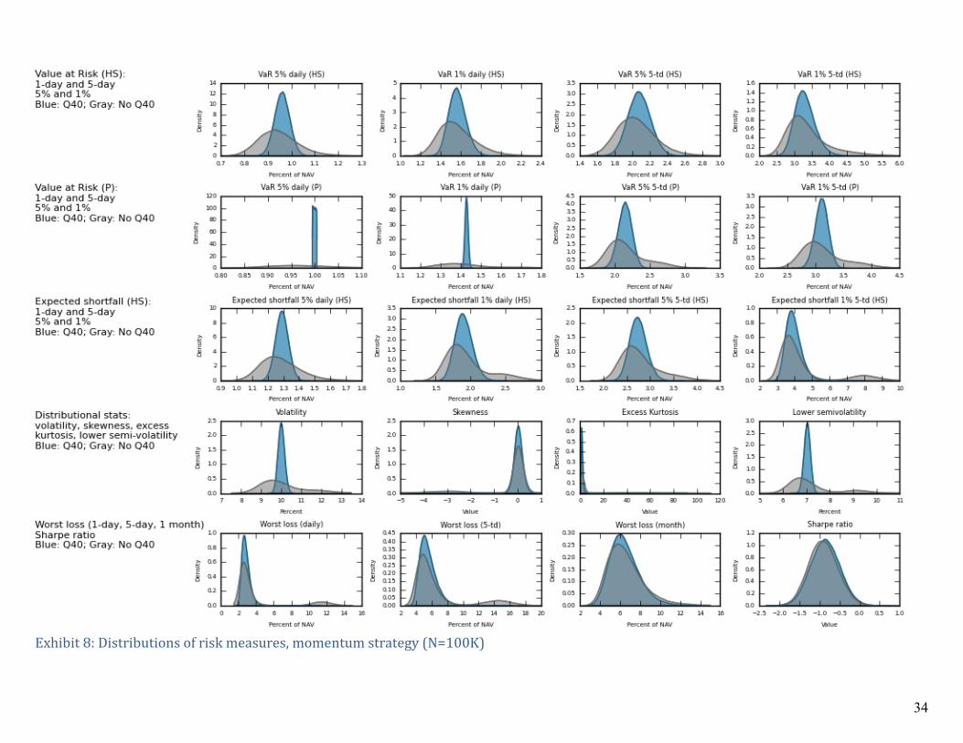
The results of the exercise appear in the histograms of portfolio risk measures in Exhibits 7 and 8. Exhibit 7 shows the results for the factor-alpha strategy, while Exhibit 8 shows the results for the momentum screen. Each histogram represents the measured risk for 100,000 randomly chosen portfolios that: (a) faithfully implement the chosen quantitative strategy; and (b) have the identical presentation to regulators on Form PF, as described in Exhibit 6, with the only exception being their treatment of Question 40: blue histograms represent portfolios constrained to have daily, 5 percent parametric VaR of 1.00 percent, while gray histograms represent portfolios without such a VaR constraint.24 Note that these distributions are not a statement regarding how investment advisers would or should manage their portfolios. Actual advisers do not simply manage portfolio risk, but must balance trade-offs among many factors, such as expected returns and alpha, fund marketing strategies, market liquidity, tax efficiency, etc. Rather, the histograms assess the error tolerances of Form PF as a risk-measurement instrument. They indicate the range within which actual portfolio risk levels can fluctuate without registering any change on the meter (i.e., on Form PF). The distributions thus indicate the accuracy with which regulators are able to measure the risks in hedge fund portfolios.

Summary statistics for risk measure distributions appear in Exhibits 9 and 10. Exhibit 9 provides summary statistics for the constrained VaR case (the blue histograms in Exhibits 7 and 8) while Exhibit 10 provides summary statistics in the unconstrained case (the gray

24 That is, funds with portfolios that do not have the VaR constraint have answered “No” to Question 40(a), which asks whether the fund regularly calculates VaR.

25

histograms in Exhibit 7 and 8). Aside from the summary statistics, we calculate three tolerance ratios in Exhibits 9 and 10 to help assess the risk measurement accuracy of Form PF. For a given distribution, the first tolerance ratio, TR1, is defined to be the ratio of the maximal value to the median value; the second tolerance ratio, TR2, is the ratio of the difference between the maximum and minimum values to the median value; and the third tolerance ratio, TR3, is defined to be the ratio of the interquartile range to the median value.

If the dispersion in a distribution is small, then we generally expect it to have a small standard deviation, and the three tolerance ratios defined above to have values close to one, zero, and zero, respectively. As is evident in Exhibit 9, however, dispersion in actual risk levels is significant and pervasive, even after constraining daily, 5 percent parametric VaR to be 1.00 percent. For both the factor-alpha and momentum screens, and for almost all VaR and expected shortfall risk statistics, the maximum actual risk is about 25 to 50 percent larger than the median actual risk, as indicated by the measure TR1. The 1-day, 5 percent, parametric VaR is constrained, of course, so this measure has an approximately uniform distribution over a very narrow range of values, all of which are equal when rounded to two decimal places of a percentage point. Unsurprisingly, the 1-day, 1 percent parametric VaR is closely correlated, and shows very little variability. On the other hand, 5-day VaRs and expected shortfall statistics show considerable range. The maximum 5-day, 1 percent historical VaR is about 75 percent larger than the median for the factor alpha strategy and is roughly 50 percent larger than the median for the momentum strategy; for 5-day, 1 percent expected shortfall, the maximum is nearly double the median. Comparing the maximum to the minimum observed values reveals a range that is approximately double the maximum-median range in most cases, since the risk measures are roughly symmetrically distributed. The measures of returns skewness and excess kurtosis are exceptions to these general results. The central limit theorem affects the sampling of expected returns across the 25,000 portfolios, forcing the cross-sectional distributions to be close to standard normal and restricting skewness and excess kurtosis.

We emphasize that these results represent lower bounds on the ranges of risk statistics available to more realistic portfolios. Our methodology utilizes plain-vanilla, purely quantitative, portfolio formation rules involving only listed U.S. equities. The intent is an isolated and unbiased assessment of Form PF as a risk-measurement instrument, rather than “fishing” for extreme strategies (such as the out-of-the-money puts in Lo’s [2001] Capital Decimation Partners parable) that a shrewd manager might abuse to overload a portfolio

26

with risk. Nonetheless, it would be straightforward to add listed equity options to the portfolios, and this remains a topic for future research. While it is clear that expanding the portfolio strategy space cannot reduce the maximum feasible risk, the magnitude of the possible increases in portfolio risk is an empirical question.

Finally, we examine the effectiveness of stratifying risk reports by VaR (Form PF Question 40) by considering the differences between the blue and gray histograms in Exhibits 7 and 8, as well as Exhibit 10. Removing this constraint opens the range of accessible risk levels significantly, doubling or tripling the maximum feasible exposure for most of our risk measures. This validates the use of VaR stratification on Form PF, and suggests that additional reporting of a more diverse set of risk measures could improve the precision of the form’s risk measurement. It also confirms the usefulness of the constrained-maximization technique as a methodology for testing the effectiveness of different reporting specifications.

This paper presents a novel methodology for assessing the risk-measurement tolerances of Form PF. Applying the method to plausible examples of quantitative hedge fund strategies over portfolios of listed equities reveals significant measurement tolerances in Form PF as a risk-measurement instrument. As a result, Form PF submissions may obscure reporting funds’ actual risks. A natural way to tighten these tolerances would be to re-stratify the characteristics that Form PF uses to represent complex portfolios, or to capture additional characteristics on the form to constrain the range of possible risk profiles more tightly. The methodology of constrained risk maximization provides a possible tool to help guide the choice of measurement dimensions for this purpose.

27

5. References

Adrian, T. (2007), “Measuring Risk in the Hedge Fund Sector,” Current Issues in Economics and Finance, Federal Reserve Bank of New York, 13(3), March/April.

Adrian, T.; Brunnermeier, M. K. & Nguyen, H.-L. Q. (2013), “Hedge Fund Tail Risk,” in

Joseph G. Haubrich & Andrew W. Lo, ed., Quantifying Systemic Risk, U. of Chicago Press, pp. 155–172.

Agarwal, V.; Daniel, N. D. & Naik, N. Y. (2011), “Do hedge funds manage their reported

returns?” Review of Financial Studies, 24, 3281–3320. Agarwal, V.; Gay, G. D. & Ling, L. (2014), “Window Dressing in Mutual Funds,” Review of

Financial Studies, forthcoming. http://ssrn.com/abstract=1804939 Amin, G. S. & Kat, H. M. (2003), “Welcome to the dark side: hedge fund attrition and

survivorship bias over the period 1994-2001,” J. of Alternative Investments 6(1), 57–73. Boyson, N. M., Stahel, C. W. and Stulz, R. M. (2010), “Hedge Fund Contagion and Liquidity

Shocks,” J. of Finance, 65(5), October, 1789-1816. Carhart, M. M. (1997), “On persistence in mutual fund performance,” J. of Finance, 52(1), 57–

82. Commodity Futures Trading Commission; Securities and Exchange Commission (CFTC-

SEC) (2011), “Reporting by Investment Advisers to Private Funds and Certain Commodity Pool Operators and Commodity Trading Advisers on Form PF: Final Rule,” Federal Register 76(221), 71128–71239.

Dixon, L.; Clancy, N. & Kumar, K. B. (2012), “Hedge Funds and Systemic Risk,” technical

report, RAND Corporation. http://www.rand.org/content/dam/rand/pubs/monographs/2012/RAND_MG1236.pdf

Dudley, E. and Nimalendran, M. (2011), “Margins and Hedge Fund Contagion,” J. of

Financial and Quantitative Analysis, 46(5), October, 1227-1257. Duffie, D. (2014), “Systemic Risk Exposures: A 10-by-10-by-10 Approach,” in Markus K.

Brunnermeier & Arvind Krishnamurthy, ed., Risk Topography: Systemic Risk and Macro Modeling, U. of Chicago Press, 47–56.

Elton, E. J.; Gruber, M. J.; Blake, C. R.; Krasny, Y. & Ozelge, S. O. (2010), “The effect of

holdings data frequency on conclusions about mutual fund behavior,” J. of Banking and Finance 34(5), 912–922.

28

Fama, E. F. & French, K. R. (1993), “Common risk factors in the returns on stocks and

bonds,” J. of Financial Economics 33(1), 3–56. ________ (1992), “The cross-section of expected stock returns,” J. of Finance 47(2), 427–465. Federal Financial Institutions Examination Council (FFIEC) (2014), “Consolidated Reports

of Condition and Income for a Bank with Domestic Offices Only – FFIEC 041,”reporting form, December. https://www.ffiec.gov/pdf/FFIEC_forms/FFIEC041_201412_f.pdf

Financial Crisis Inquiry Commission (FCIC) (2011), The Financial Crisis Inquiry Report: Final

Report of the National Commission on the Causes of the Financial and Economic Crisis in the United States, U.S. Government Printing Office.

Financial Stability Oversight Council (FSOC) (2014a) Annual Report 2014, FSOC.

http://www.treasury.gov/initiatives/fsoc/studies-reports/Pages/2014-Annual-Report.aspx

________(2014b), “Notice Seeking Comment on Asset Management Products and

Activities,” Federal Register, 79(247), December 24, 77488–77495. http://www.gpo.gov/fdsys/pkg/FR-2014-12-24/pdf/2014-30255.pdf

Foster, D. P. & Young, H. P. (2010), “Gaming performance fees by portfolio managers,”

Quarterly J. of Economics 125(4), 1435–1458. French, K. (2014), “Current Research Returns,” Internet site, Dartmouth U., 2014.

http://mba.tuck.dartmouth.edu/pages/faculty/ken.french/data_library.html Fung, W. & Hsieh, D. A. (2001), “The risk in hedge fund strategies: theory and evidence

from trend followers,” Review of Financial Studies, 14(2), April, 313–341. ________ (2004), “Hedge Fund Benchmarks: A Risk-Based Approach,” Financial Analysts J.,

60(5), September-October, 65–80. Getmansky, M.; Lo, A. W. & Makarov, I. (2004), “An econometric model of serial

correlation and illiquidity in hedge fund returns,” J. of Financial Economics 74(3), 529–609. Goetzmann, W. N.; Ingersoll, J. E. & Ross, S. A. (2003) “High-Water Marks and Hedge

Fund Management Contracts,” J. of Finance, 58, 1685–1718. Goetzmann, W.; Ingersoll, J.; Spiegel, M. & Welch, I. (2007), “Portfolio performance

manipulation and manipulation-proof performance measures,” Review of Financial Studies 20(5), 1503–1546.

29

Greene, N. J. (2013), “SEC JOBS Act Rulemaking Creates Opportunities and Potential

Burdens for Hedge Funds Contemplating General Solicitation and Advertising,” Hedge Fund Law Report, 6(28), July.

Griffiths, M. D. & Winters, D. B. (2005), “The Turn of the Year in Money Markets: Tests of

the Risk-Shifting Window Dressing and Preferred Habitat Hypotheses,” J. of Business 78(4), 1337–1364.

Gropp, R. (2014), “How Important Are Hedge Funds in a Crisis?” FRBSF Economic Letter

2014-11, April. Hodder, J. E. & Jackwerth, J. C. (2007), “Incentive Contracts and Hedge Fund

Management,” J. of Financial and Quantitative Analysis, 42, 811–826. House Committee on Financial Services (2007), Systemic Risk: Examining Regulators’ Ability to

Respond to Threats to the Financial System, Hearing before the Committee on Financial Services, U.S. House of Representatives, 110th Congress, October 2, 2007. http://www.gpo.gov/fdsys/pkg/CHRG-110hhrg39903/pdf/CHRG-110hhrg39903.pdf

Jacobs, B. & Levy, K. (1997), “The Long and Short on Long-Short,” J. of Investing, 6(1),

Spring, 73–88. Jegadeesh, N. (1990), “Evidence of predictable behavior of security returns,” J. of Finance,

45(3), 881–898. Jegadeesh, N. & Titman, S. (1993), “Returns to buying winners and selling losers:

Implications for stock market efficiency,” J. of Finance, 48(1), 65–91. ________ (2011), “Momentum,” Annual Review of Financial Economics, Annual Reviews, 3,

493-509. Joint Committee for Guides in Metrology, Working Group 1 (JCGM/WG1) (2008),

“Evaluation of measurement data -- Guide to the expression of uncertainty in measurement,” technical report JCGM 100:2008, 2008. http://www.bipm.org/utils/common/documents/jcgm/JCGM_100_2008_E.pdf

Khandani, A. & Lo, A. W. (2011), “What Happened To The Quants In August 2007?:

Evidence from Factors and Transactions Data,” J. of Financial Markets 14, 1–46. Lakonishok, J.; Shleifer, A.; Thaler, R. & Vishny, R. (1991), “Window Dressing by Pension

Fund Managers,” American Economic Review 81(2), 227–31. Lan, Y.; Wang, N. & Yang, J. (2013), “The economics of hedge funds,” J. of Financial

30

Economics, 110(2), 300–323. Li, D.; Markov, M. & Wermers, R. (2013) “Monitoring Daily Hedge Fund Performance,” J.

of Investment Consulting, 14(1), 57–68. Lo, A. W. (2008), “Hedge Funds, Systemic Risk, and the Financial Crisis of 2007-2008:

Written Testimony for the House Oversight Committee Hearing on Hedge Funds,” MIT, November 13, 2008. http://ssrn.com/abstract=1301217

________ (2001), “Risk management for hedge funds: Introduction and overview,” Financial

Analysts J., 16–33. Lo, A. W. and Patel, P. N. (2008), “130/30: The New Long-Only,” J. of Portfolio Management,

34(2), 12–38. López de Prado, M. & Peijan, A. (2004), “Measuring Loss Potential of Hedge Fund

Strategies,” J. of Alternative Investments, 7(1), Summer, 7–31. Mitchell, M. and Pulvino, T. (2012), “Arbitrage crashes and the speed of capital,” J. of

Financial Economics, 104(3), June, 469–490. Munyan, B. (2014), “Regulatory Arbitrage in Repo Markets,” working paper, U. of Maryland.

http://www.bmunyan.com/ Office of Financial Research (OFR) (2014), Annual Report 2014, technical report, December.

http://www.treasury.gov/initiatives/ofr/about/Documents/OFR_AnnualReport2014_FINAL_12-1-2014.pdf

Ortiz, C.; Sarto, J. L. & Vicente, L. (2012), “Portfolios in disguise? Window dressing in bond

fund holdings “, J. of Banking and Finance, 36(2), 418–427. Parry, H. (2001), “Hedge Funds, Hot Markets and the High Net Worth Investor: A Case for

Greater Protection,” Northwestern J. of International Law and Business 21(3), 703–722. Patton, A. J. & Ramadorai, T. (2013), “On the High-Frequency Dynamics of Hedge Fund

Risk Exposures,” J. of Finance, 68(2), 597–635. Price Waterhouse Coopers (PWC) (2011), “Reporting by Private Fund Advisers on Form

PF: SEC and CFTC Adopt Final Rules Requiring Registered Advisers to Private Funds to File New Form PF,' Technical report, November. http://www.pwc.com/us/en/financial-services/regulatory-services/publications/assets/closer-look-final-rule-private-fund-advisers-form-pf.pdf

Securities and Exchange Commission (SEC) (2015), “Form PF: Frequently Asked

31

Questions,” technical document, accessed 16 March 2015. http://www.sec.gov/divisions/investment/pfrd/pfrdfaq.shtml.

________ (2014a), “Annual Staff Report Relating to the Use of Data Collected from Private

Fund Systemic Risk Reports,” technical report, August. http://www.sec.gov/reportspubs/special-studies/im-private-fund-annual-report-081514.pdf

________ (2014b), “List of Section 13F Securities: Fourth Quarter FY 2014,” technical

document, December. http://www.sec.gov/divisions/investment/13f/13flist2014q4.pdf

________ (2013), “Hedge Funds,” Investor Bulletin, February. http://investor.gov/news-

alerts/hedge-funds ________ (2011a), “FORM PF: Reporting Form for Investment Advisers to Private Funds

and Certain Commodity Pool Operators and Commodity Trading Advisers,” reporting form SEC 2048 (OMB Number: 3235-0679). http://www.sec.gov/about/forms/formpf.pdf

________ (2011b), “Form ADV: General Instructions,” technical document.

http://www.sec.gov/about/forms/formadv-instructions.pdf ________ (1997), “Privately Offered Investment Companies,” Federal Register, 62(68),

17512–17529. http://www.gpo.gov/fdsys/pkg/FR-1997-04-09/pdf/97-8950.pdf ________ (1992), “Protecting Investors: A Half Century of Investment Company

Regulation,” SEC Division of Investment Management. http://www.sec.gov/divisions/investment/guidance/icreg50-92.pdf

Sialm, C., Sun, Z. and Zheng, L. (2013), “Home Bias and Local Contagion: Evidence from

Funds of Hedge Funds,” NBER Working Paper w19570. http://www.nber.org/papers/w19570.

Sias, R. (2007), “Causes and Seasonality of Momentum Profits,” Financial Analysts J., 63(2),

48–54. Sias, R. W. & Starks, L. T. (1997), “Institutions and Individuals at the Turn-of-the-Year,” J.

of Finance, 52(4), 1543–1562. U.S. Congress (1996), “National Securities Markets Improvement Act of 1996,” October.

http://www.gpo.gov/fdsys/pkg/PLAW-104publ290/pdf/PLAW-104publ290.pdf. ________ (2010), “Dodd-Frank Wall Street Reform and Consumer Protection Act,” July.

32

http://www.gpo.gov/fdsys/pkg/PLAW-111publ203/pdf/PLAW-111publ203.pdf Wermers, R. (2012), “Matter of Style: The Causes and Consequences of Style Drift in

Institutional Portfolios,” working paper, U. of Maryland. http://ssrn.com/abstract=2024259

White, M. J. (2014), “Enhancing Risk Monitoring and Regulatory Safeguards for the Asset

Management Industry,” Speech to The New York Times DealBook Opportunities for Tomorrow Conference, New York City, Dec. 11, 2014, Securities and Exchange Commission. http://www.sec.gov/News/Speech/Detail/Speech/1370543677722#.VMLSvfldVCY

33

Exhibit 7: Distributions of risk measures, factor-alpha strategy (N=100K)

34

Exhibit 8: Distributions of risk measures, momentum strategy (N=100K)

35

Exhibit 9: Risk measurement tolerances in Form PF with VaR constraint (N=100K) Source: CRSP, OFR analysis

Factor alpha strategy Momentum strategy

Risk measure Avg StD Min 25% 50% 75% Max TR1 TR2 TR3 Avg StD Min 25% 50% 75% Max TR1 TR2 TR3 Value at Risk, hist. sim. 5% over 1 trading day 0.93 0.04 0.74 0.91 0.93 0.96 1.08 1.16 0.36 0.05 0.96 0.03 0.76 0.94 0.96 0.98 1.11 1.16 0.37 0.05

Value at Risk, hist. sim. 1% over 1 trading day 1.56 0.09 1.21 1.50 1.56 1.62 2.11 1.36 0.58 0.08 1.57 0.09 1.27 1.51 1.56 1.62 2.04 1.30 0.49 0.07

Value at Risk, hist. sim. 5% over 5 trading days 1.74 0.12 1.29 1.66 1.74 1.82 2.32 1.33 0.59 0.09 2.08 0.13 1.45 1.99 2.07 2.16 2.63 1.27 0.57 0.08

Value at Risk, hist. sim. 1% over 5 trading days 2.98 0.28 2.01 2.79 2.96 3.15 4.94 1.67 0.99 0.12 3.30 0.29 2.32 3.09 3.27 3.47 5.03 1.54 0.83 0.12

Value at Risk, parametric 5% over 1 trading day 1.00 0.00 1.00 1.00 1.00 1.00 1.00 1.00 0.01 0.01 1.00 0.00 1.00 1.00 1.00 1.00 1.00 1.01 0.01 0.01

Value at Risk, parametric 1% over 1 trading day 1.46 0.01 1.45 1.46 1.46 1.47 1.49 1.02 0.03 0.01 1.43 0.01 1.40 1.42 1.43 1.44 1.46 1.02 0.04 0.01

Value at Risk, parametric 5% over 5 trading days 1.88 0.09 1.50 1.82 1.87 1.93 2.26 1.20 0.40 0.06 2.14 0.10 1.68 2.08 2.14 2.21 2.53 1.18 0.40 0.06

Value at Risk, parametric 1% over 5 trading days 2.90 0.12 2.37 2.82 2.90 2.98 3.44 1.19 0.37 0.06 3.11 0.12 2.57 3.03 3.11 3.19 3.60 1.16 0.33 0.05

Expected shortfall 5% over 1 trading day 1.27 0.04 1.04 1.24 1.27 1.30 1.47 1.15 0.34 0.05 1.29 0.04 1.10 1.26 1.29 1.32 1.47 1.14 0.29 0.04

Expected shortfall 1% over 1 trading day 1.90 0.12 1.43 1.82 1.89 1.98 2.57 1.36 0.60 0.08 1.90 0.12 1.49 1.82 1.90 1.98 2.49 1.32 0.53 0.09

Expected shortfall 5% over 5 trading days 2.42 0.17 1.78 2.30 2.41 2.53 3.20 1.33 0.59 0.09 2.74 0.18 2.03 2.62 2.74 2.86 3.73 1.36 0.62 0.09

Expected shortfall 1% over 5 trading days 3.67 0.46 2.36 3.34 3.61 3.94 6.69 1.85 1.20 0.16 3.95 0.44 2.63 3.64 3.90 4.21 8.04 2.06 1.39 0.15

Volatility Annualized 10.8 0.09 10.4 10.7 10.8 10.8 11.2 1.04 0.07 0.01 10.0 0.16 9.37 9.90 10.0 10.1 10.6 1.06 0.13 0.02

Skewness 1 trading day 0.29 0.24 -0.70 0.14 0.25 0.40 4.05 16.0 18.7 1.02 0.05 0.20 -5.29 -0.07 0.05 0.16 2.00 43.4 158 5.04

Excess kurtosis 1 trading day 2.60 2.11 0.17 1.52 2.06 2.89 58.9 28.6 28.5 0.66 1.92 1.35 0.21 1.35 1.74 2.26 91.7 52.6 52.4 0.52

Lower semivol Annualized 7.43 0.14 6.39 7.34 7.44 7.52 7.95 1.07 0.21 0.02 7.04 0.14 6.35 6.95 7.05 7.14 8.04 1.14 0.24 0.03

Worst loss 1 trading day 2.81 0.43 1.75 2.51 2.75 3.05 6.99 2.54 1.91 0.20 2.84 0.49 1.74 2.51 2.77 3.09 11.4 4.12 3.49 0.21

Worst loss 5 trading days 5.25 1.03 2.83 4.49 5.10 5.84 13.6 2.68 2.13 0.26 5.53 1.05 3.08 4.78 5.36 6.11 16.4 3.06 2.49 0.25

Worst loss Monthly 3.81 1.17 0.66 2.98 3.68 4.50 11.0 3.01 2.83 0.41 6.47 1.46 2.39 5.44 6.30 7.32 15.5 2.46 2.09 0.30

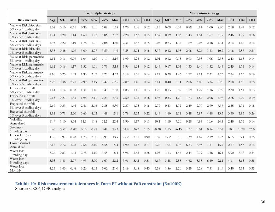
36

Exhibit 10: Risk measurement tolerances in Form PF without VaR constraint (N=100K) Source: CRSP, OFR analysis

Factor alpha strategy Momentum strategy

Risk measure Avg StD Min 25% 50% 75% Max TR1 TR2 TR3 Avg StD Min 25% 50% 75% Max TR1 TR2 TR3 Value at Risk, hist. sim. 5% over 1 trading day 1.02 0.10 0.71 0.96 1.01 1.08 1.78 1.76 1.06 0.12 0.95 0.09 0.67 0.89 0.94 1.00 2.05 2.18 1.47 0.12

Value at Risk, hist. sim. 1% over 1 trading day 1.74 0.20 1.14 1.60 1.72 1.86 3.92 2.28 1.62 0.15 1.57 0.19 1.03 1.43 1.54 1.67 3.79 2.46 1.79 0.16

Value at Risk, hist. sim. 5% over 5 trading days 1.93 0.22 1.19 1.78 1.91 2.06 4.40 2.31 1.68 0.15 2.05 0.23 1.37 1.89 2.03 2.18 4.34 2.14 1.47 0.14

Value at Risk, hist. sim. 1% over 5 trading days 3.33 0.48 1.99 3.00 3.27 3.59 11.6 3.55 2.94 0.18 3.37 0.62 1.95 2.96 3.24 3.63 10.2 3.16 2.56 0.21

Value at Risk, parametric 5% over 1 trading day 1.11 0.11 0.79 1.04 1.10 1.17 2.19 1.99 1.26 0.12 1.01 0.12 0.73 0.93 0.98 1.06 2.38 2.43 1.68 0.14

Value at Risk, parametric 1% over 1 trading day 1.62 0.16 1.17 1.52 1.61 1.71 3.15 1.96 1.24 0.12 1.44 0.17 1.04 1.33 1.40 1.52 3.44 2.45 1.71 0.14

Value at Risk, parametric 5% over 5 trading days 2.10 0.25 1.39 1.93 2.07 2.23 4.52 2.18 1.51 0.14 2.17 0.29 1.43 1.97 2.11 2.31 4.73 2.24 1.56 0.16

Value at Risk, parametric 1% over 5 trading days 3.22 0.36 2.21 2.99 3.19 3.42 6.65 2.09 1.40 0.14 3.14 0.40 2.14 2.86 3.06 3.34 6.98 2.28 1.58 0.15

Expected shortfall 5% over 1 trading day 1.41 0.14 0.98 1.31 1.40 1.49 2.58 1.85 1.15 0.13 1.28 0.13 0.87 1.19 1.27 1.36 2.92 2.30 1.61 0.13

Expected shortfall 1% over 1 trading day 2.13 0.27 1.35 1.95 2.11 2.29 5.46 2.60 1.95 0.16 1.95 0.33 1.20 1.73 1.87 2.08 4.98 2.66 2.02 0.19

Expected shortfall 5% over 5 trading days 2.69 0.33 1.66 2.46 2.66 2.88 6.30 2.37 1.75 0.16 2.79 0.43 1.72 2.49 2.70 2.99 6.36 2.35 1.71 0.18

Expected shortfall 1% over 5 trading days 4.12 0.71 2.20 3.63 4.02 4.49 15.1 3.78 3.23 0.22 4.44 1.60 2.14 3.48 3.87 4.48 13.5 3.50 2.95 0.26

Volatility Annualized 11.9 1.10 8.64 11.1 11.8 12.5 22.4 1.90 1.17 0.11 10.1 1.19 7.20 9.28 9.84 10.6 24.4 2.49 1.76 0.14

Skewness 1 trading day 0.40 0.52 -1.42 0.15 0.29 0.49 9.23 31.8 36.7 1.15 -0.38 1.15 -6.45 -0.15 0.01 0.14 5.57 500 1079 26.0

Excess kurtosis 1 trading day 4.35 7.97 0.28 1.75 2.50 3.99 193 77.2 77.1 0.90 8.59 17.2 0.16 1.39 1.87 2.79 122 65.5 65.4 0.75

Lower semivol Annualized 8.16 0.72 5.98 7.66 8.10 8.58 15.4 1.90 1.17 0.11 7.22 1.04 4.96 6.53 6.93 7.51 15.7 2.27 1.55 0.14

Worst loss 1 trading day 3.26 0.83 1.63 2.75 3.10 3.55 18.4 5.96 5.43 0.26 4.03 3.13 1.47 2.44 2.79 3.38 16.4 5.90 5.38 0.34

Worst loss 5 trading days 5.93 1.41 2.77 4.93 5.70 6.67 22.2 3.91 3.42 0.31 6.67 3.48 2.58 4.62 5.38 6.69 22.1 4.11 3.63 0.38

Worst loss Monthly 4.25 1.43 0.46 3.26 4.05 5.02 21.0 5.19 5.08 0.43 6.58 1.86 2.20 5.29 6.28 7.51 21.9 3.49 3.14 0.35