Gaseous Species Measurements of Alternative Jet Fuels in

Sooting Laminar Coflow Diffusion Flames

by

Parham Zabeti

A thesis submitted in conformity with the requirements

for the degree of Master of Applied Science

Graduate Department of Mechanical and Industrial Engineering

University of Toronto

© Copyright by Parham Zabeti 2010

ii

Abstract

Gaseous Species Measurements of Bio-Jet Fuels in a Laminar Coflow Diffusion Flame

Parham Zabeti

Master of Applied Science

Graduate Department of Mechanical and Industrial Engineering

University of Toronto

2010

The gaseous species concentration of Jet A-1, GTL, CTL and a blend of 80 vol.% GTL and 20

vol.% hexanol jet fuels in laminar coflow diffusion flames have been measured and studied. These

species are carbon monoxide, carbon dioxide, oxygen, methane, ethane, ethylene, propylene, and

acetylene. Benzene and propyne concentrations were also detected in CTL flames. 1-Butene has

been quantified for the blend of GTL and hexanol flame.

The detailed experimental setup has been described and results from different flames are

compared. The CO is produced in a same amount in all the flames. The CTL flame had the

largest and GTL/hexanol flame had lowest CO2 concentrations. The results indicate that GTL

and GTL hexanol blend flames produce similar concentrations for all the measured hydrocarbon

species and have the highest concentration among all the jet fuels. The experimental results from

Jet A-1 fuel are also compared with numerical studies by Saffaripour et al.

iii

Dedication

To Tiam, my adorable new born nephew, and to all future generations.

May the world be a peaceful place for them to grow, fall in love and flourish.

iv

Acknowledgments

I would like to thank my mother whose patience and blessing made choosing the right path for

my life possible. My greatest appreciation to my always supportive brother, Pedram. Without his

encouragement and insight, I would never reach where I am today.

My extended gratitude goes to Professor Murray Thomson for his comprehensive prospect

and wise judgement on this project. Murray has been an inspiration to my academic and personal

lives throughout my studies at the University of Toronto.

I am grateful to know Mahsa, my best friend during last two years. With no doubt she will

be one of the most sincere, intelligent and friendliest characters I would ever encounter in my

life. My thesis also benefits from her artistic talents in some of the drawings in this dissertation.

Thank you for being there for me in all the ups and downs.

Gratefulness to my colleagues at Combustion Research Group, specifically my labmates,

Meghdad Saffaripour, Coleman Yeung and Carlos Martinez who created a warm and welcoming

work environment. A special thanks to my former colleague, Dr. Mani Sarathy who helped me

since the first days of my graduate studies from answering my endless questions to setting up my

experimental apparatus. His step by step teaching throughout my first year of Master’s is much

appreciated. I still always enjoy our conversations and try to learn from you. Also, I was fortunate

to learn a lot from other talented group members such as Dr. Seth Dworkin.

v

I would also like to acknowledge OGS, ALFA-BIRD for funding this study and NRC for

donating the burner to the Combustion Research Group.

vi

List of Content

ABSTRACT ........................................................................................................................................................ II

DEDICATION ................................................................................................................................................. III

ACKNOWLEDGMENTS ................................................................................................................................ IV

LIST OF CONTENT ........................................................................................................................................ VI

LIST OF TABLES ............................................................................................................................................. IX

LIST OF FIGURES ............................................................................................................................................ X

LIST OF APPENDICES ................................................................................................................................ XIV

ACRONYMS ................................................................................................................................................... XV

1. INTRODUCTION ..................................................................................................................................... 1

1.1 RESEARCH MOTIVATION .............................................................................................................................. 2

1.2 RESEARCH OBJECTIVES ................................................................................................................................. 3

1.3 RESEARCH EXECUTION ................................................................................................................................. 4

2. BACKGROUND RESEARCH .................................................................................................................. 5

2.1 AVIATION FUELS ............................................................................................................................................ 5

2.1.1 Physical and Chemical Properties .............................................................................................................. 6

2.1.2 Proposed Alternative Jet Fuels .................................................................................................................. 9

2.1.2.1 Fischer-Tropsch Synthetic Kerosene ........................................................................................................... 9

2.1.2.2 Bio-Derived Synthetic Paraffinic Kerosene (or BTL) ............................................................................... 13

vii

2.1.2.3 Bio-Alcohols .............................................................................................................................................. 14

2.1.2.4 Other Blends .............................................................................................................................................. 15

2.1.3 Surrogate of Jet Fuels ............................................................................................................................. 15

2.2 JET ENGINE DESIGN .................................................................................................................................... 16

2.2.1 Emissions .............................................................................................................................................. 17

2.3 FUNDAMENTALS OF COFLOW LAMINAR DIFFUSION FLAME ................................................................... 18

2.3.1 Governing Equations for Laminar Diffusion Flame ............................................................................... 20

2.3.2 Flame Liftoff ......................................................................................................................................... 20

2.3.3 Flame Length (or Visible Flame Height) ................................................................................................ 20

2.4 SOOT FORMATION IN COFLOW FLAMES ................................................................................................... 22

3. EXPERIMENTAL APPARATUS & ANALYTICAL METHODOLOGY .......................................... 28

3.1 FUEL SUPPLY ................................................................................................................................................ 30

3.2 FUEL VAPORIZATION SYSTEM .................................................................................................................... 33

3.3 COFLOW DIFFUSION FLAME BURNER ........................................................................................................ 36

3.3.1 What is a Suitable Flame? ..................................................................................................................... 37

3.4 EXPERIMENTAL TEMPERATURE AND FLOW SETTINGS ............................................................................ 39

3.4.1 Flow Controls ....................................................................................................................................... 39

3.4.2 Temperature Settings ............................................................................................................................. 40

3.5 GAS SAMPLING SYSTEM .............................................................................................................................. 41

3.5.1 Sampling Apparatus .............................................................................................................................. 41

3.5.2 Sampling Procedure ............................................................................................................................... 44

3.5.2.1 Detecting the Leaks ................................................................................................................................... 44

3.5.2.2 Centring the Burner ................................................................................................................................... 46

3.5.2.3 Sampling the Flame ................................................................................................................................... 47

viii

3.6 ANALYTICAL TECHNIQUES ......................................................................................................................... 50

3.6.1 Principles of Gas Chromatography .......................................................................................................... 50

3.6.1.1 GC–TCD .................................................................................................................................................. 51

3.6.1.2 GC–FID .................................................................................................................................................... 53

3.6.1.3 Calibration of Gas Chromatography ......................................................................................................... 56

3.6.2 Non-Dispersive Infrared Analysis .......................................................................................................... 59

4. RESULTS & DISCUSSIONS .................................................................................................................. 61

4.1 JET A-1 FLAME............................................................................................................................................. 62

4.2 GAS-TO-LIQUID FLAME .............................................................................................................................. 70

4.3 COAL-TO-LIQUID FLAME ........................................................................................................................... 73

4.4 GAS-TO-LIQUID BLEND WITH HEXANOL FLAME .................................................................................... 76

4.5 SPECIES COMPARISON ................................................................................................................................. 78

4.6 COMPARISON WITH COFLOW ETHYLENE DIFFUSION FLAME ................................................................. 84

5. CONCLUSIONS & RECOMMENDATIONS ...................................................................................... 86

5.1 CONCLUSIONS .............................................................................................................................................. 86

5.2 IN-PROGRESS WORK ................................................................................................................................... 88

5.3 FUTURE WORKS ........................................................................................................................................... 88

5.3.1 Recommendations .................................................................................................................................. 89

BIBLIOGRAPHY .............................................................................................................................................. 91

APPENDICES ................................................................................................................................................. 100

ix

List of Tables

Table 2-1: Specific properties of aviation fuels including the experimented Jet A-1 ..................... 7

Table 2-2: Comparison between key thermochemical and physical properties of Shell Jet A-1,

ethanol and hexanol ...................................................................................................................... 14

Table 2-3: Surrogates for alternative jet fuels suggested by Dagaut et al .................................... 16

Table 2-4: Smoke point analysis of experimented jet fuel ........................................................... 27

Table 3-1: Summary of Jet A-1 composition analysis by group and carbon number ................. 31

Table 3-2: Specific heat capacity and thermal conductivity of experimental fuels ...................... 32

Table 3-3: Fuel flowrate settings on liquid flow controller in terms of C14H30 fuel flowrates ..... 39

Table 3-4: A sample of comparison between measured and literature FID relative molar response

factors for a range of organic molecules ....................................................................................... 59

Table 4-1: Acetylene level comparison in ethylene and Hex20-GTL coflow diffusion flames ... 84

x

List of Figures

Figure 2.1: Simplified block diagram of GTL process to produce FT-SPK .............................. 11

Figure 2.2: Simplified block diagram of Sasol CTL process to produce FSJF ........................... 12

Figure 2.3: Simplified block diagram of thermochemical conversion route for Bio-SPK ......... 13

Figure 2.4: A typical jet engine drawing showing the three main steps: compression, combustion,

expansion ...................................................................................................................................... 17

Figure 2.5: Soot formation and destruction zones in laminar diffusion flames ........................... 23

Figure 2.6: The H-abstraction–C2H2-addition (HACA) mechanism of PAH formation . ........ 24

Figure 2.7: A rough picture of soot formation ............................................................................ 25

Figure 3.1: Schematic diagram of the experimental setup ........................................................... 29

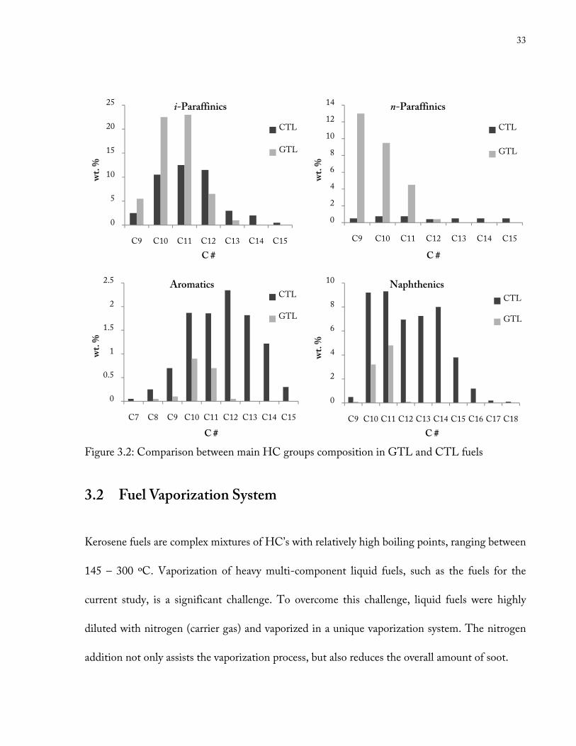
Figure 3.2: Comparison between main HC groups composition in GTL and CTL fuels .......... 33

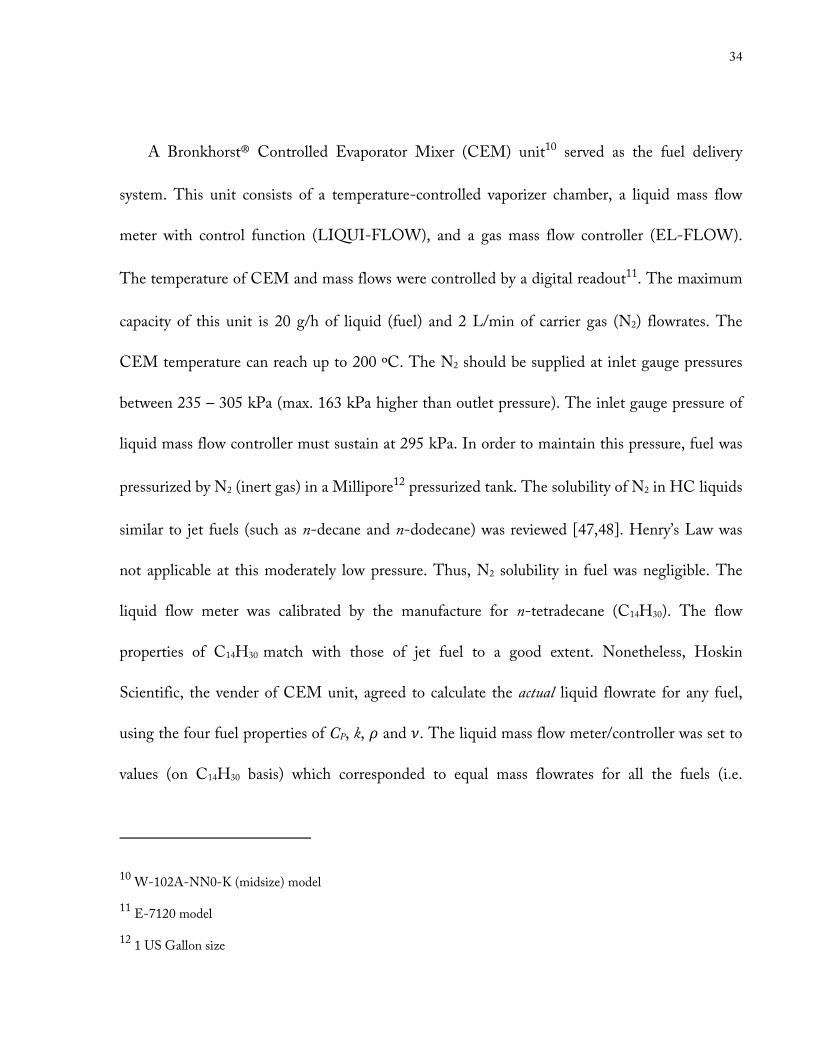
Figure 3.3: Bronkhorst® liquid delivery system with vapour control ........................................... 35

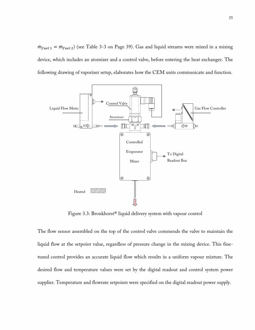
Figure 3.4: Schematic diagram and section cut of a coflow burner ............................................. 36

Figure 3.5: Schematic of microprobe head ................................................................................... 43

xi

Figure 3.6: The centring process ................................................................................................. 46

Figure 3.7: Schematic of dual column GC-TCD setup .............................................................. 52

Figure 3.8: Schematic of dual column GC-FID setup ................................................................ 54

Figure 3.9: GC-FID column oven temperature program ............................................................ 55

Figure 3.10: Permeation tube setup .............................................................................................. 57

Figure 4.1: Bottom portion of a typical Jet A-1 flame ................................................................ 62

Figure 4.2: Jet A-1 CO & CO2 centreline concentration profiles .............................................. 63

Figure 4.3: Jet A-1 CO & CO2 radial concentration profiles (a) z = 12 mm (b) z = 14 mm ..... 64

Figure 4.4: Jet A-1 centreline concentration profiles (a) CH4 & C2H6 (b) C2H4, C2H2 & C3H6 64

Figure 4.5: Jet A-1 species radial concentration profiles (a) z =12 mm, (b) z = 14 mm ............. 65

Figure 4.6: Computational (model) and experimental (exp) comparisons of CO & CO2 mole

fractions for Jet A-1 flame along (a) centreline and (b) radial (z = 12 mm) profiles ................... 66

Figure 4.7: Computational (model) and experimental (exp) comparison of species centreline

mole fractions for Jet A-1 flame along (a) CH4 & C2H6 (b) C2H4 & C2H2 (c) & C3H6 ........... 66

xii

Figure 4.8: Computed temperature isotherm for Jet A-1 laminar coflow diffusion flame by

Saffaripour et al. ........................................................................................................................... 67

Figure 4.9: GTL flame during sampling at the height of z = 30 mm in the flame ..................... 70

Figure 4.10: GTL jet fuel CO and CO2 centreline concentration profiles ................................. 71

Figure 4.11: GTL jet fuel species radial concentration profiles (a) z =14 mm, (b) z = 18 mm ... 71

Figure 4.12: GTL centreline concentration profiles (a) CH4 & C2H6 (b) C2H4, C2H2 & C3H6 . 72

Figure 4.13: CTL highly sooting flame ....................................................................................... 73

Figure 4.14: CTL jet fuel CO and CO2 centreline concentration profiles ................................. 74

Figure 4.15: CTL jet fuel centreline concentration profiles (a) CH4 & C2H6 (b) C2H4, C2H2 &

C3H6 (c) C3H4 & C6H6 ................................................................................................................ 75

Figure 4.16: Hex20-GTL jet fuel CO and CO2 centreline concentration profiles .................... 77

Figure 4.17: Hex20-GTL jet fuel centreline concentration profile (a) CH4 & C2H6 (b) C2H4,

C2H2 & C3H6 (c) C4H8 ................................................................................................................ 78

Figure 4.18: CO & CO2 centreline concentration profiles comparison of experimental fuels .. 79

Figure 4.19: Species centreline concentration comparison between CTL jet fuel and Jet A-1 ... 80

xiii

Figure 4.20: Species centreline concentrations comparison between CTL & GTL jet fuels ..... 81

Figure 4.21: Species centreline concentrations comparison between Jet A-1 & GTL jet fuels .. 82

Figure 4.22: Species centreline concentrations comparison between GTL & Hex20-GTL jet

fuels ............................................................................................................................................... 83

xiv

List of Appendices

Appendix A:

Part (I) – Jet A-1 Fuel Composition

Part (II) – Jet Fuels Thermophysical Properties

Part (III) – Jet A-1 Thermodynamic Properties

Appendix B:

Step by Step Sample Analysis of GC-TCD

Appendix C:

Sample Gas Chromatograms

Appendix D:

Governing Equations

Appendix E:

Sample Hand Calculation

xv

Acronyms

ALFA-BIRD Alternative Fuels and Biofuels for Aircraft Development

ARC Alberta Research Council

ASTM American Society for Testing and Materials

BTL Biomass-to-Liquid

CEM Controlled Evaporative Mixer

Ci Hydrocarbon with i number of carbon(s)

CTL Coal-to-Liquid

EFC Electronic Flow Control

FID Flame Ionization Detector

FS Fused Silica

FSJF Fully Synthetic Jet Fuel

FT Fischer-Tropsch

GC Gas Chromatography

GHG Green House Gas

GSV Gas Sampling Valve

GTL Gas-to-Liquid

xvi

HC Hydrocarbon

Hex20-GTL 20 vol.% Hexanol and 80 vol.% Gas-to-Liquid Blend

IATA International Air Transport Association

IFP Institut Francais du Petrole

LOD Limit of Detection

LOQ Limit of quantification

LPG Liquefied Petroleum Gas

NDIR Non-Dispersive Infrared

NG Natural Gas

NRC-IAR National Research Council Canada-Institute for Aerospace Research

PAH Polycyclic Aromatic Hydrocarbon

PM Particulate Matter

RT Retention Time

SPK Synthetic Paraffinic Kerosene

SS Stainless Steel

STP Standard Temperature Pressure

TCD Thermal Conductivity Detector

VOC Volatile Organic Compound

1

Chapter 1

1. Introduction

There is an emerging demand for alternative and sustainable energy sources to replace the

conventional non-renewable energy supply. Currently, aviation consumes about 8% of total fossil

fuels burned. This amount is equivalent to 12% of the fuel consumption of the entire

transportation sector, compared to 75 – 80% dedicated to road transport [1]. Particulate matter

(PM), volatile organic compounds (VOC’s), and greenhouse gases (GHG), such as carbon

dioxide (CO2), nitrogen oxides (NOX) and unburned hydrocarbons (HC) (e.g. methane)

emissions are in direct proportion to the fuel consumption.

Nonetheless, air traffic is steadily increasing (a 60% increase by 2020 is expected [2]), and

energy supply from conventional mineral kerosene fuel is decreasing. Unlike other transportation

sectors, aviation currently has no viable alternative to burning fossil fuels. Nuclear and electric

power are not suitable alternatives with current technologies [3]. Besides these concerns, volatile

fuel prices are damaging the airline industry. For example, Air Canada, and most recently, Japan

Airlines Corp. filed for bankruptcy mainly as a result of unstable fuel costs1.

1 Various sources and articles from Reuter’s News website (ca.reuters.com). Accessed on May 2010.

2

1.1 Research Motivation

The reduction of GHG emissions is the top priority in tackling global warming. A major source

of emissions, the transportation sector, including aviation, is working hard towards this goal.

Based on the reasons mentioned on the last page, scientists, politicians and economists are

investigating alternative fuels for aviation. The combustion study of alternative fuels is a vital part

of this investigation. Recently, European programs, such as Sustainable Way for Alternative

Fuels and Energy for Aviation and ALFA-BIRD (Alternative Fuels and Biofuels for Aircraft

Development), and American programs by Defense Energy Support Center and Air Force

Certification Office have begun to study and certify novel renewable fuels [4].

Organizations and research institutes, for instance the Sustainable Aviation Fuel User

Group and the Institut Francais du Petrole (IFP), are among the pioneer supporters of

alternative jet fuels. The latest goal of International Air Transport Association (IATA) is for its

members to be using a 6% mix of sustainable 2nd generation biofuels by 2020 [5]. On the other

hand, there is an immediate need for investigating the products of combustion of these

alternative aviation fuels. The current research project, as a segment of a larger study conducted

at the Combustion Research Laboratory2, is aimed to fulfill this goal.

2 Department of Mechanical and Industrial Engineering, at the University of Toronto

3

Numerous computational and experimental studies of kerosene-based fuel combustion have

been conducted in jet stirred reactors, shock tubes and flow tubes [6,7]. There are also a few

studies of jet fuel surrogate in non-sooting counterflow flames, such as work done by Humer and

Cooke et al. [8,9]. However, experimental studies of sooting jet fuel flames, i.e. Jet A-1, JP-8 or

any blend of different jet fuels in a laminar coflow flame, are very limited if any exists. Most

coflow flame studies were either done on simple gaseous fuels (such as ethylene (C2H4), methane

(CH4) or non-sooting surrogates) or there was only a trace of jet fuel in the fuel stream [10].

Experimental data, also, can be used to validate models of combustion chemistry and soot

formation. Findings from Jet A-1 and other alternative jet fuels in coflow combustion will lead to

better understanding of species concentration profiles in the flame, thermo-chemical mechanism

of combustion reactions, polycyclic aromatic hydrocarbon (PAH) formation and soot studies.

1.2 Research Objectives

The goal of this research project is to measure gaseous species in different jet fuel coflow

diffusion flames along the centreline, and where possible, several radii. The fuels used in the

current study are divided into two groups of conventional and Fischer-Tropsch (FT) kerosene jet

fuels. For this study, Jet A-1 has been used as a base fuel (i.e. conventional kerosene-based jet

fuel as a reference jet fuel). The experimental FT kerosene fuels include: (1) Gas-to-Liquid

(GTL), (2) Coal-to-Liquid (CTL), and (3) a blend of 80 vol.% GTL and 20 vol.% hexanol jet

fuels (Hex20-GTL). The final goal may be divided into the following specific three objectives:

4

• to develop a robust technique to obtain a stable flame for these complex liquid fuels;

• to sample gases in the most accurate manner to avoid any sample loss and minimize the

flame disturbance;

• to measure and interpret the concentration of major species in the flames.

1.3 Research Execution

The Jet A-1 was obtained from National Research Council Canada-Institute for Aerospace

Research (NRC-IAR), Gas Turbine Laboratory. The alternative fuels were provided through the

ALFA-BIRD international collaborative program between University of Toronto and research

institutes and companies in European Union and South Africa.

Flame studies were carried out at atmospheric pressure in a coflow diffusion flame. Gas

samples from the flame were analyzed using a number of experimental techniques. Hydrocarbon

concentrations were obtained by gas chromatography (GC) equipped with flame ionization

detectors (GC-FID). The carbon monoxide (CO) and CO2 concentrations were measured using

thermal conductivity detector gas chromatography (GC-TCD). A non-dispersive infrared

(NDIR) spectroscope was used to measure CO and CO2 concentrations in real-time. Details of

experimental apparatus and analytical methodology are described in Chapter 3. The experimental

species concentrations for Jet A-1 flame were compared with the numerical results of Saffaripour

et al. [11].

5

Chapter 2

2. Background Research

The gas turbine engine, also commonly known as the jet engine, is derived from the steam

turbine adapted to a different working fluid. Since 1937 when Whittle’s prototype jet engine

used kerosene as fuel [12], the gas turbines has been tailored to utilize a wide variety of

combustible gases and liquids, including crude oil. An aircraft propulsion unit, however, only

accepts certain liquid distillates which meets certain criteria such as ASTM D1655.

2.1 Aviation Fuels

Because the jet aircraft is a weight-limited vehicle, hydrocarbon fuels with high gravimetric heat

content (i.e. high hydrogen-to-carbon ratio) are desired for aviation [13]. On the other hand,

some fuels with highest gravimetric energy content but low density, such as hydrogen and

methane, have low volumetric energy content and hence take large storage space. Among HC

fuels, paraffinic ones meet this requirement. They have high mass heat contents, while their

density is less than non-paraffinic fuels.

Conventional paraffinic jet fuels can be divided into two main categories: civilian (e.g. Jet B,

Jet A or Jet A-1) and military (e.g. JP-4 or JP-8) grade aviation fuels. The JP-4 fuel, which is a

wide-cut from distillate, was used mainly by US Air Force after World War II due to scarcity of

6

kerosene. Nowadays, US Air Forced has changed back to a kerosene-based jet fuel (JP-8) owing

to the disadvantages of a wide-cut fuel, for example its high volatility. Kerosene-based Jet A and

Jet A-1 are predominant civil aviation fuels. Jet A is mainly used in United States while most of

rest of countries, including Canada, use Jet A-1. The Jet A-1 has a lower maximum freezing

point than Jet A (-47 ºC for Jet A-1 versus -40 ºC for Jet A). Jet B, however, is still used in some

parts of Canada and Alaska because it is suited to cold climates [13,14]. Detailed specifications

of these fuels are described in the following section. For the purpose of this study, Jet A-1 has

been used to represent conventional jet fuel.

2.1.1 Physical and Chemical Properties

Fuel properties are mainly determined by the nature of the crude oil from which they are derived.

Some properties such as volatility (e.g. flash point and flammability) affect safety; whereas some

deal with fluidity (e.g. viscosity and freezing point). Aromatics composition likewise plays an

important role because of its effects on combustion. Aromatics cause greater elastomer swell

compared to aliphatic HC’s or other fuel constituents. A minimum amount of aromatics

concentration is required to improve sealing properties of fuel. Needless to say, the excess of

aromatic content links to degradation of elastomeric parts [15]. Sulphur content, along with

aromatics content is of a great importance due to health concerns that arise from their emissions

upon combustion. However, sulphur is necessary for fuel lubricity. Aromatics and sulphur

content may not exceed 25 vol.% and 0.3 wt.%, respectively. In the case of civil aviation fuel, for

7

aromatics above 20 vol.% [13] users must be notified. The aromatics content should not drop

below 8 vol.% [16]. The Jet A-1 used for this experiment contains 18.9 vol.% aromatics and

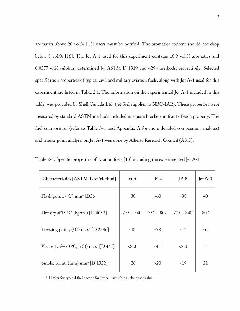
0.0577 wt% sulphur, determined by ASTM D 1319 and 4294 methods, respectively. Selected

specification properties of typical civil and military aviation fuels, along with Jet A-1 used for this

experiment are listed in Table 2.1. The information on the experimented Jet A-1 included in this

table, was provided by Shell Canada Ltd. (jet fuel supplier to NRC-IAR). These properties were

measured by standard ASTM methods included in square brackets in front of each property. The

fuel composition (refer to Table 3-1 and Appendix A for more detailed composition analyses)

and smoke point analysis on Jet A-1 was done by Alberta Research Council (ARC).

Table 2-1: Specific properties of aviation fuels [13] including the experimented Jet A-1

Characteristics [ASTM Test Method] Jet A JP-4 JP-8 Jet A-1

Flash point, (ºC) mina [D56] >38 >60 >38 40

Density @15 ºC (kg/m3) [D 4052] 775 – 840 751 – 802 775 – 840 807

Freezing point, (ºC) maxa [D 2386] -40 -58 -47 -53

Viscosity @-20 ºC, (cSt) maxa [D 445] <8.0 <8.5 <8.0 4

Smoke point, (mm) mina [D 1322] >26 >20 >19 21

a Limits for typical fuel except for Jet A-1 which has the exact value

8

Heat of combustion, the most important characteristic property of any fuel, for all these fuels

is above 42.8 MJ/kg. According to the information provided by Shell Canada on the

experimented Jet A-1, the estimated net heat of combustion (ASTM D 4529) for this fuel was

43.2 MJ/kg. Some of the fundamental properties of jet fuels are mentioned above. In addition,

some of the other significant properties are as follow:

Stability (ASTM D 3242)

A stable fuel is one whose properties remain unchanged through time (storage stability) and at

elevated temperature in the engine (thermal stability) [17].

Lubricity (ASTM D 5001)

Lubricity is a measure of liquid fuel’s effectiveness as a lubricant for reducing the friction between

solid surfaces in engine during relative motion. Jet fuel must possess a certain level of lubricity.

Volatility (ASTM D 5190 and 5191)

Volatility is important because a fuel must be vaporized before it burns. However, too high of a

volatility can result in evaporative losses.

Other properties such as non-corrosivity (ASTM D 130), cleanness (absence of water

(ASTM D 3240) and solids in fuel (ASTM D 5452)), and resistance against microbial growth in

fuel (ASTM D 6469) are also significant factors for fuels to be certified as aviation fuels

worldwide.

9

2.1.2 Proposed Alternative Jet Fuels

One of the suggested solutions in the effort to reduce the levels of GHG emissions, which has

attracted particular attention, is alternative fuels for aircrafts. According to the Air

Transportation Association (ATA), fuel is an airliner’s second largest expense. Historically, fuel

expenses have ranged from 10% – 15% of each US airline passengers’ cost, while recently it

reached as high as 35% in the third quarter of 2008 when oil prices peaked in July of that year

[18]. Fuel price instability can be detrimental to the airline industry. Alternative sources of jet

fuel might increase the price stability. However, not every alternative fuel can be employed due to

constraints specific to the use of aircraft. Sections 2.1.2.1 to 2.1.2.4 review a number of most

promising options, many of which have been experimented in this research.

2.1.2.1 Fischer-Tropsch Synthetic Kerosene

Gas-to-Liquid Process

Various carboniferous feedstocks can be converted to synthetic paraffinic kerosene (SPK)

through different synthetic fuel production processes, such as the Fischer-Tropsch (FT) process.

Fischer-Tropsch fuels are typically manufactured in a three-step process:

1) Syngas generation

The feedstock (e.g. coal, biomass or natural gas) is converted into synthetic gases (syngas) in a

few steps depending on the type of feedstock. Synthesis gas mainly consists of CO and H2.

10

2) Hydrocarbon synthesis

The syngases are catalytically converted into a mixture of C1-C40 liquid HC’s, producing

“synthetic crude”. This step is the actual FT synthesis. The general reaction dominating FT

process is,

�2n+1� H2+n COcatalyst (e.g. Ni, Co, Fe)���������������� CnH�2n+2�+n H2O �2.1�

This crude is then sent to distillation columns to separate different cuts.

3) Upgrading

The mixture of FT hydrocarbons from the distillation columns is then upgraded through

hydrotreating, hydrocracking and isomerization and finally fractionated into the desired fuels.

Natural gas (NG) is one type of feedstock for FT process. After separating methane from

the NG and mixing it with oxygen at 1,400 ºC – 1,600 ºC in a reformer, the produced syngases

undergo low-temperature FT process to produce Gas-to-Liquid (GTL) kerosene along with

liquefied petroleum gas (LPG), naphtha, diesel and base oils. Figure 2.1 summarizes the main

steps in a GTL process. Shell Ltd. has the world’s largest GTL production plant under

construction in Qatar (Pearl Project). Shell GTL Jet Fuel, also known as FT-SPK, was approved

for use in civil aviation in late September 2009 [19].

11

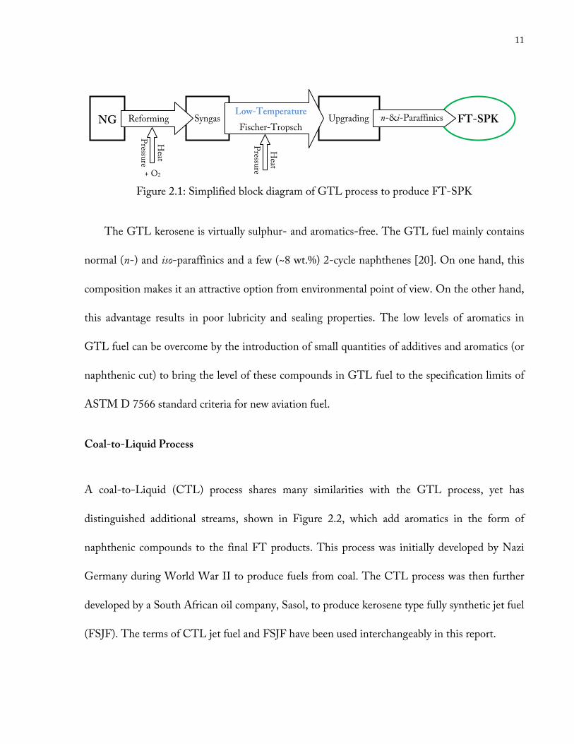
Figure 2.1: Simplified block diagram of GTL process to produce FT-SPK

The GTL kerosene is virtually sulphur- and aromatics-free. The GTL fuel mainly contains

normal (n-) and iso-paraffinics and a few (~8 wt.%) 2-cycle naphthenes [20]. On one hand, this

composition makes it an attractive option from environmental point of view. On the other hand,

this advantage results in poor lubricity and sealing properties. The low levels of aromatics in

GTL fuel can be overcome by the introduction of small quantities of additives and aromatics (or

naphthenic cut) to bring the level of these compounds in GTL fuel to the specification limits of

ASTM D 7566 standard criteria for new aviation fuel.

Coal-to-Liquid Process

A coal-to-Liquid (CTL) process shares many similarities with the GTL process, yet has

distinguished additional streams, shown in Figure 2.2, which add aromatics in the form of

naphthenic compounds to the final FT products. This process was initially developed by Nazi

Germany during World War II to produce fuels from coal. The CTL process was then further

developed by a South African oil company, Sasol, to produce kerosene type fully synthetic jet fuel

(FSJF). The terms of CTL jet fuel and FSJF have been used interchangeably in this report.

FT-SPK Upgrading

Heat

Pressure

NG Syngas Reforming

Heat

Pressure

+ O2

Low-Temperature

Fischer-Tropsch n-&i-Paraffinics

12

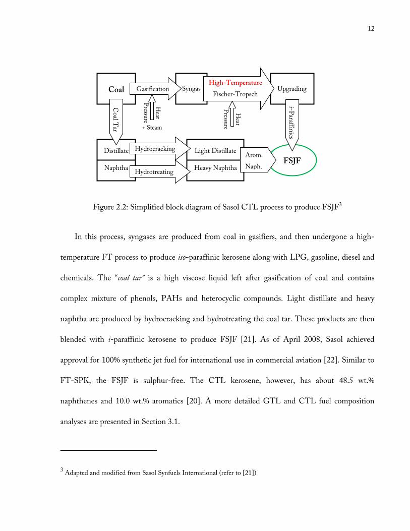
Figure 2.2: Simplified block diagram of Sasol CTL process to produce FSJF3

In this process, syngases are produced from coal in gasifiers, and then undergone a high-

temperature FT process to produce iso-paraffinic kerosene along with LPG, gasoline, diesel and

chemicals. The “coal tar” is a high viscose liquid left after gasification of coal and contains

complex mixture of phenols, PAHs and heterocyclic compounds. Light distillate and heavy

naphtha are produced by hydrocracking and hydrotreating the coal tar. These products are then

blended with i-paraffinic kerosene to produce FSJF [21]. As of April 2008, Sasol achieved

approval for 100% synthetic jet fuel for international use in commercial aviation [22]. Similar to

FT-SPK, the FSJF is sulphur-free. The CTL kerosene, however, has about 48.5 wt.%

naphthenes and 10.0 wt.% aromatics [20]. A more detailed GTL and CTL fuel composition

analyses are presented in Section 3.1.

3 Adapted and modified from Sasol Synfuels International (refer to [21])

Heat

Pressure

Heat

Pressure

+ Steam

Upgrading Coal Syngas Gasification High-Temperature

Fischer-Tropsch

FSJF

Distillate

Naphtha

Light Distillate

Heavy Naphtha Hydrotreating

Hydrocracking Arom.

Naph.

Coal T

ar

i-Paraffinics

13

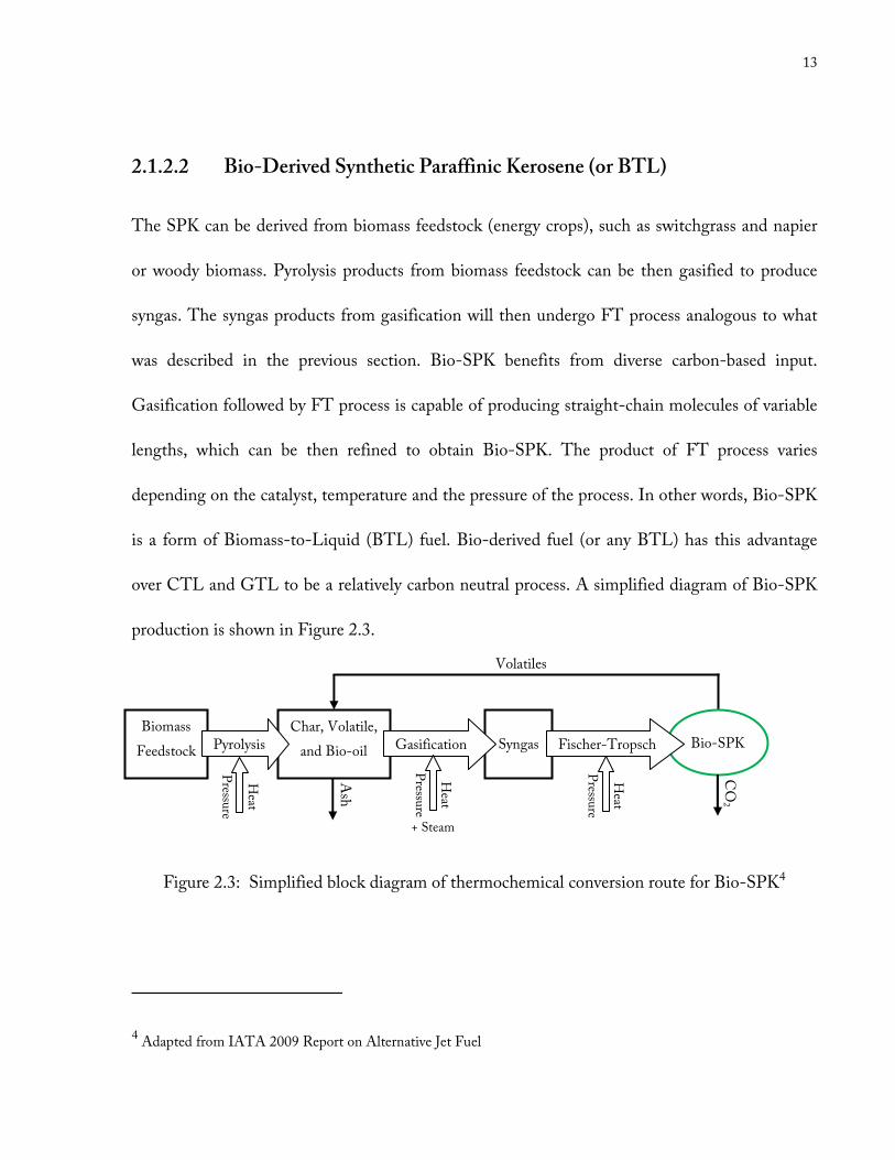
2.1.2.2 Bio-Derived Synthetic Paraffinic Kerosene (or BTL)

The SPK can be derived from biomass feedstock (energy crops), such as switchgrass and napier

or woody biomass. Pyrolysis products from biomass feedstock can be then gasified to produce

syngas. The syngas products from gasification will then undergo FT process analogous to what

was described in the previous section. Bio-SPK benefits from diverse carbon-based input.

Gasification followed by FT process is capable of producing straight-chain molecules of variable

lengths, which can be then refined to obtain Bio-SPK. The product of FT process varies

depending on the catalyst, temperature and the pressure of the process. In other words, Bio-SPK

is a form of Biomass-to-Liquid (BTL) fuel. Bio-derived fuel (or any BTL) has this advantage

over CTL and GTL to be a relatively carbon neutral process. A simplified diagram of Bio-SPK

production is shown in Figure 2.3.

Figure 2.3: Simplified block diagram of thermochemical conversion route for Bio-SPK4

4 Adapted from IATA 2009 Report on Alternative Jet Fuel

CO2

Ash

Volatiles

Bio-SPK Biomass

Feedstock

Char, Volatile,

and Bio-oil Syngas Gasification Fischer-Tropsch Pyrolysis

Heat

Pressure

Heat

Pressure

+ Steam

Heat

Pressure

14

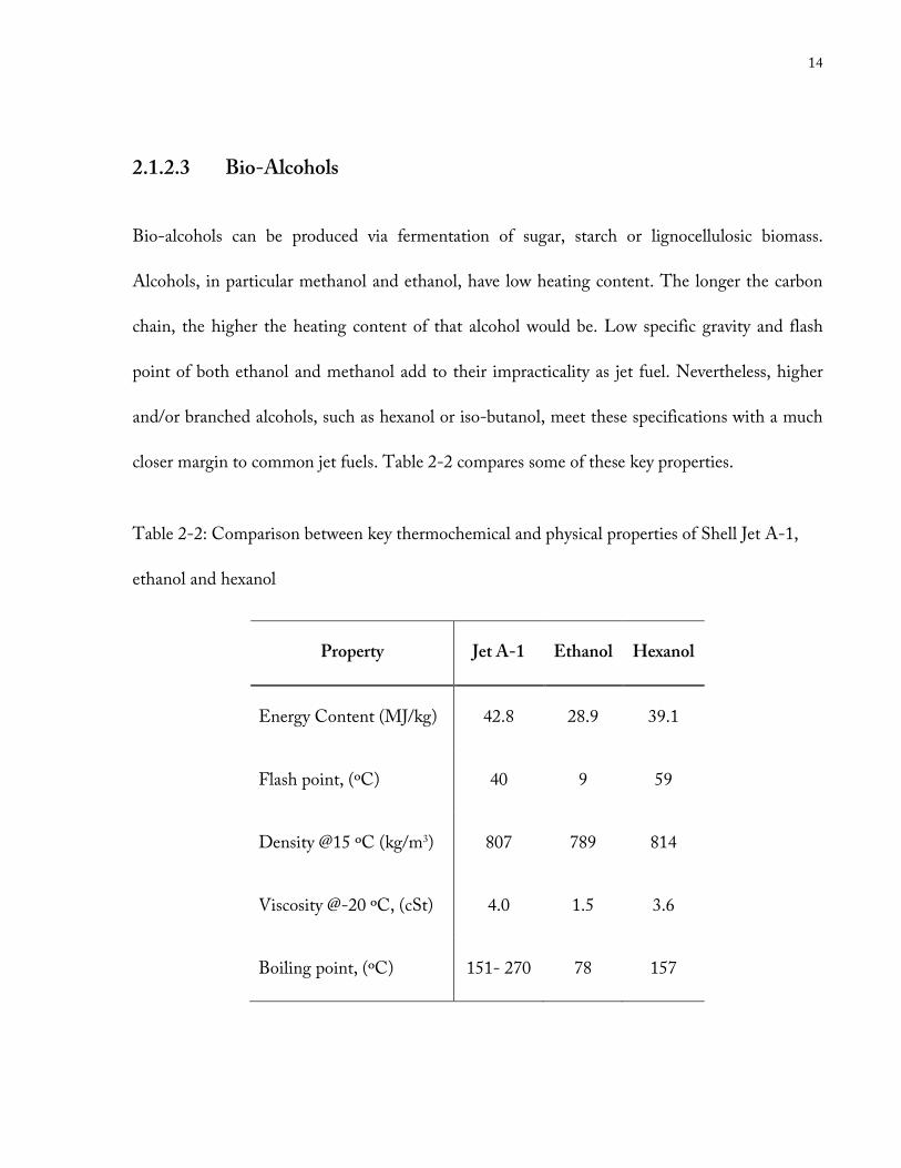
2.1.2.3 Bio-Alcohols

Bio-alcohols can be produced via fermentation of sugar, starch or lignocellulosic biomass.

Alcohols, in particular methanol and ethanol, have low heating content. The longer the carbon

chain, the higher the heating content of that alcohol would be. Low specific gravity and flash

point of both ethanol and methanol add to their impracticality as jet fuel. Nevertheless, higher

and/or branched alcohols, such as hexanol or iso-butanol, meet these specifications with a much

closer margin to common jet fuels. Table 2-2 compares some of these key properties.

Table 2-2: Comparison between key thermochemical and physical properties of Shell Jet A-1,

ethanol and hexanol

Property Jet A-1 Ethanol Hexanol

Energy Content (MJ/kg) 42.8 28.9 39.1

Flash point, (ºC) 40 9 59

Density @15 ºC (kg/m3) 807 789 814

Viscosity @-20 ºC, (cSt) 4.0 1.5 3.6

Boiling point, (ºC) 151- 270 78 157

15

There is ongoing research for developing production process of higher alcohols such as

butanol [23,24] and hexanol [25] on a commercial scale. The water solubility in alcohol,

however, poses a contamination issue. Based on the above, a higher alcohol combined with

kerosene is been recommended as a fuel. A blend of 80 vol.% GTL and 20 vol.% hexanol

(Hex20-GTL) was tested in the current study.

2.1.2.4 Other Blends

In order to avoid compromise of kerosene performance in jet engines, a blend of suggested

alternative fuels with mineral kerosene is advised. Together with the proposed blends mentioned

above (20 vol.% hexanol + 80 vol.% GTL), a fuel mixture of 50 vol.% naphthenic cut with GTL

kerosene was suggested by ALFA-BIRD program for examination as alternative jet fuel.

Naphthenic compounds are derived by liquefaction of coal or biomass [26]. Due to time

constraints, this fuel was left out of the scope of this research.

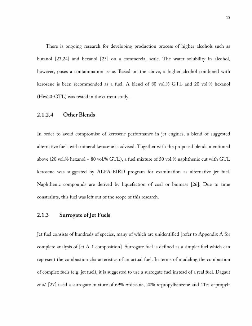
2.1.3 Surrogate of Jet Fuels

Jet fuel consists of hundreds of species, many of which are unidentified [refer to Appendix A for

complete analysis of Jet A-1 composition]. Surrogate fuel is defined as a simpler fuel which can

represent the combustion characteristics of an actual fuel. In terms of modeling the combustion

of complex fuels (e.g. jet fuel), it is suggested to use a surrogate fuel instead of a real fuel. Dagaut

et al. [27] used a surrogate mixture of 69% n-decane, 20% n-propylbenzene and 11% n-propyl-

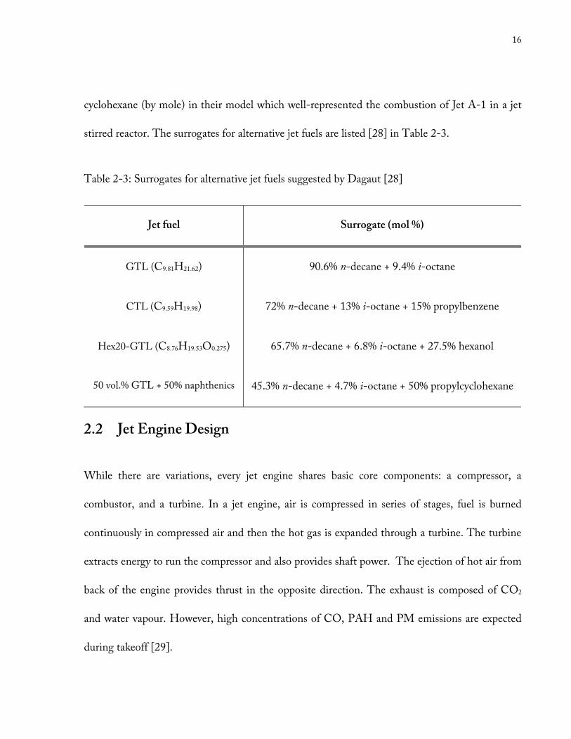
16

cyclohexane (by mole) in their model which well-represented the combustion of Jet A-1 in a jet

stirred reactor. The surrogates for alternative jet fuels are listed [28] in Table 2-3.

Table 2-3: Surrogates for alternative jet fuels suggested by Dagaut [28]

Jet fuel Surrogate (mol %)

GTL (C9.81H21.62) 90.6% n-decane + 9.4% i-octane

CTL (C9.59H19.98) 72% n-decane + 13% i-octane + 15% propylbenzene

Hex20-GTL (C8.76H19.53O0.275) 65.7% n-decane + 6.8% i-octane + 27.5% hexanol

50 vol.% GTL + 50% naphthenics 45.3% n-decane + 4.7% i-octane + 50% propylcyclohexane

2.2 Jet Engine Design

While there are variations, every jet engine shares basic core components: a compressor, a

combustor, and a turbine. In a jet engine, air is compressed in series of stages, fuel is burned

continuously in compressed air and then the hot gas is expanded through a turbine. The turbine

extracts energy to run the compressor and also provides shaft power. The ejection of hot air from

back of the engine provides thrust in the opposite direction. The exhaust is composed of CO2

and water vapour. However, high concentrations of CO, PAH and PM emissions are expected

during takeoff [29].

17

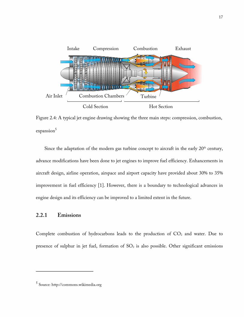
Figure 2.4: A typical jet engine drawing showing the three main steps: compression, combustion,

expansion5

Since the adaptation of the modern gas turbine concept to aircraft in the early 20th century,

advance modifications have been done to jet engines to improve fuel efficiency. Enhancements in

aircraft design, airline operation, airspace and airport capacity have provided about 30% to 35%

improvement in fuel efficiency [1]. However, there is a boundary to technological advances in

engine design and its efficiency can be improved to a limited extent in the future.

2.2.1 Emissions

Complete combustion of hydrocarbons leads to the production of CO2 and water. Due to

presence of sulphur in jet fuel, formation of SO2 is also possible. Other significant emissions

5 Source: http://commons.wikimedia.org

Intake Compression Combustion Exhaust

Air Inlet Combustion Chambers Turbine

Cold Section Hot Section

18

include CO, unburned hydrocarbon and PM which are the results of incomplete combustion,

engine design, operating conditions and/or combination of all.

Carbon dioxide is a primary GHG. Carbon monoxide, on the other hand, is highly toxic.

Sulphur oxides (mainly SO2) are known to contribute to the formation of aerosols and

particulates. These compounds are also serious respiratory health hazards, especially for children

[30]. With regards to NOX emissions, there are two sources for NOX formation in engine: (1)

from the oxidation of atmospheric nitrogen (N2) at very high temperatures found in the

combustor (thermal NOX), and (2) from fuel bound nitrogen, which in trace amount improves the

lubricity of fuel. NOX emissions are considered as central contributors in the formation of ozone

near ground level [31].

2.3 Fundamentals of Coflow Laminar Diffusion Flame

Fuel combustion is a complex process; the understanding of which requires knowledge of fuel

chemistry, thermodynamics, mass and heat transfer, reaction kinetics and fluid dynamics of the

process. A diffusion flame is a flame in which fuel and oxidant are separately introduced and the

rate of fuel consumption is determined by the diffusion rate. Examples of diffusion flames are the

candle flame, gaseous fuel jets and the Bunsen-burner flame [32].

19

Coflow flame is a conical multi-dimensional flame. Coflow flame studies have also been

used to shed light on how soot is formed in diffusion burning, for example works done by

Santoro et al. [33,34,35] and others [36,37].

Although the coflow laminar flame study appears to be far from the reality of the turbulent

phenomena happening in a jet engine at high pressures, this study is essential to fully understand

the combustion of jet fuels in any condition in detail. Turbulent combustion is far from being

fully understood. “Since the flow is turbulent in nearly all engineering applications, the urgent

need to resolve engineering problems has led to preliminary solutions called turbulence models”

[38]. Turbulent models stem from equations governing laminar flames. In both laminar and

turbulent flames, the same physical processes are applied and many turbulent flame theories are

based on underlying laminar flame structure [39]. Because measuring gaseous species in a

turbulent flame, especially in sooting flames such as jet fuel flames, is difficult, the study of

gaseous species in laminar flames is necessary to understand and validate combustion models. A

coflow laminar flame, however, gives a steady, relatively simple axisymmetric flow field and thus

makes the understanding of the flow field amenable. Knowledge of the concepts developed and

results obtained from laminar flame is a necessary prerequisite to the study of turbulent flames

[39]. This research also couples with a numerical study (refer to [11]).

20

2.3.1 Governing Equations for Laminar Diffusion Flame

Chemically reacting flow problems, such as the laminar diffusion flame are mathematically

formulated using equations for species and mass continuity, momentum and conservation of

energy. This problem is considered at a steady flow for a two-dimensional axisymmetric (r- and z-

coordinates) geometry. These series of derived equations are shown in Appendix D.

2.3.2 Flame Liftoff

The distance from the base of a detached flame to its fuel nozzle is called liftoff. A minimum

liftoff is desired to avoid heat conduction back to the burner through the fuel nozzle. In order to

avoid partial premixing, a flame liftoff should not exceed a specific height. When the flame

approaches the maximum liftoff, inhomogeneous fuel-air premixing occurs [40]. If an optimal

size of liftoff is attained, appropriate simplification can be applied to the flame’s thermal

boundary conditions. This eases and accelerates the modeling process of the flame. Further liftoff

adds to turbulence or even causes blow-off.

2.3.3 Flame Length (or Visible Flame Height)

The most common definition of flame length is the distance from the tip of the fuel nozzle (or

the burner, if they are equally levelled) to the position on the flame centreline where the fuel and

oxidizer are in a stoichiometric ratio. Based on Roper analysis for a circular fuel port [39], the

21

flame length is independent of initial velocity (fuel velocity leaving the port) or diameter

exclusively, but proportional to initial volumetric flowrate, QF.

ℒ� ≈ 38�

�������,�����

�2.2�

Here, YF, stoic is the stoichiometric mass fraction of fuel. In highly diluted system, QF is mainly

driven by diluent flowrate.

In 1928, Burke and Schumann developed set of complex equations to calculate the flame

height theoretically. Since then, several studies were done to improve the accuracy of Burke-

Schumann equations by including, for instance, buoyancy and more reasonable assumptions [41].

For the purpose of this study, however, estimating the flame height visually was found

sufficiently indicative.

22

2.4 Soot Formation in Coflow Flames

The term soot refers to nano-meter sized carbonaceous particles produced as a result of HC fuel

combustion. Numerous studies have been conducted on the hazardous effects of soot emission

on the environment and the human respiratory system. Besides direct health effects of

combustion-generated soot, the temperature decrease due to radiant heat losses from soot affects

flame length and other temperature dependent processes, such as NOX formation in engine [36].

The formation and destruction of soot is a notable feature of non-premixed flames.

Carbon molecules emit a yellow-orange light when heated. This phenomenon is called soot

luminosity. Thus, a yellow flame indicates a sooting flame, while a blue flame does not contain

soot. Considering the complex chemistry and physics of soot formation, Turns [39] has

suggested that soot formation essentially proceeds in a four-step sequence:

1) Formation of precursor species,

2) Particle inception,

3) Surface growth and particle agglomeration, and

4) Particle oxidation.

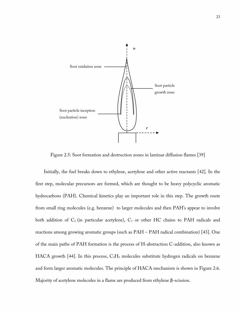
The location of these steps is shown on the next page.

23

Figure 2.5: Soot formation and destruction zones in laminar diffusion flames [39]

Initially, the fuel breaks down to ethylene, acetylene and other active reactants [42]. In the

first step, molecular precursors are formed, which are thought to be heavy polycyclic aromatic

hydrocarbons (PAH). Chemical kinetics play an important role in this step. The growth route

from small ring molecules (e.g. benzene) to larger molecules and then PAH’s appear to involve

both addition of C2 (in particular acetylene), C3 or other HC chains to PAH radicals and

reactions among growing aromatic groups (such as PAH – PAH radical combination) [43]. One

of the main paths of PAH formation is the process of H-abstraction C-addition, also known as

HACA growth [44]. In this process, C2H2 molecules substitute hydrogen radicals on benzene

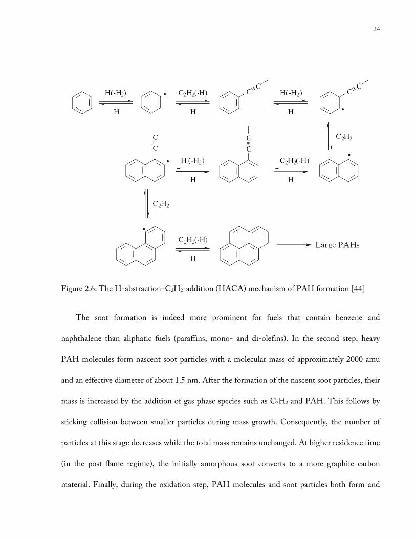
and form larger aromatic molecules. The principle of HACA mechanism is shown in Figure 2.6.

Majority of acetylene molecules in a flame are produced from ethylene β-scission.

Soot oxidation zone

Soot particle

growth zone

Soot particle inception

(nucleation) zone

z

r

24

Figure 2.6: The H-abstraction–C2H2-addition (HACA) mechanism of PAH formation [44]

The soot formation is indeed more prominent for fuels that contain benzene and

naphthalene than aliphatic fuels (paraffins, mono- and di-olefins). In the second step, heavy

PAH molecules form nascent soot particles with a molecular mass of approximately 2000 amu

and an effective diameter of about 1.5 nm. After the formation of the nascent soot particles, their

mass is increased by the addition of gas phase species such as C2H2 and PAH. This follows by

sticking collision between smaller particles during mass growth. Consequently, the number of

particles at this stage decreases while the total mass remains unchanged. At higher residence time

(in the post-flame regime), the initially amorphous soot converts to a more graphite carbon

material. Finally, during the oxidation step, PAH molecules and soot particles both form and

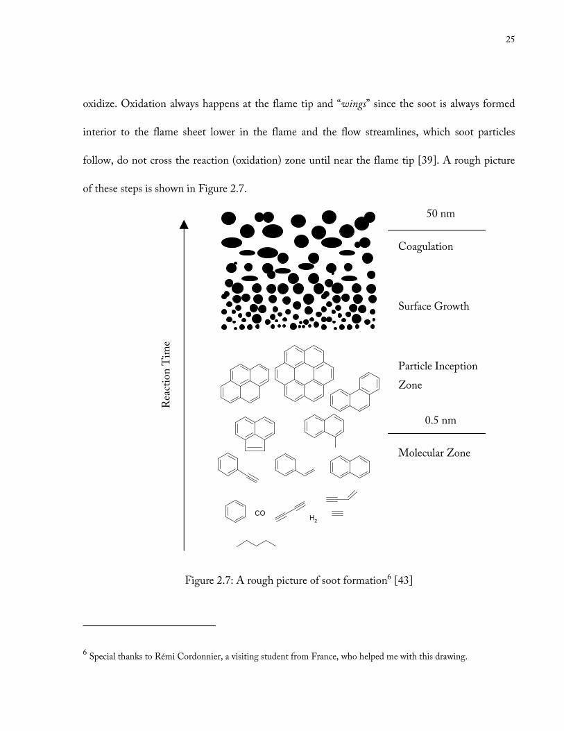
25

oxidize. Oxidation always happens at the flame tip and “wings” since the soot is always formed

interior to the flame sheet lower in the flame and the flow streamlines, which soot particles

follow, do not cross the reaction (oxidation) zone until near the flame tip [39]. A rough picture

of these steps is shown in Figure 2.7.

Figure 2.7: A rough picture of soot formation6 [43]

6 Special thanks to Rémi Cordonnier, a visiting student from France, who helped me with this drawing.

CO

CO2

O2

OH2

H2

50 nm

Coagulation

Surface Growth

Particle Inception

Zone

Reaction Time

0.5 nm

Molecular Zone

26

The formation of soot in diffusion flames can be reduced if the flame length is shortened.

Many studies have proved that fuel dilution with inert gases such as nitrogen reduces the amount

of soot [45]. Flame temperature and more importantly, the temperature field created by the

flame, influences the flame tendency to form soot considerably [42]. According to Milliken, the

cooler the flame is, the greater the tendency to soot would be [46].

Effect of Oxygen Content of Oxidizer

In coflow diffusion flames, altering the nitrogen to oxygen (O2) ratio in the oxidizer stream

changes the temperature and consequently, the soot tendency. The amount of oxygen in the

oxidizer has a strong influence on the flame length and liftoff. A small reduction in O2 content of

oxidizer stream results in longer flames and larger liftoff.

Wings

The term “wings” refers to the furthest point from centreline on the flame sheet (reactant sheet).

Smoke & Smoke Point

If some of the soot that is formed does not oxidize on its path through high-temperature

oxidizing region, soot wings may appear with the soot breaking through the flame. The soot that

breaks through is referred as smoke. Whether or not all the soot oxidizes while passing through

the oxidation zone, depends on the fuel type and flame residence time.

27

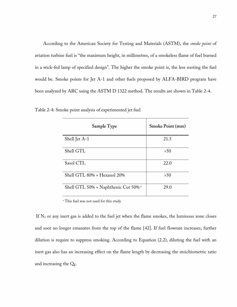
According to the American Society for Testing and Materials (ASTM), the smoke point of

aviation turbine fuel is “the maximum height, in millimetres, of a smokeless flame of fuel burned

in a wick-fed lamp of specified design”. The higher the smoke point is, the less sooting the fuel

would be. Smoke points for Jet A-1 and other fuels proposed by ALFA-BIRD program have

been analyzed by ARC using the ASTM D 1322 method. The results are shown in Table 2-4.

Table 2-4: Smoke point analysis of experimented jet fuel

Sample Type Smoke Point (mm)

Shell Jet A-1 21.5

Shell GTL >50

Sasol CTL 22.0

Shell GTL 80% + Hexanol 20% >50

Shell GTL 50% + Naphthenic Cut 50% a 29.0

a This fuel was not used for this study

If N2 or any inert gas is added to the fuel jet when the flame smokes, the luminous zone closes

and soot no longer emanates from the top of the flame [42]. If fuel flowrate increases, further

dilution is require to suppress smoking. According to Equation (2.2), diluting the fuel with an

inert gas also has an increasing effect on the flame length by decreasing the stoichiometric ratio

and increasing the QF.

28

Chapter 3

3. Experimental Apparatus & Analytical Methodology

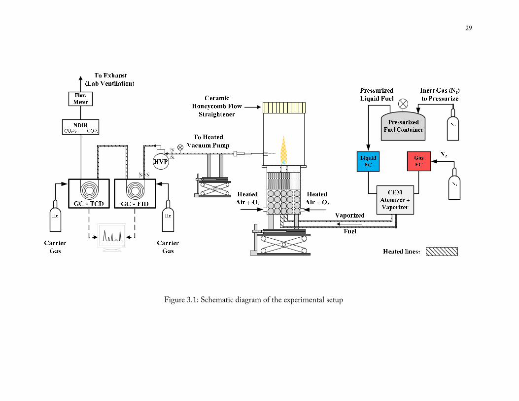
The experimental setup and analytical technique for the present study are explained in detail in

this chapter. Figure 3.1 illustrates a schematic diagram of the experimental setup. This setup was

aimed to address four different areas of interest in any coflow flame study: (1) gaseous species

analyses (scope of current research), (2) PAH measurements, (3) temperature measurement, and

(4) soot concentration and morphological properties evaluation. The process of developing this

setup can be classified to two main categories: (1) tasks that were involved with getting a stable

coflow flame from liquid fuels, (2) sections dedicated to collecting and analyzing of samples from

flames. The setup consisted of a fuel delivery system combined with a vaporizer, a coflow

diffusion flame burner, a gas sample collection system and a number of analytical equipment, all

of which were connected by heated transfer lines. Once a stable flame was achieved, gaseous

samples were continuously withdrawn from the flame to be analyzed onsite and were pumped

first to a GC-FID, and second to a GC-TCD.

29

Figure 3.1: Schematic diagram of the experimental setup

30

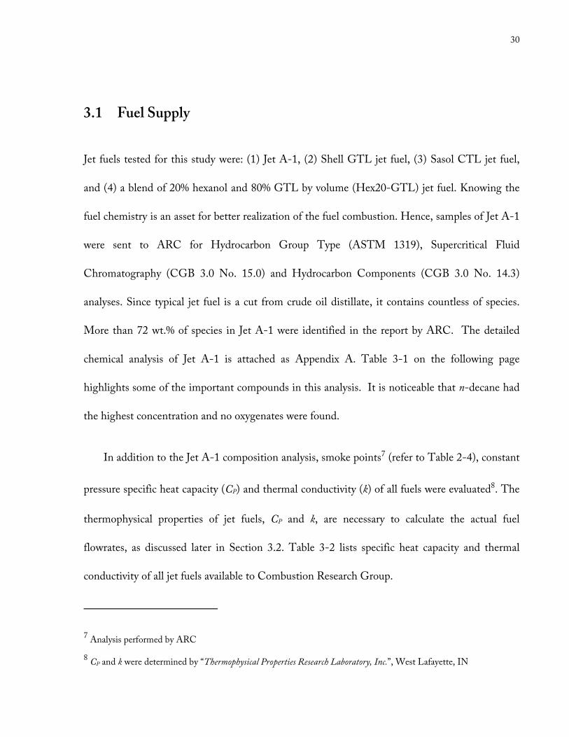
3.1 Fuel Supply

Jet fuels tested for this study were: (1) Jet A-1, (2) Shell GTL jet fuel, (3) Sasol CTL jet fuel,

and (4) a blend of 20% hexanol and 80% GTL by volume (Hex20-GTL) jet fuel. Knowing the

fuel chemistry is an asset for better realization of the fuel combustion. Hence, samples of Jet A-1

were sent to ARC for Hydrocarbon Group Type (ASTM 1319), Supercritical Fluid

Chromatography (CGB 3.0 No. 15.0) and Hydrocarbon Components (CGB 3.0 No. 14.3)

analyses. Since typical jet fuel is a cut from crude oil distillate, it contains countless of species.

More than 72 wt.% of species in Jet A-1 were identified in the report by ARC. The detailed

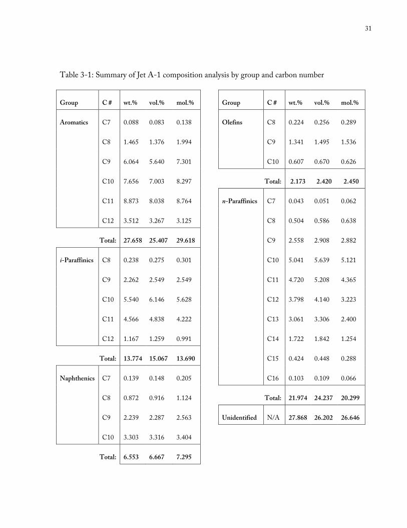
chemical analysis of Jet A-1 is attached as Appendix A. Table 3-1 on the following page

highlights some of the important compounds in this analysis. It is noticeable that n-decane had

the highest concentration and no oxygenates were found.

In addition to the Jet A-1 composition analysis, smoke points7 (refer to Table 2-4), constant

pressure specific heat capacity (CP) and thermal conductivity (k) of all fuels were evaluated8. The

thermophysical properties of jet fuels, CP and k, are necessary to calculate the actual fuel

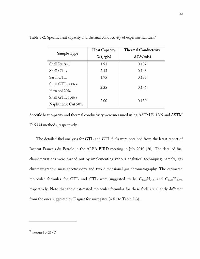
flowrates, as discussed later in Section 3.2. Table 3-2 lists specific heat capacity and thermal

conductivity of all jet fuels available to Combustion Research Group.

7 Analysis performed by ARC

8 CP and k were determined by “Thermophysical Properties Research Laboratory, Inc.”, West Lafayette, IN

31

Table 3-1: Summary of Jet A-1 composition analysis by group and carbon number

Group C # wt.% vol.% mol.% Group C # wt.% vol.% mol.%

Aromatics C7 0.088 0.083 0.138 Olefins C8 0.224 0.256 0.289

C8 1.465 1.376 1.994 C9 1.341 1.495 1.536

C9 6.064 5.640 7.301 C10 0.607 0.670 0.626

C10 7.656 7.003 8.297 Total: 2.173 2.420 2.450

C11 8.873 8.038 8.764 n-Paraffinics C7 0.043 0.051 0.062

C12 3.512 3.267 3.125 C8 0.504 0.586 0.638

Total: 27.658 25.407 29.618 C9 2.558 2.908 2.882

i-Paraffinics C8 0.238 0.275 0.301 C10 5.041 5.639 5.121

C9 2.262 2.549 2.549 C11 4.720 5.208 4.365

C10 5.540 6.146 5.628 C12 3.798 4.140 3.223

C11 4.566 4.838 4.222 C13 3.061 3.306 2.400

C12 1.167 1.259 0.991 C14 1.722 1.842 1.254

Total: 13.774 15.067 13.690 C15 0.424 0.448 0.288

Naphthenics C7 0.139 0.148 0.205 C16 0.103 0.109 0.066

C8 0.872 0.916 1.124 Total: 21.974 24.237 20.299

C9 2.239 2.287 2.563 Unidentified N/A 27.868 26.202 26.646

C10 3.303 3.316 3.404

Total: 6.553 6.667 7.295

32

Table 3-2: Specific heat capacity and thermal conductivity of experimental fuels9

Sample Type Heat Capacity

CP (J/gK)

Thermal Conductivity

k (W/mK)

Shell Jet A-1 1.91 0.137

Shell GTL 2.13 0.148

Sasol CTL 1.95 0.135

Shell GTL 80% +

Hexanol 20% 2.35 0.146

Shell GTL 50% +

Naphthenic Cut 50% 2.00 0.130

Specific heat capacity and thermal conductivity were measured using ASTM E-1269 and ASTM

D-5334 methods, respectively.

The detailed fuel analyses for GTL and CTL fuels were obtained from the latest report of

Institut Francais du Petrole in the ALFA-BIRD meeting in July 2010 [20]. The detailed fuel

characterizations were carried out by implementing various analytical techniques; namely, gas

chromatography, mass spectroscopy and two-dimensional gas chromatography. The estimated

molecular formulas for GTL and CTL were suggested to be C10.08H21.97 and C11.38H21.04,

respectively. Note that these estimated molecular formulas for these fuels are slightly different

from the ones suggested by Daguat for surrogates (refer to Table 2-3).

9 measured at 23 ºC

33

Figure 3.2: Comparison between main HC groups composition in GTL and CTL fuels

3.2 Fuel Vaporization System

Kerosene fuels are complex mixtures of HC’s with relatively high boiling points, ranging between

145 – 300 ºC. Vaporization of heavy multi-component liquid fuels, such as the fuels for the

current study, is a significant challenge. To overcome this challenge, liquid fuels were highly

diluted with nitrogen (carrier gas) and vaporized in a unique vaporization system. The nitrogen

addition not only assists the vaporization process, but also reduces the overall amount of soot.

0

5

10

15

20

25

C9 C10 C11 C12 C13 C14 C15

wt. %

C #

i-Paraffinics

CTL

GTL

0

2

4

6

8

10

12

14

C9 C10 C11 C12 C13 C14 C15

wt. %

C #

n-Paraffinics

CTL

GTL

0

0.5

1

1.5

2

2.5

C7 C8 C9 C10 C11 C12 C13 C14 C15

wt. %

C #

AromaticsCTL

GTL

0

2

4

6

8

10

C9 C10 C11 C12 C13 C14 C15 C16 C17 C18

wt. %

C #

NaphthenicsCTL

GTL

34

A Bronkhorst® Controlled Evaporator Mixer (CEM) unit10 served as the fuel delivery

system. This unit consists of a temperature-controlled vaporizer chamber, a liquid mass flow

meter with control function (LIQUI-FLOW), and a gas mass flow controller (EL-FLOW).

The temperature of CEM and mass flows were controlled by a digital readout11. The maximum

capacity of this unit is 20 g/h of liquid (fuel) and 2 L/min of carrier gas (N2) flowrates. The

CEM temperature can reach up to 200 ºC. The N2 should be supplied at inlet gauge pressures

between 235 – 305 kPa (max. 163 kPa higher than outlet pressure). The inlet gauge pressure of

liquid mass flow controller must sustain at 295 kPa. In order to maintain this pressure, fuel was

pressurized by N2 (inert gas) in a Millipore12 pressurized tank. The solubility of N2 in HC liquids

similar to jet fuels (such as n-decane and n-dodecane) was reviewed [47,48]. Henry’s Law was

not applicable at this moderately low pressure. Thus, N2 solubility in fuel was negligible. The

liquid flow meter was calibrated by the manufacture for n-tetradecane (C14H30). The flow

properties of C14H30 match with those of jet fuel to a good extent. Nonetheless, Hoskin

Scientific, the vender of CEM unit, agreed to calculate the actual liquid flowrate for any fuel,

using the four fuel properties of CP, k, � and �. The liquid mass flow meter/controller was set to

values (on C14H30 basis) which corresponded to equal mass flowrates for all the fuels (i.e.

10 W-102A-NN0-K (midsize) model

11 E-7120 model

12 1 US Gallon size

35

�� �� ! " = �� �� ! $) (see Table 3-3 on Page 39). Gas and liquid streams were mixed in a mixing

device, which includes an atomizer and a control valve, before entering the heat exchanger. The

following drawing of vaporizer setup, elaborates how the CEM units communicate and function.

Figure 3.3: Bronkhorst® liquid delivery system with vapour control

The flow sensor assembled on the top of the control valve commends the valve to maintain the

liquid flow at the setpoint value, regardless of pressure change in the mixing device. This fine-

tuned control provides an accurate liquid flow which results in a uniform vapour mixture. The

desired flow and temperature values were set by the digital readout and control system power

supplier. Temperature and flowrate setpoints were specified on the digital readout power supply.

Control Valve

To Digital

Readout Box

Controlled

Evaporator

Mixer

Atomizer

Heated

Liquid Flow Meter Gas Flow Controller

36

In order to prevent fuel condensation, vapourized fuel/N2 mixture was transferred from the

CEM vaporizer to the burner via a 1.8 m long heated transfer line13.

3.3 Coflow Diffusion Flame Burner

Coflow diffusion flames, which are radially symmetric 2-D flames, offer a great deal of

information about the combustion of sooting flames in a more realistic environment. In the

present study, a coannular burner was utilized in which different jet fuels were burned in a

mixture of air and oxygen under atmospheric pressure condition. The drawings of the coflow

burner and its section cut are shown in Figure 3.4 below.

Figure 3.4: Schematic diagram and section cut of a coflow burner (Ox: Oxidizer)

13 Custom design by Unique Heated Products Instrument Grade Heating Sample Line

Fuel + N2 mixture

Ox

Glass beads

Metal foam

Ox

Ox

Ox

37

The burner is comprised of a 10.9 mm ID steel fuel nozzle (12.7 mm OD) surrounded by an

88 mm ID (100 mm OD) outer air passage. The thickness of burner’s wall is 6 mm. Before

exiting the nozzle, the oxidizer passes through a packed bed of 5 mm diameter glass beads and a

porous metal disk to provide a uniform laminar oxidizer flow and enhance flame stability. To

avoid vapour fuel condensation along the fuel tube, the bottom part of the fuel tube was heated

using Omega heating tapes14 and the top part using thin flexible Minco heaters. The fuel nozzle

was long enough to assure a fully developed fuel/N2 mixture flow. The flame was enclosed in a

30 cm clear cylindrical Plexiglas® to protect the flame from laboratory air movement. A narrow

vertical slot was machined in the chimney to provide access for gas sampling. A 10 cm long

ceramic honey comb was mounted at the exhaust of the chimney to straighten the flow exiting

the chimney. The flow straightener enhances the flame stability dramatically. There are four

equally spaced air inlet port located at the bottom of the burner.

3.3.1 What is a Suitable Flame?

A suitable flame in this study is defined as a stable flame with the desired flame length (min.

of 5 – 6 cm), liftoff (max. ~2 mm), and proper soot concentration. Since the fuel mixture was

highly diluted with N2, the fuel jet velocity was mainly determined by the flow of diluent N2. On

the other hand, stabilization of a lifted flame is very sensitive to the coflow air [40,49]. Hence,

14 Omega® Heavy Insulated Heating Tapes (STH series), 156 W

38

different air/fuel/N2 flowrate ratios were examined to find the most “suitable” flame. It was

concluded that the addition of a small amount of O2 to the oxidizer stream is crucial in achieving

the desired flame. The addition of O2 is critical in lowering the flame liftoff and it also changes

soot luminosity, as discussed in Section 2.4.

There are two main limitations on choosing the fuel and nitrogen flowrates and in general,

the fuel/N2 ratio: a) flame height and b) soot concentration.

a) A sufficiently long flame enables a generous number of sampling points, while too long of a

flame results in a flickering flame tip and instability of the whole flame. As shown by the

Equation (2.9), the flame height is highly dependent on the fuel-diluent mixture volumetric

flowrate and fuel mole fraction.

b) The soot concentration in the flame should be such that it allows for gaseous species

sampling without clogging the microprobe, while providing a high enough extinction of the

laser beam for accurate soot volume fraction measurements.

Besides the fuel nozzle, the enriched O2 oxidizer stream was also heated. The hot oxidizer

stream prevented the fuel from forming a cloud of fuel mist after exiting the tip of the fuel nozzle

and also improves flame stability. The oxidizer stream was distributed evenly through a 4-way

manifold within the four coflow air inlets.

39

3.4 Experimental Temperature and Flow Settings

3.4.1 Flow Controls

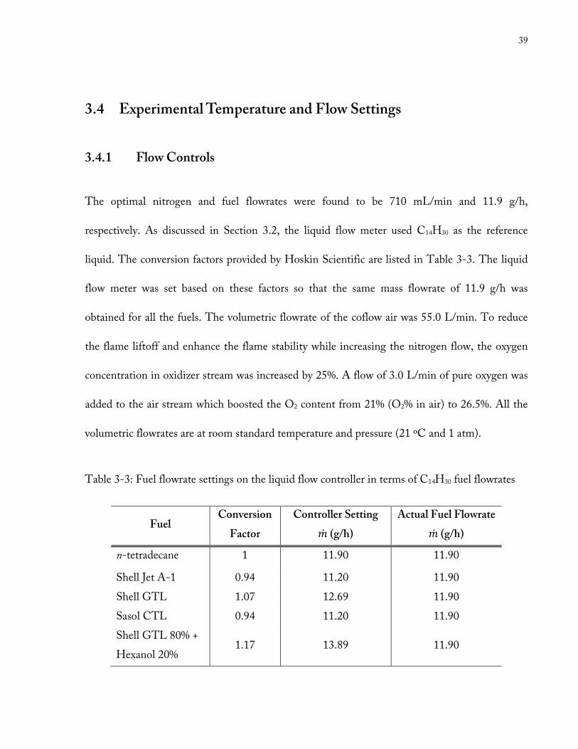
The optimal nitrogen and fuel flowrates were found to be 710 mL/min and 11.9 g/h,

respectively. As discussed in Section 3.2, the liquid flow meter used C14H30 as the reference

liquid. The conversion factors provided by Hoskin Scientific are listed in Table 3-3. The liquid

flow meter was set based on these factors so that the same mass flowrate of 11.9 g/h was

obtained for all the fuels. The volumetric flowrate of the coflow air was 55.0 L/min. To reduce

the flame liftoff and enhance the flame stability while increasing the nitrogen flow, the oxygen

concentration in oxidizer stream was increased by 25%. A flow of 3.0 L/min of pure oxygen was

added to the air stream which boosted the O2 content from 21% (O2% in air) to 26.5%. All the

volumetric flowrates are at room standard temperature and pressure (21 ºC and 1 atm).

Table 3-3: Fuel flowrate settings on the liquid flow controller in terms of C14H30 fuel flowrates

Fuel Conversion

Factor

Controller Setting

�� (g/h) Actual Fuel Flowrate

�� (g/h) n-tetradecane 1 11.90 11.90

Shell Jet A-1 0.94 11.20 11.90

Shell GTL 1.07 12.69 11.90

Sasol CTL 0.94 11.20 11.90

Shell GTL 80% +

Hexanol 20% 1.17 13.89 11.90

40

The dilution ratio for all the fuels were about 5% by mole of fuel and the remaining was

nitrogen. The sample hand calculations are attached in Appendix E.

The mean velocities of the fuel and oxidizer streams right at the exit were calculated to be

20.34 cm/s and 21.89 cm/s, respectively. The Reynold’s Number15 (Re) based on these velocities

confirmed a laminar flame (%&�� !'() = 48 and %&*�+ = 430)16 for this system.

3.4.2 Temperature Settings

The temperature of CEM vapourizer was set at 190 ºC for all the runs. The oxidizer stream was

heated to 150 ºC before entering the coflow burner. The fuel entrance tube to the burner was

kept to 210 ºC by heating tapes. The heated transfer lines were maintained at about 200 ºC,

while the fuel exit port from the vapourizer was sustained near 170 ºC with heating tapes. This

short vapourizer tube was kept at a lower temperature than other parts to avoid any damage to

the vapourizer. The output power of the heating tapes was controlled by variable voltage

transformers. The last two inches of the fuel tube, above the metal foam, was kept at 200 ºC by

Minco heaters17. The exit fuel temperature was roughly measured at around 180 ºC.

15 %& = ,�-.

16 %& ≤ 2300 is within laminar region 17 Minco heaters output power was manipulated by a DC power supply. The voltage was set to 11 V.

41

3.5 Gas Sampling System

The gas sampling system was designed in an optimal fashion to minimize the disturbance to the

flame and leakage through the transfer lines and all the units. Sampling was conducted by

continuously withdrawing gas from the flame using deactivated fused silica (FS) tubes18, typically

found in GC applications. This new design was developed by former colleague Dr. Sarathy for

collecting samples from non-sooting opposed-flow diffusion flames [50]. Minor adjustments in

its design were taken into consideration to adapt this technique for sampling from a sooting

coflow flame. The probe tips for this design are cheap and easy to replace in case of breakage or

clogging by soot. These qualities exhibit substantial advantages over old fashion quartz

microprobes, as formerly used in several flame studies [51,52]. Samples were pumped by an oil-

free, heated head, diaphragm vacuum pump19 and transferred by heated lines.

3.5.1 Sampling Apparatus

To investigate the flame chemistry accurately, reactions should be quenched at the moment

where gas is sampled. Fristrom [53] argues that rapid temperature drop is not mandatory for a

successful flame sampling. Instead, he explains how reactions halt with a large pressure drop

18 Agilent Deactivated Fused Silica Retention Gap

19 KNF oil-free heated vacuum pump Model N 036 ST. 11E (vacuum side: 24 in. Hg and pressure side: 20 psig)

42

along the probe and the destruction of the free radicals on the probe walls [54]. The discussion is

based on the fact that changes in pressure directly affects total gas density (P ∝ ρ), which is

function of mole (or mass) fraction, as shown in Equations (3.1) and (3.2). If M is used to denote

the concentration of species in a chemical reaction of nth order, the rate of reaction expression is,

2�3�24 = −6�3�7 �3.1�

where M can be written in terms of total density ρ times the mole (or mass) fraction of M, YM (or

XM). Hence, Equation (3.1) can be formulated in the following manner,

82�924 : = −6�97�7;" ∝ <7;" �3.2�

Therefore, for the 2nd order reactions, the reaction rate decreases with a decrease in pressure.

Schoenung and Hanson also showed that CO measurements in the premixed methane/air flame

were influenced by the pressure difference between the probe and sampling line [55]. In addition

to having a small orifice diameter, the probe tip must be long enough to achieve a large pressure

drop (∆P ≈ 1 atm) and destroy the free active radicals. For each experiment, an approximately

6.4 cm (2.5") long probe was cut from a 10 m long source, using a diamond cutter knife. This

length provides enough pressure drop along the probe. These fused silica microtubes are coated

with a polyimide (graphite-reinforced composite) resin on the outside to provide flexibility and

improve sealing. The coating on the microprobe tip quickly burns off once it is exposed to high

temperatures in a flame. The uncoated probe tip is quite brittle. The most suitable probe size,

43

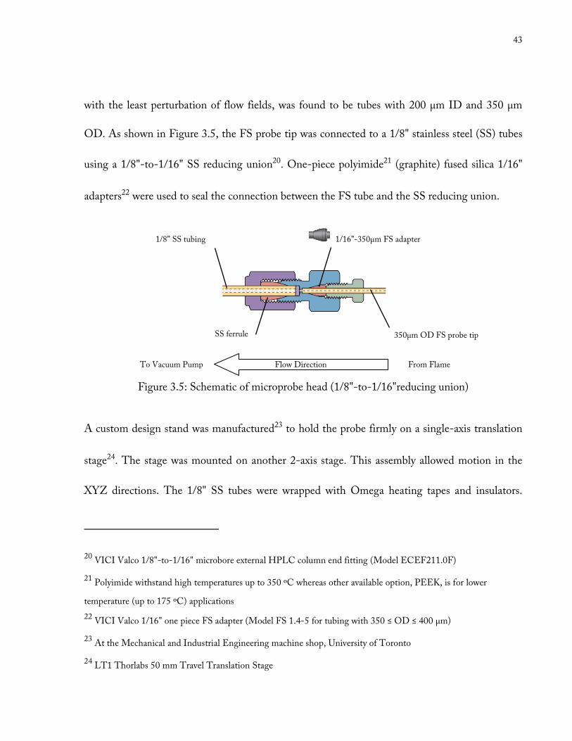
with the least perturbation of flow fields, was found to be tubes with 200 µm ID and 350 µm

OD. As shown in Figure 3.5, the FS probe tip was connected to a 1/8" stainless steel (SS) tubes

using a 1/8"-to-1/16" SS reducing union20. One-piece polyimide21 (graphite) fused silica 1/16"

adapters22 were used to seal the connection between the FS tube and the SS reducing union.

Figure 3.5: Schematic of microprobe head (1/8"-to-1/16"reducing union)

A custom design stand was manufactured23 to hold the probe firmly on a single-axis translation

stage24. The stage was mounted on another 2-axis stage. This assembly allowed motion in the

XYZ directions. The 1/8" SS tubes were wrapped with Omega heating tapes and insulators.

20 VICI Valco 1/8"-to-1/16" microbore external HPLC column end fitting (Model ECEF211.0F)

21 Polyimide withstand high temperatures up to 350 ºC whereas other available option, PEEK, is for lower

temperature (up to 175 ºC) applications

22 VICI Valco 1/16" one piece FS adapter (Model FS 1.4-5 for tubing with 350 ≤ OD ≤ 400 µm)

23 At the Mechanical and Industrial Engineering machine shop, University of Toronto

24 LT1 Thorlabs 50 mm Travel Translation Stage

1/16”-350µm FS adapter 1/8” SS tubing

SS ferrule 350µm OD FS probe tip

Flow Direction From Flame To Vacuum Pump

44

The tubes were then connected to a 1/8", 8-ft long SS heated transfer line. The temperature of

transfer line was set at 210 ºC. The pressure of the line was monitored by a vacuum gauge placed

before the pump (on the vacuum side). Between the pressure gauge and the pump, a filter25 was

arranged to collect the fine particles (≥15 µm diameter soot particles), which were carried along

with sample from the flame, to prevent any damage to the pump and downstream instrument. A

high-temperature two-way ball valve was used between the filter and the pressure gauge to shut

off the line when needed (e.g. while checking for leakage). All the lines, from the heated transfer

line, to the pump, and from the pump, to the GC-FID, were heated by several heating tapes to

prevent fuel condensation, especially in the filter.

3.5.2 Sampling Procedure

To assure repeatability of the measurements, a precise sampling procedure was established to be

performed step-by-step throughout each experiment. Prior to sampling, the pump should be

warmed up at least 30 minutes.

3.5.2.1 Detecting the Leaks

Detecting and eliminating leaks in the sampling line is the most critical step in preparing for a

successful flame sampling. A leak from ambient air into the lines will dilute the collected sample

25 Model SS-4TF-15; sintered with nominal pore size of 15µm

45

gas and will result in lower species concentrations (particularly for those species identified on the

TCD). To prevent any leakage into the system, the following practice is advised.

Before inserting the FS tube into the front of probe, the front opening of the reducing union

was capped with a SS plug. The pump, which was turned on beforehand, then immediately

creates a vacuum in the line from the tip of probe (plugged) to the pump. At this point, the

pressure gauge should show the vacuum pressure of about 81 kPa (24 in. Hg), which is the

maximum possible vacuum pressure produced by the pump. Since suction side was heated, the

pressure might drop slightly below 81 kPa (~85 kPa). Next, the ball valve was closed and pump

was turned off to check for any major leakage(s). If a rapid change in the pressure was observed,

there must have been a major leakage (more than 10 sccm) in the line; otherwise, the line can be

checked for a minor leak (less than 10 sccm). Major leaks into the sampling line were detected

using a container filled with dry ice (i.e. solidified CO2) and a few drops of water (to expedite

CO2 sublimation). The container was placed near suspected leakage points (e.g. connections) for

several minutes. Unless a spike of CO2 was detected by NDIR analyzer downstream (see Section

3.6.2) at any point, this would indicate that there was not a major leak present in the sampling

line. If no major leak was observed, the flowrate at the end of the line was checked (see Figure

3.1). When the flow meter showed an absolute zero (0.0 sccm), the sampling probe and the

transfer line were considered leak-free and ready for the next step: centring. After an already

prepared FS tube was inserted into the probe, the tip of the tube was plugged and flow was

checked to assure no leak was caused by insertion of the FS tube.

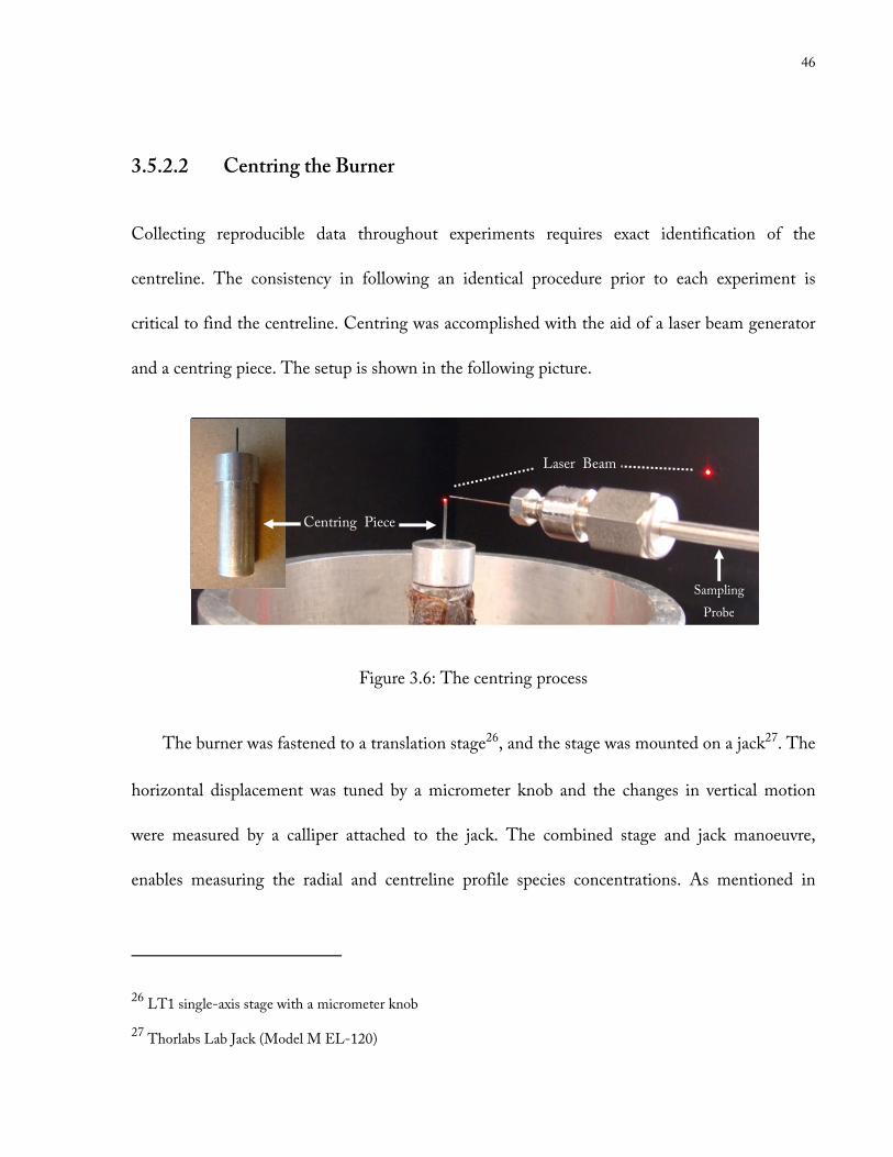
46

3.5.2.2 Centring the Burner

Collecting reproducible data throughout experiments requires exact identification of the

centreline. The consistency in following an identical procedure prior to each experiment is

critical to find the centreline. Centring was accomplished with the aid of a laser beam generator

and a centring piece. The setup is shown in the following picture.

Figure 3.6: The centring process

The burner was fastened to a translation stage26, and the stage was mounted on a jack27. The

horizontal displacement was tuned by a micrometer knob and the changes in vertical motion

were measured by a calliper attached to the jack. The combined stage and jack manoeuvre,

enables measuring the radial and centreline profile species concentrations. As mentioned in

26 LT1 single-axis stage with a micrometer knob

27 Thorlabs Lab Jack (Model M EL-120)

Centring Piece

Sampling

Probe

Laser Beam

47

Section 3.5.1, the probe could move along the XYZ axes. Prior to getting a flame, the centring

piece was inserted into the opening of the fuel nozzle. Upon shining the laser over the burner, a

bright red dot appeared on the screen opposite to the laser. The burner, jointly with the centring

piece, was brought up to the point whereby the tip of the centring piece just covered the laser

point. Every precaution was taken to place the tip of the microprobe exactly on the top of

centring piece tip perpendicularly. Since the centre of the burner was essentially fixed visually,

human eye error was inevitable. To verify that the position of the probe was centred correctly,

the flame was generated while the probe should have already been at or adjacent to the

centreline. A number of CO and CO2 measurements were taken in the neighbourhood of

initially-estimated centre, by moving the burner in horizontal direction in small increments (e.g.

0.05 mm steps). At the same height, hypothetically, the minimum CO and CO2 (or any other

species) concentrations should occur at the centre of the flame sheet. The domain of this

adjustment usually did not go beyond ±0.5 mm of the initial position determined by laser. The

CO and CO2 measurements were done by TCD instead of NDIR, due to low sensitivity of the

NDIR (see Sections 3.6.1.1 and 3.6.2).

3.5.2.3 Sampling the Flame

Majority of the previous two steps in sampling procedure were done before a flame was lit. Once

the flame was generated, the sampling probe was inserted back into the flame. Having centred

the burner, the probe remained stationary during the experiment and instead the burner was

48

moved vertically and/or horizontally. As described in the previous section, preliminary

measurements were critical to verify the centreline location. It is recommended to start sampling

from mid-low section of the flame for two main reasons: (1) the upper region of the flame may

be highly sooting and result in fast clogging of the probe, and (2) too low in the flame contains

excessive amount of unburned fuel which can saturate the FID. Therefore, the starting point was

selected at either 16 mm or 14 mm above the fuel nozzle, depending on the type of the flame

and then throughout the experiment the burner was moved downward or if possible upward (for

z ≤14 mm).

Once a stable flame was obtained and the flame temperature field reached a steady state, the

heated vacuum pump was turned on and gases withdrawn from the flame continuously. The

heated sample line was flushed for at least 40 mins before the first run. The samples traveled

from the flame, passed through the heated vacuum pump and sent to the analyzer section. On

the way out to the ventilation, exhaust flow is measured by a gas flow meter28. The exhaust

flow29 was monitored to capture clogging or otherwise observe the flow trends at each point in

the flame. The lower in the flame, the lower the temperature, and consequently the higher the

gas density is. The flowrate is known to be a function of gas density. As the probe distanced from

28 Humonics Veri-Flow 500 Electronic Flow meter

29 Note that this flow could be lower than actual suction flowrate due to leaks in the line after the pump. However, a

relative flow is of the significance for the purpose of this study.

49

the fuel port (i.e. towards tip of the flame), the flowrate decreased from about 70 sccm in the

lower region, to less than 10 sccm at the maximum point of sampling. Another reason for this

drop in sampling flowrate was the increase in soot concentration and its coagulation at the probe

tip. The latter rationale, however, was dominating closer to the luminous region rather than

lower regions in the flame. As a result, the sampling and purge time varied depending on the

location of the probe in the flame. Lower in the flame, sampling points required short purge

times of about 5 – 10 minutes. In contrast, closer to the tip of the flame at least 40 – 50 minutes

were required to purge the line prior to sampling.

The burner’s position was adjusted with an accuracy of 0.01 mm in both vertical and

horizontal directions. Typically, a 2 mm vertical and 0.5 mm horizontal spacings were used

between each data point. More data points were chosen when further investigation was

necessary. The horizontal spacing was smaller than the vertical one due to sharper radial

concentration changes compared to the centreline profile.

The sampling process for sooting flames (e.g. CTL flame) was more challenging than a less

sooting flame (e.g. GTL flame). The effort to burn the soot mass accumulated on the tip of the

probe using a propane torch was unsuccessful. Larger probe size (320 µm ID) was also tested

with the hope to increase the sample collection time for sooting regions before clogging. Yet, not

only did the probe clog quickly, but it also disturbed the flame structure considerably (shortened

the flame length by extracting large amount of fuel).

50

3.6 Analytical Techniques

To analyze flame samples, a GC-FID was tied in series to a GC-TCD, followed by an NDIR

spectrometer. This set of analytical devices enabled us to measure C1 – C6 hydrocarbons, carbon

dioxide, carbon monoxide, oxygen and some oxygenated compounds.

3.6.1 Principles of Gas Chromatography

Gas chromatography is a technique used to separate compounds based on their differences in the

interactions with a flowing mobile phase (carrier gas) and a stationary phase (separation column). The

mobile phase carries the mixture of interest through a separation column in a controlled manner. Because

of the differences in interaction between the mixture’s components with both phases, the mobile phase

convey components at different rates, so they are retained on column for different times [56]. This

selective separation is known as partitioning. Usually, larger HC molecules arrive later to the end of the

column compared to the lighter ones. The amount of time that a given component spends in the

separation column is called the retention time (RT). To determine the RT for each component, detectors

are used at the end of column. A plot of detector response, which is in form of peaks versus time, is called

a chromatogram. Besides the RT, the size of the response peak can be obtained from a chromatogram.

The area underneath each peak corresponds to the concentration of that specific compound. The sharper

the peak, the better the separation is. Partitioning strongly depends on temperature. Therefore, for a

better separation, carrier gas passes through a separation column placed in a temperature controlled oven.

Separation of a sample with a range of boiling points is achieved by starting at a low temperature and then

increasing the temperature until less volatile compounds are eluted. Calibration gases are used as a

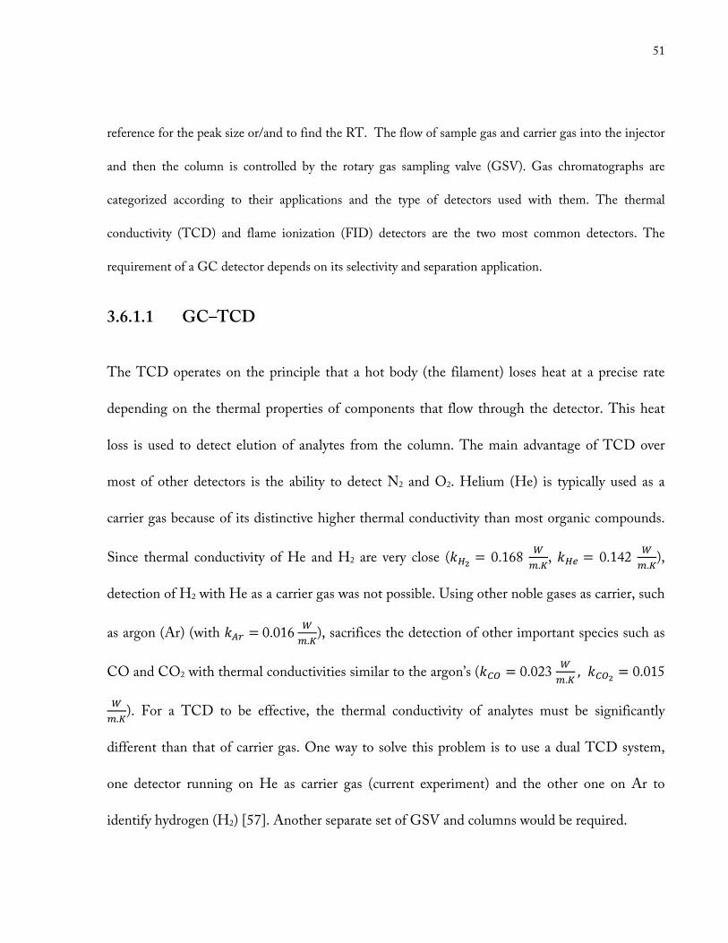
51

reference for the peak size or/and to find the RT. The flow of sample gas and carrier gas into the injector

and then the column is controlled by the rotary gas sampling valve (GSV). Gas chromatographs are

categorized according to their applications and the type of detectors used with them. The thermal

conductivity (TCD) and flame ionization (FID) detectors are the two most common detectors. The

requirement of a GC detector depends on its selectivity and separation application.

3.6.1.1 GC–TCD

The TCD operates on the principle that a hot body (the filament) loses heat at a precise rate

depending on the thermal properties of components that flow through the detector. This heat

loss is used to detect elution of analytes from the column. The main advantage of TCD over

most of other detectors is the ability to detect N2 and O2. Helium (He) is typically used as a

carrier gas because of its distinctive higher thermal conductivity than most organic compounds.

Since thermal conductivity of He and H2 are very close (6=) = 0.168 >?.@, 6= = 0.142 >

?.@),

detection of H2 with He as a carrier gas was not possible. Using other noble gases as carrier, such

as argon (Ar) (with 6A+ = 0.016 >?.@), sacrifices the detection of other important species such as

CO and CO2 with thermal conductivities similar to the argon’s (6BC = 0.023 >?.@ , 6BC) = 0.015

>?.@). For a TCD to be effective, the thermal conductivity of analytes must be significantly

different than that of carrier gas. One way to solve this problem is to use a dual TCD system,

one detector running on He as carrier gas (current experiment) and the other one on Ar to

identify hydrogen (H2) [57]. Another separate set of GSV and columns would be required.

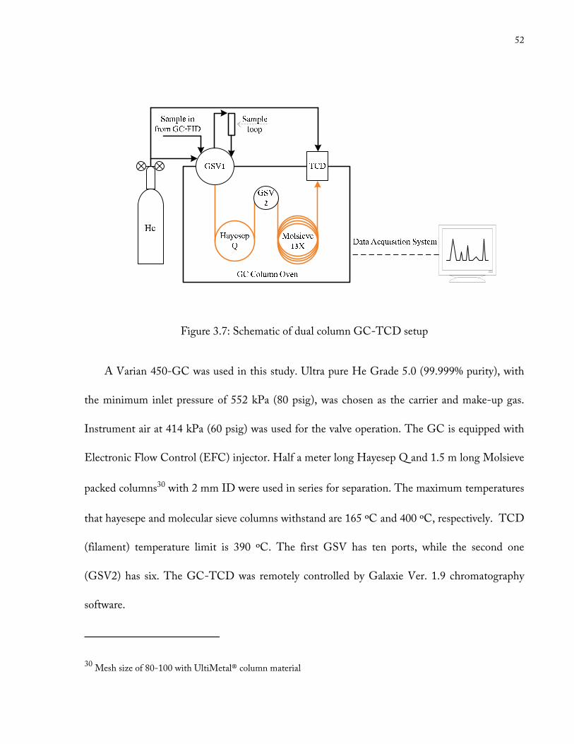
52

Figure 3.7: Schematic of dual column GC-TCD setup

A Varian 450-GC was used in this study. Ultra pure He Grade 5.0 (99.999% purity), with

the minimum inlet pressure of 552 kPa (80 psig), was chosen as the carrier and make-up gas.

Instrument air at 414 kPa (60 psig) was used for the valve operation. The GC is equipped with

Electronic Flow Control (EFC) injector. Half a meter long Hayesep Q and 1.5 m long Molsieve

packed columns30 with 2 mm ID were used in series for separation. The maximum temperatures

that hayesepe and molecular sieve columns withstand are 165 ºC and 400 ºC, respectively. TCD

(filament) temperature limit is 390 ºC. The first GSV has ten ports, while the second one

(GSV2) has six. The GC-TCD was remotely controlled by Galaxie Ver. 1.9 chromatography

software.

30 Mesh size of 80-100 with UltiMetal® column material

53

Method and Oven Temperature Profile

Detailed drawings of gas analyzing steps of the GC-TCD are included in Appendix B. Samples

continuously flowed through a 1 mL sample loop and bypassed the columns to the ventilation.

The filament was fixed at 300 ºC. Once flame sample was injected, the column oven was kept at

an initial temperature of 50 ºC for 10.0 minutes. Then the temperature was increased with the

rate of 8 ºC/min for 5.0 minutes and held for one minute at the final temperature of 90 ºC.

Upon sample injection, analyte was swept with the carrier gas onto the pre-column. Lighter

molecules such as O2, N2, CH4, and CO were trapped on the molecular sieve column while CO2

and C2-isomers were directly sent to the TCD. In the final stage, smaller molecules on molsieve

column (O2, CO, etc.) were eluted. Consequently, CO2, C2H2 and C2H4 peaks showed up first

on chromatogram (see sample chromatogram of GC-TCD in Appendix C). Other peaks (i.e.

O2, N2, CH4 and CO peaks) eluted after 10 minutes when temperature of the oven rose.

3.6.1.2 GC–FID

The FID employs an ionization detection method. In an FID, organic compounds are burned in

a tiny H2/air flame. Ions generated are then attracted to a collector plate, which produces a

current depending on type and quantity of ions. In general, FID uses capillary columns and has a

higher detection limit (more sensitive) than TCD. The FIDs are insensitive to water, CO, CO2,

and NOX.

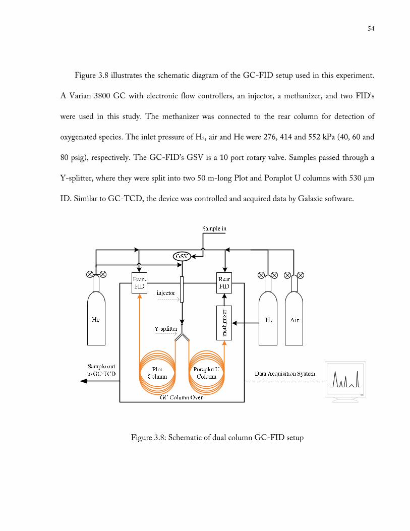
54

Figure 3.8 illustrates the schematic diagram of the GC-FID setup used in this experiment.

A Varian 3800 GC with electronic flow controllers, an injector, a methanizer, and two FID’s

were used in this study. The methanizer was connected to the rear column for detection of

oxygenated species. The inlet pressure of H2, air and He were 276, 414 and 552 kPa (40, 60 and

80 psig), respectively. The GC-FID’s GSV is a 10 port rotary valve. Samples passed through a

Y-splitter, where they were split into two 50 m-long Plot and Poraplot U columns with 530 µm

ID. Similar to GC-TCD, the device was controlled and acquired data by Galaxie software.

Figure 3.8: Schematic of dual column GC-FID setup

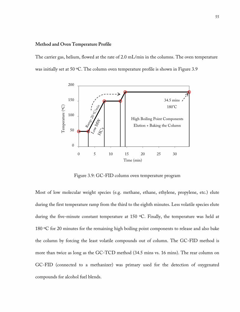
55

Method and Oven Temperature Profile

The carrier gas, helium, flowed at the rate of 2.0 mL/min in the columns. The oven temperature

was initially set at 50 ºC. The column oven temperature profile is shown in Figure 3.9

Figure 3.9: GC-FID column oven temperature program

Most of low molecular weight species (e.g. methane, ethane, ethylene, propylene, etc.) elute

during the first temperature ramp from the third to the eighth minutes. Less volatile species elute

during the five-minute constant temperature at 150 ºC. Finally, the temperature was held at

180 ºC for 20 minutes for the remaining high boiling point components to release and also bake

the column by forcing the least volatile compounds out of column. The GC-FID method is

more than twice as long as the GC-TCD method (34.5 mins vs. 16 mins). The rear column on

GC-FID (connected to a methanizer) was primary used for the detection of oxygenated

compounds for alcohol fuel blends.

0

50

100

150

200

0 5 10 15 20 25 30

Temperature (ºC)

Time (min)

High Boiling Point Components

Elution + Baking the Column

34.5 mins

180°C

56

3.6.1.3 Calibration of Gas Chromatography

Most of GC measurements were calibrated using calibration gases from Scotty® Specialty

Gases31. Calibrations were performed by flowing calibration gases at the average flowrate of the

flame sampling (approximately 50 sccm) directly into the GC sample loop. The GCs’ operating

conditions during calibration were the same as the conditions during sampling species from the

flame. A full set of calibration for all gases was performed each time prior to new fuel being

tested.

CO, CO2 and O2

A mixture of 0.5% CO, CO2, O2 and H2 was used for calibration of the lower concentrations of

CO, CO2 and O2 on the GC-TCD. Linde calibration gas containing a 10% CO and CO2

mixture was used for higher range of CO and CO2 levels. Note that the FID-methanizer can be

used for detecting low concentrations (ppm level) of CO and CO2 where TCD is not applicable.

Non-Oxygenated Hydrocarbons

A mixture of 1000 ppm C1 – C6 alkanes (methane, ethane, propane, n-butane, n-pentane, n-

hexane), C1 – C6 alkenes (ethylene, propylene, 1-butene, 1-pentene and 1-hexene) and acetylene

were used to calibrate these species on GC-FID. Some other alkynes, i.e. methylacetylene

31 48 Liters @ 300 psig, 21 ºC in balance of nitrogen

57

(propyne), 2-butyne and 1-butyne (also acetylene) were calibrated at the lower concentration of

15 ppm. Benzene was calibrated using a calibration tank containing 100 ppm of benzene in

balance of air.

Oxygenated Hydrocarbons

In addition to the above molecules, the GC-FID was calibrated for two important oxygenated

hydrocarbons in combustion: formaldehyde (CH2O) and acetaldehyde (C2H4O). These two

compounds should theoretically be present in Hex20-GTL flame in larger concentrations than

any other flame. Since these compounds are highly reactive and susceptible to rapid degradation,

using calibration gas cylinders is not a reliable method. In the current study, permeation tube

devices were used for calibration. The schematic diagram of a permeation tube device is displayed

below.

Figure 3.10: Permeation tube setup

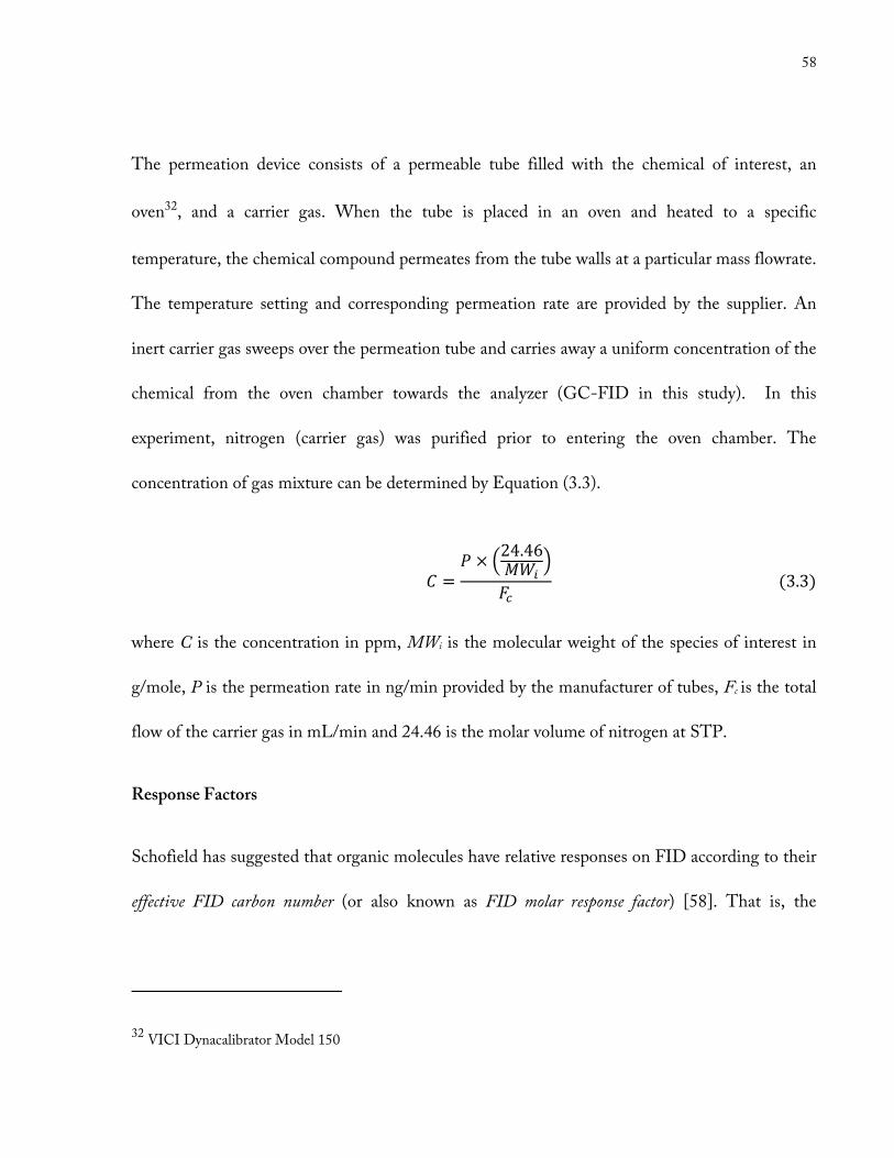
58

The permeation device consists of a permeable tube filled with the chemical of interest, an

oven32, and a carrier gas. When the tube is placed in an oven and heated to a specific

temperature, the chemical compound permeates from the tube walls at a particular mass flowrate.

The temperature setting and corresponding permeation rate are provided by the supplier. An

inert carrier gas sweeps over the permeation tube and carries away a uniform concentration of the

chemical from the oven chamber towards the analyzer (GC-FID in this study). In this

experiment, nitrogen (carrier gas) was purified prior to entering the oven chamber. The

concentration of gas mixture can be determined by Equation (3.3).

D =< × F24.46

3I� JK�

�3.3�

where C is the concentration in ppm, MWi is the molecular weight of the species of interest in

g/mole, P is the permeation rate in ng/min provided by the manufacturer of tubes, Fc is the total

flow of the carrier gas in mL/min and 24.46 is the molar volume of nitrogen at STP.

Response Factors

Schofield has suggested that organic molecules have relative responses on FID according to their

effective FID carbon number (or also known as FID molar response factor) [58]. That is, the

32 VICI Dynacalibrator Model 150

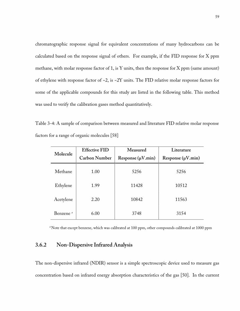
59

chromatographic response signal for equivalent concentrations of many hydrocarbons can be

calculated based on the response signal of others. For example, if the FID response for X ppm

methane, with molar response factor of 1, is Y units, then the response for X ppm (same amount)

of ethylene with response factor of ~2, is ~2Y units. The FID relative molar response factors for

some of the applicable compounds for this study are listed in the following table. This method

was used to verify the calibration gases method quantitatively.

Table 3-4: A sample of comparison between measured and literature FID relative molar response

factors for a range of organic molecules [58]

Molecule Effective FID

Carbon Number

Measured

Response (µV.min)

Literature

Response (µV.min)

Methane 1.00 5256 5256

Ethylene 1.99 11428 10512

Acetylene 2.20 10842 11563

Benzene a 6.00 3748 3154

a Note that except benzene, which was calibrated at 100 ppm, other compounds calibrated at 1000 ppm

3.6.2 Non-Dispersive Infrared Analysis

The non-dispersive infrared (NDIR) sensor is a simple spectroscopic device used to measure gas

concentration based on infrared energy absorption characteristics of the gas [50]. In the current

60

study, the NDIR33 instrument was primarily exercised for the diagnosis of the steady state, based

on CO and CO2 concentration changes. It was zeroed each time prior to the experiment and

calibrated using a Linde 10% CO and CO2 mixture for the high range and a 0.5% Scotty gas for

the low range. The readouts for both high and low levels of CO and CO2 percentages are located

on the front panel of the device. NDIR was connected downstream from the GC-TCD and

before the sample exited to the ventilation. A water-bath cooling system and a filter were

implemented midway between GC-TCD and NDIR to remove condensed fuel from the gases.

The NDIR measurements are helpful for real-time analyses, yet, very crude assessment. For

instance, for centring the burner, which data points are only 0.1 mm apart from each other, GC-

TCD had to be used for sensitive comparisons between measurements, even though it took

much longer time to accomplish the centring task. The NDIR diagnosis, on the other hand,

provided sufficiently accurate information on whether steady state was reached. Upon changing

the sampling location (by moving the burner), it took between 5 to 45 minutes for the NDIR to

stabilize, depending on the probe location. Based on the previous discussion in Section 3.5.2.3,

as suction flowrates decreases for sampling points higher up in the flame, longer transition times

were perceived. A minimum time of 40 – 50 minutes was required to achieve steady state in

many cases where the flames were highly sooting (e.g. CTL and Jet A-1 flames).

33 NOVA NDIR Analyzer Model 7800P2A

61

Chapter 4

4. Results & Discussions

The primary goal of this study is to measure the gaseous species in coflow diffusion flames for

conventional and alternative jet fuels. The species profiles of these fuels are compared in this

chapter. The sampling analyses were carried out by gas chromatography and major species that

were identified included but not limited to carbon monoxide, carbon dioxide, oxygen, methane,

ethane (C2H6), ethylene (C2H4), propylene (C3H6), and acetylene (C2H2). For a number of fuels,

the concentration of other species, such as benzene (C6H6), propyne (C3H4), and 1-butene

(C4H8) were also reported. The GTL-hexanol blend flame was investigated for the presence of

acetaldehyde and formaldehyde. A few other species (e.g. propane, n-hexane or 2-butyne) were

identified but not reported because either they were below the limit of detection (LOD) or limit

of quantification (LOQ). Some of the lighter HC’s such as, CH4 and C2-isomers, can be

identified on both FID and TCD. Since the FID is more sensitive and accurate, measurements

determined by GC-FID were reported in this study. Both response factors and calibration gas

methods produced close results (within ±10%). The calibration gas method, however, was

preferred as the standard method of calibration for this study. Each experiment was repeated for

a minimum of three times. Since the results were reproducible within ±15%, the measured values

for each data point were averaged over the trials. The outliners are also reported separately.

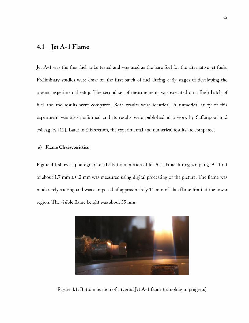
62

4.1 Jet A-1 Flame

Jet A-1 was the first fuel to be tested and was used as the base fuel for the alternative jet fuels.

Preliminary studies were done on the first batch of fuel during early stages of developing the

present experimental setup. The second set of measurements was executed on a fresh batch of

fuel and the results were compared. Both results were identical. A numerical study of this

experiment was also performed and its results were published in a work by Saffaripour and

colleagues [11]. Later in this section, the experimental and numerical results are compared.

a) Flame Characteristics

Figure 4.1 shows a photograph of the bottom portion of Jet A-1 flame during sampling. A liftoff

of about 1.7 mm ± 0.2 mm was measured using digital processing of the picture. The flame was

moderately sooting and was composed of approximately 11 mm of blue flame front at the lower

region. The visible flame height was about 55 mm.

Figure 4.1: Bottom portion of a typical Jet A-1 flame (sampling in progress)

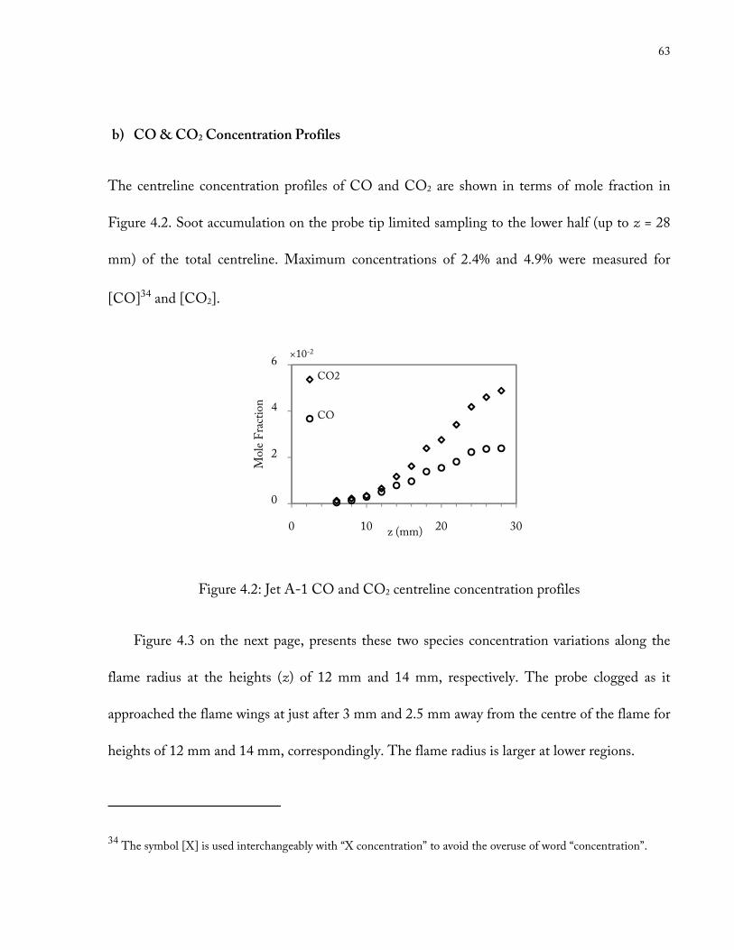
63

b) CO & CO2 Concentration Profiles

The centreline concentration profiles of CO and CO2 are shown in terms of mole fraction in

Figure 4.2. Soot accumulation on the probe tip limited sampling to the lower half (up to z = 28

mm) of the total centreline. Maximum concentrations of 2.4% and 4.9% were measured for

[CO]34 and [CO2].

Figure 4.2: Jet A-1 CO and CO2 centreline concentration profiles

Figure 4.3 on the next page, presents these two species concentration variations along the

flame radius at the heights (z) of 12 mm and 14 mm, respectively. The probe clogged as it

approached the flame wings at just after 3 mm and 2.5 mm away from the centre of the flame for

heights of 12 mm and 14 mm, correspondingly. The flame radius is larger at lower regions.

34 The symbol [X] is used interchangeably with “X concentration” to avoid the overuse of word “concentration”.

0

2

4

6

0 10 20 30

Mole Fraction

z (mm)

CO2

CO

×10-2

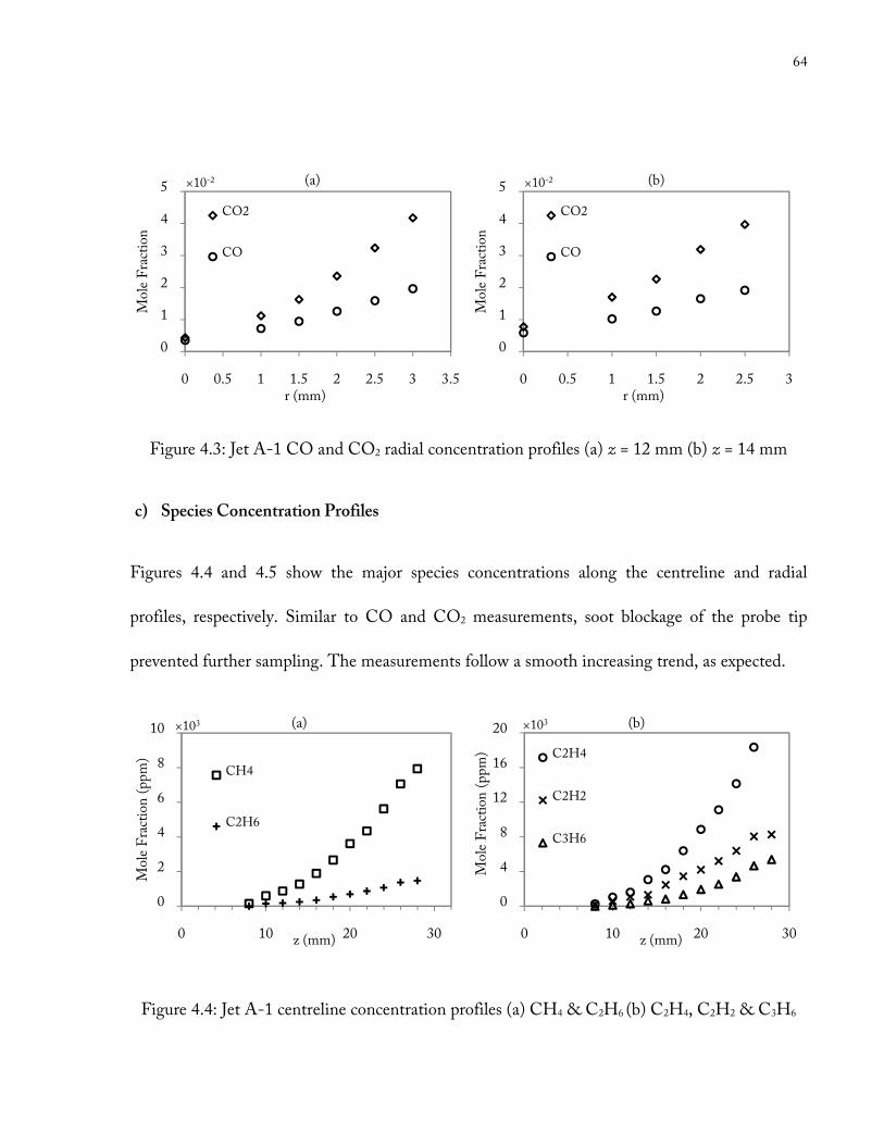
64

Figure 4.3: Jet A-1 CO and CO2 radial concentration profiles (a) z = 12 mm (b) z = 14 mm

c) Species Concentration Profiles

Figures 4.4 and 4.5 show the major species concentrations along the centreline and radial

profiles, respectively. Similar to CO and CO2 measurements, soot blockage of the probe tip

prevented further sampling. The measurements follow a smooth increasing trend, as expected.

Figure 4.4: Jet A-1 centreline concentration profiles (a) CH4 & C2H6 (b) C2H4, C2H2 & C3H6

0

1

2

3

4

5

0 0.5 1 1.5 2 2.5 3 3.5

Mole Fraction

r (mm)

(a)

CO2

CO

×10-2

0

1

2

3

4

5

0 0.5 1 1.5 2 2.5 3

Mole Fraction

r (mm)

(b)

CO2

CO

×10-2

0

2

4

6

8

10

0 10 20 30

Mole Fraction (ppm)

z (mm)

(a)

CH4

C2H6

×103

0

4

8

12

16

20

0 10 20 30

Mole Fraction (ppm)

z (mm)

(b)

C2H4

C2H2

C3H6

×103

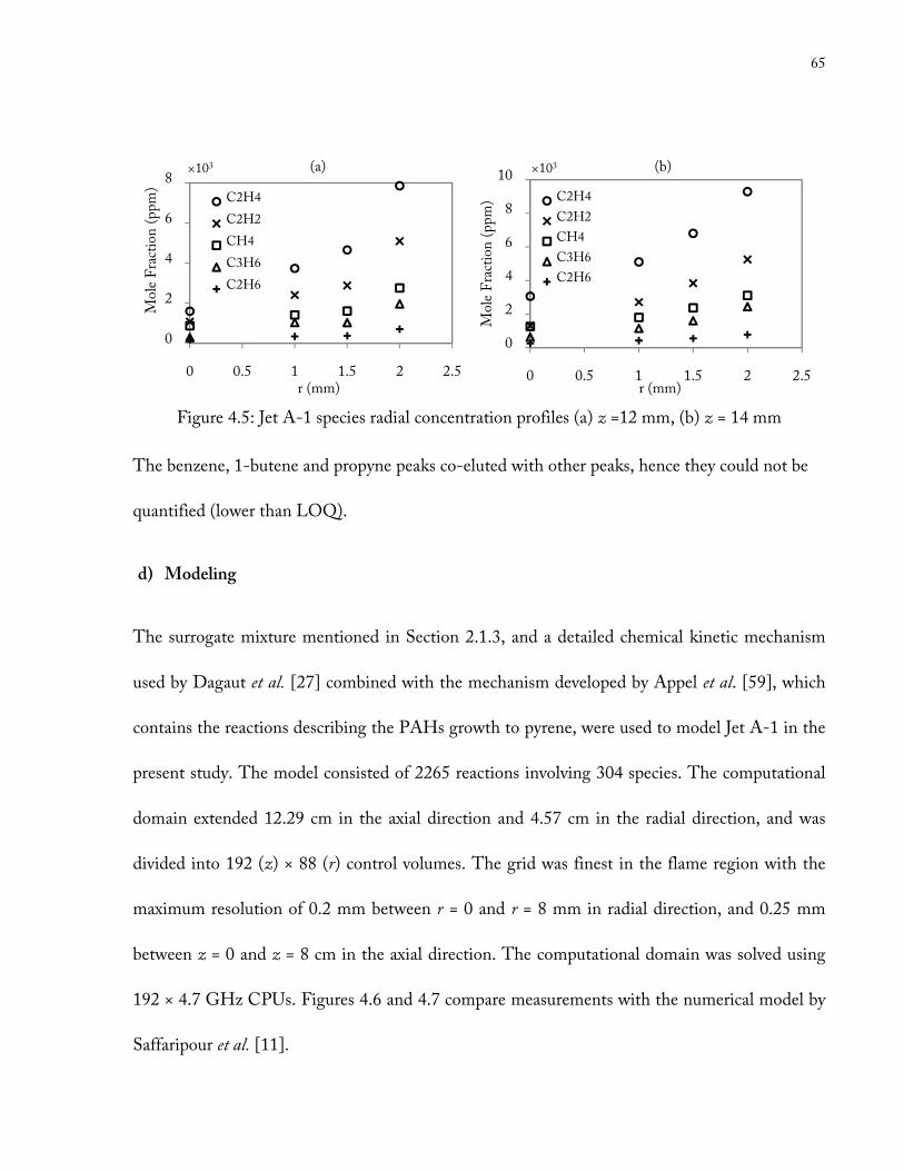
65

Figure 4.5: Jet A-1 species radial concentration profiles (a) z =12 mm, (b) z = 14 mm

The benzene, 1-butene and propyne peaks co-eluted with other peaks, hence they could not be

quantified (lower than LOQ).

d) Modeling

The surrogate mixture mentioned in Section 2.1.3, and a detailed chemical kinetic mechanism

used by Dagaut et al. [27] combined with the mechanism developed by Appel et al. [59], which

contains the reactions describing the PAHs growth to pyrene, were used to model Jet A-1 in the

present study. The model consisted of 2265 reactions involving 304 species. The computational

domain extended 12.29 cm in the axial direction and 4.57 cm in the radial direction, and was

divided into 192 (z) × 88 (r) control volumes. The grid was finest in the flame region with the

maximum resolution of 0.2 mm between r = 0 and r = 8 mm in radial direction, and 0.25 mm

between z = 0 and z = 8 cm in the axial direction. The computational domain was solved using

192 × 4.7 GHz CPUs. Figures 4.6 and 4.7 compare measurements with the numerical model by

Saffaripour et al. [11].

0

2

4

6

8

0 0.5 1 1.5 2 2.5

Mole Fraction(ppm)

r (mm)

(a)

C2H4

C2H2

CH4

C3H6

C2H6

×103

0

2

4

6

8

10

0 0.5 1 1.5 2 2.5

Mole Fraction (ppm)

r (mm)

(b)

C2H4

C2H2

CH4

C3H6

C2H6

×103

66

Figure 4.6: Computational (model) and experimental (exp) comparisons of CO & CO2 mole

fractions for Jet A-1 flame along (a) centreline [11] and (b) radial (z = 12 mm) profiles

Figure 4.7: Computational (model) and experimental (exp) comparison of species centreline

mole fractions for Jet A-1 flame along (a) CH4 & C2H6 (b) C2H4 & C2H2 (c) & C3H6 [11]

0

2

4

6

0 10 20 30

Mole Fraction

z (mm)

(a)

CO2 (exp)

CO2 (model)

CO (exp)

CO (model)

×10-2

0

1

2

3

4

5

0 1 2 3

Mole Fraction

r (mm)

(b)

CO2 (exp)

CO2 (model)

CO (exp)

CO (model)

×10-2

0

2

4

6

8

10

12

0 10 20 30

Mole Fraction (ppm)

z (mm)

(a)CH4 (exp)

CH4 (model)

C2H6 (exp)

C2H6 (model)

× 103

0

10

20

30

40

0 10 20 30

Mole Fraction (ppm)

z (mm)

(b)C2H4 (exp)

C2H4 (model)

C2H2 (exp)

C2H2 (model)

×103

0

2

4

6

8

10

12

0 10 20 30

Mole Fraction (ppm)

z (mm)

(c)

C3H6 (exp)

C3H6 (model)

×103

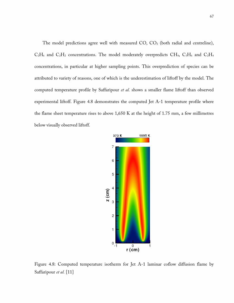
67

The model predictions agree well with measured CO, CO2 (both radial and centreline),

C2H6 and C2H2 concentrations. The model moderately overpredicts CH4, C3H6 and C2H4

concentrations, in particular at higher sampling points. This overprediction of species can be

attributed to variety of reasons, one of which is the underestimation of liftoff by the model. The

computed temperature profile by Saffaripour et al. shows a smaller flame liftoff than observed

experimental liftoff. Figure 4.8 demonstrates the computed Jet A-1 temperature profile where

the flame sheet temperature rises to above 1,650 K at the height of 1.75 mm, a few millimetres

below visually observed liftoff.

Figure 4.8: Computed temperature isotherm for Jet A-1 laminar coflow diffusion flame by

Saffaripour et al. [11]

68

In addition to experimental (systematic and human) errors, three possible sources of errors in

the model may be present: (1) combined Appel and Dagaut jet fuel chemical kinetic

mechanisms, (2) input fuel and oxidizer exit temperature from nozzle, and (3) the fuel surrogate.

Dr. Dworkin, one of the coauthors on the modeling study by Saffaripour et al., suggests that the

error in the predicted liftoff may originate from elimination of a few essential ignition reactions

in mechanism [60]. The largest difference between model and experiments was observed in the

case of ethylene concentration. Ethylene, as one of the most important species in soot formation

(see Section 2.4), could have been miscalculated by the model. It should be noted that soot

concentration computation is one of the weaknesses of the model at the current stage. The liftoff

is also very sensitive to the temperature boundary conditions at the fuel and oxidizer exit [60].

Besides, surrogate fuel used in this model consists of normal paraffinic (69% n-decane) and no

branched paraffinic, while the analysis by ARC (Table 3-1) showed more than 13% of iso-

paraffinics in Jet A-1. The numerical and experimental works done by Sarathy et al. [61]

compared gaseous species from n-octane and 2-methylheptane (branched octane isomer) in

opposed-flow diffusion flames. This study showed that n-octane flame produces approximately

50% more ethylene than 2-methylheptane flame. Hence, it is expected that substituting a few

percentages of n-decane in the surrogate fuel with branched isomers of decane, for instance 2-

methylnonane, may noticeably reduce the predicted ethylene concentrations by the model. Note

that iso-decane was the largest iso-paraffinic compound in Jet A-1 analysis (refer to Table 3-1).

69

Error bars are shown in Figure 4.6 and 4.7. Based on a number of trials and sensitivity

analyses, different errors have been suggested for the comparisons between measured and

computed data. The +1 mm right-sided horizontal error bars show inaccuracy in centring the

probe (location in the z direction). The left-sided horizontal error bars, not only consider the

imprecision of centring the probe, but also includes ~ 2 mm liftoff which is not well represented

in the model predictions. Thus, the left-sided horizontal error bars are -3 mm. Another way to

represent the liftoff is to shift the model 2 mm to the right (positive direction of z axis). In

general, the ±1 mm error bars for each data point are below 15% of total covered sampling

height. For instance at the height of 10 mm, the horizontal error bar is 10% (1 mm/10 mm), and

at the height of 25 mm it is 4% (1 mm/25 mm). The vertical error bars of ±15%, on the other

hand, correspond to the errors involved with calibration, GC analyses and/or any possible leak.

The vertical error bars are determined based on relative standard deviation (RSD) of all four

trials. All things considered, the agreement is excellent between numerical and experimental

results.

In general, for all other fuels a conservative value of ±15% uncertainties were considered in

concentration calculation (vertical bars) and ±1 mm for errors associated with centring the probe

(horizontal bars). To avoid redundancy, the error bars are not shown on the graphs for other

fuels.

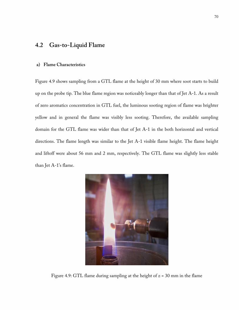
70

4.2 Gas-to-Liquid Flame

a) Flame Characteristics

Figure 4.9 shows sampling from a GTL flame at the height of 30 mm where soot starts to build

up on the probe tip. The blue flame region was noticeably longer than that of Jet A-1. As a result

of zero aromatics concentration in GTL fuel, the luminous sooting region of flame was brighter

yellow and in general the flame was visibly less sooting. Therefore, the available sampling

domain for the GTL flame was wider than that of Jet A-1 in the both horizontal and vertical

directions. The flame length was similar to the Jet A-1 visible flame height. The flame height

and liftoff were about 56 mm and 2 mm, respectively. The GTL flame was slightly less stable

than Jet A-1’s flame.

Figure 4.9: GTL flame during sampling at the height of z = 30 mm in the flame

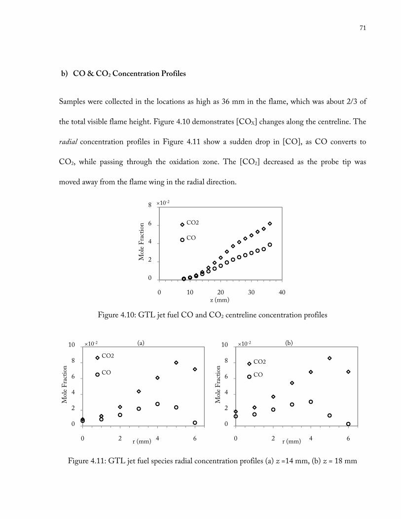
71

b) CO & CO2 Concentration Profiles

Samples were collected in the locations as high as 36 mm in the flame, which was about 2/3 of

the total visible flame height. Figure 4.10 demonstrates [COX] changes along the centreline. The

radial concentration profiles in Figure 4.11 show a sudden drop in [CO], as CO converts to

CO2, while passing through the oxidation zone. The [CO2] decreased as the probe tip was

moved away from the flame wing in the radial direction.

Figure 4.10: GTL jet fuel CO and CO2 centreline concentration profiles

Figure 4.11: GTL jet fuel species radial concentration profiles (a) z =14 mm, (b) z = 18 mm

0

2

4

6

8

0 10 20 30 40

Mole Fraction

z (mm)

CO2

CO

×10-2

0

2

4

6

8

10

0 2 4 6

Mole Fraction

r (mm)

(a)

CO2

CO

×10-2

0

2

4

6

8

10

0 2 4 6

Mole Fraction

r (mm)

(b)

CO2

CO

×10-2

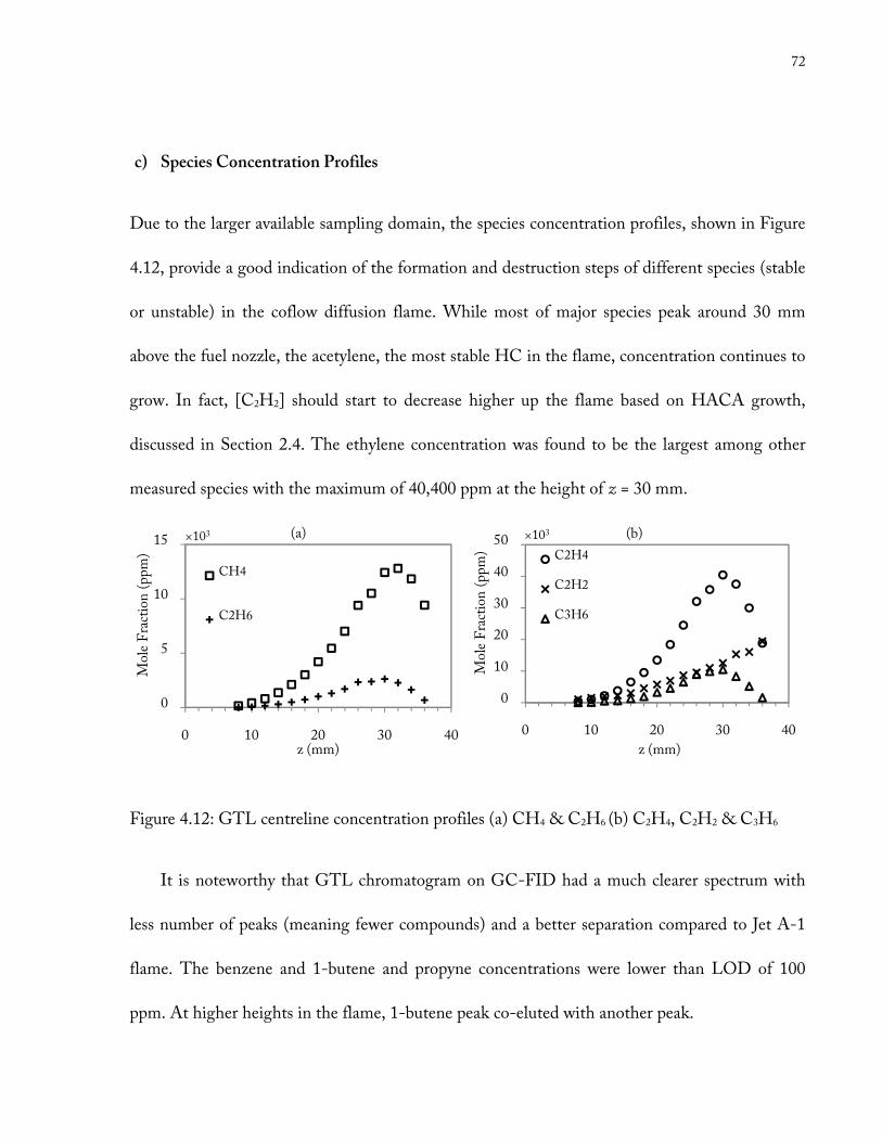
72

c) Species Concentration Profiles

Due to the larger available sampling domain, the species concentration profiles, shown in Figure

4.12, provide a good indication of the formation and destruction steps of different species (stable

or unstable) in the coflow diffusion flame. While most of major species peak around 30 mm

above the fuel nozzle, the acetylene, the most stable HC in the flame, concentration continues to

grow. In fact, [C2H2] should start to decrease higher up the flame based on HACA growth,

discussed in Section 2.4. The ethylene concentration was found to be the largest among other

measured species with the maximum of 40,400 ppm at the height of z = 30 mm.

Figure 4.12: GTL centreline concentration profiles (a) CH4 & C2H6 (b) C2H4, C2H2 & C3H6

It is noteworthy that GTL chromatogram on GC-FID had a much clearer spectrum with

less number of peaks (meaning fewer compounds) and a better separation compared to Jet A-1

flame. The benzene and 1-butene and propyne concentrations were lower than LOD of 100

ppm. At higher heights in the flame, 1-butene peak co-eluted with another peak.

0

5

10

15

0 10 20 30 40

Mole Fraction (ppm)

z (mm)

(a)

CH4

C2H6

×103

0

10

20

30

40

50

0 10 20 30 40

Mole Fraction (ppm)

z (mm)

(b)

C2H4

C2H2

C3H6

×103

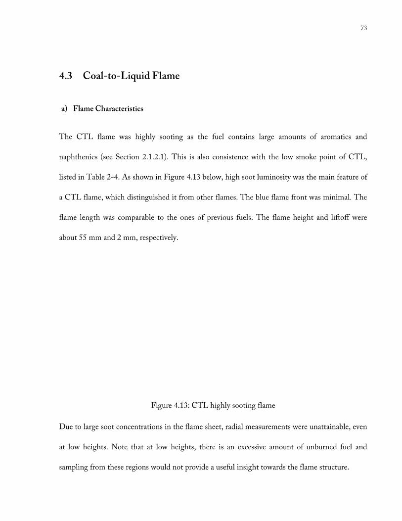
4.3 Coal-to-Liquid

a) Flame Characteristics

The CTL flame was highly sooting

naphthenics (see Section 2.1.2.1

listed in Table 2-4. As shown in

a CTL flame, which distinguished

flame length was comparable to the ones of previous fuels.

about 55 mm and 2 mm, respectively.

Due to large soot concentration

at low heights. Note that at low heights

sampling from these regions

Flame

was highly sooting as the fuel contains large amount

2.1.2.1). This is also consistence with the low smoke point

As shown in Figure 4.13 below, high soot luminosity wa

which distinguished it from other flames. The blue flame front was

flame length was comparable to the ones of previous fuels. The flame height and lift

, respectively.

Figure 4.13: CTL highly sooting flame

Due to large soot concentrations in the flame sheet, radial measurements were unattainable, even

at low heights, there is an excessive amount of unburned fuel and

would not provide a useful insight towards the flame

73

large amounts of aromatics and

low smoke point of CTL,

below, high soot luminosity was the main feature of

. The blue flame front was minimal. The

The flame height and liftoff were

in the flame sheet, radial measurements were unattainable, even

excessive amount of unburned fuel and

flame structure.

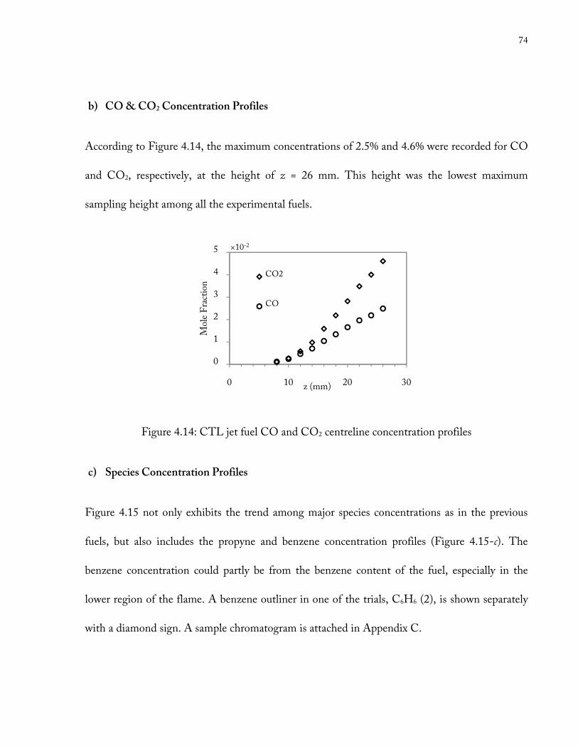
74

b) CO & CO2 Concentration Profiles

According to Figure 4.14, the maximum concentrations of 2.5% and 4.6% were recorded for CO

and CO2, respectively, at the height of z = 26 mm. This height was the lowest maximum

sampling height among all the experimental fuels.

Figure 4.14: CTL jet fuel CO and CO2 centreline concentration profiles

c) Species Concentration Profiles

Figure 4.15 not only exhibits the trend among major species concentrations as in the previous

fuels, but also includes the propyne and benzene concentration profiles (Figure 4.15-c). The

benzene concentration could partly be from the benzene content of the fuel, especially in the

lower region of the flame. A benzene outliner in one of the trials, C6H6 (2), is shown separately

with a diamond sign. A sample chromatogram is attached in Appendix C.

0

1

2

3

4

5

0 10 20 30

Mole Fraction

z (mm)

CO2

CO

×10-2

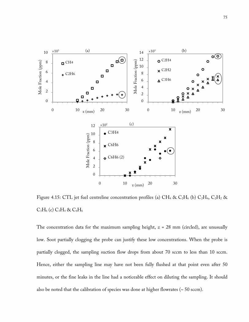
75

Figure 4.15: CTL jet fuel centreline concentration profiles (a) CH4 & C2H6 (b) C2H4, C2H2 &

C3H6 (c) C3H4 & C6H6

The concentration data for the maximum sampling height, z = 28 mm (circled), are unusually

low. Soot partially clogging the probe can justify these low concentrations. When the probe is

partially clogged, the sampling suction flow drops from about 70 sccm to less than 10 sccm.

Hence, either the sampling line may have not been fully flushed at that point even after 50

minutes, or the fine leaks in the line had a noticeable effect on diluting the sampling. It should

also be noted that the calibration of species was done at higher flowrates (~ 50 sccm).

0

2

4

6

8

10

0 10 20 30

Mole Fraction (ppm)

z (mm)

(a)

CH4

C2H6

×103

0

2

4

6

8

10

12

14

0 10 20 30

Mole Fraction (ppm)

z (mm)

(b)

C2H4

C2H2

C3H6

×103

0

2

4

6

8

10

12

0 10 20 30

Mole Fraction (ppm)

z (mm)

(c)

C3H4

C6H6

C6H6 (2)

×102

76

4.4 Gas-to-Liquid Blend with Hexanol Flame

Similar to the GTL fuel, this blend has no aromatics and therefore, a low sooting flame was

expected. The Hex20-GTL fuel has a strong fruity (apple) odour, which is attributed to the

presence of hexanol. The 20 vol.% of hexanol in the fuel is large enough to potentially increase

the concentration of some important oxygenated compounds, such as acetaldehyde and/or

formaldehyde, in its flame. Therefore, the GC-FID was also calibrated for these two species

using the permeation tubes as discussed in Section 3.6.1.3. These compounds were expected to

appear on the rear column of GC-FID, after mixing with hydrogen, passing through the

methanizer and converting to ethane and methane, respectively. In the current study, CH2O and

C2H4O concentrations, however, were below LOQ and their peaks did not secure a certain RT.

Hence, no results are reported on these compounds in this study.

a) Flame Characteristics

The Hex20-GTL flame physical descriptions (e.g. flame height of about 55 mm ± 5 mm,

stability, soot luminosity, etc.) were identical to those of GTL flame. The flame liftoff was 1.8

mm ± 0.2 mm, similar to previous flames.

b) CO & CO2 Concentration Profiles

Figure 4.16 shows [CO] and [CO2] increasing along the centreline. The [CO] and [CO2] peak

at 3.8% and 6.2%, respectively, at the height of 36 mm.

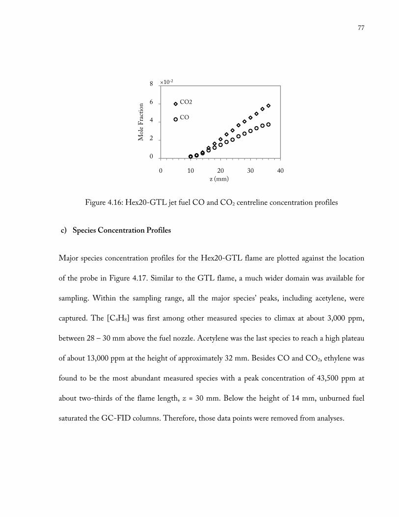
77

Figure 4.16: Hex20-GTL jet fuel CO and CO2 centreline concentration profiles

c) Species Concentration Profiles

Major species concentration profiles for the Hex20-GTL flame are plotted against the location

of the probe in Figure 4.17. Similar to the GTL flame, a much wider domain was available for

sampling. Within the sampling range, all the major species’ peaks, including acetylene, were

captured. The [C4H8] was first among other measured species to climax at about 3,000 ppm,

between 28 – 30 mm above the fuel nozzle. Acetylene was the last species to reach a high plateau

of about 13,000 ppm at the height of approximately 32 mm. Besides CO and CO2, ethylene was

found to be the most abundant measured species with a peak concentration of 43,500 ppm at

about two-thirds of the flame length, z = 30 mm. Below the height of 14 mm, unburned fuel

saturated the GC-FID columns. Therefore, those data points were removed from analyses.

0

2

4

6

8

0 10 20 30 40

Mole Fraction

z (mm)

CO2

CO

×10-2

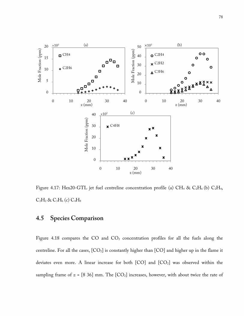
78

Figure 4.17: Hex20-GTL jet fuel centreline concentration profile (a) CH4 & C2H6 (b) C2H4,

C2H2 & C3H6 (c) C4H8

4.5 Species Comparison

Figure 4.18 compares the CO and CO2 concentration profiles for all the fuels along the

centreline. For all the cases, [CO2] is constantly higher than [CO] and higher up in the flame it

deviates even more. A linear increase for both [CO] and [CO2] was observed within the

sampling frame of z = [8 36] mm. The [CO2] increases, however, with about twice the rate of

0

5

10

15

20

0 10 20 30 40

Mole Fraction (ppm)

z (mm)

(a)

CH4

C2H6

×103

0

10

20

30

40

50

0 10 20 30 40

Mole Fraction (ppm)

z (mm)

(b)

C2H4

C2H2

C3H6

×103

0

10

20

30

40

0 10 20 30 40

Mole Fraction (ppm)

z (mm)

(c)

C4H8

×102

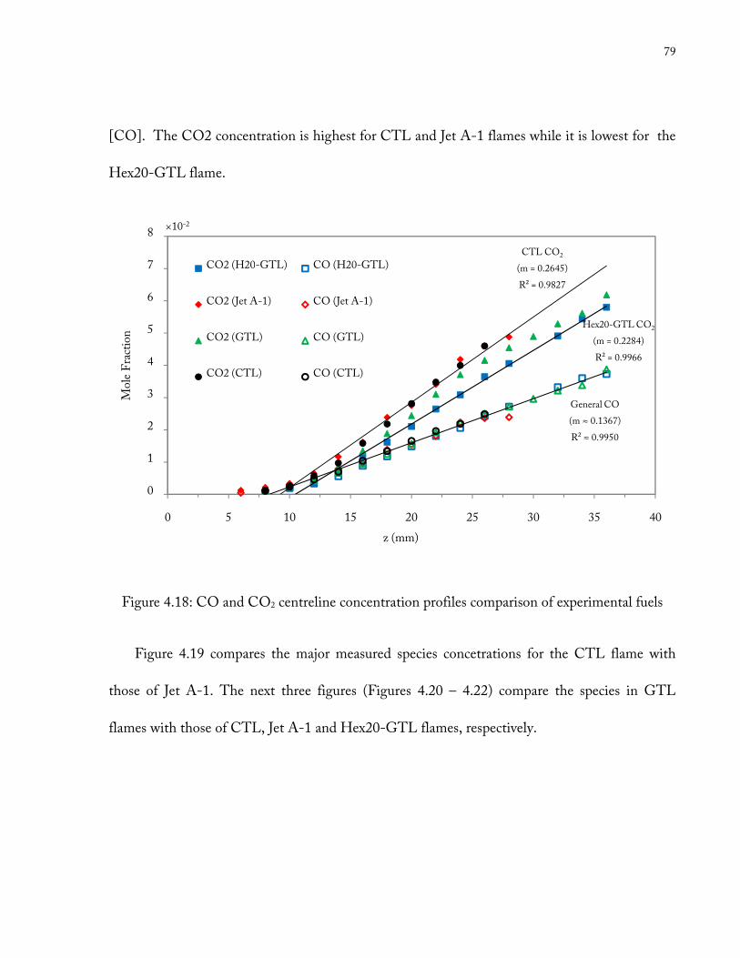
79

[CO]. The CO2 concentration is highest for CTL and Jet A-1 flames while it is lowest for the

Hex20-GTL flame.

Figure 4.18: CO and CO2 centreline concentration profiles comparison of experimental fuels

Figure 4.19 compares the major measured species concetrations for the CTL flame with

those of Jet A-1. The next three figures (Figures 4.20 – 4.22) compare the species in GTL

flames with those of CTL, Jet A-1 and Hex20-GTL flames, respectively.

Hex20-GTL CO2

(m = 0.2284)

R² = 0.9966

General CO

(m ≈ 0.1367)

R² ≈ 0.9950

CTL CO2

(m = 0.2645)

R² = 0.9827

0

1

2

3

4

5

6

7

8

0 5 10 15 20 25 30 35 40

Mole Fraction

z (mm)

CO2 (H20-GTL) CO (H20-GTL)

CO2 (Jet A-1) CO (Jet A-1)

CO2 (GTL) CO (GTL)

CO2 (CTL) CO (CTL)

×10-2

80

Figure 4.19: Species centreline concentration comparison between CTL jet fuel and Jet A-1

A closer look at Figure 4.19 reveals that CTL has slightly higher concentrations of CH4,

C2H6 and C3H6. Note that in the CTL and Jet A-1 flames, which have similar soot luminosity,

the C2H2 and C2H4 concentrations are very similar.

Figure 4.20 compares the GTL and CTL flame species. A group of data points on the GTL

are shown in Figure 4.20 graphs that are within the common sampling domain between both the

GTL and the CTL flames (i.e. 8 ≤ z ≤ 28).

0

2

4

6

8

10

0 10 20 30

Mole Fraction (ppm)

z(mm)

CH4

CTL

Jet A-1

×103

0

0.5

1

1.5

2

0 10 20 30z (mm)

C2H6

CTL

Jet A-1

×103

0

4

8

12

16

20

24

0 10 20 30z(mm)

C2H4

CTL

Jet A-1

×103

0

4

8

12

0 10 20 30

Mole Fraction (ppm)

z (mm)

C2H2

CTL

Jet A-1

×103

0

2

4

6

8

0 10 20 30z (mm)

C3H6

CTL

Jet A-1

×103

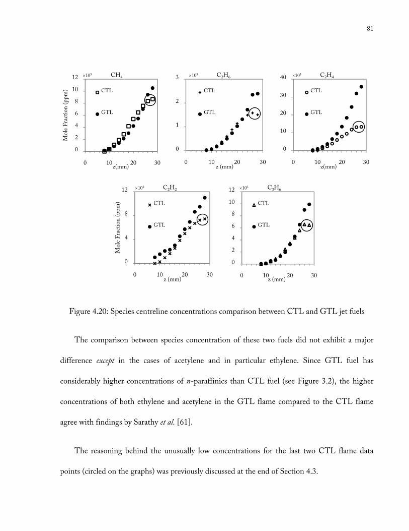
81

Figure 4.20: Species centreline concentrations comparison between CTL and GTL jet fuels

The comparison between species concentration of these two fuels did not exhibit a major

difference except in the cases of acetylene and in particular ethylene. Since GTL fuel has

considerably higher concentrations of n-paraffinics than CTL fuel (see Figure 3.2), the higher

concentrations of both ethylene and acetylene in the GTL flame compared to the CTL flame

agree with findings by Sarathy et al. [61].

The reasoning behind the unusually low concentrations for the last two CTL flame data

points (circled on the graphs) was previously discussed at the end of Section 4.3.

0

2

4

6

8

10

12

0 10 20 30

Mole Fraction (ppm)

z(mm)

CH4

CTL

GTL

×103

0

1

2

3

0 10 20 30z (mm)

C2H6

CTL

GTL

×103

0

10

20

30

40

0 10 20 30z(mm)

C2H4

CTL

GTL

×103

0

4

8

12

0 10 20 30

Mole Fraction (ppm)

z (mm)

C2H2

CTL

GTL

×103

0

2

4

6

8

10

12

0 10 20 30z (mm)

C3H6

CTL

GTL

×103

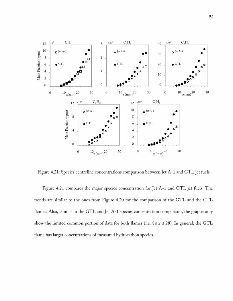
82

Figure 4.21: Species centreline concentrations comparison between Jet A-1 and GTL jet fuels

Figure 4.21 compares the major species concentration for Jet A-1 and GTL jet fuels. The

trends are similar to the ones from Figure 4.20 for the comparison of the GTL and the CTL

flames. Also, similar to the GTL and Jet A-1 species concentration comparison, the graphs only

show the limited common portion of data for both flames (i.e. 8≤ z ≤ 28). In general, the GTL

flame has larger concentrations of measured hydrocarbon species.

0

2

4

6

8

10

12

0 10 20 30

Mole Fraction (ppm)

z(mm)

CH4

Jet A-1

GTL

×103

0

1

2

3

0 10 20 30z (mm)

C2H6

Jet A-1

GTL

×103

0

10

20

30

40

0 10 20 30z(mm)

C2H4

Jet A-1

GTL

×103

0

4

8

12

0 10 20 30

Mole Fraction (ppm)

z (mm)

C2H2

Jet A-1

GTL

×103

0

2

4

6

8

10

12

0 10 20 30z (mm)

C3H6

Jet A-1

GTL

×103

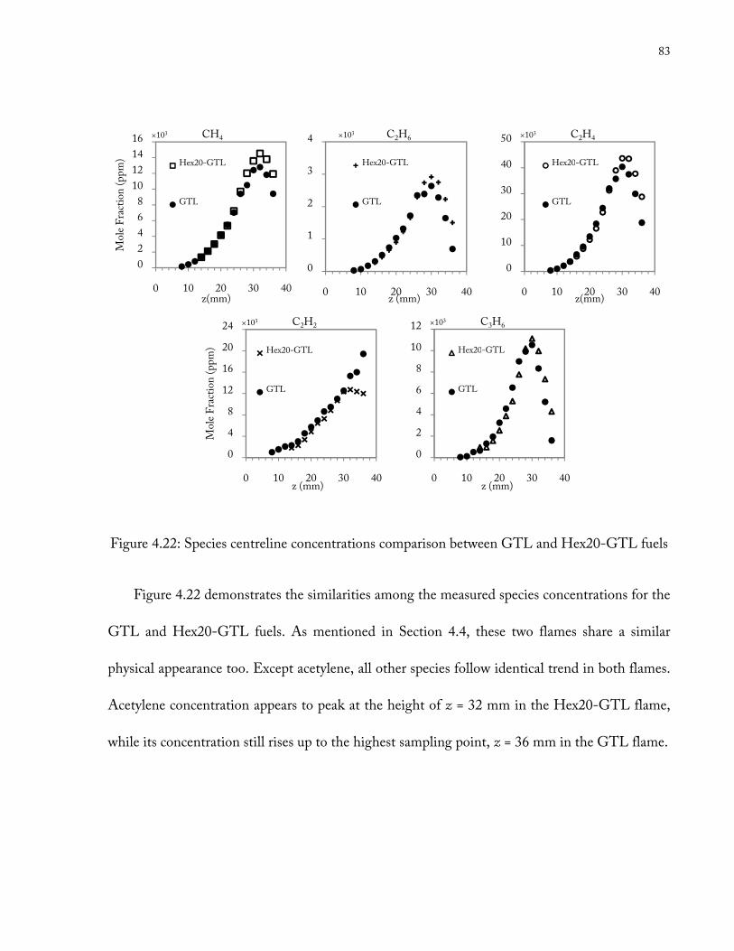
83

Figure 4.22: Species centreline concentrations comparison between GTL and Hex20-GTL fuels

Figure 4.22 demonstrates the similarities among the measured species concentrations for the

GTL and Hex20-GTL fuels. As mentioned in Section 4.4, these two flames share a similar

physical appearance too. Except acetylene, all other species follow identical trend in both flames.

Acetylene concentration appears to peak at the height of z = 32 mm in the Hex20-GTL flame,

while its concentration still rises up to the highest sampling point, z = 36 mm in the GTL flame.

0

2

4

6

8

10

12

14

16

0 10 20 30 40

Mole Fraction (ppm)

z(mm)

CH4

Hex20-GTL

GTL

×103

0

1

2

3

4

0 10 20 30 40z (mm)

C2H6

Hex20-GTL

GTL

×103

0

10

20

30

40

50

0 10 20 30 40z(mm)

C2H4

Hex20-GTL

GTL

×103

0

4

8

12

16

20

24

0 10 20 30 40

Mole Fraction (ppm)

z (mm)

C2H2

Hex20-GTL

GTL

×103

0

2

4

6

8

10

12

0 10 20 30 40z (mm)

C3H6

Hex20-GTL

GTL

×103

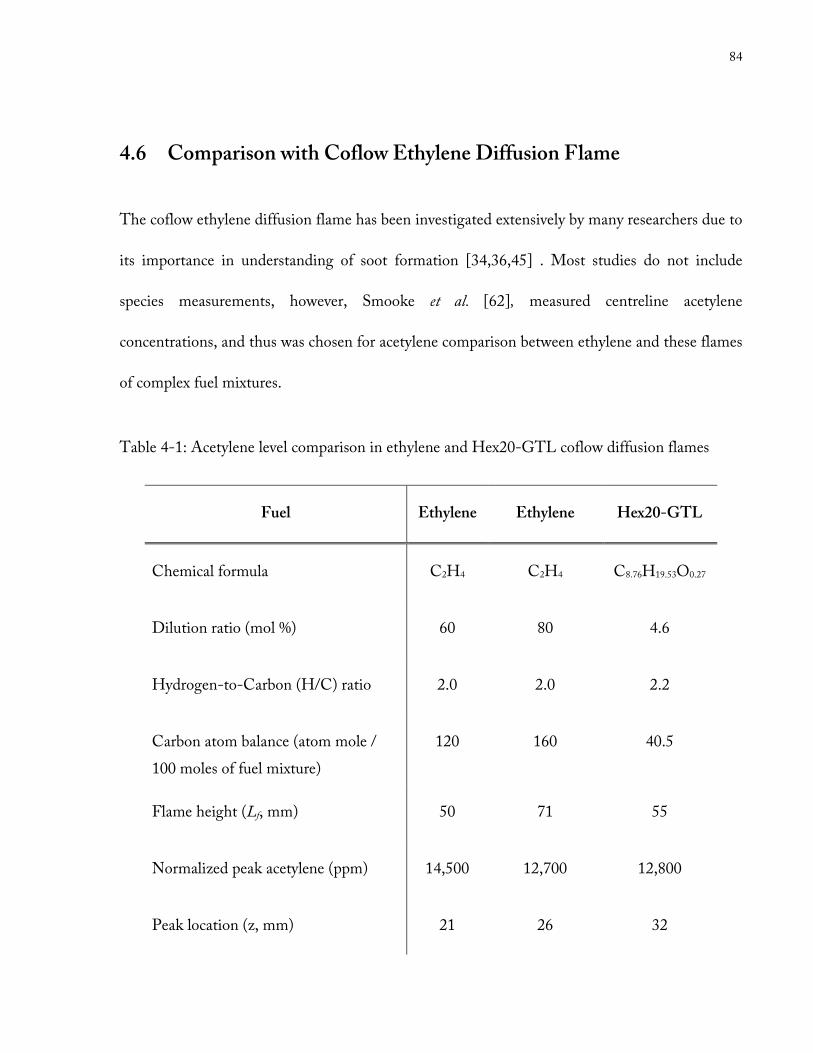
84

4.6 Comparison with Coflow Ethylene Diffusion Flame

The coflow ethylene diffusion flame has been investigated extensively by many researchers due to

its importance in understanding of soot formation [34,36,45] . Most studies do not include

species measurements, however, Smooke et al. [62], measured centreline acetylene

concentrations, and thus was chosen for acetylene comparison between ethylene and these flames

of complex fuel mixtures.

Table 4-1: Acetylene level comparison in ethylene and Hex20-GTL coflow diffusion flames

Fuel Ethylene Ethylene Hex20-GTL

Chemical formula C2H4 C2H4 C8.76H19.53O0.27

Dilution ratio (mol %) 60 80 4.6

Hydrogen-to-Carbon (H/C) ratio 2.0 2.0 2.2

Carbon atom balance (atom mole /

100 moles of fuel mixture)

120 160 40.5

Flame height (Lf, mm) 50 71 55

Normalized peak acetylene (ppm) 14,500 12,700 12,800

Peak location (z, mm) 21 26 32

85

The Hex20-GTL flame data set was chosen because it includes the acetylene peak. Hence,

the maximum concentration of the C2H2 in Hex20-GTL flame was compared with the

normalized peak concentration of C2H2 in ethylene coflow flames. The normalized acetylene

peak was calculated based on maximum acetylene concentration in the mentioned study by

Smooke et al. multiplied by the ratio of dilution. The sample calculations is shown in Appendix

E. In the study by Smooke et al., ethylene was diluted with nitrogen at different dilution ratios.

As it can be seen from Table 4-1, the normalized peak for acetylene is relatively in a same range

as of acetylene concentration in Hex20-GTL flame. Note that the flames for this experiment are

lifted while the flames in mentioned study by Smooke et al. are not.

86

Chapter 5

5. Conclusions & Recommendations

This study investigated gaseous species concentration profiles in sooting laminar jet fuel coflow

diffusion flames. The developed method for vaporizing the jet fuel was proven to be robust, and

the flames produced were stable. Extra precaution was taken into consideration for centring the

burner and taking measurements in order to produce repeatable measurements. The results were

reproducible with a relative standard deviation (RSD) of 10%. The conservative ±15%

uncertainty was considered for the concentration measurements in this study. This value was

obtained based on rigorous sensitivity analyses and multiple trials.

5.1 Conclusions

The performance of the Controlled Evaporative Mixer unit in vapourizing jet fuels was

extremely satisfactory. The residence time for the vapourizer, the lag time between commending

a change on the control box and observing the result in the flame, was less than 10 seconds.

The new sampling setup has two main advantages. On one hand, the sampling flowrate was

large enough that steady state was often reached within 5 – 10 minutes, depending on the

location of the probe. The suction flowrate, on the other hand, was low enough to leave the

flame intact.

87

The visible flame heights for all the flames were observed about 55 mm. The liftoff was kept

below 2 mm at the maximum value of 1.8 mm ± 0.2 mm.

This study provides valuable set of experimental data on coflow flame characterization of Jet

A-1 and other alternative synthetic jet fuels used in this study. These data can be used to validate

the model similar to the ones shown for Jet A-1.

While CO2 centreline concentration varied from one fuel to another, CO concentrations

were almost identical for all the fuels. The Jet A-1 and CTL flames had the highest CO2

concentrations, while the lowest concentrations of CO2 were observed in the Hex20-GTL flame.

Concentration profiles of species, except ethylene, were relatively similar among all the fuels.

The concentrations of the most abundant species in the flame from the highest to the lowest

were; CO2, CO, C2H4, CH4, C2H2, C3H6 and C2H6. Results from both GTL and Hex20-GTL

flames indicate that the concentrations of measured species reached their maximums at the

heights between 28 mm to 32 mm. These two flames produced very close concentrations of

major species. C6H6 and C3H4 were measured in CTL flames, whereas 1-butene was quantified

only in Hex20-GTL flame. The higher concentration of C2H4 and C2H2 in GTL flames

compared to CTL flames can be attributed to the higher i-paraffinic content of GTL fuel.

The model by Saffaripour et al. [11] well reproduced the experimentally measured CO, CO2,

C2H6 and C2H2 concentrations in the Jet A-1 flame. Although the CH4 and C3H6 measured

concentrations were slightly overpredicted, they were within experimental uncertainties. The

88

model, however, moderately overpredicted C2H4 concentrations, in particular around the mid

height of the flame. It is concluded that this overprediction was partly due to underestimation of

liftoff by the model and/or lack of i-paraffinic compounds in the surrogate fuel. The comparison

between ethylene and experimental fuels in this study (1) shows that the measurements were

reasonable, (2) the original motivation behind studying the ethylene flames is confirmed.

5.2 In-Progress Work

Temperature measurement by rapid insertion method is under development. This method

employs a 75 µm diameter R-type thermocouple (Pt-Pt/13%Rh). The raw measurements must

be then corrected for radiation heat losses from the thermocouple wires and soot. The soot

volume fraction is also being measured and studied for all the fuels.

A thermal desorption method to measure heavy PAH (e.g. naphthalene, phenanthrene,

pyrene, etc.) concentrations is under investigation. The result of this work will be a valuable

complementary study to the current research. Also, our Combustion Research Group is currently

working on the modeling of GTL, CTL and Hex20-GTL flames.

5.3 Future Works

The study of GTL and naphthenics blend, the fourth alternative jet fuel provided by ALFA-

BIRD, would be very beneficial. This blend is a promising fuel for substituting conventional jet

89

fuel, as both GTL and naphthenic compounds are currently produced in large commercial scale.

Naphthenic HCs provide the missing saturated cyclic structure in SPK fuel.

The Hex20-GTL fuel requires further investigation, in particular, in case of oxygenated

species studies. The GC-FID should be recalibrated for acetaldehyde, formaldehyde and

additionally calibrated for butaldehyde (or any higher aldehydes) and esters.

5.3.1 Recommendations

• Since a more detailed composition of Jet A-1 is in hand for this experiment, a surrogate

fuel can be modified accordingly. For instance, iso-paraffinic group, which composed

more than 13% of Jet A-1, is suggested to be represented by branched alkanes in the new

surrogate fuel. It is also suggested to run experiments on the current surrogate fuel and

compare the results with both experimental and numerical study of Jet A-1.

• The jet fuel model well predicts most of the measurements. However, the model slightly

overpredicts some species concentrations, in particular, for ethylene. It is recommended

that the soot and chemical kinetics model be further refined for a better agreement

between model and experiment for poorly predicted species. Combustion Research

Group is actively working on improving the soot model.

• The temperature and the velocity of the fuel exit should be checked more precisely. This

would possibly improve liftoff prediction by model.

90

• Another GC-FID can be dedicated for detecting larger HC’s than C4-isomers and

expand the temperature ramp on the current GC-FID for better separation of lower

molecular weight species. Use of micro-GC for detection of single species, such as

acetaldehyde, is advised. Hydrogen can be identified by using another TCD running on

argon carrier gas.

• It is strongly recommended to reinvestigate the presence of CH2O and C2H4O in

Hex20-GTL flame. The oven temperature profile on GC-FID needs to be modified for

better separation method. The retention times for CH2O and C2H4O on rear column are

10 and 11.3 min, respectively, using the current method which coincides with many other

C4 and larger isomers’ peaks. By changing the method, achieving a better separation for

these two species and other oxygenated species on the rear column is foreseeable.

• As far as modeling, use GTL for comparison: (1) easier to model the soot because of its

lower concentrations, and (2) more data points in hand to validate model.

• The laser beam used for centring the burner can be more focused, thus, providing a

higher precision in centring.

91

Bibliography

[1] Anonymous. (2010, April) Air Transport Action Group (ATAG). [Online].

http://www.atag.org

[2] L. Starck, N. Jeuland, and X. Montagne. (2008, January) institut francais du petrole (IFP).

[Online]. www.ifp.com

[3] B. Saynor, A. Bauen, and M. Leach. (2003, August) Imperial College Centre for Energy

Policy and Technology. [Online]. www.iccept.ic.ac.uk

[4] Anonymous. (2010) International Air Transport Association. [Online].

http://www.bsptravellink.iata.org/ps/publications/alternative-fuels.htm

[5] Anonymous. (2010, June) International Air Transport Association. [Online].

http://www.iata.org/pressroom/facts_figures/fact_sheets/Pages/alt_fuels.aspx

[6] P. Dagaut and M. Cathonnet, "The ignition, oxidation, and combustion of kerosene: a

review of experimental and kinetic modeling," Progress in Energy and Combustion Science,

vol. 32, pp. 48-92, 2006.

[7] J. B. Moss and I. M. Aksit, "Modelling soot formation in a laminar diffusion flame

92

burning a surrogate kerosene fuel," in Proceedings of the Combustion Institute, 2007, pp.

3139-3146.

[8] S. Humer et al., "Experimental and kinetic modeling study of combustion of JP-8, its

surrogates amd referemce components in laminar nonpremixed flows," in Proceedings of the

Combustion Institue, 2007, pp. 393-400.

[9] J. A. Cooke et al., "Computational and experimental study of JP-8, a surrogate, and its

componenets in counterflow diffusion flames," in Proceedings of the Combustion Institue,

2005, pp. 439-446.

[10] H. Bufferand, L. Tosatto, B. La Mantia, M. D. Smooke, and A. Gomez, "Experimental

and computational study of methane counterflow diffusion flames perturbed by trace

amounts of either jet fuel or a 6-component surrogate under non-sooting conditions,"

Combustion and Flame, vol. 156, pp. 1594-1603, March 2009.

[11] M. Saffaripour et al., "A numerical and experimental study of a laminar sooting coflow Jet-

A1 diffusion flame," in Proceedings of the Combustion Institute, Beijing, 2010.

[12] S. M. DeCorso, R. A. Symonds, and G. Vermes, "Crude oil firing in the utility gas

turbine," ASME, New York, November 1971.

[13] W. G. Dukek, "Aviation and other gas turbine fuels," ECT, vol. 3, no. 3, pp. 328-351,

93

December 2000.

[14] G. Hemighaus et al. (2006) Aviation Fuels Technical Review. Chevron Global Aviation.

[15] P. A. Muzzell, B. J McKay, E. R. Sattler, L. L. Stavinoha, and R. A. Alvarez, "The effect

of switch-loading fuels on fuel-wetted elastomers," SAE International, vol. 116, no. 5, pp.

1453-1469, April 2007.

[16] J. Bauldreay, "ALFA-BIRD WP1.2 fuels characterisation," Shell UK, Toulouse, Progress

report 2010.

[17] R. N. Hazlett, Thermal oxidation stability of aviation turbine fuels, R. N. Hazlett, Ed.

Philadelphia, USA: ASTM International, 1991.

[18] Anonymous. (2010, June) Air Transport Association. [Online].

http://www.airlines.org/Energy/FuelCost/Pages_Admin/FuelCost.aspx

[19] Anonymous. (2009, September) Shell Ltd. [Online].

http://www.shell.com/home/content/media/news_and_library/press_releases/2009/gtl_jet

_fuel_approved_29092009.html

[20] L. Starck, N. Jeuland, and S. Mendez, "WP 1.2: Fuels chemistry, fuels characterization,"

Institut Francais du Petrole (IFP), Toulouse, Progress report 2010.

94

[21] P. Roets. (2009, Feburary) Sasol synthetic fuels: Cola-to-Liquids. ICAO Workshop -

Aviation and alternative fuels.

[22] Anonymous. (2010, Feburary) Sasol. [Online]. http://www.sasol.com

[23] S. Shulga, Y. Blum, and A. Tkachenko, "Biotechnology and effective strains – producers

of biobutanol," New Biotechnology, vol. 25, no. 1, p. 256, September 2009.

[24] G. Hess, "BP and DuPont to make biobutanol," Chemical & Engineering News, vol. 84,

pp. 9-10, August 2006.

[25] D. W. Verser, "Indirect production of butanol and hexanol," PCT/US2009/033561,

August 13, 2009.

[26] L. Starck, N. Jeuland, G. Zalamansky, and A. Westenberger, "Overview of possible

alternative fuels and selection of alternative fuels," EU-VRi (ALFA-BIRD), ACP7-GA-

2008-213266, 2009.

[27] P. Dagaut and S. Gail, "Chemical kinetic study of the effect of biofuel additive on Jet A-1

combustion," Journal of Physics & Chemistry, vol. 111, pp. 3992-4000, 2007.

[28] P. Dagaut, ALFA-BIRD alternative jet fuel surrogates, 2010, E-mail communication.

95

[29] S. Hu et al., "Aircraft emission impact in a neighborhood adjacent to a general aviation

airport in Southern California," Environmental Science & Technology, vol. 43, no. 21, p.

8039–8045, October 2009.

[30] J. H. Ware et al., "Effects of ambient sulfur oxides and suspended particles on respiratory

health of preadolescent children," The American review of respiratory disease, vol. 5, pp. 834-

842, May 1986.

[31] D. L. Mauzerall, B. Sultan, N. Kim, and D. F. Bradford, "NOx emissions from large point

sources: variability in ozone production, resulting health damages and economic costs,"

Atmospheric Environment, vol. 39, no. 16, pp. 2851-2866, May 2005.

[32] R. Sharifi, S. V. Pisupati, and A. W. Scaroni, "Combustion science and technology.," in

Kirk-Othmer Encyclopedia of Chemical Technology. New York, USA: John Wiley & Sons,

1993, pp. 435-479.

[33] R. J. Santoro and H. G. Semerjian, "Soot formation in diffusion flames: Flow rate, fuel

species and temperature effects," Symposium (International) on Combustion, vol. 20, no. 1,

pp. 997-1006 , 1985.

[34] R. J. Santoro, H. G. Semerjian, and R. A. Dobbins, "Soot particle measurements in

diffusion flames," Combustion and Flame, vol. 51, pp. 203-218, December 1983.

96

[35] R. J. Santoro, T. T. Yeh, J. J. Horvath, and H. G. Semerijian, "The transport and growth

of soot particles in laminar diffusion flames," Combustion Science & Technology, vol. 53, no.

2, pp. 89-115, 1987.

[36] M. D. Smooke, M. B. Long, B. C. Connelly, M. B. Colket, and R. J. Hall, "Soot

formation in laminar diffusion flames," Combustion and Flame, vol. 143, pp. 613-628,

August 2005.

[37] H. S. Hura and I. Glassman, "Soot formation in diffusion flames of fuel/oxygen mixtures,"

Symposium (International) on Combustion, vol. 22, no. 1, pp. 371-378 , 1989.

[38] N. Peters, Turbulent combustion, 1st ed., G. K. Batchelor, Ed. Cambridge, United

Kingdom: Cambridge University Press, 2000.

[39] S. R. Turns, An introduction to combustion: concepts and applications, 2nd ed. University

Park, PA, USA: McGraw-Hill, 2000.

[40] F. El-Mahallawy and S. El-Din Habik, Fundamentals and technology of combustion, 1st ed.

Egypt: Elsevier Science Ltd., 2002.

[41] A. S. Gordona, S. C. Li, and F. A. Williams, "Visible flame heights of laminar coflow

diffusion flames," Combustion Science & Technology, vol. 141, no. 1, pp. 1-18, 1999.

97

[42] I. Glassman and R. A. Yetter, Combustion, 4th ed. San Diego, CA: Academic Press, 2008.

[43] H. Richter and J. B. Howard, "Formation of polycyclic aromatic hydrocarbons and their

growth to soot - a review of chemical reaction pathways," Progress in Energy and

Combustion Science, vol. 26, pp. 656-608, 2000.

[44] C. K. Law, Combustion Physics. New York: Cambridge University Press, 2006.

[45] Ö. Gülder and D. Snelling, "Influence of nitrogen dilution and flame temperature on soot

formation in diffusion flame," Combustion & Flame, vol. 92, pp. 115-124, 1993.

[46] R. C. Millikan, "Non-equilibrium soot formation in premixed flames," Journal of Physical

Chemistry, vol. 66, no. 5, p. 794–799, May 1962.

[47] W. Gao, R. L. Robinson, and K. A. M. Gasem, "High-pressure solubilities of hydrogen,

nitrogen, and carbon monoxide in dodecane from 344 to 410 K at pressures to 13.2 MPa,"

Journal of Chemical engineering Data, vol. 44, no. 1, pp. 130-132, 1999.

[48] J. Tong, W. Gao, R. L. Robinson, and K. A. M. Gasem, "Solubilities of nitrogen in heavy

normal paraffins from 323 to 423 K at pressures to 18.0 MPa," Journal of Chemical

engineering Data, vol. 44, no. 4, p. 784–787, 1999.

[49] F. A. Williams, Combustion theory: The fundamental theory of chemically reacting flow systems,

98

2nd ed., R. W. Mixter, Ed. Princeton NJ, USA: The Benjamin/Cummings Publishing

Company, Inc, 1985.

[50] S. M. Sarathy, "Chemical kinetic modeling of biofuel combustion," University of Toronto,

PhD Thesis 2009.

[51] S. B. Karra and S. M. Senkan, "Chemical structures of sooting CH3Cl/CH4/O2/Ar and

CH4/O2/Ar flames," Combustion Science & Technology, vol. 54, p. 333, 1987.

[52] M. Kassem, M. Qun, and S. M. Senkan, "Chemical structure of fuel-rich 1,2-

C2H4Cl2/CH4/O2/Ar flames: effects of micro-probe cooling on the sampling of flames

of chlorinated hydrocarbons," Combustion Science & Technology, vol. 67, no. 4, pp. 147-157,

1986.

[53] R. M. Fristrom, "Comments of quenching mechanisms in the microprobe sampling of

flames," Combustion & Flame, vol. 50, pp. 239-242, 1983.

[54] R. M. Fristorm and A. Westenberg, Flame Structure. NewYork: McGraw-Hill, 1965.

[55] S. M. Schoenung and R. K. Hanson, "CO and temperature measurements in a flat flame

by laser absorption spectroscopy and probe techniques," Combustion Science & Technology,

vol. 24, no. 5-6, pp. 227-237, 1981.

99

[56] C. Dybowski and M. A. Kaiser, "Chromatography," in Kirk-Othmer Encyclopedia of

Chemical Technology. New York, USA: John Wiley & Sons, January 2002, vol. 6, pp. 373-

390.

[57] J. Pachlhofer and M. Stevens. (2010, July) Varian Inc. [Online].

http://www.varianinc.com.cn/products/chrom/apps/gc59.pdf

[58] K. Schofield, "The enigmatic mechanism of the flame ionization detector: Its overlooked

implications for fossil fuel combustion modeling," Progress in Energy & Combustion Science,

vol. 34, no. 3, pp. 330-350, June 2008.

[59] J. Appel, H. Bockhorn, and M. Frenklach, "Kinetic modeling of soot formation with

detailed chemistry and physics: laminar premixed flames of C2 hydrocarbons," Combustion

& Flame, vol. 121, no. 1-2, pp. 122-136, April 2000.

[60] Dr. Seth Dworkin, Email correspondings, 2010.

[61] S. M. Sarathy et al., "An experimental and kinetic modeling study of n-octane and 2-

methylheptane in an opposed-flow diffusion flame," To be submitted.

[62] M. D. Smooke et al., "Invistigation of the transition from lightly sooting towards heavily

sooting coflow ethylene diffusion flames," Combustion Theory & Modelling, vol. 8, no. 3,

pp. 593-606, June 2004.

100

Appendices

Appendix A: Jet A-1 composition & thermophysical properties of all jet fuels ...................101

Appendix B: Step-by-Step sample analysis on GC-TCD .................................................... 129

Appendix C: Sample gas chromatograms ............................................................................ 133

Appendix D: Governing equations ...................................................................................... 137

Appendix E: Sample calculations ........................................................................................ 141

Appendix A

Part I:

Jet A-1 Fuel Composition

101

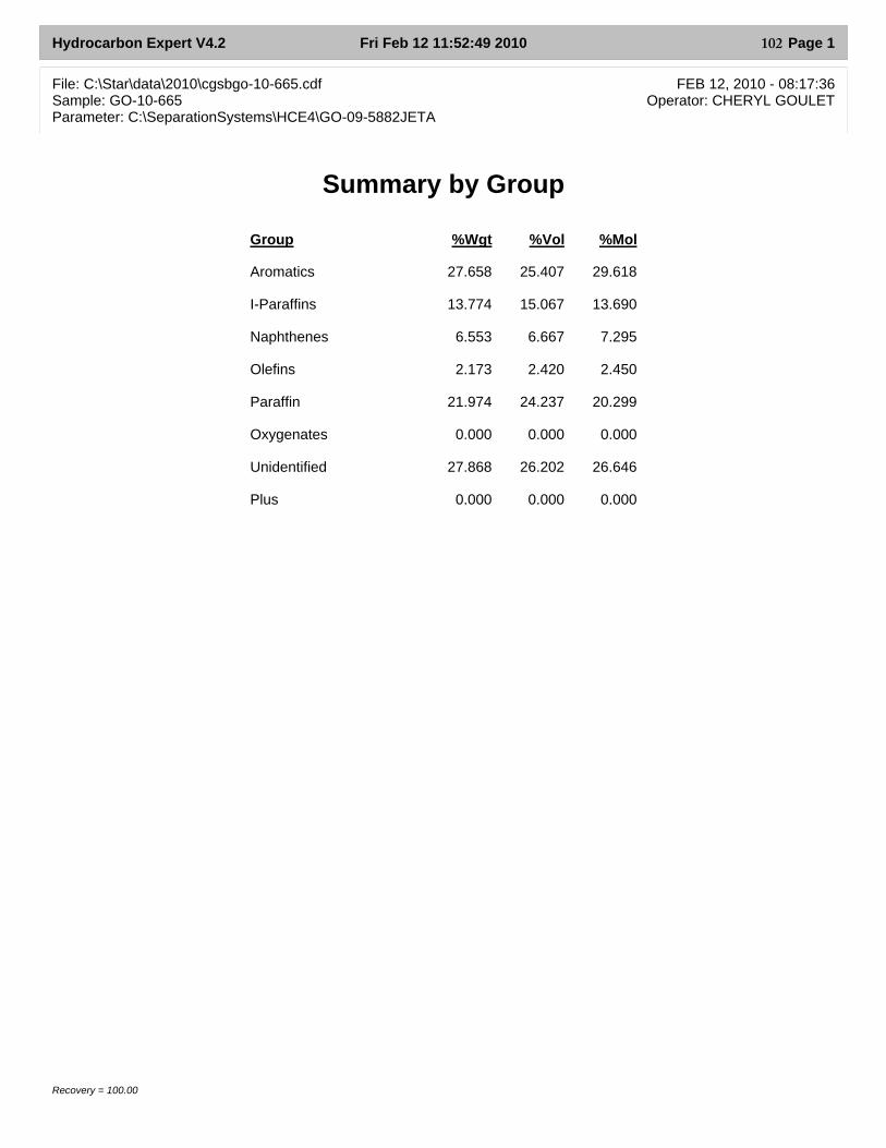
Hydrocarbon Expert V4.2 Fri Feb 12 11:52:49 2010 Page 1

File: C:\Star\data\2010\cgsbgo-10-665.cdf FEB 12, 2010 - 08:17:36Sample: GO-10-665 Operator: CHERYL GOULETParameter: C:\SeparationSystems\HCE4\GO-09-5882JETA

Summary by Group

Recovery = 100.00

Group %Wgt %Vol %Mol

Aromatics 27.658 25.407 29.618

I-Paraffins 13.774 15.067 13.690

Naphthenes 6.553 6.667 7.295

Olefins 2.173 2.420 2.450

Paraffin 21.974 24.237 20.299

Oxygenates 0.000 0.000 0.000

Unidentified 27.868 26.202 26.646

Plus 0.000 0.000 0.000

102

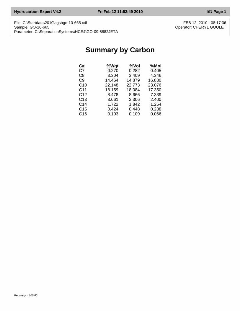
Hydrocarbon Expert V4.2 Fri Feb 12 11:52:49 2010 Page 1

File: C:\Star\data\2010\cgsbgo-10-665.cdf FEB 12, 2010 - 08:17:36Sample: GO-10-665 Operator: CHERYL GOULETParameter: C:\SeparationSystems\HCE4\GO-09-5882JETA

Summary by Carbon

Recovery = 100.00

C# %Wgt %Vol %MolC7 0.270 0.282 0.405C8 3.304 3.409 4.346C9 14.464 14.879 16.830C10 22.148 22.773 23.076C11 18.159 18.084 17.350C12 8.478 8.666 7.339C13 3.061 3.306 2.400C14 1.722 1.842 1.254C15 0.424 0.448 0.288C16 0.103 0.109 0.066

103

Hydrocarbon Expert V4.2 Fri Feb 12 11:52:49 2010 Page 1

File: C:\Star\data\2010\cgsbgo-10-665.cdf FEB 12, 2010 - 08:17:36Sample: GO-10-665 Operator: CHERYL GOULETParameter: C:\SeparationSystems\HCE4\GO-09-5882JETA

Composite by Carbon

Recovery = 100.00

Group C# %Wgt %Vol %MolAromatics C7 0.088 0.083 0.138

C8 1.465 1.376 1.994C9 6.064 5.640 7.301

C10 7.656 7.003 8.297C11 8.873 8.038 8.764C12 3.512 3.267 3.125

I-Paraffins C8 0.238 0.275 0.301C9 2.262 2.549 2.549

C10 5.540 6.146 5.628C11 4.566 4.838 4.222C12 1.167 1.259 0.991

Naphthenes C7 0.139 0.148 0.205C8 0.872 0.916 1.124C9 2.239 2.287 2.563

C10 3.303 3.316 3.404

Olefins C8 0.224 0.256 0.289C9 1.341 1.495 1.536

C10 0.607 0.670 0.626

Paraffin C7 0.043 0.051 0.062C8 0.504 0.586 0.638C9 2.558 2.908 2.882

C10 5.041 5.639 5.121C11 4.720 5.208 4.365C12 3.798 4.140 3.223C13 3.061 3.306 2.400C14 1.722 1.842 1.254C15 0.424 0.448 0.288C16 0.103 0.109 0.066

104

Hydrocarbon Expert V4.2 Fri Feb 12 11:52:49 2010 Page 1

File: C:\Star\data\2010\cgsbgo-10-665.cdf FEB 12, 2010 - 08:17:36Sample: GO-10-665 Operator: CHERYL GOULETParameter: C:\SeparationSystems\HCE4\GO-09-5882JETA

Component List

Recovery = 100.00

Pk# Time Group Component %Wgt %Vol %Mol1 14.671 ? Unidentified 0.002 0.003 0.0042 56.971 P7 200 n-Heptane 0.043 0.051 0.0623 60.378 N7 222 Methylcyclohexane 0.139 0.148 0.2054 67.957 A7 300 Toluene 0.088 0.083 0.1385 71.122 I8 326 2-Methylheptane 0.108 0.126 0.1366 71.375 I8 328 4-Methylheptane 0.034 0.039 0.0437 72.264 N8 335 t-1,4-DiMcycloC6 0.163 0.170 0.2118 72.457 I8 338 3-Ethylhexane 0.096 0.110 0.1229 72.620 O8 340 C8-Diolefin 0.089 0.102 0.115

10 73.525 N8 346 1,1-Dimethylcyclohexane 0.028 0.032 0.037

11 74.350 I9 354 2,2,5-Trimethylhexane 0.029 0.033 0.03312 74.702 N8 360 t-1-E-2-McyC5 0.031 0.033 0.04013 74.922 ? Unidentified 0.048 0.051 0.06214 75.620 O8 370 C8-Olefins 0.135 0.154 0.17415 76.888 N8 390 c-1,4-DiMcycloC6 0.081 0.084 0.10416 77.045 P8 400 n-Octane 0.504 0.586 0.63817 80.123 ? Unidentified 0.015 0.016 0.01618 80.524 N8 432 c-1,2-DiMcycloC6 0.044 0.045 0.05719 80.741 I9 434 2,4-Dimethylheptane 0.075 0.086 0.08520 81.342 N8 442 Propylcyclopentane 0.525 0.552 0.676

21 81.712 N9 450 1,1,3-TriMcycloC6 0.159 0.167 0.18222 82.155 O9 452 C9-Olefins 0.285 0.320 0.32623 82.510 ? Unidentified 0.036 0.041 0.04124 82.643 I9 458 2,5 & 3,5-DMheptane 0.126 0.142 0.14225 82.823 ? Unidentified 0.028 0.032 0.03226 82.947 O9 460 C9-Olefins 0.028 0.031 0.03227 83.128 I9 462 3,3-Dimethylheptane 0.050 0.057 0.05628 83.353 I9 466 C9-Isoparaffin 0.027 0.031 0.03129 83.947 A8 475 Ethylbenzene 0.240 0.226 0.32630 84.133 O9 482 C9-Olefins 0.099 0.111 0.113

31 84.350 I9 485 2,3,4-Trimethylhexane 0.179 0.197 0.20132 84.618 O9 490 C9-Olefins 0.021 0.023 0.02433 85.166 A8 500 m-Xylene 0.598 0.565 0.81534 85.323 A8 502 p-Xylene 0.186 0.176 0.25335 85.495 I9 503 2,3-Dimethylheptane 0.228 0.255 0.25736 85.750 ? Unidentified 0.021 0.023 0.02437 85.941 O9 508 C9-Olefin 0.099 0.111 0.11438 86.148 I9 510 3-Methyl-3-ethylhexane 0.060 0.066 0.06839 86.313 ? Unidentified 0.015 0.017 0.01740 86.555 I9 518 4-MC8+C9-Olefin 0.265 0.301 0.299

41 86.693 I9 520 2-Methyloctane 0.339 0.389 0.38242 87.089 O9 522 C9-Olefin 0.041 0.046 0.04743 87.560 I9 530 3-Methyloctane 0.590 0.664 0.66444 88.173 A8 550 o-Xylene 0.441 0.409 0.60045 88.315 ? Unidentified 0.051 0.057 0.058

105

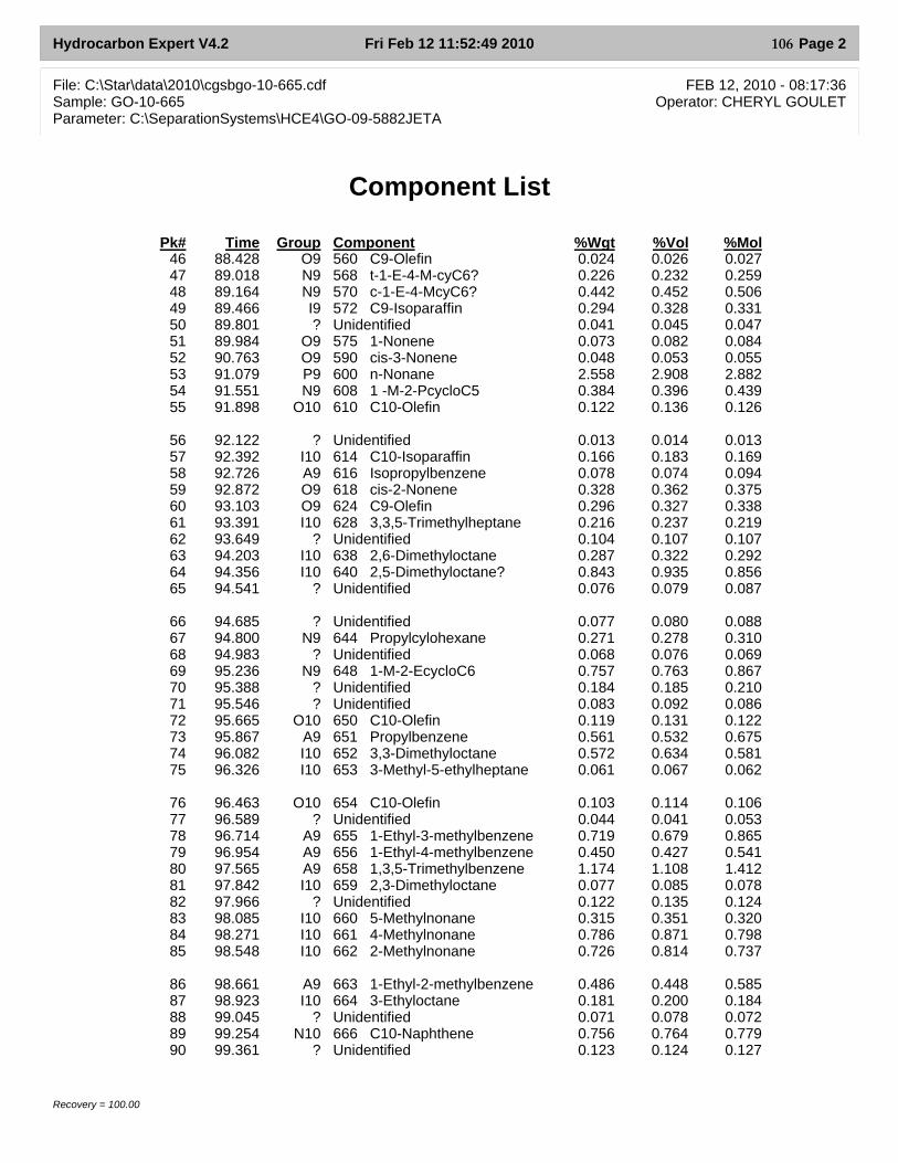
Hydrocarbon Expert V4.2 Fri Feb 12 11:52:49 2010 Page 2

File: C:\Star\data\2010\cgsbgo-10-665.cdf FEB 12, 2010 - 08:17:36Sample: GO-10-665 Operator: CHERYL GOULETParameter: C:\SeparationSystems\HCE4\GO-09-5882JETA

Component List

Recovery = 100.00

Pk# Time Group Component %Wgt %Vol %Mol46 88.428 O9 560 C9-Olefin 0.024 0.026 0.02747 89.018 N9 568 t-1-E-4-M-cyC6? 0.226 0.232 0.25948 89.164 N9 570 c-1-E-4-McyC6? 0.442 0.452 0.50649 89.466 I9 572 C9-Isoparaffin 0.294 0.328 0.33150 89.801 ? Unidentified 0.041 0.045 0.04751 89.984 O9 575 1-Nonene 0.073 0.082 0.08452 90.763 O9 590 cis-3-Nonene 0.048 0.053 0.05553 91.079 P9 600 n-Nonane 2.558 2.908 2.88254 91.551 N9 608 1 -M-2-PcycloC5 0.384 0.396 0.43955 91.898 O10 610 C10-Olefin 0.122 0.136 0.126

56 92.122 ? Unidentified 0.013 0.014 0.01357 92.392 I10 614 C10-Isoparaffin 0.166 0.183 0.16958 92.726 A9 616 Isopropylbenzene 0.078 0.074 0.09459 92.872 O9 618 cis-2-Nonene 0.328 0.362 0.37560 93.103 O9 624 C9-Olefin 0.296 0.327 0.33861 93.391 I10 628 3,3,5-Trimethylheptane 0.216 0.237 0.21962 93.649 ? Unidentified 0.104 0.107 0.10763 94.203 I10 638 2,6-Dimethyloctane 0.287 0.322 0.29264 94.356 I10 640 2,5-Dimethyloctane? 0.843 0.935 0.85665 94.541 ? Unidentified 0.076 0.079 0.087

66 94.685 ? Unidentified 0.077 0.080 0.08867 94.800 N9 644 Propylcylohexane 0.271 0.278 0.31068 94.983 ? Unidentified 0.068 0.076 0.06969 95.236 N9 648 1-M-2-EcycloC6 0.757 0.763 0.86770 95.388 ? Unidentified 0.184 0.185 0.21071 95.546 ? Unidentified 0.083 0.092 0.08672 95.665 O10 650 C10-Olefin 0.119 0.131 0.12273 95.867 A9 651 Propylbenzene 0.561 0.532 0.67574 96.082 I10 652 3,3-Dimethyloctane 0.572 0.634 0.58175 96.326 I10 653 3-Methyl-5-ethylheptane 0.061 0.067 0.062

76 96.463 O10 654 C10-Olefin 0.103 0.114 0.10677 96.589 ? Unidentified 0.044 0.041 0.05378 96.714 A9 655 1-Ethyl-3-methylbenzene 0.719 0.679 0.86579 96.954 A9 656 1-Ethyl-4-methylbenzene 0.450 0.427 0.54180 97.565 A9 658 1,3,5-Trimethylbenzene 1.174 1.108 1.41281 97.842 I10 659 2,3-Dimethyloctane 0.077 0.085 0.07882 97.966 ? Unidentified 0.122 0.135 0.12483 98.085 I10 660 5-Methylnonane 0.315 0.351 0.32084 98.271 I10 661 4-Methylnonane 0.786 0.871 0.79885 98.548 I10 662 2-Methylnonane 0.726 0.814 0.737

86 98.661 A9 663 1-Ethyl-2-methylbenzene 0.486 0.448 0.58587 98.923 I10 664 3-Ethyloctane 0.181 0.200 0.18488 99.045 ? Unidentified 0.071 0.078 0.07289 99.254 N10 666 C10-Naphthene 0.756 0.764 0.77990 99.361 ? Unidentified 0.123 0.124 0.127

106

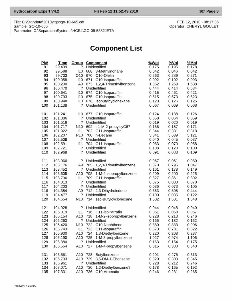
Hydrocarbon Expert V4.2 Fri Feb 12 11:52:49 2010 Page 3

File: C:\Star\data\2010\cgsbgo-10-665.cdf FEB 12, 2010 - 08:17:36Sample: GO-10-665 Operator: CHERYL GOULETParameter: C:\SeparationSystems\HCE4\GO-09-5882JETA

Component List

Recovery = 100.00

Pk# Time Group Component %Wgt %Vol %Mol91 99.439 ? Unidentified 0.175 0.195 0.17892 99.588 I10 668 3-Methylnonane 0.042 0.046 0.04293 99.733 O10 670 C10-Olefin 0.263 0.289 0.27194 100.058 I10 671 C10-Isoparaffin 0.092 0.102 0.09395 100.290 A9 673 1,2,4-Trimethylbenzene 1.362 1.269 1.63896 100.470 ? Unidentified 0.444 0.414 0.53497 100.641 I10 674 C10-Isoparaffin 0.415 0.461 0.42198 100.793 I10 675 C10-Isoparaffin 0.515 0.573 0.52399 100.948 I10 676 Isobutylcyclohexane 0.123 0.126 0.125

100 101.138 ? Unidentified 0.067 0.069 0.068

101 101.241 I10 677 C10-Isoparaffin 0.124 0.138 0.126102 101.386 ? Unidentified 0.058 0.064 0.059103 101.518 ? Unidentified 0.019 0.020 0.019104 101.717 N10 692 t-1-M-2-propylcyC6? 0.166 0.167 0.171105 101.922 I11 702 C11-Isoparaffin 0.344 0.381 0.318106 102.207 P10 700 n-Decane 5.041 5.639 5.121107 102.508 ? Unidentified 0.040 0.045 0.037108 102.591 I11 704 C11-Isoparaffin 0.063 0.070 0.058109 102.721 ? Unidentified 0.108 0.120 0.100110 102.968 ? Unidentified 0.091 0.083 0.109

111 103.066 ? Unidentified 0.067 0.061 0.080112 103.176 A9 705 1,2,3-Trimethylbenzene 0.870 0.795 1.047113 103.452 ? Unidentified 0.161 0.178 0.149114 103.605 A10 708 1-M-4-isopropylbenzene 0.209 0.200 0.225115 103.796 I11 709 C11-Isoparaffin 0.327 0.361 0.302116 104.013 ? Unidentified 0.075 0.083 0.070117 104.203 ? Unidentified 0.086 0.073 0.105118 104.354 A9 712 2,3-Dihydroindene 0.363 0.308 0.444119 104.477 ? Unidentified 0.100 0.085 0.122120 104.654 N10 714 sec-Butylcyclohexane 1.502 1.501 1.548

121 104.928 ? Unidentified 0.044 0.048 0.040122 105.019 I11 716 C11-isoParrafin 0.061 0.068 0.057123 105.154 A10 718 1-M-2-isopropylbenzene 0.228 0.213 0.246124 105.263 ? Unidentified 0.165 0.182 0.152125 105.420 N10 722 C10-Naphthene 0.880 0.883 0.906126 105.743 I11 723 C11-Isoparaffin 0.673 0.731 0.622127 105.930 A10 724 1,3-Diethylbenzene 0.220 0.208 0.237128 106.190 A10 725 1-M-3-propylbenzene 1.027 0.974 1.106129 106.380 ? Unidentified 0.163 0.154 0.175130 106.554 A10 727 1-M-4-propylbenzene 0.315 0.300 0.340

131 106.661 A10 728 Butylbenzene 0.291 0.276 0.313132 106.793 A10 729 3,5-DM-1-Ebenzene 0.320 0.303 0.345133 106.961 ? Unidentified 0.228 0.212 0.246134 107.071 A10 730 1,2-Diethylbenzene? 0.178 0.165 0.192135 107.331 A10 736 C10-Aromatic 0.246 0.231 0.265

107

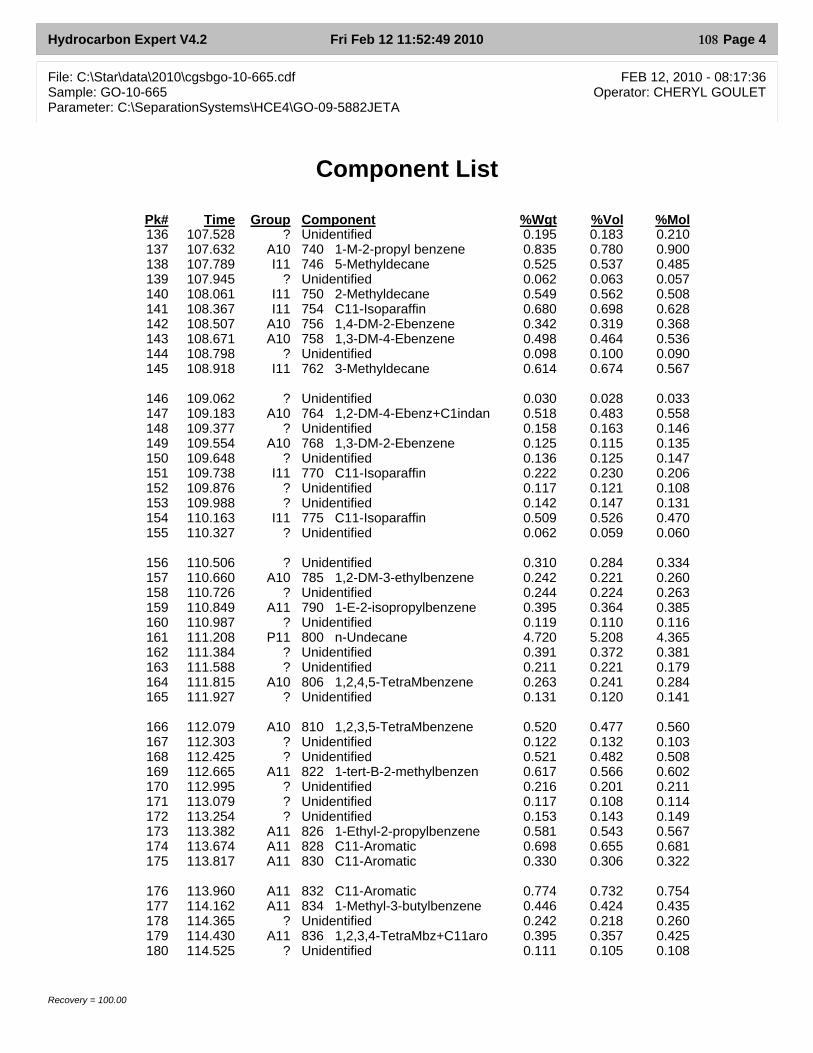
Hydrocarbon Expert V4.2 Fri Feb 12 11:52:49 2010 Page 4

File: C:\Star\data\2010\cgsbgo-10-665.cdf FEB 12, 2010 - 08:17:36Sample: GO-10-665 Operator: CHERYL GOULETParameter: C:\SeparationSystems\HCE4\GO-09-5882JETA

Component List

Recovery = 100.00

Pk# Time Group Component %Wgt %Vol %Mol136 107.528 ? Unidentified 0.195 0.183 0.210137 107.632 A10 740 1-M-2-propyl benzene 0.835 0.780 0.900138 107.789 I11 746 5-Methyldecane 0.525 0.537 0.485139 107.945 ? Unidentified 0.062 0.063 0.057140 108.061 I11 750 2-Methyldecane 0.549 0.562 0.508141 108.367 I11 754 C11-Isoparaffin 0.680 0.698 0.628142 108.507 A10 756 1,4-DM-2-Ebenzene 0.342 0.319 0.368143 108.671 A10 758 1,3-DM-4-Ebenzene 0.498 0.464 0.536144 108.798 ? Unidentified 0.098 0.100 0.090145 108.918 I11 762 3-Methyldecane 0.614 0.674 0.567

146 109.062 ? Unidentified 0.030 0.028 0.033147 109.183 A10 764 1,2-DM-4-Ebenz+C1indan 0.518 0.483 0.558148 109.377 ? Unidentified 0.158 0.163 0.146149 109.554 A10 768 1,3-DM-2-Ebenzene 0.125 0.115 0.135150 109.648 ? Unidentified 0.136 0.125 0.147151 109.738 I11 770 C11-Isoparaffin 0.222 0.230 0.206152 109.876 ? Unidentified 0.117 0.121 0.108153 109.988 ? Unidentified 0.142 0.147 0.131154 110.163 I11 775 C11-Isoparaffin 0.509 0.526 0.470155 110.327 ? Unidentified 0.062 0.059 0.060

156 110.506 ? Unidentified 0.310 0.284 0.334157 110.660 A10 785 1,2-DM-3-ethylbenzene 0.242 0.221 0.260158 110.726 ? Unidentified 0.244 0.224 0.263159 110.849 A11 790 1-E-2-isopropylbenzene 0.395 0.364 0.385160 110.987 ? Unidentified 0.119 0.110 0.116161 111.208 P11 800 n-Undecane 4.720 5.208 4.365162 111.384 ? Unidentified 0.391 0.372 0.381163 111.588 ? Unidentified 0.211 0.221 0.179164 111.815 A10 806 1,2,4,5-TetraMbenzene 0.263 0.241 0.284165 111.927 ? Unidentified 0.131 0.120 0.141

166 112.079 A10 810 1,2,3,5-TetraMbenzene 0.520 0.477 0.560167 112.303 ? Unidentified 0.122 0.132 0.103168 112.425 ? Unidentified 0.521 0.482 0.508169 112.665 A11 822 1-tert-B-2-methylbenzen 0.617 0.566 0.602170 112.995 ? Unidentified 0.216 0.201 0.211171 113.079 ? Unidentified 0.117 0.108 0.114172 113.254 ? Unidentified 0.153 0.143 0.149173 113.382 A11 826 1-Ethyl-2-propylbenzene 0.581 0.543 0.567174 113.674 A11 828 C11-Aromatic 0.698 0.655 0.681175 113.817 A11 830 C11-Aromatic 0.330 0.306 0.322

176 113.960 A11 832 C11-Aromatic 0.774 0.732 0.754177 114.162 A11 834 1-Methyl-3-butylbenzene 0.446 0.424 0.435178 114.365 ? Unidentified 0.242 0.218 0.260179 114.430 A11 836 1,2,3,4-TetraMbz+C11aro 0.395 0.357 0.425180 114.525 ? Unidentified 0.111 0.105 0.108

108

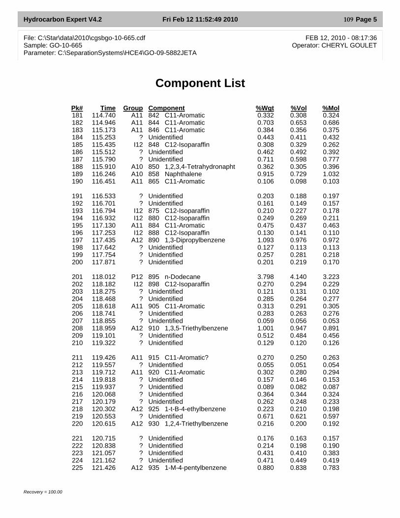
Hydrocarbon Expert V4.2 Fri Feb 12 11:52:49 2010 Page 5

File: C:\Star\data\2010\cgsbgo-10-665.cdf FEB 12, 2010 - 08:17:36Sample: GO-10-665 Operator: CHERYL GOULETParameter: C:\SeparationSystems\HCE4\GO-09-5882JETA

Component List

Recovery = 100.00

Pk# Time Group Component %Wgt %Vol %Mol181 114.740 A11 842 C11-Aromatic 0.332 0.308 0.324182 114.946 A11 844 C11-Aromatic 0.703 0.653 0.686183 115.173 A11 846 C11-Aromatic 0.384 0.356 0.375184 115.253 ? Unidentified 0.443 0.411 0.432185 115.435 I12 848 C12-Isoparaffin 0.308 0.329 0.262186 115.512 ? Unidentified 0.462 0.492 0.392187 115.790 ? Unidentified 0.711 0.598 0.777188 115.910 A10 850 1,2,3,4-Tetrahydronapht 0.362 0.305 0.396189 116.246 A10 858 Naphthalene 0.915 0.729 1.032190 116.451 A11 865 C11-Aromatic 0.106 0.098 0.103

191 116.533 ? Unidentified 0.203 0.188 0.197192 116.701 ? Unidentified 0.161 0.149 0.157193 116.794 I12 875 C12-Isoparaffin 0.210 0.227 0.178194 116.932 I12 880 C12-Isoparaffin 0.249 0.269 0.211195 117.130 A11 884 C11-Aromatic 0.475 0.437 0.463196 117.253 I12 888 C12-Isoparaffin 0.130 0.141 0.110197 117.435 A12 890 1,3-Dipropylbenzene 1.093 0.976 0.972198 117.642 ? Unidentified 0.127 0.113 0.113199 117.754 ? Unidentified 0.257 0.281 0.218200 117.871 ? Unidentified 0.201 0.219 0.170

201 118.012 P12 895 n-Dodecane 3.798 4.140 3.223202 118.182 I12 898 C12-Isoparaffin 0.270 0.294 0.229203 118.275 ? Unidentified 0.121 0.131 0.102204 118.468 ? Unidentified 0.285 0.264 0.277205 118.618 A11 905 C11-Aromatic 0.313 0.291 0.305206 118.741 ? Unidentified 0.283 0.263 0.276207 118.855 ? Unidentified 0.059 0.056 0.053208 118.959 A12 910 1,3,5-Triethylbenzene 1.001 0.947 0.891209 119.101 ? Unidentified 0.512 0.484 0.456210 119.322 ? Unidentified 0.129 0.120 0.126

211 119.426 A11 915 C11-Aromatic? 0.270 0.250 0.263212 119.557 ? Unidentified 0.055 0.051 0.054213 119.712 A11 920 C11-Aromatic 0.302 0.280 0.294214 119.818 ? Unidentified 0.157 0.146 0.153215 119.937 ? Unidentified 0.089 0.082 0.087216 120.068 ? Unidentified 0.364 0.344 0.324217 120.179 ? Unidentified 0.262 0.248 0.233218 120.302 A12 925 1-t-B-4-ethylbenzene 0.223 0.210 0.198219 120.553 ? Unidentified 0.671 0.621 0.597220 120.615 A12 930 1,2,4-Triethylbenzene 0.216 0.200 0.192

221 120.715 ? Unidentified 0.176 0.163 0.157222 120.838 ? Unidentified 0.214 0.198 0.190223 121.057 ? Unidentified 0.431 0.410 0.383224 121.162 ? Unidentified 0.471 0.449 0.419225 121.426 A12 935 1-M-4-pentylbenzene 0.880 0.838 0.783

109

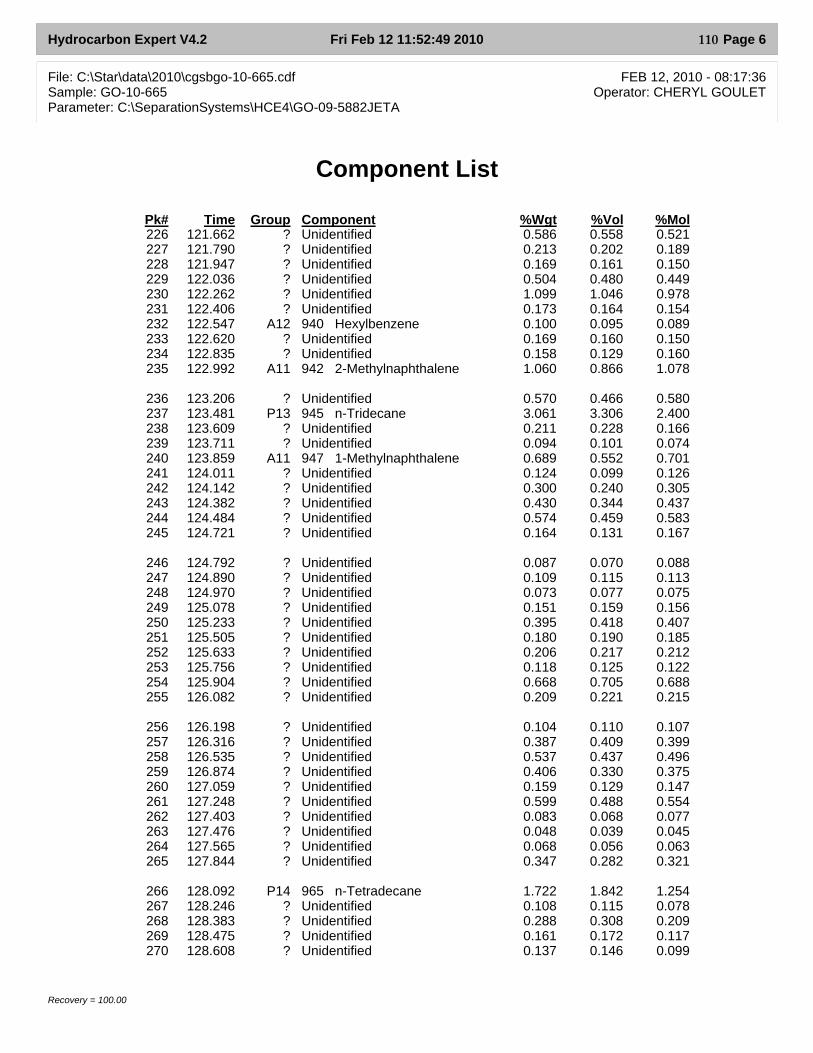
Hydrocarbon Expert V4.2 Fri Feb 12 11:52:49 2010 Page 6

File: C:\Star\data\2010\cgsbgo-10-665.cdf FEB 12, 2010 - 08:17:36Sample: GO-10-665 Operator: CHERYL GOULETParameter: C:\SeparationSystems\HCE4\GO-09-5882JETA

Component List

Recovery = 100.00

Pk# Time Group Component %Wgt %Vol %Mol226 121.662 ? Unidentified 0.586 0.558 0.521227 121.790 ? Unidentified 0.213 0.202 0.189228 121.947 ? Unidentified 0.169 0.161 0.150229 122.036 ? Unidentified 0.504 0.480 0.449230 122.262 ? Unidentified 1.099 1.046 0.978231 122.406 ? Unidentified 0.173 0.164 0.154232 122.547 A12 940 Hexylbenzene 0.100 0.095 0.089233 122.620 ? Unidentified 0.169 0.160 0.150234 122.835 ? Unidentified 0.158 0.129 0.160235 122.992 A11 942 2-Methylnaphthalene 1.060 0.866 1.078

236 123.206 ? Unidentified 0.570 0.466 0.580237 123.481 P13 945 n-Tridecane 3.061 3.306 2.400238 123.609 ? Unidentified 0.211 0.228 0.166239 123.711 ? Unidentified 0.094 0.101 0.074240 123.859 A11 947 1-Methylnaphthalene 0.689 0.552 0.701241 124.011 ? Unidentified 0.124 0.099 0.126242 124.142 ? Unidentified 0.300 0.240 0.305243 124.382 ? Unidentified 0.430 0.344 0.437244 124.484 ? Unidentified 0.574 0.459 0.583245 124.721 ? Unidentified 0.164 0.131 0.167

246 124.792 ? Unidentified 0.087 0.070 0.088247 124.890 ? Unidentified 0.109 0.115 0.113248 124.970 ? Unidentified 0.073 0.077 0.075249 125.078 ? Unidentified 0.151 0.159 0.156250 125.233 ? Unidentified 0.395 0.418 0.407251 125.505 ? Unidentified 0.180 0.190 0.185252 125.633 ? Unidentified 0.206 0.217 0.212253 125.756 ? Unidentified 0.118 0.125 0.122254 125.904 ? Unidentified 0.668 0.705 0.688255 126.082 ? Unidentified 0.209 0.221 0.215

256 126.198 ? Unidentified 0.104 0.110 0.107257 126.316 ? Unidentified 0.387 0.409 0.399258 126.535 ? Unidentified 0.537 0.437 0.496259 126.874 ? Unidentified 0.406 0.330 0.375260 127.059 ? Unidentified 0.159 0.129 0.147261 127.248 ? Unidentified 0.599 0.488 0.554262 127.403 ? Unidentified 0.083 0.068 0.077263 127.476 ? Unidentified 0.048 0.039 0.045264 127.565 ? Unidentified 0.068 0.056 0.063265 127.844 ? Unidentified 0.347 0.282 0.321

266 128.092 P14 965 n-Tetradecane 1.722 1.842 1.254267 128.246 ? Unidentified 0.108 0.115 0.078268 128.383 ? Unidentified 0.288 0.308 0.209269 128.475 ? Unidentified 0.161 0.172 0.117270 128.608 ? Unidentified 0.137 0.146 0.099

110

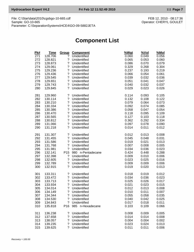
Hydrocarbon Expert V4.2 Fri Feb 12 11:52:49 2010 Page 7

File: C:\Star\data\2010\cgsbgo-10-665.cdf FEB 12, 2010 - 08:17:36Sample: GO-10-665 Operator: CHERYL GOULETParameter: C:\SeparationSystems\HCE4\GO-09-5882JETA

Component List

Recovery = 100.00

Pk# Time Group Component %Wgt %Vol %Mol271 128.706 ? Unidentified 0.060 0.049 0.056272 128.821 ? Unidentified 0.065 0.053 0.060273 128.873 ? Unidentified 0.086 0.070 0.079274 129.061 ? Unidentified 0.329 0.268 0.304275 129.236 ? Unidentified 0.237 0.193 0.219276 129.436 ? Unidentified 0.066 0.054 0.061277 129.545 ? Unidentified 0.039 0.032 0.036278 129.651 ? Unidentified 0.051 0.041 0.047279 129.743 ? Unidentified 0.040 0.032 0.037280 129.845 ? Unidentified 0.029 0.023 0.026

281 129.960 ? Unidentified 0.114 0.093 0.105282 130.114 ? Unidentified 0.132 0.108 0.122283 130.210 ? Unidentified 0.079 0.064 0.073284 130.334 ? Unidentified 0.092 0.074 0.085285 130.386 ? Unidentified 0.058 0.047 0.054286 130.470 ? Unidentified 0.118 0.095 0.109287 130.565 ? Unidentified 0.127 0.103 0.118288 130.812 ? Unidentified 0.362 0.292 0.334289 131.066 ? Unidentified 0.097 0.078 0.090290 131.218 ? Unidentified 0.014 0.011 0.012

291 131.307 ? Unidentified 0.012 0.013 0.008292 131.455 ? Unidentified 0.045 0.048 0.031293 131.586 ? Unidentified 0.019 0.021 0.013294 131.768 ? Unidentified 0.007 0.008 0.005295 131.981 ? Unidentified 0.034 0.036 0.023296 132.141 P15 980 n-Pentadecane 0.424 0.448 0.288297 132.398 ? Unidentified 0.009 0.010 0.006298 132.605 ? Unidentified 0.023 0.025 0.016299 132.789 ? Unidentified 0.009 0.009 0.006300 132.915 ? Unidentified 0.019 0.020 0.013

301 133.311 ? Unidentified 0.018 0.019 0.012302 133.472 ? Unidentified 0.034 0.036 0.023303 133.713 ? Unidentified 0.025 0.026 0.017304 133.934 ? Unidentified 0.021 0.023 0.015305 134.014 ? Unidentified 0.012 0.013 0.008306 134.149 ? Unidentified 0.010 0.011 0.007307 134.344 ? Unidentified 0.055 0.058 0.035308 134.530 ? Unidentified 0.040 0.042 0.025309 134.843 ? Unidentified 0.017 0.018 0.011310 135.818 P16 985 n-Hexadecane 0.103 0.109 0.066

311 136.238 ? Unidentified 0.008 0.009 0.005312 137.658 ? Unidentified 0.014 0.014 0.008313 138.057 ? Unidentified 0.004 0.004 0.002314 139.235 ? Unidentified 0.023 0.024 0.013315 139.625 ? Unidentified 0.011 0.011 0.006

111

Hydrocarbon Expert V4.2 Fri Feb 12 11:52:49 2010 Page 8

File: C:\Star\data\2010\cgsbgo-10-665.cdf FEB 12, 2010 - 08:17:36Sample: GO-10-665 Operator: CHERYL GOULETParameter: C:\SeparationSystems\HCE4\GO-09-5882JETA

Component List

Recovery = 100.00

Pk# Time Group Component %Wgt %Vol %Mol

112

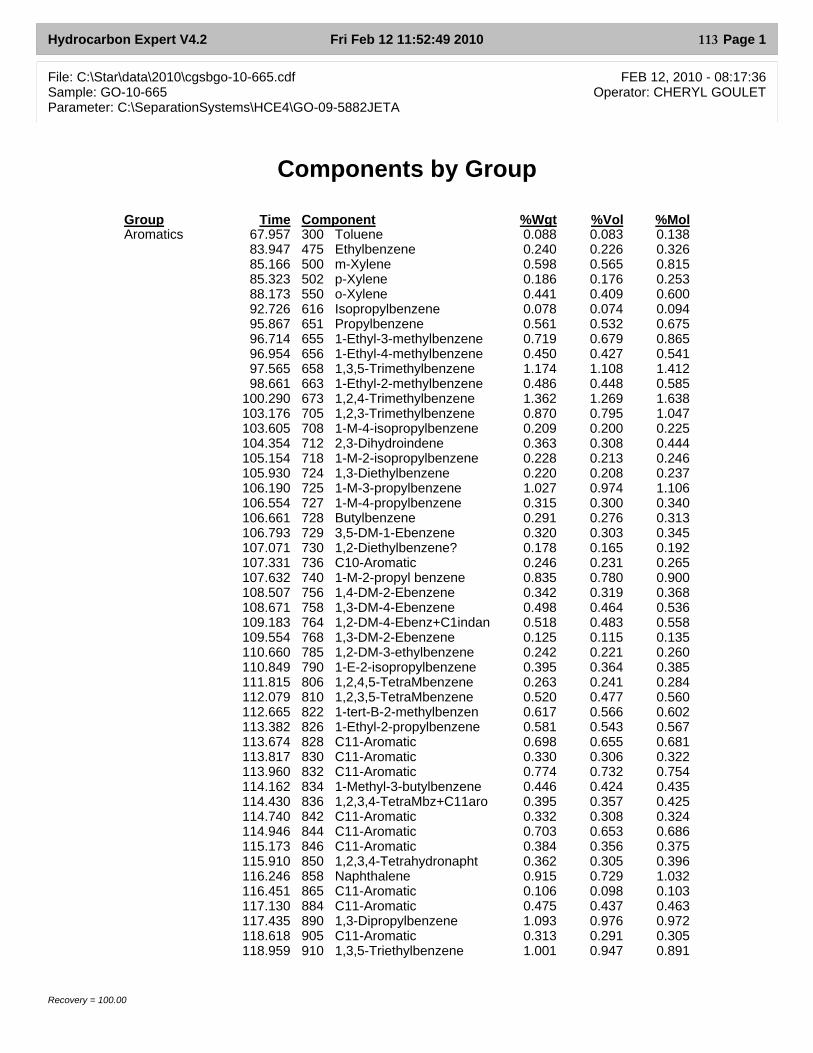
Hydrocarbon Expert V4.2 Fri Feb 12 11:52:49 2010 Page 1

File: C:\Star\data\2010\cgsbgo-10-665.cdf FEB 12, 2010 - 08:17:36Sample: GO-10-665 Operator: CHERYL GOULETParameter: C:\SeparationSystems\HCE4\GO-09-5882JETA

Components by Group

Recovery = 100.00

Group Time Component %Wgt %Vol %MolAromatics 67.957 300 Toluene 0.088 0.083 0.138

83.947 475 Ethylbenzene 0.240 0.226 0.32685.166 500 m-Xylene 0.598 0.565 0.81585.323 502 p-Xylene 0.186 0.176 0.25388.173 550 o-Xylene 0.441 0.409 0.60092.726 616 Isopropylbenzene 0.078 0.074 0.09495.867 651 Propylbenzene 0.561 0.532 0.67596.714 655 1-Ethyl-3-methylbenzene 0.719 0.679 0.86596.954 656 1-Ethyl-4-methylbenzene 0.450 0.427 0.54197.565 658 1,3,5-Trimethylbenzene 1.174 1.108 1.41298.661 663 1-Ethyl-2-methylbenzene 0.486 0.448 0.585

100.290 673 1,2,4-Trimethylbenzene 1.362 1.269 1.638103.176 705 1,2,3-Trimethylbenzene 0.870 0.795 1.047103.605 708 1-M-4-isopropylbenzene 0.209 0.200 0.225104.354 712 2,3-Dihydroindene 0.363 0.308 0.444105.154 718 1-M-2-isopropylbenzene 0.228 0.213 0.246105.930 724 1,3-Diethylbenzene 0.220 0.208 0.237106.190 725 1-M-3-propylbenzene 1.027 0.974 1.106106.554 727 1-M-4-propylbenzene 0.315 0.300 0.340106.661 728 Butylbenzene 0.291 0.276 0.313106.793 729 3,5-DM-1-Ebenzene 0.320 0.303 0.345107.071 730 1,2-Diethylbenzene? 0.178 0.165 0.192107.331 736 C10-Aromatic 0.246 0.231 0.265107.632 740 1-M-2-propyl benzene 0.835 0.780 0.900108.507 756 1,4-DM-2-Ebenzene 0.342 0.319 0.368108.671 758 1,3-DM-4-Ebenzene 0.498 0.464 0.536109.183 764 1,2-DM-4-Ebenz+C1indan 0.518 0.483 0.558109.554 768 1,3-DM-2-Ebenzene 0.125 0.115 0.135110.660 785 1,2-DM-3-ethylbenzene 0.242 0.221 0.260110.849 790 1-E-2-isopropylbenzene 0.395 0.364 0.385111.815 806 1,2,4,5-TetraMbenzene 0.263 0.241 0.284112.079 810 1,2,3,5-TetraMbenzene 0.520 0.477 0.560112.665 822 1-tert-B-2-methylbenzen 0.617 0.566 0.602113.382 826 1-Ethyl-2-propylbenzene 0.581 0.543 0.567113.674 828 C11-Aromatic 0.698 0.655 0.681113.817 830 C11-Aromatic 0.330 0.306 0.322113.960 832 C11-Aromatic 0.774 0.732 0.754114.162 834 1-Methyl-3-butylbenzene 0.446 0.424 0.435114.430 836 1,2,3,4-TetraMbz+C11aro 0.395 0.357 0.425114.740 842 C11-Aromatic 0.332 0.308 0.324114.946 844 C11-Aromatic 0.703 0.653 0.686115.173 846 C11-Aromatic 0.384 0.356 0.375115.910 850 1,2,3,4-Tetrahydronapht 0.362 0.305 0.396116.246 858 Naphthalene 0.915 0.729 1.032116.451 865 C11-Aromatic 0.106 0.098 0.103117.130 884 C11-Aromatic 0.475 0.437 0.463117.435 890 1,3-Dipropylbenzene 1.093 0.976 0.972118.618 905 C11-Aromatic 0.313 0.291 0.305118.959 910 1,3,5-Triethylbenzene 1.001 0.947 0.891

113

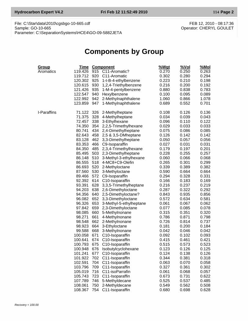
Hydrocarbon Expert V4.2 Fri Feb 12 11:52:49 2010 Page 2

File: C:\Star\data\2010\cgsbgo-10-665.cdf FEB 12, 2010 - 08:17:36Sample: GO-10-665 Operator: CHERYL GOULETParameter: C:\SeparationSystems\HCE4\GO-09-5882JETA

Components by Group

Recovery = 100.00

Group Time Component %Wgt %Vol %MolAromatics 119.426 915 C11-Aromatic? 0.270 0.250 0.263

119.712 920 C11-Aromatic 0.302 0.280 0.294120.302 925 1-t-B-4-ethylbenzene 0.223 0.210 0.198120.615 930 1,2,4-Triethylbenzene 0.216 0.200 0.192121.426 935 1-M-4-pentylbenzene 0.880 0.838 0.783122.547 940 Hexylbenzene 0.100 0.095 0.089122.992 942 2-Methylnaphthalene 1.060 0.866 1.078123.859 947 1-Methylnaphthalene 0.689 0.552 0.701

I-Paraffins 71.122 326 2-Methylheptane 0.108 0.126 0.13671.375 328 4-Methylheptane 0.034 0.039 0.04372.457 338 3-Ethylhexane 0.096 0.110 0.12274.350 354 2,2,5-Trimethylhexane 0.029 0.033 0.03380.741 434 2,4-Dimethylheptane 0.075 0.086 0.08582.643 458 2,5 & 3,5-DMheptane 0.126 0.142 0.14283.128 462 3,3-Dimethylheptane 0.050 0.057 0.05683.353 466 C9-Isoparaffin 0.027 0.031 0.03184.350 485 2,3,4-Trimethylhexane 0.179 0.197 0.20185.495 503 2,3-Dimethylheptane 0.228 0.255 0.25786.148 510 3-Methyl-3-ethylhexane 0.060 0.066 0.06886.555 518 4-MC8+C9-Olefin 0.265 0.301 0.29986.693 520 2-Methyloctane 0.339 0.389 0.38287.560 530 3-Methyloctane 0.590 0.664 0.66489.466 572 C9-Isoparaffin 0.294 0.328 0.33192.392 614 C10-Isoparaffin 0.166 0.183 0.16993.391 628 3,3,5-Trimethylheptane 0.216 0.237 0.21994.203 638 2,6-Dimethyloctane 0.287 0.322 0.29294.356 640 2,5-Dimethyloctane? 0.843 0.935 0.85696.082 652 3,3-Dimethyloctane 0.572 0.634 0.58196.326 653 3-Methyl-5-ethylheptane 0.061 0.067 0.06297.842 659 2,3-Dimethyloctane 0.077 0.085 0.07898.085 660 5-Methylnonane 0.315 0.351 0.32098.271 661 4-Methylnonane 0.786 0.871 0.79898.548 662 2-Methylnonane 0.726 0.814 0.73798.923 664 3-Ethyloctane 0.181 0.200 0.18499.588 668 3-Methylnonane 0.042 0.046 0.042

100.058 671 C10-Isoparaffin 0.092 0.102 0.093100.641 674 C10-Isoparaffin 0.415 0.461 0.421100.793 675 C10-Isoparaffin 0.515 0.573 0.523100.948 676 Isobutylcyclohexane 0.123 0.126 0.125101.241 677 C10-Isoparaffin 0.124 0.138 0.126101.922 702 C11-Isoparaffin 0.344 0.381 0.318102.591 704 C11-Isoparaffin 0.063 0.070 0.058103.796 709 C11-Isoparaffin 0.327 0.361 0.302105.019 716 C11-isoParrafin 0.061 0.068 0.057105.743 723 C11-Isoparaffin 0.673 0.731 0.622107.789 746 5-Methyldecane 0.525 0.537 0.485108.061 750 2-Methyldecane 0.549 0.562 0.508108.367 754 C11-Isoparaffin 0.680 0.698 0.628

114

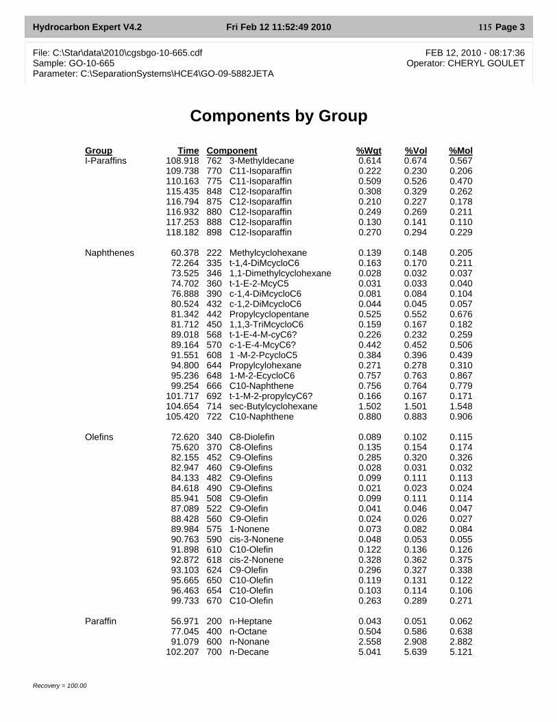
Hydrocarbon Expert V4.2 Fri Feb 12 11:52:49 2010 Page 3

File: C:\Star\data\2010\cgsbgo-10-665.cdf FEB 12, 2010 - 08:17:36Sample: GO-10-665 Operator: CHERYL GOULETParameter: C:\SeparationSystems\HCE4\GO-09-5882JETA

Components by Group

Recovery = 100.00

Group Time Component %Wgt %Vol %MolI-Paraffins 108.918 762 3-Methyldecane 0.614 0.674 0.567

109.738 770 C11-Isoparaffin 0.222 0.230 0.206110.163 775 C11-Isoparaffin 0.509 0.526 0.470115.435 848 C12-Isoparaffin 0.308 0.329 0.262116.794 875 C12-Isoparaffin 0.210 0.227 0.178116.932 880 C12-Isoparaffin 0.249 0.269 0.211117.253 888 C12-Isoparaffin 0.130 0.141 0.110118.182 898 C12-Isoparaffin 0.270 0.294 0.229

Naphthenes 60.378 222 Methylcyclohexane 0.139 0.148 0.20572.264 335 t-1,4-DiMcycloC6 0.163 0.170 0.21173.525 346 1,1-Dimethylcyclohexane 0.028 0.032 0.03774.702 360 t-1-E-2-McyC5 0.031 0.033 0.04076.888 390 c-1,4-DiMcycloC6 0.081 0.084 0.10480.524 432 c-1,2-DiMcycloC6 0.044 0.045 0.05781.342 442 Propylcyclopentane 0.525 0.552 0.67681.712 450 1,1,3-TriMcycloC6 0.159 0.167 0.18289.018 568 t-1-E-4-M-cyC6? 0.226 0.232 0.25989.164 570 c-1-E-4-McyC6? 0.442 0.452 0.50691.551 608 1 -M-2-PcycloC5 0.384 0.396 0.43994.800 644 Propylcylohexane 0.271 0.278 0.31095.236 648 1-M-2-EcycloC6 0.757 0.763 0.86799.254 666 C10-Naphthene 0.756 0.764 0.779

101.717 692 t-1-M-2-propylcyC6? 0.166 0.167 0.171104.654 714 sec-Butylcyclohexane 1.502 1.501 1.548105.420 722 C10-Naphthene 0.880 0.883 0.906

Olefins 72.620 340 C8-Diolefin 0.089 0.102 0.11575.620 370 C8-Olefins 0.135 0.154 0.17482.155 452 C9-Olefins 0.285 0.320 0.32682.947 460 C9-Olefins 0.028 0.031 0.03284.133 482 C9-Olefins 0.099 0.111 0.11384.618 490 C9-Olefins 0.021 0.023 0.02485.941 508 C9-Olefin 0.099 0.111 0.11487.089 522 C9-Olefin 0.041 0.046 0.04788.428 560 C9-Olefin 0.024 0.026 0.02789.984 575 1-Nonene 0.073 0.082 0.08490.763 590 cis-3-Nonene 0.048 0.053 0.05591.898 610 C10-Olefin 0.122 0.136 0.12692.872 618 cis-2-Nonene 0.328 0.362 0.37593.103 624 C9-Olefin 0.296 0.327 0.33895.665 650 C10-Olefin 0.119 0.131 0.12296.463 654 C10-Olefin 0.103 0.114 0.10699.733 670 C10-Olefin 0.263 0.289 0.271

Paraffin 56.971 200 n-Heptane 0.043 0.051 0.06277.045 400 n-Octane 0.504 0.586 0.63891.079 600 n-Nonane 2.558 2.908 2.882

102.207 700 n-Decane 5.041 5.639 5.121

115

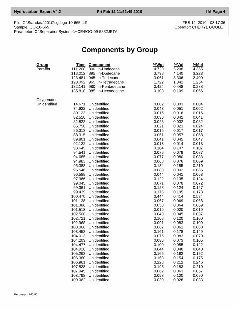
Hydrocarbon Expert V4.2 Fri Feb 12 11:52:49 2010 Page 4

File: C:\Star\data\2010\cgsbgo-10-665.cdf FEB 12, 2010 - 08:17:36Sample: GO-10-665 Operator: CHERYL GOULETParameter: C:\SeparationSystems\HCE4\GO-09-5882JETA

Components by Group

Recovery = 100.00

Group Time Component %Wgt %Vol %MolParaffin 111.208 800 n-Undecane 4.720 5.208 4.365

118.012 895 n-Dodecane 3.798 4.140 3.223123.481 945 n-Tridecane 3.061 3.306 2.400128.092 965 n-Tetradecane 1.722 1.842 1.254132.141 980 n-Pentadecane 0.424 0.448 0.288135.818 985 n-Hexadecane 0.103 0.109 0.066

OxygenatesUnidentified 14.671 Unidentified 0.002 0.003 0.004

74.922 Unidentified 0.048 0.051 0.06280.123 Unidentified 0.015 0.016 0.01682.510 Unidentified 0.036 0.041 0.04182.823 Unidentified 0.028 0.032 0.03285.750 Unidentified 0.021 0.023 0.02486.313 Unidentified 0.015 0.017 0.01788.315 Unidentified 0.051 0.057 0.05889.801 Unidentified 0.041 0.045 0.04792.122 Unidentified 0.013 0.014 0.01393.649 Unidentified 0.104 0.107 0.10794.541 Unidentified 0.076 0.079 0.08794.685 Unidentified 0.077 0.080 0.08894.983 Unidentified 0.068 0.076 0.06995.388 Unidentified 0.184 0.185 0.21095.546 Unidentified 0.083 0.092 0.08696.589 Unidentified 0.044 0.041 0.05397.966 Unidentified 0.122 0.135 0.12499.045 Unidentified 0.071 0.078 0.07299.361 Unidentified 0.123 0.124 0.12799.439 Unidentified 0.175 0.195 0.178

100.470 Unidentified 0.444 0.414 0.534101.138 Unidentified 0.067 0.069 0.068101.386 Unidentified 0.058 0.064 0.059101.518 Unidentified 0.019 0.020 0.019102.508 Unidentified 0.040 0.045 0.037102.721 Unidentified 0.108 0.120 0.100102.968 Unidentified 0.091 0.083 0.109103.066 Unidentified 0.067 0.061 0.080103.452 Unidentified 0.161 0.178 0.149104.013 Unidentified 0.075 0.083 0.070104.203 Unidentified 0.086 0.073 0.105104.477 Unidentified 0.100 0.085 0.122104.928 Unidentified 0.044 0.048 0.040105.263 Unidentified 0.165 0.182 0.152106.380 Unidentified 0.163 0.154 0.175106.961 Unidentified 0.228 0.212 0.246107.528 Unidentified 0.195 0.183 0.210107.945 Unidentified 0.062 0.063 0.057108.798 Unidentified 0.098 0.100 0.090109.062 Unidentified 0.030 0.028 0.033

116

Hydrocarbon Expert V4.2 Fri Feb 12 11:52:49 2010 Page 5

File: C:\Star\data\2010\cgsbgo-10-665.cdf FEB 12, 2010 - 08:17:36Sample: GO-10-665 Operator: CHERYL GOULETParameter: C:\SeparationSystems\HCE4\GO-09-5882JETA

Components by Group

Recovery = 100.00

Group Time Component %Wgt %Vol %MolUnidentified 109.377 Unidentified 0.158 0.163 0.146

109.648 Unidentified 0.136 0.125 0.147109.876 Unidentified 0.117 0.121 0.108109.988 Unidentified 0.142 0.147 0.131110.327 Unidentified 0.062 0.059 0.060110.506 Unidentified 0.310 0.284 0.334110.726 Unidentified 0.244 0.224 0.263110.987 Unidentified 0.119 0.110 0.116111.384 Unidentified 0.391 0.372 0.381111.588 Unidentified 0.211 0.221 0.179111.927 Unidentified 0.131 0.120 0.141112.303 Unidentified 0.122 0.132 0.103112.425 Unidentified 0.521 0.482 0.508112.995 Unidentified 0.216 0.201 0.211113.079 Unidentified 0.117 0.108 0.114113.254 Unidentified 0.153 0.143 0.149114.365 Unidentified 0.242 0.218 0.260114.525 Unidentified 0.111 0.105 0.108115.253 Unidentified 0.443 0.411 0.432115.512 Unidentified 0.462 0.492 0.392115.790 Unidentified 0.711 0.598 0.777116.533 Unidentified 0.203 0.188 0.197116.701 Unidentified 0.161 0.149 0.157117.642 Unidentified 0.127 0.113 0.113117.754 Unidentified 0.257 0.281 0.218117.871 Unidentified 0.201 0.219 0.170118.275 Unidentified 0.121 0.131 0.102118.468 Unidentified 0.285 0.264 0.277118.741 Unidentified 0.283 0.263 0.276118.855 Unidentified 0.059 0.056 0.053119.101 Unidentified 0.512 0.484 0.456119.322 Unidentified 0.129 0.120 0.126119.557 Unidentified 0.055 0.051 0.054119.818 Unidentified 0.157 0.146 0.153119.937 Unidentified 0.089 0.082 0.087120.068 Unidentified 0.364 0.344 0.324120.179 Unidentified 0.262 0.248 0.233120.553 Unidentified 0.671 0.621 0.597120.715 Unidentified 0.176 0.163 0.157120.838 Unidentified 0.214 0.198 0.190121.057 Unidentified 0.431 0.410 0.383121.162 Unidentified 0.471 0.449 0.419121.662 Unidentified 0.586 0.558 0.521121.790 Unidentified 0.213 0.202 0.189121.947 Unidentified 0.169 0.161 0.150122.036 Unidentified 0.504 0.480 0.449122.262 Unidentified 1.099 1.046 0.978122.406 Unidentified 0.173 0.164 0.154122.620 Unidentified 0.169 0.160 0.150

117

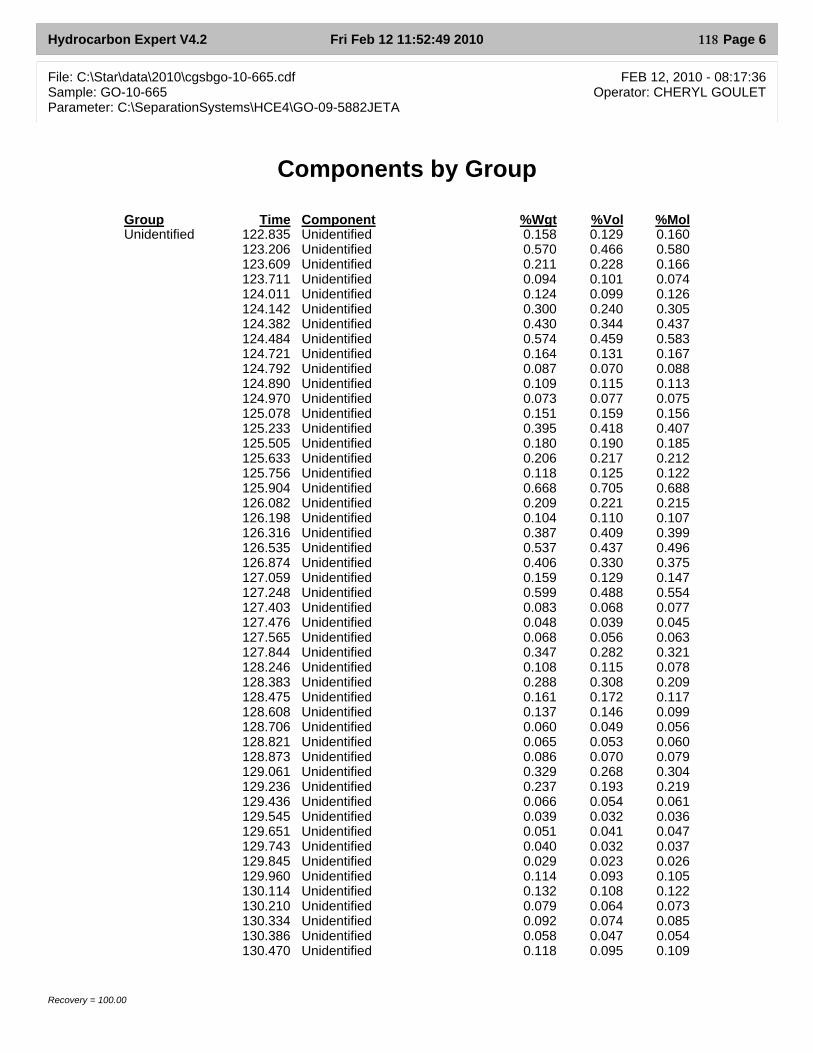
Hydrocarbon Expert V4.2 Fri Feb 12 11:52:49 2010 Page 6

File: C:\Star\data\2010\cgsbgo-10-665.cdf FEB 12, 2010 - 08:17:36Sample: GO-10-665 Operator: CHERYL GOULETParameter: C:\SeparationSystems\HCE4\GO-09-5882JETA

Components by Group

Recovery = 100.00

Group Time Component %Wgt %Vol %MolUnidentified 122.835 Unidentified 0.158 0.129 0.160

123.206 Unidentified 0.570 0.466 0.580123.609 Unidentified 0.211 0.228 0.166123.711 Unidentified 0.094 0.101 0.074124.011 Unidentified 0.124 0.099 0.126124.142 Unidentified 0.300 0.240 0.305124.382 Unidentified 0.430 0.344 0.437124.484 Unidentified 0.574 0.459 0.583124.721 Unidentified 0.164 0.131 0.167124.792 Unidentified 0.087 0.070 0.088124.890 Unidentified 0.109 0.115 0.113124.970 Unidentified 0.073 0.077 0.075125.078 Unidentified 0.151 0.159 0.156125.233 Unidentified 0.395 0.418 0.407125.505 Unidentified 0.180 0.190 0.185125.633 Unidentified 0.206 0.217 0.212125.756 Unidentified 0.118 0.125 0.122125.904 Unidentified 0.668 0.705 0.688126.082 Unidentified 0.209 0.221 0.215126.198 Unidentified 0.104 0.110 0.107126.316 Unidentified 0.387 0.409 0.399126.535 Unidentified 0.537 0.437 0.496126.874 Unidentified 0.406 0.330 0.375127.059 Unidentified 0.159 0.129 0.147127.248 Unidentified 0.599 0.488 0.554127.403 Unidentified 0.083 0.068 0.077127.476 Unidentified 0.048 0.039 0.045127.565 Unidentified 0.068 0.056 0.063127.844 Unidentified 0.347 0.282 0.321128.246 Unidentified 0.108 0.115 0.078128.383 Unidentified 0.288 0.308 0.209128.475 Unidentified 0.161 0.172 0.117128.608 Unidentified 0.137 0.146 0.099128.706 Unidentified 0.060 0.049 0.056128.821 Unidentified 0.065 0.053 0.060128.873 Unidentified 0.086 0.070 0.079129.061 Unidentified 0.329 0.268 0.304129.236 Unidentified 0.237 0.193 0.219129.436 Unidentified 0.066 0.054 0.061129.545 Unidentified 0.039 0.032 0.036129.651 Unidentified 0.051 0.041 0.047129.743 Unidentified 0.040 0.032 0.037129.845 Unidentified 0.029 0.023 0.026129.960 Unidentified 0.114 0.093 0.105130.114 Unidentified 0.132 0.108 0.122130.210 Unidentified 0.079 0.064 0.073130.334 Unidentified 0.092 0.074 0.085130.386 Unidentified 0.058 0.047 0.054130.470 Unidentified 0.118 0.095 0.109

118

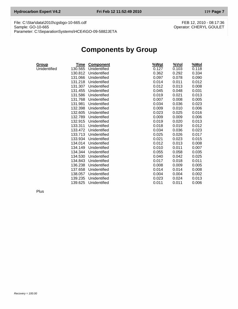
Hydrocarbon Expert V4.2 Fri Feb 12 11:52:49 2010 Page 7

File: C:\Star\data\2010\cgsbgo-10-665.cdf FEB 12, 2010 - 08:17:36Sample: GO-10-665 Operator: CHERYL GOULETParameter: C:\SeparationSystems\HCE4\GO-09-5882JETA

Components by Group

Recovery = 100.00

Group Time Component %Wgt %Vol %MolUnidentified 130.565 Unidentified 0.127 0.103 0.118

130.812 Unidentified 0.362 0.292 0.334131.066 Unidentified 0.097 0.078 0.090131.218 Unidentified 0.014 0.011 0.012131.307 Unidentified 0.012 0.013 0.008131.455 Unidentified 0.045 0.048 0.031131.586 Unidentified 0.019 0.021 0.013131.768 Unidentified 0.007 0.008 0.005131.981 Unidentified 0.034 0.036 0.023132.398 Unidentified 0.009 0.010 0.006132.605 Unidentified 0.023 0.025 0.016132.789 Unidentified 0.009 0.009 0.006132.915 Unidentified 0.019 0.020 0.013133.311 Unidentified 0.018 0.019 0.012133.472 Unidentified 0.034 0.036 0.023133.713 Unidentified 0.025 0.026 0.017133.934 Unidentified 0.021 0.023 0.015134.014 Unidentified 0.012 0.013 0.008134.149 Unidentified 0.010 0.011 0.007134.344 Unidentified 0.055 0.058 0.035134.530 Unidentified 0.040 0.042 0.025134.843 Unidentified 0.017 0.018 0.011136.238 Unidentified 0.008 0.009 0.005137.658 Unidentified 0.014 0.014 0.008138.057 Unidentified 0.004 0.004 0.002139.235 Unidentified 0.023 0.024 0.013139.625 Unidentified 0.011 0.011 0.006

Plus

119

Hydrocarbon Expert V4.2 Tue Feb 23 15:52:26 2010 Page 1

File: C:\Star\data\2010\cgsbgo-10-665.cdf FEB 12, 2010 - 08:17:36Sample: GO-10-665 Operator: CHERYL GOULETParameter: C:\SeparationSystems\HCE4\GO-09-5882JETA

Sample Chromatogram

C:\S

tar\data\2010\cgsbgo-10-665.cdf

128118

10898

8878

68 300 Toluene

475 Ethylbenzene500 m-Xylene502 p-Xylene

550 o-Xylene

616 Isopropylbenzene

651 Propylbenzene655 1-Ethyl-3-methylbenzene656 1-Ethyl-4-methylbenzene658 1,3,5-Trimethylbenzene

663 1-Ethyl-2-methylbenzene673 1,2,4-Trimethylbenzene

705 1,2,3-Trimethylbenzene708 1-M-4-isopropylbenzene712 2,3-Dihydroindene

718 1-M-2-isopropylbenzene724 1,3-Diethylbenzene725 1-M-3-propylbenzene727 1-M-4-propylbenzene728 Butylbenzene729 3,5-DM-1-Ebenzene730 1,2-Diethylbenzene?736 C10-Aromatic740 1-M-2-propyl benzene

756 1,4-DM-2-Ebenzene758 1,3-DM-4-Ebenzene764 1,2-DM-4-Ebenz+C1indan768 1,3-DM-2-Ebenzene785 1,2-DM-3-ethylbenzene790 1-E-2-isopropylbenzene806 1,2,4,5-TetraMbenzene810 1,2,3,5-TetraMbenzene822 1-tert-B-2-methylbenzen826 1-Ethyl-2-propylbenzene828 C11-Aromatic830 C11-Aromatic832 C11-Aromatic834 1-Methyl-3-butylbenzene836 1,2,3,4-TetraMbz+C11aro842 C11-Aromatic844 C11-Aromatic846 C11-Aromatic850 1,2,3,4-Tetrahydronapht858 Naphthalene865 C11-Aromatic884 C11-Aromatic890 1,3-Dipropylbenzene905 C11-Aromatic 910 1,3,5-Triethylbenzene915 C11-Aromatic?920 C11-Aromatic925 1-t-B-4-ethylbenzene930 1,2,4-Triethylbenzene

935 1-M-4-pentylbenzene940 Hexylbenzene 942 2-Methylnaphthalene

947 1-Methylnaphthalene

120

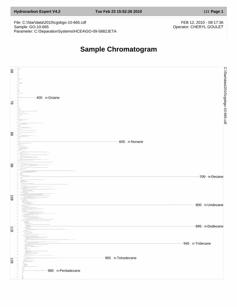
Hydrocarbon Expert V4.2 Tue Feb 23 15:52:26 2010 Page 1

File: C:\Star\data\2010\cgsbgo-10-665.cdf FEB 12, 2010 - 08:17:36Sample: GO-10-665 Operator: CHERYL GOULETParameter: C:\SeparationSystems\HCE4\GO-09-5882JETA

Sample Chromatogram

C:\S

tar\data\2010\cgsbgo-10-665.cdf

128118

10898

8878

68

400 n-Octane

600 n-Nonane

700 n-Decane

800 n-Undecane

895 n-Dodecane

945 n-Tridecane

965 n-Tetradecane

980 n-Pentadecane

121

Appendix A

Part II:

Jet Fuels Thermophysical Properties

Fuels are:

A: Sasol CTL

B: Shell GTL

C: 50 vol.% Shell GTL + 50 vol.% Naphthenic compounds

D: 80 vol.% Shell GTL + 20 vol.% Hexanol

E: Jet A-1

122

TPRL 4453

Thermophysical Properties of Jet Fuel

A Report to University of Toronto

by

J. Gembarovic and J. Freeman

February 2010

TPRL, Inc. 3080 Kent Avenue

West Lafayette, IN 47906 Phone: 765-463-1581

Fax: 765-463-5235

WWW.TPRL.COM

123

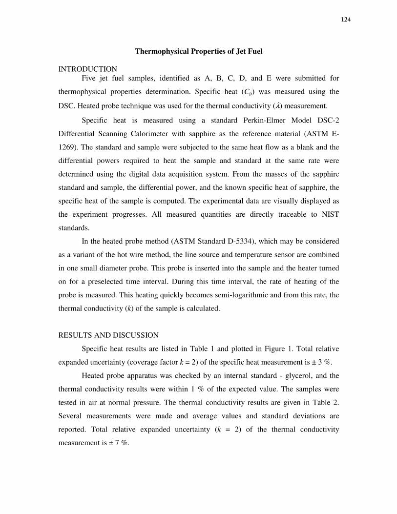
Thermophysical Properties of Jet Fuel

INTRODUCTION

Five jet fuel samples, identified as A, B, C, D, and E were submitted for

thermophysical properties determination. Specific heat (Cp) was measured using the

DSC. Heated probe technique was used for the thermal conductivity (λ) measurement.

Specific heat is measured using a standard Perkin-Elmer Model DSC-2

Differential Scanning Calorimeter with sapphire as the reference material (ASTM E-

1269). The standard and sample were subjected to the same heat flow as a blank and the

differential powers required to heat the sample and standard at the same rate were

determined using the digital data acquisition system. From the masses of the sapphire

standard and sample, the differential power, and the known specific heat of sapphire, the

specific heat of the sample is computed. The experimental data are visually displayed as

the experiment progresses. All measured quantities are directly traceable to NIST

standards.

In the heated probe method (ASTM Standard D-5334), which may be considered

as a variant of the hot wire method, the line source and temperature sensor are combined

in one small diameter probe. This probe is inserted into the sample and the heater turned

on for a preselected time interval. During this time interval, the rate of heating of the

probe is measured. This heating quickly becomes semi-logarithmic and from this rate, the

thermal conductivity (k) of the sample is calculated.

RESULTS AND DISCUSSION

Specific heat results are listed in Table 1 and plotted in Figure 1. Total relative

expanded uncertainty (coverage factor k = 2) of the specific heat measurement is ± 3 %.

Heated probe apparatus was checked by an internal standard - glycerol, and the

thermal conductivity results were within 1 % of the expected value. The samples were

tested in air at normal pressure. The thermal conductivity results are given in Table 2.

Several measurements were made and average values and standard deviations are

reported. Total relative expanded uncertainty (k = 2) of the thermal conductivity

measurement is ± 7 %.

124

2

Table 1 Specific Heat Results

T/C

A B C D E

23 1.95 2.13 2.00 2.35 1.91

40 2.02 2.24 2.10 2.41 2.00

60 2.11 2.34 2.21 2.46 2.09

80 2.19 2.39 2.29 2.48 2.17

100 2.26 2.45 2.35 2.51 2.23

Cp / (J/g K)

Table 2 Thermal Conductivity Results

T/C

A B C D E

23 0.138 0.149 0.127 0.145 0.140

23 0.133 0.149 0.134 0.147 0.137

23 0.133 0.147 0.130 0.147 0.135

Average 0.135 0.148 0.130 0.146 0.137

STDEV 0.003 0.001 0.004 0.001 0.003

Thermal Conductivity / (W/m K)

1.7

1.8

1.9

2.0

2.1

2.2

2.3

2.4

2.5

2.6

20 30 40 50 60 70 80 90 100 110

T/C

Cp /

(J/g

K)

A

B

C

D

E

Figure 1 Specific Heat

125

Appendix A

Part III:

Jet A-1 Thermodynamic Properties

126

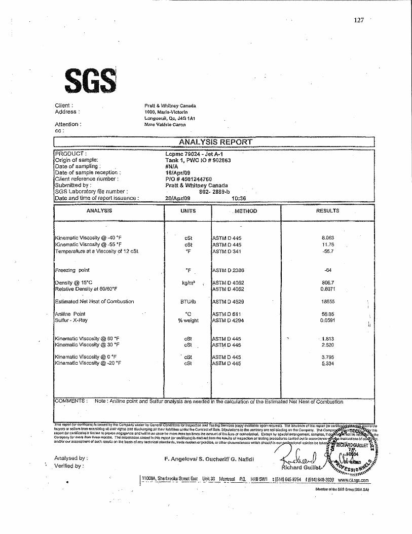
127

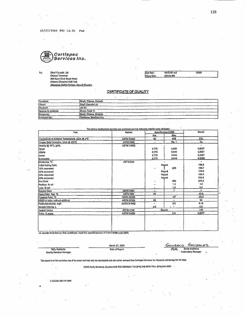
128

Appendix B

Step by Step Sample Analysis on GC-TCD

129

130

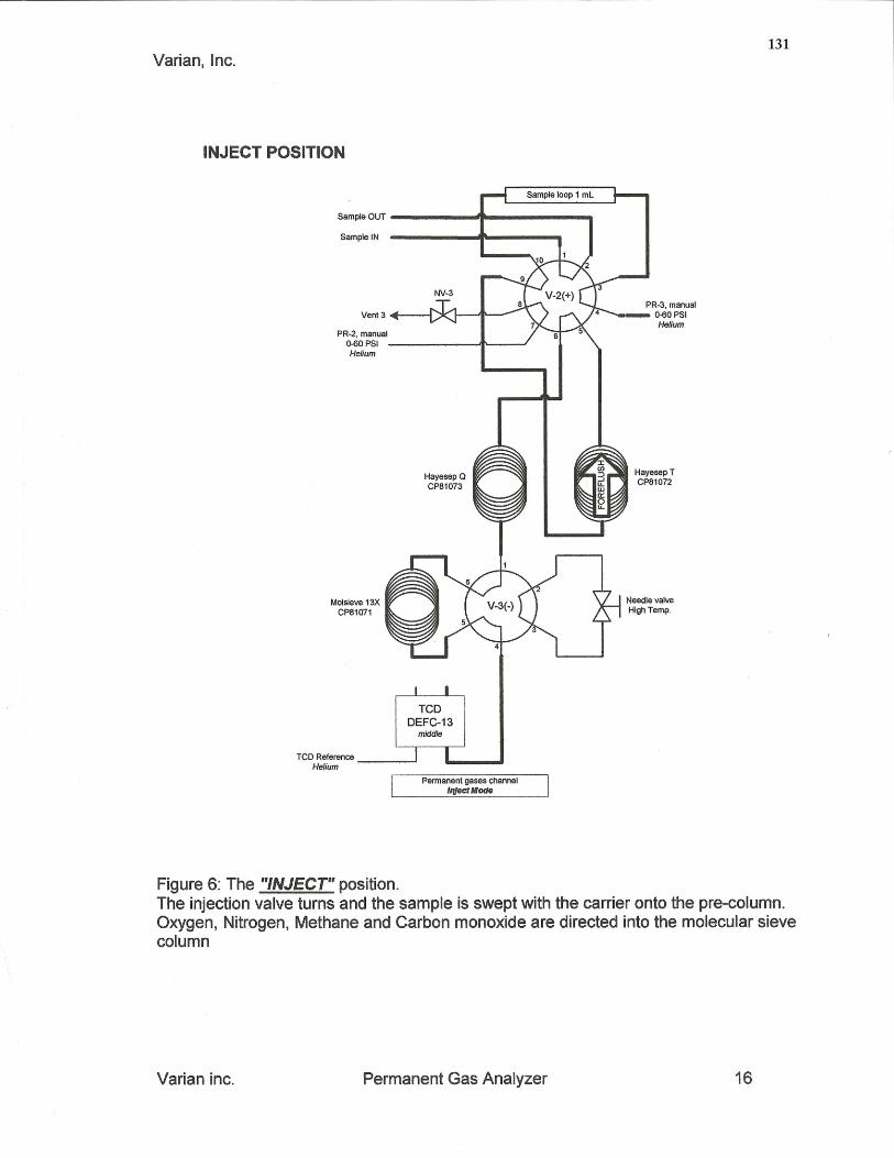
131

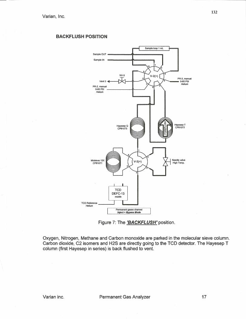
132

Appendix C

Sample Gas Chromatograms

133

134

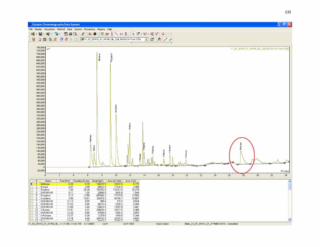
135

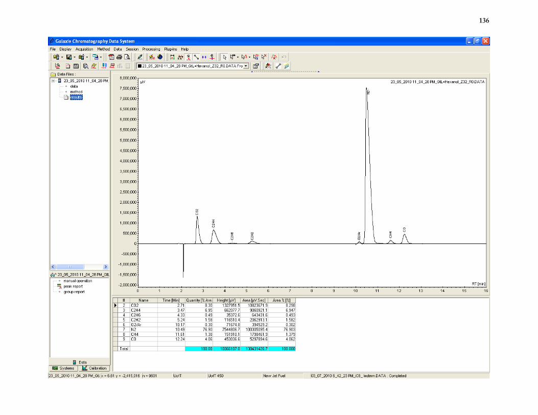
136

Appendix D

Governing Equations for Laminar Diffusion

Flame

137

Mass Conservation

Total mass is conserved in this system. Therefore, the difference between mass in and out of the

control volume is the rate at which mass accumulates within the control volume; i.e., general

form of conservation of mass can be expressed as,

∂ρ∂t + ∇. �ρv�� = 0 �D. 1�

or can be expanded as,

∂ρ∂t + 1

r∂�ρrv��

∂r + 1r

∂�ρv��∂θ + ∂�ρv��

∂z =0 �D. 2� where ρ, t and v are the fluid density, time and velocity. Since the system is at steady state and

there is no variation of speed in θ direction (v� = 0), the equation above can be simplified to,

1r

∂�v�r�∂r + ∂v�∂z =0 (D.3)

Conservation of Momentum

The conservation of momentum can be expressed in both axial and radial direction. The

derivation of simplified axial momentum equation is shown below.

ρ �∂v�∂t + v�∂v�∂r + v�r

∂v�∂θ + v�∂v�∂z � = − ∂P

∂z + ρg� + μ �1r

∂∂r �r ∂v�∂r � + 1

r�∂�v�∂θ� + ∂�v�∂z� �D. 4�

Assuming steady state (""# = 0), no pressure drop (∂P + $%&

� = 0), no variation in θ direction, and neglecting second derivative of v� with respect to z (small based on dimensional analysis),

equation above yields simplified form of the axial momentum equation,

v�∂v�∂z + v�

∂v�∂r = ν 1r

∂∂r �r ∂v�∂r � �D. 5�

138

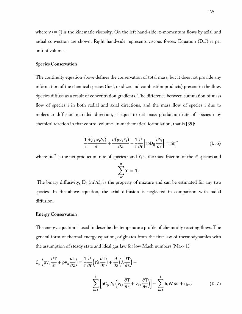
where ν (= μ$) is the kinematic viscosity. On the left hand-side, z-momentum flows by axial and

radial convection are shown. Right hand-side represents viscous forces. Equation (D.5) is per

unit of volume.

Species Conservation

The continuity equation above defines the conservation of total mass, but it does not provide any

information of the chemical species (fuel, oxidizer and combustion products) present in the flow.

Species diffuse as a result of concentration gradients. The difference between summation of mass

flow of species i in both radial and axial directions, and the mass flow of species i due to

molecular diffusion in radial direction, is equal to net mass production rate of species i by

chemical reaction in that control volume. In mathematical formulation, that is [39]:

1r

∂�rρv�Y*�∂r + ∂�ρv�Y*�∂z − 1r

∂∂r +rρD*,

∂Y*∂r - = m/ *000 �D. 6� where m/ *000 is the net production rate of species i and Yi is the mass fraction of the ith species and

2 Y* = 1.3

*45

The binary diffusivity, Dij (m2/s), is the property of mixture and can be estimated for any two

species. In the above equation, the axial diffusion is neglected in comparison with radial

diffusion.

Energy Conservation

The energy equation is used to describe the temperature profile of chemically reacting flows. The

general form of thermal energy equation, originates from the first law of thermodynamics with

the assumption of steady state and ideal gas law for low Mach numbers (Ma<<1).

C7 �ρv�∂T∂r + ρv�

∂T∂z� = 1

r∂∂r �rλ ∂T

∂r� + ∂∂z �λ ∂T

∂z� −

2 +ρC7,*Y* �v*,�∂T∂r + v*,�

∂T∂z�-

*

*45− 2 h*W*ω/ *

*

*45+ q�?@ �D. 7�

139

where CP is the constant pressure heat capacity, λ is thermal conductivity. The h*, W* and ω/ * are the enthalpy of formation, molecular weight and net molar production rate of the ith species,

respectively. The left hand-side of the equation above indicates the thermal energy convection by

the temperature gradient in the element. The first two terms on right hand-side of equation

represents the contribution of thermal heat conduction based on Fourier’s law. The third term,

which includes, vB*, the diffusion velocity of the ith species (in r- and z-directions), shows the contribution of thermal diffusivity on thermal energy. The term, ∑ h*W*ω/ ***45 , is the heat

released from all chemical reactions in which the ith species participated. The last term is

associated to the radiation heat transfer from the element.

140

Appendix E

Sample Hand Calculations

141

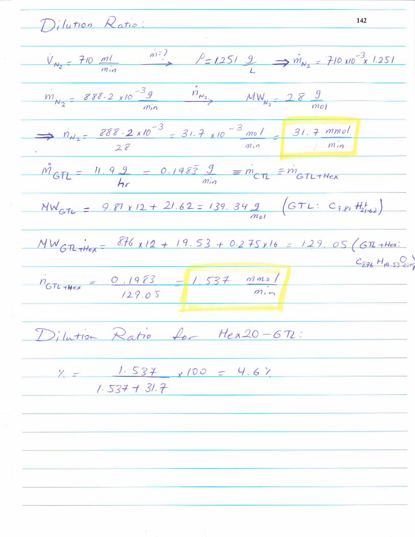
142