Gas Does Affect Oil:

Evidence from Intraday Prices and Inventory Announcements

(JOB MARKET PAPER)

Marketa W. Halova

January 19, 2012

Abstract

Do events in the natural gas market cause repercussions in the crude oil market? Inlight of the enormous impact that price movements in the two largest U.S. energy mar-kets have on the economy, it is important to understand not just the individual marketsbut also how they relate to one another. On this front, the literature presents a puzzle:while economic theory suggests that the oil and gas markets are interlinked through abi-directional causal relationship, empirical research has concluded that the oil marketaffects the gas market but not vice versa. This paper improves on the previous studiesin two ways: by using high-frequency, intraday oil and gas futures prices and by ana-lyzing the effect of specific news announcements from the weekly oil and gas inventoryreports. The results dispel the notion of one-way causality and provide support for thetheory. The reaction of the futures volatility and returns is asymmetric, although thisasymmetry does not follow the “good news” vs. “bad news” pattern from stock and bondmarkets; the response depends on whether the shock is driven by oil or gas inventorygluts or shortages. The two-way causality holds not only for the nearby futures contractbut also for contracts of longer maturities. These findings underscore the importanceof analyzing financial markets in a multi-market context.

Acknowledgements: The author thanks Christopher Baum, Fabio Ghironi, Georg Strasser, Donald Cox,Eyal Dvir, Arthur Lewbel and Ronnie Sadka for their very helpful comments, and the Boston College Library,especially Barbara Mento, for assistance in obtaining the data.Author contact information: Boston College, Department of Economics, Maloney Hall, 21 CampanellaWay, Chestnut Hill, MA 02467; E-mail: halova@bc.edu

1

1 Introduction

This paper studies the relationship between crude oil (referred to as “oil”) and natural gas

(referred to as “gas”). It investigates whether there is two-way causality as suggested by

economic theory or one-way causality as evidenced by previous empirical studies.

Price movements in markets for these two largest U.S. energy sources exert an enormous

influence on the economy.1 For example, Elder and Serletis (2010) show that oil price

volatility has a negative effect on investment, durables consumption and aggregate output,

and exacerbates the response of the economy to a negative oil price shock while dampening

the response to a positive oil price shock. In addition, trading in the oil and gas futures

markets has increased as shown by Figure 1, ranking the oil and gas futures as the first

and the second largest energy futures, and the first and the ninth largest commodity futures

by volume in 2008, respectively.2 In light of this enormous impact of oil and gas on the

macroeconomy as well as the financial markets, it is important to understand not just the

markets for the individual commodities but also how they relate to one another.

Figure 1: Number of futures trades by month

Notes: This figure shows the number of nearby futures trades executed on NYMEX by month.Source: Tick Data, Inc.

On this front, the literature presents a puzzle. Economic theory suggests the existence

of two-way causality between oil and gas markets for several reasons.3 From the demand

1In 2009, oil and gas accounted for 37% and 25% of the energy use in the U.S. See the EIA Annual EnergyReview 2009, Table 1.3.

2Futures Industry Magazine Annual Volume Survey: 2008 A Wild Ride.3Villar and Joutz (2006) provide a summary of the economic theory.

2

perspective, oil and gas are substitutes because a portion of both the power generation and

industrial sectors has the ability to switch between gas and products refined from crude oil

as the production input. Therefore, an increasing oil price resulting from rising demand

will increase the price of gas as some firms in these sectors switch from oil to gas. The

relative price of oil and gas also influences decisions to build new facilities designed to

consume a certain type of fuel. From the supply perspective, an increasing oil price resulting

from increasing demand may lead to increased drilling and production of gas to substitute

away from the more expensive oil, causing an increase in gas supply with a subsequent

decrease in gas price. The gas price may also fall because gas is frequently found in the same

underground reservoirs as oil, so an increasing oil demand satisfied by a higher production

of oil may result in a higher production of gas, reducing the gas price. At the same time,

however, the increasing oil price may intensify competition for resources, such as drilling rigs,

production facilities, and engineering and operations staff used in exploration and production

of both oil and gas, causing an increase in the gas price. In addition, the linkages between oil

and gas prices should have strengthened because of the development of liquified natural gas

technology (LNG), which allows the transportation of gas throughout the world and creates

a world market for gas, a process that has accelerated since the 1990s.

However, the empirical research reviewed in Section 2 has concluded that the causality

runs only in one direction: the oil market affects the gas market but not vice versa. Two

explanations are usually stated. First, the oil market is larger than the gas market. Second,

the oil market is global with prices determined by world supply and demand whereas the gas

market is local with prices determined by local supply and demand. The first explanation

does not seem satisfying since gas is almost as important an energy source as oil for the U.S.

The second explanation also does not seem to hold because oil and gas are partial substitutes

in the power generation and industrial sectors and the LNG technology has connected the

local gas markets.

Since the conflict between theoretical and empirical research represents a puzzle with

unsatisfying explanations, this paper investigates the contradiction. It improves on the

previous studies in two ways. First, it uses high-frequency, intraday New York Mercantile

Exchange (NYMEX) oil and gas futures prices, in contrast to observations taken at a lower

3

frequency, such as the daily, weekly or monthly data used by the previous papers, that do

not capture price interdependencies accurately. Second, it analyzes the effect of specific

news announcements from the weekly oil and gas inventory reports published by the Energy

Information Administration (EIA) of the U.S. Department of Energy instead of conducting

a general analysis of the relationship between the oil and gas prices using, for example,

Granger causality tests as the previous studies. Even though these inventory reports are the

most watched weekly indicators in the oil and gas markets, their effects have not been fully

analyzed.4

Three results follow from this analysis. First, the notion of one-way causality is dispelled,

providing support for the bi-directional causality indicated by the theory for the first time.

Gas inventory announcements affect oil futures volatility and return, and oil inventory an-

nouncements affect gas futures volatility and return. These cross-commodity effects turn out

to be substantial. The effect of gas inventory announcements on oil price volatility is more

than twice as strong as the effect of oil inventory announcements on gas price volatility,

highlighting the importance of spillovers from the gas market to the oil market.

Second, the model allows for different reactions of price volatility and return to inventory

gluts and shortages.5 However, in contrast to the “good news” vs. “bad news” pattern found

in stock and bond markets, the response differs by commodity and type of the shock. A

glut has a larger impact than a shortage for the effect of oil inventory announcements on

oil price volatility. In contrast, a glut has a slightly smaller impact than a shortage for the

effect of gas inventory announcements on oil price volatility, which is also the case for the

effect of gas inventory announcements on gas price volatility. Finally, a glut has the same

effect as a shortage for the effect of oil inventory announcements on gas price volatility. This

highlights the importance of analyzing the data in detail since a general analysis is unable

to uncover these differences.

Third, in contrast to previous studies that analyzed only the nearby futures contract

for the following month, this paper includes contracts with all maturities to investigate how

4For example, the Financial Times noted as of September 21, 2011: “The U.S. is the world’s largest oilconsumer and its weekly petroleum status reports are closely watched.”

5Except for Gregoire and Boucher (2008), who analyze the effect of gas inventory announcements ongas price using daily data, previous papers have not analyzed the asymmetry between inventory gluts andshortages.

4

current news announcements affect financial instruments at various points in the future. The

two-way causality indicated by the cross-commodity effect holds not only for the nearby con-

tract but also for the following seven months’ contracts. The asymmetry effect also persists

across these maturities. The results described above are, therefore, robust to the maturity

structure. In general, the coefficients decrease as the length of the contract increases, sup-

porting the Samuelson (1965) theorem that futures contracts become more volatile as their

expiration date approaches.

In addition to our validating the economic theories on the two largest U.S. energy markets,

identifying precise linkages between these markets is important for several other reasons.

Numerous studies have highlighted the importance of volatility spillovers between the oil

market and financial markets, e.g., stock markets and exchange rate markets, a topic of

interest to regulators and policy-makers.6 To fully understand these spillovers, it is important

to realize that the oil volatility partially originates in another energy market, i.e., the gas

market.

Also, as documented by Buyuksahin, Haigh, Harris, Overdahl and Robe (2008) and

Basu and Gavin (2011), the recent dramatic rise in oil and gas futures trading evidenced

by Figure 1 is mainly due to an increasing number of financial institutions participating in

commodity derivatives such as oil and gas futures. According to Buyuksahin et al (2008),

the share of traditional commercial traders, such as oil and gas exploration, production, and

refining companies who use the futures for commercial hedging decreased from 83% in 2000

to 55% in 2008. At the same time, according to Basu and Gavin (2011), non-commercial

financial traders, such as investment banks, mutual funds, pension funds, university endow-

ment funds and hedge funds, increased their investments in commodity derivatives, in an

attempt to diversify their stock market risk and chase higher yield, higher risk investments.

Since financial institutions played a key role in the recent economic crisis by investing in

complex financial products such as derivatives, and had to be bailed out by the taxpayers,

it is imperative to understand the markets in which they have an increasing exposure.7

6See, for example, Kilian and Park (2009), Cifarelli and Paladino (2010), and Hammoudeh, Yuan andMcAleer (2010).

7Trading in oil and gas options based on oil and gas futures has also been on the rise, with financialinstitutions again becoming more dominant market players. Since the correct pricing of options relies onthe ability to reliably estimate volatility of the underlying asset, i.e., that of the futures contract, it is again

5

Finally, this paper contributes to the discussion of whether oil prices are exogenous or

endogenous to the macroeconomy. While earlier papers, e.g., Hamilton (1985), attribute

oil price changes to exogenous events, such as political instability producing disruptions

in oil supply, more recent studies, e.g., Barsky and Kilian (2002, 2004) and Kilian (2009),

have challenged this view by showing that oil price changes can endogenously follow from

demand changes.8 This paper provides another piece of evidence that oil prices evolve in a bi-

directional causal relationship instead of being exogenous. This improved understanding of

the linkages between the oil and gas markets may provide insight into modeling dependencies

of the macroeconomy on the energy markets. Krichene (2007) develops a model for analyzing

the oil and gas markets with a role for monetary policy. However, in his simultaneous

equations, the gas demand and supply are affected by oil but the oil demand and supply

are not affected by gas. Such a misspecification may lead to misguided policies. These

considerations underscore the importance of analyzing energy (and financial) markets in a

multi-market context.

2 Literature Review

Although theory suggests a two-way relationship between the oil and gas markets, the empir-

ical research by Pindyck (2004), Villar and Joutz (2006), Asche, Osmundsen and Sandsmark

(2007), Brown and Yucel (2007) building on an earlier paper by Brown (2005), and Hartley,

Medlock and Rosthal (2008) concluded that the causality runs only in one direction: the oil

market affects the gas market but not vice versa.9 Onour (2009) also noted that the gas

price is affected by the oil price, especially at low oil prices (below $40 per barrel), but did

not investigate the sensitivity of oil to gas. See Table 9 in Appendix A for an overview of

critical to understand how the volatility is partially driven by spillovers from another market.8Hamilton (2008) and Kilian (2008) provide literature reviews of the relationship between oil prices and

the macroeconomy.9Pindyck (2004) conducted Granger causality tests using the conditional volatility from GARCH models.

When estimating the GARCH model with daily data, he concluded that the oil market affected the gasmarket but not the other way around which he said was the expected result. When estimating the GARCHmodel with weekly data, he obtained the opposite result but disregarded it, arguing that correlations betweenthe oil and gas volatilities are low in the weekly model.

6

the data used in these papers.10

While the above papers claim that the gas market does not affect the oil market, this

study uncovers evidence of such a relationship. It differs from the previous empirical papers

in two respects. First, it takes advantage of NYMEX intraday oil and gas futures prices, i.e.,

prices at a higher frequency than the daily, weekly or monthly prices used by the previous

papers. Second, in contrast to the previous papers that conduct a general analysis of the

relationship between the oil and gas prices using, for example, Granger causality tests, this

paper analyzes the effect of specific news announcements: the weekly oil and gas inventory

reports published by the EIA.

Four papers have analyzed the effect of inventory announcements on intraday energy

prices. Linn and Zhu (2004) studied the effect of gas inventory announcements on intraday

gas futures price return and volatility from 1999 through 2002 and concluded that volatility

increased after inventory announcements. However, they included only the actual inventory

level. This is an issue because the efficient market theory states that only the unanticipated

component of news announcements matters because the anticipated component has been

built into price forecasts by rational economic agents. Therefore, the correct methodology

for analyzing the impact of news announcements on prices requires that market expectations

be subtracted from the actual value to arrive at the unanticipated component.

Gay, Simkins and Turac (2009) investigated whether investors learned about analyst

accuracy using gas inventory announcements and gas futures prices from 1997 through 2005.

Focusing only on futures return and disregarding price volatility, they concluded that the oil

futures return reacted to analyst forecasts.

10Several other papers have studied the relationship between oil and gas markets without analyzing causal-ity. Yucel and Guo (1994) showed that oil, gas and coal prices were cointegrated from 1974 through 1990although only oil and coal prices were cointegrated from 1947 through 1974. Panagiotidis and Rutledge(2007) also found a cointegrating relationship between oil and gas prices, while Serletis and Rangel-Ruiz(2004) reported that the oil and gas relationship had weakened and Bachmeier and Griffin (2006) concludedthat the oil, gas and coal markets were only very weakly integrated. Wang, Wu and Yang (2008) showedthat the correlation between oil and gas prices did not exhibit long-memory, implying a weak relationshipin the long run. Marzo and Zagaglia (2008) noted that the correlation between the oil and gas prices hasbeen rising since 2000 although this correlation was low on average over two thirds of the sample period.See Table 10 in Appendix A for an overview of the data used in these papers. Also, related papers studiedrelationships between other commodities. Serletis and Herbert (1999) focused on daily gas, fuel oil, andpower prices from 1996 through 1997, while Ohana (2010) analyzed daily spot gas and heating oil futuresprices from 2000 through 2009.

7

Bjursell, Gentle and Wang (2009) considered, among other things, the effect of oil inven-

tory announcements on oil intraday volatility and the effect of gas inventory announcements

on gas intraday volatility. Instead of subtracting the market expectations from the actual

values to arrive at the unexpected component, they estimated the “surprise” based on his-

torical inventory levels. They concluded that this ”surprise” increased volatility in gas and

heating oil prices.

Chang, Daouk and Wang (2009) investigated whether investors learn about analyst ac-

curacy using oil inventory announcements and oil futures prices from 2003 through 2005.

Focusing only on price return and disregarding price volatility, they concluded that the oil

price return rises (falls) when analysts forecast a decrease (increase) in supplies.11

None of these four papers on the effect of inventory announcements focused on the cross-

commodity effect, i.e., the effect of gas inventory announcements on the oil price and the

effect of oil inventory announcements on the gas price. Also, these papers did not distinguish

between positive and negative surprises, which prevented them from discussing asymmetries

between effects of inventory shortages and gluts. Finally, they focused only on the nearby

futures contract, ignoring the effect on contracts with longer maturities.12

11Three of the above papers on the causal relationships between the oil and gas markets allowed inventoryto play a limited role. Villar and Joutz (2006), Brown and Yucel (2007), and Hartley, Medlock and Rosthal(2008) included the gas inventory but ignored the oil inventory. More importantly, they included only theactual inventory, i.e., they failed to subtract market expectations of the inventory.

12Seven papers have analyzed the effect of other news announcements on oil prices. Ghura (1990) focusedon the impact of five U.S. macroeconomic announcements, exchange rates and interest rates on price returnsof oil and nineteen other commodities using daily prices from 1985 through 1989. Kilian and Vega (2008)conducted a more comprehensive study by analyzing the impact of thirty U.S. macroeconomic announcementson price returns of oil and gasoline using daily data from 1983 through 2008. Roache and Rossi (2009)analyzed the impact of thirteen U.S. and European announcements on price returns and volatilities of oiland eleven other commodities using daily data from 1997 through 2009. Guidi, Russell and Tarbert (2006),Schmidbauer and Rosch (2009), and Lin and Tamvakis (2010) studied the effect of OPEC decisions whileLeinert (2010) considered the effect of unanticipated discoveries of giant oil fields. Three papers analyzed theeffect of other announcements on gas prices: Ates and Wang (2007), Mu (2007), and Gregoire and Boucher(2008).

8

3 Data

3.1 Oil and Gas Futures Prices

Oil and gas futures contracts are traded on two main exchanges: the NYMEX in Chicago

and the InterContinental Exchange (ICE) in London. This paper focuses on the NYMEX

futures data because NYMEX is more liquid than ICE.13 This proprietary data is provided

by Tick Data, Inc., a company that specializes in intraday time series data for equities,

futures and options.14 The data are transaction data, i.e., not bid-ask quotes.

Light Sweet Crude Oil futures started trading on NYMEX under the symbol CL on

March 30, 1987. Currently, the trading day takes place on Mondays through Fridays from

9:00 a.m. till 2:30 p.m. Eastern Time.15 The standardized contract is for 1,000 barrels

with the price quoted in U.S. dollars per barrel. Futures contracts with different maturities

are available. The shortest maturity, called the nearby contract, is for the following month.

The longest maturity is nine years. Trading ceases on the third business day prior to the

twenty-fifth calendar day of the month preceding the delivery. At expiration, oil has to be

physically delivered to Cushing, OK.16 Figure 2 presents the oil nearby contract price from

2003 to 2010.

Natural gas futures started trading on NYMEX under the symbol NG on January 4,

1993. The trading hours are identical to those for oil. The standardized contract is for

10,000 million British thermal units (mmBTU) with the price quoted in U.S. dollars per

mmBTU. Maturities from one month to twelve years are available. Trading ceases three

business days prior to the first day of the delivery month. At expiration, gas has to be

physically delivered to Henry Hub, LA. Figure 3 presents the gas nearby contract price from

2003 to 2010.

Very few market participants choose to make physical delivery at contract expiration.

Instead, they roll over their positions into a new contract. Two methodologies are used in this

paper to create a continuous record of the futures contract prices. In the first methodology,

13See Downey (2009) for description of the oil market.14See www.tickdata.com.15Until January 31, 2007, the trading day started at 10:00 a.m. Night trading is not analyzed in this paper

since the day and night trading sessions may differ from the information arrival standpoint.16See website of CME Group that owns NYMEX: www.cmegroup.com.

9

Figure 2: Crude oil futures price

Notes: This figure shows the price of the NYMEX crude oil nearby futures contract per barrel in U.S. dollars.Source: Tick Data, Inc.

Figure 3: Natural gas futures price

Notes: This figure shows the price of the NYMEX natural gas nearby futures contract per million British thermal units in U.S. dollars.Source: Tick Data, Inc.

the current contract is used until the expiration date. However, as market participants begin

rolling over their positions on the preceding days, trading may be thin during the last days

before the contract expiration date, causing unusual price movements. Therefore, the second

10

methodology switches to the next contract as soon as its daily contract volume exceeds the

current contract volume. The results do not materially differ between the two methods.

Therefore, only results using the expiration date method are reported.17

3.2 Weekly Petroleum Status Report

The data on the U.S. oil inventory come from the Weekly Petroleum Status Report published

by the EIA. This report is prepared by the EIA based on companies submitting weekly forms

stating their current oil inventory, as mandated by law.18 The first report was published on

August 20, 1982. The report is released weekly on Wednesday at 10:30 am for the week

ending on the previous Friday. If Monday, Tuesday or Wednesday fall on a public holiday,

the report is released on the following Thursday at 11:00 am.19 See Appendix B for a

discussion of the adjustment to holidays. Only commercial inventory is considered in this

paper, i.e., the Strategic Petroleum Reserves held by the U.S. government are excluded. The

data are in thousands of barrels.

3.3 Weekly Natural Gas Storage Report

The data on the gas inventory in the the U.S. Lower 48 states come from the Weekly Natural

Gas Report published by the EIA based on companies submitting weekly forms stating their

current gas inventory, as mandated by law.20 The first report was published on December

31, 1993. The report is released weekly on Thursday at 10:30 am for the week ending on

the previous Friday unless Thursday falls on a public holiday. There are twelve such holiday

weeks in the sample period. It is assumed that the report was released at 10:30 am on

the following Friday during these holiday weeks.21 See Appendix B for a discussion of the

17Another method chooses a particular date, e.g., the 15th calendar day of each month to switch from thenearby contract to the second nearby contract in an attempt to model the market participants’ behavior.This approach is not used in this paper because it is arbitrary.

18See www.eia.doe.gov.19These holiday weeks are skewing the intraday pattern graphs in Sections 5.1.1 and 5.2.1. The regressions

are correct because the data show the inventory reports on the days and intervals when they are actuallyreleased. As a robustness check, however, these weeks are eliminated from the data. The results do notchange materially. The results reported in this paper include the holiday weeks.

20See www.eia.doe.gov.21The American Gas Association (AGA) published this report prior to the end of April of 2002. The

AGA released the report on Wednesdays after NYMEX market closing time from December 31, 1993 until

11

adjustment to holidays. The data are in billions of cubic feet.

3.4 Expectations of the Weekly Petroleum Status Report

Bloomberg conducts a weekly survey of approximately twenty industry experts asking them

what they expect the oil inventory excluding the Strategic Petroleum Reserves to be once

released by the EIA, and publishes the minimum, maximum, mean and median values of

the expert forecasts (in thousands of barrels). This paper uses the median forecast.22 The

survey is published on Monday or Tuesday, i.e., prior to the actual values being released by

the EIA. The first survey was conducted on June 13, 2003.23 As explained in Section 4, the

“surprise” is calculated as the difference between the EIA inventory announcement and the

Bloomberg survey forecast.

3.5 Expectations of the Weekly Natural Gas Storage Report

Bloomberg conducts a weekly survey of approximately twenty-five industry experts asking

them what they expect the gas inventory to be once released by the EIA (in billions of cubic

feet), using the same methodology as for oil. The first survey was conducted on May 3, 2002.

4 Methodology

Deciding on the length of the intraday time interval involves choosing between noise due

to the data microstructure and loss of information. Using the volatility signature plot that

shows the scaled realized volatility, i.e., daily average of squared returns, against time in-

tervals in multiples of one minute as outlined by Andersen, Bollerslev, Diebold and Labys

(2000), the 10-minute interval is chosen as the appropriate length. See Appendix C for

February 25, 2000 and between 2:00 pm and 2:15 pm from March 3, 2000 until April 26, 2002. The EIA tookover on May 3, 2002. However, as this study is limited to the period from June 13, 2003 until September24, 2010, it is not affected by the change of the release day from Wednesday to Thursday.

22The data can be found on the Bloomberg terminal under the code ECO with “North America” underRegion, “U.S.” under Country, and “10) Energy/Commodities” under Type. The list of economists surveyed,including the date of the survey, can be obtained by typing in “12”.

23Note that Bloomberg asks the experts by how much they expect the inventory to change compared withthe previous week. Therefore, to arrive at the expected inventory, it is necessary to add the previous week’sactual inventory and the experts’ expectation of the change in inventory.

12

volatility signature plots for oil and gas prices.24 For example, the first 10-minute interval

contains trades from 9:00:00 till 9:09:59.25 There are 27 and 33 intervals within a trading day

depending on whether the market opens at 10 a.m. or 9 a.m. The days when the NYMEX

market closes earlier, usually due to an upcoming holiday, are eliminated to prevent skewing

intraday patterns.26 Missing prices are set equal to the previous prices.27 The resulting

sample period contains 54,884 10-minute intervals on 1,826 days from June 13, 2003 until

September 24, 2010, a period of 380 weeks.

Let Pj be the price at the end of 10-minute interval j. Since both oil and gas price series

are non-stationary, the return, i.e., the difference between the log price at the end of interval

j and the log price at the end of interval j-1, Rj ≡ ln(Pj)− ln(Pj−1), is used. The resulting

return series is stationary as gauged by an augmented Dickey-Fuller test.

This paper analyzes the effect of announcements on price returns as well as volatility,

defined as the absolute value of the returns, |Rj|, following, for example, Ding, Granger and

Engle (1993), Ederington and Lee (1993), Gwilym, McMillan and Speight (1999), McKenzie

(1999), Bollerslev, Cai and Song (2000), and Ederington and Guan (2005). See Figures 4

and 5 for oil and gas absolute price returns, respectively.

The methodology for analyzing the effect of news announcements on prices assumes

efficient markets, implying that only the unanticipated component of news announcements

matters because the anticipated component has been built into market participants’ price

forecasts. The unexpected component is the difference between the actual value, Akj, and

the expected value, Ekj, where k ∈ {O,G} stands for oil and gas announcements. Since this

difference is in thousands of barrels and billions of cubic feet for oil and gas, respectively,

it is divided by the actual value and then multiplied by 100. The resulting “surprise”,

Skj ≡ Akj−Ekj

Akj× 100, can then be interpreted as a percentage deviation of the expectations

from the actual values.28 Statistics for the oil inventory surprise, SO, and the gas inventory

24See Dacorogna, Gencay, Muller, Olsen and Pictet (2001) for a discussion of scaling factors. Also, notethat the realized volatility is used only to choose the appropriate interval. It is not used in the regressions.The dependent variable in the volatility regressions is defined as the absolute return.

25As a robustness check, the analysis is repeated using 15-minute and 30-minute intervals. The results donot change materially.

26There are only 20 such days within the sample period.27There are very few such missing observations (0.20% and 0.45% of all observations for the oil and gas

nearby contracts, respectively).28Balduzzi, Elton and Green (2001) implement another methodology for standardizing announcement

13

Figure 4: Crude oil futures price volatility

Notes: This figure shows the price volatility of the NYMEX crude oil nearby futures contract defined as absolute return.Source: Tick Data, Inc.

Figure 5: Natural gas futures price volatility

Notes: This figure shows the price volatility of the NYMEX natural gas nearby futures contract defined as absolute return.Source: Tick Data, Inc.

surprise, SG, are summarized in Table 1. Since the mean values of these variables are

units. They divide the difference between the actual and expected values by its sample standard deviationσk and interpret the coefficient as the change in oil price return for one standard deviation change in thesurprise. In this paper, dividing by the actual value is preferred to allow for interpreting the surprise as apercentage deviation of the expectation from the actual value.

14

close to zero, the Bloomberg survey can be considered unbiased, i.e., the analysts do not

systematically overforecast or underforecast.

Table 1: Summary statistics for oil and gas inventory surprise variables

Min Max Mean Standard DeviationOil inventory surprise, SO -2.85% 2.82% -.02% .94%

Gas inventory surprise, SG -1.55% 2.93% .05% .46%

A positive surprise, Skj > 0, i.e., Akj > Ekj, means that the actual inventory, when

announced by the EIA, is higher than what the analysts expected. In other words, the ana-

lysts underforecast the actual inventory resulting in an inventory glut. A negative surprise,

Skj < 0, i.e., Akj < Ekj, means that the actual inventory, when announced by the EIA, is

lower than what the analysts expected. In other words, the analysts overforecast the actual

inventory, resulting in an inventory shortage.

To allow for the possibility of asymmetric reaction of the price return and volatility to

shortages and gluts, indicators, I(Skj > 0), are created for oil and gas that take on value

of 1 if Skj > 0 and 0 otherwise. These indicators are then multiplied by the surprise, i.e.,

Skj × I(Skj > 0). This allows interpreting the coefficient on the surprise, Skj, as the effect of

a shortage. The sum of the coefficients on Skj and Skj × I(Skj > 0) can then be interpreted

as the effect of a glut.

The effect of the announcements is analyzed using ordinary least squares (OLS) regres-

sion. Several control variables are included in the regressions in addition to the above surprise

variables. As suggested by Andersen, Bollerslev, Diebold and Vega (2003), lags of surprise

and dependent variable are added to allow for autocorrelation.29

A beginning-of-day dummy is included to account for unusual price movements at the

beginning of the day and to account for the change in the beginning of the trading day

from 10:00 to 9:00 on February 1, 2007. This dummy takes on the value of 1 during the first

interval of the day and 0 in all other intervals. An end-of-day dummy is included in the same

2933 lags are used since a trading day includes 33 10-minute intervals. In an alternative specification, themodel is modified to include lagged cross-commodity terms, i.e., the oil price volatility (return) equationsinclude gas price volatility (return) lags. The results do not change.

15

way to account for unusual price movements at the end of the day. These time-of-the-day

effects have been identified in many financial markets, for example by Becker, Finnerty and

Kopecky (1993), Gwilym, McMillan and Speight (1999), Bollerslev, Cai and Song (2000),

and Linn and Zhu (2004).30 A first-trading-day dummy is included that takes on the value

of 1 in all intervals on the day after a non-trading day, i.e., after a weekend or a holiday, to

allow for effects due to the market being closed for an extended period of time. A trader

composition variable, defined as the ratio of non-commercial financial traders volume to the

traditional commercial traders volume, is added to account for a change in the composition

of firms trading oil futures, as documented by Buyuksahin et al (2008). These authors

show that the proportion of non-commercial financial traders has been on the rise and the

proportion of traditional commercial traders has declined. The three-month Treasury bill

rate is included because Pindyck (2004) shows that this interest rate helps explain the oil

return because it affects the cost of holding inventory.

Trading volume is added to account for various unobservable sources of volatility. One

unit of volume represents 1,000 executed contracts. Disagreement exists on whether con-

temporaneous or lagged volume should be used. Foster (1995) concluded that oil volatility

and volume are contemporaneously correlated and driven by the same factors, assumed to

be information. He showed that lagged volume explains current volatility which means that

lagged volume rather than contemporaneous volume should be used as a control variable

to avoid endogeneity issues. Kocagil and Shachmurove (1998) corroborated this by provid-

ing evidence of two-way Granger causality between oil volatility and volume. Fujihara and

Mougoue (1997) argued that volume is a significant explanatory variable for oil volatility

even though factors other than volume affect the persistence of volatility. In contrast, Gi-

rard, Sinha and Biswas (2008) concluded that volume not only leads oil and gas volatility

but is exogenous to it, which implies that it can be used for forecasting volatility and as a

proxy for the flow of information, suggesting contemporaneous volume can be included in

the regressions. For gas, Herbert (1995) concluded that lagged volume influences current

price volatility but lagged price volatility has much less of an influence on current volume.

30Alternative specifications are run where the beginning-of-day (end-of-day) dummy took on the value of1 for the first (last) two and three intervals. The results do not change.

16

Since the previous papers disagree on whether contemporaneous or lagged volume should be

used as a control variable in the volatility regression, both specifications are implemented.

The results are very similar. The lagged volume specification is reported in this paper.31

Control variables for gasoline inventory, distillate fuel oil (referred to as “distillate”)

inventory and refinery utilization are added because these data are included in the Weekly

Petroleum Storage Report.32 Since these data are released at the same time as the oil

inventory data, their announcements could possibly skew the results. There are no other

weekly announcements made by any U.S. government agency which coincide with the oil

and gas inventory announcements.33

For the futures return, the regression is:

Rj = α+ ΣIi=1βiRj−i + ΣK

k=1ΣLl=0γklSk,j−l + ΣK

k=1ΣLl=0δklSk,j−l × I(Sk,j−l > 0) + ΣM

m=1θm{Zm}+ εj , (1)

where {k} includes oil, gas, gasoline, distillate and refinery utilization, i and l stand for

lags of returns and surprises, respectively, and {Zm} includes dummies for the beginning-of-

day, end-of-day and the first-trading-day, and controls for trader composition, three-month

Treasury bill rate, and lagged volume.

Similarly, for the futures volatility, the regression is:

|Rj | = α+ΣIi=1βi|Rj−i|+ΣK

k=1ΣLl=0γklSk,j−l +ΣK

k=1ΣLl=0δklSk,j−l×I(Sk,j−l > 0)+ΣM

m=1θm{Zm}+εj . (2)

Newey-West standard errors are used to account for heteroskedasticity and autocorrela-

tion in the error term εj.34

31In an alternative method of accounting for various unobservable sources of volatility, the Chicago BoardOptions Exchange Volatility Index (VIX) is included as a measure of the stock market volatility and investorsentiment in general. The results do not change.

32Distillate includes diesel fuels used in on-highway engines, e.g., automobiles and trucks, and off-highwayengines, e.g., railroad locomotives and agricultural machinery, as well as fuel oils used for heating and powergeneration. Refinery utilization is defined as the ratio of gross inputs used in the atmospheric oil distillationunits to the operable capacity of the units. For more detail, see Definitions of Petroleum Products and OtherTerms on www.eia.doe.gov.

33The Weekly Petroleum Storage Report includes other data, e.g., propane inventory and jet fuel inventory.However, Bloomberg does not conduct surveys for these commodities. Therefore, they cannot be includedin the regression. It is unlikely they would have a major effect on the results of this paper.

34Note that the above regressions do not suffer from endogeneity due to a two-way relationship between oilprices and oil inventory because the inventory variable on the right-hand side is not the actual inventory; itis the unanticipated component of the inventory changes. As such, it is not a decision variable of the marketparticipants.

17

Since the oil and gas prices exhibit time-varying volatility depicted in Figures 4 and 5,

generalized autoregressive conditional heteroskedasticity (GARCH) models lend themselves

as tools for analyzing the data in addition to the OLS. Four specifications are presented.

First, the GARCH(1,1) model that includes one ARCH term and one GARCH term with

the Gaussian distribution of errors is used as a benchmark:

Rj = α+ ΣIi=1βiRj−i + ΣK

k=1ΣLl=0γklSk,j−l + ΣK

k=1ΣLl=0δklSk,j−l × I(Sk,j−l > 0) + ΣM

m=1θm{Zm}+ εj , (3)

h2j = ν + φh2

j−1 + ζεj−1, (4)

where equation (3) is the mean equation, equation (4) is the conditional variance equation,

and the distribution of the error conditional on an information set at time j, Ψj, is assumed

to be εj|Ψj ∼ N [0, h2j ].

Second, a GARCH(1,1) model with the t distribution is implemented to account for

the distribution’s heavy tails. Third, a GARCH-in-mean(1,1) model with the Gaussian

distribution that lets the expected value of the return depend on its conditional variance is

used. The mean equation then becomes:

Rj = α+ΣIi=1βiRj−i+ΣK

k=1ΣLl=0γklSk,j−l+ΣK

k=1ΣLl=0δklSk,j−l×I(Sk,j−l > 0)+ΣM

m=1θm{Zm}+ψh2j+εj . (5)

Finally, an EGARCH(1,1) model with the Gaussian distribution that allows for an asym-

metric reaction to positive and negative innovations is implemented with the conditional

variance equation:

log(h2j ) = ν + φ log(h2

j−1) + ω

∣∣∣∣∣ εj−1√hj−1

∣∣∣∣∣+ ρεj−1√hj−1

, (6)

where the term ρ εj−1√hj−1

captures the asymmetry because positive innovations εj > 0 are

allowed to have different effects on the conditional variance than negative innovations εj < 0.

The above regressions are run for the futures nearby contract as well as the contracts of

longer maturities to investigate how current news announcements affect financial instruments

at various points in the future.

18

5 Results

5.1 Oil Price Volatility

5.1.1 Intraday Pattern Graphs

Figure 6 shows the intraday pattern of oil price volatility.35 In panel a), absolute returns for

each 10-minute interval are averaged across all days in the data sample. In addition to a U-

shaped pattern due to the market opening and closing, one feature stands out.36 The 10:40

a.m. interval shows a spike in volatility. Panels b), c) and d) display the intraday pattern

of volatility by day. In panel b), the absolute returns for each interval are averaged only for

Mondays. While the U-shaped pattern is still visible, the 10:40 a.m. spike disappears. The

graphs for Tuesdays and Fridays, not shown in this paper, look similar. Panel c) shows the

intraday volatility pattern for Wednesdays, i.e., the day when the Weekly Petroleum Storage

Report is released at 10:30 a.m. As documented by Bjursell, Gentle and Wang (2009), the

10:40 a.m. spike is due to this oil inventory news announcement. However, panel d) for

Thursdays shows a similar pattern with a smaller magnitude. This paper hypothesizes that

the 10:40 a.m. spike is due to the release of the Weekly Natural Gas Storage Report at 10:30

a.m. This cross-commodity effect, suggesting that the gas market influences the oil market,

has not been observed in previous research.37

5.1.2 Cross-Commodity Effect

Table 2 shows regression results for the price volatility of the oil nearby futures contract.

Specification (1) includes the oil inventory variables as well as control variables that have

been used in other papers to explain the oil price volatility, as described in Section 4.38

35The intraday pattern graphs do not display the first interval to avoid skewing the graphs by the overnightgap as the first interval is affected by not only by the first ten minutes of the trading day but also the periodsince the market closed on the previous day.

36The fact that the data sample includes the period from June 13, 2003 till January 31, 2007 when themarket opened at 10 a.m. as well as the period from February 1, 2007 till September 24, 2010 when themarket opened at 9 a.m. creates a “double-U” because the volatility is higher after 9 a.m. and after 10 a.m.

37The smaller spike on Thursdays in the 11:10 a.m. interval is due to the Weekly Petroleum StorageReport being released on Thursdays at 11:00 a.m. if Monday, Tuesday or Wednesday fall on a holiday, asdiscussed in Section 3.2.

38The first-trading-day dummy, refinery utilization variables, and lags of inventory surprises are not sig-nificant, so the specification reported in this paper excludes them.

19

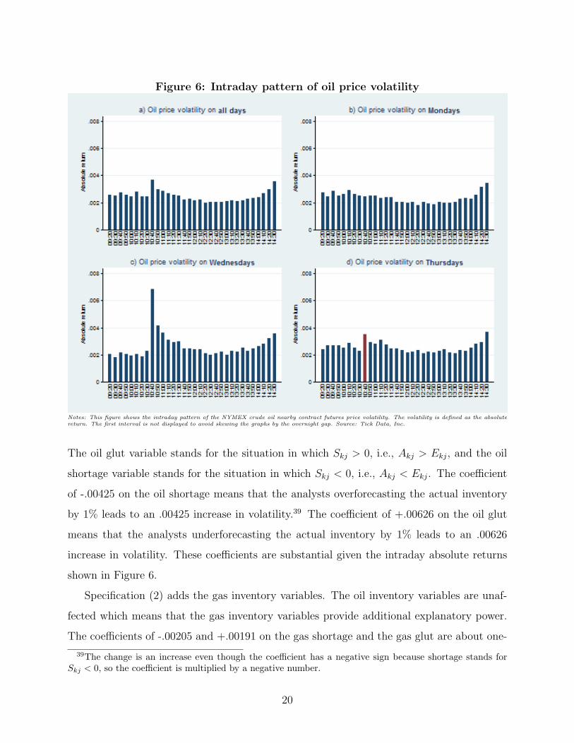
Figure 6: Intraday pattern of oil price volatility

Notes: This figure shows the intraday pattern of the NYMEX crude oil nearby contract futures price volatility. The volatility is defined as the absolutereturn. The first interval is not displayed to avoid skewing the graphs by the overnight gap. Source: Tick Data, Inc.

The oil glut variable stands for the situation in which Skj > 0, i.e., Akj > Ekj, and the oil

shortage variable stands for the situation in which Skj < 0, i.e., Akj < Ekj. The coefficient

of -.00425 on the oil shortage means that the analysts overforecasting the actual inventory

by 1% leads to an .00425 increase in volatility.39 The coefficient of +.00626 on the oil glut

means that the analysts underforecasting the actual inventory by 1% leads to an .00626

increase in volatility. These coefficients are substantial given the intraday absolute returns

shown in Figure 6.

Specification (2) adds the gas inventory variables. The oil inventory variables are unaf-

fected which means that the gas inventory variables provide additional explanatory power.

The coefficients of -.00205 and +.00191 on the gas shortage and the gas glut are about one-

39The change is an increase even though the coefficient has a negative sign because shortage stands forSkj < 0, so the coefficient is multiplied by a negative number.

20

half and one-third the size of their oil counterparts, respectively, indicating the gas inventory

announcements have a sizeable effect on the oil price volatility. This influence of the gas

market on the oil market has not been documented before.

Specification (3) adds control variables for the gasoline and distillate inventory. Even

though adding these variables decreases the oil shortage and oil glut coefficients, the gas

shortage and gas glut coefficients are unaffected, confirming the cross-commodity effect.

In fact, the gas inventory variables become more important relative to the oil inventory

variables. The gas shortage coefficient becomes almost as large as the oil shortage coefficient

and the gas glut coefficient becomes about half the size of the oil glut coefficient. This

cross-commodity effect provides support for the theories on spillovers between the oil and

gas markets described in the Introduction.

5.1.3 Joint Model of Oil and Gas Price Volatility and the Asymmetry Effect

To put the effect of gas inventory announcements on the oil price volatility in perspective, the

effect of oil inventory announcements on the gas price volatility is analyzed for comparison.

Since errors may be correlated across the oil and gas regressions, a seemingly unrelated

regression (SUR) is estimated.40 Table 3 displays the results for the oil and gas inventory

variables. Again, the coefficients are sizeable given the intraday absolute returns shown in

Figure 6.

The effect of both gas gluts and gas shortages on the oil price volatility is more than

twice as strong as the effect of oil gluts and oil shortages on the gas price volatility. This

underscores the cross-commodity effect and highlights the importance of the gas market

spillovers for the oil market.

In addition to the cross-commodity effect, the joint model results in Table 3 offer an

interesting picture of asymmetries. Numerous studies have shown that in stock and bond

markets, an unexpected price decrease, i.e., “bad news”, is associated with a higher volatility

than an unexpected price increase, i.e., “good news” (e.g., Glosten, Jagannathan and Runkle

(1993)). In the oil and gas markets, the evidence is mixed. The finding from the stock and

bond markets was corroborated by Susmel and Thompson (1997) using monthly gas data

40The SUR results do not materially differ from running regressions separately for oil and gas.

21

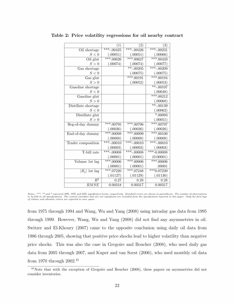
Table 2: Price volatility regressions for oil nearby contract

(1) (2) (3)Oil shortage ***-.00425 ***-.00426 ***-.00231

S < 0 (.00051) (.00051) (.00066)Oil glut ***.00626 ***.00627 ***.00433S > 0 (.00074) (.00074) (.00077)

Gas shortage **-.00205 ***-.00209S < 0 (.00075) (.00075)

Gas glut ***.00191 ***.00194S > 0 (.00052) (.00053)

Gasoline shortage **-.00107S < 0 (.00048)

Gasoline glut ***.00212S > 0 (.00068)

Distillate shortage **-.00139S < 0 (.00062)

Distillate glut *.00093S > 0 (.00051)

Beg-of-day dummy ***.00795 ***.00796 ***.00797(.00026) (.00026) (.00026)

End-of-day dummy ***.00098 ***.00099 ***.00100(.00008) (.00008) (.00008)

Trader composition ***-.00010 ***-.00010 ***-.00010(.00003) (.00003) (.00003)

T-bill rate ***-.00008 ***-.00008 ***-0.00008(.00001) (.00001) (0.00001)

Volume 1st lag ***.00006 ***.00006 ***.00006(.00001) (.00001) .00001

|Rj | 1st lag ***.07220 ***.07248 ***0.07239(.01127) (.01129) (.01130)

R2 0.27 0.28 0.28RMSE 0.00318 0.00317 0.00317

Notes: ***, ** and * represent 99%, 95% and 90% significance levels, respectively. Standard errors are shown in parenthesis. The number of observationsis 54,850 in all specifications. The control variables that are not significant are excluded from the specification reported in this paper. Only the first lagsof volume and absolute return are reported to save space.

from 1975 through 1994 and Wang, Wu and Yang (2008) using intraday gas data from 1995

through 1999. However, Wang, Wu and Yang (2008) did not find any asymmetries in oil.

Switzer and El-Khoury (2007) came to the opposite conclusion using daily oil data from

1986 through 2005, showing that positive price shocks lead to higher volatility than negative

price shocks. This was also the case in Gregoire and Boucher (2008), who used daily gas

data from 2005 through 2007, and Kuper and van Soest (2006), who used monthly oil data

from 1970 through 2002.41

41Note that with the exception of Gregoire and Boucher (2008), these papers on asymmetries did notconsider inventories.

22

Table 3: SUR model for oil and gas price volatility

Oil price volatility Gas price volatilityOil shortage ***-.00232 **-.00089

S < 0 (.00030) (.00042)Oil glut ***.00434 **.00089S > 0 (.00030) (.00043)

Gas shortage ***-.00217 ***-.02432S < 0 (.00061) (.00087)

Gas glut ***.00200 ***.02110S > 0 (.00044) (.00064)

Notes: ***, ** and * represent 99%, 95% and 90% significance levels, respectively. Standard errors are shown in parenthesis. The number ofobservations is 54,850. Only the oil and gas inventory variables are reported to save space.

In our findings, price decreases are associated with inventory gluts and price increases

are associated with inventory shortages in accordance with laws of demand and supply as

shown in Table 6. The relative response of volatility to the price decreases, i.e., inventory

gluts, and price increases, i.e., inventory shortages, differs by commodity. A glut has a larger

impact than a shortage for the effect of oil inventory announcements on oil price volatility.

In contrast, a glut has a slightly smaller impact than a shortage for the effect of gas inventory

announcements on oil price volatility, which is also the case for the effect of gas inventory

announcements on gas price volatility. Finally, a glut has the same effect as a shortage for

the effect of oil inventory announcements on gas price volatility. This shows the asymmetry

depends on the source of the shock and highlights the importance of analyzing the data in

detail since general statements may miss the fine differences.

5.1.4 Effect across Futures Contract Maturities

To investigate how current news announcements affect financial instruments at various points

in the future, the specification (3) is run for the nearby contract, denoted as Contract 1 and

the following seven months’ contracts for oil and gas. Since errors may be correlated across

the regressions for the different maturities, SUR is applied.42

42This leads to the slight differences between results for the nearby contract reported in Table 2 that usesOLS and Table 4 that uses SUR. Also, since contracts with longer maturities are traded less frequently, thesecontracts have more missing observations than the nearby contract. Oil contracts 2 through 8 have 0.42%,6.79%, 25.69%, 46.43%, 60.76%, 71.30% and 77.54% missing observations, respectively. Gas contracts 2through 8 have 1.19%, 5.83%, 11.83%, 17.97%, 24.81%, 33.24% and 40.07% missing observations, respectively.As in the nearby contract, the missing observations are set equal to the previous observation. However, since

23

Table 4 displays the results for the oil and gas inventory variables. See Appendix D for

the other regressors. The two-way causality indicated by the cross-commodity effect holds

across the maturity structure as the oil and gas inventory variables remain significant for

the longer maturities. The asymmetry effect also persists across the maturities. The results

described above are, therefore, robust to the maturity structure. In general, the coefficients

decrease as the length of the contract increases, supporting the Samuelson (1965) theorem,

which states that futures contracts become more volatile as their expiration date approaches.

Table 4: Price volatility of contracts with longer maturities

Panel a): Oil contractsContract 1 Contract 2 Contract 3 Contract 4 Contract 5 Contract 6 Contract 7 Contract 8

Oil shortage ***-.00223 ***-.00197 ***-.00185 **-.00067 ***-.00124 *-.00057 -.00005 -.00048S < 0 (.00030) (.00026) (.00026) (.00028) (.00030) (.00031) (.00031) (.00031)

Oil glut ***.00428 ***.00352 ***.00334 ***.00208 ***.00224 ***.00083 ***.00116 .00043S > 0 (.00031) (.00027) (.00027) (.00029) (.00031) (.00031) (.00032) (.00032)

Gas shortage ***-.00233 ***-.00243 **-.00136 *-.00095 ***-.00178 *-.00105 -4.35e-06 -.00021S < 0 (.00062) (.00054) (.00054) (.00058) (.00063) (.00063) (.00065) (.00064)

Gas glut ***.00241 ***.00223 ***.00206 ***.00135 ***.00247 ***.00139 ***.00167 .00011S > 0 (.00045) (.00040) (.00039) (.00042) (.00046) (.00046) (.00047) (.00047)

Panel b): Gas contractsContract 1 Contract 2 Contract 3 Contract 4 Contract 5 Contract 6 Contract 7 Contract 8

Oil shortage **-.00096 **-.00080 ***-.00116 ***-.00105 **-.00070 -.00053 -.00030 -.00001S < 0 (.00043) (.00041) (.00038) (.00035) (.00035) (.00033) (.00034) (.00032)

Oil glut **.00100 .00063 **.00086 .00035 .00043 *.00061 .00038 ***.00104S > 0 (.00044) (.00041) (.00038) (.00036) (.00036) (.00034) (.00035) (.00033)

Gas shortage ***-.02486 ***-.02315 ***-.02062 ***-.01168 ***-.01141 ***-.01015 ***-.00752 ***-.00724S < 0 (.00088) (.00083) (.00077) (.00072) (.00073) (.00069) (.00070) (.00067)

Gas glut ***.02120 ***.02059 ***.01782 ***.01515 ***.01220 ***.01194 ***.00827 ***.00766S > 0 (.00064) (.00061) (.00056) (.00052) (.00053) (.00050) (.00051) (.00049)

Notes: ***, ** and * represent 99%, 95% and 90% significance levels, respectively. Standard errors are shown in parenthesis. The number of observationsis 54,598. Only the oil and gas inventory variables are reported to save space. See Appendix D for the other regressors.

5.1.5 Pre-Announcement and Post-Announcement Effects

The oil and gas inventory announcements affect the oil price volatility even prior to the

announcement.43 The volatility is lower than usual for approximately 70 minutes before

the oil announcements and 30 minutes before the gas announcements. After the announce-

ment, the volatility remains higher than usual for approximately 60 minutes following the

the number of missing observations varies across the contracts, an unbalanced SUR is applied as a robustnesscheck. The results do not change. Contracts with maturities longer than eight months do not have significantcoefficients on the inventory variables, so they are not reported.

43The pre-announcement and post-announcement analysis is performed using dummies for the intervalsbefore and after the announcements.

24

oil announcements and 20 minutes following the gas announcements. This suggests that the

market participants decrease their trading activity while waiting for the inventory report

announcements and increase their trading activity once the reports are released.

The oil futures market appears to be approximately as efficient as the gas futures market

in absorbing the inventory news announcements since the gas futures volatility remains

higher than usual for approximately 40 minutes after the oil announcements and 30 minutes

after the gas announcements.

5.2 Oil Price Return

This section presents the effect of inventory announcements on the oil futures return. While

the effect on the price volatility is significant both statistically and economically, the eco-

nomic significance of the effect on the oil price return is small as evidenced by the low R2 in

Table 5, although the statistical significance remains.

5.2.1 Intraday Pattern Graphs

Figure 7 displays the intraday pattern for the oil futures return. Except for a slight drop in

the oil price return during the 10:40 a.m. interval on Wednesday, no clear pattern can be

discerned around the oil and gas inventory announcement times. In contrast to the oil price

volatility that is increased by both shortages and gluts, the oil price return rises as a result of

shortages while dropping as a result of gluts. Since the intraday patterns combine both these

increases and decreases, no obvious pattern can be seen. The regression results, however,

show that both oil and gas inventory announcements do affect the oil futures return.

5.2.2 Cross-Commodity Effect

Table 5 shows the same three specifications as Table 2. An oil glut decreases the oil price re-

turn while the oil shortage increases it, in accordance with the laws of demand and supply. A

gas glut decreases the oil price return, suggesting the two commodities are substitutes. How-

ever, a gas shortage has no effect on the oil price return, indicating that the substitutability

does not hold for gas shortages.

25

Figure 7: Intraday pattern of oil price return

Notes: This figure shows the intraday pattern of the NYMEX crude oil nearby contract futures price return. The return is defined as the differencebetween log prices of two subsequent intervals. The first interval is not displayed to avoid skewing the graphs by the overnight gap. Source: Tick Data,Inc.

5.2.3 Joint Model of Oil and Gas Price Return and the Asymmetry Effect

Again, to put the effect of gas inventory announcements on the oil price return in perspective,

the effect of oil inventory announcements on the gas price return is analyzed, using SUR.

As Table 6 shows, the effect of a gas glut on the oil price return is as strong as the

effect of an oil glut on the gas price return, highlighting the importance of the gas market

for the oil market and providing support for the theories on linkages between the oil and

gas markets described in the Introduction. However, while the effect of an oil shortage on

the gas price return is significant, the effect of a gas shortage on the oil price return is not,

indicating a lack of two-way causality in the gas shortage situations.44

44When the regression is run without distinguishing between gas gluts and shortages, the gas inventorysurprise variable has a significant coefficient of -.00195, confounding the asymmetric effect. This shows theimportance of distinguishing between the inventory gluts and shortages.

26

Table 5: Price return regressions for oil nearby contract

(1) (2) (3)Oil shortage ***-.00302 ***-.00301 ***-.00409

S < 0 (.00069) (.00069) (.00070)Oil glut ***-.00589 ***-.00589 ***-.00553S > 0 (.00085) (.00085) (.00079)

Gas shortage -.00013 -.00013S < 0 (.00117) (.00117)

Gas glut ***-.00306 ***-.00306S > 0 (.00074) .00074

Gasoline shortage ***-.00170S < 0 (.00059)

Gasoline glut ***-.00419S > 0 (.00075)

Distillate shortage ***-.00351S < 0 (.00063)

Distillate glut ***-.00208S > 0 (.00060)

Ref util shortage ***.00049S < 0 (.00016)

Ref util glut .00048S > 0 (.00050)

End-of-day dummy **.00031 **.00031 **.00031(.00013) (.00013) (.00013)

Rj 1st lag *-.01484 *-.01481 *-.01500(.00846) (.00846) (.00846)

R2 0.006 0.007 0.014RMSE 0.00462 0.00462 0.00461

Notes: ***, ** and * represent 99%, 95% and 90% significance levels, respectively. Standard errors are shown in parenthesis. The number of observationsis 54,850 in all specifications. The control variables that are not significant are excluded from the specification reported in this paper. Only the first lagof return is reported to save space.

Table 6: SUR model for oil and gas price returns

Oil price return Gas price returnOil shortage ***-.00407 **-.00117

S < 0 (.00043) (.00060)Oil glut ***-.00554 ***-.00325S > 0 (.00044) (.00061)

Gas shortage -.00013 ***-.01887S < 0 (.00088) (.00122)

Gas glut ***-.00306 ***-.02224S > 0 (.00064) (.00089)

Notes: ***, ** and * represent 99%, 95% and 90% significance levels, respectively. Standard errors are shown in parenthesis. The number ofobservations is 54,850. Only the oil and gas inventory variables are reported to save space.

27

Table 6 also reveals that gluts (i.e., an unexpected excess supply) have a larger impact

than shortages (i.e., an unexpected excess demand) on oil and gas price returns.

5.2.4 Effect across Futures Contracts Maturities

Table 7 displays specification (3) for the oil and gas nearby contracts as well as the following

seven months of contracts. Only the oil and gas inventory variables are reported to save

space. See Appendix E for the other regressors.

The cross-commodity effect as well as the asymmetry effect hold across the maturity

structure since the oil glut, oil surplus and gas glut variables remain significant for the longer

maturities. In general, the coefficients decrease as the length of the contract increases, again

providing support for the Samuelson (1965) theorem.

Table 7: Price return of contracts with longer maturities

Panel a): Oil contractsContract 1 Contract 2 Contract 3 Contract 4 Contract 5 Contract 6 Contract 7 Contract 8

Oil shortage ***-.00425 ***-.00396 ***-.00388 ***-.00250 ***-.00245 ***-.00240 ***-.00132 ***-.00108S < 0 (.00043) (.00039) (.00037) (.00037) (.00036) (.00034) (.00034) (.00033)

Oil glut ***-.00564 ***-.00508 ***-.00435 ***-.00363 ***-.00286 ***-.00177 ***-.00138 ***-.00092S > 0 (.00044) (.00040) (.00039) (.00038) (.00037) (.00035) (.00035) (.00034)

Gas shortage .00034 .00085 -.00023 .00037 .00108 -.00029 -.00018 .00103S < 0 (.00088) (.00080) (.00077) (.00075) (.00073) (.00070) (.00069) (.00067)

Gas glut ***-.00299 ***-.00286 ***-.00291 ***-.00167 ***-.00237 **-.00103 ***-.00249 -.00047S < 0 (.00064) (.00058) (.00056) (.00055) (.00053) (.00051) (.00050) (.00049)

Panel b): Gas contractsContract 1 Contract 2 Contract 3 Contract 4 Contract 5 Contract 6 Contract 7 Contract 8

Oil shortage **-.00122 ***-.00162 ***-.00153 ***-.00168 ***-.00160 ***-.00126 -.00063 -.00061S < 0 (.00060) (.00056) (.00051) (.00047) (.00045) (.00041) (.00040) (.00037)

Oil glut ***-.00342 ***-.00260 ***-.00240 ***-.00171 ***-.00143 ***-.00164 ***-.00132 ***-.00154S > 0 (.00062) (.00058) (.00053) (.00048) (.00046) (.00042) (.00041) (.00039)

Gas shortage ***-.01853 ***-.01702 ***-.01637 ***-.00977 ***-.00899 ***-.00997 ***-.00732 ***-.00718S < 0 (.00122) (.00115) (.00105) (.00096) (.00092) (.00084) (.00082) (.00077)

Gas glut ***-.02269 ***-.02210 ***-.01878 ***-.00159 ***-.01290 ***-.01322 ***-.00930 ***-.00819S < 0 (.00089) (.00084) (.00077) (.00070) (.00067) (.00062) (.00060) (.00056)

Notes: ***, ** and * represent 99%, 95% and 90% significance levels, respectively. Standard errors are shown in parenthesis. The number of observationsis 54,682. Only the oil and gas inventory variables are reported to save space. See Appendix E for the other regressors.

5.2.5 GARCH Models

In addition to OLS regression, the four GARCH models described in Section 4 are imple-

mented: GARCH(1,1) with a Gaussian distribution of errors, GARCH(1,1) with a t dis-

tribution, GARCH-in-mean(1,1) with a Gaussian distribution and EGARCH(1,1) with a

28

Gaussian distribution. Conclusions regarding the cross-commodity, asymmetry and matu-

rity structure effects do not change, although some control variables that are not significant

in the OLS regression are significant in the GARCH models. See Table 8 for results.

Table 8: GARCH models

(1)OLS (2)GARCH(1,1) (3)GARCH(1,1)t (4)GARCH(1,1)-M (5)EGARCHOil shortage ***-.00408 ***-.00366 ***-.00341 ***-.00362 ***-.00329

S < 0 (.00070) (.00020) (.00024) (.00020) (.00020)Oil glut ***-.00555 ***-.00573 ***-.00421 ***-.00574 ***-.00468S > 0 (.00079) (.00017) (.00024) (.00017) (.00022)

Gas shortage -.00015 -.00036 *-.00082 -.00036 .00080S < 0 (.00117) (.00055) (.00049) (.00055) (.00053)

Gas glut ***-.00307 ***-.00213 ***-.00207 ***-.00213 ***-.00234S > 0 .00074 (-.00031) (.00039) (.00031) (.00044)

Gasoline shortage ***-.00170 ***-.00218 ***-.00192 ***-.00214 ***-.00205S < 0 (.00059) (.00016) (.00023) (.00016) (.00021)

Gasoline glut ***-.00419 ***-.00440 ***-.00329 ***-.00440 ***-.00355S > 0 (.00075) (.00017) (.00025) (.00017) (.00023)

Distillate shortage ***-.00350 ***-.00340 ***-.00346 ***-.00342 ***-.00289S < 0 (.00063) (.00013) (.00022) (.00014) (.00018)

Distillate glut ***-.00208 ***-.00167 ***-.00214 ***-.00167 ***-.00160S > 0 (.00060) (.00014) (.00022) (.00014) (.00020)

Ref.utiliz.shortage ***.00049 ***.00038 ***.00045 ***.00038 ***.00027S < 0 (.00016) (.00008) (.00012) (.00009) (.00011)

Ref.utiliz.glut .00048 ***.00036 *.00033 ***.00037 ***.00028S > 0 (.00050) (.00011) (.00017) (.00011) (.00013)

Beg-of-day dummy -.00009 ***-.00037 **.00015 ***-.00039 ***-.00021(.00039) (.00004) (.00006) (.00004) (.00003)

End-of-day dummy **.00031 ***-.00475 ***.00037 ***-.00475 ***.00052(.00013) (.00002) (.00006) (.00002) (.00007)

1st trading day dummy -.00002 *-.00004 .00003 *-.00004(.00005) (.00002) (.00003) (.00002)

Trader composition -.00001 -.00004 *-.00007 -.00002(.00006) (.00003) (.00004) (.00003)

T-bill rate 2.60e-06 ***.00002 **-.00002 ***.00002 ***-.00004(.00001) (-7.06e-06) (7.57e-06) (7.14e-06) (2.12e-06)

Volume 1st lag -4.46e-06 *-5.99e-06 4.29e-07 **-7.75e-06(.00001) (3.56e-06) (4.09e-06) (3.58e-06)

Rj 1st lag *-.01499 ***-.04904 ***-.04800 ***-.04999(.00851) (.00308) (.00309) (.00311)

arch ***.56878 ***.00415 ***.56878 ***-.01060(.00382) (.00026) (.00391) (.00018)

garch ***.42869 ***.99499 ***.42822 ***.99976(.00226) (.00030) (.00230) (.00003)

archm σ2 ***1.37579(.24542)

earch-a ***.01807(.00016)

Notes: ***, ** and * represent 99%, 95% and 90% significance levels, respectively. Standard errors are shown in parenthesis. Columns 1 through 6report OLS, GARCH(1,1) with Gaussian distribution of errors, GARCH(1,1) with t-distribution, GARCH-in-mean(1,1) with Gaussian distribution andEGARCH(1,1) with Gaussian distribution. Lagged inventory surprise terms are not significant in any specification, so they are not reported. Only thefirst lags of volume and absolute return are reported to save space. The t-distribution shows 3.2 degrees of freedom. Specification (5) is run withoutthe first trading day, trader composition, lagged volume and lagged return to ensure convergence. The OLS results differ slightly from those reported inTable 5 because the specification in Table 10 includes additional control variables to allow comparison to the GARCH models.

29

5.3 Robustness Checks

Robustness checks are performed to ensure that the above results are maintained conditional

on the time period, stages of the business cycle, oil and gas price returns, oil and gas price

volatility, and oil, gas, gasoline and distillate inventory. Details of these robustness checks

are available upon request.

5.3.1 Structural Breaks

Since the oil and gas markets were subject to numerous shocks and developments during

the sample period, such as the increase in futures trading, the introduction of LNG tech-

nology, the development of the shale gas fields, and the explosion of the Deepwater Horizon

drilling rig in the Gulf of Mexico followed by a moratorium on U.S. off-shore drilling, the

analysis is performed with dummies for individual years to ensure stability across time. The

analysis is repeated with dummies for individual months. In addition, a structural break

test is performed following Hansen (2001). The results are unaffected, which means that

the conclusions of this paper hold despite these considerable shocks and developments in the

energy markets.

5.3.2 Business Cycle

The sample period includes the most severe recession since the Great Depression. Therefore,

the sample is split into booms and recession using the National Bureau of Economic Research

dating that identified the recession as beginning in December 2007 and ending in June 2009.

The results are unaffected, which means that the results exhibit stability across the business

cycle. Since the world economy may be entering a second dip, the sample was split into

periods before and after December 2007. Again, the results were unaffected. This stands in

contrast to Hess, Huang and Niessen (2008), who found that the effect of macroeconomic

news announcements on the commodity index futures was dependent on recessions and

booms.

30

5.3.3 Oil and Gas Price Returns

To check that the results are maintained conditional on the oil and gas price returns, dummies

taking on the value of 1 for oil and gas prices below their mean and 0 otherwise are created.

The oil dummy is significant for the oil price volatility with the coefficient of 0.00027 but it

does not affect the coefficients on the other variables. The gas dummy is not significant for

the oil price volatility. Neither dummy is significant for the oil price return.

5.3.4 Oil and Gas Price Volatility

To check that the results are maintained conditional on the oil and gas price volatility

graphed in Figures 4 and 5, ratios of the absolute value of the daily return to the absolute

value of average daily return for that day of the week are calculated for oil and gas. The

oil ratio is significant for the oil price volatility with a coefficient of 0.00030 but it does not

affect the coefficients on the other variables. The gas ratio is not significant for the oil price

volatility. The oil ratio is not significant for the oil price return. The gas ratio is significant

for the oil price return with a coefficient of 0.00004 but it does not affect coefficients on the

other variables.

5.3.5 Oil and Gas Inventory

To check that the results are maintained conditional on the oil inventory graphed in Figure 8,

a dummy taking on the value of 1 for oil inventory below its mean and 0 otherwise is created.

This dummy is significant for the oil price volatility with the coefficient of 0.00067. The oil

shortage and glut coefficients decrease slightly (by less than 10%) but the gas shortage and

glut coefficients are unaffected. The dummy is significant for the oil price return with the

coefficient of 0.00093 but it does not affect coefficients on the other variables.

To check that the results are maintained conditional on the gas inventory graphed in

Figure 9, a dummy taking on the value of 1 for gas inventory below its mean and 0 otherwise

is created. This dummy is not significant in the oil price volatility regression. It is significant

with the coefficient of 0.00109 in the oil price return regression without affecting the oil

shortage, oil glut and gas shortage coefficients. The gas glut coefficient increases by 33%,

31

Figure 8: Oil inventory

Source: Weekly Petroleum Status Report published by the Energy Information Administration of the U.S. Department of Energy

indicating a higher sensitivity of the oil price return to the gas inventory when the gas

inventory is low.

Figure 9: Gas inventory

Source: Weekly Natural Gas Storage Report published by the Energy Information Administration of the U.S. Department of Energy

Since the gas inventory is highly seasonal, building up in the summer and drawing down

in the winter, a dummy taking on the value of 1 during the build-up periods is created. This

32

dummy is significant with the coefficient of -.00008 in the oil price volatility regression but it

does not affect coefficients on the other variables. It is not significant in the oil price return

regression.

As another check of seasonality, a dummy is added taking on the value of 1 in the winter

(defined as the beginning of October until the end of March) and 0 in the summer (defined

as the beginning of April until the end of September). This dummy is significant in the oil

price volatility regression with the coefficient of .00003 but it does not affect the coefficients

on the other variables. This dummy is not significant in the oil price return regression.

5.3.6 Gasoline and Distillate Inventory

To check that the results are maintained conditional on the gasoline inventory, a dummy

taking on the value of 1 for the gas inventory below its mean and 0 otherwise is created.

The dummy is significant in the oil price volatility regression with the coefficient of -.00065

but it does not affect coefficients on the other variables. It is not significant in the oil price

return regression. Similar results hold for the distillate inventory.

6 Conclusions

The previous empirical research on the relationship between crude oil and natural gas markets

has concluded the oil market affects the gas market but not vice versa despite economic theory

indicating there should be a two-way causality. This paper contributes to solving this puzzle.

There are three main results. First, the bi-directional causality suggested by the theory

is confirmed for the first time. These cross-commodity effects turn out to be sizeable. The

effect of gas inventory announcements on oil price volatility is more than twice as strong as

the effect of oil inventory announcements on gas price volatility, highlighting the importance

of spillovers from the gas market to the oil market.

Second, the model allows for different reactions of the price volatility and return to

inventory gluts and shortages. In contrast to the “good news” vs. “bad news” pattern found

in stock and bond markets, the response differs by commodity and type of the shock, which

highlights the importance of analyzing the data in detail since general statements may miss

33

the fine differences.

Third, in contrast to previous studies that analyzed only the nearby futures contract, this

paper includes contracts with all maturities to investigate how current news announcements

affect financial instruments at various points in the future. The two way-causality as well as

the asymmetry effect hold not only for the nearby contract but also for the following seven

months’ contracts. The results described above are, therefore, robust to the maturity struc-

ture. In general, the coefficients decrease as the length of the contract increases, supporting

the Samuelson (1965) theorem.

The differences in results between the previous studies and this paper can be attributed

to two improvements in analyzing the linkages between the oil and gas markets. First, this

study takes advantage of intraday oil and gas prices, i.e., prices at a higher frequency than

the daily, weekly or monthly prices used in the previous papers. Second, in contrast to

the previous papers that conduct a general analysis of the relationship using, for example,

Granger causality tests, this paper analyzes the effect of specific news announcements: the

weekly oil and gas inventory reports published by the EIA. While a general analysis using

low-frequency data may indicate that the causality runs only from oil to gas, a more careful

examination of the high-frequency data focusing on a specific type of a shock, i.e., the

inventory news announcements, shows that the causality between the two markets is bi-

directional.

Two promising research ideas follow from this paper. First, the asymmetric effects

are quite intriguing and call for more research. Second, the pre-announcement and post-

announcement effects suggest that market participants decrease their trading activity while

waiting for the inventory report announcement and increase their trading activity once the

reports are released. This merits a closer look at the relationship between volatility and

trading volume. While this relationship in the oil and gas markets has been studied using

daily data, an intraday analysis could reveal new facts about how information arrives in the

markets. Instead of focusing only on trading during the day, the night trading period could

be included to allow for a comparison between these two periods that may differ from the

information arrival standpoint. This analysis should again cover futures of all maturities

since the different maturities may behave very differently in terms of information arrival.

34

Ap

pen

dix

A:

Table

9:

Sum

mary

of

Pap

ers

on

Causa

lity

betw

een

Oil

and

Gas

Mark

ets

Auth

orPer

iod

Fre

quen

cyFutu

res

orSpot

Pri

ceP

indy

ck(2

004)

1990

-200

3D

aily

Futu

res

(NY

ME

X)

Vill

ar&

Jout

z(2

006)

1989

-200

5D

aily

Spot

(U.S

.)A

sche

,O

smun

dsen

&Sa

ndsm

ark

(200

7)19

95-1

998

Mon

thly

Spot

(U.K

.)B

row

n&

Yuc

el(2

007)

1997

-200

6W

eekl

ySp

ot(U

.S.)

Har

tley

,M

edlo

ck&

Ros

thal

(200

8)19

90-2

006

Mon

thly

Spot

(U.S

.)O

nour

(200

9)19

96-2

008

Wee

kly

Spot

(U.S

.)

Table

10:

Sum

mary

of

Pap

ers

on

Rela

tionsh

ipb

etw

een

Oil

and

Gas

Mark

ets

Auth

orPer

iod

Fre

quen

cyFutu

res

orSpot

Pri

ceY

ucel

and

Guo

(199

4)19

47-1

974

Ann

ual

Spot

(U.S

.)Se

rlet

isan

dR

ange

l-R

uiz

(200

4)19

91-2

001

Dai

lySp

ot(U

.S)

Bac

hmei

eran

dG

riffi

n(20

06)

1990

-200

4D

aily

Spot

(U.S

)P

anag

ioti

dis

and

Rut

ledg

e(2

007)

1996

-200

3M

onth

lySp

ot(U

.K.)

Mar

zoan

dZ

agag

lia(2

008)

1990

-200

5D

aily

Futu

res

(NY

ME

X)

Wan

g,W

uan

dY

ang

(200

8)19

95-1

999

Intr

aday

Futu

res

(NY

ME

X)

35

Appendix B: Holidays

The sample period from June 13, 2003 till September 24, 2010 includes 380 weeks. Several

scenarios occurred because of holidays:

• 314 weeks: The oil inventory report was released on Wednesday at 10:30 am and

NYMEX was open on Wednesday. The gas inventory report was released on Thursday

at 10:30 am and NYMEX was open on Thursday. This is the normal scenario.

• 50 weeks: The gas inventory report was released on Thursday at 10:30 am and

NYMEX was open on Thursday. The oil inventory report was delayed from 10:30

am on Wednesday until 11 am on Thursday because Monday, Tuesday or Wednesday

was a public holiday. These Thursdays are: 09/04/03, 10/16/03, 11/13/03, 01/22/04,

02/19/04, 06/03/04, 07/08/04, 09/09/04, 10/14/04, 02/24/05, 06/02/05, 07/07/05,

09/08/05, 10/13/05, 12/29/05, 01/05/06, 01/19/06, 02/23/06, 06/01/06, 07/06/06,

09/07/06, 10/12/06, 12/28/06, 01/04/07, 01/18/07, 02/22/07, 05/31/07, 07/05/07,

09/06/07, 10/11/07, 11/15/07, 12/27/07, 01/03/08, 01/24/08, 02/21/08, 05/29/08,

09/04/08, 10/16/08, 11/13/08, 01/22/09, 02/19/09, 05/28/09, 09/10/09, 10/15/09,

11/12/09, 01/21/10, 02/18/10, 06/03/10, 07/08/10 and 09/09/10. These weeks are

not an issue because the data show the oil inventory reports on the day and interval

when they were actually released.

• 1 week: The oil inventory report was delayed until 11 am on Friday because of a snow

emergency. The Wednesday affected was 02/10/10. Again, this is not an issue because

the data show the oil inventory report on the day and interval when it was released.

It is not clear when the gas inventory report was released. This paper assumes it was

released on Thursday at 10:30 am. NYMEX was open on all days.

• 3 weeks: The oil inventory report was released on Wednesday at 10:30 am and

NYMEX was open on Wednesday. The gas inventory report was released on Thurs-

days. However, NYMEX was closed on Thursday. Since NYMEX was also closed on

the following Friday, the gas inventory report did not affect the market until Monday.

36

The Thursdays affected were 07/03/03, 12/23/04 and 12/30/04. The gas inventory

data for these three days is eliminated when the intraday file is merged with the gas

inventory file because the intraday file does not contain these days. The effect on the

market stays in the data because the effect is felt on the following Monday, which is

contained in the intraday file. Since this occurs only in three out of 380 weeks, it does

not have a material effect on the results.

• 4 weeks: The oil inventory report was released on Wednesday at 10:30 am and

NYMEX was open on Wednesday. The gas inventory report was not released on

Thursdays because Thursday was a public holiday. It is not clear when the gas inven-

tory report was released, so this paper assumes the release took place at 10:30 am on

the following Friday. The Thursdays affected were 11/11/04, 11/23/06, 11/22/07 and

11/27/08. NYMEX was open on all days.

• 5 weeks: The oil inventory report was released on Wednesday at 10:30 am and

NYMEX was open on Wednesday. The gas inventory report was not released on

Thursdays because Thursday was a public holiday. It is not clear when the gas in-

ventory report was released, so this paper assumes the release took place at 10:30 am

on the following Friday. Since NYMEX was closed on both Thursday and Friday, the

release probably affected the market on Monday. The gas inventory data for these five

days is eliminated when the intraday file is merged with the gas inventory file because

the intraday file does not contain these days. The effect on the market stays in the

data because the effect is felt on the following Monday, contained in the intraday file.

Since this occurs in only five out of 380 weeks, the effect on results is immaterial.

• 3 weeks: The oil inventory report was released on Wednesday at 10:30 am but

NYMEX was closed on Wednesday. The Wednesdays affected are: 12/24/03, 12/31/03

and 11/23/05. The gas inventory report was not released on Thursdays because Thurs-

day was a public holiday. It is not clear when the gas inventory report was released,

so this paper assumes the release took place at 10:30 am on the following Friday. The

Thursdays affected are 12/25/03, 01/01/04 and 11/24/05. NYMEX was closed on

Thursday.

37

Appendix C: Volatility Signature Plots

Figure 10: Volatility signature plot for oil price

Figure 11: Volatility signature plot for gas price

38

Appendix D: Price Volatility of Contracts with Longer Maturities

Panel a): Oil contracts

Contract 1 Contract 2 Contract 3 Contract 4 Contract 5 Contract 6 Contract 7 Contract 8

Oil shortage ***-.00223 ***-.00197 ***-.00185 **-.00067 ***-.00124 *-.00057 -.00005 -.00048

S < 0 (.00030) (.00026) (.00026) (.00028) (.00030) (.00031) (.00031) (.00031)

Oil glut ***.00428 ***.00352 ***.00334 ***.00208 ***.00224 ***.00083 ***.00116 .00043

S > 0 (.00031) (.00027) (.00027) (.00029) (.00031) (.00031) (.00032) (.00032)

Gas shortage ***-.00233 ***-.00243 **-.00136 *-.00095 ***-.00178 *-.00105 -4.35e-06 -.00021

S < 0 (.00062) (.00054) (.00054) (.00058) (.00063) (.00063) (.00065) (.00064)

Gas glut ***.00241 ***.00223 ***.00206 ***.00135 ***.00247 ***.00139 ***.00167 .00011

S > 0 (.00045) (.00040) (.00039) (.00042) (.00046) (.00046) (.00047) (.00047)

Gasoline shortage ***-.00099 ***-.00104 ***-.00070 ***-.00148 ***-.00111 ***-.00138 -.00016 ***-.00129

S < 0 (.00028) (.00025) (.00025) .00026 (.00029) (.00030) (.00030) (.00029)

Gasoline glut ***.00206 ***.00205 ***.00224 ***.00120 ***.00120 ***.00252 ***.00142 ***.00124

S > 0 (.00030) (.00026) (.00025) (.00027) (.00030) (.00047) (.00031) (.00030)

Distillate shortage ***-.00140 ***-.00158 ***-.00131 ***-.00084 -.00006 .00015 -.00015 .00008

S < 0 (.00026) (.00023) (.00023) (.00025) (.00027) (.00027) (.00028) (.00027)

Distillate glut ***.00101 ***.00102 ***.00056 ***.00091 -.00025 *.00045 **.00054 ***-.00068

S > 0 (.00024) (.00021) (.00021) (.00023) (.00024) (.00025) (.00025) (.00025)

Beg-of-day dummy ***.00877 ***.00811 ***.00767 ***.00699 ***.00475 ***.00370 ***.00205 ***.00151

(.00008) (.00007) (.00007) (.00007) (.00008) (.00008) (.00008) (.00008)

End-of-day dummy ***.00136 ***.00130 ***.00155 ***.00150 ***.00127 ***.00100 ***.00078 ***.00070

(.00008) (.00007) (.00007) (.00007) (.00008) (.00008) (.00008) (.00008)

Trader composition ***-.00029 ***-.00024 ***-.00023 .00011 -.00003 -.00002 -.00004 -.00003

(.00002) (.00002) (.00002) (.00002) (.00002) (.00002) (.00002) (.00002)

T-bill rate ***-0.00024 ***-.00023 ***-.00021 ***-.00019 ***-.00017 ***-.00015 ***-.00013 ***-.00010

(9.82e-06) (8.60e-06) (8.53e-06) (9.17e-06) (9.93e-06) (9.98e-06) (.00001) (9.94e-06)

Volume 1st lag *6.50e-06 2.15e-06 -.00005 ***.00035 ***.00048 ***.00070 ***.00130 ***.00124

(3.64e-06) (6.50e-06) (.00004) (.00011) (.00015) (.00015) (.00023) (.00026)

|Rj | 1st lag ***0.01658 ***-.01132 ***-.01568 ***-.01375 ***-.01249 .00602 .00127 .00797

(.00270) (.00243) (.00268) (.00323) (.00379) (.00395) (.00413) (.00420)

39

Panel b): Gas contracts

Contract 1 Contract 2 Contract 3 Contract 4 Contract 5 Contract 6 Contract 7 Contract 8

Oil shortage **-.00096 **-.00080 ***-.00116 ***-.00105 **-.00070 -.00053 -.00030 -.00001

S < 0 (.00043) (.00041) (.00038) (.00035) (.00035) (.00033) (.00034) (.00032)

Oil glut **.00100 .00063 **.00086 .00035 .00043 *.00061 .00038 ***.00104

S > 0 (.00044) (.00041) (.00038) (.00036) (.00036) (.00034) (.00035) (.00033)

Gas shortage ***-.02486 ***-.02315 ***-.02062 ***-.01168 ***-.01141 ***-.01015 ***-.00752 ***-.00724

S < 0 (.00088) (.00083) (.00077) (.00072) (.00073) (.00069) (.00070) (.00067)

Gas glut ***.02120 ***.02059 ***.01782 ***.01515 ***.01220 ***.01194 ***.00827 ***.00766

S > 0 (.00064) (.00061) (.00056) (.00052) (.00053) (.00050) (.00051) (.00049)

Gasoline shortage -.00042 -.00049 -4.92e-08 -.00021 -.00039 -.00024 -.00029 .00019

S < 0 (.00040) (.00038) (1.69e-07) (.00033) (.00033) (.00032) (.00032) (.00031)

Gasoline glut .00044 .00033 .00031 .00015 *.00064 .00031 .00028 **.00065

S > 0 (.00042) (.00040) (.00041) (.00034) (.00035) (.00033) (.00033) (.00032)

Distillate shortage ***-.00104 -.00099 **-.00065 **-.00069 -.00047 **-.00073 -.00019 -.00040

S < 0 (.00038) (.00036) (.00033) (.00031) (.00031) (.00029) (.00030) (.00028)

Distillate glut **.00086 ***.00101 **.00065 **.00069 *.00050 ***.00083 .00002 -.00032

S > 0 (.00034) (.00033) (.00030) (.00028) (.00028) (.00027) (.00027) (.00026)

Beg-of-day dummy ***.01286 ***.01218 ***.01121 ***.01019 ***.00868 ***.00707 ***.00575 ***.00469

(.00011) (.00010) (.00010) (.00009) (.00009) (.00009) (.00009) (.00008)

End-of-day dummy ***.00102 ***.00097 ***.00114 ***.00099 ***.00093 ***.00080 ***.00082 ***.00073

(.00011) (.00010) (.00010) (.00009) (.00009) (.00009) (.00009) (.00008)

Trader composition -.00003 *-.00006 -.00001 .00003 ***-.00008 ***.00008 ***.00010 **.00006

(.00003) (.00003) (.00003) (.00003) (.00003) (.00003) (.00003) (.00003)

T-bill rate -1.00e-06 -.00001 **-.00002 ***-.00003 -.00001 ***-.00004 **-.00002 ***-.00005

(.00014) (.00001) (.00001) (.00001) (.00001) (.00001) (.00001) (.00001)

Volume 1st lag *5.22e-06 **-.00009 ***-.00034 .00016 *.00036 ***.00073 **.00070 ***.00256

(.00001) (.00003) (.00012) (.00017) (.00021) (.00028) (.00031) (.00044)

|Rj | 1st lag ***0.01141 ***-.02173 ***-.02790 ***-.03666 ***-.04523 ***-.03379 ***-.03087 ***-.01724

(.00272) (.00251) (.00265) (.00282) (.00309) (.00333) (.00355) (.00379)

Notes: ***, ** and * represent 99%, 95% and 90% significance levels, respectively. Standard errors are shown in parenthesis.The number of observations is 54,598. Only the first lags of volume and absolute return are reported to save space.

40

Appendix E: Price Return of Contracts with Longer Maturities

Panel a): Oil contracts

Contract 1 Contract 2 Contract 3 Contract 4 Contract 5 Contract 6 Contract 7 Contract 8

Oil shortage ***-.00425 ***-.00396 ***-.00388 ***-.00250 ***-.00245 ***-.00240 ***-.00132 ***-.00108

S < 0 (.00043) (.00039) (.00037) (.00037) (.00036) (.00034) (.00034) (.00033)

Oil glut ***-.00564 ***-.00508 ***-.00435 ***-.00363 ***-.00286 ***-.00177 ***-.00138 ***-.00092

S > 0 (.00044) (.00040) (.00039) (.00038) (.00037) (.00035) (.00035) (.00034)

Gas shortage .00034 .00085 -.00023 .00037 .00108 -.00029 -.00018 .00103

S < 0 (.00088) (.00080) (.00077) (.00075) (.00073) (.00070) (.00069) (.00067)

Gas glut ***-.00299 ***-.00286 ***-.00291 ***-.00167 ***-.00237 **-.00103 ***-.00249 -.00047

S < 0 (.00064) (.00058) (.00056) (.00055) (.00053) (.00051) (.00050) (.00049)

Gasoline shortage ***-.00177 ***-.00185 ***-.00146 ***-.00120 ***-.00121 ***-.00127 **-.00067 ***-.00107

S < 0 (.00041) (.00037) (.00036) (.00035) (.00034) (.00033) (.00032) (.00031)

Gasoline glut ***-.00420 ***-.00399 ***-.00401 ***-.00242 ***-.00304 ***-.00173 ***-.00179 ***.00060

S > 0 (.00043) (.00039) (.00037) (.00036) (.00030) (.00034) (.00033) (.00028)

Distillate shortage ***-.00333 ***-.00318 ***-.00249 ***-.00238 ***-.00212 ***-.00081 *-.00059 ***-.00106

S < 0 (.00040) (.00036) (.00035) (.00034) (.00033) (.00032) (.00031) (.00030)

Distillate glut ***-.00222 ***-.00208 ***-.00173 ***-.00135 -.00038 **-.00070 ***-.00091 **.00060

S < 0 (.00037) (.00033) (.00032) (.00031) .00030 (.00029) (.00029) (.00028)

Ref util shortage ***-.00045 **-.00035 *.00024 *-.00022 **.00029 .00019 *-.00023 ***.00033

S < 0 (.00015) (.00014) (.00013) (.00013) (.00013) (.00012) (.00012) (.00012)

Ref util glut .00047 .00041 .00026 -.00026 -.00013 -.00012 ***.00025 -.00033

S < 0 (.00030) (.00027) (.00026) (.00025) (.00025) (.00024) (.00023) (.00022)

End-of-day dummy **.00034 ***.00043 ***.00050 ***.00046 ***.00045 ***.00037 .00009 ***.00033

(.00011) (.00010) (.00010) (.00010) (.00009) (.00009) (.00009) (.00008)

Rj 1st lag ***-.25723 ***-.28124 ***-.26616 ***-.19238 ***-.11405 ***-.06849 ***-.04759 ***-.03016

(.00251) (.00229) (.00248) (.00301) (.00358) (.00380) (.00404) (.00412)

41

Panel b): Gas contracts

Contract 1 Contract 2 Contract 3 Contract 4 Contract 5 Contract 6 Contract 7 Contract 8

Oil shortage **-.00122 ***-.00162 ***-.00153 ***-.00168 ***-.00160 ***-.00126 -.00063 -.00061

S < 0 (.00060) (.00056) (.00051) (.00047) (.00045) (.00041) (.00040) (.00037)

Oil glut ***-.00342 ***-.00260 ***-.00240 ***-.00171 ***-.00143 ***-.00164 ***-.00132 ***-.00154

S > 0 (.00062) (.00058) (.00053) (.00048) (.00046) (.00042) (.00041) (.00039)

Gas shortage ***-.01853 ***-.01702 ***-.01637 ***-.00977 ***-.00899 ***-.00997 ***-.00732 ***-.00718

S < 0 (.00122) (.00115) (.00105) (.00096) (.00092) (.00084) (.00082) (.00077)

Gas glut ***-.02269 ***-.02210 ***-.01878 ***-.00159 ***-.01290 ***-.01322 ***-.00930 ***-.00819

S < 0 (.00089) (.00084) (.00077) (.00070) (.00067) (.00062) (.00060) (.00056)

Gasoline shortage ***-.00187 ***-.00150 ***-.00139 ***-.00130 **-.00100 ***-.00121 *-.00066 *-.00059

S < 0 (.00057) (.00054) (.00049) (.00045) (.00043) (.00040) (.00038) (.00036)

Gasoline glut ***-.00161 ***-.00162 ***-.00138 ***-.00154 ***-.00165 ***-.00134 **-.00093 **-.00083

S > 0 (.00059) (.00055) (.00051) (.00046) (.00044) (.00041) (.00040) (.00037)

Distillate shortage ***-.00201 ***-.00182 ***-.00139 ***-.00112 ***-.00144 ***-.00109 ***-.00120 -.00036

S < 0 (.00055) (.00052) (.00047) (.00043) (.00040) (.00038) (.00037) (.00035)

Distillate glut ***-.00207 ***-.00193 ***-.00170 ***-.00144 ***-.00164 ***-.00137 -.00051 **-.00066

S < 0 (.00051) (.00048) (.00043) (.00040) (.00038) (.00035) (.00034) (.00032)

Ref util shortage -.00029 -.00016 .00006 .00004 -3.83e-06 .00009 *-.00025 .00007

S < 0 (.00021) (.00020) (.00018) (.00017) (.00016) (.00015) (.00014) (.00013)

Ref util glut **.00081 **.00086 **.00084 *-.00057 ***.00081 *.00050 .00028 ***.00087

S < 0 (.00041) (.00039) (.00035) (.00032) (.00024) (.00029) (.00028) (.00026)

End-of-day dummy *.00025 ***.00037 ***.00045 **.00027 ***.00028 **.00024 *.00019 .00014

(.00015) (.00014) (.00013) (.00012) (.00011) (.00011) (.00010) (.00010)

Rj 1st lag ***-.23732 ***-.24094 ***-.24090 ***-.23095 ***-.21414 ***-.17926 ***-.14071 ***-.10568

(.00257) (.00241) (.00251) (.00268) (.00290) (.00312) (.00343) (.00362)

Notes: ***, ** and * represent 99%, 95% and 90% significance levels, respectively. Standard errors are shown in parenthesis.The number of observations is 54,598. Only the first lag of return is reported to save space.

42

References

[1] Andersen, T.G., Bollerslev, T., Diebold, F.X. and Labys, P. (2000): Great Realizations,

Risk, March, 105-109.

[2] Andersen, T.G., Bollerslev, T., Diebold, F.X. and Vega, C. (2003): Micro Effects of

Macro Announcements: Real-Time Price Discovery in Foreign Exchange, The American

Economic Review, 93(1), 38-62.

[3] Asche, F., Osmundsen, P. and Sandsmark, M. (2007): The UK Market for Natural Gas,

Oil And Electricity: Are the Prices Decoupled?, The Energy Journal, 27(2), 27-40.

[4] Ates, A. and Wang, G.H.K. (2007): Price Dynamics in Energy Spot and Futures Markets:

The Role of Inventory and Weather, Akdeniz University and George Mason University

Manuscript.

[5] Bachmeier, L.J. and Griffin, J.M. (2006): Testing for Market Integration: Crude Oil,

Coal, and Natural Gas, The Energy Journal, 27(2), 55-71.

[6] Balduzzi, P., Elton, E.J. and Green, T.C. (2001): Economic News and Bond Prices:

Evidence from the US Treasury Market, Journal of Financial and Quantitative Analysis,

36(4), 523-543.

[7] Barsky, R. B. and Kilian L. (2002): Do We Really Know that Oil Caused the Great

Stagflation? A Monetary Alternative, in: Ben S. Bernanke and Ken Rogoff (eds), NBER

Macroeconomics Annual 2001, MIT Press: Cambridge, MA, pp. 137-183.

[8] Barsky, R. B. and Kilian L. (2004): Oil and the Macroeconomy Since the 1970s, Journal

of Economic Perspectives, 18(4), 115-134.

[9] Basu, P. and Gavin, W.T. (2011): What Explains the Growth in Commodity Deriva-

tives?, Federal Reserve Bank of St. Louis Review, 93(1), 37-48.

43

[10] Becker, K.G., Finnerty, J.E. and Kopecky, K.J. (1993): Economic News and Intraday

Volatility in International Bond Markets, Financial Analysts Journal, 49(3), 81-86.

[11] Bjursell, J., Gentle, J.E. and Wang, G.H.K. (2009): Inventory Announcements, Jump

Dynamics and Volatility in U.S. Energy Futures Markets, George Mason University

Manuscript.

[12] Bollerslev, T., Cai, J. and Song, F.M. (2000): Intraday Periodicity, Long Memory

Volatility, and Macroeconomic Announcement Effects in the US Treasury Bond Market,

Journal of Empirical Finance, 7(1), 37-55.

[13] Brown, S.P.A. (2005): Natural Gas Pricing: Do Oil Prices Still Matter?, The Southwest

Economy, July/August, 9-11.

[14] Brown, S.P.A. and Yucel, M.K. (2007): What Drives Natural Gas Prices?, Federal

Reserve Bank of Dallas, Working Paper 0703.

[15] Buyuksahin, B., Haigh, M.S., Harris, J.H., Overdahl, J.A. and Robe, M.A. (2008):

Fundamentals, Trader Activity and Derivative Pricing, SSRN Working Paper.

[16] Chang, C., Daouk, H. and Wang, A. (2009): Do Investors Learn about Analyst Ac-

curacy? A Study of the Oil Futures Market, The Journal of Futures Markets, 29(5),

414-429.

[17] Cifarelli, G. and Paladino, G. (2010): Oil Price Dynamics and Speculation: A Multi-

variate Financial Approach, Energy Economics, 32(2), 363-372.

[18] CME Group website www.cmegroup.com (September 6, 2011).

[19] Dacorogna, M.M., Gancay, R., Muller, U., Olsen, R.B. and Pictet, O.V. (2001): An

Introduction to High-Frequency Finance, Academic Press.

[20] Ding, Z., Granger, C.W.J. and Engle, R.F. (1993): A Long Memory Property of Stock

Market Returns and a New Model, Journal of Empirical Finance, 1(1), 83-106.

44

[21] Downey, M. (2009): Oil 101, Wooden Table Press LLC.

[22] Ederington, L.H. and Guan, W. (2005): Forecasting Volatility, The Journal of Futures

Markets, 25(5), 465-490.

[23] Ederington, L.H. and Lee, J.H. (1993): How Markets Process Information: News Re-

leases and Volatility, The Journal of Finance, 48(4), 1161-1191.

[24] Elder, J. and Serletis, A. (2010): Oil Price Uncertainty, Journal of Money, Credit and

Banking, 42(6), 1137-1159.

[25] Energy Information Administration of the U.S. Department of Energy website

www.eia.doe.gov (September 6, 2011).

[26] Foster, A.J. (1995): Volume-Volatility Relationships for Crude Oil Futures Markets,

The Journal of Futures Markets, 15(8), 929-951.

[27] Fujihara, R.A. and Mougoue M. (1997): Linear Dependence, Nonlinear Dependence

and Petroleum Futures Market Efficiency, The Journal of Futures Markets, 17(1), 75-99.

[28] Futures Industry Magazine Annual Volume Survey (2008): 2008 A Wild Ride.

[29] Gay, G.D., Simkins, B.J. and Turac, M. (2009): Analyst Forecasts and Price Discovery

in Futures Markets: The Case of Natural Gas Storage, The Journal of Futures Markets,

29(5), 451-477.

[30] Ghura, D. (1990): How Commodity Prices Respond to Macroeconomic News, World

Bank Policy, Research and External Affairs, Working Paper No. 354.

[31] Girard, E., Sinha, A.K. and Biswas, R. (2008): The Relationship between Information

Flow and Energy Futures Volatility, The Review of Futures Markets, 16(3), 271-300.

45

[32] Glosten L.R., Jagannathan, R. and Runkle, D.E. (1993): On the Relation between the

Expected Value and the Volatility of the Nominal Excess Return on Stocks, The Journal

of Finance, 48(5), 1779-1801.

[33] Gregoire, P. and Boucher, M. (2008): Maturity Effect and Storage Announcements:

The Case of Natural Gas, International Journal of Business Forecasting and Marketing

Intelligence, 1(1), 21-29.

[34] Guidi, M.G.D., Russell, A. and Tarbert, H. (2006): The Effect of OPEC Policy Decisions

on Oil and Stock Prices, OPEC Review, 30(1), 1-18.

[35] Gwilym, O.A., McMillan, D. and Speight, A. (1999): The Intraday Relationship be-

tween Volume and Volatility in LIFFE Futures Markets, Applied Financial Economics,

9(6), 593-604.

[36] Hamilton, J. (1985): Historical Causes of Postwar Oil Shocks and Recessions, The

Energy Journal, 6(1), 97-116.

[37] Hamilton, J. (2008): Oil and the Macroeconomy, The New Palgrave Dictionary

of Economics, 2nd edition, in: S.N. Durlauf and L.E. Blume (eds), Palgrave

Macmillan. The New Palgrave Dictionary of Economics Online, Palgrave Macmillan,

http://www.dictionaryofeconomics.com (October 23, 2011).

[38] Hammoudeh, S.M., Yuan, Y. and McAleer, M. (2010): Exchange Rate and Industrial

Commodity Volatility, Kyoto Institute of Economic Research Discussion Paper Series,

No. 751.

[39] Hansen, B.E. (2001): The New Econometrics of Structural Change: Dating Breaks in

U.S. Labor Productivity, Journal of Economic Perspectives, 15(4), 117-128.

[40] Hartley, P.R., Medlock III, K.B. and Rosthal, J.E. (2008): The Relationship of Natural

Gas to Oil Prices, The Energy Journal, 29(3), 47-65.

46

[41] Herbert, J. H. (1995): Trading Volume, Maturity and Natural Gas Futures Price Volatil-

ity, Energy Economics, 17(4), 293-299.

[42] Hess, D., Huang, H. and Niessen, A. (2008): How Do Commodity Futures Respond to

Macroeconomic News?, Financial Markets and Portfolio Management, 22(2), 127-146.

[43] Kilian, L. (2008): The Economic Effects of Energy Price Shocks, Journal of Economic

Literature, 46(4), 871-909.

[44] Kilian, L. (2009): Not All Oil Price Shocks Are Alike: Disentangling Demand and

Supply Shocks in the Crude Oil Market, American Economic Review, 99(3), 1053-69.

[45] Kilian, L. and Park, C. (2009): The Impact of Oil Price Shocks on the U.S. Stock

Market, International Economic Review, 50(4), 1267-1287.

[46] Kilian, L. and Vega, C. (2008): Do Energy Prices Respond to U.S. Macroeconomic

News? A Test of the Hypothesis of Predetermined Energy Prices, The Review of Eco-

nomics and Statistics, 93(2), 660-671.

[47] Kocagil, A.E. and Shachmurove Y. (1998): Return-Volume Dynamics in Futures Mar-

kets, The Journal of Futures Markets, 18(4), 399-426.

[48] Krichene, N. (2007): An Oil And Gas Model, International Monetary Fund, Working

Paper 07/135.

[49] Kuper, G.H. and van Soest, D.P. (2006): Does Oil Price Uncertainty Affect Energy

Use?, The Energy Journal, 27(1), 55-78.

[50] Leinert, L. (2010): How Do Unanticipated Discoveries Affect the Oil Price?, CER-ETH

Center of Economic Research at ETH Zurich, Working Paper 10/140.

[51] Lin, S.X. and Tamvakis, M. (2010): OPEC Announcements and Their Effects on Crude

Oil Prices, Energy Policy, 38(2), 1010-1016.

47

[52] Linn, S.C. and Zhu, Z. (2004): Natural Gas Prices and the Gas Storage Report: Public

News and Volatility in Energy Futures Markets, The Journal of Futures Markets, 24(3),

283-313.

[53] Marzo, M. and Zagaglia, P. (2008): A Note on the Conditional Correlation between

Energy Prices: Evidence from Future Markets, Energy Economics, 30(5), 2454-2458.

[54] Meyer, G. (September 21, 2011): Crude Gains on Big Stocks Draw, Financial Times,

www.ft.com.

[55] McKenzie, M.D. (1999): Power Transformation and Forecasting the Magnitude of Ex-

change Rate Changes, International Journal of Forecasting, 15(1), 49-55.

[56] Mu, X. (2007): Weather, Storage, and Natural Gas Price Dynamics: Fundamentals and

Volatility, Energy Economics, 29(1), 46-63.

[57] National Bureau of Economic Research website www.nber.org (September 6, 2011).

[58] Ohana, S. (2010): Modeling Global and Local Dependence in a Pair of Commodity

Forward Curves with an Application to the US Natural Gas and Heating Oil Markets,

Energy Economics, 32(2), 373-388.

[59] Onour, I. (2009): Natural Gas Markets: How Sensitive Are They to Crude Oil Price

Changes?, OPEC Energy Review, 33(2), 111-124.

[60] Panagiotidis, T. and Rutledge, E. (2007): Oil and Gas Markets in the UK: Evidence

for a Cointegrating Approach, Energy Economics, 29(2), 329-347.

[61] Pindyck, R.S. (2004): Volatility in Natural Gas and Oil Markets, The Journal of Energy

and Development, 30(1), 1-19.

[62] Roache, S.K. and Rossi, M. (2009): The Effects of Economic News on Commodity

Prices: Is Gold Just Another Commodity?, International Monetary Fund, Working Paper

No. 09/140.

48

[63] Samuelson, P.A. (1965): Proof That Properly Anticipated Price Changes Fluctuate

Randomly, Industrial Management Review, 6(2), 41-49.

[64] Schmidbauer, H. and Rosch, A. (2009): OPEC News Announcements: Effects on Oil

Price Expectation and Volatility, In: The International Institute of Forecasters (ed.),

Proceedings of the 29th International Symposium on Forecasting ISF2009, Hong Kong,

June 21-24, 2009.

[65] Serletis, A. and Herbert, J. (1999): The Message in North American Energy Prices,

Energy Economics, 21(5), 471-483.

[66] Serletis, A. and Rangel-Ruiz, R. (2004): Testing for Common Features in North Amer-

ican Energy Markets, Energy Economics, 26(3), 401-414.

[67] Susmel, R. and Thompson, A. (1997): Volatility, Storage and Convenience: Evidence

from Natural Gas Markets, The Journal of Futures Markets, 17(1), 17-43.

[68] Switzer, L.N. and El-Khoury, M. (2007): Extreme Volatility, Speculative Efficiency, and

the Hedging Effectiveness of the Oil Futures Markets, The Journal of Futures Markets,

27(1), 61-84.

[69] Tick Data website www.tickdata.com (September 6, 2011).

[70] Yucel, M.K. and Guo, S. (1994): Fuel Taxes and Cointegration of Energy Prices, Con-

temporary Economic Policy, 12(3), 33-41.

[71] Villar, J.A. and Joutz, F.L. (2006): The Relationship between Crude Oil and Natural

Gas Prices, Energy Information Administration, Office of Oil and Gas, Washington DC,

October.

[72] Wang, T., Wu, J. and Yang, J. (2008): Realized Volatility and Correlation in Energy

Futures Markets, The Journal of Futures Markets, 28(10), 993-1011.

49