
Gas bubble behaviour in liquid systems
238
GAS BUBBLE BEHAVIOUR llJ LIQUID SYS'IEMS A thesis submitted for the degree of Doctor of Philosophy by ROBERT DAVID LA NAUZE Department of Chemical Engineering University of Melbourne November, 1972.
Transcript of Gas bubble behaviour in liquid systems

GAS BUBBLE BEHAVIOUR llJ LIQUID SYS'IEMS
A thesis submitted for the degree of
Doctor of Philosophy
by
ROBERT DAVID LA NAUZE
Department of Chemical Engineering
University of Melbourne
November, 1972.

i
SUMMARY
The formation phenomena of carbon-dioxide bubbling into water
through 1-1 6", 1/ 8 " and 31. 6" diameter orifices was recorded photograph
ically for gas flow rates between 1 and 30 cm3/s for system pressures
up to 300 psig.
It vas shown that for the same volumetric flow rate, determined
at system conditions, increased system pressure causes smaller but mor·e
frequent bubbles to be formed. Bubbling at high mass flow rates is
characterised by a large degree of interaction and coalescence near the
orifice.
A detailed analysis of mathematical models of the formation
process was undertaken. This study highlighted fundamental inadequacies
in an existing two stage growth model. A more realistic model of form
ation was developed which included terms for the inertia of the liquid
surrounding the bubble and the gas momentum. Within the constraints
of a single bubble analysis, the model shows good agreement with the
experimental results for volume and flow rate and predicts the correct
trend for frequency and pressure fluctuations across the orifice.
The influence of liquid circulation on bubble growth at high
system pressure is discussed and several theoretical approaches to the
problem have been outlined.

ii
Acknowledgement
The author wishes to thank his supervisor)
Dr. I.J. Harris) for his knowledgeable guidanaeJ
advice and oritiaism throughout this work.

SUMMARY
ACKNOWLEDGEMENT
TABlE OF CONTENTS
LIST OF FIGURES
iii
TABLE OF CONTENTS
LIST OF TABLES
PRINCIPAL NOMENCLATURE
Chapter 1
1.1
1.2
INTRODUCTION
Pressurised Systems, A Perspective
Review of the Experimental Literature
1.2.1 I~troduction
1.2.2
1.2.3
1.2.4
The Purpose of Bubbling Studies
Gas Bubble Formation
Parameters Affecting the Growth of the Bubble
Page
i
ii
iii
ix
xiii
xiv
1
1
1
2
4 4
1.2. 5 The Interaction Between the Bubble and the 5
Supply System
1.2. 6 The Gas Flow Into the Bubble 6
1.2.'"( Bubblinp; Regimes 7
1. Static Regime 8
2. Dynamic ·Regime; slow~ increasing volume 8
and frequency
3. Dynamic Regime; constant frequency 9
4. Classification of the Dynamic Region by 9 McCann & Prince
5. Turbulent Region 10
1.2.8 The Influence of Liquid Properties
1.2 .9 The Influence of Gas Propertie.s
1.2.10 Gas Momentum
l.3 Theoretical Models
l. 4 Conclusions
1.5 Scope of the Proposed Study
11
12
13
14 15
16

iv
Chapter 2 EXPERIMENTAL APPARATUS
2.1 General Description
2.2 Orifice Sizes
2.3 Ancillary Equipment
2.4 Experimental Technique
Chapter 3 AN ADAPTION OF P.JT EXISTING THEORETICAL MODEL
FOR VARIATION OF SYSTEM PRESSURE
3.1 Introduction
3.2 Literature Related to Estimating the Effect of
Variable System Pressure
3.3
3.4
3.5 3.6
3.2.1 Assumptions at Atmospheric Pressure
3.2.2 Gas Properties at Atmospheric Pressure
3.2.3 Gas Momentum at Atmospheric Pressure
The Existing Mode 1
The Assumptions of the Adapted Model
The Equation for Flow into the Forming Bubble
The Expansion Stage of Formation
3.6.1 The Existing Equation for the First State
3.6.2 .AJ.lowing for Variable Gas Properties and Gas
Momentum
3.6.3 The Adapted Equation for the First Stage
3.7 ·The Detachment Stage of Formation
3.7.1 The Existing Model for the Second Stage
Page
18
19
20
20
22
22
22
23
28
29
29
3.8 Summary 31
Chapter 4 INITIAL STUDY ON THE EFFECT OF SYSTEM PRESSURE
4.1 Summary 32
4.2 Literature Related to the F.xperimental Investigation 32·
4.3 Range of Conditions Studied 33
4. 4 Experimental Procedure 31~
4.5 Illustration of Typical Results 34
4.6 Interpretation of the Photographs 35 4.7 Results 35 4.8 Discussion 36 4. 9 Con elusions 37
Chapter 5
5.1
5.2
5.3
5 • L~
Chapter 6
6.1
6.2
6.3
v
CRITERIA FOR BUBBLE TERHINATION
Introduction
Problems Involved in Interpretation of the Results
Guidelines for Interpretation of Experimental Data
Summary
REVISED RESULTS OF THE INITIAL STUDY
Introduction
Results
Discussion of the Experimental Results
6.3.1 Type of·Bubble Formed
6. 3. 2 Lapse and Forma·tion Times
Comparison of the Model l<rith Experiment
6.4.1 The Bubble Volume
6.4.2 The Average F'low Rate
6.4.3 The Instantaneous Flaw Rate
6.5 Discussion of the Model
6.5.1
6.5.2
6.5.3
6.5.4
The Pressure Drop Across the Orifice
The Orifice Coefficient
Gas Chamber Pressure
Other Factors
Page
38
38
39
42
43
43
43
44
~-5
1~6
t~6
'+6 47
49
50
50
51
51
6. 6 Conclusions 51
6.7 Recommendation from the Initial Study 52
Chapter 7 AN APPROACH TO MODELLING GAS BUBBLE FORMATION
7.1 Introduction 54
7. 2 An Idealised Picture of Formation 54
7. 3 An Analytical Solution 55
7. 4 The Growth of the Bubble 55
7.5 Discussion of Kumar's Model 57
7.5.1 Lift-off and the Force Balance in Ktrrnar's Model. 57
7. 5. 2 Detachment of the Bubble 58
7. 6 Conclusions 60
Chapter 8 A MODEL FOR GAS BUBBLE FORMATION AT ATMOSPHERIC PRESSURE
8.1 Summary 61
8.2 Introduction 61
8. 3 The Model and Its Assumptions 62

vi
8.4 The Equation of Motion
8.5 The :Energy Equation
8.6 Solution of the Equations
8.7 Results and Dis cuss ion
8.8 Conclusions
Chapter 9 A MODEL FOR GAS BUBBLE FORM.ATION WHICH INCLUDES
VARIABLE GAS CHAMBER PRESSURE AND GAS MOMENTUM
9.1 Introduction
9.2 The Momentum of the Gas
9.3 The Variation of Gas Chamber Pressure
9.4 The Lapse Period
9.5 The Frequency of Formation
9.6 The Flow Rate
9.7 The Solution of the Equations
9.8 Comparison of the Model with Experiment
at Atmospheric Pressure
9.9 Discussion of the Model
9.10
9.9.1 Sensitivity of the Model to Changes
in Orifice Coefficient
9.9.2 Parameters Affecting Growth
Conclusions
Chapter 10 QUANTITATIVE COMPARISON OF EXPERIMENTAL RESULTS
WITH MODEL PREDICTIONS AT INCREASED PRESSURE
10.1 Introduction
10.2 Experimental Procedure
10.3 Range of Experimental Conditions Studied
10.4 Results and Discussion
10.4.1 General Behaviour - Effect of Orifice Size
10.4.2 Bubble Volume
10.4.3 Bubble Frequency
10.4.4 Bubble Growth
10.4.5 Flow Rate
10.4.6 Bubbling Regimes
10.4.7 Pressure Variation in Gas Chamber
10.5 Conclusions
Page
63 63 65 66
67
69
69
69 70
71 71 71 72
73 73
74
74
.. (6
76 76 76
11
77
79 81
82
83
84
87

Chapter 11
11.1
11.2
11.3
11.4
11.5
11.6
11.7
Chapter 12
12.1
12.2
Appendix 1
vii
DISCUSSION OF TID~ THEORETICAL ANALYSIS
Introduction
The Model
Liquid Circulation
Sphericity
The Effect of Liquid Viscosity
'I'he Effect of the Preceding Bubble
Conclusions
GENERAL CONCLUSIONS
Conclusions
Scope for Further Work
The Properties of the Carbon-Dioxide-Water System
Under Pressure
Appendix 2
1.
2.
3.
4.
Appendix 3
1.
2.
Appendix 4
1.
2.
3.
Appendix 5
Method of Data Reduction.
Calculation of Instantaneous Flow Rate
Evaluation of Orifice Coefficient
Precision of Detennination of the Measured
Variables
Gas Iv1omentum
Consideration of the Motion of t.he Bubble as
a Variable Mass Problem
Computer Program for Kumar and Co-Workers' Model
Solution of Equations Describing Bubble Growth
Computer Program for Bubble Formation Model
Publications Arising from this Work
1. ~Jauze, R.D. and Harris I.J.
VDI-Berichte Nr. 182, 1972, p.31
2. La.Nauz.e, R .D. and Harris I .J.
Chem.Engng .Sci., accepted for publication 22 Feb •. 1972
Page
89
89
90
94
95
95
95
97
101
102
102
103
101+
106
107
107
110
111

Appendix 6
Bibliography
viii
Page
112

Figure
1.1
1.2
1.3
1.4
1.5
2.1
2.2
2.3
2.4
3.1
4.1
4.2
4.3
4.4
4.5
4.6
4.7
5.1 5.2 5.3 5.4
ix
LIS'l, OF FIGURES
Title
Forces Acting During Formation
Idealised Modes of Fonnation
Idealised Gas Chamber Pressure Variation for
Single Bubblin11,
Bubble Formation Se~uences
Layout of this Work
Diagrammatic Layout of the Experimental Apparatus
Experimental Apparatus
Pressure Vessel used for Experimental Study
Internal Gas Chamber and Orifice Plates
Formation Sequence for Model Developed in Chapter 3
Gas Bubble Behaviour for Constant Volumetric Flow
Rate of 5 em 3 /s at System Conditions
Gas Bubble Behaviour for Constant Volumetric Flow
Rate of 10 crn 3 /s at System Conditions
Gas Bubble Behaviour for Constant Volumetric Flow
Rate of 15 crn 3 /s at System Conditions
Experimental and Theoretical Average Bubble Volume
Versus Gauge Pressure
Experimental and Theoretical Average Bubble Volume
Versus Gauge Pressure
Experimental and Theoretical Average Bubble Volume
Versus Gauge Pressure
Comparison of Results between this Work and Kling ( 40)
for Experimental Average Bubble Volume Versus Gauge
Pressure
Idealised Pictures of Bubble Formation
Chaining
Determination of Bubble Termination for Chain Bubbling
Theoretical Comparison of Chaining "i th .Jetting
Facing Page
5
9
10
14
17
18
18
19
19
24
34
34
36
36
36
36
40
4o
41 }.J-2

Figure
6.1
6.2
6.3
6.4 6.5 6.6 6.7
8.1
8.2
8.3
9.1
9.2
9.3
9.4
9.5
9.6
9.1 9.8
X
Title
F~perimental and Theoretical Average Bubble
Volume Versus Gauge Pressure
E>cperimental and Theoretical Average Bubble
Volume Versus Gauge Pressure
F~perimental and Theoretical Average Bubble
Volume Versus Gauge Pressure
Formation and Lapse Times
Inconsistency of Model at Pressures above 150 psig
Comparison of Bubble Growth Curves
Comparison of Experimental and 'llieoretical
Instantaneous Flow Rates
Formation Sequence Showing Detachment
Predicted Terminal Volumes Using Kumar's Model (15)
with Different Detachment Conditions
Formation Sequence for Model Developed in Chapter 8
Theoretical Curves for Radius and Distance from Orifice
Theoretical Curves for Volume, Flow Rate and Liquid
Inertia
Comparison of Experimental Gro~~h Curve with Predictions
of the New Model
Comparison of Experimental and Theoretical.Instantaneous
Flow Rates
Gas Chamber Pressure Fluctuations for Single Bubble
Formation at Atmospheric Pressure
Variation of Predicted Bubble Volume with Orifice
Coefficient
Variation of Parameters Effecting Bubble Growth
Versus Time
Variation of Parameters Effecting Bubble Growth
Versus Time
Predicted Variation of Inertial Terms with Time
Predicted Variation of Rate of Change of Gas
Momentum with Time
Fa.cing Page
43
43
43
45 46 48
48
59
59
62
67
67
72
72
72
74

Figure
10.1
10.2
10.3
10.4
10.5
10.6
10.7
10.8
10.9
10.10
10.11
10.12
10.13
10.14
10.15
10.16
10.17
10.18
10.19
10 .. 20
10 .. 21
10.22
10.23
10.24
10.25
10.26
xi
GEtS Bubble Behaviour for a Constant Volumetric
Flow Rate of lOcm 3 /s at System Conditions
Gas Bubble Behaviour for a Constant Volumetric
Flow Rate of 10 3 cm3/s at System Conditions
Experimental Bubble Volume Versus Gas ;Flov.r Rate
Experimental Bubble Volume Versus Gas Flow Rate
'Ihe Effect of Orifice Size on Bubble Voltnne
Average Experimental and Theoretical Bubble
Volume Versus Gauge Pressure
Average Experimental and Theoretical Bubble
Volume Versus Gauge Pressure
Average Experimental and Theoretical Bubble
Volume Versus Gauge Pressure
Bubble Volume Versus Reynold's Number
Experimental and Theoretical Bubble Frequency
Versus Gas Flow Rate
Experimental and Theoretical Bubble Frequency
Versus Gas Flow Rate
Experimental and Theoretical Bubble Frequency
Versus Gas Flow Rate
Cross Plot of Experimental Bubble Volume and
li're que n cy
Experimental Growth Curves
Experimental and Theoretical Growth Curve
Experimental and Theoretj_cal Growth Curve
Experimental and Theoretical Growth Curve
Experimental and Theoretical Growth Curve
Comparison of Average Experimental and Theoretical
Flow Rates
Experimental and Theoretical Inst anta.neous Flow Rate
Experimental and Theoretical Instantaneous Flow Rate
Experimental and Theoretical Instantaneous Flow Rate
Experimental and Theoretical Instantaneous Flow Rate
Phase Diagrams for the Carbon-Dioxide Water System
Pressure Variation in Gas Chamber Caused by Single
Bubble Formation
Double Bubbling 1-rith Oscilloscope Trace of Gas
Chamber Pressure
Facing Page
78 78 78 (8
78
78
79
8o
80
80
80
81
81
81
81
81
82
83
83
83
83
84
84
85

Figure
10.27
10.28
10.29
11.1
11.2
A2.1
P2..2
A4.1
A4.2
Al~. 3
A~.~.
xii
Title
Gas Chamber PressuTe Fluctuations for Double
Bubble Formation
Characteristic Gas Chamber Pressure Traces for
Different Bubbling Regimes
Comparison of Gas Chamber Pressure Fluctuations
Experimental Bubble Volume Versus Predicted
Bubble Volume
Bubble Chamber with Draught Tube
Bubble Outline for Volume Calculations
Calibration of 11J. 6" Orifice
Computer Listing for Kumar's Model
Flow Sheet of Program for Formation Model
Computer Listing for Formation Model
Sample Computed Results
Facing Page
85
85
86
92
101
102
107
111
111
111

Table
1.1
6.1
7.1 8.1
11.1
xiii
List of 'J•abl.es
Title
Effects of Liquid Properties
Comparison of the Average Experimental Flow
Rate with the Average Flow Rate Predicted
by the Adapted Model
Comparison of Bubble Formation Models
Formation of Air Bubbles in Water vrith
Constant Pressure
Effect of Initial Upward Liquid .Velocity on
Predictions of the Model
Facing Page
12
47
57 66
93

a
fjc
d
mg
P1 ,P2 ,P3 ,P4
patm
p
Pt=o
xiv
~eaning_
Cross sectional area, bubble chamber
Area annulus (Figure 11.2)
Arr~a draught tube (Figure 11.2)
Orifice area
Contact area of bubbles per unit volume
Velocity of sound in the gas
Concentration gradient
Bubble diameter
Orifice diameter
Bubble frequency
Acceleration due to gravity
Liquid height above orifice
Liquid mass transfer coefficient
Virtual mass of bubble
Rate of change of gas momentum
Rate of change of liquid momentum
Mass transfer rate
Capacitance number
Difference in pressure between gas chamber and bubble
chamber above the liquid
Pressures defined on Figure 11.2
Pressure above liquid in bubble chamber
Pressure in gas chamber
Pressure in gas chamber at bubble initiation
• i

l:J.P
Q
Q
s
t
v
v c
v
v'
X
y
E
K
XV
Pressure in gas chamber at bubble detachment
Pressure drop across the orifice
Pressure caused by Surface Tension
Pressure caused by Liquid Viscosity
Mean gas flow rate
Average gas flow rate during formation
Orifice Reynold's Number
Distance of centre of bubble from the orifice
Time
Formation period
Lapse period
Velocity of bubble rise
Liquid velocity
Bubble Volume
Gas chamber Volume
Volume of bubble at initiation
Gas velocity
Velocity of circulatin~ liquid in annulus
Velocity of circulating liquid in draught tube
Velocity of centre of bubble, Kumar's Model.
a.
s
Greek ~etters
Bubble radius
Orifice ra.dius
Bubble Volume Fraction
Orifice Coefficient
Liquid viscosity

p
p'
a
A
D
E
F
g
L
0
xvi
Gas viscosity
Liquid density
Gas density
Surface Tension
Subsaripts
Annulus
Draught tube
End of expansion stage
End of detachment stage
Gas
Liquid
Orifice
Superscripts
First differential with respect to time
Second differential with respect to time

1.
CHAPTER 1 ----IN~eRODUCTION
1.1 Pressurised Systems~ A Persnective
As early as 1681 Papin used a pressure vessel for effecting
a chemical reaction, extracting marrow from bones under slight pressure
(1). Later the development of synthetic dyes in the nineteenth
century led to the rapid growth of high pressure technology. The
demand for aromatic bases, particularly amines, led to an interest in
high pressure chemical reactions not attainable at atmospheric pressure.
The subsequent demand for ammonia, petrochemicals and the
production of nuclear power have clearly established high pressure
technology in industry.
Despite the interest in high pressure gas-liquid systems
and their dramatic growth since the 1940's, there is little evidence
in the literature of a systematic study of gas-liquid behaviour at
system pressures other than atmospheric. This is mainly because such
information is often of a confidential nature to the organisation
concerned.
The work presented here;on the effect of system pressure
on the formation of gas bubbles formed at a single submerged orifice,
attempts to commence a systematic study of high pressure gas-liQuid
reactions by embarking on a study of the physical behaviour of bubbling
systems for pressures up to 300 psig.
1. 2 Revie-vr of the Experimental Literature
1.2.1 Introduction
A simple means of obtaining mass anrl/or energy transfer

2.
betvTeen two inunisci ble fluids is to pass one through the other. The
natural disintegration into discrete bubbles which occurs enhances mass
or energy exchange by producing a large surface area to volume ratio
for the dispersed phase. The extensive literature as detailed by Jackson
(2), Gal-Or and co-workers ( 3) a.nd Hughes et al ( 4) indicate a wide
range of applications for bubbling processes.
1.2.2 The Purpose of Bubbli~ Studies
The design of interface mass transfer equipment is normally
based on the use of a rate equation such as
1.1
which relates the overall rate of mass transfer NA to the transfer co-
efficient based on the liquid phase, k1, the total interfacial area, A,
in the equipment and the concentration gradient, bC, existing within
the liquid phase. In the case of a gas-liquid bubble contact system
the quantity A is equivalent to the total surface area of all bubbles
in the contacting vessel.
Usual design practice is based on experimentally determined
mass transfer rates obtained under similar conditions to those proposed
in the design. The assumption that the interfacial area j_s uniformly
distributed throughout the contacting vessel permits the definition of
an interfacial area per unit volume term, 'a' , defined by:
A a = V 1.2
where V is the total contact volume. This concept of uniformity is
also extended to the mass transfer coefficient and for a given constant
concentration gradient 6C within an experimental system, leads to the
definition of a combined k1a term:
= 1.3

3.
It is not generally possible to separate this combined
quantity.
Kno'\vledge of 'a' or of A calculated from the frequency of
the bubbles, their geometric shape and their ascending motion, would,
from a process analysis viewpoint, represent a major step forward since
it would enable determination of the mass transfer coefficient as a
separate quantity. This would lead to more reliable correlations for the
prediction of mass transfer coefficient from information on the proposed
processing conditions.
The principle objective of bubbling stuclies is the ·prediction
of bubble size. This information may then be used to obtain an estimate
of' the interfacial area within contacting equipment.
The measurement of terminal volume has great practical value
only when a direct correlation through sl1ape can give the surface area.
In most investigations flow rates of below 30 cm 3/s per orifice have
been used which give regular shaped bubbles. However Calderbank (8)
surveyed industrial practice and concluded that at atmospheric pressure
the volumetric flow rates of interest lie between 40 and 270 cm3/s per
orifice.
At these higher flow rates the problem of obtaining the surface
area is complicated by the random sizes and shapes of the bubbles formed.
More emphasis perhaps should be given to analysis of size distribution
in this region in the hope of obtaining a relation between volume and
surface ·area.
In high pressure gas-liquid reactors the volumetric flow rates
of' industrial interest are generally,low because of the greatly increased
gas density. This gives the opportunity of obtaining a direct relation
between the volume and surface area if bubbling is regular under these
conditions.

4.
1.2.3 Gas Bubble Formation
The behaviour of a gas passing through a liquid may be considered
in two distinct stages, those phenomena occurring during formation and
those during the subsequent translation through the depth of the liquid.
r:ehis work is restricted to a study of formation behaviour at a single
orifice.
Although a single orifice is not normall~ used to form bubbles
in industrial equipment, it is reasonable to suppose that an t.mderstanding
of the process of gas bubbling from a single orifice is a necessary pre
liminary to investigations of multiple orifice devices ..
The study of the formation of gas bubbles from a single orifice
has been one of the important areas for investigation in the broad field
of inter-surface phenomena because of its relation to sieve trays and
other contacting devices. Accordingly there is extensive literature
on bubble formation. The results obtained from these studies, partic
ularly those investigating the influence of fluid properties~ are not
always in agreement.
In studying gas bubble formation t\.ro basic aspects can be
considered, the fluid dynamics of the system and the energy or mass
transfer across the interface. · Energy and ma,ss transfer to forming bubbles
has been invest:i.gated, for example, by L ':f~cuyer and Murthy (5). Dank-werts
and Sharma (6) a.nd Gal-Or and co-workers (3)(7) review this field which
is not considered further in this study.
The review herecovers the important points in the literature
pertaining to the fluid dynamic processes involved in the formation of
gas bubbles from a single submerged orifice.
1. 2. 4 Parameters Affecting the Gro'\o.rth of the Bubble
Consider now the factors affecting the growth of a single bubble.

LIQUID
INERTIA
LIQUID
CIRCULATION
BUOY!-RCY
GAS MOMENTUM
SURFACE
TENSION ·
FORCES ACTING DURING BUBBLE FORMATION
FIGURE 1.1
VISCOUS
DRAG
11•.! ....•.... l

5.
The motion of the gas-liquid interface during the formation of a. bubble
is governed by the fluid dynamics and the interfacial forces caused by:
(1) Buoyancy
(2) Momentum of the gas
(3) Surface tension
(4) Inertia of the liquid surrounding the bubble
(5) Form drag on the surface of the bubble
Figure 1.1 illustrates the forces acting just before detachment
of the bubble. In addition to these effects the impact of the induced
circulating liquid at the base of the forming bubble ~>rill further aid
detachment.
The principal variables affecting bubble formation will be
those which influence the above forces. These are:
(1) Orifice diameter
(2) Volumetric flow rate of gas
(3) Gas and liquid densities
(4) Gas and liquid viscosities
(5) Surface tension
(6) Wetting properties of the orifice
(7) Pressure drop across the orifice
(8) Volume of gas chamber below the orifice
(9) Shape of the orifice
(10) Depth of liquid above the orifice
(ll) Liquid motion
The list contains the more important variables mentioned in the literature
(2).. The review discusses only those variables vrhich are of direct rele
vance to this study.
1.2.5 The Interaction Between the Bubble and_the Supply Systt;_!,!.l_
Gas flowing into a liquid through a submerged orifice is broken

6.
into bubbles because of the inherent instability of the gas-liquid
interface ·t-rhen accelerated in a direction perpendicular to its plane (9).
The periodic nature of the gas flow through the orifice causes pressure
fluctuations in the gas supply system (4)(5)(10) leading to an inevitable
interaction between the formation mechanism and the gas supply system.
Hughes et al (4) recognised the importance of this interaction
and incJ.uded in their analysis such variables as the volume of the supply
chamber., velocity of sound in the gas and the orifice throat dimensions.
It has been pointed out ( 5) that the volume of the gas chamber below
the or1fice is often not accurately defined and should be taken as the
volume of the supply system from the orifice to a point, such as a
valve or constriction, at' which a. large pressure drop occurs and beyond
which the small pressure fluctuations induced by bubble formation are
not transmitted.
1.2.6 The Gas Flow into the Bubble
The characteristics of the gas supply system determine the
manner in which the gas flows into the forming bubble. Davidson and
Schuler (11) have pointed out two limiting cases where the coupling
between the formation process and the gas chamber is negligible.
The "constant volume" case arises where the pressure drop
across the orifice is so large that the small pressure fluctuations
occurring during bubble growth are not transmitted to the gas chamber.
In this case the flow into the bubble is constant.
The "constant pressure" case occurs where the capacity of the
supply chamber is sufficiently large to match the outflow into the bubble
and the chamber remains essentially at constant pressure. However,
the pressure in the growing bubble will vary with time and a significant
pressure variation occurs across the orifice. The importance or this
type of behaviour has led to many studies (12)(13)(14)(15).

7.
Most practical bubbling devices are likely to fall bet,-reen
these t~To extremes and the coupling of the supply system vri tb the form-
at ion process may lead to unexpected results ( h ) ( 16) ( 17).
Hughes et al ( l.t) showed the strong influence of gas chamber
volume on the bubble size, characterising the effect by defining the
"capacitance number 11 for the chamber. This was expressed as,
g(p-p')Vc 1.4
the limiting cases of constant flow and constant pressure beins given
by Nc << 1 and Nc>> 1 respectively. Davidson and Amick (18) sugc;est
that the critical value depencls on the flow rate. '11his suggestion was
per sued further by McCann ( 19) who proposes that,
1.5
is a better characterising parameter.
McCann (19) and Kupferberg and JaJneson (20) both deveJ.oped
a simple model to simulate the interaction between the bubble and. the
gas chamber. The model is an equation of continuity for the gas chamber,
representing input~ output and accumulation in terms of the average
flow rate and the volume of the bubble. This appears to be an adequate
means of allowing for the interaction between formation and the gas
chamber.
Since an accurate evaluation of the dynamic forces acting
at the interface requires adequate knowledge of the gas flo1-1 into the
bubble, the failure to recognise the interaction between the gas supply
and the formation processes has led to ma.ny of the contradictions in
the literature.
1.2 .7 llubbling Regl-me .. ~.
In measuring the terminal volume and frequency of the bubbles

8.
Cormed investigators have generally used the time averaged gas flo:w
~ate as the independent variable. Before characterising the various
e>ubble regimes it is worth pointing out that the instantaneous volum-
?.tric flow rate can vary considerably from the average value, partie-
~arly if there is a large lapse time between successive bubbles.
There are three generally accepted regimes of bubbling, these
Jeing the static, dynamic and turbulent regions in order of increasing
E"low rate. The dynamic regime has been the area to receive the most
:~. ttention. Early workers ( 8) ( 21) sub-divided this regime into a region
¥here both the bubble volume and frequency increased with gas flow rate,
:J.ncl into a region, at higher flow rates, where the frequency remained
nore or less constant. McCann and Prince (22) have more recently div-
Lded the dynamic region into five different bubbling phenomena by visual
~lassification.
1.2.1.1 Static Regime
This region occurs at low flow rates ( < 1 cm3/sec) with the
:;erminal volumes being determined by a static balance between buoyancy
tnd surface tension.
1T d (p-p')g = Ticrdo b 1.6
i.e. , g (p-p')d3 = 6 od0
~his general relationship has been verified by numerous workers (14)
:21)(23)(70), although the actual value of the dimensionless group is
LOt always observed to be equal to 6. The static region is of little
>Tactical importance.
1.2. 7.2 Dynamic Region; slowly increasinp; volume ana. frequency
As the flow rate is increased the dynamic forces such as the

0 A. SINGLE BUBBLING
0 B. DOUBLE BUBBLING
C. CHAINING
IDEALISED MODES OF FORMATION
FIGURE 1.2

-------------------------------------------
inertia of the liquid surrounding the bubble and the momentum of the
gas become important. The dynamic forces now become operative in gov
erning the rate of growth of the bubble and in this region both volume
and frequency increase vTi th flow rate ( 10) ( 21) ( 70), frequency being
the greater dependent variable.
1.2.7.3 -~ynamic Region; constant frequency
At some value of gas flow rate a "maximum" frequency has been
reported to occur above which there is a linear increase in volume with
flow rate but no significant increase in frequency. The maximum fre
quency varies from different studies (8)(21)(24) and depends to a marked
degree on the orifice size and the volume of the gas chamber.
1.2.7.4 Classification of the Dynamic Rer,ion by McCann &
Prince
By observing the behaviour of the forming bubbles McCann
and Prince (22) divide the dynamic region into single and double bubbling,
single and double pairing and delayed release.
1. Single bubbling. This is the bubbling normally encoun
tered when the bubbles form singly without appreciable
'interaction between successive bubbles, F.igure 1.2(a).
2. Pairing. This occurs at large gas chamber volumes and
generally high flow rates. It is best described as bubbling
with a tail. The second bubble forms rapidly and joins the
preceding bubble to become the tail which continues to
feed the original bubble.
3. Double bubbling. This phenomena occurs when bubbles are
formed from small gas chambers at high frequencies. ~wo
distinct bubbles are formed, the wake of the first bubble
having an appreciable effect on the formation of the next

~ :::; (/) (/)
~ P-I
~ f..a.J tx:l ::r: -< :r:: (.)
~ C9
SINGLE BUBBLING
GROHTH
START
TIME
CEASES
DETACHHENT
SINGLE BUBBLING WITH DELAYED RELEASE
IDEALIZED GAS CHAMBER PRESSURE VARIATION FOR SINGLE BUBBLING
FIGUFE 1. 3
J

10.
bubble. The impression is that the second bubble is sucked
into the first, as in Figure 1.2(b).
4. Double pairing. This is similar to double bubbling except
that now· each "bubble" is a "pair".. It occurs at high
:flo-vr rates and is similar to triple or quadruple bubbling
described by other workers. The region gradually merges
into chain bubbling -vrhere the l1ubbles form without inter-
ruption to comprise a loose chain structure. This type o:f
behaviour is shown on Figure 1.2(c).
5. Delayed release. Although the physical appearance of
delayed release bubbling, both single and double, is sim-
ilar to normal bubbling, it differs in the manner in vrhich
the pressure varies in the gas chamber below the orifice.
In delayed release the pressure variations exhibit two
pressure peaks rather than the normal single peak, this
is illustrated on Figure 1.3. It is caused by the inability
o:f the gas chamber to match the outflow o:f gas into the bubble.
In these cases the groT,rth of the bubble ceases at some
point, the bubble re-·orientates i tsel:f at the orifice at
constant volume. Gro1-1th commences vrhen the pressure
in the gas chamber has again risen to a value sufficient
to recommence grovrth.
1.2. 7. 5 'rurbulent Region d I
Above an ori:fice Reynold's number (Re = oP v) o:f 2100 the 0 11'
break up of the bubbles is characterised by a lar.ge number o:f spherical
cap and toroidal bubbles. Calderba.nk ( 8) contends that even in the tur-
bulent range (for at least 2100 < Re < 10,000) the frequency still remains
constant, while the volume increases. On the other hand Leibson et al
(25) find that the mean bubble size decreases with increasing flow :rate
11.
and suggest a slo~orly decreasing function for the mean diameter with
flow rate. This has been confirmed by Rennie and Smith (26). Leibson
et al's (25) size measurements are taken from photographs of the gas
stream some distance above the orifice while Calderbank's frequency
data is based on measurements from a resistance probe at the orifice.
It is possible that they are measuring different parts of the same complex
system of coalescence and break--up and may not be contradictory.
At even higher flow rates (Re0
> 10,000) jetting has been
reported (25)(27) though high speed photographs as part of this study
and elsewhere (26)(28) indicate that this is probably still bubble
formation follo·wed by very rapid coalescence at the orifice and break--up
some distance from it, even at Reynold's numbers greater than l~O, 000.
Although gas leakage in the form of channelling or jetting
has been described by Spells a.nd Bako,-rski ( 29), with the exception of
Silbermam(30), there is little other work which discusses the onset of
channelling. This feature may be quite significant in practical dispersion
devices particularly at low pressures.
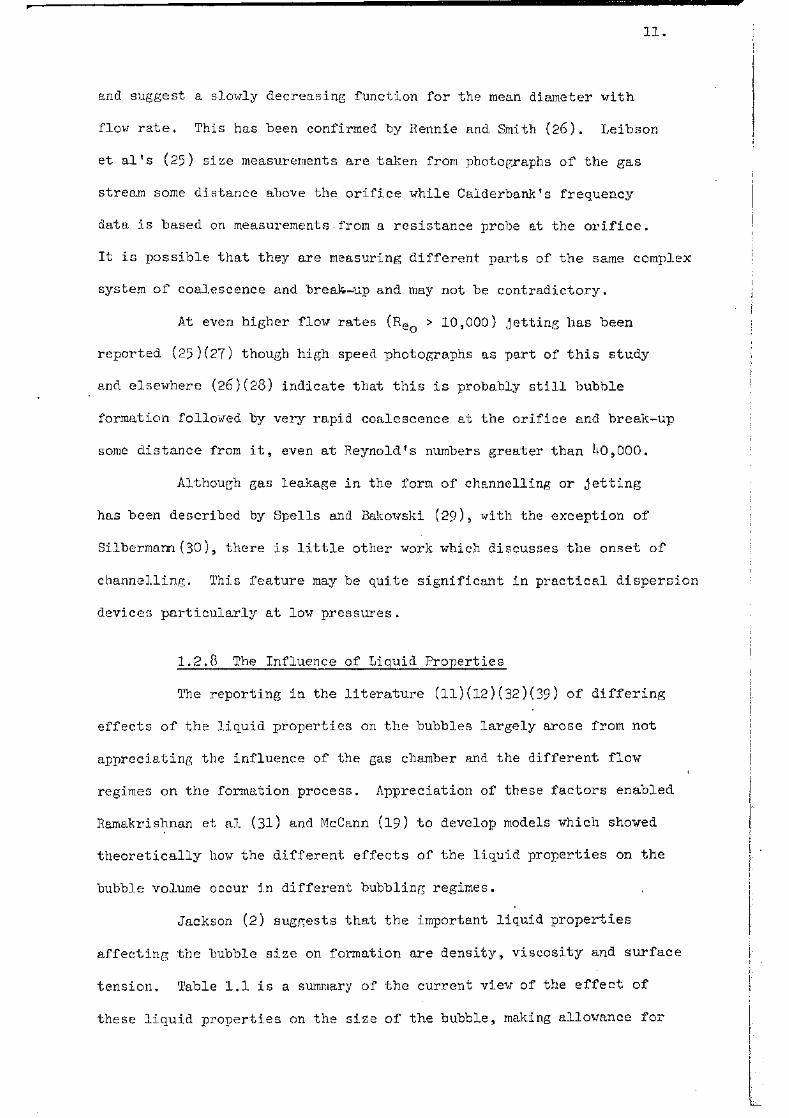
1.2.8 The Influence of Liguid Properties
The reporting in the literature (11)(12)(32)(39) of differing
effects of the liquid properties on the bubbles largely arose f'rom not
appreciating the influence of the gas chamber and the different flow
regimes on the formation process. Appreciation of these factors enabled
Ramakrishnan et al (31) and McCann (19) to develop models which showed
theoretically how the different effects of the liquid properties on the
bubble volume occur in different bubbling regimes.
Jackson (2) suggests that the important liquid properties
affecting the bubble size on formation are density, viscosity and surface
tension. Table 1.1 is a summary of the current view of the effect of
these liquid properties on the size of the bubble, making allowance for

12.·
the flow regime and gas chamber. A positive effect means, other para.-
meters remaining constant, that the bubble volume increases as some
power of the particular parameter, vrhile a negative effect indicates a
negative power of the parameter.
TabJ.e 1.1
-Regime Viscosity Surface Tension Density ~ Static No effect Positive Negative
Region (22) (24) (32') (33) ( 31) ( 33) ( 3h) ( 35) (22)(21~)(32)
----------- ------------·------·------- ---------------------- ---------·-----
Dynrunic
Region
l1 < 200 cp
Small
Positive
(llf) (21) (22) (34)
(32)(36)(37)(38)(39)
l1 > 500·cp
Positive
(11)
Little effect
for constant gas
flow rate
( 31) ( 39)
Positive effect
for constant
pressure(ll)(12)(19)
1.2.9 The Influence of Gas Properties
Negative
( 31) ( 39)
There is little information on the influence of the physical
properties of the gas, since most investigations have dealt with air-
water systems at atmospheric pressure (2). Davidson and Schuler (11)
showed analytically that a 1% decrease in bubble volume should result
from the increased density from air to C0 2 by allowing for the effect
of this density change on gas momentum and the orifice discharge coeffi-
cient. Experimental values by the same workers showed a slightly greater
effect of 1.8% for gas flow rates in the dynamic region.

13.
However Benzing and Myers (24) observed no difference in volume
between air and H2 bubbles at constant flo-vr rate vrhile ignoring data for
C02 bubbles. It is doubtful that the means they used to measure the volumes
would have been accurate enough to observe an effect of the magnitude
estimated by Davidson and Schu1er. A dependence on gas density should
be found since the density effects the chamber capaci tancc -vrhlch a.ffect.fj
the flow into the bubble.
Ifo gas property other tho.n density has been shown to be of
importance, although IG.ing (!tO) suggested that !:Jome discontinuities in
his data may be explained by friction at the neck of the formi.ng bubble,
a phenomena which would be expected to depend on the gas v:i.Dcosity.
Despite this it is common practice to correlate volume and frequency
against orifice Reynold's number which involves gas viscoaity (8)(~'.5).
1. 2.10 Gas ~1omentum
Most theoretical analyses of bubble formation have neglected
the momentum of the gas issuing from the orifice, demonstrati.ng that
it is insignificant for low flow rates at atmospheric pressure. CollinE3
(28) increased the momentum of the gas by increasing the gas velocity.
He concludes that for high flow rates (up to 43 litre /s per orifice)
the motion of the bubble may still be calculated by assuming that it is
governed by inertial, buoyancy and momentum forces. A similar conclUf>ion
was reached by vlrai th ( l+l).
Alternatively the momentum of the gas may be altered by incr<::ns:i.ng
the gas density. Kling noted (40) that the effect of gas moment tun is
quite noticeable for different gases even at very small flo¥r :t'ates. For
a gas flo1-r rate of l.l~ em 3 Is helium :formed perfect spheres during formation,
whereas the ten times more dense argon exhibited a distinct bulging. Only
at a flo'\lr rate of 12 cm 3 /s did the helium bubble distort.

' ' .·--v-/-/\
ONE CONTINUOUS STAGE
SEQUENCE PROPOSED BY DAVIDSON AND SCHULER ( 11)
+ EXPANSION STAGE DETACHHENT STAGE ·I SEQUENCE PROPOSED BY KUMAR AND CO-WORKERS ( 31)
BUBBLE FORMATION SEQUENCE
FIGURE 1.4

14.
1. 3 'I11eore:!J_£:~ t~odels
Although experimental studies of bubbles have been made for
quite some time it is only recently that ·\·rorthwhile theoretical models
have been produced for other than the static region. At present, this
development is limited to models for single bubble growth in the dynamic
region.
The general approach is to formulate an e~uation of motion
involving the forces on the gro~oling bubble and to solve this simultan
eously with an ener~J equation, usually a modified orifice equation.
Davidson and Schuler (11)(12) assumed that gas is supplied
to the bubble from a point source within the liquid as if the orifice
plate were not present. The formation process occurs in one continuous
stage as illustrated on Figure 1.1~ The upward motion of the bubble is
determined by a balance between buoyancy and the drag caused by the
viscosity and inertia. An orifice equation, modified to include the hydro
static and surface tension pressures, is suggested for calculating the
gas flovr rate into the bubble. The change of radius and distance of the
bubble above the orifice with time results from a simultaneous increme11tal
solution of these two equations. The approach is discussed further in
Chapter 8.
An alternative approach has been developed by Halters and Davidson
( 36) ( l~2) who applied potential flovr analysis to the initial motion of two
and three dimensional bubbles. Similarly L'Ecuyer and Murthy (5) determined
the flow'field around a translating and expanding bubble, including the
effect of the inertia of the liquid immediately surrounding the bubble.
Jameson and Kupferberg (20)(43)(41:) and :McCann a.nd Prince (19)
( 45) developed the potential floi·T approach further by making allowance
for variable gas chamber pressure. They applied. their model to a wide
range of orifice diameters and gas chamber volumes with the models giving

t.J
15.
satisfactory prediction of"' terminal volume. To obtain a tractable
solution using this approach a. very idealised picture of the liquid
surrounding the forming bubble must be assumed. Even so the solution
of the resultant equations is tedious.
At the same time as the potential flow approach was being devel-
oped, Kumar and co-vrorkers (15) (17) (31 )* modified the force balance approach
of Davidson and Schuler (12). Instead of the one formation stage they
divide the formation process into two parts based on experimental observ-
ations of Siemes ( 1~8). The first stage is an expansion stage during
which the bubble base remains attached to the orifice while expanding.
The end of the expansion stage is said to be reached when the upward
forces equal the down1-rard forces. After this point the bubble lifts off
the orifice. During the second stage there is a net up1-rard force on the
bubble which rises from the orifice but still expands, being fed by a neck
of gas attached to the orifice.
The two stages of formation are illustrated on Figure 1.4.
The difference between this approach and that of Davidson and Schuler (12)
is apparent. The solution of the equations for each stage of the model
of Kumar and co-·workers (15) (31) is by a trial and error procedure for
the volume at the end of each stage. The solution is less complex than
the incremental approach of the other models. Further discussion of this
model will be made in Chapters 3 and 7.
1.4 Conclusions
A review of the literature indicated that a great number of
reported studies on gas bubble formation in liqui-d systems have tvro common
features; the extensive use of the air-water system and the almost exclusive
use of system pressures near atmospheric. For these conditions and low
* Throughout this -vrork the model developed hy Kumar, R., Ramakrishnan, S .. , Satyanarayan, A. and Kuloor, N .R.) as joint authors in a series of papers ( 15) ( 17) ( 31) ( l-16) ( ~·7) will be ~rouped as "Kumar and co-vrorkers ( ) ", with the specific reference in parenthesis, and the model referred to as "Kumar's model".

flo1-r rates there seems to be some measure of agreement ,provided the
interaction between the forming bubble and the gas supply system is
properly characterised.
16.
There appears to be little systematic study of the turbulent
region of' bubbling - the region of most industrial interest. Nor is
there any attempt to relate the instantaneous volume predicted by the
model to the experimental volumes or surface area.
The influence of gas properties, particularly the gas density,
on the formation process has not been fully investigated for bubbling
systems other than those at atmospheric pressure.
1.5 Scope of the Proposed Study
'I1he conclusions from the review of' the literature pointed to
several areas where useful research could be carried out. As it was
only possible in this work to investigate in depth one of these aspects,
it was decided to study the effect of gas properties on the btilibling
behaviour through increased system pressure.
In many practical dispersion devices one or both phases ha.ve
properties markedly different from those of the air-water system. A
frequent situation arises where the operatine pressure is substantially
different from atmospheric pressure. In this situation, industrially
important gas mass flow rates, although in the turbulent region, should
be obtained at relatively low gas velocities owing to the increased gas
density. A study of the effect of system.pressure on the behaviour of
gas bubble formation would be a useful addition to the experimental
knovrledge in the field.
In order to predict the growth theoretically,previous workers
have justifiably neglected the gas momentum and the effect of gas properties.
At higher system pressures the validity of these assumptions should be
tested andr; if necessary, modifications to existing models or a new model

THEORETICAL RESULTS AND DISCUSS ION
1, SURVEY Of FIELD
/ 3. ADAPTING A MODEL
EXPERIHENTAL
2. EXPERIMENTAL
APPAPATUS
4. INITIAL STUDY
5 I INTE EPRETATION
OF DATA ~ ~--------------~--------------~
7. APPROACH TO MODELLING AND CRITIQUE OF ADAPTED MODEL
6. RESULTS OF
INITIAL STUDY
B. A MODEL FOR GAS BUBBLE FORHATION AT
ATMOSPHERIC PRESSURE
9. A MODEL FOR GAS BUBBLE FORMATION WITH VARIABLE GAS CHAMBER PRESSURE AND GAS MOMENTUM
10, EXPERIMENTAL AND THEORETICAL RESULTS OF A STUDY OF C02
BUBBLING AT INCREASED SYSTEM PRESSUP.£S
11. DISCUSSION OF
PROPOSED MODEL
12. CONCLllS!t1l{S
LAYOUT OF THIS WORK
nGURE 1.5

17.
could be proposed.
Prediction of the type of bubbling ei the:r· empirically or
theoretically vmulcl be a step towards full classification of bubbling
systems.
Figure 1. 5 is a diagrammatic representa:ti.on of the inter-
relation between the various sections of this -vmrk.

FROH
GAS --~~~-t
, CYLINDERS
2
1. CAPILLARY
15
16
3
2. DIFFERENTIAL PRESSURE GAUGE
3. NEEDLE VALVE
4. DIFFERENTIAL FLOW CONTROLLER
5. LIQUID DRAIN VALVE
q. HATER INLET VALVE
'7. FILTER
B. LIQUID Ot.rrLET VALVE
9. GAS CHAl-ffiER
4
14
II
8 9
5
12
....... --,
10.
11.
12.
13.
14.
15.
16.
17.
I r-
1 " { I 10 \. /
T I I
PRESSURE TRANSDUCER
BUBBLE CHAHBER
MANOMETER
PRESSURE RELIEF VALVE
GAS OUTLET VALVE
WET GAS METER
PPESSURE GAUGE
PRESSURE GAUGE t
DIAGRAMMATIC LAYOUT OF THE EXPERIMENTAL APPARATUS
FIGURE 2.1

' I N . ..:I
N
~ t! ~ 5 H t! p:; r&l
~
18.
CliAP'JlJ!:H 2 ----·----:eXPERI1-1EWI'J\.L A PPARAr.rus
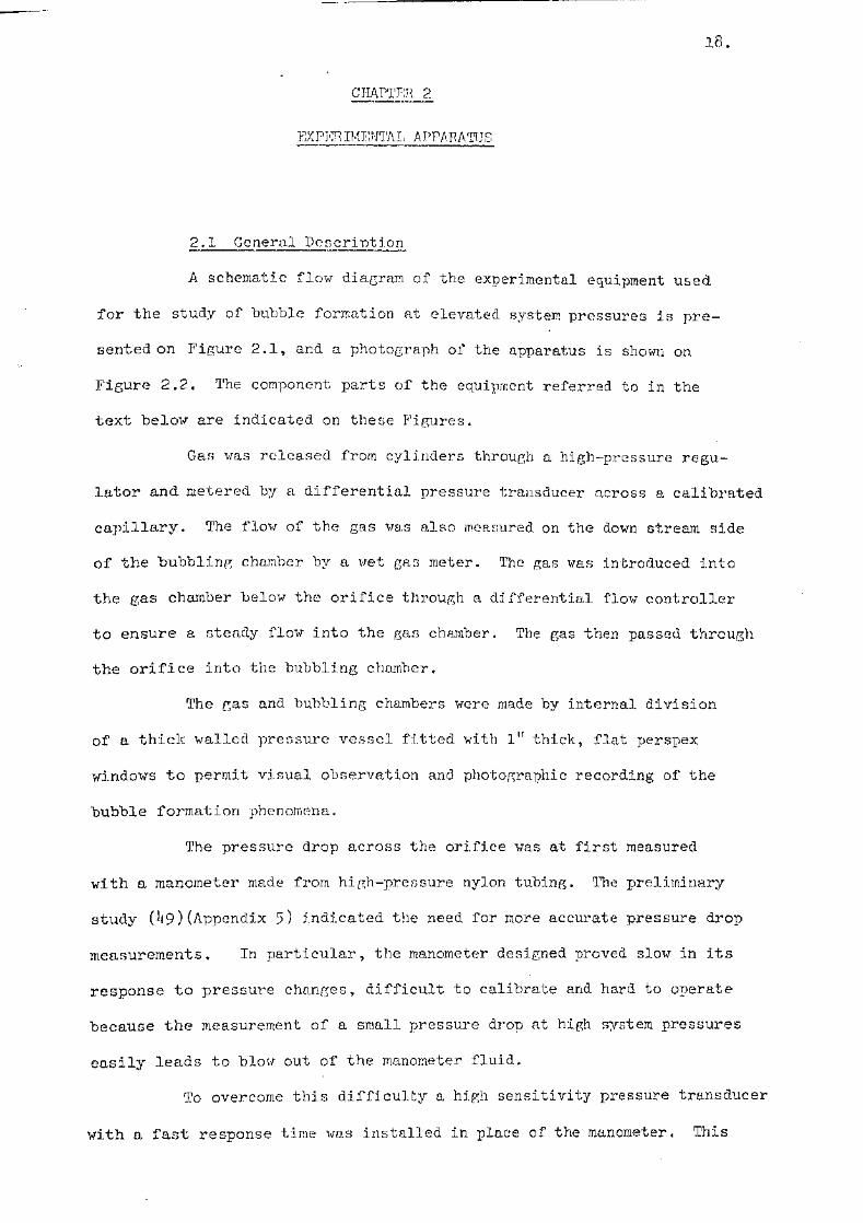
2.1 General Description
A schematic flow diagram of the experimental equipment used
for the study of bubble formation at elevated system pressures is pre-
sented on Figure 2.1, and a photograph of the apparatus is shown on
Figure 2.2. 'I'he component parts of the equipment referred to in the
text below are indicated on these Figures.
Gas '"as released from cylinders through a high-pressure regu-
lator and metered by a differential pressure transducer across a. calibrated
ca])illary. The flow of the gas vras also mea[:ured on the down stream side
of the bubblinp; chamber 1)y a \·ret gas meter. The gas was introduced into
the gas chamber below the orifice through a differential flow controller
to ensure a steady flov into the gas chamber. The gas then passed through
the orifice into the bubbling chamber.
The e;as and bubl)ling chambers 1·rere made by internal division
of a thick walled prensure vessel fitted with 1" thick, flat perspex
windows to permit visual observation and photop;raphic recording of the
bubble formation phenomena.
r:t:he pressure drop across the orifice was at first measured
with a manometer made from high-pressure nylon tubing. 'llfle preliminary
study (49)(Appendix 5) indicated the need for more accurate pressure drop
measurements. In particular, the manometer designed proved slow in its
response to pressure changes, difficult to calibrate and ho.rd to operate
because the measurement of a small pressure drop at high system pressures
easily leads to blow out of the manometer fluid.
r~eo overcome this di:fficulty a high sensi ti vi ty pressure transducer
with a fast response time was installed in place of the manometer. This
GAS OUTLET
BUBBLE. CHAMBER
WATER DISTRIBUTOR r.===::r::l====il L----------,-..-----
~-----1 -- - - -u-------\
PRESSURE TAPPING
(HIGH)
GAS INLET
PRESSURE VESSEL USED FOR EXPERI~~NTAL STUDY (HALF SCALE)
GAS CHAMBER
ORIFICE PLATE (FULL SIZE)
FIGURE 2. 3
WATER INLET

H
~ $1 ~ g 00
g "1\1 H ~ ~ ~ tEJ 1\) ~ . I:"
t::1
0 ::0 H
~ ~ "'d
§ 00

19.
enabled pressure fluctuations during the formation of each bubble to be
followed on an oscilloscope, the results of this particular phase of the
work are reported in Chapter 10. A high capaci t~nce across the input to the
oscilloscope allo\·red the mean prc~ssure readings required in Chapters 4
and 6 to be measm~ed.
The pressure in the bu"bb.ling chaml)er and upstream from the
flow controller were measured 1-d.th calibrated Bourdon tube pressure gauges,
as indicated on Figure 2.1 The system pressure was increased in the
bubbling chamber by throttling back the exit valve which, for safety,
was in parallel with a spring loaded relief valve. The pressure vessel
was surrounded by dou1)le perspex safety screens.
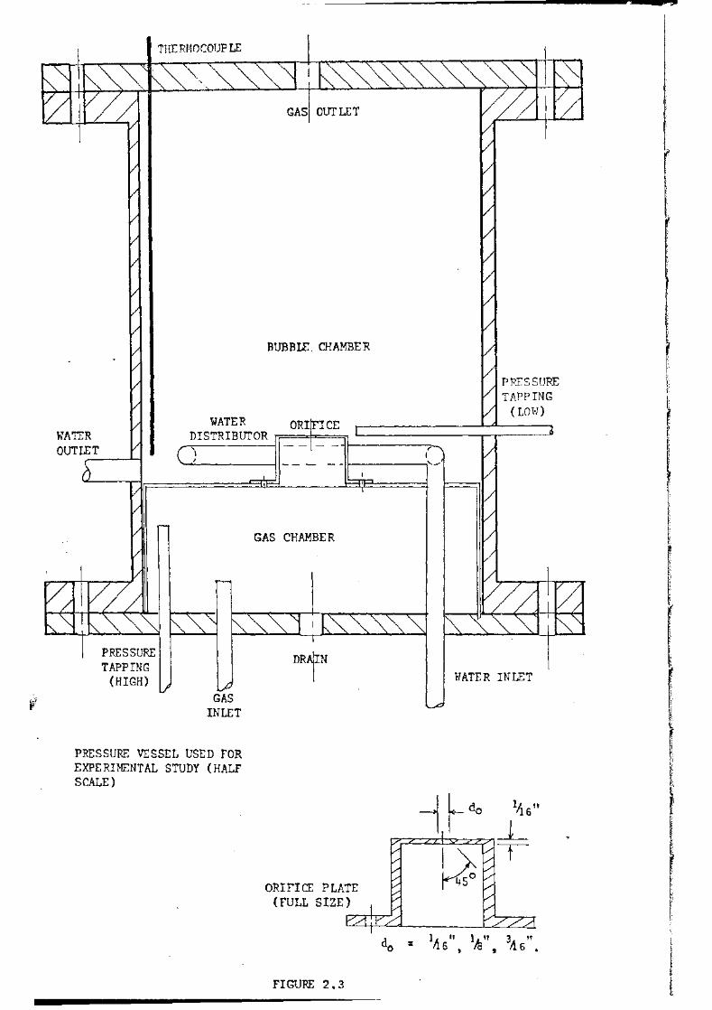
A detailed diagram of the pressure vesse.l used in this ,.m:rl{
is given in Figure 2.3. The vessel consisted of a 4 in. dia. x 12 in.
section of schedule 80 stainless steel pipe, flanged at each end with
~ in. plate. Cover plates were bolted to each end. Extensions were built
into the side o:f the vessel to house the perspex windows, which -v:·E::re made
flat to avoid photograph{c distortion.
The pressure vessel was divided into bubbling and. gas chrunbers
by an internally constructed gas chamber made out of stainless steel
plate which had an interchangeable orifice plate. The internal gas
chcunber and orifice plate are sho-vm on Figure 2. 4
g.2 Orifice Sizes
The orifices used in this work were 11.6", 1/a" and 316" diameter.
The dimensions of the orifice plate are given on Figure 2. 3 The orifice
plate was raised above the base of the bubbling chamber with the object
of minimising the effc~ct of the circulating liquid. svreepi11g across the
orifice.
The calibration of' the orifices to determine the orifice co
efficient is detailed in Appendix 2.

20.
2. 3 Ancill;:;~:!~f Eguinment
A Hedlake Laboratories I!Hycam" high-speed mot:!.on pj.cture camera
vras used to film the formation processes using Kodak Tri-X reversal
black and white 16rnm. film at speeds between l~OO and 2, 000 frames per second.
r:rhe crunera had a neon timing light, capable of cycling at rates of 10,
100 or 1, 000 :per second \vhich focused on the side of the ftlm for a time
base. The camera was also provided \vith an adapter to accept simultaneous
framing and streak recording from an oscilloscope.
A Xenon flash with an output of 7~ };:watts was used as focussed
front lighting into the bubbling chamber while four Philips Photo-Floods
were used as a diffuse backlighting.
A Vanguard Motion Analyser was available for examining the
processed films. This bad the facility for data logging the X and Y
dimension co-ordinates frame by frame from the film. This vras used in
conjunction with the methods for calculating volume and surface area
d.iscussed in Appendix 2 .
2.4 Experimentai Technia~
Small traces of surface active agents~ such as greases, can
cause changes in bubble size (50) (51) (52). To eliminate this as much
as possible the vessel was cleaned carefully with methanol before a
series of runs then rinsed thoroughly -vri th the test water, The water
used was filtered tap w·ater.
Anderson and Quinn (53) have pointed out that even tap water
may cause slightly differing results from day to day. Consistency of the
experimental results and the natural purity of the water indicate that
this effect was not marked in the work reported here.
To carry out a run, C02 was passed through the orifice at
atmospheric pressure, then the bubble chamber filled with water to the
required depth. The pressure was then gradually increased in the pressure

21.
vessel by throttling back the exit valve. Arpressure drop of about
50 psi ~oras maintained across the flovl contl''oller so that the volume of
the gas chamber below the orifice vrould be the same in all cases ..
After sufficient time had elapsed for the water to become
saturated 1-ri th gas, the bubble stream -vras photographed as the flow rate,
pressure and temperature -vrere moni tered. The films vere then analysed
by the methods discussed in section 5.3 and in Appendix 2.

22.
AN ADAPTION OF 1\IJ EXIS1fiiJG rrHEORErriCAL HODEL FOR
VARIATION 0}"' SYS~r.E:T-1 PRESSURE
3.1 Introduction
A broad survey of the literature in Chapter 1 established
a need to examine the behaviour of gas bubbling systems at high pressures.
Available models and correlations should be tested for response to
variation of the system pressure.
The first objective of this ivork was to undertake an exploratory
study of high-pressure bubbling to elucidate the areas where problems
might arise and to indicate the direction tha.t the main study should
follo-vr. This initial work, both theoret:.ca.l and experimental, is cov
ered in Chapters 3 to 6.
In this cha"Pter an existing analytical model for predicting
the voltnne of gas bubbles formed at a submerged orifice is adapted to
account for the variation of gas properties with increased system pressure.
3.2 Literature Related to Estimatinf£ the Effect of Variable
System Pressure
3. 2.1 Ass1.:unpttons at Atmospheric Pressure
In analysis of data obtained at atmospheric pressure two
sim:plifing assumptions are normally made:-
(a) Gas properties have a negligible influence on the
bubble growth.
(b) Gas momentum is negligible.
Both these assumptions are justified at atmospheric pressure but are
of decreasing validity as the system pressure is increased.

23.
J.2.2 Gas Properties at Atmosnhe:ric Pressure
Although gas properties are considered in some studies at
atmospheric pressure (8)(24)(25) there is no evidence to suggest that
they significantly affect the bubble formation process. There is little
justification for the inclusion of gas properties in correlations (2).
3.2.3 Gas Momentum at Atmospheric Pressure
Davidson and. Schuler (11) suggestecl that the expression,
p 'Q2 , may be used for the rate of change of gas momentum issuing through
Ao
the orifice. For a gas flow rate of 1 cm3/s at atmospheric pressure,
Davidson and Schuler (11) found that this expression for the momentum
of the gas accounted for only 0.5% of the upward force on the bubble ..
In the work reported here, where high pressure bubbling of C02 is studied,
the rate of change of gas momentum can make a significant contribution
to the upward force on the forming bubble. Calculations presented in
Appendix 3 show that for 1 cm3/s, the gas momenttun accounts for 10%
of the upward force on C02 bubbles at 150 psig. and 21% at 350 psig.
Thus an analytical model for increased system pressures must
account for the contribution of the gas momentum to the development of
the bubble.
In a study of bubble formation at atmospheric pressure and p 1Q2
high gas flow rates, Collins (28) concludes that the term, -- , Ao
adequately accountE: for the gas momentum and may be incorporated in
Davidson and Schuler's constant flow model (11) with reasonable success.
This expression for gas momentum has also been employed at
atmospheric pressure by Wraith ( 1.~1) in another study of high gas vel-
oci ty bubbling and by Kumar ( 51.t) in an attempt to relate gas-liquid
to liquid-·liq.uid studies. It will be used in this chapter to account
for the increased gas momentum caused by increased gas density.

INITIAL
CONDITIONS EXPANSION STAGE DETACHMENT STAGE
FORMATION SEQUENCE FOR MODEL DEVELOPED IN CHAPTER 3
FIGURE 3.1
£;
FINAL CONDITIONS

3. 3 rrhe Existin.r.:; Hodel
The model in the subsequent sections -vras developed in order
to obtain a theoretical basis for the analysis of bubbling behaviour
at system pressures greater than atmospheric. It extends the concepts
of Kumar and co-\·Torkers* (15)(31), described in Chapter 1, to include
the variation of gas properties with increased system pressure and the
force due to the rate of change of gas momentum through the orifice.
This model was adapted in preference to the other models
discussed in Chapter 1 for the following reasons:-
(1) Kumar's model* could be readily adapted :for high pressure
situations. Its solution was relatively simple and it
had been successfully applied ( 15) ( 31) over a wide range
of conditions.
(2) Kumar and co-workers (15)(31) had demonstrated that their
model was an improvement over that suggested by Davidson
and Schuler (11) ( 12).
(3) The complexity of the potential flow approach, for instance
that of Kupferberg and Jameson (20), did not appear to
be warranted in the preliminary investigation, especially
if high pressures resulted in greatly increased turbtuence.
It would be difficult to include the gas momentum in this
type of approach.
3. 4 The Assump_ti9ns of the Adapted Nodel
The formation seq_uence analysed is given in Figure 3 .1. It
is assumed that bubble formation taJces place in two stages following
the suggestion of Siernes and Kaufmann (48). During the first or expansion
stage the bubble grows -vrhile its base remains attached to the orifice.
In the second, or detachment stage, the base of the bubble moves away
from the orifice while it is still growing, but remains connected to
* See foot-note, page 15.

25.
the orifice through a neck of gas.
The model assumes that:-
(1) The bubble is spherical throughout formation.
(2) Circulation of the liquid is negligible, so that the
liquid s1.rrrounding the orifice is at rest -vrhen the bubble
starts to form.
( 3) The motion of the bubble is not affected by the presence
o:f another bubble irrm1ecliately above it.
( 4) The inertia of the liquid surrounding the bubble may be
accounted for in the virtual mass of' a sphere moving
perpendicular to a wall (11)(55).
( 5) Interaction between the bubble and the gas chamber pressures
is negligible. That is, bubbling is assumed to occur
under constant pressure conditions (11). A check on
this simplification for the experimental system has been
made by calculating the capacitance number, Nc, given by
Hughes et al ( 1~) which characterises this interaction.
For a 1/1 6" orifice a.nd a gas chamber volume of 375 em,
Nc decreases from a value of about 50 at atmospheric
pressure to 1 near 350 psig. Constant pressure behaviour
may be assumed when Nc>>l ( h ) . McCann (19) has shOim
that this may not be a sufficient criterioq, but for the
preliminary investigation reported in Chapters 3 to 6,
constant pressure will be assumed despite Nc+ 1 at higher
system pressures. Subseq_uent chapters will cleal with
the problem of variable gas chamber pressure.
(G) The only gas property that needs to be considered in
mbdelling for increased system pressure is the gas density.
It has been shown that the gas density at increased system
pressure contributes to the upward forces on the bubble

26.
through the gas momentum. It also has an appreciable
affect on the buoyancy and virtual mass of the bubble.
The gas viscosity for the pressures studied (see Appendix
I) shows negligible variation from the value at atmcs-
pheric pressure) where the literature (2) shows it can
be neglected.
3. 5__!J)e Eauation for Flo-vr int<? the Forming Bubble
Variation of volumetric flow rate through an orifice can be
expressed by an orifice equation (56). For any particular orifice,
assuming that the effective area of discharge of gas into the liquid
is the Sffine for all gas densities and equal to the orifice area, the
orifice equation may be expressed as:-
Q ::: K 3.1
(p t )~
K is the orifice coefficient determined experimentally for the flow
of gas through the dry orifice. K is assumed to be unchanc;ed 1-rhen the
gas bubbles into the liquid.
Davidson and Schuler (11) have suggested that the pressure
drop across the orifice, t.P, as the bubble is forming may be expressed
as:-
V• K (P h 2cr)~ Q. ::: = - 1 - p g + p ga, - - 2
(p'r~ . a 3.2
This expression makes allo-vrance for the height of the centre
of the bubble above the orifice and for the pressure :required to maintain
the interface.
3. 6 'l11e Exnansi on Stage of Formation ( 15)
3. 6.1 The Existing Eouation for._ the First StaP;:e.
During the first stage of the formation process the bubble

27.
gro;;.,rs with its base attached to the orifice. The upward force caused
by the buoyancy has to overcome three resistances; viscous drag~ liquid
inertia and surface tension. The bubble base remains attached to the
orifice until the buoyancy force exceeds the do~m-vrard force.. The force
balance to mar}~ the end of the first stage J?ro:posed by Kumar and co-
workers (15) is:-
Bouyancy
dt
Inertia Surface Viscous Tension Drag
3.3
The viscous drag (Stoke's law) is valid only for a sphere
moving at a constant velocity with lovr Reynold's number. A more general
approach is given by Bird et al (57)) but substitution for the viscous
drag in this form would cause a considerable increase in computational
complexity which -vras not considered justifiable, particularly vrhere
provision for a gas momentum term must also be made.
3. 6. 2 Allo;;.ring for Variable Gas Properties and Ga.s Momentllll}
The force balance used to describe the end of the first stage,
equation 3.3, assumes that the gas is supplied continuously at a point
source which is always located at the centre of the expanding bubble.
The term for the inertial forces due to expansion does not
include the effect of the added gas per unit time. This may be derived
by considering the motion of the bubble as a variable mass probJ.em.
This analysis is presented in Appendix 3. It is shown that the effect
of the added gas may be expressed as the rate of change of gas momentum
p 'Q2 as it is blown through the orifice, ~' as suggested by Davidson and
Schuler (ll). A0 is the effective discharge a:rea of the orifice ~orhich,
as for the orifice equation, is assumed equal to the actual orifice
area.

28.
In the experiments reported here the gas momentum acts in 'the
same direction as the buoyancy. It thus has the effect, as its valu.e
increases, of taking the bubble from the orifice at. an earlier stage
of formation.
The gas density must be included in the buoyancy term and in
the expression for the virtual mass of the bubble~
M = VE (p' + ~) 3.4
This value of virtual mass applies strictly to a completely inviscid
liquic;l and should be regarded here as only giving an order of magnitude
of the inertial effect (11)(55).
3. 6. 3 The Adanted. Eg1Jation for the First Stag~
With the inclusion of the gas density and momentum, eq_uation
3.3 becomes:-
+ 3.5
Following the development ot: Kumar and co--vrorkers ( 15) by substituting
for QE by using equation 3.2 into equation 3.5 and usinB,
1 3.6
which relates the bubble radius to bubble volume,
and, dvE ::: M-- + VEdM
dt dt
the final force balance for the end of the expansion st~:Lge is:-
4 2 ' K 2 ( p ' + 1-k ) 2o ) V E ( p - p ' ) g + = JlL ( p + p gaE - -
Tido 2 aE p 1 411' aE ·
3.8

29.
where P = P1- pgh.
3v liJ Expressing aE as (
4!) equation 3.8 is solved by trial
and error for VE, the volume of the bubble at the end of the first
stage.
3. 7 The Detachment Stac;e of Format ion ( 15)
3. 7 .l rrhe Existing Hodel for the S~cond Stage
In the second stage of gro\·rth Kumar's model supposes a net
upward force vrhich accelerates the expanding bubble from rest. In
order to evaluate the final bubble volume, VF, Kumar and eo-workers
(15) assumed that the flo-vr rate during this stage was constant and
equal to QE, the flo~or rate at the end of the first stage. This simpli-
fication was justified from consideration of the flow equation,
Q = K (Pl - pgh + pga - 2cr)~ ~2 Ct
3.2
Computations based on the adapted model used for the present work
justify this conclusion.
As a consequence of this assumption, during the detachment
stage the volume is thus given by V = VE + %t, and the equation of
motion of the bubble by:-
d(Mv') 2
(v + ~t) ( P I )g + l~QEp' 6 t d = E p - - na~v - n 0 cr nd 2
0 dt
where v' is the velocity of the centre of the bubble and is made up
of the velocity of the centre due to expansion and the velocity with
which the bubble base is moving, that is,
v' = v + dct dt 3.10
Detachment is assumed to take place when the bubble base
has moved a distance equal to aE, the radius of the bubble at the end
of the first stage. Kumar and co-workers (31) suggest that this corre-

30.
ponds to the condition where t.he rising bubble is not caught up by
the next expanding bubble.
The solution of equation 3. 9 :t'ollo'ivs that given by Kumar and
co--worker:s (15). 'rhe final equation for detachment, including gas
properties, is:-
where,
and
3G (V ~ V 2.3) 3E (V 113 V V3) ( r:::) 't1, - E - ( 2A) F - E 2QE A-.Yj .{' Q A·- .J
1 (V -A+l -A+l) I( B )• A+l (C)V A Q(-A+l) F - VE A+1 lf:rr; . - A E
3.11
3 113 ¥3 A = l + 61r ( 1'4n) VJi~ 1. 25l1
B =
c =
E =
G =
QE(P' + w) (p- p')g_
(p '+JJ.o )Q lt)' E
2 ( 3 ) 113 ( '+ ~ ) Ij."'; p .L () '
Kumar and co-workers (31) made further simplifications of
eq_uation 3.11 by eliminating the last two terms which vrere claimed

31.
n.t
of the ClJTrcnt ::;t;ud.v ru11l it "~:ms a rr~lat:ivc1;r eo.s:r matter to inco.r· Q
the termD :in a :r_:rrog:r·run for a c.l1g:ttal corz1puto.r.
Equation 3.11 :t s solved lJy trinJ. a.ncl error :f.'ur V:F'.. rn1e
computor programme p:cc::·.ented in Append:b\ l1 to solve tht:.~~~e equat:i. ouG
presented by Kumar nnd co-workerf1 ( 15) an<1 va::: fouilcl to be in ar;r<?I.::Hwnt ..
3 . 8 Sumrn t.1l''V .:------·-n-.J.,.., ...
has been ·proposed 'b;r t:=tld.ng an n.vaile .. ble model for atrnoD f.lh(;rie :prcn:>GU:t'e
and adapting it for va:r:·iation in gas denG:i.t.:v and makinr~ f.1,llo"';.;ance for
the effect of gas momentum.
As the c;ac; rnornentum te:r.·m contributeD to the upHard i'orcr: on
the bubble i.t is expected tl10.t increased gan density """'ill cau~1o ::m~alJ.er '
bubbles to be formed r..tt the or:i. fi er.:.', :i. f tr1e voJ.umetri c fJ.o·vr rate i G he1cl
constant.

32.
CHAPTER 4 -------INI':.eiAL S~TIJDY ON 'I'HE 1-:FFEC'T OF SYST.FA-1 PRESSURE
4.1 Summary ------·-1-This chapter reports an explorato:t"'y experimental study of
formation of carbon-dioxide bubbles at a single submerged orifice in
water at system pressures from 0 to 300 psig.
It demonstrates that the bubble size, frequency and shape at
elevated pressure differ from that encountered at atmospheric pressure.
'l1he results of this study are compared with the adapted model
developed in Chapter 3. From this comparison several anomalies between
theory and experiment are apparent. It is concluded that, both a re-
examination of the data, and an a.::::1sessment of the criteria for bub1;le
termination are necessary.
l1. 2 Literature Related to the F.xnerimentn.l Investigation
A study of absorption of C02 in water under pressures up to ~
450 psig has been made by Houghton, McLean and Ritchie (58) using a gas
bubble column of small diruneter with a multi-hole gas distributor. It
was found that the efficiency of absorption decreaseo: with increasing
pressure but they were unable to satisfactorily explain their results.
Changes in bubbling behaviour with increased pressure were not con--
sidered as a possible explanation.
Kling ( 4o) in a paper on the dynamics of bubble formation
under pressure points out that gas contacting devices, such as sieve
trays, tested at normal pressure possessed quite different operating
characteristics at high pressures. The results were compared at constant
volumetric flow rate.
The study made by Kling (40) covers the behaviour of a variety

33.
of gases at low flow rates (1 to 12 cm3/s) at pressures from 0 to 1200
psig bubbling through orifices of 1.05 and 1.6)-+ mm. diameter. The
paper suggests that the increased gas momentun1 decreases the size
and distorts the shape of the formed bubble. However it of'fers·no
analytical evaluation of this effect.
It. vrould appear that no literature references are available
for bubble formation from an orifice at higher pressures~ although
Grigull and Abadzic (59) ( 60) have presented interesting photographs
of boiling C02 on a thin heated wire at pressures near the critical
point;
1"'he preliminary studies on -vrhj ch this section is based have
been reported by La Nauze and Harris ( ~·9) (see Appendix 5) in a paper
on the effect of system pressure on the behaviour of gas bubbJ_es formed
at a single submerged orifice. The :paper shm·red the importance and
the effect of the increased gas density on the formation process.
Further investigat:i.on has lead to some modification o:f the results
presented in that paper.
4.3 Range of Conditions Studied
The followine; experimental conditions w·ere used in the study
reported in this chapter:-
Gas Carbon-dioxide
Liguid Water
S;;[stem pressure 0.- 300 psig.
VoJ.umetric flo\·r rate 5,10,15 cm3/s at system pressure
2" above orifice
Orifice diameter 1;16 11, sharp edged orifice
Carbon-dioxide was chosen as the gas because of its high
den'sity and compressibility. It vou.ld also provide data on a system
other than air-water.

,,
A. ATMOSPHERIC PRESSURE B. 150 psig
Conditions: C~/Saturated Water
Orifice Diameter 1/16"
Liquid Seal 2"
c. 300 psig
GAS BUBBLE BEHAVIOUR FOR CONSTANT VOLUMETRIC FLOW-RATE OF 5CM 3/S At SYSTEM CONDITIONS
FIGURE 'J.l

A. A'll-fOSPHERIC PRESSURE B. 150 peig
Condi tiona : C~/Saturated Water
Orifice Diameter 1/16"
Liquid Seal 2"
c. 300 peig
GAS BUBBLE BEHAVIOUR FOR CONSTANT VOLUMETRIC FLOW-RATE OF 10CM3/S AT SYSTEM . ·cONDITIONS
FIGURE 4.2

A. A'IMOSPHERIC PRESSURE B. 150 peig
Conditions: C~/Saturated Water
Orifice Diameter 1/16"
Liquid Seal 2"
c. 300 psig
GAS BUBBLE BEHAVIOUR FOR CONSTANT VOWMETRIC FLOW-RATE OF 15CM3/S AT SYSTEM CONDITIONS
FIGURE_, 4 • 3

3h.
The range of pressure used covers a change in the ratio of
liquid to gas density from 500:1 at atmospheric pressure to 20:1 at
350 psig. This corresponds to a mass flow rate range of 6.5 x 10⁻⁶Kg/s
to 6. 75 x 10-4Kg/s, at the volume flo-vr rates quoted. At high system
pressures industrially important mass flow rates are achieved at corn-
paratively low gas velocities. Calderbank (8) has suggested that the
flow rates of industrial importance lie between 40 and 270 cm3 /s. at
atmospheric pressure for a single orifice. The volumetric flow rates
chosen for this study lie within this range after correction for increased.
pressure.
The orifice diameter of 116" (1. 59 mm.) was chosen so that a
comparison with the results of YJ.ing (40) might be made. It was also
a multiple of orifice sizes used in many other works (19) (1+3).
Variation of system properties with pressure are given in
Appendix 1. The sys tern was studied at room tem:r>erature vrhich varied
0 from 18 to 22 C .
4.4 Experimental Procedure
The experimental procedure has been outlined in Chapter 2.
The high speed photographs in this section were taken at l+OO f'rarnes/ s.
This is the same rate as chosen by Collins (28) for high gas velocity
bubbling and is similar to filmine; rates chosen by other -w·orkers (11)
( 19) (20). The photographs were analysed on a motion picture analyser
as described in Appendix 2.
4.5 Illustration of Tvnical ResQlts
The photographs presented in Figures 4.1 to 4.3 show the
variation of gas bubble behaviour with increasing pressure for constant
volumetric flow rate at system pressure.
For 5 cm 3/s it is clear that as the pressure is increased

35.
the bubbles become smaller but more frequent, maintaining their separate
identity throughout the range of pressures used. At the hi.gher flow
rates of 10 and 15 cm 3 /s this ini tio.l decrease in volume is also observed.
For these flow- rates, ho~..rever, the rapidly forming bubbles begin to
touch each other in the :pressure range 100 to 150 psig. The bubbles
then form a chain.
As the pressure is further increased distinguishing between
bubbles formine these loose chain structure becomes increasingly more
difficult. To the unaided eye the gas appears to be jetting through
the orifice in a continuous stream.
It :i.s clearly evident that the bubbling process becomes more
complicated as the pressure is increased.
4.6 Interpretation of the Photograuhs
The total formation time of a bubble ha.s been defined by L'Ecuyer
and Murthy ( 5) as the interval of time bet\veen the first appearance of
a gas meniscus at the orifice and the visible detachment of the formed
bubble. 1bis definition was used as a basis for calculating the average
bubble volumes presented in section )~. 7 from the experimental films.
1~ • 7 He s ul t s
The follo-vring graphs are presented, based on the interpretation
of films of the bubbling process:-
Figure l~ • 4 Bubble volume vs. System pressure for 5 cm3/s
Figure 4.5 Bubble volume vs. System pressure for 10 cm3/s
Figure 4.6 Bubble volume vs. System pressure for 15 cm3/s
The curve on these Figures represents the predictions of the adapted
model developed in Chapter 3. A comparison of the experimental results
with those of Kling (l~O) is given on Figure lL 7.

,__ __ o. 8
H---0.7
50 100
co2;saturated Water
Gas Flow Rate 5cm3/s
do = 1/16"
150 200
GAUGE PP~SSURE PSIG
250
EXPERIMENTAL AND THEORETICAL AVERAGE BUBBEL VOLUl1E VERSUS GAUGE PRESSURE
FIGURE 4.4

0.8
0.7
---- 0.3
0.2 (J
0.1
50 100
C02/Saturated Water
Gas Flow Rate 10cm 3/s
do = lf1s"
150 200
GAUGE PRESSURE PSIG
250
EXPERIMENTAL AND THEORETICAL AVERAGE BUBBLE VOLUME VERSUS GAUGE PP£SSUHE
FIGURE 4.5
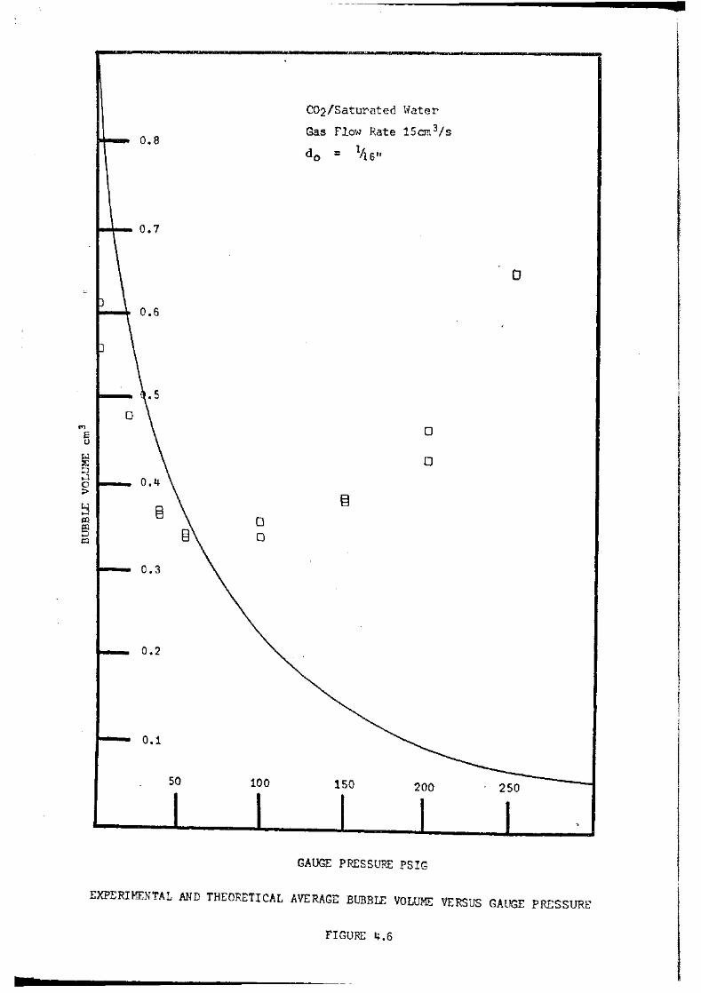
"' E 0
~ B 0 :>
~ ~
f§ t:t.:l
o.a
0.6
0
8 0 0
0.3
0.2
0.1
so 100
C02/Saturated Water
Gas Flow Rate 1Scm 3/s
do = 1/16"
0
0
150 200
GAUGE PRESSURE PSIG
0
EXPERIMENTAL AND THEORETICAL AVERAGE BUBBLE VOLUME VERSUS GAUGE PRESSURE'
FIGURE 4.6

M
E 0
50
This Work
Kling ( 40)
Kling (40)
100
Carbon-Dioxide do = 1/16"
Nitrogen
Argon
..
150 200
d0 = 1.05mm.
d0 = 1.05mm.
250
GAUGE PRESSURE PSIG
COMPARISON OF RESULTS BETWEEN THIS WORK AND KLIN(j ( tt.O)
FOR EXPERIMENTAL AVERAGE BUBBLE VOLUME VERSUS GAUGE
PRESSURE
FIGURE 4.7

~----~----------------------------------------------~--
36.
4.8 Discussion
The photographs of the bu1Jr)les formed a.t the same flm·r rate
but at different system pressures sho-vr that the increased pressure
causes the bubbles to become smaller and more frequent. Tne growth
of the bubble at higher pressures is terminated earlier. The pre
diction of the model on F:i.gures 4.4 to 4.6 follov this trend.
The experimental values of bubble volume for a flm-r rate of
5 cm3/s, F'igure 4.1~, also exhibit this trend as was expected. Com
parison of these results w·i th those of J:Q.ing ( l~o) for two different
gases, Figure 4.7, gave good agreement.
The experimental results for the two higher flow rates, Figures
4.5 and 4.6, show an unexpected deviation from the model predictions.
After the initial decrease in volume with increasing system pressure,
the measured bubble volume appeared to increase.
For this region the experimental films gave the impression
that chain bubbling gradually lost its distinct structure and became
a series of irregularly sized jets which periodically detached. from the
orifice. The jets disintegrated into smaller bubbles after moving a
short distance.
This behaviour is similar to that described by Leibson et al
(25) and Rennie and Smith ( 26) for high gas vcloci ty bubbling~ except
t.hat large numbers of very much smaller 1Jubbles were also observed in
their studies.
In order to maintain the volumetric flow rate when the bubble
volume is decreasing, the bubbles must not only form in a shorter time
but also \vi th a decreasing lapse time bet1-reen them. Chain bubbling is
said to occur ~>rhen the lapse time becomes zero. After chain bubbling
has been established any further increase in pressure vrill lead to a
complex situation of growth and coalescence near the orifice. The

37.
apparent increase in bubble volume occurred soon after the establishment
of chaining.
It is possible that the increase in size of the bubbles could
be explained by the onset of a ne-vr bubbling regime, complicated by
coalescence at the orifice. Alternatively using visible detachment
as a criterion for interpretation of the data may be insufficient
when analysing rapidly formed, close1y spaced bubbles. The reason
for the apparent increase in volume needed clarification before a
worth-vrhile evaluation of the model was obtained. To do this a re
examination of the data was felt necessary.
h.9 Conclusions
This initial study has shown that bubble growth at high
pressure is different from that at atmospheric pressure. When comparison
is made at constant volumetric flo-vr rate increased pressure leads to
a great increase in the interaction between successive bubbles. The
study has sho-vm that size, shape and frequency of bubbles formed at
high pressures are considerably altered from the same characteristics
measured at normal pressures.
However, the results need to be re-examined to resolve an
apparent contradiction between tl'le predictions of the model and the
experimental findings. In particular the criteria used to determine
bubble termination in analysing the films neecl to be :re-assessed.

38.
CHAPTER 5
CRrrEHIA FOR BUBBLE Tr:;:RI,iiiNATIO!f
5.1 Introduction
The initial study descrrbed in Chapter 4 showed that increased
system pres sure caused greater interaction bet"\~Teen successive bubbles
when comparisons 1-rere made at constant volumetric flow rate.
mental resul.ts for bub-ble volume were obtained 1-rhich differed from the
predictions of the model. It was considered necessary to determine
whether this di. screpancy was caused by a change in the mode of bubble
formation or by the interpretative procedure applied to the analysis
of the photographic records.
The simple definition that a visible break in the gas stream
indicates bubble termination is insufficient in the present case where
the time bet\-reen successive bubbles tends to zero tmless the time
between successive photoe;raphic frames also tends to zero.
This chapter deals w·i th the problems involved in interpretation
of the photographic record and develops a set of guidelines to be used.
5.2 Problems Involved in Interpretation of the Results
I'-1any studies of gas bubble formation have used photographic
methods of recording the phenomena occurrine;. Some of the general :prob
lems related to photographic methods are reported elsewhere (61) (62) (63).
The frame rate of 1~00 frames Is chosen for the initial study
is an adequate speed in situations .. ,.,here a definite lapse time greater
than the exposure time per frame exists between bubbles . Hhere tl!e
lapse time ?etween bubbles is small then it is important to remember
that the film is not a continuous record with time. A film gives
discrete exposures of a short duration (the exposiJ.re time) at a given

39.
slOi-Ter rate (the frame rate). For instance, for the camera used in
this study the exposure time represented a value of one fifth of the
:frame rate. That is, for 400 frame/s the film recorded an exposure
of 0.0005 second every 0.0025 seconds.
For high flov rates or high pressures, where both the lapse
time betvreen bubbles and the formation time are greatly reduced, care
must be taken to ensure that the frame rate is such that a sufficient
number of exposures per bubble are taken. In this case sufficient
implies a number that will ensure that the detachment of each bubble
is clearly recorded. That is, the interval of time between exposures
should be less than the lapse time.
For the flow rates and pressures used in the initial study,
the time betvreen exposures was considerably larger than the lapse time
at the higher pressures owing to the increased gas momentum, It was
possible that there vrere not enough exposures per bubble for an accurate
assessment of the bubble formation process.
A more reliable record was obtained by repeating the exper
imental runs using a framing rate between 1,000 and 2,000 frames/s,
thus providing more exposures during each formation period.
The new films showed that many more bubbles- were being formed
than "i-Tas previously apparent. The greatly increased gas momentum was
causing a bubble to coalesce with the preceding bubble very close to
the orifice. Chain bubbling was still the mode of formation and not
jetting· as previously considered. Despite the increase in filming rate
interpretation of the photographs was still not an easy task.
5.3 Guidelines for Interpretat~on of Experimental Data
The complexity of the behaviour of the gas stream passing
through the orifice at high pressures made j.t necessary to deve.lop
a detailed set of criteria for determining when a bubble terminates

(a) (c) (d)
IDEALISED PICTURES OF BUBBLE FORMATION
FIGURE 5.1

CHAINING
Condi tiona: C~/Saturated Water
Orifice Diameter 1/16"
Liquid Seal 2"
Gas Flow rate 1oCM3/s
System Pressure 150 psig
FIGURE 5.2

4o.
and a ne1·r bubble commences to form. A bubble in the accepted ~•ense
terminates when there is a break in the gas stream. If, hm.;ever, the
ga.s momentwn is large, succeeding bubbles commence to grow -vli thout a
perceptible lapse time occurring. In these cases a more difficult
interpretive situation arises.
As an aid to the interpretation of the data consider au
idealised picture of formation, Figure 5 .l(a), which~ for the sake of
this discussion, is assumed reasonably representative of the bubbling
process. If the conditions are such that the gas momentum is sufficiently
high to initiate the grm-rth of' the succeeding bubble without interruption
then this "chaininr; 11 situation might be represented as given on
Figure 5 .l(b).
Since the initial rate of growth of the bubble is slower than
the velocity at which the base of the preceding bubble rises there will
be shearing at the interface between the t-vro bubbles. Depending on the
prevailing physical situation the interface will either stretch and
rupture or elongate into a thin neck but not rupture. Figure 5.1(c)
is a theoretical representation of this latter situation, while Figure
5.2 compares this with an experimental photograph.
This theoretical representation of tne bubbling process,
although an obvious simplification, can act as a useful guide for the
interpretation of the experimental films. If the demarcation between
bubbles reaches the stage of difficulty where a degree of subjectivity comes
into deciding when a bubble has actually terminated, then bearing in
mind this bubbling pattern vill help eliminate subjectivity as much as
possible.
Consequently, as the films have to be analysed frame by frame,
the followine guidelines were used for determining bubble termination:-
( 1) A visible break in the gas stream.
sd

1
11
19
26
1. Visible Detachment.
2. For motion of a ~1enis cus •
3.. Provisional Detachment, confirmed.
3* Provisional Detachment, not confirmed.
Conditions: C02/Hater; 300 psiR, 1/16" orifice, 10cm 3 /sec.
DETERHINATION OF BUBBLE TEPJ.UNATION FOR CHAIN BUBBLING

41.
( 2) The format ion of a meni Be us across the gas stream vras
considered to mark the end of a ·bubble, even though
separation did not occur. The inte:r-fa.ces generally forrr.ed
to accommod.ate sharp changes in surface contour at a
narro1-ring of the gas stream. Often the meniscus existed
for only a fraction of a second before being ruptured
by the up1-rard momentum of the gas forming the next bubble.
Alternatively these liq_uid interfaces persisted as the
bubble continued to rise.
(3) At pressures greater than 250 psi g. a situation arose
in some cases vrhere a constriction in the gas stream formed
close to the orifice but, neither a break nor a meniscus
could be detected. For these cases, if bubbling in a
regular chain was occurring and the constriction matched
this pattern, then the constriction was considered to mark
the end of a bubble, subject to the proviso that no break
or meniscus formed within the next few frames. For these
pressures, this criterion was used for determining the
end of a bubble in about one in every fifteen cases.
To illustrate the use of these guidelines an outline tracing
from a projection o:f a film is presented on Figure 5.3 The case drawn
is for a volumetric flow rate of 10 em 3 Is through a 11 6" orifice at
300 psig. filmed at 2,000 frames/s. Figure 5.3 demonstrates an extreme
example of the interaction between successive bubbles. For the most
part the interpretation of the films was less di.fficult.
The guidelines above have been used to indicate the end of
each bubble formation period, a. numbered l:i.ne on Figure 5.3 indicates
this. The number corresponds to the criterion used, as listed above.

CHAIN BUBBLING GAS JETTING
THEORETICAL COMPARISON OF CHAINING WITH JETTING
FIGURE 5.4
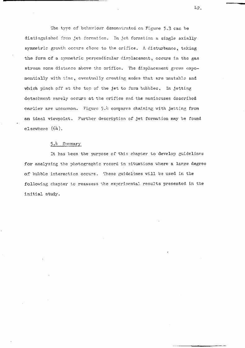
42.
The type of behaviour demonstrated on Figure 5. 3 can be
distinguished from jet f'orm~rt,ion. In ,jet formation a single axially
symmetric gro1.·rth occurs close to the orifice. A clisturbance, taking
the form of a symmetric pen)endicular d.isplacement !'I occurs in the gas
stream some distance above the orifice. 'llfte displacement gro"lfrs expo
nentially with time, eventually creatine; modes that are unstable and
which pinch off a.t the top of the jet to form bubbles. In jetting
detachment rarely occurs at the orifice and the meniscuses described
earlier are uncommon. FiGure 5.4 compares chaining with jetting from
an ideal vie,~oint. Further description of jet formation may be found
elsewhere (64).
5.4 S1J:!]].~Y.
It has been the purpose of this chapter to develop guidelines
for analysing the photographic record in situations v-rhere a large. degree
of' bubble interaction occurs. These guidelines vrill be used in the
following chapter to reassess the experimental results presented in the
initial study.

o.s
0.6
o.s
0.3
.g.2 0
0
MODEL
0 o.~ o
Carbon-Dioxide/Saturated Water
Gas Flow Rate Scm3/s
1/, " 16 CONSTANT FLOW RATE MODEL (28)
----- ----- 0
50 100 200
GAUGE PRESSURE PSIG
EXPERIMENTAL AND THEORETICAL AVERAGE BUBBLE VOWME VERSUS GAUGE PRESSURE
FIGURE 6.1

0.8
0.6
0.1
50
Carbon-Dioxide/Saturated Water
Gas Flow Rat 10cm 3/s
100
do = 1/16 tt CONSTANT FLOVT RATE MODEL (2 8)
ORIGINAL....,.. ~
NEW A INTERPP£TATION
- A/
150 200
GAUGE PRESSURE PSIG
-----250
EXPERIMENTAL AN:J THEORETICAL AVERAGE BUBBLE VOLUME VERSUS GAUGE PRESSURE
nGURE 6.2

0.8
0.7
(Or)
e 0
~ ,..J
~ 0 0.4->
t3 \ § &X:~.
~ lA ·"' 0.3
""'I 0.2
0.1
50
0 0
Carbon-Dioxide/Saturated Water
Gas Flow Rate 15 cm 3/s
ORIGINAL_.. 0
0
INTERPRETATION
II
~ II
~
CONSTANT FLOW RATE MODEL (2 8)
0
II
100 150 200 250
GAUGE PP£SSURE PSIG
EXPERIMENTAL A.}{D THEORETICAL AVERAGE BUBBLE VOLUME VERSUS GAUGE PRESSURE
nGURE 6.3

C HAJ?I'l!-:R 6
REVISED RESUISG OF THE IITITIAL S'HJDY
6.1 Introduction
The previous chapter developed a set of guidelines for
analysis of bubr)le formation '\-There the process -vras significantly
affected by gas momentum.
1~3.
In this chapter the results of the initial study are re
assessed using these criteria and, where necessary, data from films at
higher framing rates.
The new interpretation gave closer agreement between the
experimental results and the model predictions but continuing differ
ences pointed to unresolved. discrepancies in the model. ~'he chapter
concludes that, although the model predicts the trends in bubble volume
occurring with increased system pressure~ it is incomplete in its des
cription of the actual physical situation.
6.2 Results
Analysis of the experimental results for the study made in
Chapter l~ are presented again, Figures 6 .1 to 6. 3, but using the guide
lines set out in Chapter 5 to intrepret the films. vlhere re-j.nterpreta
tion indicated a departure from the results presented. in Chapter 4 ~
new experimental data were recorded using framing rates of 2,000 frame/s
and the values reported are from these nev films .
.§.3 Discussion of the E:ryerimental Resu1ts
The results sho'\·T the detachment volume as a smoothly decreasing
function of system pressure as the P.ressure increases. For the orifice
diameter and flm-r rates used, the experimental volumes at atmospheric
pressure compare :favourably vri th those recorded by other workers (11) (15 )(J_9).

At increased :=3ystem pressure the values are sir.lilar to those given by
Kling ( l~o) for a slightly smaller orifice as indicated earlier on
Fic;ure 4.7.
The marked initial decrease in terminal volurne vi th increased
pressure levels out at approximately 150 psig. for all flov rates to
become a slo1-vly decreasing function '\vi th further increase in pres sure.
Examination of t11e films sho'\.red that the flattening of the volume-pressure
curves started vlhen the visual lapse time, the time bet1.;een detachment
and the first appearance of the next bubble, became zero. This marks
the onset of chaining and is indicated on the figures by a dashed
vertical line.
The experimental curves indicate that as the system pressure
increases there is a minimwn bubble volume obtainable at any particular
flow rate. This volume being mainly determined by the volume at the onset
of chaining.
In gas bubbling the ratio of surface area/volume is important
when n1ass transfer from one phase to the other is to be effected. The
increasing system pressure, particularly in the range 0 to 100 psig ~
increases the area/volume ratio if the volumetric flow rate is kept
constant. This may be advantageous. It is noted, however, that constant
volumetric flow rate in this situation implies increasing mass flm·r rates.
In practice constant mass flm·r rates are normally encountered and the
effect on the area/volume ratio must be corrected accordingly.
9. 3.1 Type of Bubble Formed
The visual classification of HcCann and Prince (22) for the
bubbling process in the dynamic region vas used to distinguish the type
of :formation behaviour that progressively occurred as the gas density
was increased. A full description of each regime is given in Chapter 1,
section 1.2.7.4.

0.04
0.03 1'/.J c :z c {.;
w (/j
~ H t--
\ \ 0~
o __ _ ---- ---- FORMATION TIME
' LAPSE TIM£ 0 5~ 150 200 --- -
GAUGE PRESSURE PSIG
Conditions: C02/Saturated Water
Gas Flow Rate 10cm3/s
d0 :: 1/16"
FORMATION AND LAPSE TIMES
FIGURE 6.4
-----...... __________ _
---250

For flovr rates bet-vreen 5 and 15 em 3/ s through the ~"16 in. orifice,
the follo1.ring behaviour occurred, each region gradually merges into the
next:-
(1) Single Bubbling 0 to 50 psig.
(2) Double Bubbling 50 to 150 psig.
(3) MultiEle Dubblinr. (Chaining) 150 to 350 psig.
( !t ) At 350 psig. chaining was replaced on several instances
by a fourth classification that could be envisaged as
intermittent jetting. This occurred at a liquid.:gas
density ratio of 20:1.
6. 3.2 La~ and Formation Times
The total formation time of a bubble and the lapse time may
be determined from the time base on the films. Figure 6 .l+ shovrs the
averaged data for f'ormation and lapse times versus system pressure for
10 cm 3/s at system conditions. As mentioned in section 6.3
time became zero at about 150 psig.
the lapse
A lapse time occurs when the pressure of the gas chamber
at detachment is less than that required to initiate a new "bubble.
During the lapse time the pressure of the chamber recovers to the value
required for initiation. The model as developed does not allow for a
lapse time as no provision is made for a fluctuating gas chamber pressure.
The influence of gas chamber pressure on bubble formation is well knovm
( 4) ( 19) ( 20) and has been commented on earlier. Its effect should be
considered in the development of a more rigorous bubble formation model.
The formation time initially decreased significantly 1d th
increased pressure and then became only a slightly decreasing function
with pressure. This suggests ~that a maximum frequency may occur with
incre.ased system pressure corresponding to a similar concept (8) (18) (70)
at atmospheric pressure when the gas velocity is increased.

('r)
E 0
~ ..:I 0 > j:..:: ..:) P4 E8 _, ,:Q
[j [j
6 Cl
.2
0 0
0.1
0
~ 10 cm3/s
0 15 cm 3/s
15 cm3/s
10 cm 3/s
5 cm3 /s
{j
0 _p
50 100
0
150
GAUGE PRESSURE PSIG
0 0
(j
200 250
PLOT OF AVERAGE BUBBLE VOLUME VERSUS GAUGE PRESSURE EMPHASISING
INCONSISTENCY OF MODEL AT PRESSURES ABOVE 150 PSIG
FIGURE 6.5

ancl buhblc cro'.-vth. rr.ttc.
rJlte modc'l ·;n~ediction:::·. are p1ottcd uith the experirnental results
on F:i.r;urcs 6 .1 to G. 3 .41thouch t1-l(:: bubl)le volumes at detachment predicted
by the J:,odc·1 cl.i.ff'e:r· from the experimental resu.lts, the:r a.l)pear to f'olj_o'\-r
the trend of the results q_uitc 1·rc11. Con;:iidering the eomplexity of
in th:lr:.> rdmple analytic::.tl model r~ives a rca::;onable estimate of the
variFttion in bubble volume ·Hi th increased system p:r.-esfnlre.
In c;en.era1 ·tc:rrns' at pressures 1X:!]OI·T 100 psig ~ vlhere the ga.s
moment:. urn is r::m.all, calculated volumes are g:ceater than the experimental
va.J.ue s . rrh e revr;.~r se i 3 the case c.tt high pressures, '\·then the gas nornentw:l
ma1-;:eG n consicleral)Jt=:: contribution to the u1:n·;ard forces.
More spec:i. fi c cornpe.ri sons of the theoretical predictions and
the experimental finds reveo.l fundt:m~ental \·real·;-nesses in the 1:1odel. For
example,. if' the re~;ponsc of bubble volume to a change in flo-vr rate a.t
a. constant prensurc above 150 psig. is exn.nrined, it is seen on Figure 6. 5
that ·the trend of the: experimental results ir:i directly contrary to the
model predictions.
6 .lt. 2 rJ..Ihe Avera,rre Flo•..T Rate iii"'--------~~---~J..::----..---
The gro-vrth of the bub"ble has been modelled by assuming a f'irst
s·tage w:i th a variable flou rate into the 'bubble follo-r..red by a period at
constant flo1-r rate. The force lmlances delineate the end of each ste.t:ie.
A comparison of the average flo1·r rate liredi cted by the model Hi.tli the
experimental averac:e flovr rate vrould also ar>lJear to be a sign:!.f'ice.nt
test of the model.

Table 6.1
Comparison of the averaf5e experimental :f]-ov rate with the
average flm·r rate, Qp, predicted by the adapted model.
PRESSURE EXPERI:MENTAL AVERAGE FLOW RA.TE ( cm3 /s)
PSIG 5.0 10 .o 15.0
PREDICTED AVERAGE FLOW RATE (cm3 /s)
0 21.7 25.5 28.3
50 10.2 13.4 17.4
100 8.1 11.8 16.2
150 7.3 11.2 15.8
200 6.7 10.8 15.5
250 6.3 10.6 15.4
300 6.4 11.2 16.4
·-

Section 6 .l~. 3 indicates that the first stae;e of formation,
during -vrhich the flov rate increases from zero to QE, is o'f small duration
compared 1-ri th the total formation time. Since the flm-r rate in the next
stage is assumed constant, QE is a reasonable estimate of the averae;e
flow rate predicted. by the model. The error in this simplification is
about 3% in the predicted average.
Table 6.1 compares the average experimental flow rate with
the value QE from the model. The comparison is not good, particularJ_y
for low pressures vrhere the model J)redicts f.lo-vr rates much greater than
the experimental average. The overestimation of the flow rate contributes
to the discrepancies between model and experiment.
There are t1-ro points to be considered:-
(1) At low pressures vrhen the computed and experimental form
ation times are in good agreement (Figure 6. 6) , an over
estimate of the flo-vr rate must result in prediction of larger
bubbles than found experimentally.
(2) If the gas momentU1!1 term is large, as a.t high pressures,
then an overestimate of QE will cause smaller. volumes to be
predicted, since the up1vard forces which determine the end
of each stage will be overestimated. This will cause
termination of the growth at an earlier stage than found
experimentally. That is, the formation time will be
underestimated.
Since these two factors act in opposite directions there will be a pressure
at which the model and experimental data will be in good agreement. In
this system this corresponds to the range in pressures from 50 to 100 psig.
6. 4. 3 The Instantaneous Flow Rate
It has been shown above that the computed flow rate has con
siderable bearing on the predictions of the model. A more detailed
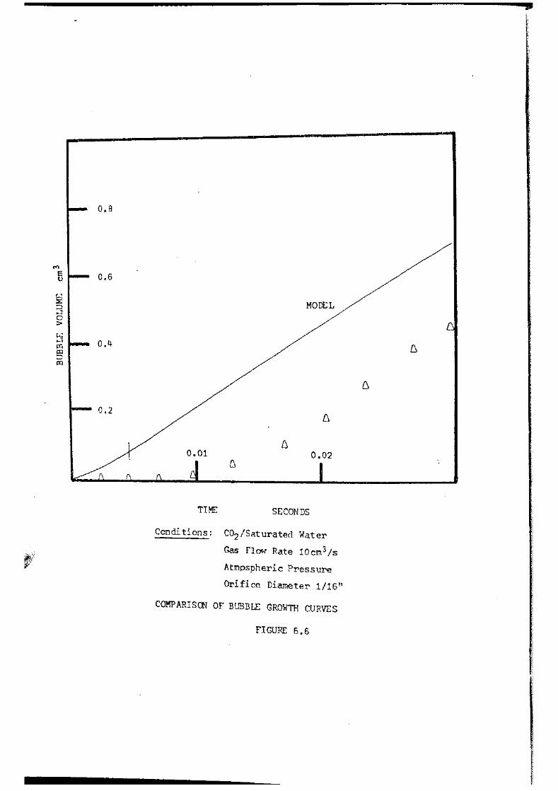
o.a
f'l')
E 0.6 l)
~ !::) ..:l 0 >
~ 0.4 J:Q ~ ~
;:;5
0.2
MODEL
0.02
TIME SECONDS
Conditions: C02/Saturated Water
Gas Flow Rate 10cm3/s
Atmospheric Pressure
Orifice Diameter 1/16"
COMPARISCN OF BUBBLE GROWTH CURVES
FIGURE 6.6
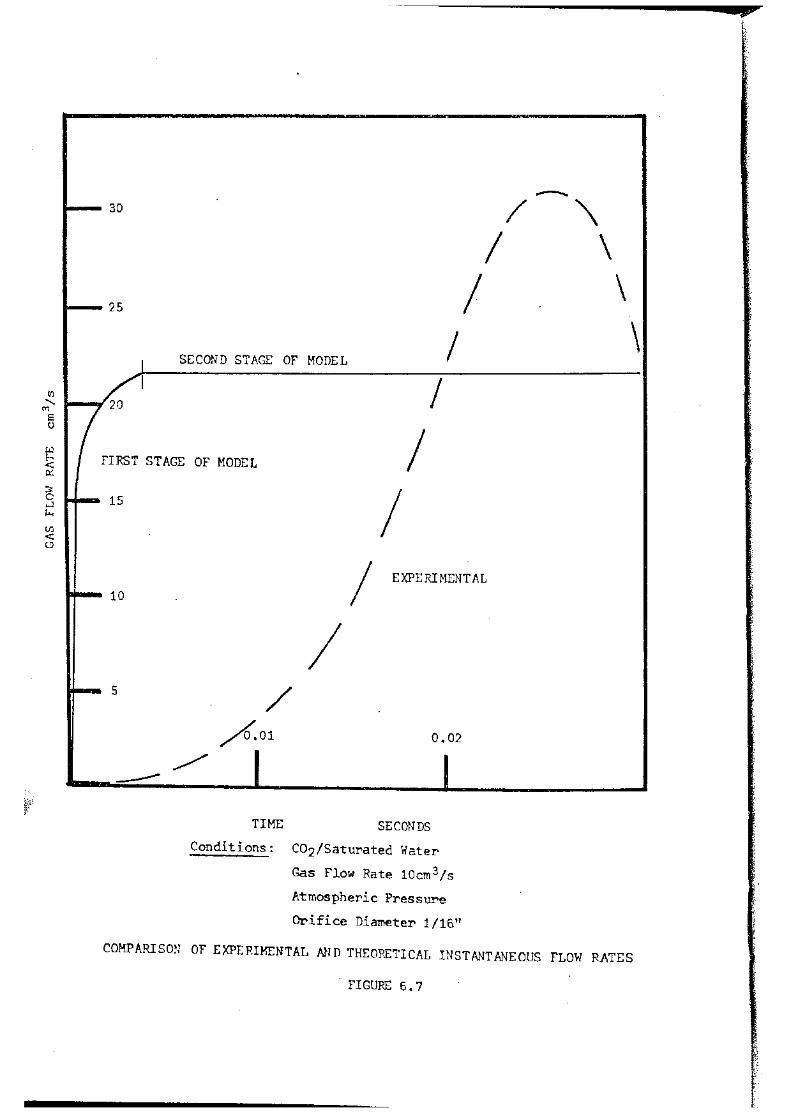
30
---25
SECOND STAGE OF MODEL
I I
/ I
FIRST STAGE OF MODEL
I
I
10
5
----
I I EXPERIMENTAL
I /
~01 0.02
TIME SECONDS
Conditions: C02/Saturated Water
Gas Flow Rate 10cm3/s
Atmospheric Pressure
Orifice Diameter 1/16"
\ \ \
\
COMPARISON OF EXPERIMENTAL MID THEOHETICAL INSTANTANEOUS FLO"t-1 RATES
FIGURE 6. 7

IJ.8.
examination of the floH equation is therefore justified. In thts section
the discussion is limited to a comparj_son of the instantaneous flow rate
computed from the flow equation and the theoretical grm·rth curve with
the experimental results. Alterations to the flow equation vrill be
suggested and discussed in section 8.5
Figures 6 .(-) and 6.1 shovr theoretical growth time and flow-time
curves obtained from an incremental solution of the flmv equation vri th
time for a flmv rate of 10 cm 3 /s at atmospheric pressure. The end of
each stage is computed from the usual force balances. The experimental
instantaneous flovr rates shovrn were obtained from differentiating a
least mean squares fit of the instantaneous volumes~ measured from the
photographic record in the manner discussed in Appendix 2.
It is evident from these Figures that even at atmospheric pressure
the model does not simulate the growth or flow into the forming bu.hble
vrith any accuracy.
r.rhree important features are noted:-
( 1) 'l,he experimental results indicate that during the initial
stage of formation the bubble grows slow·ly. Presumably
this is caused by the bubble having to overcome the inertia
of the liquid surrounding the orifice .. The model on the
other hand predicts a very :rapid increase in flovr rate
during this stage.
(2) The experimental results indicate that no constant flow
period exists at atmospheric pressure. The model predicts
a constant flo'\·7 rate for the greater part of formation.
( 3) The experimentally determined flow rate decreases as the
bubble accelerates a1vay from the orifice immediately prior
to detachment.
The model assumes that the flovr rate during the second stage
is constant. From the flow equation,

3.2
it is evident that this simplification 1dll become of increasing validity
as the pressure drop across the orifice, P1, increases. A large P1 vrill
mask the influence of the variable radial terms in the equation. This
is the case for high mass flo1-l rates.
Figure 6.7 shows that the first stage termination point is
reached so rapidly that the model might vrell be considered one of
"constant flovr" rather than "constant pressure''.
Collins (28) has adapted Davidson and Schulerrs constant flow
model (11) for increased gas momentum. The expression presented (28)
for the volume at detachment is,
For comparison the solution of this equation is plotted on Figures 6.1
to 6. 3. ~"'he adapted model approaches that of the constant flmv model
at high flo1v rates and increased system pressure as would be expected,
since for these conditions the adapted model predicts a very short first
growth stage.
The experimental results hovrever show· that there is no justi-
fication for this simplification. In particular the flow equation is
not an adequate representation of the flow into the bubble.
6.5 Discussion of the Model
It has been shown that there are significant differences bet.-vreen
the predictions of the model and the experimental findings. These diff-
erences are caused by fundamental inadequacies in the structure of the
model.
It vrould appear that useful progress depends on developing
a model which describes the continuous growth of the bubble using a
-~----

50.
more rigorous analysis than Kumar and co-worl~ers, \vhile accepting that
this will increase the computational procedure.
Refore discarding Kumar's model it is instructive to test the
sensitivity of the model to changes in experimental pa.rruneters, partie-
ularly pressure drop and orifice coefficient. This analysis will give
some indication of the accuracy required in me8.suring these system
variables if the computed volume is to have any worthi-Thile meaning.
§_~ .1 The Pressure D:r.S?1) Across the Orifice
The pressure drop across the orifice -vras measured ivi th a
manometer for the initial study 1-nrt later vri th a more sensitive pres sure
transducer. The mean pressure drop measured is small, of the order of
0.01 to 0.05 psi. An error of around ±10% could be expected in this
reading. This error causes a change in the predicted terminal volume
of ±5%. For example, the experimental pressure drop at atmospheric
pressure for a flovr rate of lOcm 3/ s is given belo1·r, together 1-Ti th the
results from a ±10% change in the pressure drop.
For 10 cm3 /s, 11 6 in. orifice at atmospheric pressure,
Pressure drop across the orifice (psi)
0.040 0.044 0.036
Predicted volume (cm3 )
0.48
0.50
0.46
6.5.2 The Orifice Coefficient
The orifice coefficient was taken as the same as that with
no liquid above the orifice. BcCann (19) notes from analysis of previous
investigations (25) that this value is likely to have a maximum error of
15%. It "ioTas found that such an error 1-rould cause a corresponding chane;e.
in final bubble volume of ±10%. For the same case given above the com-
puter results are,

Pressure drop across the orifice (psi)
o. ol~o o. ol~o 0.040
Orifice coefficient (em~ I e;m~)
0. 02l!f
0.0238
0.0190
51.
Predicted volume (em 3 )
o.~-8
0.53
0.45
The cumulative error from these parameters could result in a
15~~ chanc;e in the final volume. Figures 6.1 to 6. 3 shm·r that the average
error in the predictions is significantly greater. Increasing the
accuracy of measurement of these parameters above will not appreciably
decrease the deviation between model and experiment, emphasizing again
the more basic inadequacies in the mathematical formulation that have
already become apparent in section 6.4.3.
6.2.3 Gas Chamber Pressure
Constant pressure in the gas chamber \-ras assumed as a. simpli-
fication for the model. As indicated in section 6.4.3 the gas chamber
pressure did in fact vary. The pressure fluctuations in the gas chamber
will have a considerable influence on the flow into the bubble. Ex-·
press ions for this variation have been Cl.eveloped ( 19) ( 20) ~ but cannot be
included in this type of "mean" force balance model. An incremental
approach is needed if allowancie is to be made for the variation in
chamber pressure.
6.2.4 Other Factors
The problems of sphericity of the bubbles~ bubble interaction
and liquid circulation are common to all theoretical models. These will
be discussed in Chapter 12 when the model developed in Chapters 8 and 9
is considered.
6.6 Conclusions
The interpretation of the experimental results based on the
-guidelines developed in the previous chapter has led to a better under-
...........

52.
standing of the type of process occurring \·Ti th increased system pressure.
Gas density has a considerable influence on the formation
process at increased system pressu:res. For the same flmv rate; the
formation process l·ri th increased gas density becomes progressively more
complex, finally becoming chain bubbling at hie;h system pressures in
vrhich a great deal of interaction and coalescence occurs.
The predicted bubble volumes from the model adapted to include
the gas momentum and density, appear to follm·r the trend of the experi-
mental results.
A closer examination of the predictions of the growth rate
indicates that there is a need to develop a more accurate simulation
of the bubblin~ process even at atmospheric pressure. In particular,
an incremental approach with a more accurate prediction of the flow into
the bubble should be developed.
6.7 Recommendations from the Initial Stud~
(1) Experimental
(a) Further work is required to extend the range of
system variables studied.
(b) Investie;ation has sho-vm that accurate pressure measure
ments across the orifice are reQuired. Further vrork
should include a study on the variation of pressure
across the orifice.
( ) T ·b·l•t f It • "f d Tf • i " c he possJ. 1 1 y o a maxlmUm requency an a m.J..n mum
bubble size obtainable with increasing pressure should
be investigated.
(2) Theoretical
(a) A fundamental reap:praisal of bubble formation models
should be made.

53.
(b) rrhe equation to descr:i.be the flo1·T into the bubble shouJ.d
be altered to include inertial effects of the liquid
surrounding the orifice.
(c) Allm·rance for the variation of gas chamber pressure
should be included in any ne1·r model.

54.
AN APPHOACH ~:eo M:ODELLING GAS BUBBLE FORMi\.rriOH
7.1 Introduction
This chapter develops an approach to modelling gas bubble
formation at a single submerged orifice. The model of Kumar and co-
workers (15) (31), which ivas adapted in Chapter 3, is compared against
this approach.
7.2 An Idealised Picture of Formation
The flow of e;as through a submerged orifice under normal
circumstances results in the formation of discrete bubbles of similar
size. To properly analyse this process it is necessary to model the
interaction between the forces governing the growth from initiation
to detachment.
It has been established (5)(11)(14)(15) that the important
parameters determining the growth are liquicl inertia, viscous drag,
surface tension, hydrostatic head and the pressure drop across the
orifice.
In general the initiation of the formation period has been
taken as that instant vhen the bubble forms a hemisphere whose diameter
is equal to that of the orifice. It has been shown experimentally
that the grow·th normally proceeds from this point 1vi th continuous addi-
tion of gas until the bubble detaches, Figure 6.7.
In formulating an analytical solution there are two motions
of the gas-liquid interface to be considered. These are a radial
expansion resulting from the addition of mass to the bubble and a
vertical translation to ?-Ccommodate the restriction of the orifice
plate and the imbalance of forces on the interface. '1"11e two motions

are inseparable since any radial expansion will alt.e:r the vertical
translation~
55.
The expansion of the bubble requires work to be done by the
gas against the liquid. Thus from the outset the burJble must accelerate
from rest and a resultant upward force be maintained for continued gro~~h.
7.3 An Analytical Solution
An analytical solution for the motion of the forming bubble
requires the simultaneous solution of the equations which describe the
radial and vertical motions.
Since the bubble is growing and vork. must be done against the
interface it is reasonable to suppose that this situation may be adequately
described by an equation of motion and an energy equation.
The approach of Davidson and Schuler ( 11) ( 12) has been to
describe the vertical translation in terms of an equation of motion while
the radial components eminate from an orifice equation. The orifice
equation is a modification of Bernoulli's energy equation vrhich allows
for the work done in increasing the surface area as the gas flows into
the bubble. It is basically this approach that will be used. in the
incremental model developed here.
7.4 The Growth of the Bubble
The idealised picture now proposed is that the gro1~h of the
bubble occurs in one continuous stage from initiation to detachment. It
also requires that there exists throughout the growth period a continual
resultant upward force without which flow into the bubble from the chamber
below the orifice could not occur.
Davidson and Schuler (11)(12), amongst others (14)(19)(41),
describe the motion of the centre of the bubble as,
Buoyancy = Inertia 7.1

56.
The modified orifice equation has been exrJressed as a force
balance by Potter (65), viz,
Static Pressure Force
Surface Tension Force
Force due to pressure loss across the orifice
= Inertia of liquid
These ti.ro equations may be solved incrementally for the
radial and vertical components enabling gro-v1th to be modelled contin-
uously throughout formation.
If the initial conditions are taken as a radius equal to the
orifice radius and the centre of the bubble in the plane of the orifice,
then lift-off of the bubble occurs without discontinuity as a natural
consequence of the growth and rise of the bubble. Lift-off is
defined as that point at which the distance of the centre of the bubble
above the orifice becomes greater than the bubble radius.
Kumar and co-workers (15)(31) commence similarly~ developing
an equation of motion and of gas flow. Ho-vrever continuous application
of both equations is not undertaken. Separation of the formation process
into two stages together with certain assumptions enables the equations
to be solved independently.
These assumptions are:-
(i) That the buoyancy force equals the downward forces at and
only at the end of the first stage.
(ii) The end of the first stage co-incides with lift-off of the
bubble.
{iii) As a consequence of assumptions (i) and (ii) the equation
of motion and the modified orifice equation may be solved
simultaneously to obtain the volume of the bubble at lift-off.

DAVIDSON AND SCHULER ( 12)
· ooO OQ ~ - --·· !! __ o
INITIATION DETACP.MENT ---CONTINUOUS----
Equations
(1) Sum of Force = Inertia
(2) Flow Rate, Equation 3.2
Solution:
Simultaneous incremental solution
for volume with time.
tetachment:
Occurs when S = a + a0 , experi
mental justification
Lift-off
No particular significance
Initial Conditions
At t = o, a= o, s = o, a= o,
s = o.
KUMAR AND CO-HORKERS ( 15)
-~-Q_· nE
EXPANSION DETACHMENT
STAGE
(A)
DISCONTINUOUS
(1A) Sum of force = zero
STAGE
(B)
(2A) Flow Rate. Equation 3.2
(1B) Sum of force = Inertia
(2B) Flow rate = Constant
Stage A:
End of this stage occurs when
I:r = o, substitution for this
into flow equation, solve for
volume.
Stage B:
Analytical solution of equation
of motion, Q = const.
occurs when S = a+ ~, ~radius
at end of stage A, no justificat
ion.
Significant. This marks the end
of the expansion stage.
Conditions at t = o not specified.
Time eliminated from solution.
COMPARISON OF BUBBLE FORMATION MODELS
TABIE 7.1

Lift-off is followed 'by a rise periocl while the bubble expands but
is still attached to the orifice by a neck.
57.
( i v) During this ])eri od there is f'lm.;r into the bubble at a
constant rate determined by the orifice equation at lift-off.
(v) Termination occurs when the bubble has risen an arbitrarily
defined distance above the orifice.
7.5 Discussion of Kumar's Model
Having outlined an alternative approach to modelling bubble
:formation the discussion no"iv returns to KtUnar' s model for critical
comparison. The previous section has pointed out the differences
between the two approaches in the method of solution of the same basic
equations. Table 7 .1 compares the proposed approach based on Davidson
and Schuler' s work ( 11) ( 12 ) against that of Ku.m..~r and. co-workers ( 15) ~
7_. 5.1 Lift-off and the Force Balance in Kumar's Model
Assumption (i) ignores the fact that the centre of the bubble
about which the force balance applies is moving up1vard before and after
the liftg-off point, indicating a continual resultant upward force on
the bubble.
In the gro1~h of the bubble the only significance of the point
at vthich the bubble leaves the orifice is that the geometric restrictions
imposed by the orifice plate on bubble gro1rth are no longer limiting.
Equation 7. 3 below, is used by Kumar and co-workers to in
dicate the point at which the bubble lifts off the orifice.
Buoyancy = Inertia + Surface Tension + Viscous Drag 7.3
No justification is given by Kumar and co-workers (15) ( 31), nor can
any be found, for designating this equation as defining the point at
which the bubble lifts off. It is not valid merely to propose a plausible

58.
force balance and suggest that it describes one particular point in
the gro1·rth without further justification.
Further examination of equation 7.3 shows that the inertia
has been included in what -v1as termed a static force balance. Re·-
arranging this equation indicates that the authors are suggesting that
the equation to describe lift-off is,
Buoyancy - Surface Tension Viscous Drag = Inertia 7.4
This is a feasible equation of motion of the bubble. But if equation
7.4 is used to describe the motion of the bubble, it is easily shown
that the surface tension term, 1rd0 cr, used by Kumar and co-workers is
incorrect. At a point just after initiation (t=o, a~a0 ), the equation
of motion becomes,
= Inertia
+ where 0 indicates a positive quantity much smaller than the value of
1Td.0
cr. A continuous solution of equation 7. 4 would initiate the motion
of the bubble in a negative direction.
There are forces arising from the contact around the edge of
the orifice 1-Thich restrain the bubble from leaving the orifice. The
forces involved, however, are not those given by the static surface
tension. ~~e dynamic surface tension will be different (5)(66) and the
effect on the bubble growth is small (11) and can be ignored.
The surface tension, on the other hand, has an appreciable
effect on the energy required to Inaintain the interface. It will thus
affect the flmv into the bubble.
7.5.2 Detachment of the Bubble
The development of a criterion for detachment of the bubble
requires analysis of the gas-liquid interface of the neck taking into

DETACHMENT
Conditions: Atmospheric Pressure
002/Saturated Water
FIGURE 7.1 Orifice Diameter 1/16"
Liquid Seal 2"
FORMATION SEQUENCE SHOWING DETACHMENT TAKING PLACE AT A
DISTANCE APPROXIMATELY EQUAL TO THE ORIFICE RADIUS

Conditions: C~/Saturated Water
Gas Flow Rate 10cm3/s
Atmospheric Pressure
Orifice Diameter 1/16"
Detachment at:-
V 1 me = 0.825 cm 3 aE·, o u
a , 0
Volume = 0.480 cm 3
PREDICTED TERHINAL VOLUMES USING KUMAR'S MODEL (15) WITH DIFFEFENT
DETACHMENT CONDITIONS
FIGURE 7.2

59.
account the unsteady interaction of all the forces. Such analysis is
beyond the scope of this i·rork, but the literature indicates it is more
complex than that used by Kumar and co-workers.
The approach of previous investigators ( 5) ( 11) ( 19) ( 20) has
been to arbitrarily select or experimentally determine the distance
above the orifice at -vrhich detachment occurs. This has been found
experimentally to lie between a distance equal to the orifice radius
and the orifice diameter depending on the actual dimensions and flow
rate (20).
Kumar's model assumes that detachment occurs when the base
of the bu.bble has moved a distance equal to the radius at lift-off, a.E.
The value of a.E depends on the definition of lift-off, for which no
theoretical justification exists. Hence it must be concluded that this
criterion also has no analytical basis.
Kumar and co-vrorkers ( 31) go on to state that "this (distance)
nearly corresponds to the cond:i.tion l·rhere the rising bubble is not
caught up and coalesced (with) the next expanding bubble". If this
can be considered an experimental validation then it is in .. error since
the criterion sought is that distance at -vrhich a single bubble detaches
from the orifice not coalesces with the following bubble.
A typical series of photographs from this work sho\d.ng detach
ment taking place at a distance approximately equal to the orifice
radius are presented on Figure 7.1 For the same experimental conditions
Figure 7.2 shows the final volume using Kumar's criterion (cxE) and result
using cx 0 • The two solutions give quite different results. If the de
tachment is assumed to occur when the base of the bubble has moved a
distance above the orifice equal to the orifice radius, for which
there appears to be greater experimental justification~ then the model
no longer gives reasonable predictions.

60.
L 6 Conclusions
It has been the purpose of this chapter to develop a general
picture of an approach f'or modelling gas bubble formation at a sub
merged orifice.
An idealised picture of buhble formation suggested that the
gro\-rth of the bubble consisted of both a radial expansion and a vertical
translation. rrhe relative magnitude of these components depends on
the interaction of the forces on the bubbl.e. Since, both 1<rork must be
done against the interface and the bubble is in motion the growth may
be described by an equation of motion and an energy balance.
This picture was compared with the approach of Kumar and
co-workers (15) ( 31) ( 46) ( l+7).
The fundamental difference in their approach is the
adoption of an overall force balance. This retains simplicity by
dividing the bubble process into two distinct stages and applying a
static force balance to the end of the first stage and assuming constant
flow rate in the second.
The limitation of this approach is that transien~ effects,
which may have a considerable influence on the growth, are obscured.
A continuous incremental solution of the two basic equations could
provide this information.
~1e development of the model of Kumar and co-workers in this
work has been a \•TOrthwhile exercise since it has enabled an estimation
of the effect of gas momentum to be made without the mathematical
complexity which must inevitably result from the adoption of an incre
mental solution. However, this computational simplicity was achieved
at the expense of physical reality.

61.
CHAprl'ER 8
A MODEL FOR GAS BUJ3BLE FORMATION
1Vr ATMOSPHF!UC PTIESSURE
8.1 Slli!lmarr
A theoretical model for gas bubble formation applicable to
atmospheric conditions for a single submerged orifice under constant
pressure is derived, based on the continuous approach described j_n the
previ?us chapter. The model shows significant improvement over previous
models in predicting volume and gas flovr rates.
8.2 Introduction
Chapter 6 showed that Kumar's model adapted to allow for gas
mornentl.Ull masked important transient effects. Even at atmospheric
pressure the model did not follow the experimental gro\vth.
The previous chapter developed a general approach to a mathe-
matical solution for the gro-vrth of a forming bubble by describing the
radial and vertical components in terms of an equation of motion and
an energy equation for the expandins interface. This concept is developed
in quantitative terms, by extending the basic approach of Davidson and
Schuler (11)(12).
The success, of the model vrill depend on hovr accurately the
two simultaneous equations can be formulated. In this chapter deliberate
limits are placed on the variables in these equations by assuming
constant pressure conditions. This eliminates the effect of the gas
chamber and enables direct comparison with the models of Davidson and
Schuler (12) and Kumar and co-workers (15).
The interaction betiveen the bubble and the gas chamber pressures
is discussed in the next chapter.

~··'· jao I
t = 0 s = a
Initiation
FORMATION SEQUENCE FOR MODEL DEVELOPED IN
CHAPTER 8
FIGURE 8.1
me- -~~c
V/2>
s=a+a 0
Detachment

62.
8. 3 The 11ocJel and Its Ar;sumntions
1I'he model proposed follovrs the idealised picture of i'ormation
outlined in Section 7'. 2. Initially the bubble centre is at a point
source of gas, the centre of the upper face of the orifice, and its
upi-rard motion is determined by a balance bet1-reen buoyancy and inertia.
It is assumed that;
(1) Circulation of liquid is negligible.
(2) The motion of the bubble is not affected by the presence of
other bubbles.
(3) 'rhe virtual mass may be used to describe the inertia of
the liquid surrounding the bubble (11) •
( l~) Bubbling is taking place under constant pressure condi t1.ons.
(5) The drag on the bubble may be neglected. It has been argued
(12) that for low viscosity fluids the wake behind the
forming bubble is not fully developed until after detachment,
hence the flow around the forming bubble may be assumed
irrotational and unseparated. That is, the fluid may be
considered inviscid and the drag ignored.
(6) 'I'he bubble grmvs spherically. Davidson and Schuler (11)
assumed spherical grm.rth. This cannot be achieved experi
mentally as the base of the bubble is prevented from
moving do-vm-vrards by the orif:i.ce plate. The model here
considers only that spherical segment of the bubble which
is above the plane of the orifice.
The sequence of events on which the model is based is sho-vm
011 Figure 8 .1. The bub1)le expands and rises as the gas flows through
the orifice. Lift-off occurs as a result of this process. After lift-off
the gas is supplied to the bubble through a neck until the base has risen
an experimentally determined average distance.
sd

63.
8. ).~ Th!; Eguation of Hotion
The upward motion of the bubble is determined by the buoyancy
which results in the mass acceleration of the liquid surrounding the
forming bubble. That is,
V(p- p')g = Buoyancy
d(HS_l dt
Inertia
8.1
where the effective inertia of the fluid surrounding the bubble is
assumed to be accounted for by taking the virtual mass of the bubble (ll).
In section 3.6.2 it was pointed out that the term used for the
virtual mass, (p' + ~)V, applies only to a completely inviscid liquid
where the bubble is moving perpendicular to a wall (11) (55), here the
orifice plate. It has been argued ho-vrever, (19) that the virtual mass
in this case could take on a value from (p' + ~p)V to (p' + p)V. If
the motion of the bubble was considered to be that of a bubble moving
parallel to a wall, say the vessel wall or the orifice, then a value
greater than (p'+ p)V could be derived (67). Generally the value
( p 1 + ~ )V has been taken as giving reasonable agreement with experi
mental results and will be used in this analysis ..
The equation of motion can thus be expanded to,
11 . v(p- p')g= (p' +w)(vs +vs) 8.2
8.5 The Energy Equation
Davidson and Schuler (11) assume that an orifice equation of
the form Q = k~P~ can be modified to give the flow into the bubble.
Q = V = K (Pl - ngh + pgs -20 )~ (p' )~ ~ a 3.2
The importance of this equation in determining the final bubble volume
was demonstrated in Chapter 6. It -vrill now be examined in greater detail.
---

64.
Potter ( 65) has sho\vn ho-vr the ori i'ice equation can be derived
from a force balance over the liquid column from the orifice to the
free liquid surface.
This can be expressed as,
Sum of Forces = Inertial Terms
Davidson and Schuler (11) assume that the inertial terms are
zero, arriving at,
8.3
This is based on calculation of the kinetic energy imparted to the
liquid surrounding the bubble by the radial motion. They conclude that
it is negligibJ_e in comparison with the other forces involved. The
expression, QP Bnat , (11) for the mean pressure that must be applied to
the bubble interface to overcome the inertia caused by radial motion
has large values during the early stage of formation when both a and t
are small.
The effect of the radial acceleration of the liquid surrounding
the forming bubble has also been dete1~ined by Kupferberg and Jameson (20)
:from consideration of the potential flow around the bubble. They find
that it has an important effect on the grow-th of the bubble. The rele-
vant term is,
Although this strictly applies to the ~hole sphere it is assumed in
this analysis to be applicable to that portion of a sphere above the
orifice. The reaction of the orifice plate is neglected.
During the formation of the bubble there are two motions to
be considered, expansion and translation. The expression just given
refers to the radial acceleration of the liquid immediately surrotmding
---

the bubble. Potter ( 65) shm·rs that the e:ffect of the inertia due to
vertical translation of the forming bubble is of si~nificance when
compared \·Ti th the other forces acting. He represents this effect by
phV the term A but does not explore the consequences of using it in a
formation model.
Including these terms the final modified orifice equation
becomes:-
P 1 - pgh + pgs -
Static Hydro-pressure static drop loss
Pressure caused by surface tension
1 . 2 -2 (V) K
Pressure loss through the orifice
8.6 Solution of the Equations
8.4
+
Inertia Inertia of of liquid liquid surr-due to ounding the. translation bubble
The volume of the bubble and its derivatives may be expressed
as:-
for s <a for s > a
v = 'IT ( 2;3 a3 + a.2s -s~·) 3
v = ~3rra3
v = n(2a 2a + 2a.as + a 2ss - s 2s) v = lnra 2&
v = n(a(2a2 + 2as) + 2a2 (2a + s) v = 4n(2a&2 + a 2a) + 4aa.s - 2ss 2 + s(a2 - s2)
and !J.P 0
is obtained. by equating the. work done in expansion to the
increase in surface energy, 6PcrdV = crdA
whence 6P0 =
=
By taking,
and,
2cr(3a. + s)
a = x
. s = y
2cr a
for s <a 8.8.1
for s > a 8.8.2
8.9
8.10
8.5
8.6
8.7
-----

2 a 0 K
em em 112/ 1__.
gm"2
.298 1.9
.298 1.9
.298 1.9
• 3'71~ 3.06
• 371~ 3.06
.37h 3.06
.~12 3.82
.~12 3.82
.412 3.82
.460 4.9
.460 4.9
.460 4.9
.460 4.9
Table 8.1
Formation of air bubbles in water with constant pressure a = 72 dyn/cm
2cr I af !'1f'~AN GAS FLOW nATE, Q BUBBLE VOLUME, V p
g/cm dyn- EXP'I' • RF. F. REF. 'J'his Work EXP'I': REF. RFF. This Work oec2 cm2 (12) (15) h=5 h=lO h=l5 (12) (15) h=~ h=lO h==l5
951* 968 32 G7 65.5 h4.4 4240 40.6 2.3 3.5 3.29 3.06 2.95 2.83
1118 968 45 70 68.0 51.6 50.3 )~9. 0 2.9 3.8 3.52 3.55 3.46 3.42
1323 968 61 76 73.2 58.9 57.5 56.2 3.4 4.2 3.78 4.02 3.95 3.B9
779 771 33 102 86.4 63.6 59.4 56.9 3.2 6.1 5.89 4.88 4.59 4.31
877 771 47 105 89.7 73.2 68.8 66.2 4.1 6.4 6.13 5.54 5.32 5.07
1024 771 6o 112 93·9 83.8 79.2 76.h 4.5 6.9 6. 4·r 6.26 6.09 5.78
734 698 30 124 109.0 80.9 73.4 69.9 4.3 7.8 7.88 6.37 5.85 5. !~ 3
832 698 57 129 113.0 89.3 85.4 79.8 4.9 8.3 8.18 7.16 6.71 6 '?7 • ...) I I
1006 698 68 1}+1 118.2 10l1. 0 99.7 93.7 5.7 9.1 7.98 8.25 7.86 7. 5li '
6~2 625 25 156 135.0 93.1 83.4 73.6 5.6 10.7 10.73 7.78 6.93 5.80
739 625 6o 163 14Q.5 110.0 99.4 91.6 6.9 11.4 11.18 9.10 8.29 7.45
790 625 68 169 142.8 113.0 lOT.O 97.2 7.1 11.7 11.39 9.60 8.85 8.09
800 625 170 169 - 114.0 108.0 101.0 7.5 11.8 - 9.69 8.95 8.34
*This case represents the minimum volume and flow rate predicted by the model as P+;a see ref. (12) 0

66.
the equation of m.otion 8. 3 ca.n be rearranged to gi 1re,
y = fl(a., s, x, y) 8.11
and rearrangement of equation 8. 4 and substitution of the expressions
for the volume and its derivatives,together with equation 8.11 leads
to,
x = f'2(a, s, x, y) 8.12
These four first order differential equations (equations 8.9
to 8.12) have been solved simultaneously for a, s, x andy using a
:fourth order Runge-Kutta (Gill modification) numerical technique for the
initial conditions at t = 0 of a= a. 0 , s = O, x = 0, y = 0. The detach-
ment criterion was taken as s = a + a to allow for the initial volume 0
No theoretical justification of this detachment criterjon has
been made in this ftnalysi s. Instead the instant of detachment has been
observed experimentally (for example, Figure 7.1) and found to be of
this order.
The solution and computer prograoone for these equations is
given in Appendix 4.
8.7 Results and Discussion
Table 8.1 compares the predictions of the model with those
of Davidson and Schuler ( 12) and Kumar and co-workers ( 15) for the
experimental study of Davidson and Schuler (12). The theoretical values
of the mean flow rate Q and the final volume VF have been greatly reduced
f'rom those previously reported, by the inclusion· of the terms for the
acceleration of the liquid and the more stringent geometric represent-
ation. The results from these modifications are significantly closer
to the experimental values~ particularly for the larger diameter orifices.
-

a: tl
[j ~ ~ U) H t=l
1.2
1.0
o.a
0.6
0.4
0.03 0.04 o.os 0.06
TIME SECONDS
Theoretical curves for radius, a (em) and distance from
orifice, s (em) with time for the case a : 0,167 (em) 0
P = 877 (gm/cm sec2 ) h = 10 (em).
FIGURE 8.2
~
CY. 0
0.07

N (.)
<ll (./)
s 6.0 tl
' Sc ('oJ 0 ,..;
X s.o <( H
t; ~1 ........ H
Q
~ 80 0 4.0 H .....:1 n
3 w
........ til
3.0 60
LIQUID
INERTIA v v
(1)
s tJ
~ 40 f;:.."' .... H 0 > -~
1-1
P4 §!
20 &:CI 1.0
TIHE SECONDS
Theoretical curves for bubble volume, V (cm3), instantaneous .. ' ' • 3 ph~~+ p (,..:: + 3/2(~)2) flow rate, V (em /sec) and liquid inertia uu ~
A for the case a 0 0.167 (em) P = 877 (gm/cm sec2 ) h = 10 (em).
FIGURE 8. 3

(',/ ()
<l.l ttl
t1 6.0
' ~ ('I bt
(
(',/
0 ,-I
oil .. X s.o E < ~ H :;:: ~ 1-
t,..:; (::. z t: H
c A .. _ H ~ ::::;
80 Cl 4.0 H ...:l (')
:1 w
........ (I)
3.0 60
LIQUID ("•) v v E INERTIA (.)
('1
~ F--.- (.) :=: __, ..:I c...:: o, ~ > .......,
.,..:)
·~ 0 >
I=Q
g] :-3 p:) I=Q
f§ CQ 1.0
TIME SECONDS
Theoretical curves for bubble volume, V (cm 3), instantaneous .. · • 3 PhV + p ("':,: + 3 / 2 (~)2) flow rate, V (em /sec) and liquid inertia ~u ~
A for the case <10 0.167 (em) P = f377 ( gm/ em sec2 ) h = 10 (em).
FIGURE 8. 3

67.
In the original i·To:rk of Davidson and Schuler (12) the liquid
depth is not explicitly specified, being included in the pressure P.
However the liquid depths 1-rere beti·reen 5 and 15 em. Results are pre
sented for h = 5, 10 and 15 em. TaJdng the extremes of this range does
not alter the increased accuracy of the results to any great extent,
for instance, for the case P = 877 (gm/cm.s2) given in Figure 8.2 and
8.3, for h = 5,
for h = 15,
Vp = 5.54
Vp = 5.07
'Q" = 73.2
Q = 66.2
The plot of h.tb1)le growth, instantaneous f'low rate and accel
eration of the bubble, Figure 8. 3) shovrs that the acceleration of the
liquid column is most marked during the initial stages of formation '
at vrhich time it has a considerable influence on the flow into the bubble.
This is reflected in the growth and flow curves -vrhicb shovr the character
istic initial gro,..rth period found experimentally at atm pressure (cf. Fig
ure 6.6 and 6.7). Subsequently the acceleration of the liquid column
decreases rapidly, passes through a minimum and then rises to a smaller
maximum. The second maximum occurs for the time at which s = a. The
curve indicates t-vio periods in which the acceleration of the liquid surr
ounding the bubble is important. The two stage grovrth model (15) suggested
f'rom experimental evidence ( 27) may be explained by a single stage model
by the inclusion of the inertial terms in the orifice equation.
Before a qu.anti tati ve comparison between the model and the
experimental rt'3Sults of this study is made, the model vrill need adaption
to include variable gas chamber pressure and gas density.
8.8 Conclusion
1~e rate of growth of the bubble at any particular time is
dependent on the rela.ti ve magnitudes of the forces acting on the bubble
at that time. Comparison of theory and experiment based only on the

68.
final bubble volume did not allm-r the assessment of the instantaneous
forces,whereas the use of an incremental force balance approach gives the
magnitudes of these forces at each instant during formation.
rl1he effect of terms, such as the inertia terms, which have
a low mean value over the total formation period but a relatively large
effect at some stage of the grmnh -vrere obscured in the mean or final
force balance model (15) which predicted only final bubble volumes.
This approach -vrould be an undesirable simplification in certain circum
stances, for instance, in the study of mass transfer during bubble
formation where it would pe preferable to know the volume at all times.
For the experimental data of Davidson and Schuler (12)~ the
model presented shO\vS considerable improvement over previous models
(12) (15) in predicting bubble volume and mean gas flow rate over a wide
range of orifice radius and gas flow rate.
5

CHAP'I'EH q ___ ._., ........ -=-.
A t-10DI~.:._D~B_ GAS PU]iBL~.EQBJ~·lJ\~r~OJl_ \·TEICH INCLUDES V ~~LJ~
Q.~S CITJ~:_u~:ll._YR~SSUHE J\JTD GAS HOMENTUM
The model developed in Chapter 8 for constant chrunber pressure
and system pressure near atmospheric is no-vr adapted to include gas
momentum and variation of pressure in the gas chamber. Examples of
the predictions of the model showing the important parameters affecting
groi·rth are presented.
9. 2 The t1ornentum of the Gas
It vra.s shovrn in Chapter 3 that the increased gas o.ensi ty
encountered at higher system pressures requires the inclusion in the
model of a term for the momentum of the gas. Tbe expression used in
Chapter 3 describes the average rate of change of momentum over the
total formation period. The instantaneous rate of change of gas mo
p'V2 mentum, derived in Appendix 2, is given by Including this
expression into equation 8.2 gives,
pI (V) 2 v ( p - p I ) g + .:..,._.;_..;.,._ Ao
::: d(Ms) dt
Ao
= 11 . ..
(p' + 16P)(vs +Vs)
9. 3 rrhe Variation of Gas Chamber Pressure
9.1
The assumption of constant pressure behaviour eliminated
the interaction between the bubble and the gas chamber. A pressure
transducer across the orifice show·ed that cyclic pressure variations
were occurring similar to those observed by Kupferberg and Jameson (43).
A means of allo1-ring for this variation is developed below.
The capacitance of the gas chamber supplying the forming

70.
bubble is its a.bili ty to match the rate of supply of gas to the chamber
against that supplying the forming bubble. I'he variation of pressu.re
in the chamber may be found by assuming adiabatic behaviour of the
gas in the chamber ( 19) ( 20) .
For a chamber volume Vc, the pressure, p, at any instant
of time, t, may be expressed as (20),
p = 9.2
where c 0 is the speed of sound in the gas of density p'.
Equation 9.2 merely expresses that if there is a difference
between inflowing and outflowing gas rates there is a corresponding
pressure change.
The initial pressure pt=o, is that required to overcome
the resistance of the liquid meniscus,
Pt=o = Patm + pgh + 9.3
Equation 9.2 and 9.3 when substituted into the orifice
equation give,
rv -- v - Qt] L t=o
9.4
9. h The Lapse Period
The formation of a bubble at the orifice will lower the
· th h b r Depending on the capacity of the chamber pressure ~n · e gas c am e .
there 1vill be a lapse period after detaclnnent during which the pressure
in the chamber recovers to that required to initiate growth·
From equation 9.2 the pressure recovery can be expressed
as (20),

c 2pr p == Pt==tp + ....,..?_ Q.t
vc where Pt==t is the pressure of the ch.amber at detachment,
f
and by rearrangement the lapse period is given by,
t L 9.6
The frequency of formation is simply the reciprocal of the
total formation time.
f = 1 9.7
9.6 ~~e Flow Rate
'11te model computes the instantaneous flmv rate, V, into the
bubl.>le. ':Phe n.verage flow· rate into the bubble, Q, can be calculated
:from, tF
Jt . . Q Vdt E v !:.t
9.8 = a.. :::
tF t=o tF
'fhc overall mean flow rate, Q, however~ differs from the
averar;e flow rate into the bubble as it must allow for the lapse
period when no fJ.ovr occurs. The mean flow rate may be calculated
from the precl:i.ctecl voJ.ume and the total formation time.
9.7 The Solution of the Equations
'I'he procedure f'or the solution of the simultaneous equations
9 . l an . ~ 1 s e s a:me d 9 l · th as described in Chapter 8 and detailed in
Appendix 1~.
For the initial conditions, a= a0 ~ s = 0, x = 0, Y = 0
71.
-

-
('f")
g 0
~ ........ ..:I 0 >
~ P=l
~ P=l
0.8
0.6
0,4
0.2
MODEL
(CHAPTER 9)
(j
TIME SECONDS
Conditions: C02/Saturated Water
Gas Flow Rate 10cm 3/s
Atmospheric Pressure
Orifice Diameter 1/16"
COMPARISON OF EXPERil·1ENTAL GROWTH CURVE HITH PHEDICTIONS OF THE NEW MOnr:r,
FIGURE 9.1

t'i .......
C'l")
E (.)
w E-< < p::;
~ c ...::l
"'"' (.'j
< c
30
25
20
15
10
5
/'\
I \EXPERIMENTAL
I '
1 NO DEL I ( CH!'\PTER
I I
0.02 0.03 0.04
TD·IE SECONDS
Conditions= C02/Saturated Water
Gas Flow Rate 10cm 3/s
Atmospheric Pressure
Orifice Diameter 1/16"
9)
0.05
CO!PARISO!I OF EX?EPJ!l ti1AL ftJID Th'EORETICAL INSTANT.A.NEOUS FLOH RATES
. FIGUP-.E 9.2
--...... ____________ __

1-t <
~ :::> (/) en
~ ~
('i
c l: E-< u ...... ~ ~ H~ f-<'"0 <C ~,..,
~~ ~X ::>t,..{ c::: {.) CI.JH ~~ P:!:H ~0:::
0 p;; f..:!
~ < ::r: {.)
tf.l < t!)
-1
-2
SECONDS
~ I \ /DETACHMENT
v MODEL
I DETACHMENT
EXPERIMENTAL
Conditions:
INITIATION
C02/Saturated Water
Gas Flow Rate 10 em 3 /s
Atmospheric Pressure
Orifice Diameter 3/16"
GAS CHAMBER PRESSURE FLUCTUATIONS FOR SINGLE BUBBLE FOR!MTION
AT ATMOSPHERIC PRESSURE
FIGURE 9.3

72~
the :programme proc;ressively calculates a, s., x~ y, x~ y for inte:r:vals
of time. From these results the volume, frequency, flo1.r rates and
values of the various forces acting can be derived.
2. 8 Comnari"~_of the Moclel \·Ti th Exneriment at Atmospheric
Pressure
Figures 9 .l. and 9. 2 compare experimental gro-vrth and instan-
taneous flo1-1 rates at atmosr;heric pressure vri th the theoretical pre-
dictions :for the condi tiona against vrhich Kumar's model was previously
tested, Figure 6.6 and 6.7.
Closer agreement betveen theory and practice is obtained with
the present model. The inertial terms and the variable gas chamber
pressure give a more accurate simulation of the grcnvth, particularly
near the commencement. The improvement comes from adapting a more
realistic picture of formation although this results in a more complex
analytical solution.
The model predicts the initially slow increase in flow rate
and the maximum occurring experimentally. However the drop.in experi-
mental flow rate, which takes place towards the end of the formation
period as the neck stretches before detachment, is not predicte~ since
growth in the model is terminated when the base of the bubble reaches
an arbitrarily selected distance. The limitation is not serious, since
reasonable agreement has been obtained for the greater part of formation,
and variation in the first differentiru. V at the end of formation
effects V to a lesser extent.
Figure 9.3 illustrates the pressure fluctuations in the gas
chamber at atmospheric pressure for single bubble formation. The model
agrees with the experimental variation in both magnitude and frequency.
The eX-perimental curve indicates some instability possibly caused by
:fluctuation of the interface and swirl of gas in the chrunber.

'(3.
The expression used fo:r the variation of pressure has been
tested extensively at atmospheric pressure by Kupferberg and Jameson
(43) and McCann (19). Their investigations indicate that the model
closely follovrs the experimental results over a wide range of chamber
capacities.
The results presented in this section, together with the
comparison vri th Davidson and Schuler's ( 12) study, demonstrate that
at atmospheric pressure the model developed is a significant improvement
over previous models -vrhich have adopted the force balance approach ( 12)
(15). The following chapters use this moclel to predict bubble formation
with increased gas momentum.
9.9 Discussion of the Model
This section examines the sensitivity of the model predictions
to the experimentally determined constants and the variation of the
parameters governing the bubble growth. Detailed comparison of volume,
frequency and pressure fluctuations together with a discussion of the
limitations of the model is undertalcen in the next chapters.
The inclusion of the expression for gas chrunber pressure
eliminates the need to measure experimentally the pressure drop across
the orifice. This removes one of the sources of error inherent in the
model adopted in Chapter 3.
9.9.1 Sensitivity of the M6del to Changes in the
Orifice Coefficient
The orifice coefficient is the only constant vrhich must be
determined experimentally. It was shown that Kumar's model (section
6.5.2) was sensitive to variation in the value of the orifice coeffi-
cient.
Figure 9.4 demonstrates the effect on the predicted terminal

~ s (J
r£1
a 0 > ~-q ...:I ·,::q p:j
::::> ~
1.6
1.4
1.2
1.0.
o.B
0.6
5
K :: 0.04
K = 0.02
10 15 20
GAS FLOW RATE cm3/s
Parameter: Orifice Coef~icient, "·
Conditions: C02/Saturated Water.
Atmospheric Pressure.
Orifice Diameter • ~ 6".
Liquid Seal 2".
25
VARIATION OF PREDICTED BUBBLE VOLU~m WITH ORIFICIE COEFFICIENT
FIGURE o.L.

N 0 <l.l (/)
........
n s bO
N 0 .-i
~
~ ~ 0 ~
10
5
-5
DRY PLATE PPESSURE DROP
10
BUOYANCY
5
RATE OF CHANGE OF
GAS MOMENTUM
PRESSURE CAUSED BY
SURFACE TENSION
0.03 0.04 SECONDS
Conditions: C02/Saturated Water Gas Flow Rate 10crn3/s Atmospheric Pressure Orifice Diameter 1/16"
-10
-15
-20
C'J t) Q) tl.l
E ()
.......... f,: no
N 0 rl
X
~ ;::). (f.) (j)
~ P-l
P Pl (v.)2/K2 arameters: Dry ate Pressure Drop................ -Buoyancy •••••• •.• •.••••••••• , ••••••••••• V(p-p' )g Rate of Change of Gas Momentum ••••••••• p' ( V) 2 /A0 Head •••••••••••••••••• ~ ••••••••••• , •••• pgs Pressu~ Caused by Surface Tension ••••• ~Fa
VARIATION OF PARAMETERS EFFECTING BUBBLE GROW'l'H VERSUS TIME
FIGURE 9 .. 5

N 0 l""i
X
G) ()
J..c 0
J%.
!<1-:'im---------,
Dry Plate Pressure Drop
15
10
5 5
-5
-10
Parameters: Dry Plate Pressure Drop •••••••••• Buoyancy ••••••••••••••••••••••• Rate of Change of Gas Momentum ••• Head • • • • • • • • • • • pgs Pressure Caused by Surface Tension APcr
Conditions: C02 / Saturated Water Gas Flow Rate 10 cm3/s System Pressure 250 psig. Orifice Dia.'neter ~ 6 "
VA.~IATIO!l OF P~W·1ETERS EFFECTING BUBBLE GROvJTH VERSUS TIME
FIGURE 9.6 ·-------

---
Parameter: System Pressure
·Conditions: C02/Saturated Water
Gas Flow Rate 10 cm 3/s
Orifice Diameter 1/16"
PREDICTED VARIATION OF INERTIAL TERMS, ( £'22Y + p(a~ + 3/2(~)2)) ~ A
WITH TIME
FIGURE 9. 7

N ().
~ tf.)
...... s u
100
0.04
TIME SECONDS
Parameter: System Pressure
Conditions: C02/Saturated Water
Gas Flow Rate 20 cm3/s
Orifice Diameter 1/16,.
0
PREDICTED VARIATION OF RATE OF CHANGE OF GAS MOMENTUM WITH TIME
FIGURE 9. 8

volume of altering the orifice coefficient. The model sho-vrs a similar
sensitivity to that of the mode1 e.dapted from Kumar and co-workers (15).
It is therefore of cons:Ldera1)le importance that the orifice
coefficient is measured aceurately. It would be possible to predict
the coef'fic ient from equn.t ions, such as that by McAllister ( 68), but
these are themselves sub.j ect to error and usually apply to standard
ori:fice dimensions. ':Phe value of the orifice coefficient thus remains
the most critical experimental parameter.
9. 9. 2 Pararncj;~:.:r.s Affec_!J..pr; Growth
Figures 9. 5 and 9. 6 sho,·r the predicted variation with time
o:f the parameters influencing the gro'\-rth of the bubble at atmospheric
pressure and 250 psig. respectively.
The diat:;rruns shovr that initially the s'LU"'face tension and
liquid inertia have the ET,reatest influence on bubble growth. As the
bubble becomes larger the hydrostatic head, pressure drop a-cross the
orifice and the buoyancy dominate.
Figure 9. 7 and 9. 8 comparE~ the inertial terms e.nd rate of
change of gas momenttun for different pressm~es. The graphs shovr that
the liquid inertia is more marked. at increased. pressure. This however
is compensated for by the increased influence of gas density on the
momentum.
9 .J.O __ .~on~~~Jon_§_
The previous three chapters have developed from basic principles
a sinele stage model to overcom·2 the inadelrw.cies existing in a tw·o
stage model. The model proposed has the following features:-
( l) It is incremental and models the grovrth of the bubble
from initiation to detachment.
(2) It makes allow·ance for variable gas chamber })ressure.
-

75.
(3) It accounts for the effect of the inertia of the liquid
surrounding the bubble.
( 4) It a.llo"l..rs for the momentum of the gas.
The model, tested thus far at atmospheric pressure, shows
improvement in predicting terminal volume and flow rates over similar
approaches.

A. A'IMOSPHERIC PRESSURE
B. 150 psig
C. 300 psig
Condi tiona: C~/Saturated Water
Orifice Diameter 1/8"
Liquid Seal 2"
GAS BUBBLE BEHAVIOUR FOR A CONSTANT VOLUMETRIC FLOW-RATE OF 10cm3/s AT SYSTE~ CONDITIONS
FIGURE 10.1

A. ATMOSPHERIC PRESSURE
B. 150 psig
c. 300 psig
Ccmdi tions: C<>2/Saturated Water
Orifice Diameter 3/16" Liquid Seal 2"
GAS BUBBLE BEHAVIOUR FOR CONSTANT VOLUMETRIC FLOW-RATE OF 10cm3/s AT SYSTEM CONDITIONS
FIGURE 10.2
1

76.
QJJANTI1:'~rriVE CO!~iPA:R J.~;cm OF E'lPER ]}!ENTAL RESUirCS -------,-··-~-----~ ---
HITH HODF:L T'IyJ)ICTIONS l'{fl__ INCHRAf1ED PRESSURE
10.1 Introduction _______ ,..._tl~,... .. - ____ _
This chapter details experimental data for terminal volume,
frequency, "bubble growth and pressure fluctuations for a wide range of
system pressures and flow rates. The predictions of the proposed forma-
tion model are tested against this data. The results show that the new
model presents a more realistic picture of formation with increased gas
momentum than the moc1el adapted from Kumar and co-vrorkeJ:•s ( 15) .
10.2 Ex:re:r-:I.mental Procedure
The apJ)ar.atus used in the ini.tial study wa_s modified to include
a f'a.st res1)onse r>ressure transducer placed across the orifice. The experi-
mental procedure i.s given i.n Chapter 2, calculation is based on the inter-
preta.tion of the photographs outlined in Chapter 5.
10. 3 Ran£:~ of Experimental Conditions Studiec;_
r:J~he stud.y covers the follo1-ring experimental conditions:-
(1) 1;16
1/8 31 6 inch diameter orifices (see· section 2.2).
( 2) 0 to 300 psig system pressure.
(3) 1 to 30 cm3/s flow rate C02 at system conditions.
( !1.) 2 to 6 inch water depth above the orifice.
(5) All runs were made at room temperature (18 to 22°C)
10.4 Results and Discussion
The results will be analysed in six main sections,
( i) Bubble VoJ_wne
(ii) Bubble Frequency

(iii) Bubble Grovrth
(iv) Flow Rate
(v) Bubbling Regimes
(vi) Pressure Variation in the Gas Chamber
10. l+ .1 General Behaviour - Effect of Orifice Size
T·r.
Figure 10.1 and 10.2 illustrate carbon-dioxide bubbling through
the 1_,.g and 3/16 inch diameter orifices into water at a constant flow rate
of 10 cm3 /s over the range of pressures studied. 'l'he formation behaviour
shown may be compared with Figure 4.2 for the 11 6inch orifice.
For the two larger orifices the formation process remains
simpler at high pressures than observed for the same flow rate through
the 1;]_ 6 inch orifice. Although chaining occurs at 300 psig for the
larger orifices, the degree of interaction and coalescence is less than
with the 11 6 inch orifice. Some simplification is expected since the
corresponding gas velocity through the orifice is reduced.
10.4.2 Bubble Volume
(1) The Effect of Flow Rate at Fixed System Pressure
Figure 10.3 and 10.4 illustrate the experimental volumes versus
:flow ra.te for different system pressures. At atmospheric pressure the
vollrrne increases linearly with flow rate, this indicates a constant bubble
:freQuency (15)(19). The results at pressures above atmospheric do not
sho\or this linear dependence throughout the range of flow rates. Both
volume and freQuency increase simultaneously to accommodate the increase
in flow rate.
The effect of orifice size on bubble volume for a constant gas
velocity of 200 cm/s through the orifice is shown in Figure 10.5. The
bubble size increases with orifice diameter although the influence of
orifice size is less signi.ficant as the system pressure increases.

t'l")
0 ~ ~ ...:! 0 >
~ (!I
§ (!I
-
I <>
<> 0 PSIG [::::J 50 PSIG 0 100 PSIG
1.4 ~ 150 PSIG
0 300 PSIG 0
<> 1.2
I 1.0 0
<>
I ~ 0.8 <> C::.l
I / <>¢ C::J
/ ~ <> 0.6 ~ ~0 I y
0 ~--------<> <>
/ ----~ ,0----I
0
/ 00/ ~% ifJ ~~
~/~ 0.2[;::) ~ 0
{%~ ~ 5 10 15 20
GAS FLOW RATE cm3/s
Parameter: System Pressure
Conditions: C02/Saturated Water
Orifice Diameter 1/8"
Liquid· Seal 2"
EXPERIMENTAL BUBBLE VOLUME VERSUS GAS FLOW RATE
FIGURE 10.3
25
o·

1.4
1.2
1.0
0.8
0.6
0 0 PSIG
~ 50 PSIG 0 100 PSIG
~ 150 PSIG
0 300 PSIG
5 10 15 20
GAS FLOW RATE cm 3/s
Parameter: System Pressure
Conditions: C02/Saturated Water
Orifice Diameter 3/16"
Liquid Seal 2" .
<j
I /
t::J
/
. 25
EXPERIMENTAL BUBBLE VOLUME VERSUS GAS FLO~T RATE
FIGURE 10.4

("f")
s u c..-1 ::8 ::> ...:I 0 > w t-.:1 ,:Q
g3 lXI
1/16
1.0
0.8
0
0
1/8
ORIFICE DIAMETER inch
Parameter: System Pressure PSIG
Conditions: C02/Saturated Water
Gas Velocity 200cm/s
3/16
THE EFFECT OF ORIFICE SIZE ON BUBBLE VOLUME
FIGURE 10.5

M
s ()
1.0
- -- - EXPERIMENTAL
THEOPl:TICAL
..........._
50
----- 100 150 200
GAUGE PRESSURE PSIG
Parameter: Gas Flow Rate, cm3/s
Conditions: C02/Saturated Water
Orifice Diameter 1/16"
250
AVERAGE EXPERIMENTAL AND THEORETICAL BUBBLE VOLUME VERSUS GAUGE PRESSURE
FIGURE 10.6
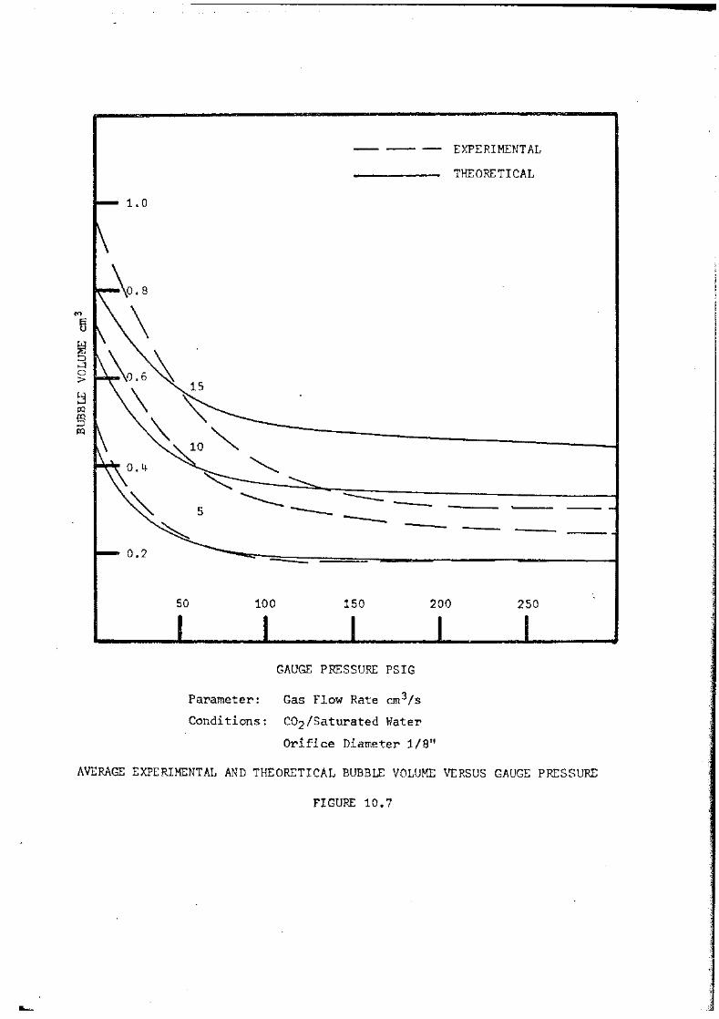
0.2
50
-- -- - EXPERIMENTAL
THEORETICAL
~ ---- -----------100 150 200
GAUGE PRESSURE PSIG
Parameter: Gas Flow Rate cm3/s
Conditions: co2/Saturated Water
Orifice Diameter 1/Su
250
AVERAGE EXPERIMENTAL AND THEORETICAL BUBBLE VOLUME VERSUS GAUGE PRESSURE
FIGURE 10.7

(\")
e r~ :E: !::) ~ 0 >
~ t:Q
§ 0.4 p~
-----5
50 100 150
GAUGE PRESSURE PSIG
Parameter: Gas Flow Rate cm3/s
Conditions: C02/Saturated Water
Orifice Diameter 3/16"
EXPERIMENTAL
THEORETICAL
-----
200 250
AVERAGE EXPERIMENTAL AND THEORETICAL BUBBLE VOLUME VERSUS GAUGE PRESSURE
FIGURE 10. S

"(8.
( 2 )_];he 1Sffect of f~~ystem Pressure for a Constant Flm·r Rate
Figure 10.6 and lO.B present the theoretical curves and the
smoothed experimental results for the terminal bubble volume against
system pressure for the three volumetric flow rates used in the initial
study. As in Chapter 6 the results shovr that after the initial marked
decrease in volume vri th pressure, the volu.rne rer.:tains nearly constant ,_
dropping only slighly with further increase in pressure.
The comparison between the predictions of the model and the
experimental results are particularly good for lo'-r gas flow rates
. through the larger orifice sizes, that is, for conditions 1-rhere the
single bubble model is most applicable. Whereas when the gas velocity
is high and consequently the liquid inertia large, as for the 11. 6 inch
orifice, the results do not compare as favo1u·ably.
In additlon McCann and Prince (22) point out that there may
be some variation in the shape of bubbles formed at small orifices
( .:$ 11 6 " ) when compared with larger ones. Small orifices follow the
Hayes et al (14) model for growth, where the surface of the bubble always
touches the perimeter of the orifice rather than the Dav:i.dson and Schuler
( 11) model where the bubble grows out along the orifice plate ( cf. Figure
1. 4). 'J'he results would appear to support the content·ion of McCann
and Prince (22) that bubble formation at small orifices needs to be
treated. separateJ.y from that a.t larger orifices.
(3) Tpe Effect of Liquid Depth
The height of the liquid seal above the orifice was varied
f'rom 2 to 6 inches. Although the model predicts a slight decrease in
the volume over this depth no variation in the experimental results could
be d.i s cerned. Other workers ( 14) ( 19) ( 39) conclude that at atmospheric
pressure the liquid seal has no effect on bubble size. However, this
is not conclusive since the predicted decrease in volume for a four inch

r
f")
5 ~ ::,:) ....:l 0 > ~ p:}
f8 .._)
t:P
o/
/ ~ 3Y
/
~ SYSTEM PRESSU~~SIG
/ /IJ
GAS FLOW RATE
0 5 cm3 /s
6 10 cm 3/s 0 15 cm 3/s
0
// 50
103
/
o/ 10~
/
0/ !So/
40.0 t ORIFICE REYNOLDS NU~ffiER ~::_,
'li'....toU
Parameter: System Pressure
Conditions: C02/Saturated Water
Orifice Diameter 1/16"
BLmBLE VOLUME VERSUS REYNOLD'S NUMBER
FIGURE 10,9
0/
/
n/
/
2oo» /
c{ LEIBSON ET AL (25)
/
g/
~
/
tY /
,
/o
-9fso 104

change in seal height is only about 2% '\vhich is of the order of
experimental accuracy. The apparatus was not suitable for testing
greater seal heights.
79.
(4) Comnarison with Hubble Volumes at AtmosJ2heric Pressure
It l1as been common practice to plot the results of bubbling
studies at atmospheric pressure in the form of average terminal volume
or diruneter against orifice Reynold's Number ( 25) ( 69). These studies
have found a straight line relationship.
There seems little justification for the use of Reynold's
Number in these correlations as neither the gas density nor viscosity
was varied substantially, the only variables being flow rate and orifice
diruneter.
The validity of a Reynold's Number correlation is tested for
the experimental result for the 1"1. 6 inch orifice on Figure 10.9. Lines
of constant gas density are drawn through the points to enable direct
comparison vTi th the results obtained by Lei bson et al (25). Under the
.same conditions (atmospheric pressure) the volume is a positive function
of' Reynold's Number which differs from the slightly decreasing function that
Leibson et al (25) found. The variation of gas density alters the
position of the constant density curve but not the slope. It is con
cluded that, when the gas density varies considerably, the volume cannot.
be related in a simple manner to the orifice Reynold's N~~ber. The
relationship between bubble volume and Reynold's Number found by Leibson
et al (25) was not confirmed.
1:_0 .l.J.. 3 Bubble Frequency
The experimental ancl predicted bubble frequencies are plotted
against flow rate on Figure 10.10, 10.11 and 10 .12. The experimental data at
atmospheric pressure agrees with that of other investigations (10)(19)(20).
.

(/) ........ (/l
~ a:l rQ ....... ~
)-t (.)
z f§ 0
~ J-'-1
...
0 0 PSIG
C;::J 50 PSIG
40
~
~~
30 00
!X] C()
20
~
0 0
c::J ~
lXI C:J
C(J
<> oo 0
0
0 <>
<>
00
GAS FLOW RATE cm3/s
Parameter: System Pressure PSIG
Conditions: C02/Saturated Water
Orifice· Diameter 1/16"
0 0
EXPERIMENTAL AND THEORETICAL BUBBLE FREQUENCY VERSUS GAS FLOW RATE
FIGURE 10.10

0
(;:::J
~
40
tn 30 ........ Cl.l
~ ~ ~ !::::) ~
t z ~ 0
~ tL..
0 PSIG
50 PSIG
150 PSIG
6
6
5
(j [j
<> 0
0
0
10 15 20
GAS FLOW RATE cm3/s
Parameter: System Pressure PSIG
Conditions: C02/Saturated Water
Orifice Diameter 1 I 8"
150
oo
25
EXPERIMENTAL AND THEORETICAL BUBBLE FREQUENCY VERSUS GAS
FLOW RATE
FIGURE 10.11
·o

---------------------------------------..~
40
30
0 0 PSIG
()(} 50 PSIG
~ 150 PSIG
5
o<>
10 15
150
0 0 0 0
20 25
------~-··~···-·~ __ _,_ ____ ..... ........., ____ ....., ____ -.lli _____ adil
GAS FLOW RATE crn3/s
Parameter: System Pressure PSIG
Conditions: C02 /Saturated vlater
Orifice Diameter 3 /16"
EXPERIMENTAL AND THEORETICAL BUBBLE FREQUENCY VERSUS GAS FLOW RATE
FIGURE 10.12

1.2
1.0
&IU-0.8
f'l')
t3
~ :::J H 0.6 0 :> w ....::l ti1 ~ ::J C.Q
0.1+
0.2
.......__
0 10
I
FREQUENCY BUBBLES/s
Parameter: System Pressure
Conditions: C02/Saturated Water
Orifice Diameter 1/8"
0
~
0 0 0
0 PSIG 50 PSIG
100 PSIG 150 PSIG 300 PSIG
/
50
CROSS PLOT OF EXPERIMENTAL BUBBLE VOLUHE AND FREQUENCY
FIGURE 10.13

80.
!J.lfle moclel predicts the general shape of the experimental
curves. For a fixed gas chamber volume, the increase in flOi·T rate
causes the frequency first to increase then to reach a nearly constant
value, the so-called maximwn frequency (18 )(70).
Discrepancy bet-v1een the model and experiment must result
because the theory only deals lvi th single bubbles and does not attempt
to model the interaction between bubbles vrhich occurs at high flow rates.
At high mass flow rates the gas imparts considerable momentum
to the liquid forcing the liquid in the centre of the column up-vrards.
Circulation is then set up dovm the side 1v-alls and across the orifice
plate. The cross flo-vr of liquid at the orifice will increase the fre-
quency above that of bubbles formed in a quiescent pool ( 10). This will
contribute to the discrepancy in the predicted results.
In a study of the turbulent bubbling region Calderbank (8)
observed a "constant frequency chain-bubbling" at about 20 bubbles/
second. Calderbank (8) reports that this value was independent of gas I
flow rate, orifice dimensions and physical properties of the gas and
liquid. Davidson and Amick (18) on the other hand correlate a limiting
frequency with volumetric floi-r rate and orifice radius.
Recently it has been shown (19)(20) that gas chamber volume
also affects the maximum frequency, but for any particular volume a
definite maximum still exists. The experimental results for maximum
frequen~y at atmospheric pressure exhibit both a dependence on flow
rate and orifice size. But Figures 10.10 to 10.12 also show· that the
maximum frequency is dramatically changed by increasing the gas density.
It is evident that gas density ought to be included in maximum frequency
correlations.
The influence of gas density is emphasised by Figure 10.13,
a cross plot of bubble volume against frequency. At atmospheric an
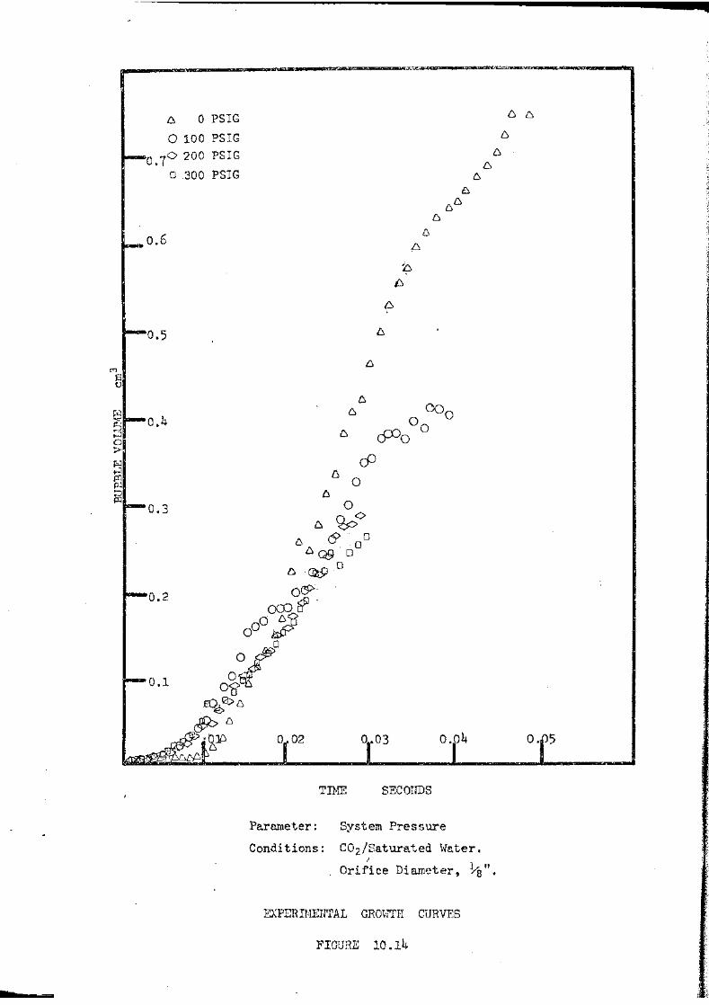
,,., s tJ
r:il s 0 ~
f':i1 ...:! f.i'1 P4
~
-
~ 0 PSIG
0 100 PSIG
0 ..,o 200 PSIG • I
o .300 PSIG
lit 0.6
0.5
0.4
0.3
6 '
0.04
TIME SECONDS
Parameter: System Pressure
Conditions: C02/Saturated vlater • .'
Orifice Diameter, Ya ".
EXPERD:IEUTAL GRm·ITH CURVES
FIGURE 10 .ll~

0.7
0.6
0.4
0.3
0.2
0.1
0.02 0.03 0.04 0.05
TIME SECONDS
Conditions: C02/Saturated Water
Orifice Diarneter., 1,.-8 u.
System Pressure, Atmospheric
EXPERINENTAL AND THEORETICAL GROWTH CUHVE
FIGURE 10.15

0.7
0.6
0.5
M
~ (')
el o.4 5 ~ 0 > ~1 .. .:t tQ f.'Q ~
P'-1 Ot3
0 .. 2
0.1
--·
0
0.02
0 0
0.03
wwzv:w::: mz nm• u~
0,04
TIJ-.1E SECONDS
0 05
Conditions: C02/Saturated Water
Orifice Diameter • Jys". System Pressure, 100 PSIG.
EXPERIMENTAL A~'D THEORETICAL GROWTH CURVE
l•'IGURE 10 .16

0 .. 6
0.5
1/'(')
f3 ()
t~ 0.4 s ~ 0 > f:t1 ....:1 &rl P:J
~ 0 .. 3
0 .. 2
CJOO o·
<>
TIME SECONDS
Conditions: ·co 2/Saturated Water.
Orifice Diameter 1;8n.
System Pressure, 200 PSIG.
EXPERIMENTAL .MTD TifEORETICAL GROWTH CURVE
FIGUHE 10.17
0.05

('f)
fl ()
~ :::;{ I-I 0 > r.-il ....:l t:4 P'~
~
--
0.7
o.6
.4
TIME SECOlifDS
Con.ditiong: C02/Saturated Water
Orifice Di~t.rnettn"', 1;-a". System Prc-ssu:re, 300 PDIG~
EXPF.RH~li:l'AL AND 'l1IEORETICAL GHOWTH CUHVE
FIGURE 10 .. l8

81.
increase in flo"t..r rate is achieved by first the frequency increasing,
the bubble volume increasing only slovly. At higher flo'r rates the
frequency remains constant but the bubble volume increases. At pressure
above 100 psig ,.rhere the gas momentum commences to make a signif'icP.nt
contribution to the grm.rth, an increase in flow rate results in r·. simul
taneous increase in both frequency and bubble volume.
10 .l~. 4 Bubble Gro1rth
rrhe volu..me of the forming bubble as a function of time is
plotted on Figure 10 .1ll to 10. J.8. The experimental points a.re from high
speed films taken at 1~000 frame~3/second in the manner described in
Appendix 2.
Figure 10.14 illustrates the differences in experimental
bubble growth for the range of system pressures. Several points are
noted:-
(1) An essentially similar growth curve occurs at all pressures.
(2) A higher rate of growth in the latter stages of formation
occurs at atmospheric pressure than at other pressures.
Figures 9.3 indicates that this is caused by the contri
bution to the upvard forces of the buoyancy plus gas
momentum decreasing v-ri th increasing pressure.
(3) As expected the increased gas momentum terminates the
g:r•ovrth a:t an earlier stage.
Figure J.O .15 to 10 .18 compare the experimental growth with
that predicted by the model. The agreement is good. The present model
more closely simulates the growth of the bubble than does the adapted
model in Chapter 6. The model, ho-vrever, still has the following deviations
from the experimental res~lts:-
(1) It underestimates the resistance to growth in the early
stage of formation.

Orifice
Diameter
PSIG
0
150
300
----
1..< " 16 ~" 8 316"
EXPERIMENTAL FLOW RATE, em 3 / s
5 10 15 5 10 15 5 10
PREDICTED FLO'v RATE, cm 3/s
5.1 10.2 15.3 5.1 10 .. 3 15.3 5.5 10.6
5.1
4.6
7.8 9.7 5.1 8.6 11.6 5.6 9.2
6.8 8.3' 4.9 8.3 11.1 5.4 8.3
COMPARISON OF AVERAGE EXPERTI1EUTAL AND
THEORET I CAL :B.,LO\v RATES
FIGURE 10.19
15
15.2
12.3
12.1
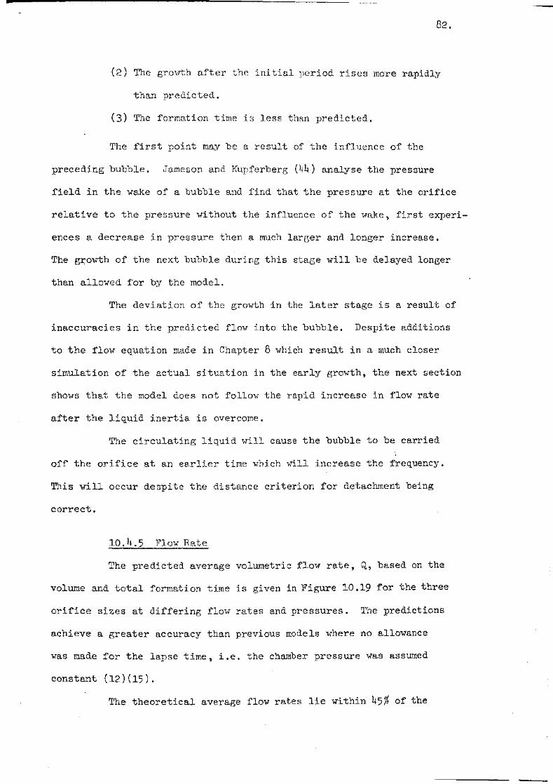
82.
(2) The grovrth after the initial period rises more rapidly
than predicted.
(3) The formation time lr:> less than predicted.
The t"irst point may be a result of the influence of the
preceding bubble. James on and Kupferberg (l.~4) analyse the pressure
field in the wake of a bubble and find. that the pressure at the orifice
relative to the pressure without the influence of the vrake, first experi
ences a decrease in pressure then a much lare;er and longer increase.
The gx:-owth of the next bubble during this stage will be delayed longer
than allowed for by the model.
The deviation of the growth in the later stage is a result of
inaccuracies in the predicted flow into the bubble. Despite additions
to the flow equation made in Chapter 8 which result in a much closer
simulation of the actual situation in the early growth, the next section
shows that the model does not follovr the rapid increase in flow rate
after the li~uid inertia is overcome.
The circulating liquid w:i.ll cause the bubble to be carried
off the orifice at an earlier time vrhich 1vill increase the fre~uency.
This will occur despite the distance criterion for detachment being
correct.
10 .lL 5 Flow Rate
The predicted average volumetric flow rate, Q, based on the
volume and total formation time is given in Figure· ~0 .19 for the three
orifice sizes at differing flow rates and pressures. The predictions
achieve a greater accuracy than previous models where no allowance
was made for the lapse time, i.e. the chamber pressure was assumed
constant (12)(15).
The theoretical average flow rates lie within 45% of the

/"' 25 I \ --- -- EXPEHIMEN•rAL
I \ THEORE'I'ICAL
I \ (J} 20 .........
\ M
J-1
I (J
rx:l 8
~
I \ ~ 15 0 1-1 j:J..
UJ
I \ .c:t: 0
\ 10 I \
5 I \ \ I
I TD-1E SECONDS
Conditions: C02/Saturated Water.
Orifice Diameter, 113". System Pressure, Atmospheric.
EXPERIMENTAL AND THEORETICAL INSTANTANEOUS FLO\<! RATE
FIGURE 10.20
-=-
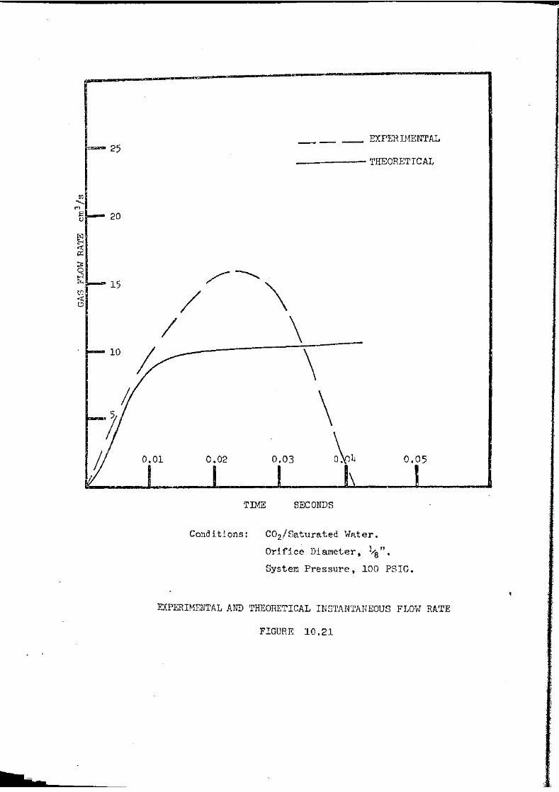
--- EX PER IHENTAIJ ~ 25
----- THEORETICAL
1) /~·
/ \ I \
10 i \
111.-.a ....... ___ _
0.01
\ 0.02 0.03 0.05
TIME SECONDS
Conditions: C02/Saturated Water.
Orifice Diameter, Y8 11
•
System Pressure, 100 PSIG.
EXPERIHENTAL AND THEORETICAL INSTANrl,ANEOUS FLOW RA.TE
FIGURE 10.21
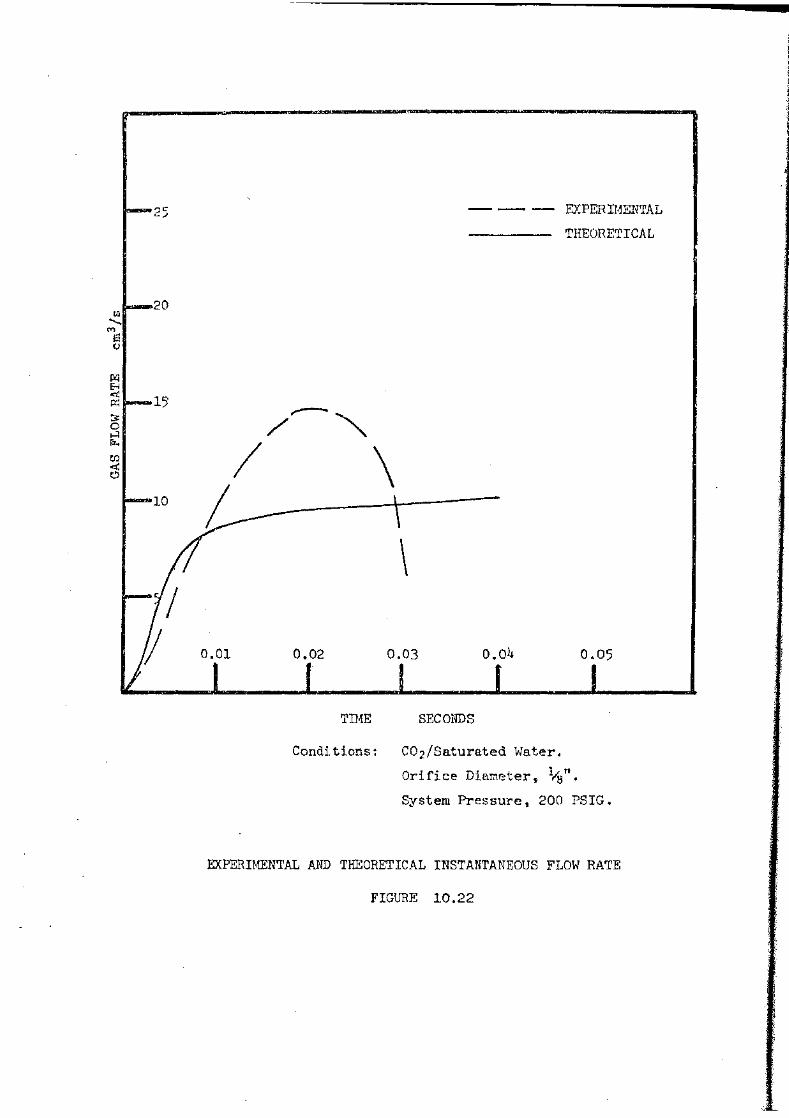
25
20 til
......... M s
(J
M E-1 <i!
1) ex: ~ 0 ...:! ~<1
00 oct, e>
10
0.02
\
0.03
- - - EXPERIMENTAL
THEORETICAL
o.o4 0 .. 05
TIME SECONDS
Conditions! C02/Saturated \rlater.
Orifice Diameter~ 1/s". System Pressure, 200 PSIG.
EXPERIMENTAL AND THEORETICAL INSTANTANEOUS FLOW RATE
FIGURE 10.22

25
10
0.01 0.02
\ \ \
- - -- EXPERIMEnTAL
THEOHETICAL
o.ol~ o.o5
~~~--~~rm-~~-..1.---L,~ TIME SECONDS
Conditions: C02/Saturated Water.
Orifice Diamete-r, 113 u.
System Pressure, 300 PBIG.
EXPERHfENTAL AND THEORE'fiCAL INSTANTANEOUS F'LOW RATE
FIGURE 10.23

83.
experimental value over the range 1 to 15 cm3/s and 0 to 300 psig, with
an average deviation of only 15%. At pressures near atmospheric the model
overestimates the flow rate but at higher pressures the average flow rate falls
below the experimental value. The deviation is caused by inaccurate esti-·
mation of the formation period. In Figures 10.1'7 and 10.18 the model
estimates a significantly larger formation time than found experimentally,
through failure to allow for bubble interference and liquid circulation.
A more exacting test is prediction of the instantaneous flow
rate. The experimental instantaneous flow rates from a least mean squares
:fit of the gro1vth curves are shown against the model instantaneous flow
rates on Figures 10.20 to 10.23. The theoretical :flow equation, -with the
inertial terms, models the floiv into the forming bubble reasonably during
the initial period. After overcoming the inertia of the liquid and the
pressure in the ;,.rake of the preceding bubble has abated (43) ( 41~) the gas
enters the bubble i.n a sudden rush, the flow rate then declines rapidly
before detachment.
The model appears limited in this period since it relies on
an artificial detachment criterion. To solve the analysis which would
be required to estimate the decreasing flow as the neck stretches, and
finally ruptures~ greatly increase the complexity of the solution. The
model could be 1.mproved more profitably in other areas.
10.4~~~bling Regimes
The bubbling regimes are classed according to McCann's (22)
description. The classification is essentially visual and represents
a gradual change from the predominance of one type of bubbling interaction
to the predominance o:f another, depending on flow rate and system pressure.
Bubbling with delayed release is distinguished from normal bubbling by
different pressure fluctuations in the gas chamber. A full description
of the various regimes is given in Chapter 1.

tr.l ........
ffl
s ()
~ ~ :.;: 0 ....:l ~
(/)
< (!)
·~ 30
DOUBLE BUBBLD'-!G
1:"" ./ /
SINGLE ·~ BUBBLING/ BUBBLING ~. TI·-II
DELAYED RELE~
\ . . (
/ / \
DOUBLE BUBBLING
WITH DELAY£ D RELEASE
\
200
\
HUI:fiPLE BUBBLIN(~
250 • 50 100 ~0
.J - J _l ~~~--...__-~
30 1/8" DIAME~ORIFICE
\ MULTIPLE BUBBLING
\ 20 \
DOUBLE
\ BUBBLING
\ \ ~ \
SINGLE"""
""" BUBBLING
~ ""' so ~ 150 200 250
" ----GAUGE PRESSURE PSIG
PHASE DIAGR~MS FOR THE CARBON-DIOXIDE-SATURATED WATER SYSTEM
F'I GUFl~ 1 0 • 211·

10 3dyn/cm2 -
zero
-10 3 dyn/cm2 --
PRESSURE VARIATION IN GAS CHAMBER CAUSED BY SINGLE BUBBLE FORHATION
(D0 =l/8", G.=l0cm 3 /s, Atmospheric Pressure.)
FIGURE 10.25

'11-le different regimes ob~::;erved are plotted against system
pressure and gas flow rate for the l,....B and 3/16 inch orifice on Figure
lo 24 It . h . d th t th 1' th. If 1 ff d. • . .· l s emp as1s e · ·- a · e 1nes on ls p 1ase lagram represent
a gradual transition from one region to another based on a subjective
assessment of the photographic record. The photographs, Figure 10.1
and 10.2 show the three main rer,imes for each orifice.
Each regime haB a eharacteristic cycle of gas chamber pressure,
· thus in order to properly describe these typ::~s of bubl)ling, the pressure
variations must be analysed. P~ short description of' each cycle is given
below to supplement the description of each regime given in Chapter 1.
Th1.s is folloved by comparison of the experimentally determined pressure
cycles with those predicted by the model.
Figure 10.25 shows the pressure variation in the gas chamber
caused by a single bub1Jle. Growth of the bubble connnences when the
pressure in the chamber rea.ches a value sufficient to overcome the
surface tension of the liquid meniscus across the orifice. Initially
the. flow into the chamber is greater than the outflow because the
inertia of the 1iquid surrounding the new bubble is large, hence the
pressure rises.. 'l1he chamber pressure reaches a maximum when the outflow
equals the inflow. As the velocity through the orifice increases further
the rate of bubble growth progressively outstrips the inflow into the
chamber and the pressure drops. After detachment the liquid meniscus
forms across the orifice and the pressure in the chamber increases as
before.
Figure 10.26 sho·ws the oscilloscope trace of the pressure
variation in the gas chamber superimposed onto simultaneous photographs
of double bubbling~ The pressure variation is sketched separately on

DOUBLE BUBBLING \VITH OSCILLOSCOPE TRACE OF GAS CHAMBER PRESSURE
FIGURE 10.26

Conditions: C02/Saturated Pressure
Gas Flow Rate 10 cm3/s
System Pressure 100 PSIG
Orifice Di&-neter 1 /8"
GAS CHAHBER PRESSURE FLUCTUATIONS FOR DOUBLE
BUBBLE FORMATION
FIGURE 10.27
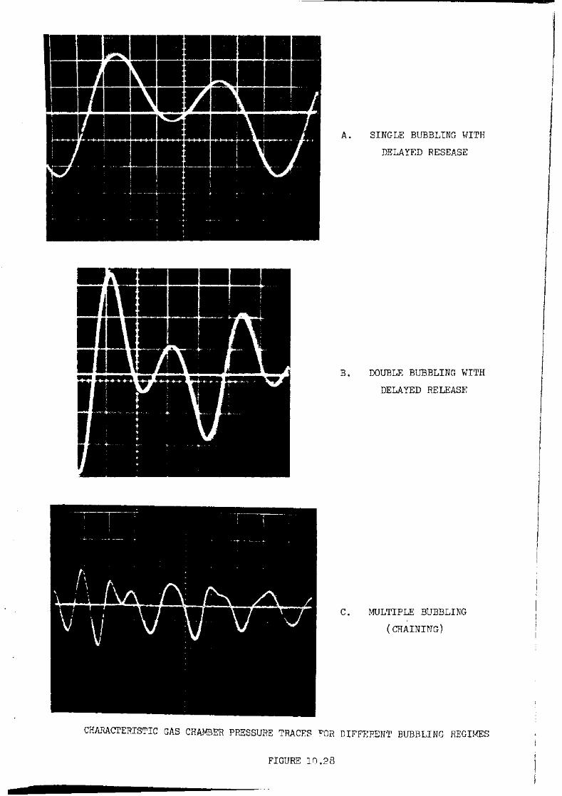
A. SINGLE BUBBLING WITH
DELAYED RESEASE
B. DOUBLE BUBBLING WITH
DELAYED RELEASE
C. MULTIPLE BUBBLING
(CHAINING)
CHk~CTERISTIC GAS CHAMBER PP~SSURE TRACES FOR DIFFERENT BUBBLING REGIMES
FIGURE 10.28

Figure J.O. 27. Although the photographs show· the second bubble is
elongated, indicatj_ng tlle effect of' the 1-rake of the first lntbble !I the
pressure fluctuation for each bu1)bJ.e in the gas chamber is not altered
from that produced by tvTO single bubbles.
Delayed release bubbling arises in certain conditions where
the pressure f'alls quickly, and the flow through the orifj.ce ceases, before
the bubble is fully formed. Instead of detachment taking place at this
point the bubble remains attached to the orifice and continues to rise
under buoyancy, adjusting its position on the orifice at constant volume.
A:fter the flow into the bubble has ceased or greatly diminished the pressure
builds up to a value sufficient to start the growth again and a second
maximum in pressure wilJ. occur as shown in Figure 10.28(a).
In the case of double bubbling with delayed release,. Figure
10.28 (b), the first bubble sho~rrs the pressure fluctuation characteristic
of delayed release but the second bubble exhibits the characteristic of
normal single ·bubbles. The reason for this, though not clearly understood~
:i.s thought to be a result of the influence o:r the wake of the first bubble
(19).
TJ:1e traces for double bubbling, or double bubbling with delayed
release, gradually merge into the mu.l tiple bubbling region where the
traces are irregular. For example, Figure 10628(c) shows irregular
pressure va:ciation in the gas chamber for bubbling at 300 psig through
the 3/1 6 inch orifice.
(2) Comnarison with Predictions of the Model --~·
':£!he model for the variation of gas chamber pressure proposed. by
Kup:ferberg a.nd. Jameson ( 20) and a similar one by McCann ( 19) have shown
good agreement with experiment for large capacity gas chambers. Both
,.,orks report the pressure fluctuations for a gas chamber volume of 2250 cm3
and a ~ inch orifice. In this study a gas chamber volume of 375 cm3 and

A.. Att'lospheric Pressure
Single Bubbling ..
B. 100 PSIG Single
Bubbling with
Delayed He lease
c. 200 PSIG Double
Bubbling with
Delayed Releas~
D. 300 PSIG
Multiple
Bubbling
Conditions: C02/Water
do ::. 3/16"
Q = 10 cm 3/s -5
DETACHMENT
/\ J \
\ 0.04
SECONDS
\ \ DETACHMENT
CO!l?ARISO:l OF GAS CHAMBER PRESSUP,E FLUC'l'UATIONS
FIGURE 10.29

86.
orifice diameters less than 316 inch a.re conditions -vrhich vrill severely
test the model since the capacity of the chrunber is small and the rate
of change of pressure is large.
The predicted pressure fluctuations for the 316 inch orifice
were tested at atmospheric pressure in Section 9. 8, Figure 9. 3 For these
conditions the model gives reasonable ae;reement with experiment for both
magnitude and period of the fluctuation.
Figure 10.29 presents the experimental and theoretical curves
for a f'low rate of 10 em 3 Is for the same orif'ic e over the range 0 to 300
psig. The experimental results confirm that stable, reproducible pressure
fluctuations are established in the gas chamber vhen single or double
bubbling occurs. The results illustrate the change from single bubbling
to multiple bubbling.
No theoretical allo-vrance has been made for interaction between
bubbles so it can be expected that the single bubble model will progress
ively differ from the experimental results as the experimental bubbling
regime changes from single bubbling to double bubbling and then to multiple
bubbling. This is confirmed by results w·hich show that the model fits
the experimental data more closely at low· pressures.
At pressures above atmospheric the single bubble model exhibits
a cyclic pressure characteristic of delayed release. The amplitude of the
variation at 100 psig system pressure is less than found experimentally.
McCann (19) also finds that the single bubble model he develops does not
match the delayed release fluctuations, he suggests a modified model
in which the bubble remains at constant volume while the chamber pressm·e
recovers. It is concluded ( 19), however, that the model is still inadequate
:for describing delayed release bubbling. No extension of this is under
taken in this work.
At 200 psig, where double bubbling with deJ.ayed release occurs,
I

the model still shows some agreement 1d th the e.xpe:r:i.mental trace for
the f':i.rst bubble but no account is taken of the second bubble. For
multiple bubbling the predicted fluctuation fails to match the experi-
men·t.al trace.
It is evident that the decrease in period of oscillation is much
greater for the experimental results than predj cted as the pressure
increases. This arises from increase liquid circulation which causes the
:frequency to rise above that occurring solely through increased gas
density.
Attempts to model the growth of the second bubble of a double
bubble or the delayed release bubble (19) have been only partially success-
:ful, as they soon meet with inordinate mathematical complexity. Failure
o:f the model to fit the experimental pressure plots accurately, in bubbling
regimes where the mod.el does not strictly apply, is not a severe limitation
on its applico..bili ty, since these variations are transient, and in both
directions with respect to the second differential of volume V. Hence,
by the inclusion of' the expression of this variation in equation 9.3, it will
. affect the flow rate, V, and to a less extent the volume V. However,
the moclel still leads to reasonable terminal volume and growth :predictions.
10.5 Conclusions
The study has demonstrated the behaviour of carbon-dioxide
bubbling f'rom a single submerged orifice over a ,.ride range of system
variables. From consideration of an idealised :picture of a single bubble
:forming~ which included the inertia of the liquid surrounding the forming
bubble and the rate of change of gas momentum, quantitative predictions
o~ volmne, frequency, grovnh and flow rate and the pressure variation in
the gas chamber have been obtained for system pressures up to 300 :psig
and f'low rates f'rom 1 to 30 cm3 /s.

In particular, the mode :.1kes good predictions of the :volume
and gro1·rth for this pressure ranee for flow rates below 15 cm3 /s. For
the remainder, the theory describes the trends of the experimental results
but increasing discrepancy between the model and experiment occurs
because the theory only deals vri th single bubbles and assumez that no
interaction between bubbles takes place at high mass flow rates. For
these conditions liquid circulation also becomes a major consideration.

C'f')
~ ()
~ ;E ::::> ...:I c ::> J.~,:
........ r~ p:::j ::.J 1-Q
...:l < E-t z ~ H ~ w
~
1.4
1.2
1.0
0.8
0.6
0.4
0.2
0
6
0
0 0.2
Orifice
3/16"
1/8"
1/16 tf
Diameter
60
6 0
0
0
~
6 0 0
0 ~
~
0
6 0
0 00
6 ol:l.
0
6 0
0.4 0.6 0.8 1.0
PREDICTED BUBBLE VOLUMP. cm3
EXPERIHENTAL BUBBLE VOLUHE VERSUS BUBBI..E VOLUME PREDICTED BY
MODEL, CHAPTER 9, FOR CARBON-DIOXIDE- HATER SYS'I'I:M

CHAFCEH 11 ---~,. .... ,~-
DISCUf)SION OF 'IJJ~ 11m0RETICAL ANALYSIS
This chapter stunmarises the success and limitations of t.he
theoretical analysis, in particular the influence of liquid circulation
on the theoretical predictions is discussed.
11. 2 The Model
The model developed in this 1-rork has shown a significant im-
provement over similar models in its ability to predict the volume and
:flow rate of singly formed gas bubbles. The improvement results from
incorporating terms to describe the liquid inertia caused by vertical
and radial movement o:f the forming bubble.
The a.ddi tion of a term for the gas momentum has enabled the
model to 1)e extended to cover situations, such as high pressures,. where
the gas density has significant influence on the rate of growth.
Chapters 7, 8 and 9 discu.ss, in depth, the development of the
model. In those chapters the equation of motion and the energy equation
of the growing bubble are presented and their solution described.
The sensitivity of the model to changes in the variables is
given in section 9. 8, where the predicted growth curves and the parameters
ef'fecting growth are also discussed.
In Chapter 10 satisfactory agreement between volume and growth
rate was obtained. rrhe success of the theoretical analysis in matching
the experimental pressure fluctuations in gas chamber under severe physical
conditions vras also discussed.
Figure 11.1 plots the predicted volume against experimental
volume for the range of pressures and flow rates covered in this study.

90.
As expected the model sho'!.·rs a vrider variation at large volumes (that
is, high flm.; rates) where the "single" bubble model does not strictly
apply. The overall agreement is good with an average deviation of 20%
over the whole range. The maximum deviation is 40% while the descrepancy
at low flow rates is much smaller.
As pointed out earlier, in order to proceed with an analytical
analysis it vras necessary to make certain assumptions - some of which
are not strictly valid.. As the ability to model simple si tuat:i.ons improves
so it will become possible to attempt to eliminate some of these simpli
fications. 'I'he present model has the following major limitations:-
(1) TI1e bubble is assumed at all times to be spherical.
(2) Liquid circulation is neglected.
(3) Viscous effects are ignored.
( 1.~) The motion o:f the bubble is not effected by the presence
o:f any other bubble.
( 5) Gas circulation within the bubble is not considered ( 5) •
(6) The effect of the orifice plate is negligible (20).
It is proposed in this chapter to discuss only the first four
limitations, these being considered the more important to the present
study. The other limitations are discussed in the references given.
11.3 Liquid Circulation
The e:ff'ect of liquid circulation is difficult to account for
theoretically. It has been the practice to design the experimental appa
ratus so that the bubbles can form in as stagnant a region as possible.
This has been partially achie,red by the addition of' a perspex ring ( 11)
or" as in this work~ the use of a raised orifice plate.
Liquid circulation is of particular importance in high pressure
reactors where the rapid formation rate causes an increase in the rate
of liquid circulation by virtue of the increased momentum transfer to the

91.
liquid. !J.lds section sets out several approaches to the problem and
points out the difficulties of incorporating them in the model.
The manner in vrhich the circulating liq_uid will affect the
growing bubble is complex, involving both horizontal and vertical com-
ponents of momentum over the gas-liquid interface.
The overall effect is to S"\veep the bubbles off t.he orifice,
giving rise to a higher frequency and smaller volume than :l..f they were
formed in a stagnant pool, (10) (23).
Davidson (71) suggests that a very simple approach may be used
to demonstrate the effect of an upward liquid velocity at the orif'ice.
Consider a bubble forming at a point source in a liquid stream moving
upward at a velocity ui. At time t since the bubble began to form its
centre.has moved a distance, s, that is,
s = u t .Q,
11.1
'Ibis is provided ui is sufficiently large for the bubble acceleration
due to buoyancy to be negligible. Now assuming constant flow rate into
a spherical bubble, the radius a at time t is,
= Qt 11.2
If detachment occurs say,at a= s,then by eliminating t from 11.1 and
1~. 2 the bubble radius is given by~
11.3
Thus, from this obviously over simplified argument,it can be show~ that
an increased liquid velocity would decrease the bubble volume and con-
sequently increase the frequency.
The limitations of this approach are that the circulation is
unlikely to be so great that the motion can be considered as entirely
due to the upward liq_uid velocity and the simplified model neglects the
horizontal liquid :flow. Measuring the liquid velocity vrould also be a

I·
h
c
BUBBLE CHAtffiER WITH DRAUGHT TUBE ( REFF:RENC:L 72)
FIGURE 11.2
·---------------

92.
problem. Freedmar1 and Davidson (72) have developed two alternatiye
approaches, the "gulf-steam" and the "draught-tube" which lead to the
prediction of the upvrard lic1uid velocity induced by a. pnrticular gas
flow rate.
r:ehe 'gulf-stream" model is based on a simple vortex pattern and
the manipuJ.ation of a stream function to obtain the velocit.y components
at any position. The "draught-tube", which will be discussed in greater
detail, is based on a forced circulation pattern up a. central thbe and
down the annulus (Figure 11.2). Although it is not clear how fo::r thee:(~
regimes are quant:i.tatively relevant to the flow pattern vrithout the
d.raught-tu.be, there is a clear qualitative si.mila.ri t:r. However !I neither
approach attempts to relate the effect of the liquid f'lo"\v on the forming
bubble.
Referring to Figure 11.2 it is found experimentally (72) that
the pressure is uniform aeross the top of the liquid column, that is
P1 == P3. At the orifice plate it follows from a pressure balance in the
liquid that,
11.4
where en a.nd E A are the bubble volume fractions in the tube, area An,
and the annulus, area A A.
~lflus,
I 110r continuity,
and by manipulation,
2 2 2gh£n(A - AD)
Vn = ----------------------An2 ( 1 - e: D)
2 + (A - An) 2
11.5
11.6
11.7
This study involves a single orifice, with bubble behaviour inclfding
chaining, under 2 inches o:f water • Consider a chaining situation

Table 11.1
Effect of Initial Upw-ard I:,iquid_Veloc:!:J~}[_0l
Pl"'edictions of the Model.
Conditions:
Atmos-pheric Pressure
Initial Up\vard Velocity (cm/s)
0
10
100
300 PSIG
0
10
100
-----------------
C02 /Saturated Water
Orifice Diameter 1/8 "
Gas Flow Rate 10 cm3/s
Volume (cm3 )
0.66
0.64
0.58
0.32
0.28
Frequency Bubble/s
15.5
16.0
17.5
32.7
33.0
33.9

93.
in which the average bubble diameter is 1 em and assume that no gas
bubbles are carried back do-~·m the annulus,. e:A = 0 ~ ancl that the area
for upward liquid flow equals that for dovmward flow, i.e. for this
study An = AA ~ ho cm2 • Then,
e: = D
=
Vol. of bubble X no. in h
AA X h
. • 0.013
By substitution into equation 11.7,
Vn ~ 20 em/sec ..
By manipulation of the :flmr areas so that~ say the area of the draught-
tube has a diameter of only twice that of the bubble, then it is possible
to obtain,
Vn = 100 em/sec.
That is, of the order of magnitude of the gas velocity.
The flo-vr area is not easily measured and the effect of upward
liquid motion ha.s been tested only to a very limited extent. This has 1Jeen
done by initiating bubble formation with an upward velocity previously
asslL'rlled zero. 'I'able 11.1 indicates the effect of impo_sing an initial
Uin·rard velocity of bet1-reen 10 and 100 em/ sec on the model for a gas flow
rate of 10 cm 3/s. The results follow the trends envisaged but not to
the degree required.
The motion of the liquid, of course, effects the growth throughout
formation not just at initiation. Horizontal motion has also been ignored.
The use of stream functions (72) may be able to deliniate the
:flow areas and provide the horizontal velocity components. The problem
still remains of relating the liquid motion to the bubble growth. This
problem seems to be one of the major tasks facing the advancement of

94.
theoretical models, particularly in high pressure systems. It wo~ld appear
that sui table experimental apparatus could be made to measure the strength
of' a deliberately induced bulk flov" Further d~velopment, however, is
beyond the scope of this investigationQ
11.l~ ...!:-Sphericity
It has been assumed that the bubble grows a.s a. sphere or portion
of a sphere. From the photographic evidence it can be seen that this
assumption appears reasonable near atmospheric pressure but at higher
pressures particularly for the smallest orifice a spherical shape does
not portray the physical situation.
The dilermna faced in this situation is that if the assumption
of' sphericity is retained, "exact" solutions may be obtained from the
model where as if the non-spherical nature of the bubbles is to be taken
into account, then, to avoid inordinate mathematical complexity, the use
of' empirical relationships will result.
The ability of the model to cope with non-spherical situations
appears to justify the former approach. Some work of Collins U18) for
extremely hie;h gas velocities where the bubbles v..rere anything but spherical
showed that the assumption of sphericity gave reasonable results.
The enlargement of the surface area caused by deviation from a
sphere is generally over-estimated. If the deviation is expressed as
the sphericity (surface area of a sphere having the same volume/actual
surface area) then, even in the case o~ severe departures, for the most
part, the deviations are not essentially smaller than 1. For instance
:for a cube the sphericity is 0. 7.
It seems reasonable to conclude that shape is not the most
important consideration during the growth, the ratio of the various
:forces acting being more important.
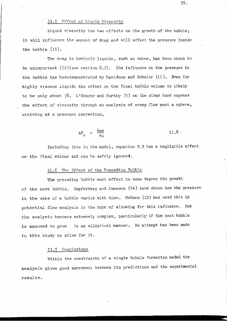
95.
11.5 Effect of Liauid ViscositY ..... _ .. _"-- -------~·--~
Liquid viscosity has two effects on the grm-1th o:f the buhble;
it 1vill influence the amount of drag and will effect the pressure inside
the ·uubble (1.1).
The drag in invi scid liquids, such as \-Tater, has been sho¥rn to
be unimportant ( 12) (see section 8. 3). The influence on the pressure in
the bubble has beendemonstrated by Davidson and Schuler (11). Even for
highly viscous liquids the effect on the final bubble volume is likely
to be only about 3~{,. L'Ecuyer and Murthy (5) on the other hand express
the effect of viscosity through an analysis of creep flow past a sphere,
arriving at a pressure correction,
11.8 .
Including this in the model, equation 9.3 has a negligible effect
on the final volume and can be safely ignored.
11.6 The Effect of the Preceding Bubble
The preceding bubble must effect to some degree the growth
of the next bubble. Kupferberg and Jameson (44) have shown how the pressure
in the wake of a bubble varies with time u McCann (19} has used this in
potential flow analysis in the hope of allowing for this influence. But
the analysis becomes extremely complex, particularly if the next bubble
is assumed to grow in an elliptical manner_ No attempt has been made
in this ·study to allow for it.
11.7 Conclusions
Within the constraints of a single bubble formation model the
analysis gives good agreement between its predictions and the experimental
results.

96.
The model can be used to describe the effect of increased
system pressure on the formation process. rl,he most serious obljection
is that the model does not allow for the e:f:fect of liquid circulation
which is of considerable importance in high pressure reactors. Several
approaches have been outlined but need to be persued further.

97.
CHAP1'EH 12 ------.. --GE:ilE.TIAL CONCLUSIONS ----~···------- ... - .. .._ .. .; __ _
This study has i. trated the differences in ga.s bubble
format.ion from a single suL .. · rged orifice as the system pressure in-
crea.ses. '.rhe specific conclusions at the end of' each chapter may be
sunnnar i sed.
( 1) It has been shown that for the same volumetric flovr :r.ate
increased system pressure causes smaller but more frequent
bubbles to be formed. Bubbling at high mass flow rates is
characterised by a large degree of interaction and coal-
escence near the orifice.
(2) rrhe theoretical analysis has shovm that a two stage model
adapted for the system conditions has fundamental inadeg_uacies
in the formulation of its equations to describe the growth
of the bubble. It was found that in obtaining comparative
simplicity of the mathematical solution of the equations~
realism was severely affected.
(3) A continuous model for a single bubble was developed to
overcome this defficiency. The grmvth of the bubble was
described by an equation of motion and an eg_uation of energy
of the expanding interface. This model included terms for
the inertia of the lig~id surrounding the bubble and the rate
of change of gas momentum issuing through the orifice.
( l~) Incremental solution of the equations has been used to cal-
culate bubble size, frequency, growth rate and instantaneous
flow rate for a range of average gas flow rate and system
pressures.

98.
( 5) Hi thin the constraints of the singJ.e bubble mod.el the
ana1ysis sho1vs good agreement for voltune and flm-r rate,
and predicts the correct trends for the other parameters.
12. 2 Rcope for Further Work
In essence this study is an initial survey of an aspect of gas/
liquid behaviour '\·lhich has received little attention to date. Thus the
:follo-vring aspects are but a few important areas for further investigation
from many directions which this field might take.
( 1) A significant area of experimental study still to be investi
gatE-)d is the behaviour of gas bubbles near the critical
pressure of the gas, where the liquiCl./ gas density ratio
tends to l.
(2) 1neoretically there appears two main limitations on the
applicability of the model,
(i) Liquid Circulation
(ii) Bubble Interaction
Both problems are very complex. It would seem that the
influence of liquid circulation on bubble formation would
be the easiest to investigate and allow for theoretically.
(3) It would be logical to extend the theoretical work to mass
transfer during formation at high pressures.

APPENDIX 1. -----·------The I~!:S~r.crties .S?LC2.f.trbon Di<2_;<ide -
\Vc:l,ter S;tEtem Under Pressure.
Al.l Densit_x_
Li9.uicl Densit~:
The densities of water saturated with carbon-dioxide are
99.
presented by Parkinson and De Nevers (73). Their graphical presenta.tion
of results for density of solution as a function of' system p:r.essu:re may
be interpolated ancl expressed in the form of an equation for ease of
comput.Rtion.
0 For 20 C and 0 < P < 500,
p -0.0063(P + 14.7) + 448.965
450
"rhere p is in gm/cm 3 and P is the gauge pressure pressure in psig.
Ga~ Densi~:
0 Gas density for C0 2 at 20 C has been taken from the International
C:r.i tical Tables ('74) and may be expressed as,
p' = 0.00183 + 0.0001224 p
For 0 < P < 500,
where p 'is in gm/cm3 and P the gauge pressure in ps:i.g.
~ Viscosity
Liguid Viscosity:
'l'he viscosity of liquids below the normal bo:i.ling point is
not particularly affected by moderate pressures. But under very high
pressures large increases have been noted. Water is an anamoly (75)
increasing only t."t.ro fold from 1 to 10,000 atmospheres. Variation of the
viscosity of water in this study can therefore be safely ignored.

100.
Gas Viscosity:
The gas viscosity calculated f'rom the equations of state
given by Reid and Sherwood (75) varies from 0.0147 cp at atmospheric
pressure to 0.0162 cp at 300 psig.
Al. 3 Surface ':Pension
The value of surface tension for water at 20°C was taken as
72 dyne/em. Surf·ace tension decreases as the pressure is increased
owing to the increased solubility of the gas. From the limited data
available (76) it would appear to decrease linearly to a value of 81%
that at atmospheric pressure at a pressure of 300 psig.
This variation is expressed as,
a= 72 (1 - 0 · 194~ P) 29
Ap1)licable over the range 0 < P < 300, where a is in dyne/em and P is in
psig.

y
etc.
BUBBLE OUTLINE FOR VOLUME CALCULATIONS
FIGURE A2 .1
•
h
Increment h was chosen to give a value of n p;:reatt:r than 30.

101.
APPENDIX 2.
A2 .1 Method of Data Reduction
The experimental data was recorded on motion picture films
which are availab]e from the Department of Chemical Engineering of the
University of Melbourne.
The volume of the bubble at any instant during :formation was
determined from the frames of these high speed motion pictures as follows:-
( 1) The film vras projected onto a ground glass plate in a
commercial motion picture analyser. The co-ordinates of
the bubble image were aligned by cross hairs and the x-y
co-ordinate data automatically recorded onto punched paper
tape.
(2) The outline of the bubble was recorded by dividing the
y-plane into a series of equal increments of width h,
and determining the x-ordinate, as shown on Figure A2.1
(3) The data was then analysed on the computer as follows:-
Consider the chord lengths lo, l1, l2•••• ln, equally
spaced by the distance h, where lo = xo1 - Xo2,
l1 = Xll - x12, etc., as shown on Figure A2.1.
Then the volume of the bubble is approximately given by
Simpson's rule.
V = ~ (Ao +An+ 4(AI + A3 +As+ ..• An_ 1 )
2 (A2 + A4 + A6 + · · .An-2 ))
where A - !. 1 2 i - 4 i
+
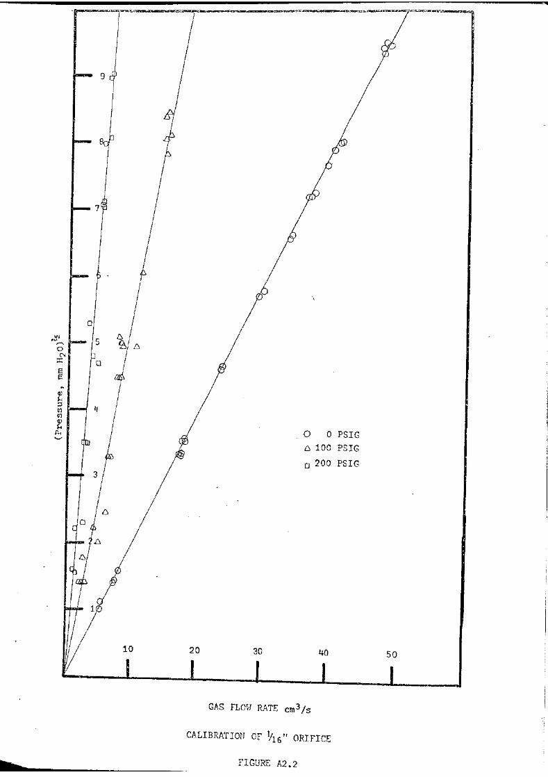
9
8
7
0
-
10 20 30
0 0 PSIG 6 100 PSIG
o 200 PSIG
40
GAS FLOH RATE cm3 /s
CALIBRATION OF !fiG" ORIFICE
FIGURE A2 .. 2
50

102.
The results u:::d.ng Simpson's rule were also checked ~gainst
two other similar methods, the trapezoidal rule, and
Wecldle 's ~ rule (56). Deviation ~etvreen these methods
was less than 2%.
( ~.) The true volume was computed by mul tip1ying the volume by
a scale factor obtained from the film.
A2. 2 Calculation of Instantaneous Flow Rate
The bubble volume was measured for a series o~ frames as
described above. The time 1)etween frames was determined from the timing
1 light -vrhich impinged onto the side of the film every 'i o oth second.
A growth curve was constructed from these two measurements (e.g. Figure
10.14).
The series of experimental points (Vi, t) was then fitted by
a least mean squares method ( 81) of the form,
It was found that a fit to the third power gave agreement to. within 4%
of' the experimental points.
The expression for volume was differentiated and the flow rate
at any time within the growth period determined.
A2.3 Evaluation of Orifice Coefficient
The orifice coefficient was measured from the relationship
between flowrate and pressure drop for gas flow through the dry orifice.
Figure A2.2 shows the experimental results ~or the 116 inch
diameter orifice. The slope of the plots at different pressures is given,
with an accuracy given below, by the expression ( P ~ )~ •
From the graph the orifice coefficient was determined. These
are summarised as,

103.
Orifice Diameter Orifice Coefficient ( .· ;b)-~---1nch (em~)
116 0.022 ± 0.0005
1~ 0.024 ± 0.0005
316 0.025 ± 0.0005
A2. 4 Precision of Determination of the Heasured Variables
Gas Flow Rate, Q •••••••••• ±1%
System Pressure, P • • • • • • • • • ±1%
The percentages represent instrument accuracy of the equipment
used to determine the variables, i.e. wet gas meter and pressure
gauges.
Orifice Coefficient ......... ±2.5%
Bubble Volume ......... ±2a0%
Bubble Frequency ......... ±2.0%
These figures are estimates of the experimental reproducibility,
but also includes an estimate of the precision of the methods
of mathematical analysis.

104.
APPENl?lf 3 .
A3.1 Gas Homentum
A very simple estimate of the contribution of the gas momenttrrn
is obtained as follovrs ( 28):-
The equation of motion of the bubble is,
Rate of change of upward momentum of liquid surrounding the bubble.
= pVg
Buoyancy force on bubble.
+ p'Qu
Rate of input of gas momentum to bubble.
A3.1
For constant gas flow rate, V = Qt, .then integrating twice for
the boundary conditions s = o when t == o, and the constant of integration
is zero, gives,
+ 2p'Qt P Ao
If the gas momentum is neglected, then at detachment, ~ = s,
a. = ;..~2
and,
For a constant flow rate,
leads to,
v t =-Q
that is, at detachment,
and ex. =
~ 2Q
v = 1.138Q 2.15 g l...s
and,
A3.2
A3.3
A3.~·
A3.5
A3.6
A3. '(

105~
By using the virtual mass of the bubble as ~~pV, Davidson
~ 1,..; and Schuler ( 12) obtained ub = 1. 378 g 5 Q 5.
For a bubble frequency of f, the generation of momentum in the
liquid is,
m.Q, = f(~pV) ub
now Q = Vf
there :fore
The rate of input of gas momentum is,
m = p'Qu g
The relative magnitude of these tvro forces is given in Table A3.1
Table A3.1
Relative l\1agni tude of Gas/Liquid Momentum
Gas Flow Rate cm'J!s
Q
1
5 10
15
1
5 10
15
Conditions: C02 /Saturated Water
11, 6 " diameter orifice.
% mR.. % m g
% mR, % m g
ATMOSPHERIC 100 PSIG
99.5 0.5 92.6 7.4
96.4 3.6 77.5 22.5
93.9 6.1 66.5 33.5
91.7 8.3 59.0 41.0
200 PSIG 300 PSIG
87.0 13.0 82.0 17.9
64.8 35.2 55.6 44.4
51.0 48.0 45.8 51}. 2
43.5 56.5 34.5 65.5

A3. 2 Constr1eratio!1 of the Motion of the Bubble as a
Variable Mass Problem
106.
The effect of the momentum of the added gas on the mot ion of
the bubble may be derived by considering the bubble as a variable mass.
The general equation derived by Pars ( 80) for the change in momentum is,
d(Mv) dt = EF + u 1 d.ml
dt + uz dmz
dt A3.8
where LF' is the sum of the forces acting on the bubble and u1 and u 2 the
velocity of injection and ejection of masses m1 and rnz respectively.
For the present case,
= 0
=
and,
Hence the additional rate of change of momentum is given by,
dml dt
(l' . 2 = A (V) 0
=
and the equation of motion of the bubble is,
d(Mv) dt = LF
LF
+
+
e '(v) z Ao
d A
0

"\
~
.... J .. J
"\
J
... -'" .... J
.... ,;
"' J .. J .. J .. J
... J .. .I .. J .. ,I
.... J
... J .. J
L5 62 61
4 18 13 55 56 59
" J
... J
.... J
FIGURE A4.1
COMPUTER LISTING FOR Kill1AR' S MODEL KUMA R A 1 ~ 0 C 0 ... ~,1 0 r~ '< ~ R 3 ~~ C u f L ( t< E F t. r, ,:: N C E l S i F 0 R G A S U U D B L E FORt1ATION AT A SINGLE: SuL:i'1C:i\.GE.D OFIFICE •
THIS PROGRAM SOLVES lHE TWO TRIAL AND ERROR CALCULATIONS 0 ETA C H ME NT S T AGES 0 F F 0 i~ ~i AT I 0 ~l • t1 E T H 0 0 0 F S 0 L U T I 0 N : t~ E ~~~ 0 ~~ R A PH S C ~~ I T E R A T I 0 N
REFERENCE• MCCRAKEN ~ OORN (REFERENCE 81)
T H IS P K 0 G R A ~1 I S A 0 A P T i D F 0 R G ~~ S P F 0 P E R T I C. S A i'J 0 G A S 1·1 CJ l ., E NT U N
0 I t~ EN S I 0 N S T A T E r1 E tJ 1 S
0It1ENSION VEC10> ,nv::: (j_Q)
DIMENSION VFC3>,0IFFC3)
FORMAT STATEMENTS
FORMAT(• NO CONVERGENCE •> F 0 R ~1 AT ( I~ H p s I G = ' F 6 • 1 ' .3 H p = ' F g • 1 ) FORMAT(iOH QE = ,E11.4) FORMATCFS.1,F7.1) FORMATt19H SLOPE TOO S~ALL } FORMAT(iH0,31HVOLUME AT ~NO OF EXPANSION = ,E11.4) FORMAT(20H NO CONV~RGANCE VF ) FORMAT(21H SLOPE TOO SMALL VF ) F 0 R ~I AT ( 3 3 H V 0 l. U i·1 E A T ~ N C 0 F 0 E T A C H 1'1 E NT ~ , E 11 • Lt )
NUMERICAL CONSTANTS FOR THl EQUATIONS
· CNU8=3e0/(4.G~3.141o) B=CNUB¥ .If 0. 666 C=CtlUB\l~ 0 ~ 3.33 F=CNUb¥C NUB 00=0.15875 VISC=0,01 0=1.0 G=980.0 ORK=0.0214 PSIG=D.O P=2764.0
~ MODIFICATION FOR VARIABLE ORIFICE EQUATION
c
DG=0.00183+0.0001224~PSIG OK=ORK/SQRT <OG) S=72.0~<1.0-0.19¥PSIG/294.J) J=i FIRST :;u ESS LOW
CALCULATIONS FOR THl VOLUME AT TrlE END OF THE FIRST STAGE
VE<i>=O, J05 CONST=OK•OK~(0.688•0+0G>
5 CONT It·JUE OVEl1>=VOLUMECVE(1) ,CONST,8,C,F,O,S,OG,OK,P)
hn F!HJ(;=t1f~S { ilV~~ l 1)}

IF<FUNC$LTtoll.P!l1) GO TO 2 G S ( C 0 t ~ 0 G U E S S A L 3 0 L 0 W T G G I V E AN S G T "I H E F I R S T T ~~ 0 G U E. S S E S
IJE ( 2} =VE ( 1.) +·f'l o 01
c :c
c c G
c
OVE<2>=VOLU~E(VE(2) ,CONST1J,C,F,D,S,OG,OK,Pl FUNC=AOS ( DVE < 2) > IFCFUNC.LT61a001) GO TO 12
CALC OF SLOPE
DO 16 N=1~5J(1 10 SLOPE=<DVf(1}-IJVEC2) )/CVE(1)-\/E(2))
IFCABSCSLOPC::>.LT.i.i)E-6) GJ TO 11 VE(3)=V:":<1> -ov::C1)/SLOPE VE(i}=VE <2> VEC2>=VE<3> I F ( v E ( 2 ) II L E • 0 " ·J ) G 0 T 0 11 DVE<1>=JVE(2)
'45 DVE<2>=VOLUME<VE<2> ,CONST,d,C,F,O,S,OG,OK,P> FUNC=ABS (0VEC2)) IF ( FU NC. LT. [l. 0 01) G 0 T 0 12
16 CONTINUE
INSTRUCTIONS FOR CH.:\NGING .SLOPE IF TOO S~r:f.\LL
11 VE{1)=Q.?Jt:V[(1) J=J+1 IFC10-J> 17f5,S
C INSTRUCTIONS FOR NA11lt·JG COKRECT VE c
c .... ,J
... J
~.
J
... I
14 WRITE<6,15> 17 WRITEC6, 18)
G 0 T 0 90 12 VE<1J=VE(2)
2 ~lRI.TE<6,13) VE(1)
CALC OF VOL CVF> Af ENO OF tJETACHhE~~T STAGE USING KUMAR .. S t1UDEL FIRST CALC RE AND QE
RE=C 4 VE(i)••0.333 QE=OK•SQRT<P+O•~•RE-2.0~S/RE>
SET UP COEFFICIENTS OF THE POLYI>J0~1AL n4 VF
TEMP=QE•<DG+0.6d8~D>
BE= { 0-DG > .V·G /TE~1P CE=C3.141G•uo•s-1.B52~QE•QE¥OG/{OC•OOJ)/TEMP £E=QE/(3l.6CJ92• 3> GE=QE•1.5•VISC/(C•TEMP)
C 0 E F F" S ARE ALPHA 8:: T A GAM 1'1 A DEL T A
DELTA=BE/(2,Q•QE•<AE+1.0)) GANMA=CE/ (AE•WE> BET A= ( 3. 0 •G t-:) I ( 2 ~ 0 ~ J. r:: -\'· C A E- u • 3 3 3) >
RHOT=3.0~EE/CQE•CAE-0.666)J I
PHI=(OE•VE(il••<AEti.Q}/(AE+1c0)-CE•V[(1)••AE/AE-GE•Vf<1>••<AE-0.3! 1 3 .3 ) I ( A E- 0 • 3 3 3 ) - E C. • ·.; ::. ( 1 ) .<J. • ( A E - L' • 6 o E ) I <.l\ E - 0 • 6 6 6 ) ) I ( Q E • { 1 • 0 - A E ) ) I
ALPHA=DELTA•VE(1)~VE(1)-GA1MA•VE<1>-BETA•VE<i>••0.666-PHI~VE(1J••<I 11.n-AFl+DO/?.-RHOT~VF(1}••0~333 I

GUESS FIRST VF AS EQUAL TO VE K=1 VF(1)=VE<1) __ . :t1 r -.,- . ..,, ··r" F" i)
1
5 4 D I F F ( 1 ) = 0 E L T A ¥- V F ( 1 ) 4- V F ( 1 ) - b f~ t·i M A ~ V F { 1 ) -1-?. H 0 T JJ. V t· { 1 ) · 1i- J Q ... ~ ,.) .... , -· d E J.; Jt.. V C I
1\'·JfQ. 666- PHI¥Vf(1) ~.t,'( 1. 0-AE) -ALPHA I
CHECK=AdS<OIFF(1)) IF<CHECKcLT.C.OQ1) GO TO 5J
GUESS VF (2) AS VF<1> + 0.2
VF<2>=VF (1) +0.2 0 IFF ( 2 } = 0 E L T A Jf v F ( 2 } 4- v F ( 2 ) - G ;p .. ~ f': A~ v F { 2 ) - R H 0 T ~ v F ( 2 ) ~ ~ 0 • 3 3 ~~ - u [ T A .11- v F ( 2 ) I
1~~0.666-Phi¥VF(2)~~{1.0-AE>-ALPHA
CHECK=A8S<OIFF(2)) .IF{CHE.CI<.LTaa.J01) GO TO 57
CALC OF SLOPE <GRADIENT>
DO 52 JA=1,5JO GRAD=<DIFF<1>-DIFF(2)J/(VFC1>-VF(2})
· IF<ABSCGRAO>.LT.i.J:::-6) GO TO 50 VF(3)=VF<1l-DIFF<1}/GRAO VF(ll=VF(2} V F ( 2) = V F ( 3) OIFF (1)=0IFF<2>
NEG AT IV E VA LUES A RE f ~ 0 T A L L 0 ~J E 0 1 N P 0 L Y N 0 M I A L
IF<VF{2)) 50,S1,51 51 0 IFF ( 2) = 0 E L T A~\} F ( 2} Jf v F ( 2} - G A I-1H A .y. v F { 2) - R H 0 T .v- v F ( 2 ) -\1- .If 0 • 3 3 3- bE T A .if- v F ( 2 ) I
i~•0.666-PHI•VFC2) 4 ¥(1.0-AEl-ALPHA CHECK=A3S(OIFF(2)} IF<CHECK.LT.n.odni) GO TO 57
52 CONTINUE WRITE<6, 55) GO TO SO
INSTRUCTIONS FOR CH~NGING SLOPE OR NEGATIVE VF
50 VF{1)=1~.G~VFC1) K=K+1 IF<10C-K> 53,54,54
53 WRITE<6,56) GO T 0 60
57 VF(1)=VF(2} DIFFC1>=0IFF(2)
58 ¥J R I T E < 6 , 5 9) V F < 1 > 60 CONTINUE
WRIT£<6,61} QE 66 CONT l.iUE
WRITEC6,62} PSIG,P 90 CONTINUE
CALL EXIT END FUNCTION VOLUME<VE,CONST,u,c,F,O,S,OG,OK,P> O=VE-t-~-ot &66 R=VE\f-{1-0.333 G=980,0 VISC=O. 01 00=0.15875 TEMP=<P+0{1-G~C•R-2.~~S/(C.Y.R)) I!=CTEM?) 63,63,64
64 PRESS=SQRT<TE~P) (Jr==OK{I.PP.FS~
--~--- =..~ -----

V 0 L U i·1 E = < C 0 N S T I ( 1 2 • 5 0 o it 0 • D 1,{ !) ) ¥ P RE S S • P R E S S - C 0 :'4 S T I ( 3 1 1 .. 9 n ¥ F .Y. V E ) ¥ ( 4 • 0 .v. 1C~R•P+3.J•B~Q•O•G-10.D•S)+3.0•o~~VISC/(2.8•C•R)•PRE~S+3.1416~Go•s-24.0•QE~QE•OG/C3.141b~u0.Y.QQ))-((0-CG).Y.G).Y.VE
GO TO 65 63 VOLUME=O.O 65 CONT ItlUE
RETURN "Et~D

~o·r.
APPEND IX l~ •
Al.J. .1 Comnuter P:r.::£.Bramme for Kumar and Co-workers 1 Model
The two stage formation model adapted from Kumar and co-workers
(15) requires solution by trial of the equations for the radius at the
end of each formation sta8e. This is achieved by a Newton-Raphson
technique (81). The programme listing is given on the following pages,
Figure A4.1.
A4. 2 Solution of the Equations Describinq Bubble Growth
(a) The equations to be solved.
The solution outlined will take the general equations developed
in Chapter 9, this may be altered for the constant pressure conditions
described in Chapter 8 by removing the expression for variation of chamber
pressure from equation 9. 3. The two equations to be solved simultaneously
are:-
P ' (v) 2 V(p - pI )g + ,~.;...__:_~ Ao
( 11 ) ( • .. ) = p' + 1bP Vs + Vs
By manipulation of equation 9.1,
(p - p' )g (y)2 +
pI s = --
( p ' + 11 ) Ao(p' + 11 ) v 16 p 16P
. Vs
Al~ .1 -v
where different expressions have been given in Sectj:on 8. 6 for V and V
depen~ing on whether s is greater or smaller than a.

108.
Thus for s < a,
. .. y = s = flA (a, s, x, y) A4.1A
and for s > a.,
y = s = flB (a, x, y) A4 .lB
where, x = a A4.2
and, .
y = s A4.3
Equation 9.3 contains both a and s. By manipulation and
substitution of the appropriate expression for s, V, V and V, the follow-
ing expressions are obtained:-
For s <a,
X = ct. = _£ - 0 p rv - V - Qt] + pgs .. 1 ~ c 2 '
P~1T(2a2 + 2as) + P ao Vc L t=o
= f 2
A ( a , s , x , y , t ) A4 • 4A
and for s > a.,
x = a
A4.4B
Equations A4.1, 2, 3 and4 A or B are solved simultaneously by a fourth
order Runge-Kutta (Gill modification) numerical technique (77).

109.
(b) Description of Runge-Kutta.
Detailed description of the Runge-Kutta solution of ordinary
differential equations is given elsewhere (77 )(78) (79). The Runge-Kutta
methoa is an algorithm designed to approximate the Taylor series solution.
That is 5 for a given system of first-order ordinary differ-
ential equations,
dx y i ' = f i (Xi ' y t (X ) ' y 2 (X ) --=
with the initial conditions,
the value
is sought where,
and h is an increment of the independent variable.
GiJ.l (79) presents a ·refinement which yields greater accuracy
by compensating for some of the round-off errors accumulated during each
step. This precedure was adopted. A detailed description of the cal-
culation procedure for this modification is given by Ralston and Wilf (77).
The initial time increment was chosen as 0.001 second, based on
a formation frequency of 20 bubble/s. It was anticipated that this would
give about 50 increments per bubble. Under certain conditions the
solution became unstable and it was found necessary to incorporate a
truncation error monitor in order to determine when to decrease the time
increment.

...
110.
Lapidus and Seinfeld (78) list several means for estimating
Runge-Kutta truncation errors. A simple method for a fourth order
Runge-Kutta is based on Hermite interpolation polynomials.
For the steps, x 1 to x, x to x +l' x + to x then n- n n n n 1 n+2
the local truncation error T(x,h) at xn+2
is given by,
+ 24y' - y' J) n n-1 Al~ .5
The truncation error was monitored every fourth step for errors in
a,s,x and y. If the truncation error in any one of these was greater
than l% of the value at that point the step size was halved. If on the
other hand the errors were less than 0.1% the time increment was doubled.
This resulted in stable solutions over the range of conditions studied.
A4. 3 Computer Programme for Bubble Formation Model
The above procedure was programmed in Fortran IV language for
the University of Melbourne Control Data Cyber 72 digital computer.
Figure A4. 2 is a flow sheet for the progrannne. The computer
listing is given on the following pages, Figure A4.3, together with
an example result, Figure A4.4.
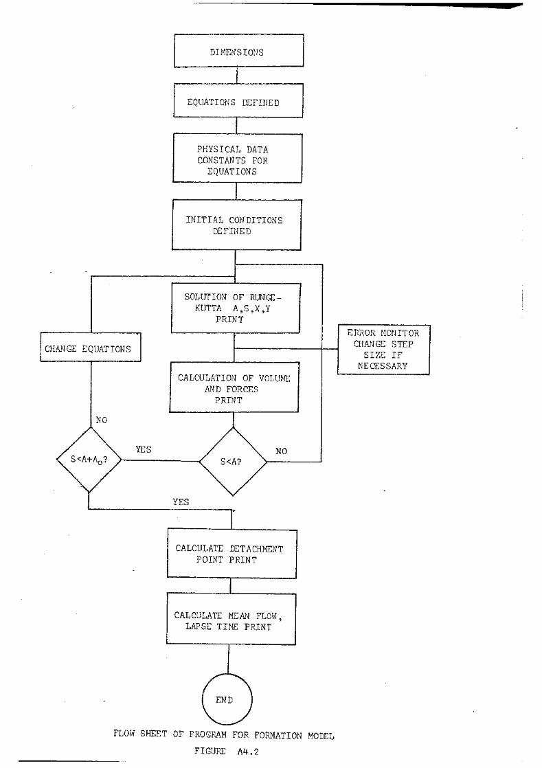
CHANGE EQUATIONS
NO
YES
DIHENSIONS
EQUATIONS DEFINED
PHYSICAL DATA CONSTANTS FOE
EQUATIONS
INITIAL CONDITIONS DEFINED
SOLUTION OF RUNGE-KUTTA A,S,X,Y
CALCULATION OF VOLUME AND FORCES
NO
YES
CALCULATE DETACHMENT POINT PRINT
CALCULATE MEAN FLOH', LAPSE TIME PRINT
FLOH SHEET OF PROGRAM FOR FORHATION MODEL
FIGURE A4. 2
ERROR r10NITOR CHANGE STEP
SIZE IF NECESSARY

FIGURE A4~3
COMPUTER LISTING FOR BUBBLE FORMATION MODEl,
G T H IS t·l 0 0 F. L S I 1-1 U L A T E S G A S t:: U J ~1 l E F C.· R: 1 t\ T I 0 N F f< C r·l .A S I N G L £ C S U £3 r1 E F\G E 0 0 ;:~I F I C ~ • T H E I'; 0 0 E L S E r S J P AN E U U A T I 0 N 0 F t·~ 0 T I 0 N C A N 0 AN E N E R G Y E J U A T I 0 t ~ F U R T H E F 0 F. ,'·II i\1 G ::3 U i: d L E A N 0 S 0 L 1J £ S C T HE S E S I t·1 U L i f\ N E: 0 U 3 LV F 0 f.~ T dE f·: A 0 I I~ L A 1J D V E R T I C A l C 0 11 P 0 N EN T S
C THE PROGRAM WILL P~INT OUT FOk ~ACH INCREM~NT OF TIME THE C R A 0 I LJ S < A ) , T H E D I S T .!!. t' C E 0 F T H E C l ;~ f R C: 0 F T H ~ d U b L L E A l3 0 V E C THE OPIFICE (S), THE Fif\ST .~ND SECO\JO DERIVATIVE~ OF A & S:t C T H E 8 U 13 3 L E V 0 L U ;'1 E < V 0 l J , T H E L I Q LJ I [; I t~ :.: R T I t1 ( A C T ) , T H E I N S T • C FLOW RATE ( FLOR>, T:l::: PRESSURE IN 1 HE GAS CHA~1D~R <PReSS), c C THE PROGRAM IS ALSO UEVISEO TO PRI~T THE INSTANTANEOUS VALUES C OF THE VARIQUS FORCES ACTING ON Tr.E BUJBLE c C T HE P R 0 G R A i'-1 A L :3 J P R. I l·ff T H E A V E~ R J. G E. F L 0 W ~~ A T E (;~A T E > ,
C T H E 0 V E R A L L M E A t i F L 0 W R /~ T E ( A V F L C tJ ) , T H E F R E u U E f\ C Y ( F F: E Q } ,
G THE LAPSE TIM~ <STIME>. c C L .. E C U Y E R .. S V I S C 0 US P f~ E S ~ U i~ E T E ~ M IS INC L U 0 ED C IF YOU rJISH TO f~~t10VE VISCOUS TEf:U DfLETE O.OLt¥-X/A C FROM THE PRGGRAM P~RTICULARLY F~O~ FUNCTION GPHI C REFERENCE: L'ECUYER & MURTHY, N.A.S,A. TN D-2S47 c C T H E U P W t1. f~ 0 t4 0 i1 C N T J M 0 F T H C: G A S I S I N C L U 0 E 0 I N T H I S M 0 0 E L • C IF YOU ~~ISH T 0 f~ t>1 0 Vi THIS S £ T R 2 = 0 c C UNITS: C. G. S. c c ~·~¥~~·¥·~······¥·····~~··~··4····¥··········~)/.············· c C DIMENSION STATEMENTS c
.... _,
.... J
...
.Ji
COMMON PO,R11,R13,R1S,R16,R19,R2U,R21,SIGMA 0It1ENSION ZC4,5) ,t~A(5) ,E<SJ ,C<5) ,QJ<4,5), f(~-,5) 0 I ME N S I 0 ~~ A C 2 U fJ ) , S ( ?. 0 0 > , X ( 2 d ll > , Y { 2 J 0 >
DIMENSION TAC4l ,C<4>
_ FORMAT STATEMENTS
~1 FORMATC• T VOL A S X Y 1 X X Y Y A CC F l 0 W PRESS SA~;
~2 FO~MAT{F7.4,2X,11<E10.2,1X)) 22 FORMAT<13H FLOW ~AfE = ,E10.3)
:6 FORMAT<• SYSTEM PR~SSURE IS •F6Q1• PSI FLOW RATE•F5.1•CC/SEC•) 44 FORMAT<6H [(1)=,E10.2,6H E£2l=,E1f.2,6H EC3l= 7 E10.2,6H EC4J=,E1D.
1} 1 FORMATCF8.4,3X,5(E1D.3,2X)) 5 FORMAT{14H START TIME = ,F7.5,8H SECONDS) 00 FORMAT<• AVERAGE FLOW RAlE = •F10.~~ CC/SEC•> 01 FORf"lAT(~ ORIFICE UIA~1cTt:.~ ""Fifl.?J.' CM •> 02 FORMATe• FREQUENCY •F10.3• BUUBLES/SEC •) 04 FORMAT<• ---------------------------------------------- •>

c c c c c c G c c c c c
.. -··"' ...... -.. ~ --· __ ,. __
FUNCTIONS FO:~ THE VARIOUS P.Ar~.lHiETEf<3 t1RE OEFJI·~ED AS STATEt1E~~T FU>JCTIO~JS W Il H 1 Ht: EXCEPT ION OF GPHI WHICH APPEARS AS A FUNCTION SUdPROGRAM
THE DESIGNATION ··s·· AFTER A FUNCTIGN INDICATES THAT THIS APPLIES WHEN S>A.
VOLUME IN TER11S OF A & S = V~i (A ,S) OR VDS (A) DERIVATIVE OF VOLUME = VBT<A,S,X,YJ OR VOTS<A,X) PRESSUP.E 3fl0H Ot~IFIGC:: = r·<A,S,T) c:< PSCA,T> FUNCTION FOR SURFACE TENSION = FUNC3<A,S> OR FUNC3S<fU SECOND JE~IVATIVE OF S = J?HICA,S,X,Y> OR GPHISCA,S,X) S E. C 0 N 0 D;: R IV A T I V E 0 F A = G P rl I < SUd P i·. U G R A ~1 ) 0 R G PH IS ( A , S , X , Y 9 T )
VBCA,S>=3.1414•(2.JI3.G~A~A~A+A•S~A-S•S•SI3.0)
VBT<A,S, X,Y > =3.1414• <2. !.l•A•A.v-X+2,1 1 ~A•X•S+A-r·J~-¥-Y-S•S•Y)
P<A,S,T> = CPCl-R19~ CV,j <A,S>-r<20-t)4T) > -\l~U.2
FUNC3CA,S>=2.0~SIG~A~(3.0~A+S)/{3.J-\lA¥A+Z.O•A¥S-S~S)
Q PH I (A, S , X, Y) = ~15 + V a r t A , S , X, Y) IV FJ < .4, S > >j{ ( R 16 .!,< V J T {A , S , X , Y)- Y) V8S(A)=4./3.~3.141~~A¥A~A
VBTS<A,X>=12.SbS6~A~A•X
PS CA ,T> = ( PO-R19~ <VJS (A) -172J-LJJ;.T) > ~K12 'FUNC3~<A>=2eO¥SIGMA/A QPHIS<A,X,Y>=R15+(VdTS(A,Xl)~~2•R16/V8S<A>-VGT3(A,X)•Y/V8S(A)
G PH I S ( A , S , X , Y , T ) = ( P S < J.\ , T > + ~ 11 ~ S- P .t 2 -v- F U N C 3 S ( A > +'~ 13 J;C. ( V t3 T S ( A 9 X ) ) .~t- .If 2 .. 1.~A•X~X-R21•i.5~X¥X-O.U4•X/A)/(4.•A•A+R21•A>
KCOUNT=i
PHYSICAL DATA ORIFICE DIA COO> ,ORifiCE RADIUS (.£10) ,ORIFICE COEFFICIENT < 0 R K ) , C H A M B E R V J L ( V C ) , S P E E U S 0 U t Jl1 ( C 0 > , L I Q • 0 EN S I T Y C 0 L ) 9 C R 0 S S S E C T • A R E. A 0 F C 0 l U ~~ i ~ { A RE A ) , P 0 0 L 0 E P T H ( H P 0 0 L ) •
00=0.15875 A0=0.5¥00 ORK=0.0214 VG=37S.O C0=2668t+. 5 DL=i.G AREA =81. 5 HPOOL=5.08 GC=981
CONSTANTS FOR GILL 1·100IFICATlON TO RUNGE-KUTTA.
TEt~P=SQRT <O, 5} AA<2>=0o5 . AAC3)=1.u-TE~1P
AA(L~}=1. 0+1 EMP AAC5)=is016.0 B C 2 > =2, D 8(3)=1.0 £3(4)=1.0 8(5)=2o0 C ( 2} =C. 5 C < 3 > = 1. tl - T E ~! P C{4>=1.0+TEHP CC5>=C,.5
P R F S ~ lJ P F A N n F L 0 ~~ R A T ;:- C H 0 Sf. N T 0 V A R Y F R 0 t-( A H1 0 S PH E R I C

G c
c c c c
c
c
PSI=O.O DO 25 I2=1, 6 Q=5.D 00 24 Il=1, 7
s CC/SEC TO 30 CC/SEC
PROPEKTY VARI~TIO;,J DENSITY <UG> ANU SURFACE fENSION <SIGt1A) WITH P~ES3U~~c.
S I G H A= 7 2 .. 0 ~ < 1 • iJ- n • 1 :3 ~PSI I 2 g ,f • fi ) OG =O.OQ183+G.QJJ1~24•PSI OK=ORK/S QRT ( JG) PO=Z.C>~-SIGM.A/t\0 DLG= Dl- [l G
. 0 t1= 0 G +(I • 6 9 ~ 0 L
WKITEC6,26) PSI,Q
C CONSTANT FOR THE FUNCTIONS c R1=0LG-ii-GC R2=4.C¥OGJ<3.141G•oo•uo> R3=3 .141f)•oo•srG,1t\ R6=0l-\-GG•AREA R?=ARE.CJ. R8=AREA•(4,¥~2/C3.1416•00 4D0>-1./CK/0~) R9=0L•H?OOL R18=RCJ¥3 G 1416 R11=R6/R18 R12=R7/R18 R13=-ARE4/0K/OK/R13 R15= P1/0 i''l R16=R2/0N R17:: R3/0 f'l f:~19=CO¥C 0 •OG/ VC R20=VM(AO,O.O> R21=AREA/HPOOL/3.1~16 K=1
H=Oo001
INITIAL THiE INCREi·lEiH IS SET AT D.0C1 SECONDS THIS WILL VARY T H ~ 0 UGH 0 U T T HE R U "4 0 E P E ~" 0 I N G 0 I\ T H t E R .:~ 0 R A T E A C H S T E P
INITIAL STARTING CONDITIONS
FLOW=O.:) T=OaO A (1) =AO SC1>=D.O x· < 1' =c. o Y(1)=0,Q
r~RITE<6,101> DO wqrTE<o,41>
N U ~1 ERIC A l HE T H 8 J S c E R A L S T 0 I~ AN 0 W I l F V 0 l U ME 1 GILL MODIFICATION TO RUNGE KUTTA
Z CI, J) T U:Po RA R'( STU O:AGt FOi<. RUNGE -KUTT A CALCULATIONS
7(1 .. 1 }::::(\ l1l

..... ,.J
..... -...... -
...... ----_,
-J
..... _,
·---J-1 ,,, __ Z(2:} :d=S \1) Z<3,1.)=X{1) Z!4,1}='r'<1> N=2 DO 50 I= 1., 4
50 QQ (I , l) = 0 s fJ M=1
51 J=1. T=T+ H
52 COi'H It~UE F<1.,J)=Z<3,J).l;tf-i F!2,.J)=Z <4,J)Jt.H IFCHc-EJJ,.G} GO TO 1~) FC3,JJ=GPHI<ZC1,J) ,lC:::,J> ,ZC3,J) JZ<4,J) ,T,PSI,Q>•H f(4'iJ)=QPHI (ZCi,J) ,l C2,..;) ,z<.3,J) ,2(4,J) > ~H
GO TO 9 10 FC4,J)=QPHIS<Zii,J},l(3,J},Z(~,J))<-H.
F<3,J)=GPHIS<Z£1,J) ,l.(2,J> ,Z<3,J> ,l{'+,J) ,T>~H 9 ._CONTINUE
J=J+i DO 53 I=1,4 ZCI,J>=Z<I,J-1)+(AACJ> 4 CFli,J-1)-G(J)•QQCI,J-1) )) .
53 Q Q { I , J ) = 0 Q ( I , J -1 ) + 3 • G ~-- ( A A < J > • < F ( J , ,J- 1 ) - u ( J ) ~ G Q ( I y J - 1 ) > ) - C < J ) ¥ r < I , · 1-1)
IFL.J-?) 52,55,55
STORE FINAL CONDITIONS
55 A{N)=Z<1,5> SCN}=ZC2,5) X<N>=Z<3,5) Yon =Z < 4, 5 >
ERROR MONITOR EVERY FOURTH STEP
IFCM.EQ.O> GO TO 46 IF<K.EJe 4) GO TO 45 K=K+1
46 CONT IIJUE
PRINT A,S,X,Y CALCUL~TION OF THE VARIOUS FORCES INVOLVED
PROGRAM TRANSFER DEPENDING IF S>A I.E M=U
CONST1=F<3,4)/H CONST2=F(4,4)/rl IF0·1.EQ. 0) GO TO 2Q
110 COt·H It,:UE ST=FUNC3(A(~·n ,S(N)) FLOF=VBT (A(N) ,S<N> ,X {N) ,Y OJ)> FLOH=FLOW+FLQR!f.H TE~IP=V3T(A{N),S(N),X(N) ,Y(N) )Jt..ll-2 v o L == v t: < A on , s <: n ' S A= 2 c ~ 3 ., 14 1 6 -\t ( A ( tO "'" A < N ) + S ( N ) .li' S ( N ) ) PRES S=P (A<~~) , S ('·I) , T) I t-:.12 R =X ( N) -t· X ( t~) .!!-2 • ~ ( 2. 11> -~ { ~J) + S (;~) ) t Lr e ~A {f~ ) ¥X ( N ) ),.. y ( t~) R A = Q P H I < i\ < N ) , S ( t·~ ) , X ( t l} , Y { t'l > )' ~ ( A < i ~ ) lf [l. ( N ) - S ( 1\1 ) .!;' S ( N } ) F~ 8= G PH I ( A HJ> , S ( 'n , X {t d , Y ( N } , T , P S I ~ Q ) RC=-2.-v-s (Nl .v-yun .!!-Y(NJ A. C C = 3 • 14 16 -\t ( R + RA + R;J Jf < 2 • ~A { N) ~A (I J ) + 2. ¥-A ( N } >~- S ( N ) ) +f.~ C) TERM=CL•<ACNJ•R3+1.5~X(Nl•X{~)) GO T 021
?0 F10P=\!dTS!A{tJ~ .. X!Nll

·--· .... -·-····~··~,··- •""
F l 0 ~'l = F L 0 ~·J + F L 0 r·t ;;. H V 0 L:.: V hS ( A C!~ ) > sA:: 4 (J )/. 3. 1 L~ j_ 6 .If. A ( ~~ ) ~ t\ ( ~~ ) . TEt-'JP=VBT S <A ( f·U , X ( N)) ~~·z S T = F lHlC 3 S (A on >
PRES S = P S ( A ( i~ ) , T ) I R 1 2 A c c = 12 • 5 s ~4 '!- ~~ < N > ~ < 2 • l,' x < h > )/. x < N > +A ( N} .If. c;? HI s <A < tJ > , s < N) , x < N > , Y ( r ~ ) , T > >
T E R ~~: :: r L l,' ( A ( f D ~ G P H I S ( f:. 0~ ) , S UJJ , X ( N ) , Y { r n , T l + 1. • :..; !;( X ( N ) ¥ X ( N } } 21 CONT ItiUE
HEAO=GC-\1-S(N) ORP=TEMP/OK/OK BUOY=VOL ¥ Ri Gt101'1 =T Er·! P ~R 2 ACT=R9/R7•ACC+TERM I F ( K c 0 J N T - s ) 3 3 ' J L~ ' 3 Lt
34 · KCOUNT=O
... _,
IF YOU WISH TU PRINT FORCES AT EACH STEP REMOVE C NEXT CARD W R I T E l 6 , 4 2 ) T 1 V 0 L , A ( f ·1 ) , S ( N ) , H t. A D , u K P , U U 0 Y , G M 0 f1 , S T , A C T , F L 0 F<. 1 P i~ E S S
\~RITE<6,42>T,VOL,ACU ,S<h) ,X<i~) ,Y 00 ,COtlSTi,COi~Src:,lJ.CT ,FLOF:,PPESS iS A
;3 CONTINUE DO ?G I=1,4 QQ<I,1>=QQCI,5)
56 Z <I , 1 > = Z < I, 5 >
IF<M.EQ.O} GO T011 IF<S<N>,GT.A(N}) GO TO 12
TEST IF S= A 3RANGH IF SATISFIED TEST IF S > AtAO STOP IF SATISFilU <OETACHMENT>
TEST IF INCREMENTS GREATER THAN FIXED NUMUER (200) STOP IF NU~M8ER EXCElGEO
15 CONTINUE 13 N=N+ 1
KCOUIH = KCOUNT+i IF<N~~GT.2Q0) GO TO 25 GO T 0 51
11 OIST=A<Nl+AO JFCS<N>.GT.~)I3T> GO TO ?7 GO T013
12 M=O
INTERPOLATION TO FIND vJHEf~E S =A
C N = { S ( N- 1 } - A n~ -1 ) ) I ( L\ ( N ) - A Ci J -1 ) - S ( N ) ~- S ( N - 1 J ) T=T-H+CN-\1-H A ( N) = t\ ( N - 1 ) + C N ~ < A ( i~ ) - A ( N - 1 ) ) S ( N ) = S ( ~~ - 1 ) + C N lJ. ( .:i ( N ) - S ( N- 1 ) ) X ( N) :::: X ( N - 1 ) + C N ~ ( X OJ/ - X ( N - 1 ) ) Y(N)=Y<N-1) +CN'>L{Y(N) -Y(N-1)) Z<1,1)::.D..(t\) Z<2,1>=-S (N) ZC3,1)=X (N> Z<4, i) =Y <N> WRITE.<6,31>T,VOL,A(N) ,S(N) ,X<N) ,Y<N>
3 CONT It~UE 00 99 I=1,4
99 OQCI,i)=U.O r;n rn 1:::\

98 CONTIHUE c c ··~4······444·~·········*·'·~~······¥·······~···~······*······ (' \.1
c C R E FE R E f'J C E : l A P I 0 U S .~ S E I N F C: L D • Ill~ U >1 E k I C A l S 0 l U T I 0 N 0 F G 0 R 0 It; A :~ y 0 • E ••• s ' A c f'\ [) L ~11 c p R E s s ' 1 3 7 1 ' p 7 6 G
C T RUN CAT I 0 N EFRO~. i'·l01'~ 1TG P
c 45 K=1
TM1=T-H TM2= Tf·11- H rrf3= rr·12- H T A ( 1) = ( 3 3 • ,_A ( N > + 2 4. ¥ A ( IJ -1) -57. 4 A ( r .. - 2) - H 4 ( 10 • • X ( N) +57. • X ( N- 1) + c! f.t .• ~
1(N-2>-XCN-3}})/91.J T A ( 2) = ( 3 3 • • S ( N) + 2 4 • • S ( t~ -1) -5 '7 • • S ( t 1-2 ) -H • { 1 0 • • Y ( N ) +57 o ~ Y ( N -1) + 2 4 • ll-
i(N-2)-Y(N-3)))/90.~
IF 01. EQ. 0) GU TO 2'3 f31= G PH I ( A ( N) , S { N) , X ( N) , Y ( N) , T, PSI , Q) 8 2 = G PH l ( A ( N - 1 } , S { N - 1 } , X { ~ ~ - 1 ) , Y < ~~ - 1 ) , T M 1 , P S I , Q ) 8 3 = G PH I ( t\ ( N - 2 ) , S ( N- 2 ) , X < 1'-l- 2 ) , Y ( U - 2 ) , T t-12 , P S I , Q }
f. 84=GPHI<A CN-·3) ,SCN-3) ,X(i·-1-3) ,Y(iJ-~) ,Tt·13,PSI,Q> CON=33.•XCN>+24.•X(N-1)-57.•XCN-2) T A ( 3 ) ::: { C 0 N- H >~- ( 1 0 • :.~ a 1 + 57 • ll- iJ 2 + 2lt .• v. L! 3- f3 4 ) > I g f1 • C 1 = Q PH I (A 0~) , S en , X. { N} , Y ( N > ) G2=QPHI(,fl.0~-1) ,so~-1> ,X<N-1> ,YCd-1)) C 3= Q PH I { A ( N- 2 > , 'S { N- 2 ) , X C N- 2) , Y ( N- 2 > ) C 4 = Q PH I ( A HJ - 3 ) , S ( N - 3 ) , X t N ~ 3 ) , Y n~ - 3 ) ) CON={33a •Y(N) +2[t.·'~-Y CN-1.) -5/.L~Y CN-2) > T A < 4 > = C C 0 N- H -v- < 1 J • )/. C 1 +57. • C 2 ._ 2 4 • -v- C 3- C 4 > > /9 0 •
( GO TO 30 f. 29 Di=GPHIS<AOn,S(N),X(NJ,YCH,TJ ( 0 2 = G PH I S ( A ( N- 1 ) , S < N ·~ 1 } , X ( N- 1 ) , Y ( N - 1 ) , T t11 ) ( 0 3 = G PH IS < A ( N- 2) , S ( N- 2) 1 X ( 1\-2 ) , Y < N- 2) , T t12)
04=GPHIS (A(N ... 3) ,S (;~-3) ,X (N-3) ,Y(I,J-3) ,TM3> CON=33.•XCN)+24.•XCN-1)-57,•X<N-2) T A ( 3 > = < C 0 N- H ¥ ( 1 0 • 11- 0 1 t S 7 • ¥ 0 2 + 2 4 • .v. 0 :::- 0 4) > I 9 0 • T A ( 4 ) = ( 3 3 • • Y ( N ) + 2 4 • -'~- Y ( N- 1 } - S 7 • ¥ Y ( N- 2 ) - H • ( 1 0 • )/. Q P H I S ( A ( N ) , X ( tJ ) ~ Y ( N )
1 +57 • -¥- QP H IS ( A ( N -1 ) , X { N -1 ) , Y ( N -1 ) } + 2Lt • • U.P H I S ( A < N- 2 ) , X { N- 2 ) i· Y ( N- 2) ) ... · 2PHIS(A(N-3) ,X(,'-J-3),YCN-3)))J /90.
30 E(1l=TA<1l/ACN>•100, E C 2} =T A< 2) IS en •1 iJ '], E(3J=TA<3JIX<N>•1JJ. E(Lf.) =TA(4)/Y{N)lf1(;u;~ 0 IF<ABS<E£3)) .LT.!J.1) H=2,8-\'-rl DO 27 I0=1,4 IF<ABS(E(IQ)),GT.i.O) GO TO ze
27 CONTINUE
c
GO T 0 46 28 CONTitlUE
WRITE<6,44) <E<I> ,I=1,4> H=0.5•H N=N-3 GO T 0 55
c ~~~~·~~~~·~··~~·~·~···~~~·~·~~···.v-·J/.~···~···11-··~~~···~········· c G FINAL DETACHMENT CONDiliONS SY INTERPOLATION c
57 CONI INUE CM::cs<N-1>-ACN-1>-AO)/(A{N)-A(N-1>-S<N> +S CN ... i> >
T =T- H+ C t1• H A { N ) =A ( N -1 ) + C ~1 -v- ( A U-1 ) - A ( N - 1 ) ) S ( N ) = S ( N - 1 ) + C ~1 >~- ( S ( N ) - S { ~~ - 1 ) ) XU~> =X(N-1) +Ct1•CXCn -X <t~-1)) Y { N ) = Y { N - j } + C t1 ¥ { Y OJ ) ..,. Y { N ~· 1. ) )

c \~ R I T E { 6 , ~ jJ r , V 0 L , A ( r~ > :~ S C !\ > , X C I d Sl Y on
P V 0 = P S C A < t·~ ) , T > I R.i 2 WRITECS 1 2744)PO,PVU
2744 FORI",AT(JJ. STA~:T PRESSURE IS.V.E1.C .• 2)/. lJETf\Cf-lt·iFNT PRf~SSURE.IfE10c2)
RA TE=FLO WIT ~JRITEt6,22) RATE
c C LAPSE TIME CALCULATION c
S T I 1'1 E = ( P 0 - P V D ) I;~ 1 9 I,~ I F ( S T I !1 E " G T • i1 • D II Lir~ 1 ) G 0 T 0 3 6 STIME=O.J
36 WRITEC6,35>STIME A V F L 0 W = V 0 L I { T t S T I~~;::)
·t.U~ITEC6,1DO> .ll.VFLOYJ O=Q+5.0 FREQ=1./CT+STIME)
"HRITE<6,102> FREQ rJ RITE ( 6 t 1 0 4 >
24 CONTINUE
c
PSI=PSI+50.0 25 CONTINUE
CALL EXIT END FUNCTION GPHI<A,S,X,Y,T,PSI,Q) COMMON PO,R11,~13,~15,R16,R19,R20,~21,SIGMA V=3.141fi~C0.666•A1J.A~~+A¥A~s-s~s~S/3.)
VD=3.1416~C2o~A•A~X+2o•A~x•S+A•A•Y-S•S•Y>
P R = < P 0- R 1 9 >.1 < V - i~ 2 Q - tj_ * T .) ) ~ f?. 21 FS=2.~SIGMA~<3.•A+SJ/C3.•A*A+2. 4 A•s-s~s>
QP=R1S+VU/V~<R1S~VD-YJ
TEMP=-2.~x~x 4 <2.•A+SJ-4.~A~X~Y+2.•s~Y~Y-QP•<A•A-S¥S}
TEMP1=PR+R11 4 S-R21•FS+R13•Vu•vo GPHI=(TEMP1+TEMP-R21~1.5•X•X-le04¥X/Al/(2.~A•A+2.•A•S+R21•A>
RETURN END

ORIFICE 0 I A METER • , .. ~ • ._ ~ \.,.1' • --...; v v, ....J '- v
.3175000 Ct1 T VOL A s X_- y XX .. ,YY - -
t-< >< tf.) ~ < f-3 .0045 1. a 2 E -0 2 1.63=:-01 1.35E-02 2e68E+OO 5e5<3E+DO 1.08E+03 8.99E+02 0 • 0 070 1.38E-02 1.74'::-1)1 2.97E-02 6~o15E+OO ?.16E+OO 1.54E+03 3A72E:+U2 t-t
• 0 095 2.10E-02 1.94~-01 4.83E-02 1.02E+01 7.61E+OO 1.52E+03 3o55E+01 II II il II II II • 012 0 3.39E-02 2.24E-01 6.73E-02 1.~6E+01 7.57E+OO 1.G9E+03 -3.14E+01
• 0145 5.51E-02 2 • 61 :_::- 0 1 B. 62E- 02 1o57E+01 7.58E+OO 4.74E+02 5.34E+01 Clh Q • c;
~ g: 1-3 • 0185 1.09E-01 3.zs:::-o1 1.1BE- 01 1.5BE+01 8.19E+OO -Y..41E+02 2.52Et-02 !..J· ~· om a "0235 2.06£-01 3.972:-01 1,63E-01 1.23E+01 1.00E+01 -8.82E+02 4.57E+02 1-i c+ cr' o' (!)
4~ I-' I-' .0285 3.15E-01 4. 48 E- 01 2.19E-01 8.32E+OO 1.27E+01 -7.38E+02 5.95E+02 (!) Cl) -~· 0 Cll .• 0 33 5 4.20E-01 4.82~-01 2.90E-01 5. LJ-5E+O 0 1.59E+01 -4.buE+02 6. B 8 E ;- fJ 2 o ro !:tl < ro ro Pl 0 () • 0385 5.1SE-O 1 5.05C:-D1 J.78E-01 3.98E+OU 1.95E+D1 -1.79E+02 ?.56Et02 0 P~ I-' 0
~ t-b ....... g I:S • 0435 6.00E-01 5.24E-Oi 4.8SE-Oi 3.90£ ... 00 2.34E+01 9.81E+01 8.12E+02 p j:lJ 0 Cll Cl) m ~0454 6. 3 0 9E- 01 5.317E-01 5.317E-01 4.231E+OO 2.498E+01 Cl) -l:"i I:S - ......... • 0484 6. 7 7 E-0 1 5.45~-01 6.10E-01 4.38E+OO 2.74E+01 -9.60£+00 7.67t:+D2 t:r::f c+ (') (')
~ a a .0522 7. 443E- 01 5.614E-01 7.202::-01 4.336E+OO 3.021E+01 '7:1 0 ro ............ w H ~ ............ START PRESSURE IS 9.07E~02 DETACHMENT PRESSURE· 1.76E+02 ~ ::7 ~ 0 FLOW RATE = 1. 43 2 E +0 1 t;::J 8 a START TIME = .G2105 SECONDS > ~ AVERAGE FLOW RATE = 10.1583 CC/SEC .:::-. !:t1 FREQUENCY 13.&47 3U8BLES/SEC .:::- ~
~ ~ ;g t:tj f; ~ ~ ----------------------------------------------t-' t-l I?=J 0 0 ACC FLOW PRESS SA 1-3 (I) ::e:: Cf.l Cf.l
II II II II II If 2.06E+02 9.47E-01 1.06E+03 1.68E-01 tf.) 0 H !;f ~=><=
3.59E+02 2.03E+OO 1.13E+03 1a95E-Q1 ~ ~ I:S 5.05[+02 3.8SE+OO 1.19E+03 2.52E-01 til Cll ·(p I-f) c+ ~ 6.03E+02 6.68E.+OO 1.24-E+D3 3.Lt4E-01 p:l 0 P' c+ () ::r 1:$ ....... 5.9UE+02 1.04E+01 1.2SE+D3 4.7SE-01 ro ! c+ Pl
i1 fD I-' 3.16E+02 1.b7E+01 1.20E+03 7.51E-01 :::1
(p Cl) c+ -9.67E+01 2.13E+01 1.04E+03 1.,15E+OO ro 'i 0 ro Pl ~ 1-i -2.42E+02 2.17E+01 8.32E+02 1.56E+OO zy Cll a
m -2.05E+02 2.01£+01 6.41E+J2 ie99E+OO (p 1-:!:j rn I-' -9.80E+01 1.8UE+01 4.83E+02 2.50E+OO rn 0
ti ~ 4.30E+01 1~58E+01 3.63E+02 3.21E+OO ro !:tl
~ 3.84E+01 1.63E+01 2e66E+02 3.73E+OO ro

111.
APPEI'IDIX 5 .
.f..~ o 1 The Effect of P:r:,essure on the Behaviour of Gas Bubbles
E9rmed at a Single Submerged Orifice. R.D. LaNauze
and I.J. Harris. VDI - Berichte Nr 182, 1972 page 31.
"Joint Meeting on Bubbles and Foams".
A5. 2 On a f\1odel for the Format ion of' Gas Bubbles at a Single
Submerged Orifice under Constant Pressure Conditions.
R .D. LaNauze and I .J. Harris. Chern. Eng. Science.
Accepted for public~tion 22nd February, 1972.

VDI-Belichte Nr. 182, 1972
DK 532.58:532.529.6:532.525
The Effect of Pressure on the Behaviour of Gas Bubbles Formed at a Single Submerged Orifice
R.D. La Nauze and Dr. I. J. Harris*)
Summary
Bubble formation under constant pressure conditions has been studied for varying system pressures. The importance and the effect of gas properties, in particular the gas mornentum, on the behaviour of the bubbles formed are discussed. At high pressures the gas bubbling through the liquid is more likely to fonn continuous clzaills. An available two-stage mechanism of bubble fonnation has been adapted to include gas properties and gas momenturn. The model is in good agreement for low pressures but becomes unsatisfactory at high pressures because of coalescence at tlze orifice.
Kurzfassung Vnter versclziedenen Systemdriicken ist die Blasenbildzmg bei konstantem Drnck untersucht worden. Die Bedeutung und der Einj1uj3 der Gaseigensclzaften, besonders die Bewegu.n;;sgr6j3e des Gases, m~f das Verhalten der gebi/deten Blasen werden diskutiert. Bei Jzohen Driicken ist die kontinuierliclze Kettenbi/dung von Gasbltischen in der Fliissigkeit wahrscheinliclzer. Ein schon vorlzandener z~veistufiger Blasenbildungsmechanismus ist angepaj3t worden, um die Gaseigensclzaften u.nd die Gasbewegungsgr6j3e einzurechnen. Bci niedrigen Driickcn gilt dieses Modell mit ausreichender Ubereinstimmung, es wird aber bei lzohen Driicken unzufriedqnstellend, wei! die Blasen sich dann bei der Diise verschmelzen.
Introduction
The literature on gas bubble formation and coalescence in liquid systems has been reviewed by Jackson [ 1 .1. More recently Kumar and co-workers [ 2"
4 1 have presented work to explain some of the existing discrepancies.
to 2,4 X 10⁶ N/m2 gauge and flow-rates from 5 X 1 o-6 to 15 x 1 o-6 M3 /s at system conditions. This range of pressures results in a change in density ratio of liquid: gas of 500/1 at atmospheric to 20/1 at 2,4 x 10⁶ N/m2 gauge corresponding to a. mass flow-rate range of 6,5 x 10⁻⁶ kg/s to 6,75 x 10⁻⁴ kg/s.
Development of the Model
31
A limitation of a great number of these studies has been the wide use of the air/water system and the almost exclusive use of system pressures ncar atmospheric. In many practical situations one or both phases have properties differing markedly from those ofthe air/water system. An exception is the work of Klingl 5l who, in a paper on the dynamics of bubble formation under pressure, points out that gas-entrainment devices which were tested at normal pressures possess quite different operating characteristics at higher pressures, using the same volumetric flow-rate at system conditions. With the increasing usc of high-pressure reactors, particularly those involving the reaction of organic liquids with a gas, there is a need to investigate the effect of gas properties on bubble behaviour.
Two distinct situations for bubble formation were first pointed out by Davidson and Schiiled6 ][ 71, namely 'constant flow' conditions and 'constant pressure' conditions. ln the latter case bubbles are formed with pressure in the gas chamber below the orifice maintained constant. This case is of greater practical importance than the 'constant flow' case and has been used exclusively in this investigation. In 'constant pressure' bubbling the flow rate varies as the bubble is formed, making the equations governing the motion of the bubble more complex.
It is the purpose of this paper to report some results of a study on the behaviour of gas bubbles directed at systems other than air/water at various pressures. As the system pressure is increased the gas properties become increasingly important. In particular the incr'easing g2.s density and hence the increasing gas momentum must be allowed for in any theoretical model.
Present work The present paper deals with the formation of carbon-dioxide bubbles in water with varying types of orifices for pressures up
*) Mr. La Nauze is a research student in the Department of Chemical Engineering and Dr. I. J. Harris is Acting Professor of Chemical Engineering, both of the University of Melbourne, Australia. '
The model presented extends the concepts of Ramakrishnan et al. f2 l and Satyanarayan eta/. [ 3 l to include the effect of gas properties and the force due to the rate of change of gas momentum through the orifice.
It is assumed that bubble formation takes place in two stages as suggested by Siemes and Kaufmannl8 l. During the first, or expansion stage, the bubble expands while its base remains attached to the orifice. In the ~econd, or detachment, stage the base of the bubble moves away from the orifice, the bubble itself being connected to the orifice through a neck of gas. Photographic studies as part of this work have verified this picture of formation.
Further the model assumes:
~ The bubble is spherical throughout formation.
-

32
~ Circulation of the liquid is negligible, so that the liquid surrounding the orifice is at rest when the bubble starts to form.
~ The motion of the bubble is not affected by the presence
of another bubble immediately above it.
.,... Kinetic energy of the liquid dispersed by the bubble may be accounted for in the virtual mass of a sphere moving perpendicular to a waul 6 1 .
Variation of volumetric flow-rate through an orifice can be expressed by an orifice equation[ 9 1 , viz:**
Q = CoYAo ;:;;;;;;; (I) p J~
For any particular orifice, and assuming that the effective discharge area of gas "into the liquid is the same for all gas densities and equal to the orifice area, then,
Q =..!.__ xVEP Vi)
(2)
~nd hence taking the pressure drop as suggested by Davidson and Schiller[ 6 1:
Q = dV = _L/ rpt -pLgh + PLgr- 2a] tj2 (3) dt p 1 2 ~ r
where K is the orifice coefficient determined with the gas on either side of the orifice at the flow-rate, Q, and is assumed to be the same with the gas bubbling into the liquid.
During the first stage the bubble expands with its base attached to the orifice. The upward force caused by buoyancy has to overcome three resistances; viscous drag, liquid inertia and surface tension. The bubble base remains attached to the orifice until the buoyancy force exceeds the downward forces to mark the end of the first stage. The force balance used by Satyanarayan etaf.[ 3 ] yields:
VE(pL- p) = d(MVE) + rrD0 a + 6rrrEf.l.VE - dtE
Buoyancy Inertial Surface tension Viscous drag Force Force Force
The viscous drag term (Stoke's Law) is valid only for a sphere moving at constant velocity with low Reynold's Number. A more general approach is given by Bird et al. [ 10 1, substitution
(4)
for the viscous drag in this form results in a considerable increase in computational complexity which was not considered justified in the present circumstances, where provision for a gas momentum term must also be made.
Equation (4) assumes, that the gas is supplied continuously at a point source which is always located at the centre of the expandirlg bubble. The term for the inertial forces due to expansion
d(MvE)/dt£, does not include the effect of the rate of change of momentum of the gas as it isblown through the orifice. The force due to the rate of change of gas momentum is Q2 pf A0 [6 1, where Ao is the effective area of the orifice and is assumed equal to the actual orifice area.
In these experiments this force acts in the same direction as the buoyancy force. It thus has the effect, if large, of taking the bubble prematurely from the orifice. In the experiments undertaken at atmospheric pressure Davidson and Schulerl6 l found for a small flow-rate, 1 x 10⁻⁶ m3/s that for p = 1 ,2 kg/m3 the momentum accounted for only 0,5% of the force on the bubble.
**)Symbols are defined under 'List of Symbols'.
VDI-Berichte Nr. 182, 1972
For carbon-dioxide at 2,4 x 10⁶ N/m2, gauge, p = 45,0 kg/m
3
the momentum of the gas contributes about 20% to the upward motion at the same volumetric flow-rate.
The force balance now becomes:
4Q2 p d(MvrJ VE(PL- p) + --:::-- + rrDoa + 6rrrEJ..l.VE (5)
rr002 dtE
Following the development of Satyanarayan et al. (3] by substitut·
ing equation (2) and
drE_dVE 1 dtE- dtE . 4rrrE 2
(6)
d(MvE) = M dvE + V£ 5!M_ dtE dtE dtE
(7)
into equation (5) where the virtual mass,
M = VE(p + l_! pL) 16
(8)
Strictly this value of virtual mass applies only in a completely inviscid liquid and should be regarded here as only giving an order of magnitude of the inertial effect,[t.;,.J.t J (6) (11). This lcaus to:
4Q2 p K2 0 + ~-~PL){l . 2 ) VE(PL- pg)g + --
2- =- --- ~ + PLgq;: - _ _£
rr Do P 4rrr1; 2 IE
11 J
VE fp + RPL\ K2 ~ -).- . (4PrE + 3pLgrE 2
- lOa) 32rr~ rE 6 P
3 "a) t/2 + - JL ,1!:._ ! (P + PLgrE - ::... + rrD0 a 2 pl/2 rE rE
(9)
where P = P1- PLgh
Expressing rE as (3/4rr) 113 VE 113 this is solved by trial for VE, the volume at the end of the expansion stage.
Consideration of the second stage
In the second stage there is a net upward force whjch accelerates the expanding bubble from rest. The bubble is assumed to have detached when it has covered a distance equal to the radius rn, at which point the actual bubble radius is fF.
Newton's second law of motion gives:
d(Mv') . ) QE2
P 6
, D ~ = (VE + QEt) (pL -.p g + Ao - rrrf.l.V -rr oa
(10)
where v' is the velocity of the centre of the bubble and is made up of the velocity of the centre due to expansion and the velo.city with which the bubble base is moving,
that is, v' = v + ~ (11) dt
In solving equation (1 0) RamakrislU1an eta!. [2 1 make a simplification which relies, in part, on the change in radius during the second stage being small. Computation based on the model has justified this assumption. The expressions derived by Ramakrislman et a/.[2 1 have been adapted in the detachment stage to include gas properties and gas momentum, leading to:
rE = B (Vp 2- VE 2
)- _g_(Vp- VE) 2QE(A +I) QEA
3G (V 2/3 V 2/3) __ .:_I _ 2QE(A - 1/3) F - E Q(-A + 1)
(Vp-A +1_ VE-A+l) [~~l) yEA+1_(~)V£A
_ ~~t;J yEA-t/3_ ~A~%) yEA-2/3] (12)
v

roi-Berichte Nr. 182, 1972
.vhere
C ~ 1
/ LD0 a- ~_9E 2 p) (p + ---PL QE) ,~ 1TDo2 ' 16
QE 3~ E =------,..-and G = --:::---:-----
127T(frr)'1/3 2(1n )1/3 (P + :~PL)
Equation (12) is solved by trial for V r.
The computer program developed to solve these equations has be~n tested against the data presented for bubbling at atmospheric pressure by Satyanarayan et al. P land found to be in agreement.
·Experimental
Experimental Apparatus
A schematic flow diagram of the experimental equipment is p~esentcd in Fig. I. Gas was released from cylinders through a h1gh-pressure regulator and was metered by measuring the dif· ferential pressure across a calibrated capillary. The flow-rate was also measured, ns an added check, on the down stream side of the bubble chamber by a wet gas meter.
From gas cylinder
74
1. Capillary 2. Differential Pressure Gauge 3. Needle Valve 4. Differential Flow Controller 5. Liquid Drain Valve 6. Water Inlet Valve 7. Filter 8. Gas Chamber 9. Liquid Outlet Valve 10. Bubble Chamber 11. Manometer 12. Pressure Relief Valve 1 3. Gas Outlet Valve 14. Wet Gas Meter
12
Fig.l. Diagrammatic Layout of the Experimental Apparatus
11
The gas was ir.troduced to the gas chamber below the orifice through a differential flow regulator to ensure a steady flow. This chamber had a volume of 2,3 x 10⁻³ m3
• Hughes and coworkersP2l have pointed out the importance of gas chamber volume on the size of the bubbles formed. The conditions throughout this investigation are in the range in which they have
shown th~ 3chamber volume to have no effect. Kupferberg and
Jameson[ l have recently shown for their work that there wa_; no
3Considerable effect of gas chamber volume above 1 ,5 x
10 m on bubble volume or frequency.
The vessel consisted of a 0,1016m dia x 0,3048m section of he.avy gauge stainless steel, flanged at each end with O,OlSm tluck cover plates. Twb 0,0254m thick observation \vindows were fitted longitudinally. The chamber was pressure tested to 5,17 x 10⁶ N/m2 gauge.
Two different orifices were used, a 1,587 x 10-3 m diameter sharp-edged orifice anrl a 3,175 x 10-3 m diameter square-edoed orifice. The pressure drop across them was measured by a o
manometer made out of nylon tubing capable of withstanding 6.9 x 10⁶ N/m2 gauge.
A Red Lake Laboratories 'Hycam' high-speed camera was used with Kodak Tri-X reversal film at 400 frame/s. A Xenon Sk\V flash was used as front lighting, while 3 Phillips Photo-Flood lamps were used to provide a diffuse back lighting.
Experimental Procedure
Many workers have found that small traces of surface active agents, such as greases, can cause changes in bubble sizes. To eliminate this as much as possible the vessel was cleaned with methanol before beginning a series of runs, dried thorougJtly, then rinsed with the test water. Water used was flltered tap water. Anderson and QuinnP 4 l have pointed out that even tap water may cause slightly differing results from day to day. Consistency of the results indicates that this effect was not marked in the work reported here.
33
To carry out a run the char1l.•er was filled to the required depth of liquid and carbon-dioxide bubbled tluough the orifice. The pressure was then gradually increased keeping the pressure of the gas released from the cylinder at 3,4 x 10⁵ N/rnz greater than the bubble chamber. After sufficient time had elapsed for the liquid to become saturated the bubble stream was photographed while the flow-rate was monitered.
The films were then analysed on a 'Vanguard Motion Analyser' which enabled individual volumes and surface areas to be calculated by assuming that the bubbles were surfaces of revolution about the vertical axis. This method was naturally only applicable to regular shaped bubbles. The more usual means of determining the volume' by dividing the frequency into the volumetric flow-rate was used to check this and found to be consistent, and was used for the irregular shaped bubbles.
Discussion The quantitative effect of increasing the system pressure for a constant volume flow-rate can be seen in Figs 2, 3, and 4. As the pressure of the system is increased the bubbles formed first decrease then increase in volume. At the flow-rates presented here the bubbles form singly at atmospheric pressure, however, at pressures of between 2 x 10⁵
- 4 x 10⁵ N/m2 above atmospheric depending on flow-rate the bubbles start to exhibit 'pair' formation.
The onset of 'pairing' is of significance because the second bubble sucked into the wa.I.;:e of the preceding bubble causes a great deal of tur~ulence in the combined bubble and can cause disintegration. The bubble break-up produces a large number of very small bubbles which cause considerable disturbance to the primary bubble thus enhancing mass transfer. They also provide additional surface which is resident in the system for a long period and which could increase mass transfer in cases where this is accompanied by slow chemical reaction. These smaller bubbles have been investigated by Smith and RennieP 5I P6 l _

J>
r 7 ,. •. ....-,
••
~ ~
-·~
] J
-1 " ;~ i 1
'?i ~.t 'l
~~---~··,-;~·.:n•ttr V "_..;_, _,.)fq·:.· G_ • ~~-~·--·eo:~
-!' ~
-~ ,
1
:: K ]
. - )
J. ""'; ...
{
~ ~
~,
.. _io -.i
~ ~ ~ ~
J.i " ~ ,l.:~l ft'H t $' ;, 'i ! -l' ;p' l • '
t i,:, 4 m A M'{":-~;~ sittfiwt§ .t: ... -...i,._ ..
8
A
B
c
Conditions C02/Saturated Water _ Orifice Diameter, 1 ,58], x 10 3 m Liquid Sea1,5,08 x 10 ~m
Atmospheric Pressure p = 0,183 kg/m3
6,894 x 105 N/m2 gauge p = 14.0 kg/m3
2,068 x 106 N.fm 2 gauge p = 38.6 kg/m.:)
Fig. 2. Gas Bubble Behaviour for Constant Volumetric Flow-Rate of 5 x I0-6 m3fs at the System Conditions
c
w ~
< 9 t., ~ ;:::!. (")
a-(1)
z !"I
00 N
..... \0 .....:) t-.J

r"'":'l""..,.,.,...,...·~--- ""'"" . . .... . ... .,. -.. *'?' ,
[h.
A
r~ -- · · · · ... ~- -- •s•·"l r· -~ i ~-
! [: r r t & t. ~.
~--f· t.-f ~-· t t
8
'i .;;,
Conditions C02/Saturated Water Orifice Diameter, 1,587 x 10-3m Liquid Seal, 5,08 x 10⁻²m
A Atmospheric Pressure p_= 1 ,83 kg/m3
B 1,034 x 106 N/m2 gauge p = 20,2 kg/m3
C 2,068 x 106 N/rn2 gauge p = 38,6 kg/m3
,~
~-~~
fig. 3. Gas Bubble Behaviour for Constant Volumetric Flow-rate of 10 x 10-6 m3fs at the System Conditions
~. . ., '· . -·~ .•.. ~ ·-~ , .... , I ~ f . .-~
l:~ 1.-i:· -rf ~',:
~ f t: ~-
r
~j. • c
c
i-t'
't
~ vf
~;.
1 I
... ·
-~ 1
~ ... ~
~ ,_. ~ (l>
;:J. 0 ::r (II
z !"' -00 __tv -\Q ~ ,N
w Vl
1
1
I

36
Thus the initial increase in pressure increases the surface area/ volume of the bubble, if the volumetric flow-rate is kept constant. Constant volumetric flow-rate implies an increasing mass flow· rate, in practical situations where constant mass flow rates are normally encountered, an increase in pressure could cause a reduction of the surface area/volume ratio.
A point is reached where the bubbles start to form intermittent chains. Chaining at higher pressures becomes even more marked till it has increased to such an extent that discrete bubbles or bubble groups are no longer formed. This streaming would cause a decrease in mass transfer efficiency not only because of a decrease in surface area/volume ratio but also because less of the streaming gas comes into contact with the liquid.
When the bubble detaches from the orifice it leaves behind a smaller bubble from the rupture of the bubble neck. This can be seen in the growth curves Fig. 5 where the bubble volume just prior to detachment is slightly larger than the final detached volume. This secondary bubble may either grow immediately resulting in 'pair' formation or be pushed back resulting in weeping. Kupferberg and JamesonP 3l have pointed out that pair formation occurs when the pressure of the gas chamber is greater than or equal to the pressure behind the detaching bubble. The onset of pair formation here is caused by increased pressure drop across the orifice. From equation (2) it is evident that as the density of the gas is increased by increasing system pressure, the pressure drop across the orifice must also increase to maintain constant flow-rate.
The effect of increased gas momentum causing the forming bubble to leave 'prematurely' from the orifice is demonstrated in Fig. 5. It can be seen clearly that the increased pressure (and hence increased gas density) alters only slightly the growth/ time curve, but terminates the growth at an earlier point.
The onset of streaming is difficult to ascertain. For the conditions reported here it does appear to be a function of mass flow rate CPgQ), however remembering that these results have been obtained for a particular orifice diameter, pool depth and for C0 2 /water further studies are clearly required to find the importance of these other variables. It is intended to pursue this aspect of the work.
Comparison of the shape of theoretical and experimentally determined curves clearly suggests that some other factors are still needed in the model. It was observed that the second bubble of each pair was generally smaller than the first. This is because the pressure in the wake of the first bubble just aftpr detachment is less than that above the orifice P 71 , if at the sa me time the gas chamber pressure is greater than this pairing rapidly occursP 31 P 81. This pressure decrement will cause the release of the forming bubble from the orifice within a shorter time than predicted theoretically. It would be expected then that a model which does not take account of the effect of the preceding bubble, will give volumes which are larger than the average experimental values.
In summary the model works well for flow rates up to 15 x 10-6 m3 /sec at atmospheric pressure but quickly becomes inaccurate at higher pressures. As pointed out above this is not surprising as the model in its present form does not account for pairing or liquid circulation. These inadequacies become more apparent as the pressure is increased and a more rigorous model must be formulated.
Conclusion
At increased system pressures the increased gas momentum has a marked effect on the type of behaviour occuring at single submerged orifices. The onset of streaming at high pressures
0 5 AJO 0 75
--Theoretical
// 8/
VDI-Berichte Nr. 182, 1972
I o/ /
/0
I I I
I ol I
I I
I I
OOL---J----0~·5--~----,~0----~---,.~5--~----~--~~
GAUGE PRESSURE (x 10 6 N/m 2)
Conaitions C02 /Saturated Water _. Orifice Diameter 1 ,587 x 10 .lm Orifice Coefficient, K = 0,0214 Liquid Seal, 5,08 x 10-'lm
Fig. 4. Plot of Avcrag~.: Bubbll' Volume versus Gauge Pressure Showing Experimental Points and Thcorctkal Curve from the f'.lodd
8
Conditions:
Arrow indicates point of detachment
/~o/ ~L
/6. e:.
o Atmospheric pressure
e:. 3·4-47 x 705
N/m2
gauge
o 6·894 x 70 5 N/m 2 gouge
C02/Saturated Water Orifice Diameter, 3,175 x 10-3 m Liquid Seal, 5,08 x 10-'lm Flow-rate (at system pressure), 20 X 1 o·6 m 3 /s
Fig. 5. Experimental Data for Growth of Bubbles versus Time for Different Pressures

VDI-Berichte Nr. 182, 1972
as reported here is a function of volumetric flow-rate and gas density.
The modified model of gas bubble formation holds reasonably well for low system pressures but at elevated pressures the limitations of the assumptions on which the model is based become increasingly apparent.
Acknowledgment The Authors wish to acknowledge assistance from the Australian Research Grants Committee in purchasing equipment.
List of Symbols A = as defined in text A 0 =area of orifice B = as defined in text C = as defined in text C0 =orifice coefficient, defined by equation (1) Do = orifice diameter · E =as defined in text G = as defined in text g =acceleration of gravity h =liquid seal above ori t1ce K =orifice coefficient, defined by equation (2) M =virtual mass of bubble P =P1 -Ptgh P1 ==difference in pressure between gas chamber and bubble
chamber b.P = pressure drop across orifice Q == volumetric flow-rate of gas OE == volumetric flow-rate of gas at end of first stage r ==radius of bubble IE =radius of bubble at end of first stage If .=final radius of bubble t =time tE ==time in first stage V ==volume of bubble VE ==volume of bubble at end of first stage VF = final volume of bubble v =velocity of base of bubble in second stage v, =velocity of centre of bubble in second stage VE =velocity of centre of bubble in first stage Y =expansion factor, defined by equation (1) {3 =ratio of orifice diameter to pipe diameter a == surface tension p = gas density PL =liquid density J1 =viscosity of liquid
References
[1] Jackson, R.: The Chemical Engineer. 178, May (1964) CE 107.
[2] Ramakrislznan, S., R. Kumar, and N. R. Kuloor.: Chern. Engng. Sci. 24 (1969) 731.
(3] Satyanarayan, A., R. Kumar, and N. R. Ku/oor.: Chern. Engng Sci. 24 (1969) 749.
(4] Khurana. A. K., and R. Kumar.: Chern. Engng Sci. 24 (1969) 1711.
[5] Kling, G.: lnt.J. Heat Mass Transfer. 5 (1962) 211. (6] Davidson, J. F., and B."O. G. Schiiler.: Trans. Instn.
Chern. Engrs. 38 ( 1960) 144. (7] Ibid page 335. [8] Siemes, W., and D. F. Kaufmann.: Chern. Engng Sci. 5
(1956) 27.
[9] Perry, J. H. (Ed.): Chemical Engineers' Handbook (Fourth Edition). New York, Toronto, London. MacGraw-Hill Book Company Incorporated (1963).
(10] Bird, R. B., W. E. Stewart, and£. N. Lightfoot.: Transport Phenomena (New York, London: John Wiley & Sons, Inc.)
[11 j .Milnc·Thornson, L. H.-Theoretical Hydrodynamics, 2nd. edition. 1949 (London: Macmillan & Co. Ltd.)
[12) Hughes, R. R., A. E. Handlos, H. D. Evans, andR. L. Maycock.: Chern. Engng Prog. 51 (1955) 557.
[13} Kupferberg, A., and G. J. Jameson.: Trans. Instn of Chern. Engrs. 4 7 {1969) T24 I.
[14 j Anderson J. L., and J. A. Quinn.: Chern. Engng Sci. 25 (1970) 373.
[15] Rennie, J. Chern. Engng Sci. 18 (1963) 641. [16} Rennie, J, and W. Smith.: A.I.Ch.E.-I.Ch.E. Symposium
Series No. 6. p 67. [17] Jameson, G. J., and A. Kup[erberg.: Chern. Engng Sci.
22 {1967) 1053. [18] McCann, D. J. and R. G. H. Prince.: Chern. Engng Sci.
24 (1969) 801.
Discussion
37
W. F. Calus, Loughborough, England:
The bubbling process described by the authors is bound to set up in the liquid phase an oscillating motion. This represents an additional inertial force not taken into account in the development of their model describing the process. A secondary effect of the liquid oscillating motion might be coalescence of the bubbles at the orifice itself. This is an intuitive guess which should be verified by visual observations before acting on it. One would expect that the intensity of oscillations would be dampened at higher pressure on the system and thus one of the causes of coalescence at the orifice cancelled, at least partly.
According to the reasoning the bubble volumes in the low pressure region should be still smaller than those shown in Fig.4 of the paper making the deviation from the predicted values larger. However, the mathematical model is probably not complete, as stated earlier. In addition to this, the authors used surface tension and viscosity values for water at atmospheric pressure. These probably cannot be taken as independent of pressure. At 20 atmospheres viscosity1
) and probably surface tension as well could be significantly different from the atmospheric pressure values.
Dr. T. F. Davidson, Cambridge, England:
I suggest that theory of the kind set out in the paper by La Nauze and Harris could be adapted to explain some of the results given in the preceding paper Vollmilller and Walburg. For example the latter's experiments show, that wiih upward liquid flow, the bubble volume is less than in stagnant liquid, Fig. 5. This reduction in bubble volume is to be expected on the basis of the theory of bubble formation at an orifice; an upward liquid flow must detach the bubble formation at an earlier stage in its fonnation.
Putting the above into quantitative terms, imagine a bubble fanning from a point source of gas in a liquid stream having an upward velocity wF. At timet after the bubble began to form, its centre has moved up a distance
s=wFt (1),
wy being sufficiently large for the bubble acceleration due to buoyancy to be negligible. Assuming the bubble remains spherical, its radius r is given by
4nr3 · (2) -3-=VGt .
1) The properties of Gases and Liquids, R.C. Reid and T.K. Sherwood, McGraw-Hill, 1966.

38
The bubble will detach when r = s, and eliminating t from between equation (1) and (2) gives the diameter at detachment,
-(3 VG) 1/2 da--
7l'WF (3).
The above is obviously a grossly oversimplified argument, but ~ equation (3) gives results which show the same trends as the data of Vollmilller and Walburg. Thus with V G = 0.1 m3/h: when wF = 1 m/s, equation (3) gives d8 == 5.15 mm, and when wF = 18 m/s, da = 1.21 mm, and the corresponding values from Fig. 5 are d8 = 5.5 mm and 0.4 mm. Furthermo~e, equation (3) shows that at constant wF, d8 is proportional to Ya, whereas Fig. 5 shows a lower index on Va; a lower index would be obtained if the acceleration of the bubble due to buoyancy was included in the derivation of a revised form of equation (3).
Prof.Dr.P. Grassmann, Zurich, Schweiz:
Die V crgroBerung der OberfHiche auf Grund der Abweichung von der Kugelform wird meist stark iiberschatzt. Driickt man sie durch die Spharizit&t (Oberl1ache der volumengleichen Kugel/ tatsachliche OberfHiche) aus, so crgeben sich auch bei starker Abwcichung von der Kugelform Werte, die meist nicht wesentlich kleiner sind als 1, z.B. ftlr den Wiirfel 0,81, fUr den Sprechenden 0,45. AuBer in extremen Fail en ist es also durchaus statthaft, mit kugelformigen Blasen zu rechnen.
Der Fall, da£ sich die Dich.te des Dampfes und die der umgebenden Fllissigkcit einander niihern, wurde von U. Grigull, Mlinchen, untersucht, der Dampfblasen von C02 in der Nahe des kritischen Punktes untersuchte und photographierte.
J. C. Lee, Swansea, Wales:
I suggest that Dr. Harris might use a solution of an electrolyte for his bubbling experiments instead of pure water. Electrolytes have a profound effect on coalescence processes occuring on the time scale 0- 1 sec. approx. They do not, however, produce stable foan1s and therefore differ from the usual surface-active class of substances in that electrolytes have little effect on processes occurring on a time scale greater than 10 sec. approx.
Dr. H. Pfeiffer, Winterthur, Schweiz: Welche Form der Blasenkette konnen wir erwarten, wenn die Dichte der Gasblasen so sehr gesteigert wird, daB sie die Grp11enordnung der Dichte der Flussigkeit erreicht?
R G. H. Prince, Sydney, Australia:
The paper refers to work indicating the importance of chamber volume (Refs.l2, 13, 18): Tbis is due to coupling of pressure changes in the bubble and chamber. The relevant factors must then be at least orifice diameter, gas density and gas flow, in addition to volume, and it would seem a considerable simplification to take the volume only as a sufficient indication of the limit "at which the chamber has no effect". In what way has this assumption been tested? At least one would need to check the pressure variations in the chamber, but this would appear not to have been possible with the equipment shown. My experience (Paper Ref.18) w~..~·ld suggest the chamber to remain important well beyond the size used, for much of the experimental range investigated.
Prof.-Dr. J. Szekely, Buffalo, N.Y., USA:
As a rejoinder to Professor Grassmann's comments, I suggested that we were faced with a dilemma in our attempts to make allowances for the fact that the bubbles are not really spherical.
VDI-Berichtc Nr. 182, 1972
If we retain the assumption of sphericity we may generate "exact" solutions through the use of the Navier-Stokes equations. On the other hand, if the non-spherical nature of the bubbles is taken into account we will have to use empirical relationships - if unbearable mathematical complexity is to be avoided.
The problem is then whether to use exact mathematics to describe a not accurately represented physical situation, or to resort to empiricism which in itself may not be accurate.
R.D. La Nauze and Dr. LJ. Harris, Melbourne, Australia:
In essence the paper presented is a preliminary study of an aspect of gas/liquid behaviour which has received little attention to date. The discussion has shown that there are several aspects of the work which require further clarification. In the paper presented some realism and result:mt complexity of the model was sacrificed in ordt!r to obtain comparative simplicity of the mathematical equations.
The authors would like to take the opportunity of adding here further data which was presented with the paper and is relevant to the discussion above.
The results, Fig.4*), were taken from preliminary high speed photographs at 400 frames/ sec. It was assumed that a "bubble'' consisted of irregularly sized jets which disintegrated on rising some distance from the orifice, a picture not unlike that described by Leibson et aJ 1), but with the absence of the large number of very small bubbles. The results of Fig. 4 *) are based on the understanding that a bubble is formed when the gas stream exhibits a complete break at or near the orifice.
Faster motion pictures, up to 2000 frames/ sec., show the inadequacy of this definition. It is clear from these later films that at high system pressures many more bubbles are formed at the orifice than was previously apparant, but because of the greatly increased gas momentum they are immediately coalescing with the p;:-eceeding bubble. These bubbles then form intermittent chain::: of from one to more than six. bubbles. A new criteria for bubble formation was therefore required.
If the idealized picture of fonnation (a) as shown below is continued into a region where the gas momentum is high and the next bubble starts to grow without interruption then the idealized picture would look like (b) as shown below. In a real situation (for instance, Fig. 2c) *) the behaviour is not nearly as clear cut as this, though chains of bubbles and J).ecks were frequently observed.
a)
When this type of formation occurs demarcation between bubbles becomes less distinct and a degree of subjectivity comes into de· ciding when a bubble has actually formed. These guidelines were used:
1) As before, the break in the gas stream signifies the end of a bubble.
2) The formation of a meniscus to accomodate a sharp ch!nge in surface contour at the narrowing of the neck. Tltis meniscus may exist for only a fraction of a second before being ruptered by the succeeding bubble.
1) Leihson, !., E. G. Holcomb, A. G. Cacosco, and J. J. Jacmic: Am. I.Ch. E.JI. 1956, 2, 296.

VDI-Berichte Nr. 182, 1972
3) There are cases where the formation of a meniscus was difficult to detect but this usually occurred where a definite bubble- neck pattern existed.
0,7·70"8-----------------------,
m3
0
C02 / waferr
a 75 ·10-6 m3 s-1
... 10 ·10"6 m3 s-1
o 5· 70" 6 m3 s- 1
Using this criteria the experimental results have been recalculated and are presented above.
Professor Prince suggests that we have not adequately accounted for the effect of coupling between the bubble and gas chamber pressures. The constant pressure assumption was a simplification based on calculating the capacity number, Nc, given by Hughes et al. [12] **)which gave 50> Nc > 5 for all runs. Constant pressure assumed when Nc ~ 1. We have since found from oscilloscope traces superimposed on film bubble formation that pressure fluctuations of between 10 and 20 mm H2 0 occur in the gas chamber similar to those reported by Kupferberg and Jameson 2)justifying Professor Prince's objection. The degree to which this effects the theoretical results has not been worked out. The variation of gas cluimber pressure can be expressed [2] **)as:
20·· C2 p Pc =-r - -V. g [(V- V0 )- Gt].
0 c
But this is difficult to incorporate in the type of "mean" force balance approach given here. An incremental model has been developed, which, it is hoped, will be published elsewhere. The new model incorporates chamber pressure fluctuations and a term to describe the liquid inertia around the bubble. Further it is hoped to incorporate the effect of the liquid phase surface oscillations mentioned by W. F. Calus. From a preliminary examination these would appear to cause a large cyclic variation in gas chamber pressure onto which is superimposed the cyclic variation of the individual bub-
39
bles. The intensity of the oscillations do not appear to be dampened at higher system pressures as suggested, on the contrary, both surface oscillations and coalescence appear to be increased owing to the greatly increased gas momentum.
The assumption of constant viscosity of water up to 20 atm. appears to the .-:uthors to be reasonable. Although under very high pressur~s large increases in liquid viscosity have been noted. Reid and Sherwood3
) point out that water is an anomaly increasing only two fold from 1 to 10,000 atm. The contribution of the viscosity term in the equation is small when compared with the other terms. In fact, various authors [2;7] **)have assumed that gas/water sys· tems behave inviscidly and take 11 = o.
Surface tension at 20 atmospheres pressure has decreased to about 80% of the value at atmospheric prcs:,ure 3
). This could be used in the model to give increased accuracy.
Commenting on the points made by Professor Grassman and Professor Szekely, the authors have found that the assumption of sphericity holds well even for very non-spherical bubbles and that this is preferred over the increased complexity of other shapes were to be considered. Some work of Collins 4
) for extremely high gas velocities where the bubbles were anything but spherical showed that the assumption of sphericity gave reasonable results. This suggests that shape may not be an important consideration, the ratio of the various forces acting being more important. Me Conn and Prinr:e 5
)
point out that there may be some distinction in the shape of bubbles formed at small orifices compared with large orifices. Small orifices following Hayes et al6
) mode] for growth, where the surface of the bubble always touches the perimeter of the orifice rather than the Davidson and SchWer [ 6} **)type model where the bubble grows out along the orifice plate. It is our experience that this appears to make little difference in the final analytical result, again suggesting that shape of a singly formed bubble is not the most important consideration in modelling. However, there still remains the problem of trying to account for the effect of the preceeding bubble and of liquid circulation. Dr. Dm•idson 's approach may b6 useful in attempting to allow for the latter.
2) Kupferberg, A. and G.J. Jameson: Trans. I. Ch. E. 1970,48, T 140.
3) J?_eid. R. C. and T.K. Sherwood: The properties of Gases and Liquids, MacGraw-Hill, 1966.
4) Collins, D. 0.: B. Eng. Thesis, private communication withDr.J.F.Davidson, Cambridge, U.K.
5) McCann, D.J. and R. G. H. Prince: Chern. Eng. Sci., To be published.
6) Hayes, W.B. !II, B. W. Hardy, and C. D. Holland: A. I. Ch. E. Jl. 1959,5,319.
*) Figure numbers refer to the original paper.
**) Reference numbers refer to the original paper.

&7 I
C ES 1 7 1 0- Gal. I.
On a model for the formation of gas bubbles at a single submerged orifice under constant pressure conditions
(First rc:ceired 12 Nore111her 1971; occepred2?. Fcbmury 1972) I
A THEORETIC.\ I model for predicting the volume 0f bubbles formed at a single submcrgetl orifice bubbling undl!r constant pressure conditions has been suggested by Davidson and Schuler[ I. 2] and modified by Satyanarayan ei' a/. [3].
This work presents a model based on Davidson and Schuler's[2) approach but incorporating terms in the gas flow equation to describe the liquid inertia caused hy vertical translation as proposed by Potter [4 I and radial acceleration of liquid immediately surrountling the bubble a'i described by Kupferbcrg and Jameson[5]. The model has been used to predict bubble volumes and mean gas flow rates for the experimental study made by Davidson and Schulcr!2) with significant improvement over the earlier models.
The model considers that the bubhle is formed at a point source in the liquid. Initially, the bubhlc centre is at the point source, the centre of the upper face of the orifice, and its upward motion is determined by a h:llance between buoyancy and inertia. Davidson and Schulcr[2] assumed spherical growth. the model here considers only that spherit.:al segment of the bubble which is above the plane of the orifice.
The sequence of events on which the model is based is shown in Fig. I.
The equation of motion of the bubbJe is: ,...-tv .... ·~
V , d(M.n f.';··-·fl ). v·. ,1 •• 1 I (p-p )g=-d-t-=xp/+16p ( s+,s) . )
where the effect of the kinetic energy is assumed to be accounted for by taking the virtual mass of the bubble [I). r,"',
Davidson and Schuler[! I assume that an orifice equation_., of the form Q = d . .P 1 ·~ can be modified to give the flo\.V into the bubble, viz:-
Q = V= K(P1 -pRh+pgs-2;)'
1:!. G
This equation is derived from a force 'balance over the liquid column from the orifice to the free liquid surface. Davidson and sc'hulcr[ I y.,(2] and Satyanarayan [3) neglected the effect of liquid inertia by taking the right-hand side of Eq. (2) as equal to zero. PotterJ4l shows that this effect. which may be represented hy ph VJA. is of significance v-,•hcn compared with the other forces acting. but dL)CS not explore the consequences of taking it into account.
The term used by Potter(4] describes the inertia caused by the upward translation of the bubble. It is also necessary to consider the effect of the radial acceleration of the liquid immediately surrounding the buhble. Kupferberg and Jameson [5{l6J describe this e1fect, the relevant term being:
I I
p[aa+3/2(t}:J~].
Although this strictly applies to the whole sphere it is assumed in this analysis to be applicable to that portion of the sphere above the orifice and that the reaction or the orifice plate may be neglected.
c:)
Fig. I. The bubble formation sequcn;.::e analysed.
()) ... _...,

The final equation. cxpr~sscd as a pressure halam:~. becomes:
n I \f' I, ( ,· .. , ph V [. .. '/~ . ·• J .., , 1 -- pg 1 -+- pgs -- u ,, - j~ -J- = A- -t fJ . cw + ·' ..: t c.~)- (- J
,/
Static Hydro- Prco.;o.;ttre Pressure I ncrtia Inertia of' pres•nJre static C<lll'-.Cd by lo-;s of liquid liljllid drop i<.1SS .>urface through due to surrounding
tension the translation the bubble. orifice
The volume of tht.: bubble and its derivatives arc:-
for s < o: for s > (t
V = 77 ( 2/3c.x:1 + a~s- .\:1/3)
V = 1T(2o:2i.d- 2m\s + a~s.i -st.O
F ~"' rr ( (x ( 2a2 + ~n .1 l + 2<'1 ~ ( 2n + .I J
+ 4aLi:.i -- 2.1 .i~ +- _;· (at - .\~) )
/ v = 4/37TO::t
r/ = 41Ta2a
and .l?., is obtained hv equating the work done in cxran~;ion to the increase in surfa~c energy, es.;-11 1 = 1rJA
whence /:l/',, = ~<; 1 J£~.; for s < ex Ja~ + 2ns - .1·~
By taking:
Eq. (I J becomes,
and Eq. (2),
= 2rr a
a=x J=y
_\· = 1; (a, s, x, y)
.\· = .1; (n, s, x, y).
for s > a.
(3)
(4)
(5)
(6)
These four first order ditl'crcntial equations (Eqs. 3-6) have been solved simultaneously for c~ • . I. x andy using a 4th order Runge-Kutta ( <. i ill moditicat ion) numerical tct:hnilJLIC for the initial conditions at f '""'(}Of(~= (~0 • I'"" 0, X =c 0, .\' = 0. The detachment criterion was taken as s '"' a+ u 11 to allow for the initial volume at 1 ., 0 of 2/3m~,) 1 •
The results arc compared with those of Davidson and Schukrl21 and Satyan<trayan el o/.[3] in Table I. The theoretical values of the ll1l.'<l!l llow rate rJ and the final volume V have bccn .!:!!"l'iilly reduced from tho-.e prcviou-.ly reported by the indusion uf the terms for the acceleration of the li4uid and the nwre ... t ringcnt gcomct ric rcprescntatiur.. The results from these rnoditicatitlns arc -.igniticantly clos~.:,· to the experimental values. particularly for the larger diameter orifice-;.
In- the origim1l \lurk of Davidson and Sc11ulcr[21 the liquid depth. II. is not c\pliL:itly ~pc..:itlcd. being included in P. However the liquid depths were between 5 and 15 em. Results arc presented rnr It= 5. 10 and 15 em. Taking these extremes docs nut alter the increased accuracy of the results to any great extent. for instance. fur the case P = 877 (gm/cm 'ICC~) given in 1-.-igs. 2 and 3.
forft = 5. I'= 5·54 (} = 73·2
h = 15. ~· = 5·07 Q = 66·2.
The plot of bubble growth. instantaneous llow rate and accclcmtiGn of the bubble. Fig. 3. shows that the acceleration of the liquid column is most marked during the initial stages of formation at whil·h time it has considerable inllucncc on the flow into the huhhle, This is rellected in the growth and flow rate curves. Sub!-.ClJUcntl~r tht! acceleration nt' the liquid column decreases rapidly. pnsses through a minimum and then rises to a smaller muximum. Th<.~ second maximum occurs for the time ut which .r =c.~. The increase in the inertial term" towards the end of the bubhlc growth mav be useful in accounting for the s~cond stngc of growth Jl()Stulilled in tl1c litcraturc!2. 3. 5 j.
The rate of grnwth of the bubble at any particular timt.: is dependent on the relative magniiudes of the fon:cs ucting on the bubble ut that !inte. Ccr,.parison of theory and exp • .:rimcnt ~-<-sed o-1ly nu !~1.; fin•~• ,_•uhblc volu~ncs uocs uot allow one to assess chc instant<ll1Cll\JS for~..:es whercns the U!-.C of an incremental force balance approach gives the magnitudes of these forces at cucb instant during rm·matio~1. The eficct of terms. such as the inertia terms. which have a low rn~an value over the total formation period hut a relatively large cfTect at some stage or the growth is obscured in the mean nr final t'l)r<:e halancc model (31 whkh predicts only flnal bubble volumes. This approach is an umlcsirablc simplitkation in certain cin.:umstanccs. f'nr instance, in the study or mass tmnsfer Juring the bubhle formation period where it is prefcrahlc to know the volume at each point of rime.
In t:onclusion. for the c.xpcrimcntal data of Davidsl)ll and Schulcr[21. the model presented shows cunsiucrab!e improvement over previous models [:2··. 31 in predicting theorctienl huhhlc volume ami rn~:an gas flow rate over a wide ntngc nf' orifice radius and gas flow rute.
Acknowledgement-The authors wish w acknov.·Jedge assistance from the Australian Research Grants Committee.
/)c•[lfi/'IIIIC'IIf r~/'Chl'lltical t:ngineerinR lJ nit•l'J'sity f~(M e/lwume Mcihoume. Austmlia
R. D. Lt\ NAUZE I. .J. HARRIS

Time, sec
Fig. 2. Theoretical curves for mdius, (K (em) unJ distance from ori!it:c, .\(ern) with lime l'or the case n11 = O·lh7 (em) P = H77
(gm/scc!) h =·, 10 (em). .A
E u
ai u c: !;) ·u; C.i
12
001 002 003 004 005 006 007
Time, sec
Fig. 3. Thcoreticul curv7'('for hubble volume, ~· (cm'1),
instantanenus_. flow rate,\ I )(em :/sec) and liquiJ inertia fJhi:tA +JJ (c'tti:'+J((~n for the case n,O·I67 (em) P=877
-· (gm/cmsec!)fl= IO(cfllJ.
.=./. y
/.f) .. \ s 17 c) s. c: I f<.,.AN I
~G o rJ L- '/)
'\l 1 u5 ~· o·t<.
IH\~ IS
FtC. 2.

~ -.--
CES 1710- Gal. 3. End.
NOTATION
A column area no orifice radius
C.l:' buhhle radius --\._a~ I -.t and 2nd derivatives of rx w.r.t. time
-~- acceleration of gravity
2an em
h liquid -;cal K orifice col.'!licient
M virtual rna-;s of the bubble P 1 gauge pre-;sure below the orifice p PI -i._:t:h
D.P pressure drop across the orilke !:l.Prr increase in pressure caused by surface tension ~ instantaneous gas llow rate 0 mean gas tlow rate
.1· distance of centn: of hubhlc above oritlce (I !J.~~·r I stand 2nd derivatives of.1 w.r.t. time
I • 1 t1me v volume or bubble
~·,V I stand 2nd derivatives of V w.r.t. time X ex y .~
p' gas density p liquid density a surt'acc tension
REFERENCES
[I] DAVIDSON .I.. F. and SCHULER B. 0. G .. Tmns.lnst. Chem. En;.:rr}! 196038 144. l21 ibidp.335.
1-
13] SATY.-\NARAYAN A .. KUMAR R. and KULOOR N. R .. Chem. Engng. Sci. 1969 24.749. [4) POTTER 0. E .. Clte111. l:.11g11g Sci. I 96l) 24. 1734. [5) KU PFERBERG A. and .JAMESON G. J.. Tmns.l11stn. Chem. En.SA..I 909 47 T::!41. [6] KUPFERBERCi A. and JAMESON G. J.. Trw1s./nsrn Chem. Engrs 1970 48 Tt40.
/ Table I. Forrnation of air bubbles in water with constant pressure. (T = 72 dyn/cm
. ,/ . . rr I p;·
K p 2cr/au 1 Mean gas tlow rate, Q Bubble volume. V /-cm'i2f g/cm dyn/ Ex pt. Ref. Ref. This work c i •
i Expt. Ref. Ref. This work gmL2 sec2 em~ 121 [3] h=5 h= 10 h = 15 1 [2) [3] h=5 h ::;~ 10 h :::;; 15
I ____ .. ________
0·298 1·9 951 * 968 . 3::! 67 65·5 44·4 42·0 i
40·6 i 2·3 3·5 3·29 3·06 2·95 2·83 0·298 1·9 1118 lJt'JH 45 70 61.Hl 51·6 50·3 49·0 I 2·9 3·8 3·52 3·55 3·46 3·42 0·298 1·9 1323 968 61 76 73·2 58·l) 57·5 56·2! 3·4 4·2 3·78 4·02 3·95 3·89 0·374 3·06 779 771 33 102 86·4 63·6 59·4 56·9 3·2 6·1 5·89 4·88 4·59 4·31 0·374 3·06 877 771 47 105 89·7 73·2 68·8 66·2 4·1 6·4 6·13 5·54 5·32 5·07 0·374 3·06 1024 771 60 II:! 93·9 83·8 79·2 76·4 . 4·5 6·9 6·47 6·26 6·09 5·78 0·412 3·82 734 698 30 124 109·0 80·9 73·4 69·9 4·3 7·8 7·88 6·37 5·85 5·43 Q·412 3·82 832 698 57 129 llHl 89·3 85·4 79·8 4·9 8·3 8·18 7·16 6·71 6·37 0·412 3·82 1006 698 68 141 118·2 104·0 99·7 93·7 5·7 9·1 7·98 8·25 7'-86 7·54 0·460 4·9 632 625 25 156 135·0 93·1 83·4 73·6 5·6 10·7 !0·73 7·78 6·93 5·BO 0·460 4·9 739 625 60 163 140·5 110·0 99·4 91·6 6·9 11·4 11·18 9·10 8·29 7·45 0-4fl0 4·9 790 n25 68 169 142·8 113·0 107·0 97·2 I 7·1 11·7 11·39 9·60 8·85 8·09 0·460 4·9 800 625 70 169 114·0 108·0 101·0 7·5 11·8 9·69 8·95 8·34
*This case represents the minimum volume and flow rate predicted by the model asP~ 20'/a0, see Ref. [2].

112.
APPE1'41J IX 6 .
Bibliography
1. Ton~te, H.: The Design and Construction of High Pressure Chemical
Plant (second Ed. rev.) (London: Chapman & Hall, 1959).
2. Jackson, R.: The Chern. Engr. 1964, 42, CE107.
3. Gal-Or B •• IQinzing, G.E. and Tavlar1·des·. Ind E n c~e . • ng g. rl m.'
1969' 61 ( 2) ' 21.
4. Hughes, R.R., Handles, A.E., Evans, H.D. and Maycock., R.L.:
Chern. Eng. Prog. 1955, 51, 557.
5. L'Ecuyer, M.R. and Murthy, N.B.: NASA TN D-2547
6. Danek-werts, P. V. and Sharma, M .M.: Chem. Engr. 1966, ~' CE244.
7. Resnick, W. and Gal-Or, B.: Advances in Chemical Engineering,
Volume 7, p.295 (New York, Academic Press, 1968).
8. Calderbank, P.H.: Trans. Instn. Chern. Engrs., 1956, 34, 79.
9. Taylor, G.: Proc. Roy. Soc. A, 1950, 192.
10. Davidson, L.: Ph.D. Thesis, 1951, Columbia Uni., U.S.A.
11. Davidson, J.F. and Schuler, B.O.G.: Transc Instn. Chem. Engrs.,
1960, 38, 144.
12. Davidson, J.F. and Schuler, B.O.G.: Trans. Instn. Chem. Engrs.,
1960, 38, 335.
13. Sullivan, S.L., Hardy, B.W. and Holland, C .. D.: A.I.Ch.E.J.,
1964, 10, 848.
14. Hayes, B., Hardy, B.W. and Holland, C.D.: A.I.Ch.E.J. 1959, i' 319.
15. Satyanarayan, A., Kumar, R. and Ku1oor, N .R.: Chem. Engng. Sci.,
1969, 24, 749.
16. Padmavathy, P., Kumar, R. and Kuloor, N .R.: Indian J. Tech.,
1965' _1, 133. 17. Khurana, A.K. and Kumar, R.: Chem. Engng. Sci. 1969, 24, 1711.
18. Davidson, L. and Amick, E.H.: A.I.Ch.E.J. 1956, ~' 337.
19. McCann, D.J.: Ph.D. Thesis, 1969, Uni. of Queensland, Australia.
20. Kupferberg, A. and Jameson, G.J.: Trans. Instn. Chem. Engrs.,
1969, 47, T241.
21. Eversole, vl.G., \-lagner, G.H. and Stackhouse, E.: Ind. Eng. Chem.,
1941, 33, 1459.
22. McCann, D.J. and Prince, R.G.H.: Chem. Engng. Sci., 1971, 26, 1505.
113.
Maier, C.G.: U.S. Bur. Mines, Bull. 1927,260. 23.
24. 25.
Benzing, R .J. and Myers, J .E.: Ind. Eng. Chem., 1955, 47, 2087.
Leibson, I., Holcomb, E.G., Cacoso, A.G. ru1d Jacroic, J.J.:
26. Rennie,
27. Siemes,
28. Collins,
A. I. Ch. E. J. , 19 56 , g_, 296 •
J • and Smith, W. : A. I. Ch. E. - I. Ch. E. Symp. Ser. 6, 196 5 , 62.
W.: Chern. - Ing. - Techn. 1954, 26, 479.
D.O.: B.Eng. Thesis, private communication with
Dr. J.F. Davidson, Cambridge, U.K.
29. Spells, ILE. and BaJcowski, 8.: Trans. Instn. Chern. Engrs.,
1950, 28, 38.
30. Silberrnann, E.: U.S. Dept. of Navy, David Taylor :Model Basin Report.
"Proc. of the Fifth Midwestern Conf. on Fluid Mechs.",
1957, 263, University of Michigan Press, Ann Arbor.
. 31. Ra.makri shnan, S., Kumar, R. and Kuloor, N .R.: Chern. Engng. Sci. ,
1969, 24, 731.
32. Datta, R.L., Napier, D.H. and Nevritt, D.M.: Trans. Instn. Chern. Engrs.,
1950, 28, 14.
33. Halberstadt, S. and Prausnitz, P.H.: Z. Angew. Chern., 1930, 43, 970.
34. Jackson, R.: Ind. Chemist, 1952, 28, 391.
35. Jackson, R.: Ind. Chemist, 1953, 29, 109·.
36. Walters, J.K. and Davidson, J.F.: J. Fluid Mech., 1962, 12~ 408.
37. Bryan, J.C. and Garber, H.J.: A.I.Ch.E. Symposium on Mechanics of
Bubbles and Drops, Detroit, Nov. 27-30 1955, Preprint 43.
38. Bryan, J.C. and Garber, H.J.: A.I.Ch.E. Symposium on Mechanics of
Bubbles and Drops, Detroit, Nov. 27-30 1955, Preprint 48.
39. Quigley, C.J., Johnson, A.I. and Harris, B.L.: Chem. Engng. Progr.
Sympos. Ser. 16, 1955, 31.
40. Kling, G.: Int. J. Heat Mass Trans~er, 1962, 2, 211.
41. Wraith, A.E.: Chem. Engng. Sci. 1971, 26, 1659.
42. Walters, J.K. and Davidson, J.F.: J. Fluid Mech. 1963, 17, 321.
43. Kupferberg, A. and Jameson, G.J.: Trans. Instn. Chem. Engrs.,
1970, 48, T140.
44. Jameson, G.J. and Kup~erberg, A.: Chem. Engng. Sci., 1967, 22, 1053.
45. McCann, D.J. and Prince, R.G.H.: Chern. Engng. Sci., 1969, 24, 801.
!~6. Kumar, R. and Kuloor, N .R.: Chem. Technik, 1967, 19, 733.
47. Kumar, R. and Kuloor, N.R.: Chem. Technik, 1967, 19, 657.
48. Siemes, w. and Kaufman, J.F.: Chem. Engng. Sci., 1956, 2, 127.
49. LaNauze, R.D. and Harris, I.J.: VDI-Berichte Nr182, 1972, p.31,
"Joint t-1eeting on Bubbles and Foams".
50. Marrucci, G. and Nicodemo, L.: Chem. Engng. Sci., 1967, 22, 1257.

. 114.
51. Yoshida, F. and Akita, K.: A.I.Ch.E.J., 1965, 11, 9.
52. Zieminski, S.A., Caron~ M.r.1. and Blaclunore, ICR.: Ind. Eng. Chem.
(Fund), 1967, ~' 233.
53.· Anderson, J.L. and Q,uinn, J.A.: Chern. Engng. Sci., 1970, 25, 373.
54. Kumar, R.: Chern. Engng~ Sci., 1971, 26, 177.
55. Milne-Thomsen, L.N.: Theoretical Hydrodynamics, 2nd Edition 1949
(London: r1acmillan & Co. Ltd.).
56. Perry, J.H. (Editor): Chemical Engineers' Handbook (Fourth Edition)
(New York: McGraw-Hill Book Co. Inc. (1963)).
57. Bird, R. B., Stewart, W .E. and Lightfoot, E. N.: rrransport Phenomena
(New York, London: John Wiley & Sons, Inc.).
58. Houghton, G., McLean, A.M. and Ritchie, P.D.: Chern. Engng. Sci.,
1957, 1, 26.
59. Grigu11, V .and Abadzic, E.: Forsch. Ing-1-Tesen, 1965, 1_:!:_, 27.
60. Grigull, V. and Abadzic, E.: Proc. Instn. Mech . Engrs. , 1967-68,
182 ( 31)' 52.
61. Kintner, R.C., Horton, T.J., Graumann, R.E. and Amberkar, S.:
C.J.Ch.E., 1961, 39, 235.
62. Collier, J.G. and Hewitt, G.F.: Brit. Chem. Eng., 1966, 11, 1526.
63. Garbarini, G.R. and Tien, C.: C.J.Ch.E., 1969, 47, 35.
64. Christiansen, R.M. and Hixson, A.N.: Ind. Eng. Chem., 1957, 49, 1017.
65. Potter, O.E.: Chern. Engng. Sci., 1969, ~' 1734.
66. Roll, J.B. and Meyers, J.E.: J, Chern. Eng. Data, 1964, ~' 256.
67. Haberman, W.L.: U.S. Navy; David Taylor Model Basin Report 1563, 1961.
68. McAllister, R.A., McGinnis, Jnr., P.H. and Plank, C.A.:
Chern. Engng. Sci., 1958, ~' 25.
69. Rennie, J. and Evans, F.:. Brit. Chem. Eng., 1962, 1, 498.
70. Van Krevelen, D. Vl. and Hoftij zer, P .J.: Chem. Eng. Prog.,
1950' 46' 29.
71. Davidson, J.F.: Private communication, Cambridge, U.K.
72. Freedman, W. and Davidson, J.F.: Trans. Instn. Chem. Engrs.,
1969, 47, T251.
73. Parkinson, ,>J.J. and deNevers, N.: Ind. Eng. Chem. (Fund), 1969, .§_, 709
74. International Critical Tables of Numerical Data, Physics, Chemistry
and Technology. Prepared by Nat. Research Council, U.S.A.
(New York, 4th Edition, 1933).
75. Reid, R.C. and Sherwood, T.K.: The Properties of Gases and LiQuids,
McGraw-Hill, 1966.
76. Slowinski, Jnr. E.J., Gates, E.E. and vlaring, C.E.: J. Phys. Chern.,
1957, 61, 808.

115.
77. Ralston, A. and vlilf, H ~ S. (Editors): Ma·themf:t·t. :i cal Methoc1s for
Digital Comp1.1ters, (Nevr York: John ~·li ~ley & f)onG Inc.,
1960) p.llO.
78. Lapidus, L. and Seinfeld, J .H.: Numerical so].u·tion o:f ordinary
differential equations (New- Yorlc, Academic Press, 1971).
79. Gill, S.: Proc. CaJ11bridge Phi los. Soc., 1951, 117_, 96.
80. Pars, L.A.: Introduction to Dynamics (Cambride;e, C.U.P.) 1953).
81. HcCracken, D.D. and Dorn, H.S.: Numerical Methods and. Ji'Onr.rRAN
Programming vli th Applications in Engineering ana. Science.
(New York, Wil.ey, 1964).

Minerva Access is the Institutional Repository of The University of Melbourne
Author/s:
La Nauze, Robert David
Title:
Gas bubble behaviour in liquid systems
Date:
1972
Citation:
La Nauze, R. D. (1972). Gas bubble behaviour in liquid systems. PhD thesis, Department of
Chemical Engineering, The University of Melbourne.
Publication Status:
Unpublished
Persistent Link:
http://hdl.handle.net/11343/35906
File Description:
Gas bubble behaviour in liquid systems
Terms and Conditions:
Terms and Conditions: Copyright in works deposited in Minerva Access is retained by the
copyright owner. The work may not be altered without permission from the copyright owner.
Readers may only, download, print, and save electronic copies of whole works for their own
personal non-commercial use. Any use that exceeds these limits requires permission from
the copyright owner. Attribution is essential when quoting or paraphrasing from these works.


