Gas Absorption in a Packed Tower - Eric T Henderson · Gas Absorption in a Packed Tower Unit...
28
Gas Absorption in a Packed Tower Unit Operations Laboratory - Sarkeys E111 April 15 th & 22 nd , 2015 ChE 3432 - Section 3 Eric Henderson
Transcript of Gas Absorption in a Packed Tower - Eric T Henderson · Gas Absorption in a Packed Tower Unit...

Gas Absorption in a Packed Tower Unit Operations Laboratory - Sarkeys E111
April 15th & 22nd, 2015
ChE 3432 - Section 3
Eric Henderson
Eddie Rich
Xiaorong Zhang
Mikey Zhou
1
2
ABSTRACT
Gas absorption in a packed tower was the focal point of this experiment, and the tower was used
to evaluate the properties of pressure drop and mass transfer across separate sections of structured
and dumped packing. The loading and flooding point of each section was found by using the
pressure drop data of a dry run in combination with multiple air and liquid flow rates. Counter-
current flow was used to maximize the diffusion of CO2 gas into water in order to achieve the
optimal operating conditions for conversion of CO2 to sodium bicarbonate. During the initial
experimental testing, water flow rate was varied from 9.03 to 2.10 gpm to determine the effect of
liquid flow rate on pressure drop and the overall mass transfer. For the second part of the
experiment a CO2 flow rate was introduced at 0.40 SCFM as water flow rate varied from 8.64 to
2.16 gpm. An increase in flow rate led to an increased pressure drop. Our experimental data
resulted in a packing coefficient value of 569 for dumped packing and 542 for structured packing.
For high water flow rates dumped packing had a higher gas adsorption rate than structured packing.
However, for low water flow rates dumped packing had a lower gas adsorption rate than structured
packing.
3
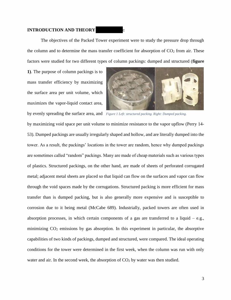
INTRODUCTION AND THEORY (Mikey Zhou):
The objectives of the Packed Tower experiment were to study the pressure drop through
the column and to determine the mass transfer coefficient for absorption of CO2 from air. These
factors were studied for two different types of column packings: dumped and structured (figure
1). The purpose of column packings is to
mass transfer efficiency by maximizing
the surface area per unit volume, which
maximizes the vapor-liquid contact area,
by evenly spreading the surface area, and
by maximizing void space per unit volume to minimize resistance to the vapor upflow (Perry 14-
53). Dumped packings are usually irregularly shaped and hollow, and are literally dumped into the
tower. As a result, the packings’ locations in the tower are random, hence why dumped packings
are sometimes called “random” packings. Many are made of cheap materials such as various types
of plastics. Structured packings, on the other hand, are made of sheets of perforated corrugated
metal; adjacent metal sheets are placed so that liquid can flow on the surfaces and vapor can flow
through the void spaces made by the corrugations. Structured packing is more efficient for mass
transfer than is dumped packing, but is also generally more expensive and is susceptible to
corrosion due to it being metal (McCabe 689). Industrially, packed towers are often used in
absorption processes, in which certain components of a gas are transferred to a liquid – e.g.,
minimizing CO2 emissions by gas absorption. In this experiment in particular, the absorptive
capabilities of two kinds of packings, dumped and structured, were compared. The ideal operating
conditions for the tower were determined in the first week, when the column was run with only
water and air. In the second week, the absorption of CO2 by water was then studied.
Figure 1 Left: structured packing. Right: Dumped packing.
4
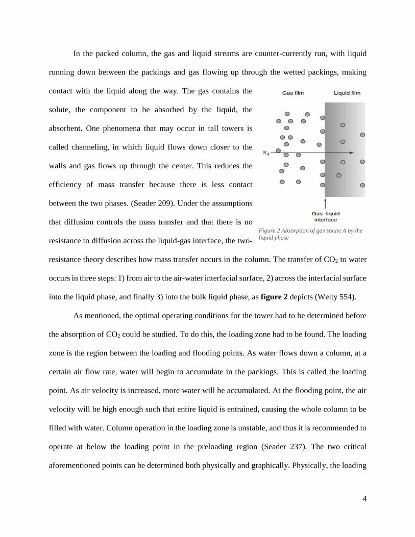
In the packed column, the gas and liquid streams are counter-currently run, with liquid
running down between the packings and gas flowing up through the wetted packings, making
contact with the liquid along the way. The gas contains the
solute, the component to be absorbed by the liquid, the
absorbent. One phenomena that may occur in tall towers is
called channeling, in which liquid flows down closer to the
walls and gas flows up through the center. This reduces the
efficiency of mass transfer because there is less contact
between the two phases. (Seader 209). Under the assumptions
that diffusion controls the mass transfer and that there is no
resistance to diffusion across the liquid-gas interface, the two-
resistance theory describes how mass transfer occurs in the column. The transfer of CO2 to water
occurs in three steps: 1) from air to the air-water interfacial surface, 2) across the interfacial surface
into the liquid phase, and finally 3) into the bulk liquid phase, as figure 2 depicts (Welty 554).
As mentioned, the optimal operating conditions for the tower had to be determined before
the absorption of CO2 could be studied. To do this, the loading zone had to be found. The loading
zone is the region between the loading and flooding points. As water flows down a column, at a
certain air flow rate, water will begin to accumulate in the packings. This is called the loading
point. As air velocity is increased, more water will be accumulated. At the flooding point, the air
velocity will be high enough such that entire liquid is entrained, causing the whole column to be
filled with water. Column operation in the loading zone is unstable, and thus it is recommended to
operate at below the loading point in the preloading region (Seader 237). The two critical
aforementioned points can be determined both physically and graphically. Physically, the loading
Figure 2 Absorption of gas solute A by the
liquid phase

5
point can be observed when surges of air can be seen moving up the column. The flooding point
can be seen when water has been pushed out of the top of the column by the air. Graphically, these
points can be determined from a log-log plot of the following equation, which expresses pressure
drop as a function of gas velocity (lab manual):
Δ𝑃 = 𝑎𝑉𝑔𝑏 (𝐸𝑞′𝑛 1)
where Δ𝑃 is the pressure drop per unit height of packing, 𝑎 and 𝑏 are constants, and 𝑉𝑔 is the
superficial gas velocity. In a log-log plot, 𝑎 would be the y-intercept and 𝑏 would be the slope.
During a dry run, the slope of the line on the plot should be approximately 1.8 (McCabe 691).
When there is water flowing in the system, the slope of the curve will initially also be 1.8. At the
loading point, as the air begins to slow the downflowing liquid causing increased water
accumulation, the pressure drop will rise suddenly due to there being less available space through
which gas can flow. This will increase the slope, thereby causing the curve to break from linearity.
An even more drastic rise in pressure drop, and thus slope, occurs at the flooding point. According
to McCabe, the operational gas velocity is sometimes chosen to be one half the flooding velocity
(McCabe 692).
With the optimal operating conditions determined, the absorption of CO2 by water can now
be studied. As stated previously, the two-resistance theory claims that mass transfer is controlled
by a concentration gradient. Equation 2 relates the overall mass transfer coefficient, 𝐾𝐿 , to the
individual phase coefficients:
1
𝐾𝐿=
1
𝑚𝑘𝐺+
1
𝑘𝐿 (𝐸𝑞′𝑛 2)
where 𝑘𝐺 and 𝑘𝐿 are the individual phase coefficients. However, because CO2 has a low solubility
in water, the system is said to be liquid-phase controlled and 𝐾𝐿 is essentially equal to 𝑘𝐿 (Welty
560). Correlated values of 𝐾𝐿 are found using equation 3 (Welty 587):
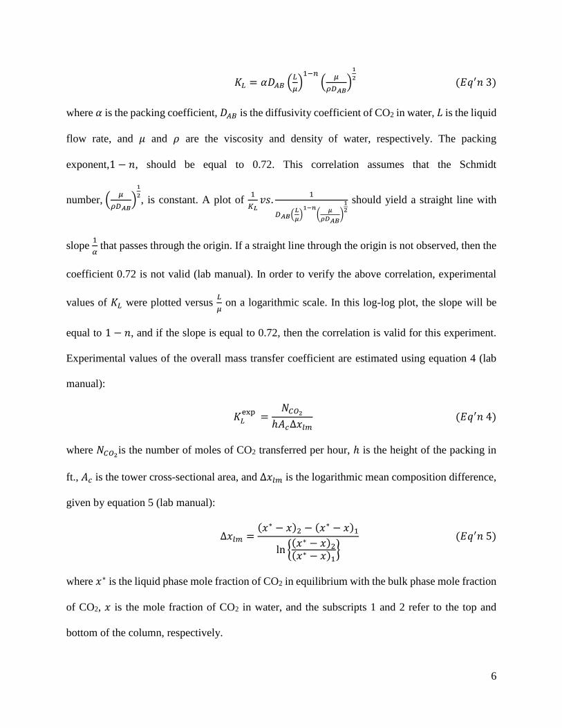
6
𝐾𝐿 = 𝛼𝐷𝐴𝐵 (𝐿
𝜇)1−𝑛
(𝜇
𝜌𝐷𝐴𝐵)
1
2 (𝐸𝑞′𝑛 3)
where 𝛼 is the packing coefficient, 𝐷𝐴𝐵 is the diffusivity coefficient of CO2 in water, 𝐿 is the liquid
flow rate, and 𝜇 and 𝜌 are the viscosity and density of water, respectively. The packing
exponent,1 − 𝑛, should be equal to 0.72. This correlation assumes that the Schmidt
number, (𝜇
𝜌𝐷𝐴𝐵)
1
2, is constant. A plot of
1
𝐾𝐿𝑣𝑠.
1
𝐷𝐴𝐵(𝐿
𝜇)1−𝑛
(𝜇
𝜌𝐷𝐴𝐵)
12
should yield a straight line with
slope 1
𝛼 that passes through the origin. If a straight line through the origin is not observed, then the
coefficient 0.72 is not valid (lab manual). In order to verify the above correlation, experimental
values of 𝐾𝐿 were plotted versus 𝐿
𝜇 on a logarithmic scale. In this log-log plot, the slope will be
equal to 1 − 𝑛, and if the slope is equal to 0.72, then the correlation is valid for this experiment.
Experimental values of the overall mass transfer coefficient are estimated using equation 4 (lab
manual):
𝐾𝐿exp
=𝑁𝐶𝑂2
ℎ𝐴𝑐Δ𝑥𝑙𝑚 (𝐸𝑞′𝑛 4)
where 𝑁𝐶𝑂2is the number of moles of CO2 transferred per hour, ℎ is the height of the packing in
ft., 𝐴𝑐 is the tower cross-sectional area, and Δ𝑥𝑙𝑚 is the logarithmic mean composition difference,
given by equation 5 (lab manual):
Δ𝑥𝑙𝑚 =(𝑥∗ − 𝑥)2 − (𝑥
∗ − 𝑥)1
ln {(𝑥∗ − 𝑥)2(𝑥∗ − 𝑥)1
} (𝐸𝑞′𝑛 5)
where 𝑥∗ is the liquid phase mole fraction of CO2 in equilibrium with the bulk phase mole fraction
of CO2, 𝑥 is the mole fraction of CO2 in water, and the subscripts 1 and 2 refer to the top and
bottom of the column, respectively.
7
APPARATUS AND PROCEDURES (Eddie Rich):
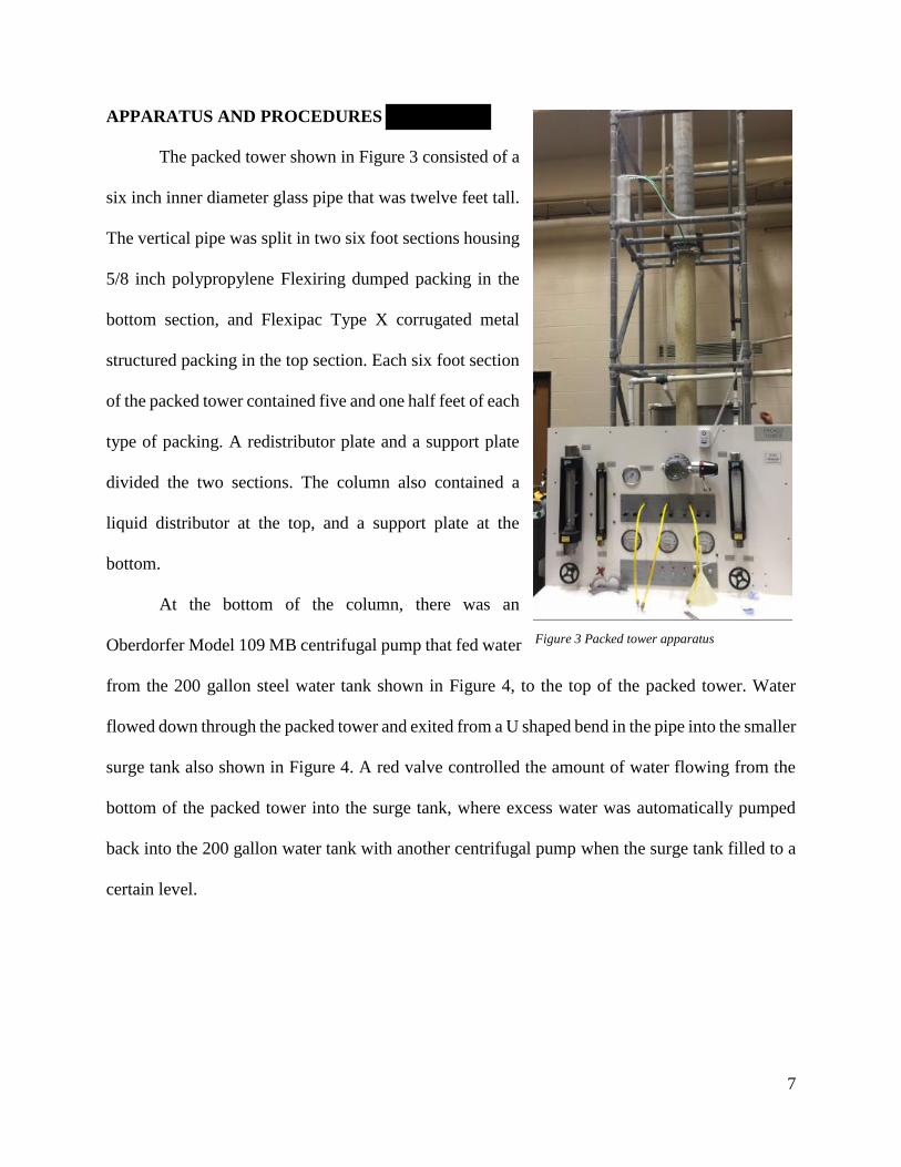
The packed tower shown in Figure 3 consisted of a
six inch inner diameter glass pipe that was twelve feet tall.
The vertical pipe was split in two six foot sections housing
5/8 inch polypropylene Flexiring dumped packing in the
bottom section, and Flexipac Type X corrugated metal
structured packing in the top section. Each six foot section
of the packed tower contained five and one half feet of each
type of packing. A redistributor plate and a support plate
divided the two sections. The column also contained a
liquid distributor at the top, and a support plate at the
bottom.
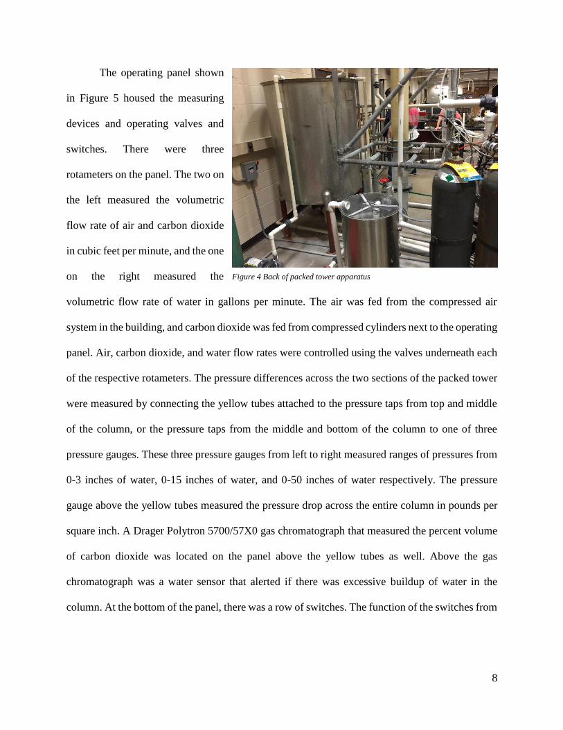
At the bottom of the column, there was an
Oberdorfer Model 109 MB centrifugal pump that fed water
from the 200 gallon steel water tank shown in Figure 4, to the top of the packed tower. Water
flowed down through the packed tower and exited from a U shaped bend in the pipe into the smaller
surge tank also shown in Figure 4. A red valve controlled the amount of water flowing from the
bottom of the packed tower into the surge tank, where excess water was automatically pumped
back into the 200 gallon water tank with another centrifugal pump when the surge tank filled to a
certain level.
Figure 3 Packed tower apparatus
8
The operating panel shown
in Figure 5 housed the measuring
devices and operating valves and
switches. There were three
rotameters on the panel. The two on
the left measured the volumetric
flow rate of air and carbon dioxide
in cubic feet per minute, and the one
on the right measured the
volumetric flow rate of water in gallons per minute. The air was fed from the compressed air
system in the building, and carbon dioxide was fed from compressed cylinders next to the operating
panel. Air, carbon dioxide, and water flow rates were controlled using the valves underneath each
of the respective rotameters. The pressure differences across the two sections of the packed tower
were measured by connecting the yellow tubes attached to the pressure taps from top and middle
of the column, or the pressure taps from the middle and bottom of the column to one of three
pressure gauges. These three pressure gauges from left to right measured ranges of pressures from
0-3 inches of water, 0-15 inches of water, and 0-50 inches of water respectively. The pressure
gauge above the yellow tubes measured the pressure drop across the entire column in pounds per
square inch. A Drager Polytron 5700/57X0 gas chromatograph that measured the percent volume
of carbon dioxide was located on the panel above the yellow tubes as well. Above the gas
chromatograph was a water sensor that alerted if there was excessive buildup of water in the
column. At the bottom of the panel, there was a row of switches. The function of the switches from
Figure 4 Back of packed tower apparatus

9
left to right were to turn on the recovery pump, zero the meters, turn on carbon dioxide heaters,
and turn on the feed pump and sample pump.
Initially for the first part of the experiment, the drain valve exiting from the 200 gallon
water tank was closed, and the tank was filled with water. The system was first operated with only
air running through the packed tower to find the pressure difference for the dry column. This was
accomplished by slowly increasing the air feed by an interval of 5 cubic feet per minute up to 45
cubic feet per minute by turning the air valve counter-clockwise. The pressure differences across
the top section, bottom section, and entire column were recorded for the various air flow rates used
during the dry run. As the pressure difference increased, the pressure gauges of higher ranges were
used. Once the pressure differences across the entire column, top section, and bottom section were
recorded for various air flow rates through the dry column, the feed and recovery pump switches
were turned on. The water control valve was then opened until the feed reached ten percent of the
Figure 5 Packed tower apparatus operating panel

10
pumps maximum flow rate of thirty gallons per minute. With water flowing through the system,
excess water will build up at the bottom of the column. The red valve in Figure 3 allows the excess
water to flow into the recovery tank. An ideal level that is marked on the tube at the bottom of the
column is maintained by opening or closing the red valve to control the buildup of water. Before
each pressure difference was measured, the meters were zeroed using the designated switch at the
bottom of the operating panel. Once the water flow rates increased to twenty percent and above,
loading and flooding was observed at higher air flow rates. Loading began when air can visually
be seen rising and pushing froth up the column. It can also be observed by a rapidly increasing
pressure difference across the top section, bottom section, and entire column. Flooding was
reached when the log-log plot of change in pressure to the gas velocity broke linearity. Care should
be taken when increasing the air flow rate to ensure excessive flooding doesn’t occur. After the
loading and flooding zones were identified for the different water and air flow rates, the system
was shut down. This was done by closing the water and air valves, turning off the feed pump,
opening the drain valve for the water tank, and purging the recovery tank.
During the second part of the experiment, the apparatus was operated in a similar way as
the first part of the experiment, except that the 200 gallon tank is filled with a 0.2 N water and soda
ash mixture, and carbon dioxide was fed into the system along with air. To start the process, the
water tank was filled with a soda ash and water mixture, the recovery pump and feed pump was
turned on, and the drain valve exiting the surge tank was closed. The water flow rate was then set
at 40% while the air flow rate was set at a constant 13 SCFM. The carbon dioxide heaters were
then turned on to keep the lines from freezing. A manifold regulator for carbon dioxide was then
set between 40 and 50 pounds per square inch, and carbon dioxide was introduced to the system.
The sample pump was then tuned on so that the volume percent of carbon dioxide could be
11
measured. The carbon dioxide flow rate was set at 0.4 SCFM to ensure that the percent volume of
carbon dioxide did not exceed the maximum measureable value of the gas chromatograph. Gas
chromatograph measurements were then recorded at the entrance, middle, and exit of the column,
after two minutes of the column reaching operating conditions. This was then repeated at constant
air and carbon dioxide flow rates, while taking pressure drop and carbon dioxide volume percent
data for different water flow rates ranging between 10-40%. After all of the data was obtained,
the system was shut down. This was accomplished by first completely closing the water flow rate
valve, and turning off the feed pump, sample pump, and carbon dioxide heaters. The air and carbon
dioxide control valves were then closed, followed by closing the carbon dioxide tank valves. The
column was then allowed to drain. The drain valves were then opened for the water and recovery
tanks.
Safety precautions were taken during the setup and operation of the packed tower unit, to
ensure no harm occurred during the laboratory. High voltage centrifugal pumps were utilized in
the experiment, so care was taken to avoid electric shock. Safety glasses were always worn
throughout the experiment. Soda ash is a skin and lung irritant, so the teacher assistant for the lab
wore the necessary safety equipment while making the soda ash and water mixture.
RESULTS AND DISCUSSION (Xiaorong Zhang):
The result of this experiment is separated into two parts according to two weeks of the
experiment. The first week’s experiment is to find the effective loading region of the packed
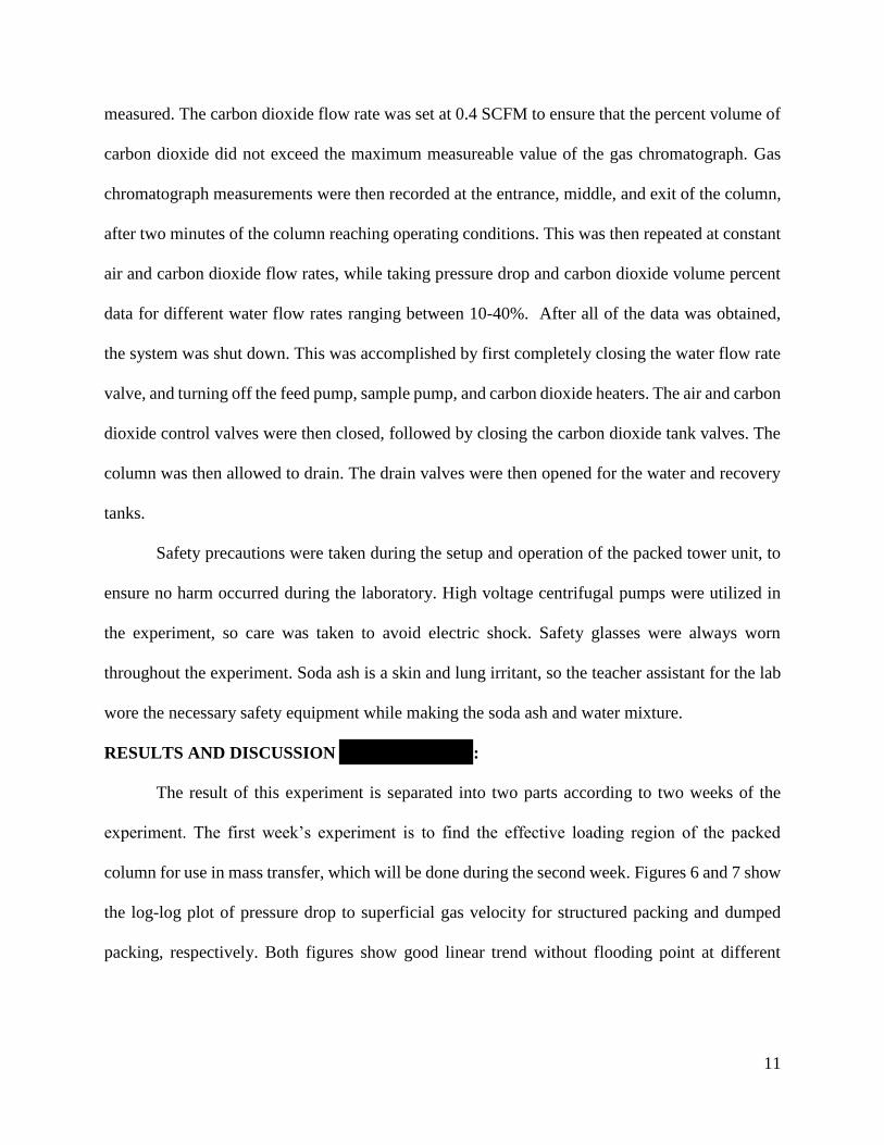
column for use in mass transfer, which will be done during the second week. Figures 6 and 7 show
the log-log plot of pressure drop to superficial gas velocity for structured packing and dumped
packing, respectively. Both figures show good linear trend without flooding point at different
12
percentages of max water flow rates. The flooding point is defined as the point which departs from
the linear trend in the figures. In addition, the loading point is defined as the point before the
flooding point. From both figures, flooding occurred at higher gas velocities for each run, and it
occurred at a relatively lower gas velocities as the percent max water flow rate increased.
Comparing the figures for structured and dumped packing, structured packing obtained a lower
pressure with different water flows, since the data points were more concentrated than in the
dumped packing from the figures.
13
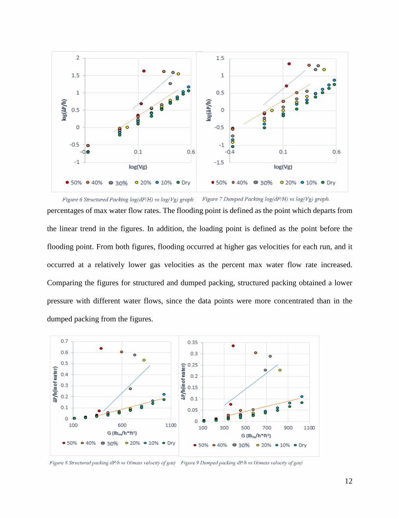
Figures 8 and 9 show the pressure drop versus gas mass velocity for structured and dumped
packing. The loading and flooding lines were indicated as orange and blue on the graph for both
structured and dumped packing. Since not enough data after loading was obtained, the flooding
line might not be accurate, however, the trend can be seen easily on the graph. The flooding
occurred at high gas mass velocity with low percent max water flow and at low gas mass velocity
with high percent max water flow. The pressure drop at the loading line is below 0.2 in inches of
water for structured packing, while for dumped packing it is below 0.1, each of which are varied
with different water flows and air flows. These values increase as water flow rate increases. A
change in the water flow rate causes a significant difference on the graph. It is safe to conclude
that water flow was the main factor to determine loading and flooding points. Comparing the two
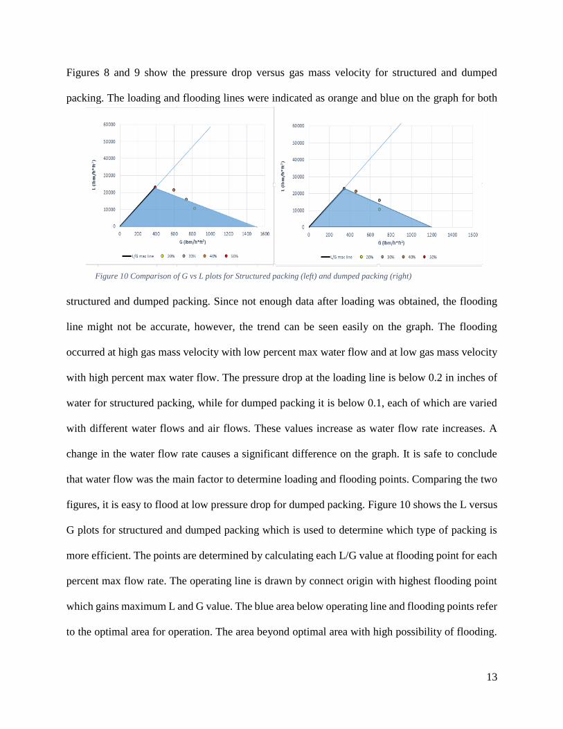
figures, it is easy to flood at low pressure drop for dumped packing. Figure 10 shows the L versus
G plots for structured and dumped packing which is used to determine which type of packing is
more efficient. The points are determined by calculating each L/G value at flooding point for each
percent max flow rate. The operating line is drawn by connect origin with highest flooding point
which gains maximum L and G value. The blue area below operating line and flooding points refer
to the optimal area for operation. The area beyond optimal area with high possibility of flooding.
Figure 10 Comparison of G vs L plots for Structured packing (left) and dumped packing (right)

14
The optimal area for structured packing obtains larger area due to its larger base. It can be inferred
from this graph that structured packing is more efficient than dumped packing. It also confirms the
conclusion we made previously.
.
y = 0.001756652xR² = 0.941100993
y = 0.001844930xR² = 0.922722441
0
0.001
0.002
0.003
0.004
0.005
0.006
0 0.5 1 1.5 2 2.5
1/K
La
1/(DAB(L/μ)0.72(Sc)0.5)
Structured
Dumped
y = 0.705x + 0.0193R² = 0.9599
y = 0.7645x - 0.2066R² = 0.9484
2.3
2.4
2.5
2.6
2.7
2.8
2.9
3.3 3.4 3.5 3.6 3.7 3.8 3.9 4
log(
KLa
)
log(L/μ)
log-log
Structured
Dumped
Figure 11 Sherwood and Holloway correlation for structured and dumped packing
Figure 12 log-log plot of KLa to L/μ for structured and dumped packing.
15
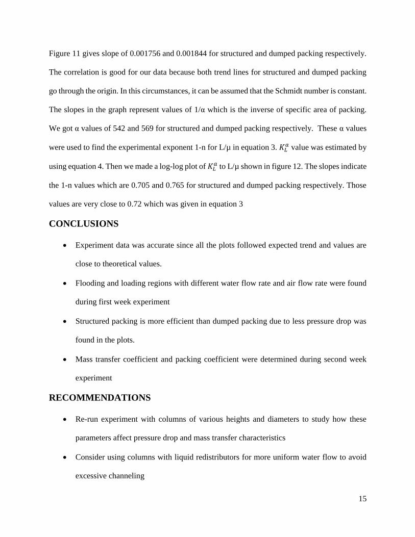
Figure 11 gives slope of 0.001756 and 0.001844 for structured and dumped packing respectively.
The correlation is good for our data because both trend lines for structured and dumped packing
go through the origin. In this circumstances, it can be assumed that the Schmidt number is constant.
The slopes in the graph represent values of 1/α which is the inverse of specific area of packing.
We got α values of 542 and 569 for structured and dumped packing respectively. These α values
were used to find the experimental exponent 1-n for L/µ in equation 3. 𝐾𝐿𝑎 value was estimated by
using equation 4. Then we made a log-log plot of 𝐾𝐿𝑎 to L/µ shown in figure 12. The slopes indicate
the 1-n values which are 0.705 and 0.765 for structured and dumped packing respectively. Those
values are very close to 0.72 which was given in equation 3
CONCLUSIONS
Experiment data was accurate since all the plots followed expected trend and values are
close to theoretical values.
Flooding and loading regions with different water flow rate and air flow rate were found
during first week experiment
Structured packing is more efficient than dumped packing due to less pressure drop was
found in the plots.
Mass transfer coefficient and packing coefficient were determined during second week
experiment
RECOMMENDATIONS
Re-run experiment with columns of various heights and diameters to study how these
parameters affect pressure drop and mass transfer characteristics
Consider using columns with liquid redistributors for more uniform water flow to avoid
excessive channeling

16
For more accurate determination of flooding velocity, increase water flow rate by smaller
intervals during the first week of experiment
REFERENCES
Lab Manual, Exp VI Packed Tower. (n.d.). Retrieved from learn.ou.edu
McCabe, W., Smith, J., & Harriott, P. (1993). Unit Operations of Chemical Engineering.
(5th ed.) McGraw-Hill Book Co.
Perry, Robert. (2008). Perry’s Chemical Engineers’ Handbook, (8th ed.) McGraw-Hill
Professional.
Seader, J. D., & Henley, E. J. (2005). Separation Process Principles. Chichester: John Wiley.
Welty, J., Wicks, C., Rorrer, G., & Wilson, R. (2008). Fundamentals of Momentum, Heat, and
Mass Transfer. (5th ed.) John Wiley and Sons, Inc.

17
APPENDIX (Eric Henderson):
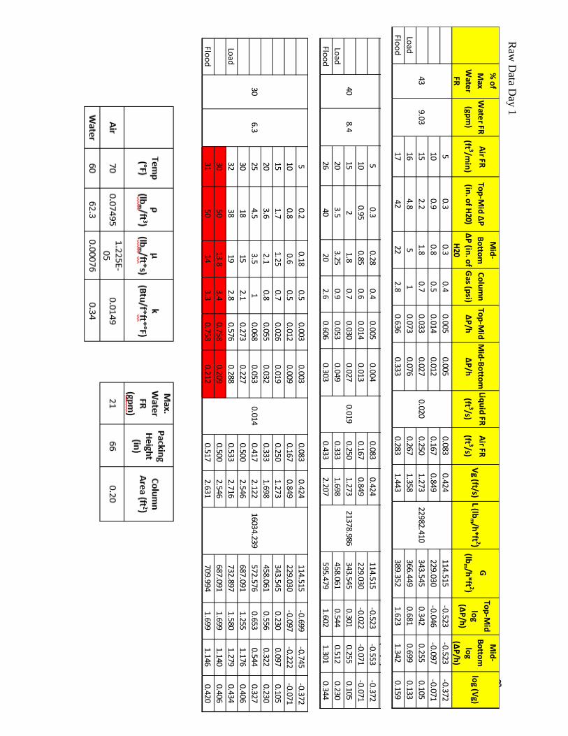
% Max water flow rate, Air FR, Top-Mid ΔP, Mid-Bottom ΔP, and Column Gas pressure are
measured experimentally. [Flow Rate: FR]
Calculations are carried out for 40% max water flow-rate:
Water FR = % 𝑀𝑎𝑥 𝑊𝑎𝑡𝑒𝑟 𝐹𝑅
𝑀𝑎𝑥 𝑊𝑎𝑡𝑒𝑟 𝐹𝑅∗ 100 =
40
21∗ 100 = 8.4 𝑔𝑝𝑚
Top-Mid ΔP/h = 𝑇𝑜𝑝−𝑀𝑖𝑑 ΔP
𝑃𝑎𝑐𝑘𝑖𝑛𝑔 ℎ𝑒𝑖𝑔ℎ𝑡=0.3 𝑖𝑛 𝐻2𝑂
5.5𝑓𝑡∗12𝑖𝑛
𝑓𝑡
=0.3 𝑖𝑛 𝐻2𝑂
66 𝑖𝑛= 0.005
Mid-Bottom ΔP/h = 0.28 𝑖𝑛 𝐻2𝑂
66 𝑖𝑛= 0.004
1 ft3 = 7.48 gal
Liquid FR = 𝑊𝑎𝑡𝑒𝑟 𝐹𝑅 [𝑔𝑝𝑚]
7.48 𝑔𝑎𝑙∗60𝑠
𝑚𝑖𝑛
=8.4 𝑔𝑝𝑚
7.48 𝑔𝑎𝑙∗60𝑠
𝑚𝑖𝑛
= 0.019𝑓𝑡3
𝑠
Cross-Sectional Area = 𝜋∗0.52
4 = 0.196 𝑓𝑡2 where 0.5 ft is the column diameter
Air FR = 𝐸𝑥𝑝𝑒𝑟𝑖𝑚𝑒𝑛𝑡𝑎𝑙 𝐴𝑖𝑟 𝐹𝑅
𝑈𝑛𝑖𝑡 𝐶𝑜𝑛𝑣𝑒𝑟𝑠𝑖𝑜𝑛=
5𝑓𝑡3
𝑚𝑖𝑛
60𝑠
𝑚𝑖𝑛
= 0.083𝑓𝑡3
𝑠
Air velocity = Vg = 𝐴𝑖𝑟 𝐹𝑅
𝐶𝑜𝑙𝑢𝑚𝑛 𝐴𝑟𝑒𝑎=0.083
𝑓𝑡3
𝑠
0.20 𝑓𝑡2= 0.424
𝑓𝑡
𝑠
Liquid Molar FR = L = 𝐷𝑒𝑛𝑠𝑖𝑡𝑦 𝑜𝑓 𝑊𝑎𝑡𝑒𝑟∗𝐿𝑖𝑞𝑢𝑖𝑑 𝐹𝑅
𝐶𝑜𝑙𝑢𝑚𝑛 𝐴𝑟𝑒𝑎=62.3
𝑙𝑏𝑚𝑓𝑡3
∗0.019𝑓𝑡3
𝑠
0.20 𝑓𝑡2∗ 3600
𝑠
ℎ𝑟= 21378.99
𝑙𝑏𝑚
ℎ∗𝑓𝑡2
Air Molar FR = G = 𝐷𝑒𝑛𝑠𝑖𝑡𝑦 𝑜𝑓 𝐴𝑖𝑟∗𝐴𝑖𝑟 𝐹𝑅
𝐶𝑜𝑙𝑢𝑚𝑛 𝐴𝑟𝑒𝑎=0.075
𝑙𝑏𝑚𝑓𝑡3
∗0.083𝑓𝑡3
𝑠
0.20 𝑓𝑡2∗ 3600
𝑠
ℎ𝑟= 114.52
𝑙𝑏𝑚
ℎ∗𝑓𝑡2
Top-Mid log (ΔP/h) = log10 (Top-Mid ΔP) = log10 (0.3) = -0.523
Mid-Bottom log ΔP/h = log10 (Mid-Bottom ΔP) = log10 (0.28) = -0.553
log10 (Air Velocity) = log10 (Vg) = log10 (0.424) = -0.372
18
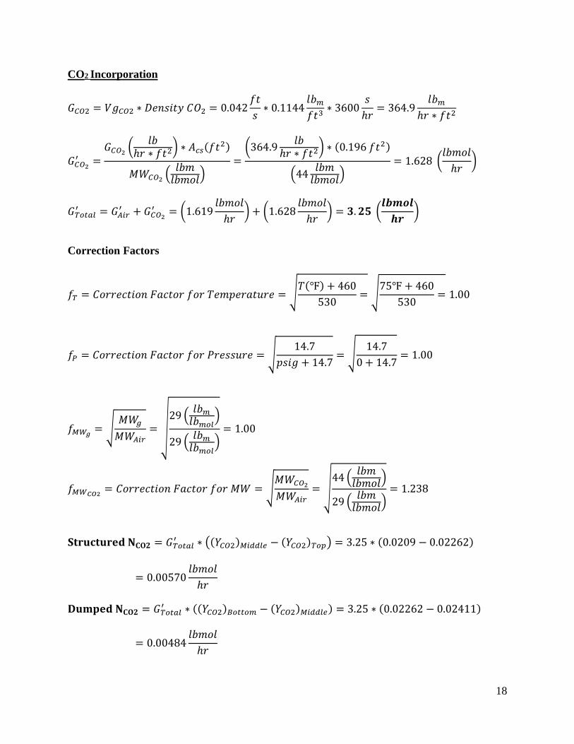
CO2 Incorporation
𝐺𝐶𝑂2 = 𝑉𝑔𝐶𝑂2 ∗ 𝐷𝑒𝑛𝑠𝑖𝑡𝑦 𝐶𝑂2 = 0.042𝑓𝑡
𝑠∗ 0.1144
𝑙𝑏𝑚𝑓𝑡3
∗ 3600𝑠
ℎ𝑟= 364.9
𝑙𝑏𝑚ℎ𝑟 ∗ 𝑓𝑡2
𝐺𝐶𝑂2′ =
𝐺𝐶𝑂2 (𝑙𝑏
ℎ𝑟 ∗ 𝑓𝑡2) ∗ 𝐴𝑐𝑠(𝑓𝑡
2)
𝑀𝑊𝐶𝑂2 (𝑙𝑏𝑚𝑙𝑏𝑚𝑜𝑙
)=(364.9
𝑙𝑏ℎ𝑟 ∗ 𝑓𝑡2
) ∗ (0.196 𝑓𝑡2)
(44𝑙𝑏𝑚𝑙𝑏𝑚𝑜𝑙
)= 1.628 (
𝑙𝑏𝑚𝑜𝑙
ℎ𝑟)
𝐺𝑇𝑜𝑡𝑎𝑙′ = 𝐺𝐴𝑖𝑟
′ + 𝐺𝐶𝑂2′ = (1.619
𝑙𝑏𝑚𝑜𝑙
ℎ𝑟) + (1.628
𝑙𝑏𝑚𝑜𝑙
ℎ𝑟) = 𝟑. 𝟐𝟓 (
𝒍𝒃𝒎𝒐𝒍
𝒉𝒓)
Correction Factors
𝑓𝑇 = 𝐶𝑜𝑟𝑟𝑒𝑐𝑡𝑖𝑜𝑛 𝐹𝑎𝑐𝑡𝑜𝑟 𝑓𝑜𝑟 𝑇𝑒𝑚𝑝𝑒𝑟𝑎𝑡𝑢𝑟𝑒 = √𝑇(℉) + 460
530= √
75℉ + 460
530= 1.00
𝑓𝑃 = 𝐶𝑜𝑟𝑟𝑒𝑐𝑡𝑖𝑜𝑛 𝐹𝑎𝑐𝑡𝑜𝑟 𝑓𝑜𝑟 𝑃𝑟𝑒𝑠𝑠𝑢𝑟𝑒 = √14.7
𝑝𝑠𝑖𝑔 + 14.7= √
14.7
0 + 14.7= 1.00
𝑓𝑀𝑊𝑔 = √𝑀𝑊𝑔
𝑀𝑊𝐴𝑖𝑟= √
29 (𝑙𝑏𝑚𝑙𝑏𝑚𝑜𝑙
)
29 (𝑙𝑏𝑚𝑙𝑏𝑚𝑜𝑙
)= 1.00
𝑓𝑀𝑊𝐶𝑂2= 𝐶𝑜𝑟𝑟𝑒𝑐𝑡𝑖𝑜𝑛 𝐹𝑎𝑐𝑡𝑜𝑟 𝑓𝑜𝑟 𝑀𝑊 = √
𝑀𝑊𝐶𝑂2𝑀𝑊𝐴𝑖𝑟
= √44 (
𝑙𝑏𝑚𝑙𝑏𝑚𝑜𝑙
)
29 (𝑙𝑏𝑚𝑙𝑏𝑚𝑜𝑙
)= 1.238
𝐒𝐭𝐫𝐮𝐜𝐭𝐮𝐫𝐞𝐝 𝐍𝐂𝐎𝟐 = 𝐺𝑇𝑜𝑡𝑎𝑙′ ∗ ((𝑌𝐶𝑂2)𝑀𝑖𝑑𝑑𝑙𝑒 − (𝑌𝐶𝑂2)𝑇𝑜𝑝) = 3.25 ∗ (0.0209 − 0.02262)
= 0.00570𝑙𝑏𝑚𝑜𝑙
ℎ𝑟
𝐃𝐮𝐦𝐩𝐞𝐝 𝐍𝐂𝐎𝟐 = 𝐺𝑇𝑜𝑡𝑎𝑙′ ∗ ((𝑌𝐶𝑂2)𝐵𝑜𝑡𝑡𝑜𝑚 − (𝑌𝐶𝑂2)𝑀𝑖𝑑𝑑𝑙𝑒) = 3.25 ∗ (0.02262 − 0.02411)
= 0.00484𝑙𝑏𝑚𝑜𝑙
ℎ𝑟

19
𝑺𝒕𝒓𝒖𝒄𝒕𝒖𝒓𝒆𝒅 𝜟𝑿𝒍𝒎 =(𝑥∗ − 𝑥)𝑡𝑜𝑝 − (𝑥
∗ − 𝑥)𝑚𝑖𝑑𝑑𝑙𝑒
ln {(𝑥∗ − 𝑥)𝑡𝑜𝑝(𝑥∗ − 𝑥)𝑚𝑖𝑑𝑑𝑙𝑒
}
=(1.93 ∗ 10−5 − 0) − (2.1 ∗ 10−5 − 0)
ln (1.93 ∗ 10−5 − 02.1 ∗ 10−5 − 0
)
= 𝟐. 𝟎𝟏𝟏 ∗ 𝟏𝟎−𝟓
𝑫𝒖𝒎𝒑𝒆𝒅 𝜟𝑿𝒍𝒎 =(𝑥∗ − 𝑥)𝑀𝑖𝑑𝑑𝑙𝑒 − (𝑥
∗ − 𝑥) 𝐵𝑜𝑡𝑜𝑚
ln {(𝑥∗ − 𝑥)𝑀𝑖𝑑𝑑𝑙𝑒(𝑥∗ − 𝑥)𝐵𝑜𝑡𝑡𝑜𝑚
}=(2.1 − 0) − (2.237 ∗ 10−5 − 0)
ln (2.1 ∗ 10−5 − 02.237 ∗ 10−5 − 0
)
= 𝟐. 𝟏𝟔𝟔 ∗ 𝟏𝟎−𝟓
𝟏/𝑲𝑳𝒂 =1
𝑁 (𝑙𝑏𝑚𝑜𝑙ℎ𝑟
)
∆𝑋𝑙𝑚 ∗ ℎ(𝑓𝑡) ∗ 𝐴𝑐𝑠(𝑓𝑡2)
=1
(0.0057)𝑙𝑏𝑚𝑜𝑙ℎ𝑟
(4.83 ∗ 10−5) ∗ (5.5𝑓𝑡) ∗ (0.196𝑓𝑡2)
= 0.0038 (𝑙𝑏𝑚𝑜𝑙
ℎ𝑟 ∗ 𝑓𝑡2)−1
1
𝐷𝐴𝐵 (𝑓𝑡2
ℎ𝑟) ∗ (
𝐿 (𝑙𝑏𝑚
ℎ𝑟 ∗ 𝑓𝑡2)
𝜇 (𝑙𝑏
ℎ𝑟 ∗ 𝑓𝑡))
0.72
∗
(
𝜇 (
𝑙𝑏ℎ𝑟 ∗ 𝑓𝑡
)
𝜌 (𝑙𝑏𝑚𝑓𝑡3
)∗ 𝐷𝐴𝐵 (
𝑓𝑡2
ℎ𝑟)
)
0.5
=1
(6.855 ∗ 10−5𝑓𝑡2
ℎ𝑟) ∗ (
(5497.09𝑙𝑏𝑚
ℎ𝑟 ∗ 𝑓𝑡2)
(0.000669 ∗ 3600𝑙𝑏
ℎ𝑟 ∗ 𝑓𝑡))
0.72
∗
(
(0.000669 ∗ 3600
𝑙𝑏ℎ𝑟 ∗ 𝑓𝑡
)
(62.261𝑙𝑏𝑚𝑓𝑡3
)∗ (6.855 ∗ 10−5
𝑓𝑡2
ℎ𝑟)
)
0.5
= 2.3453
o 𝐷𝐴𝐵 = 𝐷𝑖𝑓𝑓𝑢𝑠𝑖𝑣𝑖𝑡𝑦 𝑜𝑓 𝐶𝑎𝑟𝑏𝑜𝑛 𝐷𝑖𝑜𝑥𝑖𝑑𝑒 𝑖𝑛 𝑊𝑎𝑡𝑒𝑟
o 𝜇 = 𝑉𝑖𝑠𝑐𝑜𝑠𝑖𝑡𝑦 𝑜𝑓 𝑊𝑎𝑡𝑒𝑟

20
Supplementary Equations:
Middle of Tower:
L
GyGyLxxGyLxGyLx outinin
outoutoutinin
xin=0 because no CO2 enters with liquid phase
Equation becomes
G
L
yyx outin
out
o xout = Middle mole fraction of CO2 in liquid phase
o yin = Middle mole fraction of CO2 in vapor phase
o yout = Top mole fraction of CO2 in vapor phase
Bottom of Tower:
G
L
yyG
Lx
xinoutin
out
*
o xin = Middle mole fraction of CO2 in liquid phase
o xout = Bottom mole fraction of CO2 in liquid phase
o yin = Bottom mole fraction of CO2 in vapor phase
o yout = Middle mole fraction of CO2 in vapor phase
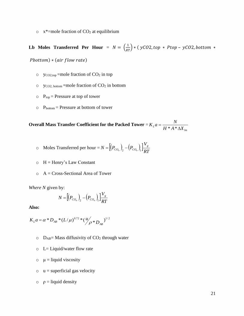
Mole Fraction of CO2 at equilibrium = x*= PCO2/HCO2
o H=Henry’s Law Constant (inches of H2O)
o P=Partial Pressure of CO2
21
o x*=mole fraction of CO2 at equilibrium
Lb Moles Transferred Per Hour = 𝑁 = (1
𝑅𝑇) ∗ ( 𝑦𝐶𝑂2, 𝑡𝑜𝑝 ∗ 𝑃𝑡𝑜𝑝 – 𝑦𝐶𝑂2, 𝑏𝑜𝑡𝑡𝑜𝑚 ∗
𝑃𝑏𝑜𝑡𝑡𝑜𝑚) ∗ (𝑎𝑖𝑟 𝑓𝑙𝑜𝑤 𝑟𝑎𝑡𝑒)
o yCO2,top =mole fraction of CO2 in top
o yCO2, bottom =mole fraction of CO2 in bottom
o Ptop = Pressure at top of tower
o Pbottom = Pressure at bottom of tower
Overall Mass Transfer Coefficient for the Packed Tower =lm
LXAH
NaK
**
o Moles Transferred per hour = RT
VPPN
g
COCO ww 12
o H = Henry’s Law Constant
o A = Cross-Sectional Area of Tower
Where N given by:
RT
VPPN
g
COCO ww 12
Also:
2/172.0 )*
(*)/(**AB
ABL DuLDaK
o DAB= Mass diffusivity of CO2 through water
o L= Liquid/water flow rate
o μ = liquid viscosity
o u = superficial gas velocity
o ρ = liquid density
22
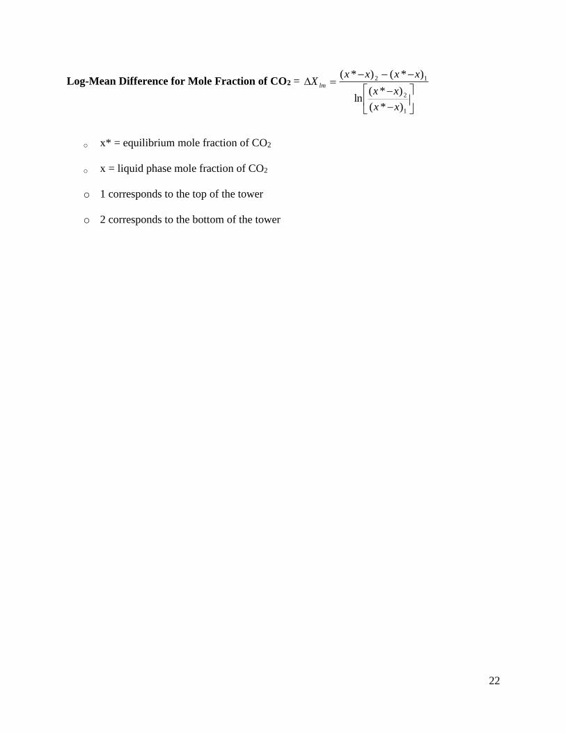
Log-Mean Difference for Mole Fraction of CO2 =
1
2
12
)*(
)*(ln
)*()*(
xx
xx
xxxxX lm
o x* = equilibrium mole fraction of CO2
o x = liquid phase mole fraction of CO2
o 1 corresponds to the top of the tower
o 2 corresponds to the bottom of the tower
23
% o
f
Max
Wate
r
FR
Wate
r FR
(gpm
)
Air FR
(ft3/m
in)
Top
-Mid
ΔP
(in. o
f H20)
Mid
-
Bo
ttom
ΔP
(in. o
f
H20
Co
lum
n
Gas (p
si)
Top
-Mid
ΔP
/h
Mid
-Bo
ttom
ΔP
/h
Liqu
id FR
(ft3/s)
Air FR
(ft3/s)
Vg (ft/s)
L (lbm
/h*ft
2)G
(lbm
/h*ft
2)
Top
-Mid
log
(ΔP
/h)
Mid
-
Bo
ttom
log
(ΔP
/h)
log (V
g)
50.3
0.30.4
0.0050.005
0.0830.424
114.515-0.523
-0.523-0.372
100.9
0.80.5
0.0140.012
0.1670.849
229.030-0.046
-0.097-0.071
152.2
1.80.7
0.0330.027
0.2501.273
343.5450.342
0.2550.105
Load
164.8
51
0.0730.076
0.2671.358
366.4490.681
0.6990.133
Floo
d17
4222
2.80.636
0.3330.283
1.443389.352
1.6231.342
0.159
439.03
0.02022982.410
% o
f
Max
Wate
r
FR
Wate
r FR
(gpm
)
Air FR
(ft 3/min
)
Top
-Mid
ΔP
(in. o
f H20)
Mid
-
Bo
ttom
ΔP
(in. o
f
H20
Co
lum
n
Gas (p
si)
Top
-Mid
ΔP
/h
Mid
-Bo
ttom
ΔP
/h
Liqu
id FR
(ft 3/s)
Air FR
(ft 3/s)V
g (ft/s)L (lb
m/h
*ft2)
G
(lbm
/h*ft
2)
Top
-Mid
log
(ΔP
/h)
Mid
-
Bo
ttom
log
(ΔP
/h)
log (V
g)
50.3
0.280.4
0.0050.004
0.0830.424
114.515-0.523
-0.553-0.372
100.95
0.850.6
0.0140.013
0.1670.849
229.030-0.022
-0.071-0.071
152
1.80.7
0.0300.027
0.2501.273
343.5450.301
0.2550.105
Load
203.5
3.250.9
0.0530.049
0.3331.698
458.0610.544
0.5120.230
Floo
d26
4020
2.60.606
0.3030.433
2.207595.479
1.6021.301
0.344
408.4
0.01921378.986
50.2
0.180.5
0.0030.003
0.0830.424
114.515-0.699
-0.745-0.372
100.8
0.60.5
0.0120.009
0.1670.849
229.030-0.097
-0.222-0.071
151.7
1.250.7
0.0260.019
0.2501.273
343.5450.230
0.0970.105
203.6
2.10.8
0.0550.032
0.3331.698
458.0610.556
0.3220.230
254.5
3.51
0.0680.053
0.4172.122
572.5760.653
0.5440.327
3018
152.1
0.2730.227
0.5002.546
687.0911.255
1.1760.406
Load
3238
192.8
0.5760.288
0.5332.716
732.8971.580
1.2790.434
3050
13.83.4
0.7580.209
0.5002.546
687.0911.699
1.1400.406
Floo
d31
5014
3.30.758
0.2120.517
2.631709.994
1.6991.146
0.420
306.3
0.01416034.239
Raw
Data D
ay 1
24
% o
f
Max
Wate
r
FR
Wate
r FR
(gpm
)
Air FR
(ft3/m
in)
Top
-Mid
ΔP
(in. o
f H20)
Mid
-
Bo
ttom
ΔP
(in. o
f
H20
Co
lum
n
Gas (p
si)
Top
-Mid
ΔP
/h
Mid
-Bo
ttom
ΔP
/h
Liqu
id FR
(ft3/s)
Air FR
(ft3/s)
Vg (ft/s)
L (lbm
/h*ft
2)G
(lbm
/h*ft
2)
Top
-Mid
log
(ΔP
/h)
Mid
-
Bo
ttom
log
(ΔP
/h)
log (V
g)
50.2
0.120.4
0.0030.002
0.0830.424
114.515-0.699
-0.921-0.372
100.72
0.50.5
0.0110.008
0.1670.849
229.030-0.143
-0.301-0.071
151.5
10.5
0.0230.015
0.2501.273
343.5450.176
0.0000.105
202.6
1.680.7
0.0390.025
0.3331.698
458.0610.415
0.2250.230
254
2.51
0.0610.038
0.4172.122
572.5760.602
0.3980.327
306
31.2
0.0910.045
0.5002.546
687.0910.778
0.4770.406
Floo
d35
215.8
1.50.318
0.0880.583
2.971801.606
1.3220.763
0.473
3635
152.75
0.5300.227
0.6003.056
824.5091.544
1.1760.485
204.2
0.00910689.493
50.2
0.140.45
0.0030.002
0.0830.424
114.515-0.699
-0.854-0.372
100.7
0.40.5
0.0110.006
0.1670.849
229.030-0.155
-0.398-0.071
151.5
0.80.5
0.0230.012
0.2501.273
343.5450.176
-0.0970.105
202.5
1.50.75
0.0380.023
0.3331.698
458.0610.398
0.1760.230
253.5
20.9
0.0530.030
0.4172.122
572.5760.544
0.3010.327
305.3
31.1
0.0800.045
0.5002.546
687.0910.724
0.4770.406
357.5
41.4
0.1140.061
0.5832.971
801.6060.875
0.6020.473
4010.6
5.41.75
0.1610.082
0.6673.395
916.1211.025
0.7320.531
4514.4
7.32.1
0.2180.111
0.7503.820
1030.6361.158
0.8630.582
102.1
0.0055344.746
50.19
0.090.4
0.0030.001
0.0830.424
114.515-0.721
-1.046-0.372
100.6
0.310.45
0.0090.005
0.1670.849
229.030-0.222
-0.509-0.071
151.25
0.690.5
0.0190.010
0.2501.273
343.5450.097
-0.1610.105
202.1
1.10.6
0.0320.017
0.3331.698
458.0610.322
0.0410.230
253.3
1.670.75
0.0500.025
0.4172.122
572.5760.519
0.2230.327
304.9
2.41
0.0740.036
0.5002.546
687.0910.690
0.3800.406
356.5
3.21.4
0.0980.048
0.5832.971
801.6060.813
0.5050.473
409
4.31.6
0.1360.065
0.6673.395
916.1210.954
0.6330.531
4511.5
5.52
0.1740.083
0.7503.820
1030.6361.061
0.7400.582
00
0.0000.000
25
Raw Data Day 2
Air Properties Water Properties CO2 Properties mo heat Column Specs
density 0.074887 lbm/ft^3 density 62.3 lbm/ft^3 density 0.1145 lbm/ft^3 Diameter 0.5 ft
viscosity viscosity viscosity 9.83E-06 lbm/fts Top h 5.5 ft
MW MW 18.016 MW 44.01 bottom h 5.5 ft
T 70 F T 70 F T
Packed TowerAir Flowrate
[SCFM]
Air
Flowrate
[ft3/s]
CO2
flowrate
[SCFM]
CO2
flowrate
[ft3/s]
GCO2
[lbm/h*ft2]
Gair
[lbm/h*ft2]VgCO2 [ft/s] Vgair [ft/s]
0.008250.173974Day 2 13 0.4 0.88604030.042034364.9068 238.87043
% of Max
Water FR
QWater
[gpm]QWater [ft
3/s]
Top-Mid
ΔP
[in H2O]
Mid-
Bottom ΔP
[in H2O]
Column P
[psi]
Top CO2
Vol%
Middle CO2
Vol%
Bottom CO2
Vol%
10 2.16 0.004813 1.2 0.5 0.4 3.12 3.38 3.6
15 3.24 0.007219 1.4 1.5 0.5 3.04 3.32 3.72
20 4.32 0.009625 1.5 2.1 0.5 2.92 3.28 3.68
25 5.4 0.012031 2.9 4 0.6 2.78 3.22 3.7
30 6.48 0.014438 3.6 4.8 0.75 2.64 3.12 3.7
35 7.56 0.016844 4.3 5.7 0.85 2.54 3.08 3.68
40 8.64 0.01925 4.5 7 0.9 2.52 3.04 3.72
P_top [atm]P_mid
[atm]
P_bottom
[atm]
CO2 Molarity
Tpo(mol/ft3)
CO2
Molarity
middle
CO2
Molarity
Bottom
air Molarity
Top
(mol/ft3)
air Molarity
middle
air Molarity
Bottom
1 1.002947 1.004175 0.0369882 0.040071 0.042679 1.7359015 1.731243 1.727301
1 1.003438 1.007122 0.0360398 0.039359 0.044101 1.7373349 1.732318 1.725151
1 1.003684 1.008841 0.0346172 0.038885 0.043627 1.7394851 1.733035 1.725867
1 1.007122 1.016945 0.0329574 0.038174 0.043864 1.7419936 1.73411 1.725509
1 1.008841 1.020629 0.0312977 0.036988 0.043864 1.7445021 1.735901 1.725509
1 1.01056 1.024558 0.0301122 0.036514 0.043627 1.7462939 1.736618 1.725867
1 1.011051 1.028241 0.0298751 0.03604 0.044101 1.7466523 1.737335 1.725151
26
Y CO2 Top Y CO2
middle
Y CO2
Bottom x_top x_mid x_bottom
0.020863 0.022622 0.024113 1.93E-05 2.1E-05 2.23745E-05
0.020323 0.022216 0.024927 1.88E-05 2.06E-05 2.31977E-05
0.019512 0.021945 0.024655 1.8E-05 2.04E-05 2.29843E-05
0.018568 0.021539 0.024791 1.72E-05 2E-05 2.32964E-05
0.017625 0.020863 0.024791 1.63E-05 1.94E-05 2.33808E-05
0.016951 0.020593 0.024655 1.57E-05 1.92E-05 2.33423E-05
0.016817 0.020323 0.024927 1.55E-05 1.9E-05 2.36841E-05
G'CO2
[lbm/hr]
G'air
[lbm/hr]
G'total
[lbm/hr]
structured
NCO2
[lbmol/hr]
Dumped
NCO2
[lbmol/hr]
structured
NCO3
[g/mol]
Dumped
NCO3
[g/mol]
0.00571221 0.00484135 2.591 2.195989
0.00614866 0.00880427 2.788971 3.993529
0.0079011 0.00880186 3.583859 3.992435
0.0096503 0.01056079 4.377279 4.790267
0.01051897 0.01275659 4.771299 5.78626
0.01182818 0.01319376 5.365145 5.984557
0.01138777 0.01495293 5.165377 6.7825
1.619548 3.247941.628393
structured
Δxlm
dumped
Δxlm
structured
1/KLa
dumped
1/KLaSc
L
[lbm/h*ft2]1/(DAB(L/μ)0.72(Sc)0.5) log(L/μ)
structured
Log(Kla)
dumped
log(Kla)
2.011E-05 2.166E-05 0.003802 0.004832 563.6308 5497.09 2.345339603 3.358404 2.419989 2.315867
1.968E-05 2.187E-05 0.003456 0.002683 563.6308 8245.635 1.751539882 3.534495 2.461465 2.571397
1.917E-05 2.164E-05 0.00262 0.002655 563.6308 10994.18 1.423849674 3.659434 2.581705 2.575881
1.856E-05 2.163E-05 0.002077 0.002212 563.6308 13742.72 1.212520056 3.756344 2.68247 2.655244
1.782E-05 2.135E-05 0.00183 0.001808 563.6308 16491.27 1.063355382 3.835525 2.737649 2.742847
1.739E-05 2.122E-05 0.001587 0.001737 563.6308 19239.81 0.95164889 3.902472 2.799324 2.760234
1.721E-05 2.125E-05 0.001632 0.001535 563.6308 21988.36 0.864415495 3.960464 2.787373 2.813994
F1 F2 F3 Corr.
Air 1 0.802955 1 0.802955
Water 1 1 1 1
CO2 1.238 1 1 1.238
CO2 Vg
(ft/s) air Vg (ft/s)
CO2 G
[lbm/h*ft2
]
air G
[lbm/h*ft2]
0.0420339 0.8860403 17.402 0.000
27
100% QWater
[gpm] QAir [pisg] Tower Across [ft
2]HCO2 [atm]
@ 70FDAB (cm2/s)
ρwater
(lbm/ft3)
ρair
(lbm/ft3)
ρCO2
(lbm/ft3)
Packing
Height [ft]
μwater
(lbm/ft-s)
21.6 8.1 0.196349541 1082.18 1.77E-05 62.3 0.074887 0.1144 5.5 0.000669
DAB (ft2/hr)
6.86E-05 0.66248
0.115
MW air (g/mol) 28.96
MW CO2 (g/mol) 44
0.00076
ρsoda ash (lbm/ft3)1
529.67
0.7302413
P atm
Air Temp (Rankine)
R (ft3*atm/R*lb-mol)


![[Ralph F. Strigle] Packed Tower Design and Applica(Bookos.org)](https://static.fdocuments.us/doc/165x107/54549a3cb1af9f9c328b4c20/ralph-f-strigle-packed-tower-design-and-applicabookosorg.jpg)