
GAME THEORETICAL FRAMEWORK FOR DISTRIBUTED DYNAMIC …
111
GAME THEORETICAL FRAMEWORK FOR DISTRIBUTED DYNAMIC CONTROL IN SMART GRIDS A Dissertation Presented to the Faculty of the Electrical and Computer Engineering Department University of Houston in Partial Fulfillment of the Requirements for the Degree Doctor of Philosophy in Electrical Engineering by Najmeh Forouzandehmehr December 2013
Transcript of GAME THEORETICAL FRAMEWORK FOR DISTRIBUTED DYNAMIC …
GAME THEORETICAL FRAMEWORK FOR DISTRIBUTED
DYNAMIC CONTROL IN SMART GRIDS
A DissertationPresented to
the Faculty of the Electrical and Computer Engineering Department
University of Houston
in Partial Fulfillmentof the Requirements for the Degree
Doctor of Philosophy
in Electrical Engineering
by
Najmeh Forouzandehmehr
December 2013

c⃝ Copyright by Najmeh Forouzandehmehr 2013
All Rights Reserved
GAME THEORETICAL FRAMEWORK FOR DISTRIBUTEDDYNAMIC CONTROL IN SMART GRIDS
Najmeh Forouzandehmehr
Approved:Chair of the CommitteeDr. Zhu Han, Associate ProfessorElectrical and Computer Engineering
Committee Members:Dr. Haluk Ogmen, ProfessorElectrical and Computer Engineering
Dr. Hamed Mohsenian-Rad, Assistant ProfessorElectrical and Computer EngineeringUniversity of California at Riverside, CA
Dr. Amin Khodaei, Assistant ProfessorElectrical and Computer EngineeringUniversity of Denver, CO
Dr. Wei-Chuan Shih, Assistant ProfessorElectrical and Computer Engineering
Dr. Suresh K. Khator, Associate Dean, Dr. Badrinath Roysam, Professor and Chairman,Cullen College of Engineering Electrical and Computer Engineering

Acknowledgements
The work presented in this dissertation would not have been possible without a num-
ber of people who have guided and supported me throughout the research process and
provided assistance for my venture.
I would like to express my deepest gratitude to my advisor, Dr. Zhu Han, for his
excellent guidance, caring, patience, and providing me with an excellent atmosphere for
doing research. He patiently provided the vision and encouragement necessary for me to
proceed through the doctoral program and complete my dissertation. His profound knowl-
edge and scientific curiosity have set high standards and are a constant source of inspiration
and his advice, both scholarly and non-academic, leave me greatly indebted. I would like
to thank Dr. Rong Zheng, Dr. Hamed Mohsenian-rad, Dr. Samir Perlaza and Dr. Vincent
Poor for their invaluable comments and suggestions they made in reference to Chapter 3,
Chapter 4 and Chapter 5 of this work.
I would also like to thank the rest of my dissertation committee, Dr. Haluk Ogmen,
Dr. Amin Khodaei, and Dr. Wei-Chuan Shih for their support, guidance and helpful sug-
gestions.
I have benefited greatly from the generosity and support of many faculty members
and numerous friends at University of Houston. My appreciation goes to my colleagues Yi
Huang, Nam Nguyen, Mohammad Esmalifalak, Lanchao Liu, Ali Arab and Yanrun Zhang,
who have provided me the perfect working environment.
I would not have contemplated this road if not for my parents, Parvin Bakhtiarpour
and Mohammadreza Forouzandehmehr, who raised me with love and supported me in all
my pursuits. Their love was my inspiration and driving force. My sister, Sara and my
brother, Amin, who cherished with me every great moment and provided me the emotional
support. To them, I am eternally grateful.
v

To Parvin Bakhtiarpour and Mohammadreza Forouzandehmehr
vi

GAME THEORETICAL FRAMEWORK FOR DISTRIBUTED
DYNAMIC CONTROL IN SMART GRIDS
An Abstractof a
DissertationPresented to
the Faculty of the Electrical and Computer Engineering Department
University of Houston
In Partial Fulfillmentof the Requirements for the Degree
Doctor of Philosophy
in Electrical Engineering
by
Najmeh Forouzandehmehr
December 2013

Abstract
In the emerging smart grids, production increasingly relies on a greater number of
decentralized generation sites based on renewable energy sources. The variable nature of
the new renewable energy sources will require a certain form of distributed energy storage,
such as batteries, flywheels, compressed air and so on to help maintain supply security.
Moreover, integration of demand response programs in conjunction with distrusted gen-
eration makes an economic and environmental advantage by altering end-users’ normal
consumption patterns in response to changes in the electricity price. These new techniques
change the way we consume and produce energy also enable the possibility to reduce the
greenhouse effect and improve grid stability by optimizing energy streams. In order to
accommodate these technologies, solid mathematical tools are essential to ensure robust
operation of heterogeneous and distributed nature of smart grids. In this context, game the-
ory could constitute a robust framework that can address relevant and timely open problems
in the emerging smart grid networks.
In this dissertation, three dynamic game-theoretical approaches are proposed for dis-
tributed control of generation and storage units and demand response applications in smart
grid networks.
We first study the competitive interactions between an autonomous pumped-storage
hydropower plant and a thermal power plant in order to optimize power generation and
storage. Each type of power plant individually tries to maximize its own profit by adjusting
its strategy: both types of plants can sell their power to the market; or alternatively, the
thermal-power plant can sell its power at a fixed price to the pumped-storage hydropower
plant by storing the energy in the reservoir. A stochastic differential game is formulated
to characterize this competition. The solutions are derived using the stochastic Hamilton-
Jacobi-Bellman equations. Based on the effect of real-time pricing on users’ daily demand
profile, the simulation results demonstrate the properties of the proposed game and show
viii

how we can optimize consumers’ electricity cost in presence of time-varying prices.
Second, we focus on controllable load types in energy-smart buildings that are as-
sociated with dynamic systems. In this regard, we propose a new demand response model
based on a two-level differential game framework. At the beginning of each demand re-
sponse interval, the price is decided by the upper level (aggregator, utility, or market) given
the total demand of lower level users. Given the price from the upper level, the electricity
usage of air conditioning unit and the battery storage charging/discharging schedules are
controlled for each player (buildings that are equipped with automated load control systems
and local renewable generators), in order to minimize the user’s total electricity cost. The
optimal user strategies are derived, and we also show that the proposed game can converge
to a feedback Nash equilibrium.
Finally, the problem of distributed control of the heating, ventilation and air con-
ditioning (HVAC) system for multiple zones in an energy-smart building is addressed.
This analysis is based on the idea of satisfaction equilibrium, where the players are ex-
clusively interested in the satisfaction of their individual constraints instead of individual
performance optimization. This configuration enables a HVAC unit as a player to make
stochastically stable decisions with limited information from the rest of players. To achieve
satisfaction equilibrium, a learning dynamics based on trial-and-error learning is proposed.
In particular, it is shown that this algorithm reaches stochastically stable states that are
equilibria and maximizers of the global welfare of the corresponding game.
ix

Table of Contents
Acknowledgements v
Abstract viii
Table of Contents ix
List of Figures xiii
List of Tables xv
List of Algorithms xv
1 Introduction and Background 1
1.1 Overview . . . . . . . . . . . . . . . . . . . . . . . . . . . . . . . . . . . 1
1.2 Green Smart Grids . . . . . . . . . . . . . . . . . . . . . . . . . . . . . . 5
1.3 Smart Buildings . . . . . . . . . . . . . . . . . . . . . . . . . . . . . . . . 6
1.4 Motivations and Thesis Contribution . . . . . . . . . . . . . . . . . . . . . 8
1.5 Thesis Organization . . . . . . . . . . . . . . . . . . . . . . . . . . . . . . 10
2 Game Theory Preliminaries 12
2.1 Overview of Differential Games . . . . . . . . . . . . . . . . . . . . . . . 12
2.1.1 Optimal Control Problem . . . . . . . . . . . . . . . . . . . . . . . 13
2.1.2 Differential Games . . . . . . . . . . . . . . . . . . . . . . . . . . 13
2.1.3 Stochastic Differential Games . . . . . . . . . . . . . . . . . . . . 16
2.2 Overview of Satisfaction Games . . . . . . . . . . . . . . . . . . . . . . . 18
x

2.2.1 Efficient Satisfaction Equilibrium . . . . . . . . . . . . . . . . . . 19
2.2.2 Modeling Drop-ins and Drop-outs . . . . . . . . . . . . . . . . . . 20
3 Stochastic Dynamic Hydrothermal Scheduling in a Smart Grid network 22
3.1 Introduction . . . . . . . . . . . . . . . . . . . . . . . . . . . . . . . . . . 22
3.2 System Model and Game Formulation . . . . . . . . . . . . . . . . . . . . 24
3.2.1 Dynamic Model . . . . . . . . . . . . . . . . . . . . . . . . . . . 26
3.2.2 Market Price Model . . . . . . . . . . . . . . . . . . . . . . . . . 28
3.2.3 Control for Hydro Plant . . . . . . . . . . . . . . . . . . . . . . . 29
3.2.4 Control for Thermal Plant . . . . . . . . . . . . . . . . . . . . . . 29
3.2.5 Standard Form Notation . . . . . . . . . . . . . . . . . . . . . . . 30
3.3 Game Analysis and Performance . . . . . . . . . . . . . . . . . . . . . . . 31
3.3.1 Pumped-Storage Player Payoff Maximization . . . . . . . . . . . . 32
3.3.2 Thermal Player Payoff Maximization . . . . . . . . . . . . . . . . 34
3.3.3 Nash Equilibrium . . . . . . . . . . . . . . . . . . . . . . . . . . . 35
3.4 Simulation Results . . . . . . . . . . . . . . . . . . . . . . . . . . . . . . 36
3.5 Summery . . . . . . . . . . . . . . . . . . . . . . . . . . . . . . . . . . . 40
4 Distributed Dynamic Control for Smart Buildings 43
4.1 Introduction . . . . . . . . . . . . . . . . . . . . . . . . . . . . . . . . . . 43
4.2 System Model . . . . . . . . . . . . . . . . . . . . . . . . . . . . . . . . . 45
4.2.1 Smart Building Consumers . . . . . . . . . . . . . . . . . . . . . . 46
4.3 Differential Game Analysis . . . . . . . . . . . . . . . . . . . . . . . . . . 49
4.3.1 Game Formulation . . . . . . . . . . . . . . . . . . . . . . . . . . 49
xi

4.3.2 Solution Based on Dynamic Programming . . . . . . . . . . . . . 52
4.3.3 Properties and Discussion . . . . . . . . . . . . . . . . . . . . . . 57
4.4 Simulation Results . . . . . . . . . . . . . . . . . . . . . . . . . . . . . . 59
4.5 Summery . . . . . . . . . . . . . . . . . . . . . . . . . . . . . . . . . . . 62
5 Distributed Control of HVAC Systems in Smart Buildings 67
5.1 Introduction . . . . . . . . . . . . . . . . . . . . . . . . . . . . . . . . . . 67
5.2 System Model . . . . . . . . . . . . . . . . . . . . . . . . . . . . . . . . . 68
5.3 Game Formulation . . . . . . . . . . . . . . . . . . . . . . . . . . . . . . 71
5.3.1 Game in Normal Form . . . . . . . . . . . . . . . . . . . . . . . . 71
5.3.2 Game in Satisfaction Form . . . . . . . . . . . . . . . . . . . . . . 72
5.4 The distributed learning algorithm . . . . . . . . . . . . . . . . . . . . . . 73
5.4.1 Trial and Error Learning Algorithm . . . . . . . . . . . . . . . . . 73
5.4.2 Properties . . . . . . . . . . . . . . . . . . . . . . . . . . . . . . . 74
5.4.3 Online Scheduling . . . . . . . . . . . . . . . . . . . . . . . . . . 75
5.5 Simulation Results . . . . . . . . . . . . . . . . . . . . . . . . . . . . . . 77
5.6 Summary . . . . . . . . . . . . . . . . . . . . . . . . . . . . . . . . . . . 80
6 Conclusion and Future Work 82
6.1 Conclusion . . . . . . . . . . . . . . . . . . . . . . . . . . . . . . . . . . 82
6.2 Future Work . . . . . . . . . . . . . . . . . . . . . . . . . . . . . . . . . . 83
Bibliography 85
xii

List of Figures
1.1 Smart grid concept [10] . . . . . . . . . . . . . . . . . . . . . . . . . . . 2
1.2 Features of a green grid [16] . . . . . . . . . . . . . . . . . . . . . . . . . 6
1.3 A building energy management system [23] . . . . . . . . . . . . . . . . . 8
3.1 System and game model . . . . . . . . . . . . . . . . . . . . . . . . . . . 26
3.2 Daily demand D(t) versus market price based on data from [57] . . . . . . 37
3.3 Comparison of the output power of the thermal plant and the pumped-
storage plant to sell to the market for different amounts of K . . . . . . . . 38
3.4 Reservoir volume and discharge rate . . . . . . . . . . . . . . . . . . . . . 39
3.5 Comparison of thermal and pumped-storage plants payoffs to sell to the
market for different amounts of K . . . . . . . . . . . . . . . . . . . . . . 40
3.6 Comparison of output power peak to average ratio of thermal and pumped-
storage plants for different amounts of K . . . . . . . . . . . . . . . . . . 41
3.7 Comparison of output power of thermal and the pumped-storage plants for
different amounts of mean of incoming water to the reservoir . . . . . . . . 42
3.8 Comparison of output power of thermal and pumped-storage plants for two
scenarios: 1-Two plants are not networked(K=0), 2-Two plants are net-
worked (K=200000) . . . . . . . . . . . . . . . . . . . . . . . . . . . . . . 42
4.1 The interactions between the aggergator and individual buildings. . . . . . 47
4.2 The fourteen bus system studied in simulations. . . . . . . . . . . . . . . . 59
4.3 Daily price for two pricing scenarios. . . . . . . . . . . . . . . . . . . . . . 60
4.4 Optional caption for list of figures . . . . . . . . . . . . . . . . . . . . . . 63
xiii
4.5 Optional caption for list of figures . . . . . . . . . . . . . . . . . . . . . . 64
4.6 Total daily load at Bus 2. . . . . . . . . . . . . . . . . . . . . . . . . . . . 64
4.7 Comparison of load PAR for two pricing scenarios. . . . . . . . . . . . . . 65
4.8 Daily cost vs. outdoor temperature for two pricing scenarios. . . . . . . . . 65
4.9 Impact of buildings power consumption on price . . . . . . . . . . . . . . 66
5.1 The occupancy schedule of building zones . . . . . . . . . . . . . . . . . . 77
5.2 Optional caption for list of figures . . . . . . . . . . . . . . . . . . . . . . 78
5.3 Payoff versus the number of iterations . . . . . . . . . . . . . . . . . . . . 79
5.4 Satisfaction game convergence versus the exploration rate . . . . . . . . . . 80
5.5 The payoff versus the average indoor temperature . . . . . . . . . . . . . . 81
5.6 Payoff versus the number of power levels . . . . . . . . . . . . . . . . . . 81
xiv

List of Tables
1.1 Thesis abbreviation . . . . . . . . . . . . . . . . . . . . . . . . . . . . . . 11
3.1 Variables and parameters for system model . . . . . . . . . . . . . . . . . 25
3.2 Change of variables table . . . . . . . . . . . . . . . . . . . . . . . . . . . 30
4.1 Building consumption scheduling algorithm . . . . . . . . . . . . . . . . . 56
4.2 Number of buildings connected to each Bus . . . . . . . . . . . . . . . . . 58
4.3 Average daily market profit vs. building’s cost . . . . . . . . . . . . . . . . 61
xv

List of Algorithms
xvi

Chapter 1
Introduction and Background
1.1 Overview
The concept of Smart Grids [1–4] refers to a network system, which is able to effec-
tively satisfy all the new requirements and functions of a future network system by using
advanced Information and Communications Technologies (ICT) technologies. The tradi-
tional electricity distribution network is a passive network that delivers electricity from the
generation point to the consumption point. In future, the network system has to be changed
to an active network, which is able to intelligently integrate the actions of all the users
connected to it generators, consumers and those that do both, in order to efficiently deliver
sustainable, economic and secure electricity supply. The network must be able to adapt
small-scale distributed generation and enable two-way power flow inside the grid. It has
to be able to support all new functions of the electricity market in order to make the oper-
ation of the network and electricity market more efficient and flexible. Figure 1.1 depicts
the interaction between consumer (end-use) devices with communication capabilities, en-
ergy providers, and transmission and distribution functions enabled by Smart Grid network
operations. The end-use devices receive information such as price signals and respond
by adjusting their operation accordingly and communicating their energy use characteris-
tics upstream to the electricity provider. Consumer communication devices facilitate load
aggregation and control from the scale of a single residential meter to an aggregation of
multiple buildings. Energy providers consist of central generation stations and distributed
energy resources including renewable energy sources. The transmission portion of the grid
monitors and adjusts energy resources to provide supply continuously. The distribution
portion continually models system operation and manages and corrects problems to pro-
vide reliable service. All the functions interconnect by two-way communications through
1

Figure 1.1 Smart grid concept [10]
the grid operator [5].
A smart grid can be (characterized as) transactive agent that will [6]:
• Enable active participation by consumers
• Accommodate all generation and storage options
• Enable new products, services, and markets
• Provide power quality for the digital economy
• Optimize asset utilization and operate efficiently
• Anticipate and respond to system disturbances (selfheal)
• Operate resiliently against attack and natural disaster.
Achieving the vision is dependent upon participant circumstances and involves em-
powering consumers by giving them the information and education they need to effectively,
2

improving reliability and self-healing of the distribution system. Integration of the trans-
mission and distribution systems to enable improved overall grid operations and reduce
transmission congestion also considered as a main part of this vision.
The primary assets broadly considered key to the smart grid are [7]:
• Demand response (DR): communications and controls for end-use devices and sys-
tems to reduce (or, in special cases, increase) their demand for electricity at certain
times.
• Distributed generation (DG): small engine or turbine generator sets, wind turbines,
and solar electric systems connected at the distribution level.
• Distributed storage (DS): batteries, flywheels, super-conducting magnetic storage,
and other electric and thermal storage technologies connected at the distribution
level.
• Distribution/feeder automation: distribution and feeder automation expand SCADA
(Supervisory Control and Data Acquisition) communications in substations and into
the feeders with remotely actuated switches for reconfiguring the network, advanced
protective relays with dynamic and zonal control capabilities, dynamic capacitor
bank controllers, and condition-based transformer-management systems (to name a
few).
• Transmission wide-area visualization and control: transmission control systems that
rapidly sense and respond to disturbances.
• Electric and plug-in electric hybrid vehicles (EVs/PHEVs): the batteries in EVs rep-
resent both a new type of load that must be managed and an opportunity for them to
discharge as energy storage resources to support the grid.
Investments in a number of enabling assets are also necessary to support the use of the
3

primary assets for smart grid applications, hence the function of a smart grid. Among these
cross-cutting technologies are [8]:
• Wide-area communications networks, servers, gateways, etc.
• Smart metersbeyond what many consider as basic advanced metering infrastructure
(AMI) technology, a more fully smart meter could also
– support shorter metering intervals approaching 5 minutes or less to support pro-
vision of ancillary services and distribution capacity management (rather than
the hourly interval generally considered adequate for peak load management at
the bulk power systems level)
– full two-way communications including to a home-area network to communi-
cate to smart thermostats and appliances
– instantaneously read voltage, current, and power factor to support distribution
state estimation and optimized system voltage control
• Local-area home, commercial building, and industrial energy management and con-
trol systems and networks
• Consumer information interfaces and decision support tools
• Utility back-office systems, including billing systems.
The objective operations are the benefits or applications to which smart grid assets
are engaged to improve cost effectiveness, reliability, and energy efficiency of the power
system. These can be summarized in broad categories including managing peak load capac-
ity for generation, transmission, and distribution, reducing costs for wholesale operations
and corresponding providing enhanced reliability/adequate reliability at less cost [9].
4
1.2 Green Smart Grids
The intelligence of a Smart Grid will facilitate greater utilization of intermittently
available renewable resources such as solar and wind, from which will accrue reductions
in CO2 emissions. Because of the intermittent nature of wind and solar, their operation
causes minute fluctuations in power generated as wind speeds change or clouds affect so-
lar exposure. These fluctuations in power, if not counterbalanced in real time, can lead to
frequency imbalance and disturb the stability of the electrical system [11, 12]. To smooth
out the intermittency of renewable energy production, low-cost electrical energy storage
will become necessary. Energy storage has been considered as a key enabler of the smart
grid or future grid, which is expected to integrate a significant amount of renewable energy
resources while providing fuel (i.e., electricity) to hybrid and electrical vehicles, although
the cost of implementing energy storage is of great concern. Another major step toward
achieving green grid is the energy efficiency of residential buildings which plays a signifi-
cant role in addressing the climate change. In U.S. for example, 27.3 % of total greenhouse
gas emission is attributed to buildings in 2003, where residential and commercial buildings
account for 15.3% and 12% accordingly. For a sustainable building, the energy manage-
ment units should be designed to achieve significant reductions in non-renewable resources,
also minimum usage of Heating, Ventilation, and Air conditioning (HVAC) units which are
accounted for the main electricity consumption factor in buildings [13].
Development and incorporation of demand response and energy-efficiency resources,
deployment of smart technologies (real-time, automated, interactive technologies that opti-
mize the physical operation of appliances and consumer devices) for metering, communi-
cations concerning grid operations and status, and distribution automation are some other
approaches for developing a smart grid to help address climate change [14, 15].
5

Figure 1.2 Features of a green grid [16]
1.3 Smart Buildings
The building and the electricity grid sector are the most important sectors of inter-
est since they are responsible for the greatest energy waste. Great energy savings can
be achieved through sophisticated algorithms that control and schedule power tasks from
smart devices in a dynamic manner. These processes provide the necessary foundations for
demand response (DR) and self-adaptable smart grids [17, 18]. Smart devices are respon-
sible in real time monitoring and actuation under command flow arriving from the smart
grid. In general, the greatest the number of deployed smart devices is, more flexibility is
given to the grid and thus more vibrant the grid operation is expected to be. In this re-
gard, information technologies play an important role specifically with respect to to the
followings [19, 20]:
• Integration with the smart grid via demand response: allows the system to man-
age consumption in response to supply conditions including price by, for example,
selectively turning off appliances or reducing non-essential or nontime-critical ser-
vices. Demand response helps balancing supply and demand by reducing the peak
load and allowing increased use when production exceeds demand. Energy suppliers
could avoid costly capital investments for generation capacity; and consumers would
6

benefit from sharing the savings resulted from the lower operational cost of energy
production.
• Autonomous building operations through continuous sense and respond. This en-
ables the system to fully manage building energy consumption. This opportunity
integrates the dynamic information of users activities (e.g. occupancy information),
ambient conditions (e.g. weather, light), and energy supply conditions (e.g. real-time
prices) while considering various building users constraints (e.g. business mission,
cost, preferences, safety, comfort, convenience). The result is optimized building
operation with the greatest energy efficiency.
Towards these directions, the role of the building energy management systems (BEMS)
significant, due to their contributions to the continuous energy management and therefore to
the achievement of the possible energy and cost savings. The BEMS are generally applied
to the control of active systems, i.e. HVAC systems, while also determining their operating
times. In the above efforts, the performance of the BEMS is directly related to the amount
of energy consumed in the buildings and the comfort of the buildings occupants [21].
A BEMS basic model includes the following components [22]:
• Indoor sensors: Sensors that measure or record temperature, relative humidity, air
quality, movement and luminance in the building areas.
• Outdoor sensors: Sensors for the outdoor conditions such as temperature, relative
humidity and luminance, which are essential for the efficient models operation. Con-
trollers: This component category contains switches, diaphragms, valves, actuators
etc.
• Decision unit: A real time decision support unit is included, with the following ca-
pabilities: 1) Interaction with the sensors for the diagnosis of the buildings state and
therefore the formulation of the buildings energy profile. 2) Incorporation of expert
7

Figure 1.3 A building energy management system [23]
and intelligent system techniques in order to select the appropriate interventions, de-
pending on the buildings requests. 3) Communication with the buildings controllers
for the application of the decision.
• Database: It includes the database for the building energy characteristics and the
knowledge database, where all essential information is recorded.
An example of a BEMS is shown in Figure 1.3.
1.4 Motivations and Thesis Contribution
The smart grid is envisioned to be a large-scale cyber-physical system that can im-
prove the efficiency, reliability, and robustness of power and energy grids by integrating
advanced techniques from various disciplines such as power systems, control, communi-
cations, signal processing, and networking. Inherently, the smart grid is a power network
8
composed of intelligent nodes that can operate, communicate, and interact, autonomously,
in order to efficiently deliver power and electricity to their consumers. This heterogeneous
nature of the smart grid motivates the adoption of advanced techniques for overcoming the
various technical challenges at different levels such as design, control, and implementation.
In this respect, game theory is expected to constitute a key analytical tool in the design of
the future smart grid, as well as large-scale cyber-physical systems. Game theory is a for-
mal analytical as well as conceptual framework with a set of mathematical tools enabling
the study of complex interactions among independent rational players. For several decades,
game theory has been adopted in a wide number of disciplines ranging from economics and
politics to psychology [28, 29]. In particular, there is a need to deploy novel models and
algorithms that can capture the following characteristics of the emerging smart grid: 1-
the need for distributed operation of the smart grid nodes for communication and control
purposes, 2- the heterogeneous nature of the smart grid which is typically composed of a
variety of nodes such as micro-grids, smart meters, appliances, and others, each of which
having different capabilities and objectives, 3- the need for efficiently integrating advanced
techniques from power systems, communications, and signal processing, and 4- the need
for low-complexity distributed algorithms that can efficiently represent competitive or col-
laborative scenarios between the various entities of the smart grid. In this context, game
theory could constitute a robust framework that can address many of these challenges [30].
Following are the main contributions of this dissertation:
Stochastic dynamic hydrothermal scheduling in smart grid networks
We study the competitive interactions between an autonomous pumped-storage plant as
an energy storage and a thermal-power plant in order to optimize power generation and
storage. A stochastic dynamic game is formulated to characterize this competition. The
simulation results demonstrate the properties of the proposed game and suggest how to
optimize the amounts of generation in hydropower and thermal power plants over time
with the fluctuations of price. The proposed framework and games can reduce the peak to
9

average ratio and total energy generation for the thermal plant, which helps power plant
operation and reduces CO2 emission.
Autonomous demand response using stochastic differential games
We propose a two level dynamic game framework is proposed to model distributed energy
management of smart residential buildings. At the beginning of each hour, the price is
decided by the upper level (market) given the total demand of users in the lower level from
the previous hour. At the lower level, for each player (i.e. one building), given the price
from the upper level, the electricity usage of air conditioning unit and the battery storage
charging and discharging scheduled are controlled in order to minimize the users total
cost.Based on the effect of real-time pricing on users daily demand profile, the simulation
results demonstrate the properties of the proposed game and show how we can optimize
the household electricity cost in presence of time-varying prices.
Distributed control of HVAC systems in smart buildings
The problem of distributed control of HVAC systems in an energy-smart building is ad-
dressed. Using tools from game theory the interaction among several autonomous HVAC
units is studied and simple learning dynamics based on trial-and-error learning are proposed
to achieve equilibrium. In particular, it is shown that this algorithm reaches stochastically
stable states that are equilibria and maximizers of the global welfare of the correspond-
ing game. Simulation results demonstrate that dynamic distributed control for the HVAC
system can significantly increase the energy efficiency of smart buildings.
1.5 Thesis Organization
The remainder of this thesis is organized as follows: In Chapter 2, An overview of
analysis methods used in this dissertation is presented. The problem of grid integration of
energy storages is studied for specific case of pumped-storage plant using stochastic differ-
10

ential game theory in Chapter 3. In Chapter 4, we proposed a game theoretic demand re-
sponse scheme for energy-smart buildings. Using this game, the optimal control decisions
for controllable load to minimize the consumption cast while satisfying users’ constraints
are achieved. In Chapter 5, using satisfaction game theory which requires minimum infor-
mation of players, we designed a scheme for distributed control of HVAC units of multiple
zones in large-scale buildings. Finally in Chapter 6 we explain the future researches and
conclude this thesis. Table 1.1 shows the abbreviations used in this thesis.
Table 1.1 Thesis abbreviation
(BEMS) Building Energy Management SystemsCC Control CenterDG Distributed GenerationDS Distributed storageDR Demand Response
ECC Energy Control CenterED Economic DispatchEV Electric Vehicle
FTR Financial Transmission RightHJB Hamilton-Jacobi-Belman Equation
HVAC Heating, Ventilation and Air ConditioningICT Information and Communications TechnologiesILP Integer Linear ProgrammingISO Independent System OperatorLMP Locational Marginal PriceNE Nash Equilibrium
OPF Optimal Power FlowPHEV Plug-in Hybrid Electric VehiclePJM Pennsylvania, New Jersey, MarylandPDE Partial Differential EquationRTU Remote Terminal Unit
SCADA Supervisory Control and Data AcquisitionSE Satisfaction Equiblirium
SVD Singular Value Decomposition
11

Chapter 2
Game Theory Preliminaries
2.1 Overview of Differential Games
Optimization theory deals with the case where there is only one individual, making
a decision and achieving a payoff. Game theory, on the other hand, is concerned with the
more complex situation where two or more individuals, or ”players” are present. Each
player can choose among a set of available options. His payoff, however, depends also on
the choices made by all the other players [31].
Game can be static or dynamic. In static games, each player makes one choice and
this completely determines the payoffs. In other relevant situations, the game takes place
not instantaneously but over a whole interval of time. This leads to the study of dynamic
games. The study of differential games as a special class of dynamic games, was initiated
by Rufus Isaacs in the early 1950’s. Basically a differential game is a mathematical model
designed to solve a conflicting situation that changes with time. In differential games, there
are more than one player, each having separate objective functions which each is trying to
maximize and it is subjected to a set of differential equations which model the dynamic
nature of the system [32].
Differential game is an extension of static noncooperative game theory by adopting
the methods and models developed in optimal control theory. Optimal control theory has
been developed to study the optimal solution of optimization problem of dynamic system
(i.e., state evolves over time). Therefore, optimal control can be applied to game theory
to obtain the equilibrium solution for rational entities with different objective or payoff
functions. One major approach to solve for optimal solution in optimal control theory is
the dynamic programming. This approach has been adopted in differential game in which
12

the payoff of player depends on the state (i.e., constrained by the state) which evolves
over time. The common solution concepts of differential game are Nash equilibrium and
Stackelberg solution for non-hierarchical and hierarchical structures, respectively. Using
techniques in optimal control theory, these solutions can be obtained [33].
2.1.1 Optimal Control Problem
In optimal control, each player has an optimization problem with single objective
(e.g., to maximize payoff) over a period of time. This optimization problem considers the
actions of the other players to be fixed at the equilibrium.
In the standard model of control theory, the state of a system is described by a variable
x. This state evolves in time, according to an Ordinary Differential Equation (ODE) [34]:
x(t) = f(x(t), u(t)) + ρw (2.1)
x(0) = x0
where w is control function. A basic problem in optimal control is to find a control function
which maximizes the payoff:
L[u(.)] =
ˆ T
0
g(x(t), u(t))dt+ h(x(T )) (2.2)
where h is a terminal payoff, while g accounts for a running payoff.
2.1.2 Differential Games
Differential games are the extension of the basic optimal control problem to the sit-
uation where more than one player participate at the game, and each one of them tries
to maximize his own pay. The system state x evolves through the time according to the
13
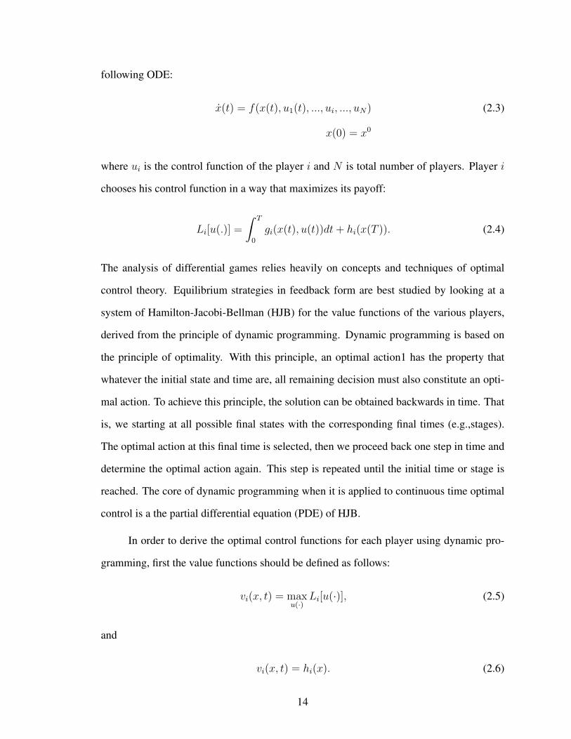
following ODE:
x(t) = f(x(t), u1(t), ..., ui, ..., uN) (2.3)
x(0) = x0
where ui is the control function of the player i and N is total number of players. Player i
chooses his control function in a way that maximizes its payoff:
Li[u(.)] =
ˆ T
0
gi(x(t), u(t))dt+ hi(x(T )). (2.4)
The analysis of differential games relies heavily on concepts and techniques of optimal
control theory. Equilibrium strategies in feedback form are best studied by looking at a
system of Hamilton-Jacobi-Bellman (HJB) for the value functions of the various players,
derived from the principle of dynamic programming. Dynamic programming is based on
the principle of optimality. With this principle, an optimal action1 has the property that
whatever the initial state and time are, all remaining decision must also constitute an opti-
mal action. To achieve this principle, the solution can be obtained backwards in time. That
is, we starting at all possible final states with the corresponding final times (e.g.,stages).
The optimal action at this final time is selected, then we proceed back one step in time and
determine the optimal action again. This step is repeated until the initial time or stage is
reached. The core of dynamic programming when it is applied to continuous time optimal
control is a the partial differential equation (PDE) of HJB.
In order to derive the optimal control functions for each player using dynamic pro-
gramming, first the value functions should be defined as follows:
vi(x, t) = maxu(·)
Li[u(·)], (2.5)
and
vi(x, t) = hi(x). (2.6)
14
For players to play the game, the available information is required. In differential game,
there are three cases of available information.
• Open-loop information: With open-loop action, the players have common knowledge
of the values of state variables at initial time t = 0. At this initial state, each player
chooses the control variable path by taking into account the expected behavior of all
other players. All players commit themselves to their action paths before the game
starts.
• Close-loop information: With close-loop information, players are assumed to know
the values of state variables from time 0 to t, i.e., [0, t) without delay.
• Feedback information: At time t, players are assumed to know the values of state
variables at time t− ϵ, where ϵ is positive and arbitrarily small. The information set
at time t can be estimated from the vector of value of state variables of all players at
time t− ϵ.
At this stage, a natural assumption is that the strategies adopted by players have the
feedback form: ui = u∗i (x
∗); in other words, they depend only on the current state of the
system, not the past history. For a Nash non-cooperative solution in feedback form, one
can show that the value functions, vi, satisfy HJB equations derived from the principle of
dynamic programming.
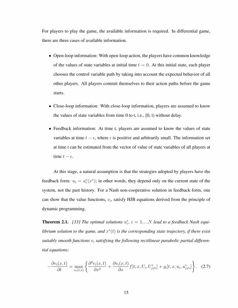
Theorem 2.1. [33] The optimal solutions u∗i , i = 1, ...N lead to a feedback Nash equi-
librium solution to the game, and x∗(t) is the corresponding state trajectory, if there exist
suitably smooth functions vi satisfying the following rectilinear parabolic partial differen-
tial equations:
−∂vi(x, t)
∂t= max
ui(t,x)
{∂2vi(x, t)
∂x2+
∂vi(x, t)
∂xf [t, x, Ui, U
∗j =i] + gi[t, x, ui, u
∗j =i]
}. (2.7)
15
The HJB equation is usually solved backwards in time, starting from t = T and end-
ing at t = 0. In general case, the HJB equation does not have a classical (smooth) solution.
Several notions of generalized solutions have been developed to cover such situations, in-
cluding viscosity solution [35], minimax solution [36]. For the special case of affine-linear
quadratic game, the value function has the unique solution which should satisfy a set of
first order differential equations. The closed form solution for the optimal action can be
obtained for this special case.
2.1.3 Stochastic Differential Games
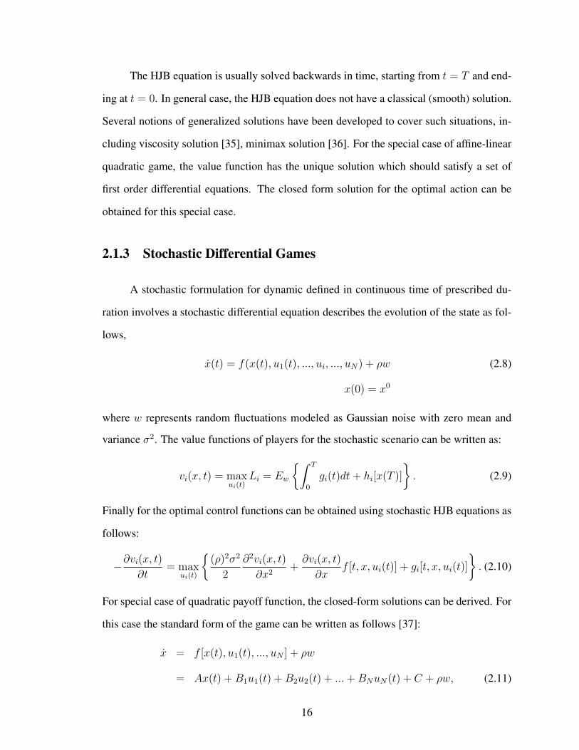
A stochastic formulation for dynamic defined in continuous time of prescribed du-
ration involves a stochastic differential equation describes the evolution of the state as fol-
lows,
x(t) = f(x(t), u1(t), ..., ui, ..., uN) + ρw (2.8)
x(0) = x0
where w represents random fluctuations modeled as Gaussian noise with zero mean and
variance σ2. The value functions of players for the stochastic scenario can be written as:
vi(x, t) = maxui(t)
Li = Ew
{ˆ T
0
gi(t)dt+ hi[x(T )]
}. (2.9)
Finally for the optimal control functions can be obtained using stochastic HJB equations as
follows:
−∂vi(x, t)
∂t= max
ui(t)
{(ρ)2σ2
2
∂2vi(x, t)
∂x2+
∂vi(x, t)
∂xf [t, x, ui(t)] + gi[t, x, ui(t)]
}. (2.10)
For special case of quadratic payoff function, the closed-form solutions can be derived. For
this case the standard form of the game can be written as follows [37]:
x = f [x(t), u1(t), ..., uN ] + ρw
= Ax(t) + B1u1(t) + B2u2(t) + ...+BNuN(t) + C + ρw, (2.11)
16
The affine-quadratic cost function can be rewritten as follows:
gi =1
2Qx2 +Rui
2 +N, (2.12)
hi =1
2Qfx2, (2.13)
Finally, for the value function, we have:
vi(x, t) = maxui(t)
L (2.14)
= maxui(t)
Ew
{ˆ T
0
µ[x(t), ui(t)(t)]dt+ h[x(T )]
}.
According to [33], the value function for an affine linear quadratic problem has a unique
solution for vi(t):
vi[t] =1
2Ti(t)X(t)2 + x(t)ζi(t) + ξi(t) +mi(t), (2.15)
where Ti(t) satisfies the following Riccati differential equations
dTi
dt+ 2TiFi +Qi +
T 2i B
2i
Ri
= 0, (2.16)
Ti(T ) = Qfi , (2.17)
and
Fi = A− TiBi2
Ri
. (2.18)
ζi and mi can be obtained from the following differential equations, respectively:
dζidt
+Fiζi + TiζiBi
2
Ri
+ TiBi = 0, (2.19)
ζi(T ) = 0, (2.20)
dmi
dt+ αiζi +
ζ2i Bi2
2Ri
= 0, (2.21)
17

mi(T ) = 0, (2.22)
αi = C − ζiBi2
Ri
. (2.23)
Finally, ξi statistics the equation below.
dξidt
= −Riσ2ui
2. (2.24)
The optimal control variable can be obtained as follows:
u∗i = −Bi
Ri
∂vi∂x
= −Bi(Tix+ ζi)
Ri
. (2.25)
As it is shown, the optimal control function constitutes a feedback Nash Equilibrium to the
stochastic differential game.
2.2 Overview of Satisfaction Games
In real life distributed systems, agents generally do not have knowledge of their op-
ponents strategies. In this context, most game theoretic solution concepts are hardly appli-
cable. Therefore, it is needed to define equilibrium concepts that do not require complete
information and are achievable through learning, over repeated play. The satisfaction form
is a game theoretical formulation which models systems where players are not interested
in maximizing their own utility, rather in satisfying their own constraints [24].
Let us define the game as
G ′ =(K,AK , {fk}k∈K
), (2.26)
where K and AK follow the previous definitions and the correspondence fk : A(K−1) → A,
called satisfaction correspondence, is defined as
fk(a−k) =
(ak ∈ A :
∑ℓ∈Lk
1{ξℓ(ak,a−k,≥Γ} = Lk
). (2.27)
18

Basically (2.27) is a correspondence which, given the action chosen by the other players,
selects all the actions that satisfy the individual constraints. Here, a player can use any of
its actions independently of all the other players. The dependence on the other players’
actions plays a role only in determining whether a player is satisfied or not.
In this game formulation, the solution concept we adopt is the satisfaction equilib-
rium (SE) [24] defined as follows:
Definition 2.2. (Satisfaction equilibrium). A satisfaction equilibrium of game G ′ is an
action profile a′ ∈ AK such that ∀k ∈ K,
a′k ∈ fk(a′−k
). (2.28)
The SE is an action profile where all players are simultaneously satisfying their con-
straints. In other words, if there exists at least one SE, then L∗ = L, since all players can
be satisfied. However, an SE does not always exist for a given game. For instance, if not
all the communications can simultaneously take place with the minimum required QoS in
the network modeled by the game G, an SE simply does not exist. An extensive discussion
on the existence and multiplicity of an SE in finite games is provided in [25].
2.2.1 Efficient Satisfaction Equilibrium
Consider that player k assigns a cost to each of its actions ak, which we denote by
ck(ak). For all k ∈ K, the cost function ck : Ak → [0, 1] satisfies the following condition:
∀(ak, a′k) ∈ A2k, it holds that
ck (ak) < ck (a′k) , (2.29)
if and only if, ak requires a lower effort than action a′k when it is played by player k. In
the QoS problem, the effort can be associated with the transmit power or the processing
time required to implement a given transmit/receive configuration [26]. Thus, considering
the effort or cost of individual actions, one SE which is particularly interesting in the QoS
provisioning problem is the one that requires the lowest individual effort.
19

Definition 2.3 (Efficient Satisfaction Equilibrium). An action profile a∗ is an ESE for the
game G, with cost functions {ck}k∈K, if for all k ∈ K,
(i) a∗k ∈ fk(a∗−k
)and (2.30)
(ii) ∀ak ∈ fk(a∗−k), ck(ak) ≥ ck(a
∗k). (2.31)
The effort associated by each player with each of its actions does not depend on the
choices made by other players. Thus, an ESE a∗ ∈ A, if it exists, is one SE at which player
k is satisfied by using the action a∗k that requires the minimum effort among all the actions
in fk(a−k). Nonetheless, the existence of an SE does not imply the existence of an ESE.
2.2.2 Modeling Drop-ins and Drop-outs
Consider a game played only by a subset J ⊂ K of the players of the game G and
denote it by
G(J ) =
(J , {Ak}k∈J ,
{f(J )k
}k∈J
). (2.32)
The function f(J )k : AJ → 2Ak determines the set of actions that satisfy the individual
constraints of player k given the actions adopted by the subset of players J . In the game
G(J ), players in K \ J do not play any role in the decisions adopted by the players in J .
More precisely, the game G(J ) is obtained when the players in the set K\J have decided
to drop out of the original game G [27].
A player j drops out of the game G by playing the action corresponding to a standby
state of the link which is denoted by A(0)j . In the game G, such an action A
(0)j satisfies the
following condition for all j ∈ J :
f(J )k (aJ\{j}) = fk
(aJ\{j},A
(0)K\J
), (2.33)
where the action profile A(0)K\J represents an action profile in which all players k ∈ K \ J
use the action A(0)k .
20

The equality in (2.33) shows that when a set of players K \ J choose to play their
actions A(0)k in the game G, they do not play any role in the choice of the actions of the
players in J .
The relevance of a game G(J ), given a set J ⊆ K, stems from the fact that if the
game G does not have an SE, the set J can be chosen in order to allow the satisfaction
of the largest population of players. That is, J can be constructed such that the sub-game
G(J ) is the game with the largest population that possesses an SE. We refer to these action
profiles as N -Person Satisfaction Points (N -PSPs) of the game G.
Definition 2.4 (N -Person Satisfaction Point (N -PSP)). Assume the game in satisfaction
form G does not possess an SE. Then, an action profile (a∗J ,A
(0)K\J ) is said to be an N -PSP,
if |J | = N and G(J ) =
(J , {Ak}k∈J ,
{f(J )k
}k∈J
)is the sub-game with the largest set
of players that has an SE.
When a game G possesses at least one SE, any SE is a K-PSP. That is, when the si-
multaneous satisfaction of all individual constraints is feasible, SE and K-PSP are identical
notions.
21

Chapter 3
Stochastic Dynamic Hydrothermal Scheduling ina Smart Grid network
3.1 Introduction
Recent efforts on smart grids [1–3,13–15,28] are motivated in part by the increasing
demand for electric power, growing interest in finding pollution-free and sustainable energy
supply sources, and inadequacy of the current transmission system. Energy storages can
balance supply and demand of the electricity market, and mitigate supply side uncertainties.
Among grid energy storages, pumped-storage plants generally have the largest available
capacity. A pumped storage plant stores off-peak energy using water which is later used
for generation during peak periods. Other types of energy storing devices and plug-in
electrical vehicles have limited use in power systems due to their relatively small capacity
and high costs.
Pumped-storage plants are usually operated within an overall system which contains
thermal generation due to very high operating cost of thermal power plants compared to the
operating cost of hydro power plant. The hydrothermal generation scheduling is concerned
with both hydro plant scheduling and thermal plant dispatching. A variety of optimization
methods have been proposed for planning the optimal operations of hydrothermal power
systems. The scheduling problems considering deterministic and stochastic programming
models have been studied for different time horizons. The planning horizons considered
are long-medium term (1 to 3 years) [38–40], or short-term (weeks to a day) [41, 42]. For
short-term models, the optimal operation scheduling of the available generating plants is
defined for the following 24 hours. Specifically, authors in [43] introduced the stochastic
programming models for the short-term hydro-thermal scheduling problem under uncertain
demand. Authors in [44] developed the stochastic scheduling models for the short-term
22

hydropower production considering the uncertainty of natural inflows in reservoirs.
A widely used paradigm for modeling the hydrothermal power plants behavior in the
oligopolistic electricity markets is so called the Nash-Cournot model, dealing with the anal-
ysis of the market equilibria [45]. The Nash-Cournot approach assumes that each strategic
power plants decides its generation level supposing the energy outputs by the remaining
strategic power plants are known. The market scheme is thus simulated through a game: the
first strategic power plant chooses its profit-maximizing output under the assumption that
the production of the other strategic power plants is known. This is repeated for each strate-
gic power plant that decides its generation level based upon the most recent decisions of the
others, until reaching a Nash equilibrium, where no power plant can profit from changing
its output levels given the output of all other strategic power plants [46]. In [47], some
theoretical results concerning the Cournot model applied to short-term electricity markets
are presented. Authors in [48] address a short term hydrothermal scheduling problem using
differential dynamic programming but not in a game fashion. The problem is decomposed
into a thermal subproblem and a hydro subproblem that are solved in parallel through a
constraint relaxed iterative algorithm not in a game fashion. A hydrothermal power ex-
change market that incorporates network constraints is proposed in [49], the Nash-Cournot
equilibrium solution of the market is achieved using the Nikaido-Isoda function, which is
derived from the profit maximization functions calculated by the generating companies.
The reservoir dynamic is not incorporated in the system model.
In this chapter, we study the competitive interactions between an autonomous pumped-
storage hydropower plant and a thermal-power plant in order to optimize power genera-
tion and storage. The instantaneous market price can be modeled as a Cournot duopoly
game [29, 30]. Here, the dynamic comes from the water volume in the reservoir, and the
stochastic captures the natural inflow and loss to the reservoir. The hydro plant decides
how much power to produce, and the thermal plant decides how much to sell to the market
or sell to the hydro plant for pump-up storage. The major contributions of this paper are:
23

• We propose a game-theorical framework in which the thermal and pumped-storage
power plants are networked and the thermal plant has the choice to sell the power to
the pumped-storage plant.
• We solve the stochastic the Hamilton–Jacobi–Bellman (HJB) equation and obtain an
optimal closed-form solutions for both thermal and hydro players.
• We analyze the outcome of interactions between two players and prove it constitutes
a feedback Nash equilibrium solution.
• We demonstrate through simulations that the proposed framework can reduce the
peak to average ratio and total energy generation of the thermal plant, which help
plant operation and reduce CO2 emission with respect to the case that hydro and
thermal power plants are working in isolation.
The rest of this chapter is organized as follows: In Section 3.2, the system model
is given, and the game is constructed. In Section 3.3, we study the close-form solutions
and properties of the proposed game. Simulation results are shown in Section 3.4. Fi-
nally, conclusions are drawn in Section 3.5. For better readability, important variables and
parameters used in this paper are listed in Table 3.1.
3.2 System Model and Game Formulation
We consider a smart grid network with one pumped-storage hydro power plant and
one thermal power plant as two price makers. Each price maker power plant has autonomy
to maximize its own profit by adjusting its generation volume. The power can be sold in the
market, and the unit power price depends on the demand and supply, and is dynamic over
different periods of time. Alternatively, the thermal power plant can sell its power at a fixed
price to the pumped-storage hydro plant by storing the energy in the reservoir. The state
of available hydroelectric energy depends on the amount of water stored in the reservoirs.
24

Table 3.1 Variables and parameters for system model
Symbol Descriptionx reservoir volumerH water discharge ratesH water spillage ratepgT thermal plant output to sell to the marketpsT thermal plant output to storepH pumped-storage outputw natural inflows to the storageD the total demandβ storage leakage rateη1 turbine efficiencyη2 generator efficiencyg acceleration of gravityp market priceK fixed price from thermal to hydro
The uncertainty of natural inflows and outflows to the reservoir is modeled as stochastic
processes. The overall system model is illustrated in Figure 3.1.
Based on the system setup, a quantitative 2-player differential game is defined with
the following components1: A time interval [0, T ] is specified a priori and denotes the
duration of the evolution of the game. In this paper, [0, T ] represents each hour in a one-
day duration. An infinite set with some topological structure is defined for each power plant
and is called the action space, whose elements are the control functions. For the pumped-
storage hydro plant the action u1(t) = rH(t) is the discharged water from the dam; and
for the thermal plant, the action u2(t) = pgT (t) is how much power to sell to the market
from its output. Notice that we define u1 and u2 here since the definitions will make the
analysis clear in the following sections. The actions of the power plant and thermal plant
will affect the market price as well as the storage volume in the reservoir. The goal is to
study the optimal strategies to control the actions, and analyze the interaction between the
two plants.
1In this paper, we consider a two-player game, and multiple price maker player games will be studied inour future study.
25
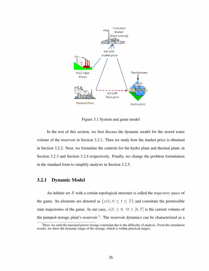
Figure 3.1 System and game model
In the rest of this section, we first discuss the dynamic model for the stored water
volume of the reservoir in Section 3.2.1. Then we study how the market price is obtained
in Section 3.2.2. Next, we formulate the controls for the hydro plant and thermal plant, in
Section 3.2.3 and Section 3.2.4 respectively. Finally, we change the problem formulation
in the standard form to simplify analysis in Section 3.2.5.
3.2.1 Dynamic Model
An infinite set X with a certain topological structure is called the trajectory space of
the game. Its elements are denoted as {x(t), 0 ≤ t ≤ T} and constitute the permissible
state trajectories of the game. In our case, x(t) ≥ 0, ∀t ∈ [0, T ] is the current volume of
the pumped-storage plant’s reservoir 2. The reservoir dynamics can be characterized as a
2Here, we omit the maximal power storage constraint due to the difficulty of analysis. From the simulationresults, we show the dynamic range of the storage, which is within practical ranges.
26

linear differential equation [48]:
dx(t)
dt= −ρ0βx(t) + ρ1p
sT (t) + ρ2(w − ϑH), (3.1)
where x is the reservoir volume in (m3), β is reservoir leakage rate, ρ0, ρ1 and ρ2 are
the constant factors, w represents random fluctuations modeled as Gaussian noise with
zero mean3 and variance σ2. In addition, pT is the total power generated by the thermal
plant and psT represents the amount power that the thermal plant decides to store. We
assume the initial state x0 is known. It is important to note that, this dynamic model of
reservoir is applicable to the normal operation of the pumped-storage power plant and does
not consider extreme cases, such as dead storage level or flooding condition. Alternatively
boundary conditions can be coped by adding barrier functions [29]. However, there will
be no closed-form solution as derived in the sequel and only numerical solutions can be
obtained.
Since the generation of the thermal power plant has a slow response to load changes,
for simplicity, we assume pT = pgT (t) + psT (t) to be constant in this paper. If pT changing
slowly over time, a similar approach applies. Finally, the total water released at time t is
shown by ϑH(t) which can be obtained as:
ϑH = rH + sH , (3.2)
where rH is the water discharge rate in (m3/s), and sH is water spillage rate in (m3/s)
assumed to be constant over time. 4 The pumped-storage power plant generation at time t,
pH(t), can be estimated as [51]:
pH(t) = η(x(t))rh(t), (3.3)
where η is function of the net head or, equivalently, the volume of the stored water in the
reservoir. Since x and rH perturbations are small compared with the normal values of these3non-zero mean case can be studied by adding a constant in (3.1).4In practice, spillage rate is not a constant. However, we can model the randomness together with w.
27

parameters (operating point) for large reservoirs, the linear small disturbance approxima-
tion [52] can be used to write the hydro generation as:
pH(t) = W1rH(t) +W2x(t) = W1u1(t) +W2x(t). (3.4)
Let the operating point be (x†, rh†), W1 and W2 can then be computed as follows [52]:
W1 = gη1η2x†, (3.5)
W2 = gη1η2rh†. (3.6)
Replacing equations (3.2) and (3.4) in equation (3.1), the storage dynamic equation
can be rewritten as function of the system state and control variables as follows:
dx(t)
dt= f [x(t), u1(t), u2(t)]dt+ ρ2w (3.7)
= {−ρ0βx(t) + ρ1[pT − pgT (t)]− ρ2{rH(t) + sH}}+ ρ2w.
3.2.2 Market Price Model
Using the market price model introduced in [45], we assume the price takers have a
quadratic operating cost
C(O) =O2
2α, (3.8)
where O is total generation of price taker power plants and α is a scalar parameter. Using
this assumption, given a market spot price p, the price taker plant generation can be obtained
by setting their marginal generation cost equal to the market price. The marginal generation
cost can be obtained the derivative of with respect to O. Therefore, the price taker plants
generation is a linear function of the spot price p, i.e., O(p) = αp.
Consider D as the total demand, and O(p) as the total generation of price takers as
discussed above. The total output of price maker power plants, pH(t)+pgT (t), should satisfy
28

the residual demand:
Dr = D −O(p) = D − αp. (3.9)
Therefore, the spot price can be obtained as:
p = {D − [pH(t) + pgT (t)]}/α. (3.10)
Without loss of generality, we assume α = 1 in the rest of paper for simplicity.
3.2.3 Control for Hydro Plant
The revenue of the hydro plant, given the generation of other plants as given is:
g1(t) = [D − pH(t)− pgT (t)] pH(t)−KpsT (t), (3.11)
where the first term in (3.11) is the profit of selling power to the market, and the second
term is the cost that the thermal player sells to the hydro player to store the power in the
reservoir (by pumping water up). Here K represents the constant price (e.g. per a long-
term contract) for selling from the thermal player to the hydro player. We can rewrite (3.11)
with state (x(t)) and control (u1(t) and u2(t)) as
g1(t) = {D −W1u1(t)−W2x(t)− u2(t)} [W1u1(t) +W2x(t)]−K[pT − u2(t)].(3.12)
The stochastic dynamic game of the pumped-storage hydro player is to control its
discharged water rH so as to maximize the following utility over the time interval
v1(x) = maxu1(t)=rH(t)
L1 = Ew
{ˆ T
0
g1(t)dt
}. (3.13)
3.2.4 Control for Thermal Plant
Similarly, the stochastic dynamic game of the thermal player is to control its selling
u2(t) = pgT (t) and storing psT so as to maximize its utility. Since we assume pT to be
29

a constant, the thermal plant’s action can be uniquely determined by u2(t). The thermal
plant tries to maximize the following:
g2(t) = {D − pH(t)− pgT}pgT (t) +KpsT (t){ϵ2p2T + ϵ1pT + ϵ0}, (3.14)
v2(x) = maxu2(t)=pgT (t)
L2 = Ew
{ˆ T
0
g2(t)dt
}. (3.15)
In (3.14), the first term is the profit to sell in the market, the second term is the profit to sell
to the hydro player, and the third term is the power generation cost [53]. Here ϵ0, ϵ1 and ϵ2
are constants. We can rewrite (3.14) as
g2(t) = {D −W1u1(t)−W2x(t)− u2(t)}u2(t) +K[pT − u2(t)]− {ϵ2p2T + ϵ1pT + ϵ0}.(3.16)
3.2.5 Standard Form Notation
Table 3.2 Change of variables table
X 3W2x√2
+P [e]−ug
T
2√3
U1 W1rH + W2x2
+P [e]−ug
T
2
U2 ugT − D−(W1rH
∗+W2x)−K2
A 5ρ0β−ρ1W2−3ρ2W2
−4W2(3√2+ 1
4√
3)
B1−√2ρ0β−6
√3ρ1W2+(
√2−12
√3)ρ2W2
−W2(12√3+
√2)
B22ρ0β+12
√3ρ1W2+(
√2+6
√3)ρ2W2
−W2(12√3+
√2)
C ρ1uT −ρ2sH+ P [e](A+√3B1−
√3B2)
2√3
+B2K2
QH ,RH 2QT ,Qf
H ,QfT , 0
NH −KusT − (D−ug
T∗)2
3
RT -1NT KuT − {ϵ2[ug
T (t) + usT (t)]
2 +ϵ1[u
gT (t) + us
T (t)] + ϵ0} +(D−(W1rH
∗+W2x∗)−K)2
4
Notice that the utility functions are not in a standard form of the controls. So we
change the variables as shown in Table 3.2. By changing the variable, the problem in (3.7)
30

is an affine-quadratic differential game [33] with dynamics in the form of5
dX
dt= f(X,U1, U2)dt+ ρ2w = (AX +B1U1 +B2U2 + C) + ρ2w. (3.17)
From (3.12) and (3.14), the pumped-storage and thermal plants payoff functions are, re-
spectively, in forms of
g1 =1
2QHX
2 +RHU12 +NH , (3.18)
h1 =1
2Qf
HX2, (3.19)
and
g2 =1
2QTX
2 +RTU22 +NT , (3.20)
h2 =1
2Qf
TX2. (3.21)
In summary, the pumped-storage plant and thermal plant control u1(t) = rH(t) and
u2(t) = pgT (t), respectively. The dynamics in (3.17) is a linear function of state x(t) and
those two controls, and the utility functions are in the linear quadratic forms of the controls.
3.3 Game Analysis and Performance
As an overview, differential games are the extension of the optimal control problems
[33]. The Nash feedback equilibrium strategies are derived from a system of The Hamilton-
Jacobi-Bellman (HJB) equations for the value functions of the players. The solution is
obtained backwards in time using dynamic programming. That is, starting from all possible
final states, the optimal action at each final time is selected, we then induce backward one
step at time and determine the optimal action at each stage. This process is repeated until
the initial time or stage is reached.
5for notational simplicity time index t is omitted
31
In this section we analyze the nonzero sum stochastic differential game of the thermal
and pumped-storage power plants based on the models in the previous section. In the
sequel, we will study the payoff maximization of pumped-storage plant and thermal plant
given the other’s strategy is fixed in Section 3.3.1 and Section 3.3.2, respectively. Finally,
we discuss the outcome of the proposed games in Section 3.3.3.
3.3.1 Pumped-Storage Player Payoff Maximization
First, given the thermal plant’s strategy, the pumped-storage plant calculates its the
best strategy through the stochastic HJB equation. This equation is considered to be the
first-order necessary and sufficient condition obeyed by the optimal value function and can
be used to find the optimal time paths of the state, costate, and control variables. If the
HJB equation is solvable (either analytically or numerically), an optimal feedback control
can be obtained by taking the maiximizer involved in the HJB equation [33]. To optimize
the utility function in (3.13), the HJB equation for the pumped-storage power plant can be
written as follows:
−∂v1∂t
= maxU1
{(ρ2)
2σ2
2
∂2v1∂X2
+∂v1∂X
f(X,U1, U2∗) + g1
}, (3.22)
v1[X(T )] = h1[X(T )]. (3.23)
In order to obtain the optimal action for each player of game, first the related value
functions have to be derived, for the special case of affine-linear quadratic game, the value
function has the unique solution [33] which should satisfy a set of first order differential
equations. The closed form solution for the optimal action of hydro plant is presented
through the following lemma.
Lemma 3.1. Using the HJB equation, the optimal control policy for the pumped-storage
hydro plant can be obtained as:
U∗1 = − B1
RH
∂v1∂X
= −B1(THX + ζH)
RH
. (3.24)
32

Proof. The value function of the hydro player can be written as:
v1[t] =1
2TH(t)X(t)2 +X(t)ζH(t) + ξH(t) +mH(t), (3.25)
where TH(t) satisfies the following Riccati differential equations [33]
dTH
dt+ 2THFH +QH +
T 2HB
21
RH
= 0, (3.26)
TH(T ) = QfH , (3.27)
and
FH = A− THB12
RH
. (3.28)
ζH and mH can be obtained from the following differential equations, respectively:
dζHdt
+FHζH + THζHB1
2
RH
+ THB1 = 0, (3.29)
ζH(T ) = 0, (3.30)
dmH
dt+ αHζH +
ζ2HB12
2RH
= 0, (3.31)
mH(T ) = 0, (3.32)
αH = C − ζHB12
RH
. (3.33)
Finally, ξH satisfies the equation below.
dξHdt
= −RHσ2U1
2. (3.34)
The optimal control variable can be obtained as follows:
U∗1 = − B1
RH
∂v1∂X
= −B1(THX + ζH)
RH
. (3.35)
33

3.3.2 Thermal Player Payoff Maximization
Next, we determine the optimal strategy of the thermal plant given the optimal strat-
egy of the hydro plant. To optimize the utility in (3.15), the stochastic HJB equation of the
proposed game for the thermal player can be represented by following equation
−∂v2∂t
= maxU2
{(ρ2)
2σ2
2
∂2v2∂X2
+∂v2∂X
f(X,U1∗, U2) + g2
}, (3.36)
v2[X(T )] = h2[X(T )]. (3.37)
The optimal action for the thermal plant can be obtained through the following lemma.
Lemma 3.2. The optimal control policy for the thermal plant can be obtained as follows:
U∗2 = −B2
RT
∂v2∂X
= −B2(TTX + ζT )
RT
. (3.38)
Proof. The value function of thermal player can be written as:
v2[t] =1
2TT (t)X(t)2 +X(t)ζT (t) +X(t)ξT (t) +mT (t). (3.39)
Here, TT (t) satisfies the following Riccati differential equations [33]
dTT
dt+ 2TTFT +QT +
TT2B2
2
RT
= 0, (3.40)
TT (T ) = QfT , (3.41)
FT = A− TTB22
RT
. (3.42)
ζT and mT can be obtained through similar steps in (3.29)-(3.34):
dζTdt
+FT ζT + TT ζTB2
2
RT
+ TTB2 = 0, (3.43)
ζT (T ) = 0, (3.44)
34
dmT
dt+ αT ζT +
ζ2TB22
2RT
= 0, (3.45)
mT (T ) = 0, (3.46)
αT = C − ζTB22
RT
, (3.47)
and ξT from the equation below.
dξTdt
= −RTσ2U2
2. (3.48)
The optimal control variable can be obtained as follows:
U∗2 = −B2
RT
∂v2∂X
= −B2(TTX + ζT )
RT
. (3.49)
3.3.3 Nash Equilibrium
For a two-person differential game in the form discussed in the previous subsections,
a two-tuple strategies constitutes a feedback Nash equilibrium solution [33] as defined
below:
Definition 3.3. A set of controls U∗i (t,X), i ∈ 1, 2 constitute a feedback Nash equilibrium
of the game, if there exists functions vi(X, t) satisfying the following relations ∀i :
vi(X, t) = Ew
[ˆ T
0
gi{t,X∗(t), U∗1 [t,X(t)], U∗
2 [t,X(t)]}dt]
(3.50)
≥ Ew
[ˆ T
0
gi{t,X [i](t), Ui[s,X(s)], U∗j =i[t,X(t)]}dt
],
where
dX [i](t)
dt= f{t,X [i](t), Ui[t,X(t)], U∗
j =i[t,X(t)]} (3.51)
35
and
dX∗(s)
dt= f{t,X∗(t), U∗
1 [t,X(t)], U∗2 [t,X(t)]}. (3.52)
If there exists the value functions that are twice continuously differentiable, then
the two partial differential feedback Nash equilibrium solutions in continuous time can be
characterized using the stochastic HJB equations [33], which are necessary conditions of
the candidate optimal control strategy. The feedback Nash equilibrium is defined as follows
(Theorem 6.27 [33]):
Theorem 3.4. A set of feedback strategies U∗i (t,X
∗) lead to a feedback Nash equilibrium
solution to the game, and X∗(t), 0 ≤ t ≤ T is the corresponding state trajectory, if there
exist suitably smooth functions Vi satisfying the following rectilinear parabolic partial dif-
ferential equations:
−∂vi(X, t)
∂t= max
Ui(t,X){(ρ2)
2σ2
2
∂2vi(X, t)
∂X2(3.53)
+∂vi(X, t)
∂Xf [t,X, Ui, U
∗j =i] + gi[t,X, Ui, U
∗j =i]}.
Lemma 3.5. The feedback Nash equilibrium exists for the proposed game in (3.17), (3.18),
(3.19), (3.20), and (3.21).
Proof. Since the value functions in equations (3.25) and (3.39) are twice continuously dif-
ferentiable, the derived optimal solution by HJB equations characterize the feedback Nash
equilibrium solutions.
3.4 Simulation Results
In this section, to clarify the game analysis results derived in Section 3.3, we inves-
tigate the performance of the proposed game numerically. The simulations are performed
36
2 4 6 8 10 12 14 16 18 20 22 240
2
4
6
8
10
12x 10
5
Time (Hour)
D(t)Price per Watt
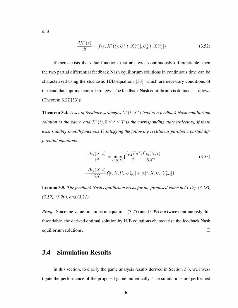
Figure 3.2 Daily demand D(t) versus market price based on data from [57]
for each hour in a one-day duration. The thermal and pumped-storage plants have the max-
imum generation capacities of 500MW and 300MW , respectively. Other parameters are
set as follows: β = 0.05, ρ0 = 3.4∗10−4, ρ1 = 3.83∗10−5, ρ2 = 0.001, σ2 = 0.5, η1 = 0.9,
η2 = 0.96, x† = 550Mm3, rh† = 103∗10−1m3
s, xmax = 717Mm3 and ϵ2 = ϵ1 = ϵ0 = 0.5.
The above characteristic values for the hydro plant’s reservoir are selected based on [56].
The constant price K for thermal player to sell to the hydro player is assumed to be equal
to 100000, unless we otherwise define. Figure 3.2 shows fluctuations of total demand D
according to [57], and how the market price per Watt ({D − pH(t)− pgT (t)}) is affected
accordingly. Notice that the market price can be affected by many other players in the mar-
ket. Here we consider only the thermal and hydro players so that the interactions can be
clearly demonstrated.
In Figure 3.3, the pumped-storage plant generation amount (pH) and thermal plant
generation decision (pgT ) are compared over time. The amount of generation of the thermal
plant and pumped-storage plant both follow the fluctuations of demand. However, com-
pared with the demand in Figure 3.2, the thermal player has less fluctuation, and the hydro
(pumped storage plant) player compensates for the fluctuation. This can help practical op-
37

2 4 6 8 10 12 14 16 18 20 22 24150
200
250
300
350
400
450
500
Time (Hour)
Pow
er (
MW
att)
Thermal, K=300000Pumped−Storage, K=300000Thermal, K=200000Pumped−Storage, K=200000Thermal, K=100000Pumped−Storage, K=100000
Figure 3.3 Comparison of the output power of the thermal plant and the pumped-storageplant to sell to the market for different amounts of K
erations since the thermal player has a slow response to meet the demand’s fluctuations.
Also, we change the price per Watt of the electricity that the thermal plant sells power to
the pumped-storage plant, K from 100000 to 300000. By increasing K the thermal plant
finds selling its output power to the pumped-storage plant more beneficial than selling it to
the market. Therefore, the amount of power that the thermal plant generates for selling to
the market decreases and the generation of pumped-storage plant increases, respectively to
satisfy the demand.
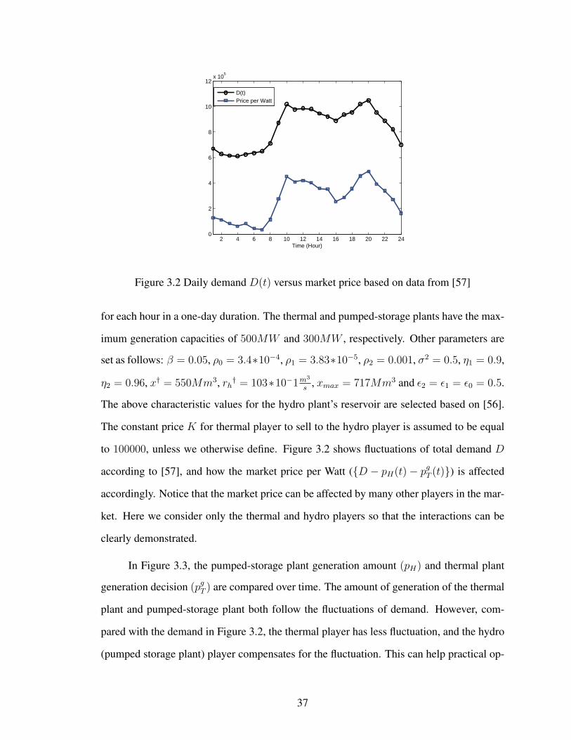
The reservoir volume and water discharge rate of the pumped-storage plant in each
hour is shown in Figure 3.4. Comparing with Figure 3.3, the reservoir volume varies with
the generation value of the pumped-storage plant. For instance when the plant decides to
increase its output power, the discharge rate increases and the reservoir level decays. When
K increases, the volume drops and the discharge rate increases. Moreover, notice that the
power generation is a function of both reservoir volume and water discharge rate.
In Figure 3.5, the payoffs of power plants from equations (3.11)-(3.14) are compared
for different values of K. For all scenarios, the variations of the payoff functions are
38
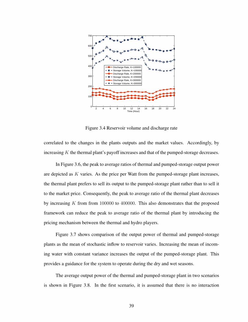
2 4 6 8 10 12 14 16 18 20 22 240
100
200
300
400
500
600
700
Time (Hour)
Discharge Rate, K=100000Storage Volume, K=100000Discharge Rate, K=200000Storage Volume, K=200000Discharge Rate, K=300000Storage Volume, K=300000
Figure 3.4 Reservoir volume and discharge rate
correlated to the changes in the plants outputs and the market values. Accordingly, by
increasing K the thermal plant’s payoff increases and that of the pumped-storage decreases.
In Figure 3.6, the peak to average ratios of thermal and pumped-storage output power
are depicted as K varies. As the price per Watt from the pumped-storage plant increases,
the thermal plant prefers to sell its output to the pumped-storage plant rather than to sell it
to the market price. Consequently, the peak to average ratio of the thermal plant decreases
by increasing K from from 100000 to 400000. This also demonstrates that the proposed
framework can reduce the peak to average ratio of the thermal plant by introducing the
pricing mechanism between the thermal and hydro players.
Figure 3.7 shows comparison of the output power of thermal and pumped-storage
plants as the mean of stochastic inflow to reservoir varies. Increasing the mean of incom-
ing water with constant variance increases the output of the pumped-storage plant. This
provides a guidance for the system to operate during the dry and wet seasons.
The average output power of the thermal and pumped-storage plant in two scenarios
is shown in Figure 3.8. In the first scenario, it is assumed that there is no interaction
39

2 4 6 8 10 12 14 16 18 20 22 240
0.5
1
1.5
2
2.5
3
3.5
4x 10
11
Time (Hour)
Pay
off
Pumped−Storage, K=300000Thermal, K=300000Pumped−Storage, K=200000Thermal, K=200000Pumped−Storage, K=100000Thermal, K=100000
Figure 3.5 Comparison of thermal and pumped-storage plants payoffs to sell to the marketfor different amounts of K
between two power plants, and they just sell their outputs to the market (K = 0). In
the second scenario, plants are networked with suggested price from pumped-storage plant
(K = 200000). It can be seen that the later case, increases the participation of pumped-
storage plant in demand satisfaction and reduces the thermal’s one, which yields a greener
choice compared to the first scenario.
3.5 Summery
In this chapter, we studied the problem of optimal generation and storage for two
types of competitive power plants in smart grid networks. We have proposed a stochas-
tic dynamic game approach to model their competition. The market price is based on
the Cournot duopoly game model. The thermal power player can sell its power to the hy-
dropower player at a fixed price or to the market at the market price. Based on the stochastic
HJB equation, we derive the strategies for both players if the other’s action is fixed. We
showed that there exists the feedback Nash equilibrium strategies for the proposed game.
40

1 2 3 4
x 105
0
0.5
1
1.5
2
2.5
3
K
Pea
k to
Ave
rage
Rat
io
Pumped Storage PlantThermal Plant
Figure 3.6 Comparison of output power peak to average ratio of thermal and pumped-storage plants for different amounts of K
Simulation results demonstrate the properties of the proposed game and suggest how the
two types of power plants need to adjust their generating and storage decision variables to
maximize their revenues. It is demonstrated that the proposed framework and games can
reduce the peak to average ratio and total energy generation for the thermal plant, which
helps power plant operation and reduces CO2 emission.
41
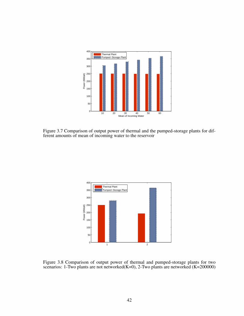
10 20 30 40 50 600
50
100
150
200
250
300
350
400
Mean of Incoming Water
Pow
er (
MW
att)
Thermal PlantPumped−Storage Plant
Figure 3.7 Comparison of output power of thermal and the pumped-storage plants for dif-ferent amounts of mean of incoming water to the reservoir
1 20
50
100
150
200
250
300
350
400
Pow
er (
MW
att)
Thermal PlantPumped−Storage Plant
Figure 3.8 Comparison of output power of thermal and pumped-storage plants for twoscenarios: 1-Two plants are not networked(K=0), 2-Two plants are networked (K=200000)
42

Chapter 4
Distributed Dynamic Control for SmartBuildings
4.1 Introduction
Demand Response (DR) programs are implemented by utility companies to control
the energy consumption at the customer side of the meter. Two popular DR approaches are
direct load control (DLC) and smart pricing. In DLC [60–63], an aggregator can remotely
control the operations and energy consumption of certain consumer appliances. In contrast,
in smart pricing, users are encouraged to individually and voluntarily manage their load,
e.g., by reducing their consumption at peak price hours. This can be done using automated
Energy Consumption Scheduling (ECS) devices [64]. For each user, the ECS finds the best
load schedule to minimize the user’s electricity cost while fulfilling the user energy needs.
This can lead to autonomous demand response programs that burden a minimal control
overhead on utilities.
A common analytical tool to study autonomous DR systems is game theory [65], that
provides a framework to study rational interactions and outcome in a distributed manner. In
[66], a stochastic game is developed to model an hourly energy auction in which generators
and consumers participate as adaptive agents.
In [67], authors proposed a game theoretic demand response scheme to replace tra-
ditional centralized load prediction with a distributed load prediction system that involves
user participation. Authors in [68] employed the Cournot game model to analyze the mar-
ket effect of a demand response aggregator on both shifting and reducing deferrable loads.
Authors in [69] developed a hybrid day-ahead and real-time consumption scheduling for a
number of houses that participate in a demand side program based on game theory. The
43

interaction between the service provider and the users is modeled as a Stackelberg game
in [70] to derive the optimal real-time electricity price and each user’s optimal power con-
sumption. In [71], a residential energy consumption scheduling framework is proposed,
which attempts to achieve a desired trade-off between minimizing the electricity payment
and minimizing the waiting time for the operation of household appliance in presence of
real-time prices using price prediction. In [72], game theory is used for demand side man-
agement to reduce the peak-to-average-ratio in aggregate load demand. In [30], a tutorial
is given for the game-theoretic methods on microgrid systems, demand-side management,
and smart grid communications.
Different from the prior work in [66]- [30], in this paper, we focus on game-theoretic
analysis of price-based DR programs where controllable load types are associated with
dynamic systems and can be modeled using differential equations. Examples of such loads
include heating, ventilation, and air conditioning (HVAC), water heating, refrigeration, and
plug-in electric vehicles. In particular, we apply techniques from stochastic differential
games [33]. To the best of our knowledge, this paper is the first work to study differential
games in the context of price-based DR programs. The contributions in this chapter can be
summarized as follows:
1. We study the strategic interactions between a Nash Cournot electricity market and
multiple energy-smart buildings to construct a two-level stochastic differential game
framework. At the upper level, the market offers a vector of hourly prices to end
users. At the lower level, the energy-smart buildings as the lower level participate
in demand response by managing controllable dynamic load in response to hourly
prices set by the market.
2. We focus on smart buildings equipped with renewable resources generators, local
energy storage and controllable HVAC units, in which users are able to respond to
real-time grid conditions like electricity prices and weather conditions in order to
44
minimize their cost.
3. We derive the optimal closed-form control strategies for each energy-smart building
obtained by solving stochastic the Hamilton-Jacobi-Bellman (HJB) equation. We
analyze the outcome of interactions between two levels and constitute a feedback
Nash equilibrium solution.
4. The proposed technique comparing with the day-ahead pricing method, makes the
load profile more flat and reduces the peak-to-average ratio (PAR) of aggregate load.
5. Using simulation results we show that by implementing our proposed stochastic dif-
ferential DR game model, we can minimize the electricity cost of buildings.
The rest of this chapter is organized as follows. The system model is described in
Section 4.2. The stochastic differential game is constructed and it solution to the proposed
game is derived in Section 4.3. Simulation results are presented in Section 4.4. Conclusions
are drawn in Section 4.5.
4.2 System Model
In this section, we explain the system model that incorporates the impact of demand
response on both supply and demand sides when real-time pricing is used. As illustrated in
Figure 4.1, we study a two-level design framework: at the upper level, at the beginning of
each time interval, e.g., at each hour, the market decides on a price to pass on to the end-
users in the lower level, based on the total demand data from the lower level during the last
time interval. The ECS unit of each building minimizes the cost of electricity consumption.
Since there are multiple buildings competing for the electricity resources, the system can
be analyzed using game theory [65].
45
4.2.1 Smart Building Consumers
Consider a total of N energy-smart buildings that participate in demand response
program. Each building has two specific controllable loads: an air conditioner with a
controllable thermostat, and an always-connected battery. We also assume that a renewable
source of energy, e.g., a residential wind turbine or a roof-top solar panel, is available in
each building, with its generated output to be used to charge the battery. Uncontrollable
appliances with a total and known consumption of l(t) constitute the rest of the building
power consumption. Given the price that is a function of the optimal strategy of the upper
level player, the decision variables available for consumers at each building i = 1, . . . , N
are:
ui1 = power draw from battery for home usage,
ui2 = air conditioner usage of electricity.
And the dynamic states include:
xi1 = the energy stored in the battery array,
xi2 = the indoor temperature of home.
The output power of the renewable generator is indeed random. In our analysis, it
is modeled as W + ei, where W is the renewable output prediction that is obtained using
a day-ahead forecasting method and ei denotes the prediction error which is a Gaussian
random variable with zero mean and variance σ2. As an example, the amount of power
generated by a wind turbine can be modeled as a function of wind speed. As for the outside
temperature, we assume that its day-ahead predictions are used based on standard weather
forecasting data.
For each smart building, the dynamics of the states can be modeled using the follow-
46

Figure 4.1 The interactions between the aggergator and individual buildings.
ing differential equations:
[xi1
xi2
]=
[−βi 00 (ϵi − 1)
] [xi1
xi2
]+
[−1 00 −γi(1− ϵi)Ki
] [ui1
ui2
]+ (4.1)
[10
]W +
[ei
(1− ϵi)tiOD
].
The differential equation in the first row in (4.1) models the dynamic of the battery’s state-
of-charge. The differential equation in the second row models the variation in the building’s
indoor temperature. Here, βi denotes the battery leakage rate. As the battery dynamic
equation shows the output of renewable resource W + ei acts as the input to the battery,
and the amount of power that is discharged for usage in the building acts as the output of
battery.
The thermal model in (4.1) is based on the a building thermal model in [73]. Here, ϵi
is the factor of inertia of the building which is a function of time constant of the building and
overall thermal conductivity, γi is a factor capturing the efficiency of the air conditioning
unit to cool the air inside the building, tiOD is the outside temperature and KI is a constant
that is depends on the performance of the air conditioning unit and the total thermal mass.
47

The air conditioning unit uses power ui2 to cool down the home’s indoor temperature. Note
that, in this model, our focus is only on the cooling scenario. The results for the heating
scenario are similar and can be obtained by changing the sign of −γi(1 − ϵi)Ki from
negative to positive. At the beginning of each time interval1, given the M × 1 demand
vector UD from all N feeders that all buildings are connected to, a grid operator checks
total available generation in the market and determines the price. Considering an estimated
quadratic cost function for the oligopolistic electricity market [74], yields the electricity
spot price as a linear function of aggregated building consumptions [75]. This model would
help to study the impact of large-scale buildings’ power generation and consumption on
spot price as follows:
p = pc +[∑N
j=1 dj −
∑Gj=1 g
j]
α, (4.2)
where pc is a constant price factor decided by market, dj and gj are the electricity con-
sumption and generation of building j respectively and α is a scalar parameter. Increasing
α reduces the impact of buildings on spot price. From Section 4.2.1, for each smart building
i, the total power consumption can be calculated as
di = li − ui1 + ui
2. (4.3)
A price factor which can be defined as
τ i =N∑j =i
dj −G∑
j=1
gj (4.4)
is reported from the aggregator to the ECS device of building i hourly. Given the hourly
price information from market including pconst, α and τ i, the management unit can estimate
the price.
1Without loss of generality, we assume the time intervals is one hour in this paper. Other time interval canbe implemented in a similar way
48
4.3 Differential Game Analysis
If a centralized control of all buildings is feasible, then one can formulate a stochastic
dynamic optimization problem to control the operation of the battery storage and air con-
ditioner units in all buildings so as to maximize the aggregate utility of all users. For each
user, the utility function depends on both the cost of electricity and how comfortable the
temperature feels like. An alternative approach is to use game theory to a distributed opti-
mization framework to be implemented by each smart building using just local information
and is able to address some of our key optimization challenges such as a) The heteroge-
neous nature of building ECS systems. b) The complexity of interactions among smart
buildings. c) The non-linear the formulated optimization problems. Note that, central-
ized optimization across all buildings is not practical due to the need for collecting private
information.
Next we explain our proposed dynamic game formulation and discuss some of its
properties. In particular, we prove that the optimal solutions constitute a feedback Nash
equilibrium for the formulated game.
4.3.1 Game Formulation
For each time t, the stochastic dynamic game of each smart building i is to control
the battery output used for building usage, ui1(t), and the air conditioner electricity usage,
ui2(t), so as to minimize the cost. We model the cost at time t as a quadratic function of the
building power consumption:
µi[ui1(t), u
i2(t)] = (4.5)
p(t)[li(t)− ui1(t) + ui
2(t)] + η[x12(t)− xd]
2 =
1
α[αpc + ΣN
i=1(li(t)− ui
1(t) + ui2(t)− gi(t))]
[li(t)− ui1(t) + ui
2(t)] + ηi[xi2(t)− xi
d]2,
49

where the first term represents the cost of the building electricity consumption, and the
second term models penalty of temperature differences from the desired value, td. By
minimizing the objective function in (4.5), we achieve the optimal policies that can balance
the trade-off between user comfort and electricity cost minimization by controlling the
HVAC usage and local energy storage, given the current states of the system which follows
the dynamics in (4.1).
Next, we introduce the expected utility function of each building over the random
nature of renewable energy during a time period of interest, e.g., one day, as follows:
Li = Ew
{ˆ T
0
µi(t)dt+ hi[x(T )]
}, (4.6)
where h[x(T )] is the terminal condition for value function. The value function of u11(t) and
u12(t) can be written as
vi(x, t) = minui1(t),u
i2(t)
L. (4.7)
Without loss of generality, we assume that
hi[x(T )] = vi(x, T ) = 0. (4.8)
To convert our stochastic differential optimization problem into a linear quadratic format,
we use changes of variables
X = [x11, x
12, x
21, x
22, . . . , x
i1, x
i2 − xdx
n1 , x
n2 ]
T (4.9)
and
U = [u11 −
∑nj =i l
i −∑n
j=1 gi + αpc
2(n− 1),−u2
1 −∑n
j =i li −∑n
j=1 gi + αpc
2(n− 1)(4.10)
, . . . , ui1 −
li
2,−ui
2 −li
2, . . . ,
un1 −
∑nj =i l
i −∑n
j=1 gi + αpc
2(n− 1),−un
2 −∑n
j =i li −∑n
j=1 gi + αpc
2(n− 1)].
50

As a result, the game dynamics can be written in matrix form as follows:
X = f [X(t),U(t)] + ρW
= AX(t) +BU(t) +C+ ρW, (4.11)
where
A =
−β1 0 0 0 0 . . . 00 ϵ1 0 0 0 . . . 00 0 −β2 0 0 . . . 00 0 0 ϵ2 0 . . . 0...
...... . . . . . . . . . ...
0 0 0 . . . 0 −βn 00 0 0 0 . . . 0 ϵn
2n×2n
, (4.12)
B =
−1 0 0 . . . 00 −γ1K1(1− ϵ1) 0 . . . 0... . . . . . . . . . ...0 . . . 0 −1 00 0 . . . 0 −γnKn(1− ϵn)
2n×2n
, (4.13)
C =
e1 + l1
2
(1− ϵ1)(t1OD + γ1K1(l1)2
) + ϵ1x1d
...en + ln
2
(1− ϵn)(tnOD + γnKn(ln)2
) + ϵnxnd
2n×1
, (4.14)
ρ =[1, 0, 1, . . . , 1, 0
]T1×2n
. (4.15)
The cost function in (4.5) can be rewritten as follows:
µi[X(t),U(t)] =
1
2[X(t)TQi
sX(t) +U(t)TRi(t)U(t)]. (4.16)
51
Finally, for the value function in (4.7), we have:
vi(X, t) = minU(t)
L (4.17)
= minU(t)
Ew
{ˆ T
0
µi[X(t),U(t)]dt+ hi[X(T )]
},
where
hi[X(T )] =1
2XTQi
sfX, (4.18)
Ri(t) =1
α
0 . . . 0 0 0 0 0 0 0... . . .
......
......
......
...0 . . . 0 0 0 0 0 0 01 . . . 1 1 −1 1 1 . . . 11 . . . 1 −1 1 1 1 . . . 10 . . . 0 0 0 0 0 . . . 0... . . .
......
......
... . . ....
0 . . . 0 0 0 0 0 . . . 0
2n×2n
, (4.19)
and
Qis(t) =
0 . . . 0 0 0 0 0... . . .
......
......
...0 . . . 0 0 0 0 00 . . . 0 η 0 . . . 00 . . . 0 0 0 . . . 0... . . .
......
... . . ....
0 . . . 0 0 0 . . . 0
2n×2n
. (4.20)
The stochastic differential optimization problem in (4.17)-(4.20) has an affine quadratic
format. Next, we use dynamic programming to derive the optimal control solution for each
building.
4.3.2 Solution Based on Dynamic Programming
Differential games are the extension of the basic optimal control problem and their
analysis relies heavily on concepts and techniques in optimal control theory [33]. Equilib-
52

rium strategies in the feedback form are best studied by looking at a system of Hamilton-
Jacobi-Bellman (HJB) equations for the value functions of various players. Using dynamic
programming, the solution is obtained backwards in time. That is, we start at all possi-
ble final states with the corresponding final times. The optimal action at each final time
is selected, we then proceed back one step in time and determine the optimal action at
each stage. This process is repeated until the initial time or stage is reached. The core of
dynamic programming when it is applied to continuous-time optimal control is the partial
differential equation (PDE) of an HJB formulation.
Now consider the stochastic control problem in the stochastic control problem in
(4.17)-(4.20) can be derived using the stochastic HJB equation [33]:
−∂vi
∂t= min
Ui(t){σ
2
2
∂2vi(X, t)
∂X2+∇Xv
i(X, t)f i[X(t),U(t)] + µi[X(t),U(t)]}.
The HJB equation above is a sufficient condition to obtain the optimal solutions. If our
value function solves this partial differential equation, then the optimal controls that achieve
the minimum cost can be readily obtained from the value function. In general, the HJB
equation does not have a classical (smooth) solution. Although some efforts have been
made in the past, e.g., to obtain the viscosity solution [76], or the minimax solution [77].
However, for the special case of a affine-linear quadratic game, where the system dynamics
are described by a set of linear differential equations and the cost function is quadratic, the
value function has the unique solution which should satisfy a set of first order differential
equations. Therefore, a closed form solution for the optimal action can be obtained for this
special case.
According to [33], the value function for an affine-linear quadratic problem has the
following solution for v(t):
vi(t) =1
2X(t)TZi(t)X(t) +X(t)T ζ i(t) + ξi(t) +mi(t), (4.21)
53

where Zi satisfies the following Riccati differential equations:
Zi + ZiFi + FiTZi + ZiBRi−1
BTZi +Qis = 0, (4.22)
Zi(T ) = 02n×2n, (4.23)
where
Fi = A−BRi−1BZi. (4.24)
ζ i and mi can be obtained from the following differential equations, respectively:
ζ i + Fiζ i + ZiBRi−1BT ζ i + ZiBi = 0, (4.25)
ζ i(T ) = 02n×2n, (4.26)
mi(T ) = 0, and mi is obtained from:
mi + γiT ζ i +1
2ζ iBRi−1
BT ζ i = 0. (4.27)
γi = c′ −BRi−1BT ζ i, (4.28)
Finally, the optimal control strategy can be obtained as
Ui∗(t,X) =−αRi(t)−1B(t)T∇Xvi(t,X)
T (4.29)
=−αRi(t)−1B(t)T
{X(t)T [(Zi)T + Zi]
2+ ζ i
T}.
For the proposed game in (4.11)-(4.17), Ri, i = 1, . . . , N , matrices in (4.19) are singular
block matrices (therefore non–invertible). Using the Singular Value Decomposition (SVD)
factorization method, we have Ri = EiΣiTi∗, where Ei is a real unitary matrix, Σi is
a rectangular diagonal matrix with singular values of Ri on the diagonal, and Ti∗ (the
54

conjugate transpose of Ti) is a real unitary matrix. Using SVD factorization, a Moore–
pseudoinverse of matrix Ri can be calculated as Ri+ = TiΣi+Ei∗.
Using Moore–Penrose pseudoinverse of matrix Ri in (4.29), the following Lemma
shows that player i does not need knowledge of other players’ states.
Lemma 4.1. For each player i, the associated columns of the other players in Moore-
Penrose pseudoinverse matrix of Ri are zeros.
Proof. For each player i, matrix Ri is written as follows:
Ri(t) =
0 . . . 0 0 0 0 0 0 0... . . .
......
......
......
...0 . . . 0 0 0 0 0 0 01 . . . 1 1 −1 1 1 . . . 11 . . . 1 −1 1 1 1 . . . 10 . . . 0 0 0 0 0 . . . 0... . . .
......
......
... . . ....
0 . . . 0 0 0 0 0 . . . 0
2n×2n
, (4.30)
where all rows are zeros except row i and i+1. According to Theorem 3 in [82], if matrix
A is partitioned row-wise as A = (A1 :: A2)T , the matrix M of form M = (A+
1 A+2 ) = A+
if the following relationships are satisfied:
A+1 A2 = 0, A+
2 A1 = 0, (4.31)
(A1A+1 )
∗(A2A+2 )
∗ = 0, (4.32)
A1A+1 A2A
+2 = 0. (4.33)
Matrix Ri can have 3 case of row-wise decomposition : 1) non zeros columns are in
matrix Ri1 and matrix Ri
2 is a zero n × n matrix; 2) non zeros columns are in matrix Ri2
and matrix Ri1 is a zero n× n matrix; 3) both Ri
1 and Ri2 matrices have just one non-zero
rows. For all these 3 cases, the necessary conditions in (4.31-4.33) are satisfied. Therefore
55

Table 4.1 Building consumption scheduling algorithm
For each hour t=1:24Update the market price.Compute ζ using (4.25).Compute vector of optimal decisions, U∗, according to (4.29).Use change of variables in (4.34) to transform U∗ to u∗.Update the total hourly demand according qi.Send back the total hourly demand to the market.
End
Ri+ = (Ri1+Ri
2+). For all 3 cases, zero rows in Ri
1 and Ri2 are associated with zero
columns in Ri1+ and Ri
2+. Therefore, all columns in Ri+ except column i and i + 1 are
zeros and cancel out the state information of the other players but player i.
After calculation of optimal actions from (4.29), to obtain the original optimal control
decisions u∗, the following change of variables should be used:
u∗ = [U11 +
∑nj =i l
i −∑n
j=1 gi + αpc
2(n− 1), (4.34)
−(U21 +
∑nj =i l
i −∑n
j=1 gi + αpc
2(n− 1)), . . . , U i
1 +li
2,−(U i
2 +li
2)
, . . . , Un1 +
∑nj =i l
i −∑n
j=1 gi + αpc
2(n− 1),
−(Un2 +
∑nj =i l
i −∑n
j=1 gi + αpc
2(n− 1))].
Next, each building reports its total consumptions to the upper level, and the market makes
its decisions based on the total bus load vector UD = [UD1, ..., UDM ]T , where UDj =∑nj
j=1 qj . Here, M and nj are the total number of feeders and the total number of buildings
connected to bus j, respectively. In summary, the daily building load control algorithm is
shown in Table 4.1.
56

4.3.3 Properties and Discussion
In this section we show that the optimal control solution constitutes a feedback Nash
Equilibrium to the stochastic differential game.
The N-person differential game discussed in Section 4.3.2 can be rewritten in the
following form for each player i, where i = 1, · · · , N :
Xi = f [Xi(t),Ui(t)] + ρW
= AXi(t) +BUi(t) +C+ ρW, (4.35)
and
vi(X i, t) = minU(t)
L (4.36)
= minU(t)
Ew
{ˆ T
0
µi[Xi(t),U(t)]dt+ h[Xi(T )]
},
where
Ui(t) = [U i1, U
i2]
T (4.37)
and
U(t)=[U11(t), U
12(t), . . . , U
i1(t), U
i2(t), . . . , U
N1 (t), U
N2 (t)]
T. (4.38)
For this game, the N -tuple strategies that are defined below constitute a feedback Nash
equilibrium solution [33].
Definition 4.2. For an n-person game as defined in (4.35)-(4.38), a set of controls U∗(t,X),
∀i = 1, . . . , N , constitutes a feedback Nash equilibrium of the formulated dynamic game if
there exists functions vi(X, t), ∀i = 1, . . . , N , that satisfy the following relations:
vi(X, t) = Ew
[ˆ T
0
µi {t,X∗(t),U∗} dt]
≥ Ew
[ˆ T
0
µi{t,X(t),U}dt],
57
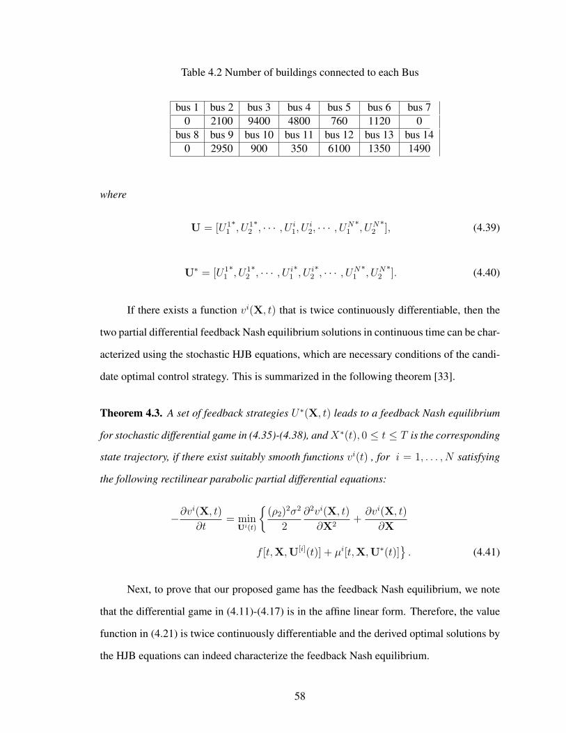
Table 4.2 Number of buildings connected to each Bus
bus 1 bus 2 bus 3 bus 4 bus 5 bus 6 bus 70 2100 9400 4800 760 1120 0
bus 8 bus 9 bus 10 bus 11 bus 12 bus 13 bus 140 2950 900 350 6100 1350 1490
where
U = [U11∗, U1
2∗, · · · , U i
1, Ui2, · · · , UN
1
∗, UN
2
∗], (4.39)
U∗ = [U11∗, U1
2∗, · · · , U i
1
∗, U i
2
∗, · · · , UN
1
∗, UN
2
∗]. (4.40)
If there exists a function vi(X, t) that is twice continuously differentiable, then the
two partial differential feedback Nash equilibrium solutions in continuous time can be char-
acterized using the stochastic HJB equations, which are necessary conditions of the candi-
date optimal control strategy. This is summarized in the following theorem [33].
Theorem 4.3. A set of feedback strategies U∗(X, t) leads to a feedback Nash equilibrium
for stochastic differential game in (4.35)-(4.38), and X∗(t), 0 ≤ t ≤ T is the corresponding
state trajectory, if there exist suitably smooth functions vi(t) , for i = 1, . . . , N satisfying
the following rectilinear parabolic partial differential equations:
−∂vi(X, t)
∂t= min
Ui(t)
{(ρ2)
2σ2
2
∂2vi(X, t)
∂X2+
∂vi(X, t)
∂X
f [t,X,U[i](t)] + µi[t,X,U∗(t)]}. (4.41)
Next, to prove that our proposed game has the feedback Nash equilibrium, we note
that the differential game in (4.11)-(4.17) is in the affine linear form. Therefore, the value
function in (4.21) is twice continuously differentiable and the derived optimal solutions by
the HJB equations can indeed characterize the feedback Nash equilibrium.
58

Figure 4.2 The fourteen bus system studied in simulations.
4.4 Simulation Results
In this section, we numerically investigate the performance of the proposed stochastic
differential game to confirm and complement the results presented in the previous sections.
Consider the IEEE 14-bus test system in Figure 4.2, where the load at each bus is the sum-
mation of several homogeneous smart building load at that bus. The number of buildings
that are connected to each bus is shown in Table 4.2. The bus and the line parameters are
set according to the model in [78]. According to [79], the lead-acid batteries which are
suitable for energy-smart buildings are generally 85-95 % efficient. Therefore, for simula-
tion purposes the value for the leakage rate of the batteries is considered to be β = 0.05.
The value for ϵ as the factor of inertia of the building is a function of the time constant of
the building which can be defined as the energy stored per unit area in the construction per
unit change in heat flux. Finally, the overall thermal conductivity is calculated based on
the real data for a typical building in Texas provided by [80] as 0.5. The price factors in
equation (4.2) are set as pc = 0.055$KWh and α = 1.
To study how the proposed demand response method affects electricity scheduling
at the buildings level, we compare the performance of our algorithm with a more realistic
day-ahead pricing scenario. In the day ahead pricing scenario, the 24-hour price profile
59

2 4 6 8 10 12 14 16 18 20 22 240.056
0.057
0.058
0.059
0.06
0.061
0.062
0.063
Time (Hour)
Pric
e ($
/kW
h)
Day−Ahead PricingReal Time Pricing
Figure 4.3 Daily price for two pricing scenarios.
is assumed to be known to the ECS from day before and taken from real data [80] of
one day consumption as shown in Figure 4.3. We also show the real-time pricing in the
same figure. For simplicity, we focus on one building at bus number 2 as an example.
The outdoor temperature, the mean of wind turbine output, and the uncontrollable load are
depicted in Figure 4.4(a), Figure 4.4(b) and Figure 4.4(c), respectively [80].
In Figures 4.5(a) and 4.5(b), the daily states of the considered building for the men-
tioned three methods are depicted. For all three scenarios, as price tends to increase, the
battery tends to discharge in order to cover a portion of the building power consumption.
Furthermore, the indoor temperature tends to increase due to lowering the air conditioner’s
load during peak hours. We can also see that, for all scenarios, the variations of both battery
level and the indoor temperature are correlated to the changes in price values. Here, the
average usage from the battery reduces by around 10% for real-time pricing in peak hours
(18-20) compared to the day-ahead pricing case.
Next, we compare our proposed joint real-time pricing at upper level and demand
response at lower level, with the two other design scenarios. The corresponding daily load
profiles are shown in 4.6. For both day-ahead and real-time pricing techniques, the peak
60

Table 4.3 Average daily market profit vs. building’s cost
Real-time Pricing Day-ahead PricingMarket Profit ($) 48609 48741
Average Building’s Cost ($) 229 241
load is reduced at around 8:00 PM. However, the use of the proposed real-time pricing
technique yields a more flat load shape compared to other methods.
Figure 4.7 studies how the PAR in aggregate load varies as the mean of the daily
outdoor temperature increases for three pricing scenarios. As it is shown in Figure 4.6
compared to the other technique, the proposed real pricing technique makes the load curve
more flat. Therefore, the PAR of associated load curve is also have the least value. Due
to the fact under high temperature, users tend to let AC unit stay on for longer time, e.g.
even at night when the load is low. Consequently, the PAR decreases as the temperature
increases, roughly in form of a linear function.
The mean daily cost of the considered building versus the mean daily outdoor tem-
perature are shown in Figure 4.8. We can see that the real-time pricing combined with the
proposed stochastic differential game can reduce the daily cost. The price value under the
real-time pricing has higher gradient since all building users increase their power consump-
tion in the case of a high temperature, which results in a higher price. Moreover, when the
temperature is high, the HVAC units are needed to stay functioning in order to keep the
indoor temperature in the comfort range of users. Therefore, there is no major difference
among different algorithms in this case as Figure 4.8 suggests.
The average daily market profit versus the building’s costs are compared in Table 4.3.
The profit is calculated as the total market revenue reduced from the total generation cost.
The generation cost per hour is calculated according to [81] as 0.00128D2 + 6.48D+ 459,
where D is the total demand. As the table suggests, by deploying the real-time pricing
technique compared to the day-ahead pricing, the buildings can reduce their cost approxi-
mately 5% while the market will face 0.27 % reduction in the daily profit, which is quite
61
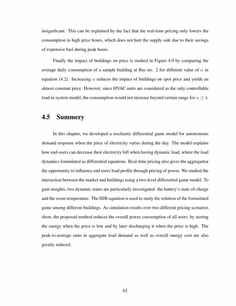
insignificant. This can be explained by the fact that the real-time pricing only lowers the
consumption in high price hours, which does not hurt the supply side due to their savings
of expensive fuel during peak hours.
Finally the impact of buildings on price is studied in Figure 4.9 by comparing the
average daily consumption of a sample building at Bus no. 2 for different value of α in
equation (4.2). Increasing α reduces the impact of buildings on spot price and yields an
almost constant price. However, since HVAC units are considered as the only controllable
load in system model, the consumption would not increase beyond certain range for α ≥ 4.
4.5 Summery
In this chapter, we developed a stochastic differential game model for autonomous
demand response when the price of electricity varies during the day. The model explains
how end-users can decrease their electricity bill when having dynamic load, where the load
dynamics formulated as differential equations. Real-time pricing also gives the aggregartor
the opportunity to influence end users load profile through pricing of power. We studied the
interaction between the market and buildings using a two-level differential game model. To
gain insights, two dynamic states are particularly investigated: the battery’s state-of-charge
and the room temperature. The HJB equation is used to study the solution of the formulated
game among different buildings. As simulation results over two different pricing scenarios
show, the proposed method reduces the overall power consumption of all users, by storing
the energy when the price is low and by later discharging it when the price is high. The
peak-to-average ratio in aggregate load demand as well as overall energy cost are also
greatly reduced.
62

2 4 6 8 10 12 14 16 18 20 22 2476
78
80
82
84
86
88
90
92
Time (Hour)
Out
door
Tem
erat
ure
(Fah
renh
eit)
(a) Outdoor Temperature
5 10 15 201
1.5
2
2.5
3
3.5
4
4.5
5
Time (Hour)
Win
d T
urbi
ne O
utpu
t (K
Wat
t)
(b) Predicted Ouptput of Wind Turbine
5 10 15 20
2.55
2.6
2.65
2.7
2.75
Time (Hour)
Bui
ldin
g U
ncon
trol
labl
e Lo
ad (
KW
Att)
(c) Uncontrollable Load
Figure 4.4 Region characteristics at Bus 2.
63
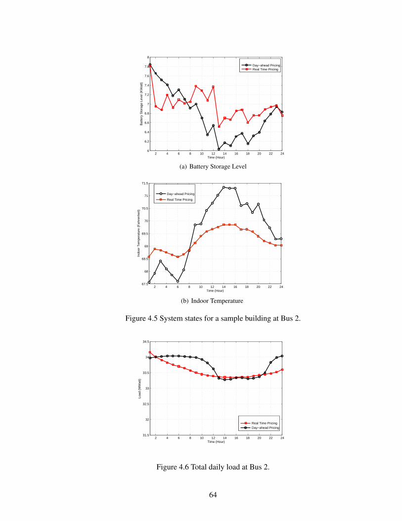
2 4 6 8 10 12 14 16 18 20 22 246
6.2
6.4
6.6
6.8
7
7.2
7.4
7.6
7.8
8
Time (Hour)
Bat
tery
Sto
rage
Lev
el (
KW
att)
Day−ahead PricingReal Time Pricing
(a) Battery Storage Level
2 4 6 8 10 12 14 16 18 20 22 2467.5
68
68.5
69
69.5
70
70.5
71
71.5
Time (Hour)
Indo
or T
empe
ratu
re (
Fah
renh
eit)
Day−ahead Pricing
Real Time Pricing
(b) Indoor Temperature
Figure 4.5 System states for a sample building at Bus 2.
2 4 6 8 10 12 14 16 18 20 22 2431.5
32
32.5
33
33.5
34
34.5
Time (Hour)
Load
(M
Wat
t)
Real Time PricingDay−ahead Pricing
Figure 4.6 Total daily load at Bus 2.
64
80 85 90 95 1001
1.01
1.02
1.03
1.04
1.05
1.06
Outdoor Temperature (Fahrenheit)
Ave
rage
PA
R
Day−Ahead PricingReal Time Pricing
Figure 4.7 Comparison of load PAR for two pricing scenarios.
80 85 90 95 100180
200
220
240
260
280
300
320
Outdoor Temperature (Farenheit)
Ele
ctric
ity B
ill (
$)
Day−Ahead Pricing
Real Time Pricing
Figure 4.8 Daily cost vs. outdoor temperature for two pricing scenarios.
65

1 2 3 4 50
5
10
15
20
25
30
35
α
Ave
rage
Dai
ly P
ower
Con
sum
ptio
n of
a B
uild
ing
(kw
att)
Figure 4.9 Impact of buildings power consumption on price
66

Chapter 5
Distributed Control of HVAC Systems in SmartBuildings
5.1 Introduction
Buildings consume almost 70% of the total electricity generated in the US [83, 84].
One of the major energy-consuming systems of a building is the heating, ventilation and
air conditioning (HVAC) system. More precisely, an HVAC system might exhaust more
than 65% of the total electrical energy consumed by a building [85–87]. The high energy
consumption of HVAC systems raises energy costs as well as environmental concerns.
Therefore, a desirable capability of future “smart buildings” is energy reduction via fine-
grained control of HVAC systems. For instance, an HVAC system can be conceived as an
autonomous system that adjusts the indoor temperature of different locations in the building
based on the occupancy [88].
A growing body of research suggests that efficient control of HVAC systems might
significantly increase the energy efficiency of future smart-buildings. For instance, in
[89], the authors explored the problem of computing optimal control strategies for time-
scheduled operation taking into consideration building operation schedules, e.g., night-
setback, start-up and occupied modes, as well as a predicted weather profile. In [90], dy-
namic and real-time simulation models are developed to study the thermal, hydraulic, me-
chanical, environmental and energy performance of smart buildings. In [91], the authors
presented a simulation tool, “QUICK Control”, to predict the effect of changing control
strategies on indoor comfort and energy consumption.
For occupancy-based control of HVAC systems, a fundamental requirement is a sen-
sor network to capture the occupancy changes in real time. In [92], the authors proposed
67

several control strategies based on real time occupancy monitoring and occupancy predic-
tions.
In this paper, tools from game theory and multi-agent learning are used to design a
cost-efficient distributed control for HVAC systems. This work takes into consideration the
electricity cost and predetermined ranges of desirable temperatures during certain periods
for all locations in the building that are subject to temperature control. The main game-
theoretic tool of this analysis is the notion of a satisfaction equilibrium (SE) [24]. Basically,
an SE is an equilibrium concept in which players do not seek any benefit maximization but
only the satisfaction of their own individual constraints. This equilibrium is thoroughly
studied in the context of the distributed control of HVAC systems. More importantly, a
simple algorithm based on the notion of trial-and-error learning [94] that is capable of
achieving an SE is also presented.
The rest of this paper is organized as follows. Section 5.2 introduces the system
model. Section 5.3 describes two games, one in the satisfaction form and another one in
the normal form, to model the problem of distributed control of HVAC systems. Therein, a
fully distributed learning algorithm is also provided to achieve the equilibria of the corre-
sponding games. Section 5.5 presents some simulation results, and Section 5.6 concludes
this work.
5.2 System Model
Consider a smart-building with n zones subject to temperature control. Each zone is
managed by an HVAC system that is fully independent of all the other HVAC units in the
building. The goal is to reduce the electricity cost by dynamically adjusting the operation
of the HVAC units such that two main constraints are satisfied: (i) The temperature of
a given room i, with i ∈ {1, . . . , n} must be kept within a desirable range for certain
predetermined periods; and (ii) The total power load dedicated for heating, ventilation and
68
air conditioning must not exceed a predetermined threshold.
Consider that temperature is controlled with a granularity of 1 hour. At the beginning
of the day, HVAC unit i chooses its own daily power consumption vector, denoted by,
Li = (li(1), ..., li(t), ..., li(24)), where li(t) denotes the power consumed by HVAC unit i
at hour t. Each HVAC unit chooses its vector Li from a finite set of vectors denoted by Li.
The daily power consumption vector is selected in order to minimize the daily electricity
cost
Φ(L,P) =n∑
i=1
24∑t=1
µi(li(t), p(t)), (5.1)
where L = (L1, . . . ,Ln) ∈ L1 × . . . × Ln, P = (p(1), . . . , p(24)) ∈ R24 , with p(t) the
hourly market price per energy unit. Note that the vector P is assumed to be known by
each HVAC unit at the beginning of the day. The function µi : Li × R → R models
the operation cost of HVAC i with power load li(t) and price pi(t). One example of the
function µi is presented in [95]. Therein, the function µi is defined as follows:
µi(li(t), p(t)) = c1p(t)li(t)2 + c2p(t)li(t) + c3, (5.2)
where c1, c2 and c3 are constant parameters that are determined based on experimental data.
One of the advantages of a quadratic model for the operation cost of an HVAC unit is that
it is more realistic and flexible than other models, e.g., the translog cost model [96].
The total power load allocated for the HVAC system satisfies the following constraint
at each 1-hour period t of the day:
∀t∈ {1, . . . , 24},n∑
i=1
li(t) ≤ Lr, (5.3)
where the threshold value Lr is imposed by the characteristics of the power distribution
feeder/bus of the building. This threshold is assumed to remain the same at each period t.
69
The temperature Ti(t) of zone i during period t must fall within the interval [T ti, T
ti ].
Note that this control is enforced only during certain periods. Hence, the set Ii denotes the
periods over which this rule is enforced, i.e.,
∀t ∈ Ii, T ti ≤ Ti(t) ≤ T t
i . (5.4)
For all the other periods t ∈ {1, . . . , 24} \ Ii no temperature control is performed. The
indoor temperature is predicted up to 24 hours in advance using a simple exponential decay
model proposed by [73]. That is,
Ti(t+ 1) = ϵTi(t) + (1− ϵ)(TOD(t)− γKli(t)), (5.5)
where ϵ is the thermal time constant of the building; γ is a factor capturing the efficiency of
the air conditioning unit to cool the air inside the building ; TOD is the outside temperature
which is predicted a day ahead; and K is a conversion factor that is proportional to the
performance coefficient of the HVAC unit divided by the total thermal mass. The HVAC
unit uses power li(t) to control the temperature of zone i during period t. In this model, our
focus is only on the cooling scenario. The results for a heating scenario can also be easily
obtained by changing the sign of −γKli(t).
Equation (5.5) explains how the constraint (5.4) relates to the power consumed by
the HVAC unit. The HVAC control units should select their consumption amounts in a way
that the indoor temperature obtained from (5.5) falls within the comfort interval (5.4) and
minimize the total cost in (5.1). That is, the vector L = (L1, . . . ,Ln) must be chosen such
that
minL∈L1×...×Ln
n∑i=1
24∑t=1
µi(li(t), p(t)) (5.6)
s.t.n∑
i=1
li(t) ≤ Lr, ∀t ∈ {1, . . . , 24} and
T ti ≤ Ti(t) ≤ T t
i , ∀t ∈ Ii.
70

The above problem can be solved at the beginning of the day such that the vector Li =
(li(1), ..., li(t), ..., li(24)) is entirely calculated by HVAC i only once per day; or at each
period t, the HVAC determines its individual load li(t+1). Both alternatives are studied in
Section 5.4.
5.3 Game Formulation
The distributed control problem of the HVAC system described above can be mod-
eled via two games formulations: a game in normal form [97] and a game in satisfaction
form [24].
5.3.1 Game in Normal Form
Consider the game in normal form
G = (N ,L, {ξi}{i∈N}). (5.7)
The set N = {1, . . . , n} represents set of players. HVAC i is represented by player i. The
set of actions of player i is the set of daily power consumption vectors Li. Hence, the set
of actions of the game is L = L1 ×L2 × . . .Ln. The payoff function ξi : L×R24 → R of
player i is defined by
ξi(L,P) =1
β + 1
(1−
∑24t=1 µi(li(t), p(t))
24µmax
+ β1{Li∈fi(L−i)}
), (5.8)
where β is a design parameter, µi is defined in (5.2) and µmax is the maximum cost user
i can experience. The correspondence fi : L1 × . . . × Li−1 × Li+1 × . . . × Ln → 2Li is
defined as follows:
fi(L−i) ={
Li ∈ Li : ∀t ∈ {1, ..., 24} (5.9)
n∑i=1
li(t) ≤ Lr and T ti ≤ Ti(t) ≤ T t
i
}.
71

The payoff function in (5.8) captures the tradeoff between satisfying the individual con-
straints of player i and minimizing the individual consumption cost. Note that increasing
the value of β leads to the player focusing on in the satisfaction of its individual constraints.
Alternatively, reducing the value of β leads the player to focus more on the reduction of
the individual operating cost. This utility function was first proposed in [26] for the case of
decentralized radio resource allocation in wireless networks.
An interesting outcome of the game G is a Nash Equilibrium (NE), which is defined
as follows:
Definition 1. An action profile L∗ ∈ L of the game (5.7) is an NE if ∀i ∈ N and ∀L′
i ∈ Li,
ξi(L∗i ,L∗
−i,P) ≥ ξi(L′
i,L∗−i,P). (5.10)
The interest in the NE stems from the fact that at such a state, none of the players can
improve its payoff by unilaterally changing its action.
5.3.2 Game in Satisfaction Form
Consider the game in satisfaction form G = (N ,L, {fi}{i∈N}). In the game G, a
player is said to be satisfied if it plays an action that satisfies its individual constraints.
More importantly, once a player satisfies its individual constraints, it has no interest in
changing its action, and thus, an equilibrium is observed when all players are simultane-
ously satisfied. This equilibrium is often referred to as the satisfaction equilibrium [24].
Definition 2. An action profile L+ ∈ L is a satisfaction equilibrium for the game G =
(N ,L, {fi}{i∈N}) if
∀i ∈ N , L+i ∈ fi(L+
−i). (5.11)
The interest in the SE stems from the fact that at such a state, all players satisfy their
individual constraints. However, no optimality can be claimed on the choices of the players
with respect to the cost in (5.1).
72
5.4 The distributed learning algorithm
In this section, a learning algorithm based on a trial-and-error dynamics is proposed
to distributively achieve an SE and/or NE.
5.4.1 Trial and Error Learning Algorithm
Player i locally implements a state machine. At iteration s, the state of player i is
defined by the triplet
Zi(s) = {mi(s), Li(s), ξi(s)}, (5.12)
where mi(s) represents the “mood” of player i, that is, the way it reacts to the observation
of the instantaneous observation ξi(s) of ξi(L(s),P), with ξi defined in (5.8) and L(s) is
the action played at iteration s. Li(s) ∈ L and ξi(s) ∈ [0; 1] represent a benchmark action
and a benchmark payoff, respectively. There are two possible moods: content (C) and
discontent (D); and thus, mi(s) ∈ {C,D}.
If at iteration s player i is content, it chooses action Li following the probability
distribution
πi,Li=
{ϵc
|Li|−1, if Li ≥ Li,
1− ϵc, if Li = Li,
where, πi,Li= Pr(Li(s) = Li), c > n is a constant and ϵ > 0 is an experimentation rate.
In the following, we use the notation X ⇐ Y to indicate that variable X takes the value
of variable Y . If player i uses its bench-marked action at iteration s, i.e, Li(s) = Li, and
ξi(s+ 1) = ξi(s) then the state Zi(s) remains the same. Otherwise, it adopts a new bench-
marked action and a new benchmark payoff: Li(s + 1) ⇐ Li(s), ξi(s + 1) ⇐ ξi(s). The
mood of player i is updated as follows: with probability ϵ(1−ξi(s)) it sets its mood to content
mi(s+1) ⇐ C, and with probability 1−α(1−ξi(s)), it sets it to discontent mi(s+1) ⇐ D.
73

5.4.2 Properties
An essential condition for the mentioned learning algorithm to achieve a stochasti-
cally stable state is the interdependence property defined as follows [94].
Definition 3. (Interdependent game) An n-person game G on the finite action set L is inter-
dependent if for every non-empty subset J ⊂ N and every action profile L = (LJ ,L−J ) ∈
L such that LJ is the action profile of all users in J , there exists a player i ∈ N such that
∃L′
J = LJ : ξi(L′
J ,L−J ) = ξi(LJ ,L−J ). (5.13)
In other words, the interdependence condition states that it is not possible to divide
the players into two separate subsets that do not interact with each other.
In the following, we assume that game G is interdependent. This is a reasonable as-
sumption, since the power consumption choices of all players affects the set of conditions
in (5.3) that all other players should satisfy. The following theorem states that the play-
ers’ actions at the stochastically stable state of the learning algorithm maximize the social
welfare of all players [94].
Theorem 5.1. Under the dynamics defined by the mentioned learning algorithm, a state
Z = (m,L, ξ), is stochastically stable if and only if the following conditions are satisfied:
• The action profile L maximizes the social welfare function W : L × R24 → R,
defined as follows:
W (L,P) =∑i∈N
ξi(L,P). (5.14)
• The mood of each player is content.
The next theorem states that by selecting β > n, the stochastically stable state of the
dynamics described above is such that the largest set of players is satisfied.
74
Theorem 5.2. Let each player in the game G implement the learning algorithm described
above with utility function ξi and β > n. Then, the action profile with the highest social
welfare satisfies the highest number of players.
Proof. It is sufficient to show that if L∗ is an action profile that satisfies k∗ players and L′
an action profile that satisfies k′ players, and k∗ > k
′ , then W (L∗) > W (L′). We have
W (L) as follows:
W (L)∑i∈N
1
β + 1
(1−
∑24t=1 µi(li(t), p(t))
24µmax
+ β1{Li∈fi(L−i)}
), (5.15)
and we also have:
0 ≤∑i∈N
(1−
∑24t=1 µi(li(t), p(t))
24µmax
)≤ n. (5.16)
Using the inequality (5.16), and the assumption that L∗ is an action profile which satisfies
k∗ players, we can write βk∗
1+β≤ W (L∗) ≤ n+βk∗
1+β. Similarly using (5.16) and the assumption
that L′is an action profile which satisfies k′ players, we can write βk
′
1+β≤ W (L′
) ≤ n+βk′
1+β.
Since k∗, k′ ∈ N, we can write the assumption k′< k∗ as k
′ ≤ k∗ − 1, which implies
W (L′) ≤ n+βk
′−β1+β
. Using the assumption that β > n, we can write n+βk′−β
1+β< βk
′
1+β.
Following the set of inequalities, we can state W (L′) < βk
′
1+β≤ W (L∗), which proves
W (L∗) > W (L′).
5.4.3 Online Scheduling
The day-ahead scheduling method as it is described in Section 5.2 can achieve a sat-
isfaction equilibrium using the distributed learning method in the convergence as is proven
in Theorem 2. Due to the constant change of the outdoor temperature and market electricity
price, it is more practical that scheduling of HVAC units be performed on a hourly basis
75

instead of a day-ahead one. In this section we explain the details of the hourly scheduling
method.
For the hourly scheduling method, each HVAC unit chooses its hourly consumption
li from a finite set denoted by L′i. The constrained electricity cost optimization of each
zone as defined in (5.6) can be rewritten as follows at time interval t:
minL∈L′
i×...×L′n
n∑i=1
µi(li(t), p(t)) (5.17)
s.t.n∑
i=1
li(t) ≤ Lr,
T ti ≤ Ti(t) ≤ T t
i ,
where L(t) = [l1(t), . . . , ln(t)].
The game definition for the normal and satisfaction forms change accordingly as
follows.
5.4.3.1 Game in Normal Form
The game in normal form is represented by the triplet, G = (N ,L′, {ξi}{i∈N}). Here,
N = {1, . . . , n} represents the set of players that are HVAC control units of n zones. The
action of player i is its hourly power consumption, li(t), and each player i has a finite set
of actions, L′i. The set of actions of the game is the joint set of players actions, L′
=
L′1 × L′
2 × . . .L′n. We introduce the payoff function of player i, ξ′
i : L′ → R defined by
ξ′
i(li(t),L−i(t)) =1
β + 1
(1− µi(li(t), p(t))
µmax
+ β1{li(t)∈f ′i(L−i(t))}
), (5.18)
where we define f ′i : L1 × . . .× Li−1 × Li+1 × . . .× Ln → 2Li as follows:
f ′i(L−i) =
{li ∈ L′
i :n∑
i=1
li ≤ Lr, Tti ≤ Ti(t) ≤ T t
i
}.
76
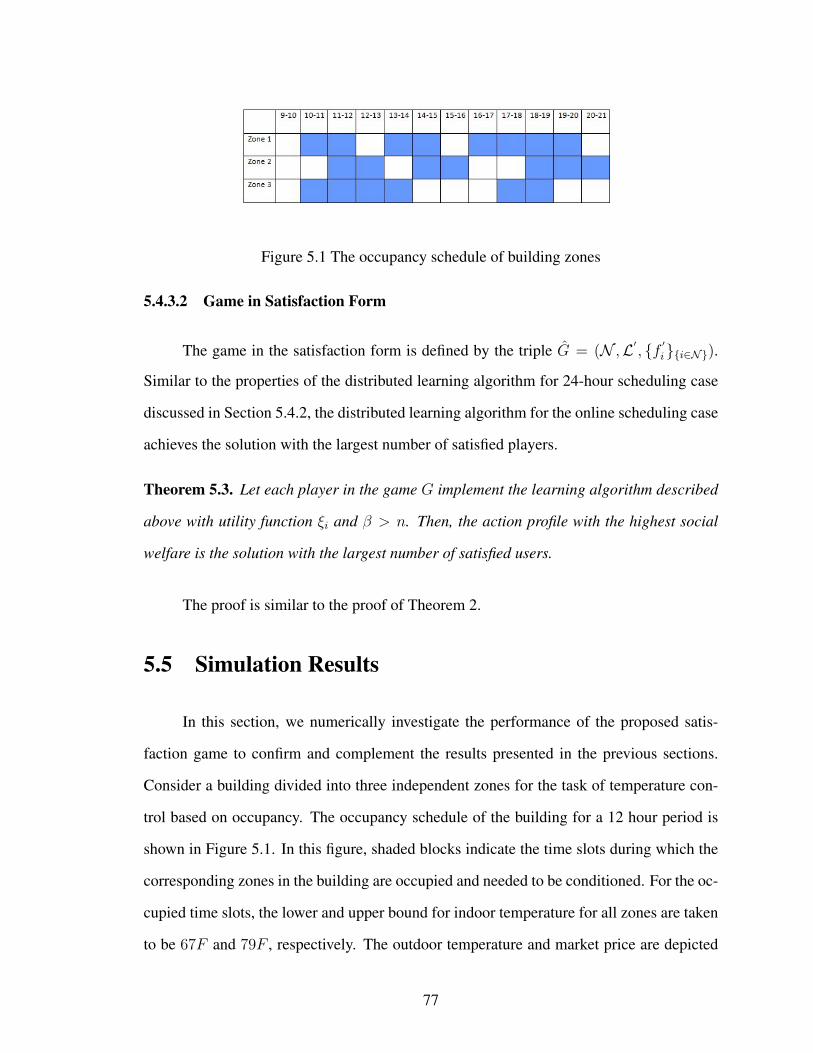
Figure 5.1 The occupancy schedule of building zones
5.4.3.2 Game in Satisfaction Form
The game in the satisfaction form is defined by the triple G = (N ,L′, {f ′
i}{i∈N}).
Similar to the properties of the distributed learning algorithm for 24-hour scheduling case
discussed in Section 5.4.2, the distributed learning algorithm for the online scheduling case
achieves the solution with the largest number of satisfied players.
Theorem 5.3. Let each player in the game G implement the learning algorithm described
above with utility function ξi and β > n. Then, the action profile with the highest social
welfare is the solution with the largest number of satisfied users.
The proof is similar to the proof of Theorem 2.
5.5 Simulation Results
In this section, we numerically investigate the performance of the proposed satis-
faction game to confirm and complement the results presented in the previous sections.
Consider a building divided into three independent zones for the task of temperature con-
trol based on occupancy. The occupancy schedule of the building for a 12 hour period is
shown in Figure 5.1. In this figure, shaded blocks indicate the time slots during which the
corresponding zones in the building are occupied and needed to be conditioned. For the oc-
cupied time slots, the lower and upper bound for indoor temperature for all zones are taken
to be 67F and 79F , respectively. The outdoor temperature and market price are depicted
77

10 12 14 16 18 2083
84
85
86
87
88
89
90
91
92
Time (Hour)
Out
door
Tem
pera
ture
(F
ahre
nhei
t)
(a) Outdoor Temperature
10 12 14 16 18 200.0561
0.0562
0.0563
0.0564
0.0565
0.0566
0.0567
0.0568
Time (Hour)
Pric
e ($
/KW
h)
(b) Electricity Price
Figure 5.2 Characteristics of the building
in Figure 5.2(a) and Figure 5.2(b), respectively according to data in [80].
Other simulation parameters are set as ϵ = 0.7, λ = 0.9, K = 15, c1 = c2 = c3 = 1,
B = 100 and Lr=1.5 KW . The energy consumption of the HVAC units is assumed to
be chosen from the set {0, 0.2, 0.4} for both games. First, we compare the payoff of our
proposed game in the satisfaction form with its payoff in the normal form and the payoff
of the maximum social welfare solution as shown in Figure 5.3. The learning algorithm
parameter is set at α = 0.05 and the number of iteration is 10000. The proposed learning
algorithm is able to meet the optimal solution for most of the time (stochastically stable
state). For the game in normal form, players can achieve NE after a few iterations, and the
payoff of players is considerably lower than the maximum spacial welfare.
78

0 1000 2000 3000 4000 5000 6000 7000 8000 9000 100000
1
2
3
4
5
6
7
8
9x 10
−3
Number of Iterations
Pay
off
Maximum Social WelfareSENE
Figure 5.3 Payoff versus the number of iterations
Figure 5.4 studies the effect of exploration rate (α) on the convergence of the game’s
payoff in satisfaction form to the maximum social welfare. As the figure shows, by de-
creasing the exploration rate from 0.05 to 0.01, the players tend to stick to their choices.
Therefore, the learning algorithm might temporary stabilize at a non-optimal state. On the
the other hand by increasing the exploration rate from 0.05 to 0.09, the payoff decreases
again. This can be explained since for higher exploration rates, players choose their ac-
tions more dynamically, and consequently the algorithm might not be stable even if it has
converged to the maximum social welfare.
Next we compare the average conditioned indoor temperature during the scheduled
time slots for zone 1 versus the achieved payoff for the four cases of day-ahead SE, day-
ahead NE, real-time SE and real-time NE in Figure 5.5. Note that the payoff function for
12-hour cases are different from that for the real-time cases. However, the payoff achieved
by the game in satisfaction form is higher than that of the game in normal form at the cost
of higher average indoor temperature.
Finally, Figure 5.6 shows by increasing the number of granularity levels of the power
consumed by HVAC units, the payoff increases and finally archives the maximum social
79

0 0.01 0.02 0.03 0.04 0.05 0.06 0.07 0.08 0.09 0.150
55
60
65
70
75
80
85
90
Exploration Rate (α)
Per
cent
age
of C
onve
rage
nce
to T
he O
ptim
al S
olut
ion
Figure 5.4 Satisfaction game convergence versus the exploration rate
welfare solution with the continuous action set. Having 9 power levels, the SE has a similar
payoff to the maximum social welfare solution, and significantly better payoff compared to
the NE payoff.
5.6 Summary
HVAC control units of multiple zones in a smart building to achieve SE. In particular,
the proposed learning algorithm is able to control the power consumption levels of HVAC
units in order to guarantee that the largest number of zones have stochastically stable in-
door temperatures which are falling within the predetermined comfort range of users, while
incurring the minimum electricity cost. To implement the proposed game in the satisfac-
tion form and the proposed learning algorithm, the HVAC unit of each zone only requires
little information from other zones. Simulation results demonstrate the properties of the
proposed game and show how HVAC control units can reduce the building electricity cost
effectively while satisfying the constraints.
80

73 73.5 74 74.55
5.5
6
6.5
7
7.5
8
8.5
9
9.5
10x 10
−3
Average Indoor Temeparture (Fahrenheit)
Pay
off
Real−TimeSE
SE
Real−Time NE
NE
Figure 5.5 The payoff versus the average indoor temperature
3 4 5 6 7 8 95
5.5
6
6.5
7
7.5
8
8.5
9
9.5
x 10−3
Number of Power Levels
Pay
off
SEMaximum Social WelfareNE
Figure 5.6 Payoff versus the number of power levels
81

Chapter 6
Conclusion and Future Work
6.1 Conclusion
The smart grid is envisioned to be a large-scale cyber-physical system composed of
intelligent nodes that can operate, communicate, and interact autonomously in order to ef-
ficiently deliver power to their consumers. The heterogeneous and decentralized nature of
the smart grid motivates adoption of game theory for overcoming various design, control,
and implementation challenges. In this dissertation, we proposed game theatrical frame-
works for distributed dynamic control application in smart grid systems. We summarize
the research that has been completed for each of these frameworks in this chapter.
First we studied the problem of optimal distributed generation and storage for ther-
mal and pumped-storage power plants in a smart grid network. We proposed a stochastic
differential game approach to model their competition and derived the optimal strategies
for both players if the other’s action is fixed using HJB equations. We showed that there
exists the feedback Nash equilibrium strategies for the proposed game. Simulation results
demonstrate the properties of the proposed game and suggest how the two types of power
plants need to adjust their generating and storage decision variables to maximize their rev-
enues. It is demonstrated that the proposed framework and games can reduce the peak to
average ratio and total energy generation for the thermal plant, which helps power plant
operation and reduces CO2 emission.
Next, we considered smart buildings equipped with renewable resources generators,
local energy storage and controllable HVAC units, in which users are able to respond to
real-time grid conditions like electricity prices and weather conditions in order to minimize
their cost. We modeled the strategic interactions between such energy-smart buildings and
a Nash-Cournot electricity market using a two-level stochastic differential game frame-
82
work. At the upper level, the market offers a vector of hourly prices to end users. At the
lower level, the energy-smart buildings as the lower level participate in demand response
by managing controllable dynamic load in response to hourly prices set by the market.
Specifically, two dynamic states in energy-smart buildings are investigated: the battery’s
state-of-charge and the room temperature. The solution of the formulated game among
different buildings is derived by HJB equations. As simulation results show, the proposed
method reduces the overall power consumption of all users, by storing the energy when the
price is low and by later discharging it when the price is high. The peak-to-average ratio of
aggregate load demand as well as overall energy cost is also greatly reduced.
Finally, we focused distributed control of HVAC systems as major consumption units
in buildings. The problem of electricity cost efficient scheduling of HVAC units while sat-
isfying predetermined ranges of desirable temperatures during certain periods for multiple
zones in the building that are subject to temperature control is taken into consideration.
The game-theoretic tool used to analysis this problem is satisfaction equilibrium, in which
players do not seek any benefit maximization but only the satisfaction of their own indi-
vidual constraints. The notion of satisfaction game enables players to make stochastically
stable decisions with limited information from the rest of players. To achieve satisfaction
equilibrium, a trial-and-error learning is proposed. We showed that this algorithm reaches
stochastically stable control decisions that are equilibria and maximizers of the global wel-
fare of the corresponding game. The propertied of proposed game and learning algorithms
are studied for both day-ahead and real-time cases through simulation results.
6.2 Future Work
This section includes the overview of future research and possible progressions in
the studied problems in this dissertation on distritbuted dynamic control schemes for smart
grid networks. We introduce the following topics that can be chosen for further advanced
83

research.
• Design of multi-stage game-theoric frameworks for integration of distributed gen-
eration units to smart grids’ electricity markets in order to achieve optimal trading
prices among competing distributed generation entities as well as optimal generation
or storage decisions.
• Incorporation of mean field games [98, 99] for distributed control applications with
extremely large number of players such as large number of buildings, PHEV vehicles,
and so on in order to avoid the high volume overhead of feedback information which
enforce timing delays and data storage costs to the grid. In contrast to N-player
games, where each player follows the evolution of the state of the game and the
actions taken by all other players in order to maximize a given individual benefit, in
the mean field game formulation, every players action is driven by the collective (or
mean) behavior of all players and not by the individual actions of each other player.
As a main consequence, it is possible in these games to follow the state trajectory of
all players at once and to capture the behavior of the players depending only on their
initial state and the joint distribution.
• Sensor-driven analysis to obtain full picture of almost every aspect of the buildings
states and dynamics for more efficient buildings energy management systems. For
example, using infrared sensors to determine whether a space is occupied or not, how
much daylight there is, whether the lights are on and what level of lighting they pro-
vide would enables design of more efficient lighting control systems. Integrated data
from sensors in electricity and water meters, lighting, HVAC systems, geothermal
pumps [100] and other subsystems will provide immediate insight into the overall
state of the buildings dynamic systems, as well as design of energy efficient dis-
tributed controls.
84

Bibliography
[1] Office of electricity delivery and energy reliability, “Smart grid”, August 2009,
http://www.oe.energy.gov/smartgrid.htm.
[2] P. E. Marken, J. J. Marczewski, R. D’Aquila, P. Hassink, J. H. Roedel, and R. L. Bodo,
“VFT - a smart transmission technology that is compatible with the existing and future
grid,” in proceedings of IEEE/PES Power Systems Conference and Exposition, PSCE
’09., March 2009.
[3] A. Ipakchi and F. Albuyeh, “Grid of the future,” IEEE Power and Energy Magazine,
vol.7, no.2, pp.52–62, March 2009.
[4] H. Farhangi, “The path of the smart grid,” IEEE Power Energy Magazine, vol. 8, no.
1, pp. 1828, Feb. 2010.
[5] F. Li, W. Qiao, H. Sun, H. Wan, J. Wang, Y. Xia, Z. Xu, and P. Zhang, “Smart trans-
mission grid: Vision and framework,” IEEE Transactions on Smart Grid, vol. 1, no.
2, 2010.
[6] X. Fang, S. Misra, G. Xue, and D. Yang, “Smart grid - the new and improved power
grid: A survey,” IEEE Commun. Surveys Tutorials, 2012.
[7] C. Lo and N. Ansari, “The progressive smart grid system from both power and com-
munications aspects,” IEEE Commun. Surveys Tutorials, 2012.
[8] P. Zhang, F. Li, and N. Bhatt, “Next generation monitoring, analysis and control for
the future smart control center,” IEEE Trans. Smart Grid, vol. 1, no. 2, Sep. 2010.
[9] J. R. Roncero, “Integration is key to smart grid management,” in Proc. IET-CIRED
Seminar SmartGrids Distribution, pp. 14, June 2008.
[10] PJM Brochure, “Bringing the Smart Grid Idea Home,” 2007.
85

[11] B. Heile, “Smart grids for green communications,” IEEE Wireless Communications,
vol. 17, no. 3, pp. 46, Jun. 2010.
[12] S. Ramchurn, P. Vytelingum, A. Rogers, and N. R. Jennings, “Agent based homeo-
static control for green energy in the smart grid,” ACM Transactions on Intelligent
Systems and Technologies, vol. 2, no. 4, Jul. 2011.
[13] S. Lukovic, I. Kaitovic, M. Mura, and U. Bondi, “Virtual power plant as a bridge
between distributed energy resources and smart grid,” in proceedings of 43rd Hawaii
International Conference on System Sciences (HICSS), Switzerland, January 2010.
[14] T. F. Garrity , “Getting smart,” IEEE Power and Energy Magazine, vol.6, no.2, pp.38–
45, March 2009.
[15] X. Fang, S. Misra, G. Xue, and D. Yang, “Smart grid - the new and improved power
grid: A survey,”IEEE Communications Surveys and Tutorials, no.99, pp.1–37, 2012.
[16] http://www.examiner.com/article/the-21st-century-energy-transformation-will-be-
an-evolution-not-a-revolution
[17] H. Doukas, K. Patlitzianas, K. Iatropoulos, and J. Psarras, “Intelligent building en-
ergy management system using rule sets,” Building Environment, vol. 42, no. 10, pp.
35623569, 2007.
[18] G. Koutitas, “Control of flexible smart devices in the smart grid,” IEEE Trans. Smart
Grids, vol. 3, no. 3, pp. 13331343, 2012.
[19] S. Davidoff, M. K. Lee, J. Zimmerman, and A. Dey, “Principle of Smart Home Con-
trol,” Conference on Ubiquitous Computing, Springer, pp. 1934. 2006.
[20] H. Chen, P. Chou, S. Duri, H. Lei, and J. Reason, “The design and implementation
of a smart building control system,” IEEE International Conference on in e-Business
Engineering, ICEBE 09. , pp. 255 262, oct. 2009.
86

[21] A. I. Dounis and C. Caraiscos, “Advanced control systems engineering for energy and
comfort management in a building environmentA review,” Renew. Sustain. Energy
Rev., vol. 13, no. 6/7, pp. 12461261, Sep. 2009.
[22] G.J. Levermore, Building energy management systems, London:E & FN Spon; 2000.
[23] I. Khan, N. Javaid, M. N. Ullah, A. Mahmood, and M. U. Farooq,“A Survey of Home
Energy Management Systems in Future Smart Grid Communications,” 8th IEEE In-
ternational Conference on Broadband and Wireless Computing, Communication and
Applications (BWCCA’13), Compiegne, France, October 2013.
[24] S. M. Perlaza, H. Tembine, S. Lasaulce, and M. Debbah, “ Satisfaction equilibrium:
A general framework for qos provisioning in self-configuring networks,” In GLOBE-
COM, pages 1-5, 2010.
[25] S. M. Perlaza, H. Tembine, S. Lasaulce, and M. Debbah, “Quality of service provi-
sioning in decentralized networks: A satisfaction equilibrium approach,” IEEE Jour-
nal of Selected Topics in Signal Processing, vol. 6, no. 2, pp. 104-116, Feb. 2012.
[26] L. Rose, S. M. Perlaza, C. L. Martret, and M. Debbah,“Achieving Pareto optimal
equilibria in energy efficient clustered ad hoc networks,” Proc. of the IEEE Intl. Con-
ference on Communications (ICC), Budapest, Hungary, Jun., 2013.
[27] S.M. Perlaza, H.V. Poor and Z. Han, “Learning efficient satisfaction equilibria via
trial and error,” Proc. of Asilomar Conference on Signals, Systems and Computers
(ASILOMAR), pp.676–680, Nov. 2012.
[28] E. Hossain, Z. Han, and H. V. Poor, Smart Grid Communications and Networking,
Cambridge University Press, UK, 2012.
87
[29] Z. Han, D. Niyato, W. Saad, T. Basar, and A. Hjørungnes, Game theory in wireless
and communication networks: theory, models and applications, Cambridge Univer-
sity Press, UK, 2012.
[30] W. Saad, Z. Han, H. V. Poor, and T. Basar, “Game-Theoretic Methods for the Smart
Grid: An Overview of Microgrid Systems, Demand-Side Management, and Smart
Grid Communications,” IEEE Signal Processing Magazine, special issue on Signal
Processing Techniques for Smart Grid, vol. 29, no. 5, p.p. 86-105, September 2012.
[31] A. Starr and Y. Ho, “Nonzero-sum differential games,” Journal of Optimization The-
ory and Applications, vol. 3, no. 3, pp. 184206, 1969.
[32] W. van den Broek, J. Engwerda, and J. Schumachar, Robust equilibria in indefinite
linear-quadratic differential games, Journal of Optimization Theory and Applications,
vol. 119, no. 3, pp. 565595, 2003.
[33] T. Basar and G. J. Olsder, Dynamic Noncooperative Game Theory, 2nd ed. London,
U.K.: Academic, 1995.
[34] T. Basar and P. Bernhard, H8-Optimal Control and Related Minimax Design Prob-
lems, Birkhauser, 1995.
[35] M. G. Crandall and P.-L. Lions, “Viscosity solutions of Hamilton-Jacobi equations,”
Transactions of the American Mathematical Society, vol. 277, no. 1, pp. 1-42, 1983.
[36] A. D. Polyanin, and F. Z. Valentin, “Handbook of nonlinear partial differential equa-
tions,” CRC press, 2003.
[37] W.H. Fleming, P.E. Souganidis, “On the existence of value functions of two-player,
zero-sum stochastic differential games,” Indiana Univ. Math. J, no.38, vol. 2, pp.
293314, 1989.
88
[38] I. Luna, S. Soares, J. E. G. Lopes, and R. Ballini “Verifying the use of evolving fuzzy
systems for multi-step ahead daily inflow forecasting,” 15th International Confer-
ence on Intelligent System Applications to Power Systems ISAP 09, pages 16, Brazil,
November 2009.
[39] Z. Yu, F. T. Sparrow, and B. H. Bowen, “A new long-term hydro production schedul-
ing methods for maximizing the profit of hydroelectric systems,” IEEE Trans. Power
Systems, no. 1, vol. 13, pp. 66-71, 1998.
[40] J. Barquin, E. Centeno, E. Malillos, and J. Roman, “Medium-term hydro operation in
a competitive electricity market,” IEEE International Conference on Electric power
engineering - PowerTech, Budapest, September 1999.
[41] B. H. Yu, X. H. Yuan, and J. W. Wang, “Short-term hydro-thermal scheduling using
particle swarm optimization method,” Energy Conversion and Management, vol. 48,
no. 7, pp. 1902-1908, July 2007.
[42] E. Gil, J. Bustos, and H. Rudnick, “Short term hydrothermal generation scheduling
model using a genetic algorithm,” IEEE Trans. Power Systems, vol. 18, no. 4, pp.
1256-1264, November 2003.
[43] A. Philpott, M. Craddock, and H. Waterer, “Hydro-electric unit commitment subject
to uncertain demand,” European Journal of Operational Research, vol.125, pp.410–
424, September 2000.
[44] J. Latorre, S. Cerisola, and A. Ramos, “Clustering algorithms for scenario tree gen-
eration: application to natural hydro inflows,” European Journal of Operational Re-
search, vol.181, no.3, pp.1339–1353, September 2007.
[45] R. Kelman, L. A. N. Barroso, and M. V. F. Pereira, “Market power assessment and
mitigation in hydrothermal systems,” IEEE Trans. Power Systems, vol. 16, no. 3, pp.
354-359, August 2001.
89

[46] J. Villar and H. Rudnick, “Hydrothermal market simulation using game theory: As-
sessment of market power,” IEEE Trans. Power Systems, vol. 18, no. 1, pp. 91-98,
February 2003.
[47] C. Ruiz, A. J. Conejo, and R. Arcos, “Some analytical results on conjectural variation
models for short-term electricity markets,” IET Gener. Transm. Distrib., vol. 4, no. 2,
pp. 257-267, Februray 2010.
[48] J. Tang and P. B. Luh, “Hydrothermal scheduling via extended differential dynamic
programming and mixed coordination,” IEEE Transancations on Power Systems, vol.
10, no. 4, pp. 2021-2028, November 1995.
[49] J. P. Molina, J. M. Zolezzi, J. Contreras, H. Rudnick, and M. J. Reveco, “Nash-cournot
equilibria in hydrothermal electricity markets,” IEEE Transancations on Power Sys-
tems, vol. 26, no. 3, pp. 1089-1101, August 2011.
[50] S. Soares and T. Ohishi, M. Cicogna, and A. Arce “Dynamic dispatch of hydro gener-
ating units,” IEEE Power Tech Conference Proceedings, 2003, vol.2, Italy, June 2003.
[51] C. E. Zoumas, A. G. Bakirtzis, J. B. Theocharis, and V. Petridis, “A genetic algorithm
solution approach to the hydrothermal coordination problem,” IEEE Transactions on
Power Systems, vol. 19, no. 2, pp. 13561364, May 2004
[52] M. H. Holmes “Introduction to perturbation methods,” Texts in Applied Mathematics
Springer-Verlag, vol.20, 1995.
[53] A. Mohsenian-Rad, V. W. S. Wong, J. Jatskevich, R. Schober, and A. Leon-Garcia,
“Autonomous demand-side management based on game-theoretic energy consump-
tion scheduling for the future smart grid,” IEEE Transactions on Smart Grid, vol.1,
no.3, p.p.320–331, December 2010.
90

[54] R. Buckdahn and J. Li, “Stochastic differential games and viscosity solutions of
Hamilton-Jacobi-Bellman-Isaacs equations,” SIAM Journal on Control and Optimiza-
tion, vol.1, no.47, p.p.444-475, February 2008.
[55] J. Yong and X. Y. Zhou, “Stochastic Controls: Hamiltonian Systems and HJB Equa-
tions,” Springer-Verlag, New York, 1999.
[56] http : //idptv.state.id.us/buildingbig/dams/dworshak.html
[57] http : //currentenergy.lbl.gov/tx/index.php
[58] M. Liserre, T. Sauter, and J. Y. Hung, “Future energy systems: integrating renew-
able energy sources into the smart power grid through industrial electronics,” IEEE
Industrial Electronics Magazine, vol.4, no.1, pp.18-37, March 2010.
[59] R. Hassan and G. Radman, “Survey on smart grid,” in proceedings of IEEE South-
eastCon 2010, March 2010.
[60] N. Ruiz, I. Cobelo, and J. Oyarzabal, “A direct load control model for virtual power
plant management,” IEEE Trans. Power Syst., vol. 24,no. 2, pp. 959–966, May 2009.
[61] A. Gomes, C. H. Antunes, and A. G. Martins, “A multiple objective approach to
direct load control using an interactive evolutionary algorithm,” IEEE Trans. Power
Syst., vol. 22, no. 3, pp. 1004-1011, Aug.2007.
[62] C. M. Chu, T. L. Jong, and Y. W. Huang, “A direct load control of air-conditioning
loads with thermal comfort control,” in proceedings of IEEE PES Gen. Meet., San
Francisco, CA, June 2005.
[63] E. Hossain, Z. Han, and V. Poor, Smart Grid Communications and Networking, Cam-
bridge University Press, UK, 2012.
91
[64] A. Mohsenian-Rad and A. Leon-Garcia. “Optimal residential load control with price
prediction in real-time electricity pricing environments,” IEEE Transactions on Smart
Grid, vol. 1, no. 2, pp. 120-133, September 2010.
[65] D. Fudenberg and J. Tirole,Game Theory. MIT Press, 1993.
[66] A. C. Tellidou and A. G. Bakirtzis, “Demand response in electricity markets,” in Proc.
15th Int. Conf. Intell. Syst. Appl. Power Syst., pp. 1-6, Curitiba, November 2009.
[67] Y. Chen, W. S. Lin, F. Han; Y. H. Yang, Z. Safar, K. J. R. Liu, “A cheat-proof game
theoretic demand response scheme for smart grids,” 2012 IEEE International Confer-
ence on Communications (ICC), pp. 3362-3366, Ottawa, June 2012.
[68] C. Chen, S. Kishore, W. Zhifang, M. Alizadeh, A. Scaglione, “How will demand re-
sponse aggregators affect electricity markets? - A Cournot game analysis,” 5th Inter-
national Symposium on Communications Control and Signal Processing (ISCCSP),
pp. 1-6, May 2012.
[69] S. Dave, M. Sooriyabandara, and L.Y. Zhang, “Application of a game-theoretic energy
management algorithm in a hybrid predictive-adaptive scenario,” 2rd IEEE Interna-
tional Conference on Innovative Smart Grid Technologies, Manchester, December
2011.
[70] J. Chen, B. Yang, and X. Guan, “Optimal demand response scheduling with Stackel-
berg game approach under load uncertainty for smart grid,” IEEE Third International
Conference on Smart Grid Communications (SmartGridComm), Tainan, Taiwan, pp.
546-551, November 2012.
[71] A. H. Mohsenian-Rad, V. Wong, J. Jatskevich, R. Schober, and A. Leon-Garcia,
“Autonomous demand-side management based on gametheoretic energy consump-
tion scheduling for the future smart grid,,” IEEE Trans. Smart Grid, vol. 1, no. 3, pp.
320-331, December 2010.
92

[72] H. K. Nguyen, J. B. Song, and Z. Han, “Demand side management to reduce peak-to-
average ratio using game theory in smart grid,” IEEE INFOCOM Workshop on Green
Networking and Smart Grids, March 2012.
[73] P. Constantopoulos, F. C. Schweppe, R. C. Larson, “ESTIA: A Real-Time Consumer
Control Scheme for Space Conditioning Usage under Spot Electricity Pricing,” Com-
puters and Operations Research , 18(8), 751-765, 1991.
[74] C. E. Lin and G. L. Viviani,“ Hierarchical economic dispatch for piecewise quadratic
cost functions,” IEEE Trans. Power App. Syst., vol.103, no. 6, pp. 11701175, June
1984.
[75] N. Li, L. Chen, and S. H. Low, “Optimal demand response based on utility maximiza-
tion in power networks,” in IEEE Power and Energy Society General Meeting, July
2011.
[76] M. G. Crandall, and P. L. Lions, “Viscosity Solutions of Hamilton-Jacobi equations”
Transactions of the American Mathematical Society, vol. 277, no. 1, pp. 1-42, May
1983.
[77] A. I. Subbotin, “Minimax solutions to the Hamilton Jacobi Equations” Journal of
Mathematical Sciences, vol. 103, no. 6, pp. 772-777, March 2001.
[78] R. D. Zimmerman, C. E. Murillo-Snchez, and R. J. Thomas, “Steady-State Opera-
tions, Planning and Analysis Tools for Power Systems Research and Education,” in
proceedings of IEEE Transactions on power systems , vol. 26, no. 1, pp. 12–19, Feb.
2011.
[79] A. Mishra, D. Irwin, P. Shenoy, J. Kurose, and T. Zhu. “SmartCharge: Cutting the
Electricity Bill in Smart Homes with Energy Storage,” In eEnergy, Proceedings of the
3rd International Conference on Future Energy Systems: Where Energy, Computing
and Communication Meet, pp. 21-29, Madrid, May 2012.
93

[80] http://www.amigoenergy.com.
[81] J. H. Park, Y. S. Kim, I. K. Eom, and K. Y. Lee, “Economic load dispatch for piecewise
quadratic cost function using Hopfield neural network,” IEEE Transanctions on Power
Systems, vol. 8, no. 3, pp. 1030-1038, August 1993.
[82] J.K. Baksalary, O.M. Baksalary, “Particular formulae for the MoorePenrose inverse
of a columnwise partitioned matrix,” Linear Algebra and Its Applications no. 421,
pp.16-23, 2007.
[83] T. Weng and Y. Agarwal, “From buildings to smart buildings sensing and actuation to
improve energy efficiency,” in Proc. of IEEE Design & Test, Special Issue on Green
Buildings, vol. 29, pp. 36-44, San Diego, CA, Aug. 2012.
[84] A.H. Mohsenian-Rad, V. Wong, J. Jatskevich, and R. Schober, “Optimal and au-
tonomous incentive-based energy consumption scheduling algorithm for smart grid,”
in Proc. Innov. Smart Grid Technol. (ISGT), pp. 16, Jan. 2010.
[85] M. Roozbehani, M. Dahleh, and S. Mitter, “Dynamic pricing and stabilization of
supply and demand in modern electric power grids,” in Proc. IEEE Int. Conf. Smart
Grid Commun. (SmartGridComm), pp. 543548, Oct. 2010.
[86] D. Han and J. Lim, “Design and implementation of smart home energy management
systems based on ZigBee,” IEEE Trans. on Consumer Electronics, vol. 56, no. 3, pp.
1417-1425, 2010.
[87] Z. J. Liu, W. H. Qi, Z. Jia, and P. Huang, “System integration control of HVAC in
intelligent building”, in Proc. of Conference on Machine Learning and Cybernetics,
vol. 2, pp. 1125-1128, Shanghai, China, Aug. 2004.
[88] H. Merz, T. Hansemann, and C. Huebner, Building automation communication sys-
tems with EIB/KNX, LON and BACnet, Springer, Germany, 2009.
94

[89] M. Zaheer-uddin and G. R. Zheng, “Optimal control of time-scheduled heating, ven-
tilating and air conditioning processes in buildings,” Journal of Energy Conversion &
Management, vol. 41, no. 1, pp. 49-60, Jan. 2000.
[90] W. Shengwei and Z. Ling, “Dynamic and real-time simulation of BMS and aircondi-
tioning system as a living environment for learning/training,” Journal of Automation
in Construction, vol. 10, no. 4, pp. 487-505, May 2001.
[91] E. H. Mathews, D. C. Arndt, and M. F. Geyser, “Reducing the energy consumption of
a conference centre - A case study using software”, Journal of Building and Environ-
ment, vol. 37, no. 4, pp. 437-444, Apr. 2002.
[92] V. Erickson and A. Cerpa, “Occupancy based demand response HVAC control ac-
tion,” in Proc. of the 2nd ACM Workshop on Embedded Sensing Systems for Energy-
Efficiency in Building (BuildSys 2010), pp 7-10, Switzerland, Nov., 2010.
[93] S. Wang and Z. Ma, “Supervisory and optimal control of building HVAC systems: A
review,” HVAC&R Research, vol. 14, no. 1, pp. 3-32, Jan. 2008.
[94] J. R. Marden, H. P. Young, and L.Y. Pao, “Achieving Pareto optimality through dis-
tributed learning,” Discussion Paper, University of Colorado and University of Ox-
ford, 2011.
[95] M. Farsi, A. Fetz, and M. Filippini, “Economies of scale and scope in multi-utilities,”
Energy Journal, vol. 29, no. 4, pp. 123144, Sep. 2008.
[96] J. Kwoka, “Electric power distribution: economies of scale, mergers and restructur-
ing,” Applied Economics, vol. 37, no. 20, pp. 2373 - 2386, Nov. 2005.
[97] J. F. Nash, “Equilibrium points in n-person games,” Proceedings of The National
Academy of Sciences of the United States of America, vol. 36, no. 1, pp. 48-49, 1950.
95
[98] J. M. Lasry and P. L. Lions, “Mean field games” Japanese Journal of Mathematics,
vol. 2, pp. 229260, 2007.
[99] A. Bensoussan, and J. Frehse, “Control and Nash games with mean field effect” Chi-
nese Annals of Mathematics, nov. 34B, pp. 161192, 2013.
[100] J. Lund, B. Sanner, L. Rybach, R. Curtis, and G. Hellstrm “ Geothermal(ground-
source) heatpumpsa worldoverview” Geo-Heat Center Quarter Bulletin, no. 25, pp.
1-10, 2004.
96


![Theoretical considerations of static and dynamic ...prem.hanyang.ac.kr/down/Theoretical considerations of...Tribology International ] (]]]]) ]]]–]]] Theoretical considerations of](https://static.fdocuments.us/doc/165x107/5aa5e7d57f8b9a7c1a8e0cba/theoretical-considerations-of-static-and-dynamic-prem-considerations-oftribology.jpg)