professor.unisinos.brprofessor.unisinos.br/linds/teoinfo/bellare06codebased.pdfCode-Based...

Code-Based Game-Playing Proofsand the Security of Triple Encryption∗

Mihir Bellare † Phillip Rogaway ‡

February 27, 2006

(Draft 2.2)

Abstract

The game-playing technique is a powerful tool for analyzing cryptographic constructions.We illustrate this by using games as the central tool for proving security of three-key triple-encryption, a long-standing open problem. Our result, which is in the ideal-cipher model,demonstrates that for DES parameters (56-bit keys and 64-bit plaintexts) an adversary’s maxi-mal advantage is small until it asks about 278 queries. Beyond this application, we develop thefoundations for game playing, formalizing a general framework for game-playing proofs and dis-cussing techniques used within such proofs. To further exercise the game-playing framework weshow how to use games to get simple proofs for the PRP/PRF Switching Lemma, the securityof the basic CBC MAC, and the chosen-plaintext-attack security of OAEP.

Keywords: Cryptographic analysis techniques, games, provable security, triple encryption.

∗ Earlier versions of this paper were entitled “The Game-Playing Technique” and “The Game-Playing Techniqueand its Application to Triple Encryption.”

† Department of Computer Science & Engineering, University of California at San Diego, 9500 Gilman Drive,La Jolla, California 92093 USA. E-mail: [email protected] WWW: www.cse.ucsd.edu/users/mihir/

‡ Department of Computer Science, University of California at Davis, Davis, California, 95616, USA; and De-partment of Computer Science, Faculty of Science, Chiang Mai University, Chiang Mai 50200, Thailand. E-mail:[email protected] WWW: www.cs.ucdavis.edu/∼rogaway/

1

Contents

1 Introduction 3

2 The Game-Playing Framework 7

3 The Security of Three-Key Triple-Encryption 11

Acknowledgments 17

References 17

A The PRP/PRF Switching Lemma 19

B Fixing the PRP/PRF Switching Lemma Without Games 22

C An Example Programming Language for Games 23

D Game-Rewriting Techniques 26D.1 Game chains . . . . . . . . . . . . . . . . . . . . . . . . . . . . . . . . . . . . . . . . 26D.2 Basic techniques . . . . . . . . . . . . . . . . . . . . . . . . . . . . . . . . . . . . . . 26D.3 Coin fixing . . . . . . . . . . . . . . . . . . . . . . . . . . . . . . . . . . . . . . . . . 28D.4 Lazy sampling . . . . . . . . . . . . . . . . . . . . . . . . . . . . . . . . . . . . . . . 29

E Proofs for Triple-Encryption 31E.1 Proof of Lemma 5 . . . . . . . . . . . . . . . . . . . . . . . . . . . . . . . . . . . . . 31E.2 Proof of Lemma 6 . . . . . . . . . . . . . . . . . . . . . . . . . . . . . . . . . . . . . 35E.3 Proof of Lemma 7 . . . . . . . . . . . . . . . . . . . . . . . . . . . . . . . . . . . . . 37

F Elementary Proof for the CBC MAC 37

G A Game-Based Proof for OAEP 41

2

1 Introduction

Foundations and applications. The game-playing technique has become a popular approachfor doing proofs in cryptography. We will explain the method shortly. In this paper we take theinitial steps in developing a theory of game-playing proofs. We believe that such a theory will provebeneficial for our field. Then we demonstrate the utility of game-playing by providing examplesof the technique, the most striking of which is the first proof that triple-encryption (using threeindependent keys) is far more secure than single or double encryption. The result, which is inthe ideal-cipher model, is the first to prove that the cascade of blockciphers can markedly improvesecurity. Other examples that we work out with games include the PRP/PRF Switching Lemma,the PRF-security of the CBC MAC, and the chosen-plaintext-attack security for OAEP.

Why games? There are several reasons why we take a fresh look at the game-playing technique.First, the method is widely applicable, easily employed, and provides a unifying structure for diverseproofs. Games can be used in the standard model, the random-oracle model, the ideal-blockciphermodel, and more; in the symmetric setting, the public-key setting, and further trust models; forsimple schemes (eg, justifying the Carter-Wegman MAC) and complex protocols (eg, proving thecorrectness of a key-distribution protocol).

Second, the game-playing technique can lead to significant new results. We demonstrate this bydeveloping a game-based proof for three-key triple encryption. Proving security for triple encryptionis a well-known problem, but technical difficulties have always frustrated attempts at a solution.

Finally, we believe that the game-playing approach can lead to proofs that are less error-prone and more easily verifiable, even mechanically verifiable, than proofs grounded solely in moreconventional probabilistic language. In our opinion, many proofs in cryptography have becomeessentially unverifiable. Our field may be approaching a crisis of rigor. While game-playing is nota panacea to this problem (which has at its core a significant cultural element), game-playing mayplay a role in the answer.

The cascade construction. The security of the cascade construction, where two or moreindependently keyed blockciphers are composed with one another, is a nearly 30-year-old prob-lem [19, 34]. Even and Goldreich refer to it as a “critical question” in cryptography [21, p. 109].They showed that the cascade of ciphers is at least as strong as the weakest cipher in the chain [21],while Maurer and Massey showed that, in a weaker attack model, it is at least as strong as the firstcipher in the chain. We know that double encryption (the two-stage cascade) can’t strengthen secu-rity much, due to the classic meet-in-the-middle attack [19], although Aiello, Bellare, Di Creczenzo,and Venkatesan show that the “shape” of the security curve is slightly improved [3]. This meansthat triple encryption (the three-stage cascade) is the shortest potentially “good” cascade. And,indeed, triple DES is the cascade that is widely standardized and used [36].

Triple encryption “works.” In this paper we prove that triple-encryption vastly improves se-curity over single or double encryption. Given a blockcipher E : 0, 1k×0, 1n → 0, 1n with in-verse D we consider Cascadeeee

E (K0K1K2, X) = EK2(EK1

(EK0(X))) and Cascadeede

E (K0K1K2, X) =EK2

(DK1(EK0

(X))). Our results are the same for both versions of triple encryption. Follow-ing [22, 30, 42], we model E as a family of random permutations, one for each key, and we providethe adversary with oracle access to the blockcipher E(·, ·) and its inverse E−1(·, ·) Given such ora-cles, the adversary is asked to distinguish between (a) Cascadeeee

E (K0K1K2, · ) and its inverse, fora random key K0K1K2, and (b) a random permutation on n bits and its inverse. We show thatthe adversary’s advantage in making this determination, Adveee

k,n(q), remains small until it asks

about q = 2k+0.5 mink,n queries (the actual expression is more complex). The bound we get is

3

0

0.2

0.4

0.6

0.8

1

10 20 30 40 50 60 70 80 90 100 110 120

Figure 1: Upper bound on adversarial advantage (proven security) verses log2 q (where q=number of queries)for the cascade construction, assuming key length k = 56 and block length n = 64. Single encryption is theleftmost curve, double encryption is the middle curve [3], and triple encryption in the rightmost curve, asgiven by Theorem 3.

plotted as the rightmost curve of Figure 1 for DES parameters k = 56 and n = 64. In this casean adversary must ask more than 278.5 queries to get advantage 0.5. Also plotted are the securitycurves for single and double encryption, where the adversary must ask 255 and 255.5 queries to getadvantage 0.5. For a blockcipher with k = n = 64, the adversary must ask more than 289 queriesto get advantage 0.5. As there are matching attacks and security bounds for single and doubleencryption, our result proves that, in the ideal-cipher model, triple encryption is more secure thansingle or double encryption.

Our proof for triple-encryption uses game-playing in an integral way, first to recast the ad-vantage we wish to bound to a simpler game, and later to analyze that game by investigatinganother one. Ultimately one is left with a game where conventional probabilistic reasoning (aspecial-purpose occupancy bound) can be applied. Game playing does not replace conventionalprobabilistic reasoning; it supplements it.

As for the cascade of ` ≥ 4 blockciphers, the maximal advantage in our attack model is noworse than it is for triple encryption, so our result proves that cascade “works” (provides improvedsecurity over single and double encryption) for all ` ≥ 3. It is an open question if security actuallyincreases with increasing `.

What is the game-playing technique? One complication in any discussion about game-playing proofs is that the term means different things to different people. To some, a game-playingproof in cryptography is any proof where one conceptualizes the adversary’s interaction with itsenvironment as a kind of game, the proof proceeding by stepwise refinement to that game. Viewedin this way, game-playing proofs have their origin in the earliest hybrid arguments, which beganwith Goldwasser and Micali [24] and Yao [48]. Bellare and Goldwasser provide an early exampleof an intricate proof of this flavor, demonstrating the security of a signature scheme that usesmultiple cryptographic primitives [4]. In recent years Shoup has come to use such game-basedproofs extensively [1, 16–18, 41, 43, 44, 46], as have other authors.

We believe that game-playing proofs can be most effectively studied and systematized by im-posing some discipline on the process and, in particular, regarding games as code. This viewpointbegins in 1994 with Kilian and Rogaway [30]. Code-based game-playing soon became the favoredtechnique of Rogaway, who, along with coauthors, used it in many subsequent papers [6, 10, 12–14, 26, 27, 38–40]. Code-based game-playing typically works like this. Suppose you wish to upperbound the advantage of an adversary A in attacking some cryptographic construction. This is thedifference between the probability that A outputs 1 in each of two different “worlds.” First, writesome code—a game—that captures the behavior of world 0. The code initializes variables, inter-acts with the adversary, and then runs some more. Then write another piece of code—a second

4

game—that captures the behavior of world 1. Arrange that games 0 and 1 are syntactically identicalapart from statements that follow the setting of a flag bad to true. Now invoke the “fundamentallemma of game playing” (which we formalize and prove in this paper) to say that, in this setup,the adversary’s advantage is upper-bounded by the probability that bad gets set (in either game).Next, choose one of the two games and slowly transform it, modifying it in ways that increase orleave unchanged the probability that bad gets set, or decrease the probability that bad gets set bya bounded amount. In this way you produce a chain of games, ending at some terminal game.Bound the probability that bad gets set in the terminal game using conventional (not game-based)techniques.

Formalizing the foundations. In our treatment games are code and not abstract environments;as we develop it, game-playing centers around making disciplined transformations to code. Thecode can be written in pseudocode or a formalized programming language L. We will describe asample programming language for writing games, using it (apart from some “syntactic sugar”) inour examples.

Under our framework, a game G is a program that is run with an adversary A, which is also aprogram (look ahead to Figure 2). The adversary calls out to procedures, called oracles, specifiedby the game. We define what it means for two games to be identical-until-bad , where bad is aboolean variable in the game. This is a syntactical condition. We prove that if two games areidentical-until-bad then the difference in the probabilities of a given outcome is bounded by theprobability that bad gets set (in either game). This result, the fundamental lemma of game-playing,is the central tool justifying the technique.

We go on to give describe some general lemmas and techniques for analyzing the probabilitythat bad gets set. Principle among these is a lemma that lets you change anything you want afterthe flag bad gets set. Other techniques speak to eliminating adaptivity, de-randomization, making“lazy” probabilistic choices, resampling, using “poisoned” points, and so forth.

Further applications. We illustrate the applicability of games in a wide variety of settings,providing results in the standard model, the random-oracle model [9], and the ideal-cipher model,and in both the symmetric and asymmetric settings.

We begin with a motivating observation, due to Tadayoshi Kohno, that the standard proof of thePRP/PRF Switching Lemma [5, 28] contains an error in reasoning about conditional probabilities.(The lemma says that an adversary that asks q queries can distinguish with advantage at mostq2/2n+1 a random permutation on n-bits from a random function of n-bits to n-bits.) We regardthis as evidence that reasoning about cryptographic constructions via conditional probabilities canbe subtle and error-prone even in the simplest of settings. This motivates our use of games as analternative. We re-prove the Switching Lemma with a simple game-based proof.

Next we look at the CBC MAC. Let Advcbcn,m(q) denote the maximum advantage that an ad-

versary restricted to making at most q oracle queries can obtain in distinguishing between (1) them-block CBC MAC, keyed by a random permutation on n bits, and (2) a random function frommn-bits to n-bits. A result of Bellare, Kilian, and Rogaway [5] says that Advcbc

n,m(q) ≤ 2m2q2/2n.But the proof [5] is very complex and does not directly capture the intuition behind the securityof the scheme. Here we use games to give an elementary proof for an m2q2/2n bound, the proofdirectly capturing, in our view, the underlying intuition.

Finally, we give an example of using games in the public-key, random-oracle setting by provingthat OAEP [8] with any trapdoor permutation is an IND-CPA secure encryption scheme. Theoriginal proof of this result [8] was hard to follow or verify; the new proof is simpler and clearer,and illustrates the use of games in a computational rather than information-theoretic setting.

5

Further related work. The best-known attack on three-key triple-encryption is due to Lucks [31].He does not work out an explicit lower bound for Adveee

k,n(q) but in the case of triple-DES the ad-vantage becomes large by q = 290 queries. We prove security to about 278 queries, so there is nocontradiction.

The DESX construction has been proven secure up to about 2k+n−lg m blockcipher queries forkey length k, block length n, and m queries to the construction [30]. This is stronger than our boundfor triple encryption when the adversary can obtain few points encrypted by the construction, aweaker bound otherwise.

Double encryption and two-key triple encryption were analyzed Aiello, Bellare, Di Crescenzo,and Venkatesan [3], where it is shown that the meet-in-the-middle attack is optimal (in the ideal-cipher model). Their result is the first to show that the cascade construction buys you something(half a bit of security for advantage 0.5), but what it buys is inherently limited, because of themeet-in-the-middle attack. We comment that games provide an avenue to a much simpler proof oftheir result.

With motivation similar to our own, Maurer develops a framework for the analysis of cryp-tographic constructions and applies it to the CBC MAC and other examples [32]. Vaudenay haslikewise developed a framework for the analysis of blockciphers and blockcipher-based constructions,and has applied it to the encrypted CBC MAC [47]. Neither Maurer’s nor Vaudenay’s approach isgeared towards making stepwise, code-directed refinements for computing a probability.

A more limited and less formal version of the Fundamental Lemma appears in [6, Lemma 7.1].A lemma by Shoup [43, Lemma 1] functions in a similar way for games that are not necessarilycode-based.

Shoup has independently and contemporaneously prepared a manuscript on game playing [45].It is more pedagogically-oriented than this paper. Shoup does not try to develop a theory for gameplaying beyond [43, Lemma 1]. As with us, one of Shoup’s examples is the PRP/PRF SwitchingLemma.

In response to a web distribution of this paper, Bernstein offers his own proof for the CBC MAC[11], re-obtaining the conventional bound. Bernstein sees no reason for games, and offers his own ex-planation for why cryptographic proofs are often complex and hard to verify: author incompetencewith probability.

In work derivative of an earlier version of this paper, Bellare, Pietrzak, and Rogaway [7] improvethe bound Advcbc

n,m(q) ≤ m2q2/2n of [5, 32] to about mq2/2n, and consider generalizations to thisclaim as well. The proof of [7] springs from games, refining the game used here for the CBC MACand then analyzing it using techniques derivative of [20].

Following the web distribution of this paper, Halevi argues for the creation of an automatedtool to help write and verify game-based proofs [25]. We agree. The possibility for such tools hasalways been one of our motivations, and one of the reasons why we focused on code-based games.

Why should game-playing work? It is fair to ask if anything is actually “going on” whenusing games—couldn’t you recast everything into more conventional probabilistic language anddrop all that ugly code? Our experience is that it does not work to do so. The kind of probabilisticstatements and thought encouraged by the game-playing paradigm seems to be a better fit, formany cryptographic problems, than that which is encouraged by (just) defining random-variables,writing conventional probability expressions, conditioning, and the like. Part of the power of theapproach stems from the fact that pseudocode is the most precise and easy-to-understand languagewe know for describing the sort of probabilistic, reactive environments encountered in cryptography,and by remaining in that domain to do ones reasoning you are better able to see what is happening,manipulate what is happening, and validate the changes.

6

procedure Adversary

procedure Initialize procedure Finalize procedure P1 procedure P2

out

outcome

inp

G

A

Figure 2: Running a game G with an adversary A. The game is the code at the top, the adversary is thecode at the bottom. The adversary interacts with the game by calling the oracles provided (two of whichare shown).

2 The Game-Playing Framework

Programming language. A game is a program, viewed as a collection of procedures, andthe adversary is likewise a program, but one consisting of a single procedure. We will, for themoment, regard games and adversaries as being written in pseudocode. Below we outline someelements of our pseudocode. We find that a pseudocode-based descriptive language is adequate tomake game-playing unambiguous and productive. To make a truly rigorous theory one should, infact, fully specify the underlying programming language. In Appendix C we provide an examplelanguage L suitable for describing games and adversaries (we specify the syntax but dispense withthe operational semantics, which should be clear). The games of this paper conform to the syntaxof L apart from some minor matters.

Our programming language is strongly typed, with the type of each variable apparent from itsusage (we dispense with explicit declarations). We will have variables of type integer, boolean,string, set, and array. A set is a finite set of strings and an array is an associative array, one takingon values of strings. The semantics of a boolean variable, which we will also call a flag, is that oncetrue it stays true.

We allow conventional statements like if statements, for statements, and assignment state-ments. There is also a random-assignment statement, which is the only source of randomness in

programs. Such a statement has the form s$

← S where S is a finite set. The result is to uniformlyselect a random element from the set S and assign it to s. If S = ∅ or S = undefined (we regardundefined as a possible value for a variable) then the result of the random-assignment statement isto set s to undefined. A comma or newline serves as a statement separator and indentation is usedto indicate grouping.

A game has three kinds of procedures: an initialization procedure (Initialize), a finalizationprocedure (Finalize), and named oracles (each one a procedures). The adversary can make calls tothe oracles, passing in values from some finite domain associated to each oracle. The initializationor finalization procedures may be absent, and often are, and there may be any number of oracles,including none. All variables in a game are global variables and are not visible to the adversary’scode. All variables in adversary code are local.

Running a game. We can run a game G with an adversary A. To begin, variables are giveninitial values. Integer variables are initialized to 0; boolean variables are initialized to false; string

7

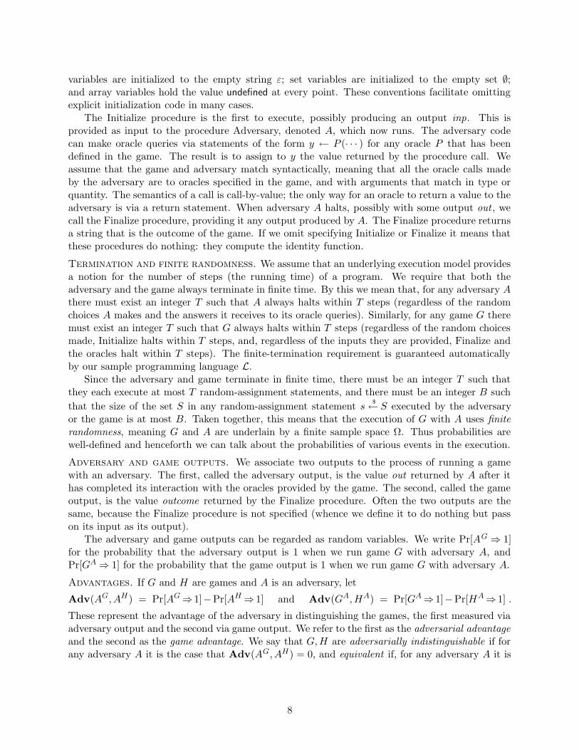
variables are initialized to the empty string ε; set variables are initialized to the empty set ∅;and array variables hold the value undefined at every point. These conventions facilitate omittingexplicit initialization code in many cases.

The Initialize procedure is the first to execute, possibly producing an output inp. This isprovided as input to the procedure Adversary, denoted A, which now runs. The adversary codecan make oracle queries via statements of the form y ← P (· · · ) for any oracle P that has beendefined in the game. The result is to assign to y the value returned by the procedure call. Weassume that the game and adversary match syntactically, meaning that all the oracle calls madeby the adversary are to oracles specified in the game, and with arguments that match in type orquantity. The semantics of a call is call-by-value; the only way for an oracle to return a value to theadversary is via a return statement. When adversary A halts, possibly with some output out , wecall the Finalize procedure, providing it any output produced by A. The Finalize procedure returnsa string that is the outcome of the game. If we omit specifying Initialize or Finalize it means thatthese procedures do nothing: they compute the identity function.

Termination and finite randomness. We assume that an underlying execution model providesa notion for the number of steps (the running time) of a program. We require that both theadversary and the game always terminate in finite time. By this we mean that, for any adversary Athere must exist an integer T such that A always halts within T steps (regardless of the randomchoices A makes and the answers it receives to its oracle queries). Similarly, for any game G theremust exist an integer T such that G always halts within T steps (regardless of the random choicesmade, Initialize halts within T steps, and, regardless of the inputs they are provided, Finalize andthe oracles halt within T steps). The finite-termination requirement is guaranteed automaticallyby our sample programming language L.

Since the adversary and game terminate in finite time, there must be an integer T such thatthey each execute at most T random-assignment statements, and there must be an integer B such

that the size of the set S in any random-assignment statement s$

← S executed by the adversaryor the game is at most B. Taken together, this means that the execution of G with A uses finiterandomness, meaning G and A are underlain by a finite sample space Ω. Thus probabilities arewell-defined and henceforth we can talk about the probabilities of various events in the execution.

Adversary and game outputs. We associate two outputs to the process of running a gamewith an adversary. The first, called the adversary output, is the value out returned by A after ithas completed its interaction with the oracles provided by the game. The second, called the gameoutput, is the value outcome returned by the Finalize procedure. Often the two outputs are thesame, because the Finalize procedure is not specified (whence we define it to do nothing but passon its input as its output).

The adversary and game outputs can be regarded as random variables. We write Pr[AG⇒ 1]for the probability that the adversary output is 1 when we run game G with adversary A, andPr[GA⇒ 1] for the probability that the game output is 1 when we run game G with adversary A.

Advantages. If G and H are games and A is an adversary, let

Adv(AG, AH) = Pr[AG⇒1]−Pr[AH⇒ 1] and Adv(GA,HA) = Pr[GA⇒ 1]−Pr[HA⇒1] .

These represent the advantage of the adversary in distinguishing the games, the first measured viaadversary output and the second via game output. We refer to the first as the adversarial advantageand the second as the game advantage. We say that G,H are adversarially indistinguishable if forany adversary A it is the case that Adv(AG, AH) = 0, and equivalent if, for any adversary A it is

8

the case that Adv(GA,HA) = 0. We will often use the fact that

Adv(AG, AI) = Adv(AG, AH) + Adv(AH , AI) (1)

Adv(GA, IA) = Adv(GA,HA) + Adv(HA, IA) (2)

for any games G,H, I and any adversary A. These will be referred to as the triangle equalities.We will usually be interested in adversarial advantage (eg, this is the case in the game-playing

proof of the PRP/PRF Switching Lemma). Game advantage is useful when we are interested inhow the adversary’s output relates to some game variable such as a hidden bit chosen by the game(this happens in our proof of the security of OAEP).

Identical-until-bad games. We are interested in programs that are syntactically identical exceptfor statements that follow the setting of a flag bad to true. Somewhat more precisely, let G and Hbe programs and let bad be a flag that occurs in both of them. Then we say that G and Hare identical-until-bad if their code is the same except that there might be places where G has astatement bad ← true, S while game H has a corresponding statement bad ← true, T for some Tthat is different from S. As an example, in the games S0 and S1 from Figure 6, the former has the

empty statement following bad ← true while in S1 we have Y$

← image(π) following bad ← true.Since this is the only difference in the programs, the games are identical-until-bad . One could alsosay that G and H are are identical-until-bad if one has the statement if bad then S where the otherhas the empty statement, for this can be rewritten in the form above.

A fully formal definition of identical-until-bad requires one to pin down the programming lan-guage and talk about the parse trees of programs in the language. We establish the needed languagein Appendix C but, in fact, such formality isn’t needed in applications: for any two games one writesdown, whether or not they are identical-until-bad is obvious. We emphasize that identical-until-badis a purely “syntactic” requirement.

We write Pr[AG sets bad ] or Pr[GA sets bad ] to refer to the probability that the flag bad is true

at the end of the execution of the adversary A with game G, namely at the point when the Finalizeprocedure terminates. It is easy to see that, for any flag bad , identical-until-bad is an equivalencerelation on games. When we say that a sequence of games G1, G2, . . . are identical-until-bad , wemean that each pair of games in the sequence are identical-until-bad .

The fundamental lemma. The fundamental lemma says that the advantage that an adversarycan obtain in distinguishing a pair of identical-until-bad games is at most the probability that itsexecution sets bad in one of the games (either game will do).

Lemma 1 [Fundamental lemma of game-playing] Let G and H be identical-until-bad games andlet A be an adversary. Then

Adv(AG, AH) ≤ Pr[AG sets bad ] and (3)

Adv(GA,HA) ≤ Pr[GA sets bad ] . (4)

More generally, let G,H, I be identical-until-bad games. Then

∣

∣Adv(AG, AH)∣

∣ ≤ Pr[AI sets bad ] and (5)∣

∣Adv(GA,HA)∣

∣ ≤ Pr[IA sets bad ] . (6)

Proof: Statement (3) follows from (4) by applying the latter to games G′,H ′ formed by replacingthe Finalize procedure of games G,H, respectively, with the trivial one that simply returns the

9

adversary output. Similarly, (5) follows from (6). We will now prove (4) and then derive (6) fromit.

We have required that the adversary and game always terminate in finite time, and also that there

is an integer that bounds the size of any set S in any random-assignment statement s$

← S executedby the adversary or game. This means that there exists an integer b such that the execution ofG with A and the execution of H with A perform no more than b random-assignment statements,each of these sampling from a set of size at most b. Let C = Coins(A,G,H) = [1 .. b!]b be the setof b-tuples of numbers, each number between 1 and b!. We call C the coins for (A,G,H). Forc = (c1, . . . , cb) ∈ C, the execution of G with A on coins c is defined as follows: on the ith random-

assignment statement, call it X$

← S, if S = a0, . . . , am−1 is nonempty and a0 < a1 < · · · < am−1

in lexicographic order then let X take on the value aci mod m. If S = ∅ then let X take on thevalue undefined. This way to perform random-assignment statements is done regardless of whetherit is A or one of the procedures from G that is is performing the random-assignment statement.Notice that m will divide b! and so if c is chosen at random from C then the mechanism above willreturn a point X drawn uniformly from S, and also the return values for each random-assignmentstatement are independent. For c ∈ C we let GA(c) denote the output of G when G is executedwith A on coins c. We define the execution of H with A on coins c ∈ C, and HA(c), similarly.

Let CGone = c ∈ C : GA(c)⇒ 1 be the set of coins c ∈ C such that G outputs 1 when executedwith A on coins c. Partition CGone into CG bad

one and CG goodone , where CG bad

one is the set of all c ∈ CGone

such that the execution of G with A on coins c sets bad and CG goodone = CGone \ CGbad

one . Similarlydefine CH one, CH bad

one and CH goodone . Observe that because games G and H are identical-until-bad ,

an element c ∈ C is in CG goodone iff it is in CH good

one . Thus these sets are equal and in particular havethe same size. Now we have

Pr[GA⇒ 1]− Pr[AH ⇒ 1] =|CGone|

|C|−|CH one|

|C|=|CG bad

one |+ |CG goodone | − |CH good

one | − |CH badone |

|C|

=|CG bad

one | − |CH badone |

|C|≤|CG bad

one |

|C|≤|CGbad|

|C|= Pr[GA sets bad ] .

This completes the proof of (4). Now, if G,H are identical-until-bad then (4) tells us that

Adv(GA,HA) ≤ Pr[GA sets bad ] and Adv(HA, GA) ≤ Pr[HA sets bad ] .

However, if G,H, I are all identical-until-bad , then Proposition 2 says that

Pr[GA sets bad ] = Pr[HA sets bad ] = Pr[IA sets bad ] .

Thus we have established (6).

We have used finite randomness in our proof of the Fundamental Lemma, but we comment that thisis more for simplicity than necessity: probabilities over the execution of G with A can be definedquite generally, even when the underlying sample space is infinite, and the Fundamental Lemmacan still be proved. But we have never encountered any situation where such an extension is useful.

After bad is set, nothing matters. One of the most common manipulations of games alonga game chain is to change what happens after bad gets set to true. Often one expunges code thatfollows the setting of bad , as we did in the PRP/PRF Switching Lemma,but it is also fine to insertalternative code. Any modification following the setting of bad leaves unchanged the probability ofsetting bad , as the following result shows.

Proposition 2 [After bad is set, nothing matters] Let G and H be identical-until-bad games.Let A be an adversary. Then Pr[GA sets bad ] = Pr[HA sets bad ].

10

Proof: Using the definition from the proof of Lemma 1, fix coins C = Coins(A,G,H) and ex-ecute GA and HA in the manner we described using these coins. Let CG bad ⊆ C be the coinsthat result in bad getting set to true when we run GA, and let CH bad ⊆ C be the coins thatresult in bad getting set to true when we run HA. Since G and H are identical-until-bad , eachc ∈ C causes bad to be set to true in GA iff it causes bad to be set to true in HA. ThusCGbad = CH bad and hence |CGbad| = |CH bad| and |CGbad|/|C| = CH bad|/|C|, which is to saythat Pr[GA sets bad ] = Pr[HA sets bad ].

Besides the lemma above, many other ways to manipulate games are illustrated by our examplesand our discussion in Section D.

Game inputs. The setting discussed above can be extended to allow a game to take an inputparameter: the Initialize procedure would take an optional input that is a string parameter input .The adversary and game outputs will now be denoted Pr[AG(input)⇒ 1] and Pr[GA(input)⇒ 1]respectively. Similarly, the advantages become Adv(AG(input), AH(input)) and Adv(GA(input),HA(input)), these being defined in the obvious ways. The definition of identical-until-bad obviouslyextends to games with inputs, as does the Fundamental Lemma.

We can imagine that it might be convenient for games to have inputs, for example in theasymptotic setting where input might be the security parameter, but our experience has been thatit is not really necessary. Rather than giving a game an input input , we can usually imagine afamily of games, one for each value of input , and reason about these; since the games are involvedonly in the analysis, this usually suffices. Accordingly our treatment of games omits explicit gameinputs.

3 The Security of Three-Key Triple-Encryption

Triple encryption goes back to the early attempts to strengthen DES against key-search attacks [19].We now show that the method increases security, in the ideal-cipher model, resolving a long-standingopen problem.

Definitions. Let E : 0, 1k × 0, 1n → 0, 1n be a blockcipher with key length k and blocklength n. For K ∈ 0, 1k and X ∈ 0, 1n let EK(X) = E(K,X). Let E−1 : 0, 1k × 0, 1n →0, 1n be the blockcipher that is the inverse of E. We also denote it by D. We associate to E twoblockciphers formed by composition. Denoted Cascadeeee

E ,CascadeedeE : 0, 13k ×0, 1n → 0, 1n,

they are defined as

CascadeeeeE (K0K1K2, X) = EK2

(EK1(EK0

(X))) and

CascadeedeE (K0K1K2, X) = EK2

(DK1(EK0

(X)))

for all K0,K1,K2 ∈ 0, 1k and X ∈ 0, 1n. These blockciphers have key length 3k and block

length n and are sometimes referred to as the three-key forms of triple encryption. We will callthe two methods EEE and EDE, respectively. There is also a two-key variant of triple encryption,obtained by setting K0 = K2, but we do not investigate it since the method admits comparativelyefficient attacks [34].

We will be working in the ideal-blockcipher model, as in works like [3, 22, 30]. Let Bloc(k, n)

be the set of all blockciphers E : 0, 1k × 0, 1n → 0, 1n. Thus E$

← Bloc(k, n) means thatEK : 0, 1n → 0, 1n is a random permutation on n-bit strings for each K ∈ 0, 1k. We con-sider an adversary A that can make four types of oracle queries: T (X), T

−1(Y ), E(K,X), and

11

E−1(K,Y ), where X,Y ∈ 0, 1n and K ∈ 0, 1k. (As for our syntax, T , T

−1, E, E−1 are for-

mal symbols, not specific functions.) The advantage of A against EEE and the maximal advantageagainst EEE obtainable using q queries are defined as

Adveeek,n(A) = Adv(AC0 , AR0) and Adveee

k,n(q) = maxA

Adveeek,n(A)

where the games C0, R0 are shown in Figure 3 and the maximum is over all adversaries A thatmake at most q oracle queries (that is, a total of q across all oracles). The advantage of A mea-sures its ability to tell whether T (·) is a random permutation or is Cascadeeee

E (K0K1K2, · ) for

K0K1K2$

←0, 13k, when E realizes a random blockcipher E$

← Bloc(k, n) and T−1,E−1 realize

inverses of T ,E, respectively.Define the query threshold QTheee

1/2(k, n) as the largest integer q for which Adveeek,n(q) ≤ 1/2.

We will speak of EEE being secure up to QTheee1/2(k, n) queries. Let Advede

k,n(A),Advedek,n(q), and

QThede1/2(k, n) be defined in the analogous way.

Results. The main result of this section is the following:

Theorem 3 [Security of triple-encryption] Let k, n ≥ 2. Let α = max(2e2k−n, 2n + k). Then

Adveeek,n(q) ≤ 4α

q2

23k+ 10.7

( q

2k+n/2

)2/3+

12

2k. 2 (7)

We display the result graphically in Figure 1 for DES parameters k = 56 and n = 64. Our boundimplies that QTheee

1/2(k, n) is, very roughly, about 2k+min(k,n)/2, meaning that EEE is secure up tothis many queries. We remark that Lucks [31] provides a key-recovery attack on EEE that succeedsin about 2k+n/2 queries, indicating that our threshold value is reasonably tight for n ≤ k.

For EDE the result is the same, meaning that Advedek,n(q) is also bounded by the quantity on

the right-hand-side of (7). This can be shown by mostly-notational modifications to the proof ofTheorem 3.

Conventions. The rest of this section, as well as Appendix E, is for proving Theorem 3. We beginwith some conventions. Recall that an adversary A against EEE or EDE can make oracle queriesT (X), T

−1(Y ), E(K,X), or E−1(K,Y ) for any X,Y ∈ 0, 1n and K ∈ 0, 1k. We will assume

that any adversary against EEE or EDE is deterministic and never makes a redundant query. Aquery is redundant if it has been made before; a query T

−1(Y ) is redundant if A has previouslyreceived Y in answer to a query T (X); a query T (X) is redundant if A has previously received Xin answer to a query T

−1(Y ); a query E−1(K,Y ) is redundant if A has previously received Y

in answer to a query E(K,X); a query E(K,X) is redundant if A has previously received X inanswer to a query E

−1(K,Y ). Assuming A to be deterministic and not to ask redundant queriesis without loss of generality in the sense that for any A that asks q queries there is an A ′ askingat most q queries that satisfies these assumptions and achieves the same advantage as A. Finally,recall that our general conventions imply that A never asks a query with arguments outside of theintended domain, meaning 0, 1k for keys and 0, 1n for messages. We say that an adversary issimplified if it does not make T (·), T

−1(·) queries (that is, it makes only E(·, ·), E−1(·, ·) queries).

Simplifying the adversary. The first step in our proof is to reduce the problem of boundingthe advantage of an adversary against EEE to the problem of bounding advantage for a simplifiedadversary that aims to distinguish between a new pair of games (obviously not the original pairof games since an adversary can get no advantage in distinguishing R0 and C0 if it makes no T (·)or T

−1(·) queries). Consider the games in Figure 3. The R-games (where R stands for random)omit the boxed assignment statements while the C-games (where C stands for construction) includethem. Distinctk

3 denotes the set of all triples (K0,K1,K2) ∈ (0, 1k)3 such that K0 6= K1 and

12

procedure Initialize Game R0 Game C0

K0, K1, K2

$←0, 1k, E

$← Bloc(k, n), T

$← Perm(n), T ← EK2

EK1EK0

procedure T (P ) procedure T−1(S)

return T [P ]return T−1[S]

procedure E(K, X) procedure E−1(K, Y )

return EK [X ] return E−1

K [Y ]


(K0, K1, K2)$←Distinctk

3 , E$←Bloc(k, n), T

$←Perm(n), T←EK2

EK1EK0


return T [P ]return T−1[S]



K [Y ]


(K0, K1, K2)$←Distinctk

3 , E$←Bloc(k, n), T

$←Perm(n), EK2

←T E−1

K0E−1

K1


return T [P ] return T−1[S]



K [Y ]

procedure Initialize Game R2 Game CT

300 (K0, K1, K2)$← Distinctk

3 , E$← Bloc(k, n), EK2

← T E−1

K0E−1

K1


310 return EK [X ] 320 return E−1

K [Y ]

Figure 3: Games used for triple encryption. The Ci games include the boxed statements, the Ri games donot.

K1 6= K2 and K0 6= K2. Game CT is parameterized by a permutation T ∈ Perm(n), meaning weare effectively defining one such game for every T . Now we claim the following:

Lemma 4 Let A1 be an adversary that makes at most q oracle queries. Then there is a simplifiedadversary B and a permutation S ∈ Perm(n) such that

Adveeek,n(A1) ≤ Adv(BCS , BR2) +

6

2k.

Furthermore, B also makes at most q oracle queries.

Proof: The only change between games R0 and R1 is to draw the keys K0,K1,K2 from Distinctk3

rather than from (0, 1k)3, and similarly for games C0 and C1. So

Adv(AC0

1 , AC1

1 ) ≤3

2kand Adv(AR1

1 , AR0

1 ) ≤3

2k.

(The above can easily be shown with games, but it is so simple that we do not bother.) Now using

13

triangle equality (1) and the above we have

Adveeek,n(A1) = Adv(AC0

1 , AR0

1 ) = Adv(AC0

1 , AC1

1 ) + Adv(AC1

1 , AR1

1 ) + Adv(AR1

1 , AR0

1 )

≤ Adv(AC1

1 , AR1

1 ) +6

2k. (8)

Game C2 is obtained from game C1 as follows: instead of defining T as E2 E1 E0 for randomE0, E1, E2, we define E2 as T E−1

K0EK1

for random T,EK0, EK1

. These two processes are identical,and so

Adv(AC1

1 , AR1

1 ) = Adv(AC2

1 , AR1

1 ) . (9)

Game CT is parameterized by a permutation T ∈ Perm(n). For any such T we consider an adversaryAT that has T hardwired in its code and is simplified, meaning can make queries E(K,X) andE

−1(K,Y ) only. This adversary runs A1, answering the latter’s E(K,X) and E−1(K,Y ) queries

via its own oracles, and answering T (X) and T−1(Y ) queries using T . Note that AT makes at

most q oracle queries. Choose S ∈ Perm(n) such that

Adv(ACS

S , AR2

S ) = maxT∈Perm(n)

Adv(ACT

T , AR2

T )

and let B = AS . Then, with the expectation taken over T$

← Perm(n) we have

Adv(AC2

1 , AR1

1 ) = E[

Adv(ACT

T , AR2

T )]

≤ Adv(ACS

S , AR2

S ) = Adv(BCS , BR2) . (10)

This concludes the proof.

Pseudorandomness of three correlated permutations. Towards bounding the advantageof a simplified adversary in distinguishing between games C3 and R3 we posit a new problem.Consider games G and H defined in Figure 4. An adversary may make queries Π(i,X) or Π−1(i, Y )where i ∈ 0, 1, 2 and X,Y ∈ 0, 1n. The oracles realize three permutations and their inverses,the function realized by Π−1(i, · ) being the inverse of the one realizing Π(i, · ) for all i ∈ 0, 1, 2.In both games permutations π0, π1 underlying Π(0, · ) and Π(1, · ) are random and independentpermutations. In game G, the permutation π2 underlying Π(2, · ) is also random and independentof π0 and π1, but in game H it is equal to π−1

1 π−10 .

Notice that it is easy for an adversary to distinguish between games G and H by makingqueries that form a “chain” of length three: for any P ∈ 0, 1n, let the adversary ask and be givenQ ← π0(P ), then R ← π1(Q), then P ′ ← π2(R), and then have the adversary output 1 if P = P ′

(a “triangle” has been found) or 0 if P 6= P ′ (the “three-chain” is not in fact a triangle). Whatwe will establish is that, apart from such behavior—extending a known “2-chain”—the adversaryis not able to gain much advantage. To capture this, as the adversary A makes its queries andgets replies, the games form an edge-labeled directed graph G. The graph, whose vertex set is

0, 1n, is initially without edges (we omit explicit initialization for the graph G). An arc Xi−→Y

is created when a query Π(i,X) returns the value Y or a query Π−1(i, Y ) returns the value X.The boolean flag x2ch is set in the games if the adversary “extends a 2-chain,” meaning that a

path Pi+1−→Q

i+2−→R exists in the graph and the adversary asks either Π(i, R) or Π−1(i, P ), where

the indicated addition is modulo 3. We will be interested in the game outputs rather than theadversary outputs. If the flag x2ch gets set to true then the adversary effectively loses: the game’soutput is defined as a constant (rather than the adversary’s output) and the adversary will gain noadvantage form this run. We comment that we have described games G and H as working with agraph, which is not actually a type in our formal programming language L, but it is easy to recastthe games to use a set instead of a graph, it is simply that the code may be slightly less readable.We show, again using a game-based proof, that:

14

procedure Initialize Game G Game H

π0, π1, π2

$← Perm(n), π2 ← π−1

1 π−10

procedure Π(i, X) procedure Π−1(i, Y )

if ∃ Pi+1−→Q

i+2−→X ∈ G then x2ch← true if ∃ Y

i+1−→Q

i+2−→R ∈ G then x2ch← true

add Xi−→ πi[X ] to G add π−1

i [Y ]i−→ Y to G

return πi[X ] return π−1

i [Y ]

procedure Finalize(out)if x2ch then return 1 else return out

procedure E(K, X) procedure E−1(K, Y ) Game L

return EK [X ]$← image(EK) E−1

K [Y ]$← domain(EK)

procedure Finalize

K0, K1, K2

$←0, 1k

if (∃P ) [EK2[EK1

[EK0[P ]]]] then bad ← true

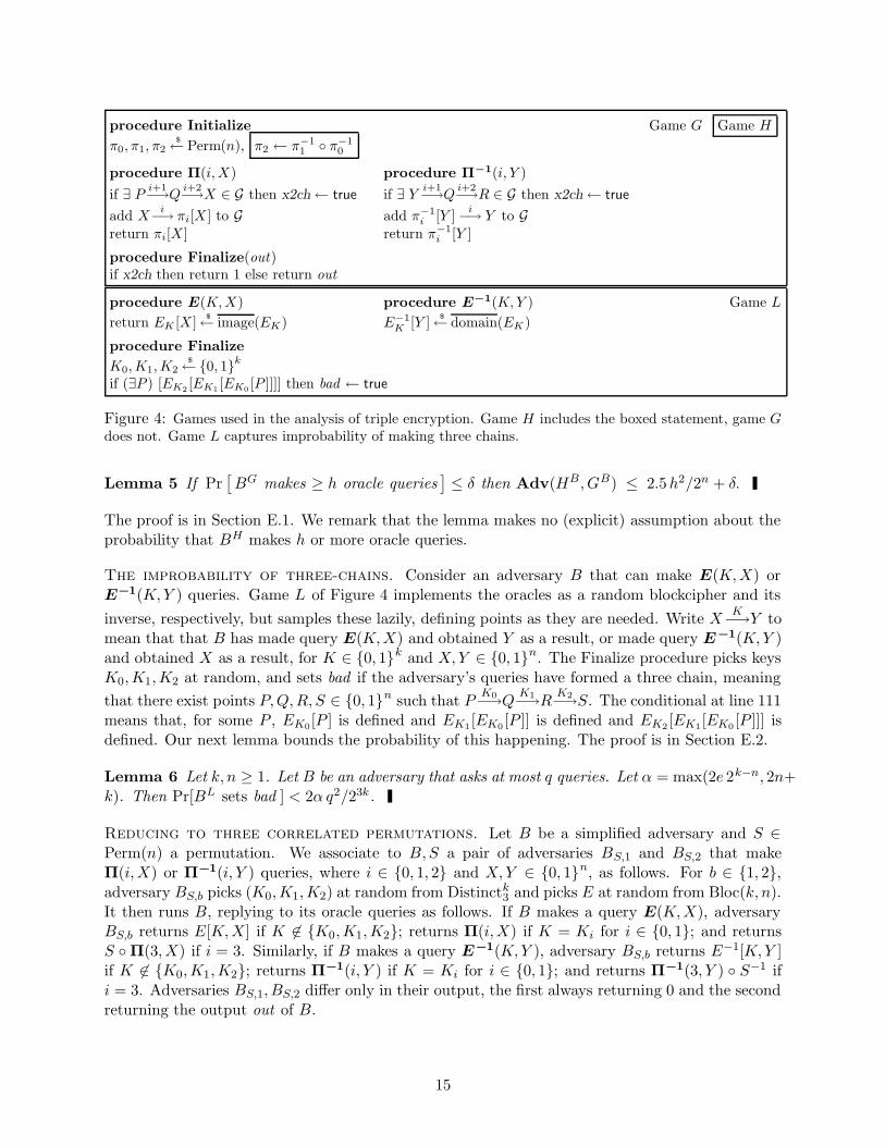
Figure 4: Games used in the analysis of triple encryption. Game H includes the boxed statement, game Gdoes not. Game L captures improbability of making three chains.

Lemma 5 If Pr[

BG makes ≥ h oracle queries]

≤ δ then Adv(HB , GB) ≤ 2.5h2/2n + δ.

The proof is in Section E.1. We remark that the lemma makes no (explicit) assumption about theprobability that BH makes h or more oracle queries.

The improbability of three-chains. Consider an adversary B that can make E(K,X) orE

−1(K,Y ) queries. Game L of Figure 4 implements the oracles as a random blockcipher and its

inverse, respectively, but samples these lazily, defining points as they are needed. Write XK−→Y to

mean that that B has made query E(K,X) and obtained Y as a result, or made query E−1(K,Y )

and obtained X as a result, for K ∈ 0, 1k and X,Y ∈ 0, 1n. The Finalize procedure picks keysK0,K1,K2 at random, and sets bad if the adversary’s queries have formed a three chain, meaning

that there exist points P,Q,R, S ∈ 0, 1n such that PK0−→Q

K1−→RK2−→S. The conditional at line 111

means that, for some P , EK0[P ] is defined and EK1

[EK0[P ]] is defined and EK2

[EK1[EK0

[P ]]] isdefined. Our next lemma bounds the probability of this happening. The proof is in Section E.2.

Lemma 6 Let k, n ≥ 1. Let B be an adversary that asks at most q queries. Let α = max(2e 2k−n, 2n+k). Then Pr[BL sets bad ] < 2α q2/23k.

Reducing to three correlated permutations. Let B be a simplified adversary and S ∈Perm(n) a permutation. We associate to B,S a pair of adversaries BS,1 and BS,2 that makeΠ(i,X) or Π−1(i, Y ) queries, where i ∈ 0, 1, 2 and X,Y ∈ 0, 1n, as follows. For b ∈ 1, 2,adversary BS,b picks (K0,K1,K2) at random from Distinctk

3 and picks E at random from Bloc(k, n).It then runs B, replying to its oracle queries as follows. If B makes a query E(K,X), adversaryBS,b returns E[K,X] if K 6∈ K0,K1,K2; returns Π(i,X) if K = Ki for i ∈ 0, 1; and returnsS Π(3, X) if i = 3. Similarly, if B makes a query E

−1(K,Y ), adversary BS,b returns E−1[K,Y ]if K 6∈ K0,K1,K2; returns Π−1(i, Y ) if K = Ki for i ∈ 0, 1; and returns Π−1(3, Y ) S−1 ifi = 3. Adversaries BS,1, BS,2 differ only in their output, the first always returning 0 and the secondreturning the output out of B.

15

procedure Initialize Game R3

500 (K0, K1, K2)$←Distinctk

3 , E$←Bloc(k, n), EK2

←SE−1

K0E−1

K1Game DS

procedure E(K, X)510 if ∃ i ∈ 0, 1, 2 such that K = Ki then511 Q← E−1

Ki+2[X ], P ← E−1

Ki+1[Q]

512 if Pi+1−→Q

i+2−→X then x2ch← true

513 Add arc Xi−→EK [X ]

514 return EK [X ]

procedure E−1(K, Y )

520 if ∃ i ∈ 0, 1, 2 such that K = Ki then521 Q← EKi+1

[Y ], R← EKi+2[Q]

522 if Yi+1−→Q

i+2−→R then x2ch← true

523 Add arc E−1

K [Y ]i−→Y

524 return E−1

K [Y ]

procedure Finalize530 if x2ch then return 1 else return out

Figure 5: Games used in the triple-encryption analysis. Game DS includes the boxed statement, game R3

does not.

Lemma 7 Let B be a simplified adversary that makes at most q oracle queries, and let S ∈Perm(n). Let BS,1, BS,2 be defined based on B,S as above. Let K = 2k. Then for b ∈ 1, 2and every real number c > 0,

Pr[

BGS,b makes ≥ 3cq/K oracle queries

]

≤1

c.

The proof is in Appendix E.3.

Proof of Theorem 3: We now show how to prove Theorem 3 given the above lemmas. Let A bean adversary against EEE that makes at most q oracle queries. Let B be the simplified adversary,and S the permutation, given by Lemma 4, and let BS,1, BS,2 be the adversaries associated to it asdescribed above. Consider the games R3, DS of Figure 5 and note that

Pr[DBS sets x2ch ] = Pr[HBS,1 ⇒ 1] and Pr[RB

3 sets x2ch ] = Pr[GBS,1 ⇒ 1]Pr[DB

S ⇒ 1] = Pr[HBS,2 ⇒ 1] and Pr[RB3 ⇒ 1] = Pr[GBS,2 ⇒ 1] .

(11)

16

Let α = max(2e2k−n, 2n + k). Then for any c > 0 we have the following:

Adveeek,n(A)

≤ Adv(BCS , BR2) +6

2k(12)

= Adv(CBS , DB

S ) + Adv(DBS , RB

3 ) + Adv(RB3 , RB

2 ) +6

2k(13)

≤ Pr[

DBS sets x2ch

]

+ Pr[

RB3 sets x2ch

]

+ Adv(DBS , RB

3 ) +6

2k(14)

= 2 · Pr[

RB3 sets x2ch

]

+ Pr[

DBS sets x2ch

]

− Pr[

RB3 sets x2ch

]

+ Adv(DBS , RB

3 ) +6

2k

= 2 · Pr[

RB3 sets x2ch

]

+ Adv(HBS,1 , GBS,1) + Adv(HBS,2 , GBS,2) +6

2k(15)

≤ 2 ·

(

3

2k+ Pr[BL sets bad ]

)

+ Adv(HBS,1 , GBS,1) + Adv(HBS,2 , GBS,2) +6

2k(16)

≤ 2

(

3

2k+ 2α

q2

23k

)

+5

2n

(

3cq

2k

)2

+2

c+

6

2k(17)

Above, (12) is by Lemma 4, and (13) is by triangle equality (2). To justify (14) we note thatgame CS can be easily transformed into an equivalent game such that this game and game DS areidentical-until-bad , and, similarly, game R2 can be easily transformed into an equivalent game suchthat this game and game R3 are identical-until-bad , and thus (14) follows from the FundamentalLemma. To justify (15) we use (11). To justify (16) we note that the probability that RB

3 extendsa 2-chain is at most the probability that LB forms a 3-chain. The extra term is because L picks thekeys K0,K1,K2 independently at random while R3 picks them from Distinctk

3 . To get (17) we firstapplied Lemma 6 and then, for each b ∈ 1, 2, applied Lemma 5 in conjunction with Lemma 7.Now, since the above is true for any c > 0, we pick a particular one that minimizes the functionf(c) = 45 c2q2 2−n−2k + 2c−1. The derivative is f ′(c) = 90 cq2 2−n−2k − 2c−2, and the only realroot of the equation f ′(c) = 0 is c = (2n+2k/45q2)1/3, for which we have f(c) = 3(45q2/2n+2k)1/3.Plugging this into the above yields (7) and concludes the proof of Theorem 3.

Acknowledgments

We thank Tadayoshi Kohno for permission to use his observations about the standard proof of thePRP/PRF Switching Lemma noted in Section A and Appendix B.

Mihir Bellare was supported by NSF 0098123, ANR-0129617, NSF 0208842, and an IBM FacultyPartnership Development Award. Phil Rogaway was supported by NSF 0208842 and a gift fromIntel Corp. Much of the work on this paper was carried out while Phil was hosted by Chiang MaiUniversity, Thailand.

References

[1] M. Abe, R. Gennaro, K. Kurosawa and V. Shoup. Tag-KEM/DEM: A new framework forhybrid encryption and a new analysis of Kurosawa-Desmedt KEM. Eurocrypt ’05.

[2] L. Adleman. Two theorems on random polynomial time. FOCS 78.[3] W. Aiello, M. Bellare, G. Di Crescenzo, and R. Venkatesan. Security amplification by compo-

sition: the case of doubly-iterated, ideal ciphers. Crypto ’98.

17

[4] M. Bellare and S. Goldwasser. New paradigms for digital signatures and message authentica-tion based on non-interactive zero knowledge proofs. Crypto 89, pp. 194–211, 1989.

[5] M. Bellare, J. Kilian, and P. Rogaway. The security of the cipher block chaining messageauthentication code. Journal of Computer and System Sciences (JCSS), vol. 61, no. 3, pp. 362–399, 2000. Earlier version in Crypto ’94.

[6] M. Bellare, T. Krovetz, and P. Rogaway. Luby-Rackoff backwards: increasing security bymaking block ciphers non-invertible. Eurocrypt ’98.

[7] M. Bellare, K. Pietrzak, and P. Rogaway. Improved security analyses for CBC MACs.Crypto 05.

[8] M. Bellare and P. Rogaway. Optimal asymmetric encryption. Eurocrypt ’94.[9] M. Bellare and P. Rogaway. Random oracles are practical: a paradigm for designing efficient

protocols. ACM CCS ’93.[10] M. Bellare, P. Rogaway, and D. Wagner. The EAX mode of operation (a two-pass authenti-

cated encryption scheme). FSE ’04

[11] D. Bernstein. A short proof of the unpredictability of cipher block chaining. Manuscript,January 2005. Available on Bernstein’s web page.

[12] J. Black and P. Rogaway. CBC MACs for arbitrary-length messages: the three-key construc-tions. Crypto ’00.

[13] J. Black and P. Rogaway. A block-cipher mode of operation for parallelizable message authen-tication. Eurocrypt ’02.

[14] J. Black, P. Rogaway, and T. Shrimpton. Encryption-scheme security in the presence of key-dependent messages. SAC 2002.

[15] D. Boneh. Simplified OAEP for the RSA and Rabin functions. Crypto ’01.[16] J. Camenisch and V. Shoup. Practical verifiable encryption and decryption of discrete logs.

Crypto ’03.[17] R. Cramer and V. Shoup. Design and analysis of practical public-key encryption schemes

secure against adaptive chosen ciphertext attack. SIAM J. of Computing, vol. 33, pp. 167–226, 2003.

[18] R. Cramer and V. Shoup. Universal hash proofs and a paradigm for adaptive chosen ciphertextsecure public key encryption. Eurocrypt ’02.

[19] W. Diffie and M. Hellman. Exhaustive cryptanalysis of the data encryption standard. Com-

puter, vol. 10, pp. 74–84, 1977.[20] Y. Dodis, R. Gennaro, J. Hastad, H. Krawczyk, and T. Rabin. Randomness extraction and

key derivation using the CBC, Cascade, and HMAC modes. Crypto ’04.[21] S. Even and O. Goldreich. On the power of cascade ciphers. ACM Transactions on Computer

Systems, vol. 3, no. 2, pp. 108–116, 1985.[22] S. Even and Y. Mansour. A construction of a cipher from a single pseudorandom permutation.

Asiacrypt ’91. LNCS 739, Springer-Verlag, pp. 210–224, 1992.[23] E. Fujisaki, T. Okamoto, D. Pointcheval, and J. Stern. RSA-OAEP is secure under the RSA

assumption. J. of Cryptology, vol. 17, no. 2, pp. 81–104, 2004.[24] S. Goldwasser and S. Micali. Probabilistic encryption. J. Comput. Syst. Sci., vol. 28, no. 2,

pp. 270–299, 1984. Earlier version in STOC ’82.[25] S. Halevi. A plausible approach to computer-aided cryptographic proofs. Cryptology ePrint

archive report 2005/181, 2005.[26] S. Halevi and P. Rogaway. A parallelizable enciphering mode. CT-RSA ’04.[27] S. Halevi and P. Rogaway. A tweakable enciphering mode. Crypto ’03. LNCS 2729, pp. 482–

499, 2004.[28] C. Hall, D. Wagner, J. Kelsey, and B. Schneier. Building PRFs from PRPs. Available on

18

Wagner’s web page. Earlier version in Crypto ’98.[29] E. Jaulmes, A. Joux, and F. Valette. On the security of randomized CBC-MAC beyond the

birthday paradox limit: a new construction. FSE ’02. LNCS 2365, pp. 237–251, 2002.[30] J. Kilian and P. Rogaway. How to protect DES against exhaustive key search (an analysis of

DESX). J. of Cryptology, vol. 14, no. 1, pp. 17–35, 2001. Earlier version in Crypto ’96.[31] S. Lucks. Attacking triple encryption. FSE ’98. LNCS 1372, pp. 239–253, 1998.[32] U. Maurer. Indistinguishability of random systems. Eurocrypt ’02. LNCS 2332, Springer-

Verlag, pp. 110–132, 2002.[33] U. Maurer and J. Massey. Cascade ciphers: the importance of being first. J. of Cryptology,

vol. 6, no. 1, pp. 55–61, 1993.[34] R. Merkle and M. Hellman. On the security of multiple encryption. Communications of the

ACM, vol. 24, pp. 465–467, 1981.[35] R. Motwani and P. Raghavan. Randomized Algorithms. Cambridge University Press, 1995.[36] National Institute of Standards and Technology. FIPS PUB 46-3, Data Encryption Standard

(DES), 1999. Also ANSI X9.52, Triple Data Encryption Algorithm modes of operation, 1998,and other standards.

[37] E. Petrank and C. Rackoff. CBC MAC for real-time data sources. J. of Cryptology, vol. 13,no. 3, pp. 315–338, 2000.

[38] P. Rogaway. Authenticated-encryption with associated-data. ACM CCS ’02.[39] P. Rogaway. Efficient instantiations of tweakable blockciphers and refinements to modes OCB

and PMAC. Asiacrypt ’04.[40] P. Rogaway, M. Bellare, and J. Black. OCB: A block-cipher mode of operation for efficient

authenticated encryption. ACM Transactions on Information and System Security, vol. 6,no. 3, pp. 365–403, 2003. Earlier version in ACM CCS ’01.

[41] T. Schweinberger and V. Shoup. ACE: the advanced cryptographic engine. Cryptology ePrintreport 2000/022, 2000.

[42] C. Shannon. Communication theory of secrecy systems. Bell Systems Technical Journal,vol. 28, no. 4, pp. 656–715, 1949.

[43] V. Shoup. OAEP reconsidered. J. of Cryptology, vol. 15, no. 4, pp. 223–249, 2002. Earlierversion in Crypto ’01.

[44] V. Shoup. A proposal for an ISO standard for public key encryption. Cryptology ePrint report2001/112, 2001.

[45] V. Shoup. Sequences of games: a tool for taming complexity in security proofs. CryptologyePrint report 2004/332, November 30, 2004.

[46] V. Shoup. Using hash function as a hedge against chosen ciphertext attack. Eurocrypt ’00.[47] S. Vaudenay. Decorrelation over infinite domains: the encrypted CBC-MAC case. Communi-

cations in Information and Systems (CIS), vol. 1, pp. 75–85, 2001.[48] A. Yao. Theory and applications of trapdoor functions. FOCS 1982, pp. 80–91, 1982.

A The PRP/PRF Switching Lemma

The lemma. The natural and conventional assumption to make about a blockcipher is that itbehaves as a pseudorandom permutation (PRP). However, it usually turns out to be easier toanalyze the security of a blockcipher-based construction assuming the blockcipher is secure as apseudorandom function (PRF). The gap is then bridged (meaning, a result about the security ofthe construct assuming the blockcipher is a PRP is obtained) using the following lemma. In whatfollows, we denote by AP ⇒ 1 the event that adversary A, equipped with an oracle P , outputs

19

the bit 1. Let Perm(n) be the set of all permutations on 0, 1n and let Func(n) be the set ofall functions from 0, 1n to 0, 1n. We assume below that π is randomly sampled from Perm(n)and ρ is randomly sampled from Func(n).

Lemma 8 [PRP/PRF Switching Lemma] Let n ≥ 1 be an integer. Let A be an adversary thatasks at most q oracle queries. Then

|Pr [Aπ⇒ 1 ]− Pr [Aρ⇒ 1 ]| ≤q(q − 1)

2n+1.

In this section we point to some subtleties in the “standard” proof of this widely used result, asgiven for example in [5, 28], showing in particular that one of the claims made in these proofsis incorrect. We then show how to prove the lemma in a simple and correct way using games.This example provides a gentle introduction to the game-playing technique and a warning aboutperils of following ones intuition when dealing with conditional probability in provable-securitycryptography.

The standard proof. The standard analysis proceeds as follows. Let Coll (“collision”) be the

event that A, interacting with oracle ρ$

← Func(n), asks distinct queries X and X ′ that return thesame answer. Let Dist (“distinct”) be the complementary event. Now

Pr[Aπ⇒ 1] = Pr[Aρ⇒ 1 | Dist] (18)

since a random permutation is the same as a random function in which everything one obtains fromdistinct queries is distinct. Letting x be this common value and y = Pr[Aρ⇒ 1 | Coll] we have

|Pr[Aπ⇒ 1]− Pr[Aρ⇒ 1]| = |x− xPr[Dist]− y Pr[Coll]| = |x(1− Pr[Dist])− y Pr[Coll]|

= |xPr[Coll]− y Pr[Coll]| = |(x− y) Pr[Coll]| ≤ Pr[Coll]

where the final inequality follows because x, y ∈ [0, 1]. One next argues that Pr[Coll] ≤ q(q −1)/2n+1 and so the Switching Lemma follows.

Where is the error in the simple proof above? It’s at equation (18): it needn’t be the case thatPr[Aπ⇒1] = Pr[Aρ⇒1 | Dist], and the sentence we gave by way of justification was mathematicallymeaningless. Here is a simple example to demonstrate that Pr[Aπ ⇒ 1] can be different fromPr[Aρ⇒1 | Dist]. Let n = 1 and consider the following adversary A with oracle P : 0, 1 → 0, 1:

procedure Adversary Aif P (0) = 0 then return 1

else if P (1) = 1 then return 1 else return 0

We claim that

Pr[Aπ⇒ 1] = 1/2 and Pr[Aρ⇒ 1 | Dist] = 2/3 .

The first equation is true because there are two possibilities for (π(0), π(1)), namely (0, 1), (1, 0),and A returns 1 for one of them, namely (0, 1). On the other hand, there are four possibilitiesfor (ρ(0), ρ(1)), namely (0, 0), (0, 1), (1, 0), (1, 1). The event Aρ⇒ 1 ∧Dist is true for two of them,namely (0, 0), (0, 1), while the event Dist is true for three of them, namely (0, 0), (0, 1), (1, 0). ThusPr[Aρ⇒ 1 ∧Dist]/Pr[Dist] = 2/3.

Notice that the number of oracle queries made by the adversary of this counterexample varies,being either one or two, depending on the reply it receives to its first query. This turns out to becrucial in making equation (18) fail, in that if A always makes exactly q oracle queries (regardlessof A’s coins and the answers returned to its queries) then equation (18) is true. (This was pointedout by Kohno, and his argument is re-produced in Appendix B.) Since one can always first modify

20

procedure P (X) Game S0

100 Y$

← 0, 1n Game S1

101 if Y ∈ image(π) then bad ← true, Y$

← image(π)

102 return π[X]← Y

Figure 6: Games used in the proof of the Switching Lemma. Game S1 includes the boxed statement and S0

doesn’t.

A to make exactly q queries without altering Pr[Aρ⇒ 1] or Pr[Aπ ⇒ 1], we would be loath to saythat the proofs in [5, 28] are incorrect. But the authors make claim (18), and view it as “obvious,”without restricting the adversary to exactly q queries, masking a subtlety that is not apparent ata first (or even second) glance.

The fact that one can write something like (18) and people assume this to be correct, andeven obvious, suggests to us that the language of conditional probability may often be unsuitablefor thinking about and dealing with the kind of probabilistic scenarios that arise in cryptography.Games may more directly capture the desired intuition. Let us use them to give a correct proof.

Game-based proof. Assume without loss of generality (since A’s oracle is deterministic) that Anever asks an oracle query twice. We imagine answering A’s queries by running one of two games.

Instead of thinking of A as interacting with a random permutation oracle π$

← Perm(n), think of itas interacting with the Game S1 shown in Figure 6. Instead of thinking of A as interacting with a

random function oracle ρ$

← Func(n), think of A as interacting with the game S0 shown in the samefigure. Game S0 is game S1 without the boxed statement. By convention, the boolean variable badis initialized to false while the array π begins everywhere undefined. The games make available toA an oracle which has a formal name, in this case P . Adversary A can query this oracle with astring X ∈ 0, 1n, in which case the code following the procedure P (X) line is executed and thevalue in the return statement is provided to A as the response to its oracle query. As the gameruns, we fill-in values of π[X] with n-bit strings. At any point in time, we let image(π) be the setof all n-bit strings Y such that π[X] = Y for some X. Let image(π) be the complement of this setrelative to 0, 1n. Let AS ⇒ 1 denote the event that A outputs 1 in game S ∈ S0, S1.

Notice that the adversary never sees the flag bad . The flag will play a central part in our analysis,but it is not something that the adversary can observe. It’s only there for our bookkeeping. Whatdoes adversary A see as it plays game S0? Whatever query X it asks, the game returns a random

n-bit string Y . So game S0 perfectly simulates a random function ρ$

← Func(n) (remember thatthe adversary isn’t allowed to repeat a query) and Pr[Aρ⇒ 1] = Pr[AS0⇒ 1]. Similarly, if we’re ingame S1, then what the adversary gets in response to each query X is a random point Y that has notalready been returned to A. The behavior of a random permutation oracle is exactly this, too. (Thisis guaranteed by what we will call the “principle of lazy sampling.”) So Pr[Aπ⇒ 1] = Pr[AS1⇒ 1].We complete the proof via the following chain of inequalities, the first of which we have just justified:

|Pr[Aπ⇒ 1]− Pr[Aρ⇒ 1]| = |Pr[AS1 ⇒ 1]− Pr[AS0 ⇒ 1]|

≤ Pr[AS0 sets bad ] (19)

≤ q(q − 1)/2n+1 . (20)

Above, “AS0 sets bad ” refers to the event that the flag bad is set to true in the execution of A withgame S0. We justify (19) by appealing to the fundamental lemma of game playing (Lemma 1), whichsays that whenever two games are written so as to be syntactically identical except for things that

21

immediately follow the setting of bad , the difference in the probabilities that A outputs 1 in thetwo games is bounded by the probability that bad is set in either game. (It actually says somethinga bit more general, as we will see.) We justify (20) by observing that, by the union bound, theprobability that a Y will ever be in image(π) at line 101 is at most (1 + 2 + · · · + (q − 1))/2n =q(q − 1)/2n+1. This completes the proof.

Counter-example revisited. It is instructive to see how the adversary A of the counter-exampleabove fares in the game-playing proof. A computation shows that

Pr[AS0 ⇒ 1] = 3/4 , Pr[AS1 ⇒ 1] = 1/2 , and Pr[AS0 sets bad ] = 1/4 .

So none of the equalities or inequalities that arose in the game-playing proof are violated. Anotherinteresting thing to note is that

Pr[

AS0 ⇒ 1 | AS0 does not set bad]

= 1 = Pr[AS1 ⇒ 1] ,

This tells us that the event that bad is not set to true in the game-playing proof does not correspondto the event Dist in the standard proof, although it appears to capture similar intuition. In thegame-playing proof we are considering two experiments with a single underlying probability space,while equation (18) equates probabilities taken in two different spaces, something that is harder todo accurately.

B Fixing the PRP/PRF Switching Lemma Without Games

Let adversary A and other notation be as in Section A,where we showed by example that if thenumber of oracle queries made by A depends on the answers it receives in response to previousqueries, then (18) may not hold. Here we show that if the number of oracle queries made by Ais always exactly q—meaning the number of queries is this value regardless of A’s coins and theanswers to the oracle queries—then (18) is true.

Note that given any adversary A1 making at most q queries, it is easy to modify it to an A2 thathas the same advantage as A1 but makes exactly q oracle queries. (Adversary A2 will run A1 untilit halts, counting the number of oracle queries the latter makes. Calling this number q1, it nowmakes some q − q1 oracle queries, whose answers it ignores, outputting exactly what A1 outputs.)In other words, if an adversary is assumed to make at most q queries, one can assume wlog thatthe number of queries is exactly q. This means that one can in fact obtain a correct proof of thePRP/PRF Switching Lemma based on (18). The bug we highlighted in Section Athus amounts tohaving claimed (18) for all A making at most q queries rather than those making exactly q queries.

Let us now show that if the number of oracle queries made by A is always exactly q then(18) is true. Since A is computationally unbounded, we may assume wlog that A is deterministic.We also assume it never repeats an oracle query. Let V = (0, 1n)q and for a q-vector a ∈ Vlet a[i] ∈ 0, 1n denote the i-th coordinate of a, 1 ≤ i ≤ q. We can regard A as a functionf : V → 0, 1 that given a q-vector a of replies to its oracle queries returns a bit f(a). Let adenote the random variable that takes value the q-vector of replies returned by the oracle to thequeries made by A. Also let

dist = a ∈ V : a[1], . . . , a[n] are distinct

one = a ∈ V : f(a) = 1 .

22

Let Pr rand [ · ] denote the probability in the experiment where ρ$

← Func(n). Then

Pr [Aρ⇒ 1 | Dist ] = Pr rand [ f(a) = 1 | a ∈ dist ] =Pr rand [ f(a) = 1 ∧ a ∈ dist ]

Pr rand [a ∈ dist ]

=

∑

a∈dist∩one Pr rand [ a = a ]∑

a∈dist Pr rand [a = a ]=

∑

a∈dist∩one 2−nq

∑

a∈dist 2−nq=|dist ∩ one|

|dist|.

On the other hand let Pr perm [ · ] denote the probability in the experiment where π$

← Perm(n).Then

Pr [Aπ⇒ 1 ] = Pr perm [ f(a) = 1 ] =∑

a∈dist∩one

Pr perm [a = a ]

=∑

a∈dist∩one

q−1∏

i=0

1

2n − i=

∑

a∈dist∩one

1

|dist|=|dist ∩ one|

|dist|.

C An Example Programming Language for Games

Formalizing the underlying programming language. Games, as well as adversaries, areprograms written in some programming language. In this section we describe a suitable program-ming language for specifying games, denoted L. See Figure 7 for the context-free grammar G for L.As usual, not every program generated by this grammar is valid (eg, identifiers mustn’t be keywords,two procedures can’t have the same name, and so forth). The start symbol for a game is gameand that for an adversary is adversary. We regard a game (and an adversary) as being specifiedby its parse tree and therefore ignore the fact that G is ambiguous. If one wants to regard gamesas textual strings instead of parse trees then ambiguity can easily be dealt with by bracketing ifand for statements, adding parenthesis to expressions, and making extra productions to accountfor precedence and grouping rules.

Structure of L. Our programming language is intentionally simple. Games employ only static,global variables. A game consists of a sequence of procedures (the order of which is irrelevant).There are three kinds of procedures in games: an initialization procedure, a finalization procedure,and oracle procedures. The first two are distinguished by the keyword Initialize or Finalize, whichis used as though it were the procedure name. The adversary is a single procedure, one which usesthe keyword Adversary as though it were the procedure name.

The language L is strongly typed. The types of expressions are integer, boolean, string, set,and array. B integer: A value of this type is a point in the set Z = · · · ,−2,−1, 0, 1, 2, · · · , or elseundefined. Bboolean: A value of this type is either true or false, or else undefined. B string: A valueof this type is a finite string over the binary alphabet Σ = 0,1, or else undefined. B set: A valueof this type is a finite set of strings, or else undefined. Barray: A value of this type is an associativearray from and to strings; formally, an array A is a map A : 0, 1∗ → 0, 1∗ ∪ undefined. Atany given time, there will be a finite number of strings X for which A[X] 6= undefined. An arraycan alternatively be regarded as a partial function from strings to strings. An array cannot havethe value of undefined, but can be everywhere undefined: A[X] = undefined for all X ∈ 0, 1∗. Weassert that A[undefined] = undefined.

We do not bother to declare variables, but each variable and each expression must have awell-defined type, this type inferable from the program. Demanding that each variable has astatically-inferable type rules out programs with statements like x ← x or x ← undefined where xoccurs in no other context to make manifest its type. The possible types for variables are integer,

23

Each procedure is a sequence of statements. The types of statements supported in L are asfollows. B The empty statement does nothing. B The assignment statement is of the form x ← ewhere the left-hand-side must be either a variable or an array reference A[s] for an expression sof type string. In the first case the expression e must have the same type as the variable x, andin the second case it must be a string. The semantics is to evaluate the expression e and then

modify the store by assigning this value to x. B For the random-assignment statement x$

← S, werequire x to be a string variable or an array reference A[s] for an array A and string expression s.The right-hand-side S must be a set. The statement uniformly selects a random element fromthe set S and assigns that value to x. If S = ∅ or S = undefined then the result of the random-assignment statement is to set x to undefined. Random-assignment statements are the only sourceof randomness in programs. An if statement comes in two forms, if e then S, and if e then S else S ′.The expression e may have any type. If it is not a boolean then undefined is treated as false and anyother value is treated as true (so “if A[B[s]] then S” is legal, and it tests if both B[s] and A[B[s]] areboth defined). BA for statement comes in two forms: for x ∈ A do S, and for i← a to b do S. Inthe first case x must be a string variable and A must be a set. The expression A is evaluated onceand the value remembered. The statement that follows is then executed |A| times, with x takingon the values in A in lexicographic order. If A is empty or undefined then S is not executed. Forthe form for i← a to b do S, the variable i must be an integer variable and expressions a and b areevaluated once, their values being saved. The statement is then evaluated for successive integersbetween a and b. If a < b or either is undefined then S is not executed. BThe return x statementreturns the value x to the caller. All procedures (including Initialize and Finalize) return valuesin this way. If control flows to the end of a routine without encountering a return statement thenundefined is returned. It is understood that identifiers must not be keywords and that oracles musthave unique names. The procedure invocation call may not be used in a game; it is provided forthe benefit of an adversary, who may call out to named oracles.

An adversary is syntactically identical to an oracle except that the oracle is named “Adversary”and a new expression is allowed, the call expression.

We refer the reader to Section 2 for a discussion of initialization and the subsequent executionof a game with an adversary. The description of an execution there is admittedly informal. A richtheory in computer science exists to formalize the execution of programs, and our programminglanguage is simple enough to present no particular difficulties in pinning down an operationalsemantics.

We observe that programs in our programming language must terminate. This is because wegave the language no goto, while, or the like; the only way to do repetition is via the for statement,which iterates over a finite set. We have never seen it to be an issue if a game programming languageis not Turing-complete. It is, intuitively, more of a concern if adversaries are written in a languagethat is not Turing-complete (and one might wish to add a statement like a while statement toaddress that concern). But note that once a game is fixed and a bound is set on the total numberof oracle queries and their lengths, the optimal adversary for this game (optimal in terms of settinga flag bad , maximizing the chance of the game outcome is 1, etc.) will be computable, and it willbe computable by a program over L. So at least when adversary computational complexity is notat issue, there is no loss of generality to assume that adversaries are programs over L.

Enhancing the language. The language L is a bit too restrictive to make for a convenientdescription of some games; it is conveniently supplemented with a bit of “syntactic sugar” (andbeyond). (1) We use indentation to indicate grouping for compound statements. (2) We often omitcommas as statement separators and use line breaks instead. (3) We allow arrays to be indexedby things other than strings. In such a case the meaning is to apply the encode(·) operator to the

25

argument: A[i, x] is short for A[encode(i, x)]. (4) We allow use subscripts, superscripts, and Greekcharacters in identifiers. (5) We sometimes use a subscript in place of an array argument, as inEK [X] for E[K,X]. (6) We write domain(A) and image(A) for U − domain(A) and U − image(A)for an understood and specified set U , such as U = 0, 1n. (7) Sometimes we write a shorthandthat actually would be implemented with a fragment of code. For example, when π is an array andone writes π−1[Y ], this would have to be re-coded to fit into the syntax of L. If one knows thatdomain(π) ⊆ 0, 1n then π−1[Y ] could be re-coded as a for loop that runs over 0, 1n looking forthe first (and presumably only) point X such that π[X] = Y ; π−1[Y ] is then that value.

In general, we view a game as being written in the language L as long as it is obvious how totransform the program so as to be literally in L. If one were using some sort of automated tool forverifying game-based proofs then it would be necessary to make sure that each game was literallyin the target programming language. But when giving a human-readable proof, incorporatingwhatever constructs or conventions work to simplify the games one is writing is not only permissible,it is nearly essential: a few well-chosen and problem-specific conventions can make for much morereadable code, facilitating more easily verified proofs.

D Game-Rewriting Techniques

In this section we name, describe, and justify some game-transformation techniques that seemuniversally useful. Our enumeration is not comprehensive, only aiming to hit some of the mostinteresting and widely applicable methods. We begin with some useful terminology.

D.1 Game chains

The power of the game-playing technique stems, in large part, from our ability to incrementallyrewrite games, constructing chains of them. Using the Fundamental Lemma, you first arrangethat the analysis you want to carry out amounts to bounding ε = Pr[GA

1 sets bad ] for some firstgame G1 and some adversary A. (In fact, a game chain may be used also for this first phase, beforewe apply the Fundamental Lemma; triple encryption and OAEP are such examples.) You want tobound ε as a function of the resources expended by A. To this end, you modify the game G1, onestep at a time, constructing a chain of games G1 −→ G2 −→ G3 −→ · · · −→ Gn. Game G1 is theinitial game and game Gn is the terminal game. Game G1 is run using adversary A; other gamesmay run with different adversaries.

Consider a transition GA → HB . Let pG = Pr[GA sets bad ] and let pH = Pr[HB sets bad ].We want to bound pG in terms of pH . Sometimes we show that pG ≤ pH . In this case, thetransformation is safe. A common case of this is when pG = pH , in which case the transformationis conservative. Sometimes we show that pG ≤ pH + ε or pG ≤ c · pH for some particular ε > 0or c > 1. Either way, the transformation is lossy. When a chain of safe and lossy transformations isperformed, a bound for bad getting set in the initial game is obtained from a bound for bad gettingset in the terminal game by adding and/or multiplying the loss terms in the natural way. We usethe terms safe, conservative, or lossy to apply to pairs of games even in the absence of a specificadversary: the statement is then understood to apply to all adversaries with understood resourcebounds.

D.2 Basic techniques

We start off with game-transformation methods that do not require an extensive discussion. Themethods can be quite powerful just the same.

26

Resampling idiom. Let T be a finite, nonempty set and let S ⊆ T . Then the code fragment x$

← S

can be replaced by the equivalent code fragment x$

← T , if x 6∈ S then x$

← S. We call this motifresampling. It is a basic “idiom” employed in games, often with bad getting set when resampling is

required, replacing x$

← S by x$

← T , if x 6∈ S then bad ← true, x$

← S. The code-replacement justspecified is clearly safe (but not conservative). Our proof for the PRP/PRF Switching Lemma, ourproof for triple-encryption, and our proof for the CBC MAC all employ the resampling idiom.

Swapping dependent and independent variables. Instead of choosing a random value

X$

←0, 1n and then defining Y ← X ⊕C, one can choose Y$

←0, 1n and define X ← Y ⊕C.This can be generalized in natural ways. Swapping dependent and independent variables is invari-ably a conservative change. This technique is used in our proof of OAEP.

Code motion. It is often convenient to move around statements, as an optimizing compilermight. Permissible code motion is usually trivial to verify because games need not employ thoseprogramming-language constructs (aliasing and side-effects) that complicate seeing whether or notcode motion is permissible. One particular form of code motion that is often used is to postponeuntil procedure Finalize making random choices that had been made earlier. Permissible codemotion is conservative. Examples of code motion are given in the proof of the CBC MAC.

Marking-instead-of-recording. Suppose that a variable π is being used in a game to recorda lazily-defined permutation: we start off with π everywhere undefined, and then we set some firstvalue π[X1] to Y1, and later we set some second value π[X2] to Y2, and so forth. Sometimes aninspection of the code will reveal that all we are paying attention to is which points are in thedomain of π and which points are in the range. In such a case, we didn’t need to record theassociation of Yi to Xi, we could just as well have “marked” Xi as being a now-used domain-point,and marked Yi as being a now-used range-point. Dropping the use of Yi may now permit otherchanges in the code, like code motion. The method is conservative. Marking-instead-of-recordingis used in our proof of the CBC MAC.

Derandomizing a variable. Suppose a game G chooses a variable X$

←X and never re-defines

it. We may eliminate the random-assignment statement X$

←X and replace all uses of X by afixed constant c ∈ X, obtaining a new game Gc. Given an adversary A, let H be Gc for the lexico-graphically first c ∈ X that maximizes Pr[GA

c sets bad ]. We say that game H has been obtained byderandomizing the variable X. It is easy to see that Pr[GA sets bad ] ≤ Pr[HA sets bad ]; that is,derandomizing a variable is a safe transformation. One can also de-randomize when elements of an

array are chosen at random, replacing code for i$

← 1 to q do A[i]$

←X by references to constants.Our analysis of the triple can be viewed as using this method in passing from game C2 to CT (butsee Section D.3 for a fuller discussion).

Poisoned points. Sometimes a game will place a value in an array that it probably will notuse; that is, A[x] is defined as some value c but it is unlikely that the value of A[x] will actuallybe needed. In this case, one can think of “poisoning” array position x of A, dropping c into A[x]but setting a flag bad if A[x] is ever accessed. Next one can imagine storing a value b differentfrom c in at A[x], and since any access to A[x] will set bad , it doesn’t matter that a “wrong”value was placed in A[x]: it will not increase the probability that bad gets set. We call this the“poisoned-point technique.” It is useful because it allows one to make a change in what is storedin an array (setting A[x] to b instead of c) and pay for corrupting the game only later, and onlyif A[x] is actually accessed. We use the poisoned-point technique in our proof of triple encryptionwhen passing from game G4 to game G5.

27

Unplayable games. We point out that the games in a game chain do not normally have to beefficient: a game chain is a thought experiment that, typically, is not performed by any user oradversary. We refer to a game that seems to have no efficient implementation as an unplayablegame. In most settings it is perfectly fine to use unplayable games, although none are used withinthis paper.

D.3 Coin fixing

It is often much easier to carry out an analysis if one can assume that adversaries decide on theirqueries in advance; the fact that adversaries can choose their queries adaptively is one of themajor factors complicating many analyses. We now describe the coin-fixing technique to eliminateor reduce adversarial adaptivity. You can’t always apply this method to remove adaptivity; ourpurpose is to given an example of a sufficient condition when you can. The coin-fixing techniquestems from a classical method in complexity theory to eliminate coins, hardwiring them in, as inthe proof that BPP ⊆ P/poly [2].

Fix a game G and an enumeration of its oracles, P1, . . . , Pm for some m ≥ 0. We wouldlike to eliminate oracle P1, constructing a new game H with oracles P2, . . . , Pm. If G has onlyone oracle, P1, then H will be left with no oracles: it will be a non-interactive game, a gamewhose execution does not depend on an adversary. A resource vector is a sequence of numbersR = (q1, . . . , qm) ∈ N

m. For such a vector R = (q1, . . . , qm) let AR denote the set of all adversariesthat ask exactly qi queries to oracle Pi. Let tail(R) = (q2, . . . , qm) be R stripped of its firstcomponent. When speaking of a game G where each oracle Pi has an understood domain Di, theadversary class AR is further assumed to include only adversaries that ask queries that are withinthe domain of each oracle.

Now suppose that oracle P1 is of the form:

procedure P1(X) i← i + 1, X[i]← X, Y [i]$

←DX[1],...,X[i],Y [1],...,Y [i−1], S, return Y [i]

where i is some integer variable and X and Y are distinct array variables and i, X[·], and Y [·]appear in game G as l-values (that is, on the left-hand-side of an assignment operator or random-assignment operator) only in the statements shown. Statement S is empty if m > 1 and anarbitrary compound statement if m = 1. By DX[1],...,X[i],Y [1],...,Y [i−1] we mean a finite set thatdepends only on X[1], . . . , X[i], Y [1], . . . , Y [i − 1]. To fall within our code-based framework theset DX[1],...,X[i],Y [1],...,Y [i−1] must be specified in code; what we are asserting that this code computes

the associated set and is without side-effects. A useful special cases is Y [i]$

←0, 1n for someconstant n. When P1 has the form we have just described we say that it is eliminable and hasparameters i,X, Y, S.

With all notation as above, let X, Y ∈ (0, 1∗)q1 . We say that (X, Y) is possible for (G,AR) ifthere exists an adversary A ∈ AR for which there is nonzero probability that, in the interactionbetween A and G, the former asks queries X1, . . . , Xq1

and receives in response Y1, . . . , Yq1. A query

set for (G,AR) is a finite set of points Q that includes all possible (X, Y) for (G,AR).For X, Y ∈ (0, 1∗)q1 define the game GX,Y to be identical to G except for the following: (1) Elim-

inate the procedure for oracle P1. (2) Replace every expression of the form X[e] by X[e]. (no X[e]appears as an l-value). (3) Replace every expression of the form Y [e] by Y[e] (no Y [e] appears asan l-value). (4) At the beginning of procedure Finalize, add the statement: for i← 1 to q1 do S.

We eliminate P1 by appealing to the following.

Proposition 9 Let G be a game with oracles P1, . . . , Pm. Let R = (q1, . . . , qm) ∈ Nm and R′ =

28

procedure Initialize Game G1

100 π$← Perm(n)

procedure Π(X)110 return π[X ]

procedure Π(X) Game G2

210 return π[X ]$← image(π)

procedure Initialize Game H1

100 (π0, π1)$← Perm6=

2 (S)

procedure Π0(X) procedure Π1(X)110 return π0[X ] 120 return π1[X ]

procedure Π0(X) Game H2

210 return π0[X ]$← image(π0)− π1[X ]

procedure Π1(X)

220 return π1[X ]$← image(π1)− π0[X ]

procedure Π0(X) Game H3

310 if X ∈ domain(π0) then (π0[X ], π1[X ])$← (Y1, Y2) ∈ image(π0)× image(π1) : Y1 6= Y2

311 return π0[X ]

procedure Π1(X)

320 if X ∈ domain(π1) then (π0[X ], π1[X ])$← (Y1, Y2) ∈ image(π0)× image(π1) : Y1 6= Y2

321 return π1[X ]

Figure 8: Games referred to in discussion of lazy sampling.

tail(R). Let Q be a query set. Then

maxA∈AR

Pr[

GA sets bad]

≤ maxB∈AR′ , (X,Y)∈Q

Pr[

GBX,Y sets bad

]

D.4 Lazy sampling

Instead of making random choices up front, it is often convenient rewrite a game so as to delaymaking random choices until they are actually needed. We call such “just-in-time” flipping of coinslazy sampling. Whether a lazy sampling method works or not is sometimes clear but other timessubtle. In this section we look at some examples and then provide a sufficient condition for lazysampling to work.

Example 1. As a simple but frequently used example, consider a game that provides the adversaryan oracle Π(X) that is a permutation on 0, 1n. One implementation of the game is game G1

of Figure 8 which simply chooses π at random from Perm(n) during Initialize and then, whenasked a Π(X) query, answers π[X]. The alternative, lazy, method for implementing π is shownin game G2. This game maintains a partial permutation π from n bits to n bits that is initiallyeverywhere undefined. When asked a query X not yet in the domain of π, the game chooses avalue Y randomly from the co-range of π, defines π[X]← Y , and returns Y .

You can think of the current partial function π as imposing the “constraint” that π[X] 6∈image(π) on our choice of π[X]. We choose π[X] at random from all points respecting the constraint.In this case, it seems obvious that the two ways to simulate a random permutation are equivalent.(Recall we have defined this to mean that Adv(GA

1 , GA2 ) = 0 for any adversary A.) But lazy

sampling methods can get more complex and prospective methods for lazy sampling often fail towork. One needs to carefully verify any prospective use of lazy sampling. To see this, consider thefollowing.

Example 2. Let Perm 6=2 (S) denote the set of all (π0, π1) such that π0, π1 are permutations on

the set S that satisfy π0[X] 6= π1[X] for all X ∈ S. Game H1 of Figure 8 provides the adversarywith oracles for π0 and π1 chosen at random from this set. Game H2 presents a lazy sampling

29

alternative. Here, π0, π1 are (according to our conventions) initially everywhere undefined. Whenthe adversary queries Πi(X), the reply πi[X] is chosen at random from the set of points that arenot yet in the range of πi and also different from π1−i[X]. This, as above, can be thought of asimposing the “constraint” that πi[X] 6∈ image(πi) ∪ π1−i[X] on our choice of π[X], and is thusquite natural.

We will assume as usual that the adversary does not repeat an oracle query. Now we ask whethergames H1,H2 are equivalent, meaning whether our lazy sampling method “works.” Curiously, theanswer is no. To see this, let S = 1, 2, 3, and consider the adversary A who queries Π0(1),Π0(2), Π0(3), Π1(1), Π1(2). It outputs 1 if and only if the answer sequence received back is1, 2, 3, 2, 1. Then Pr[AH1 ⇒ 1] = 0 because the probability that A gets back the answer sequence

1, 2, 3, 2, 1 when run with H1 is zero. This is the case because there is no pair (π0, π1) ∈ Perm 6=2 (S)

satisfying π0[1] = 1, π0[2] = 2, π0[3] = 3, π1[1] = 2, π1[2] = 1. (It leaves no choice for π1[3], sincethe latter is not allowed to equal any of π1[1], π1[2], π0[3].) However, Pr[AH2 ⇒ 1] = 1/24 becausethe probability that A gets back the answer sequence 1, 2, 3, 2, 1 when run with H2 is 1/24. SoAdv(HA

2 ,HA1 ) = 1/24 6= 0, meaning the games are not equivalent. That is, in this case, at least,

the “natural” way of performing lazy sampling did not work.There could, however, be some different lazy sampling method that did work in this case. We

present a possibility via game H3 of Figure 8. We leave as an exercise for the reader to determinewhether or not H3 is equivalent to H1 and prove the answer correct.

An aid to justifying lazy sampling methods. We would like some way to “test” a candidatelazy sampling method and determine whether or not it works. At least we would like a sufficientcondition which, if met by the method, allows us to conclude it works. Here we put forth a result inthis vein. Basically we say that we can restrict our attention to adversaries that make all possibleoracle queries. Let us now make this more precise.

Let I be a game with an oracle P . We say that I implements P consistently if for any ad-versary A, if A has made a query P (X) and got back a value Y , then, if A again makes queryP (X), the response will be Y . (This does not mean that there are no random choices involvedin implementing P , but rather that the value of this oracle at some point, once defined, is notchanged.) When all oracles provided by a game are implemented consistently, we can without lossof generality restrict attention to adversaries that never repeat an oracle query.

We say that games G,H are compatible if they provide access to oracles of the same names,meaning there is some n ≥ 0 and some P1, . . . , Pn such that both games provide these oracles and noothers, and also both games implement all oracles consistently. (The oracles might be implementeddifferently in the two games. Think of G as implementing them via an eager sampling method andH via a lazy sampling one.)

Let G,H be compatible games providing oracles P1, . . . , Pn for some n ≥ 1. We assume thereis a finite domain Di associated to Pi and that all adversaries considered must pick their queries toPi from Di for 1 ≤ i ≤ n. (Such domains are always implicit in games.) We say that an adversaryA is exhaustive if it queries all oracles at all possible points. That is, for any game I compatiblewith games G,H, for each i and each X ∈ Di, there is some point in the execution of A with I atwhich A makes query Pi(X). Note there are many possible exhaustive adversaries, for we do notimpose requirements on the order in which they make their queries, or even on whether they areadaptive or not.

Lemma 10 Let G,H be compatible games. Then G and H are equivalent if and only if Adv(GA,HA) =0 for all exhaustive adversaries A.

Proof: If the games are equivalent then by definition Adv(GA,HA) = 0 for any adversary A, so in

30

particular this is true when A is exhaustive. Conversely, let B be any adversary, and associate to itan exhaustive adversary A that works as follows. Adversary A runs B, answering B’s oracle queriesvia its own oracles. When B halts with some output b, adversary A continues, making all oraclequeries not made by B. (Since the domains of the oracles are finite, A will terminate.) Finally itoutputs b and halts. Then Adv(GB ,HB) = Adv(GA,HA). But the latter is by assumption zerosince A is exhaustive, and thus Adv(GB,HB) = 0 as well. Since B was arbitrary, this shows thegames are equivalent.

We remark that we effectively used the principle of the above lemma in justifying the lazy samplingmethod of G4 in the proof of Lemma 11, when we assumed that A makes all 6N oracle queries.

E Proofs for Triple-Encryption

E.1 Proof of Lemma 5

It will be easy to prove Lemma 5 given the following lemma:

Lemma 11 Let A be an adversary asking at most q oracle queries. Then∣

∣Adv(GA,HA)∣

∣ ≤ 2.5 q2/2n .

Let us now complete the proof of Lemma 5 given Lemma 11 and then return to prove the latter.

Proof of Lemma 5: We construct an adversary A that has the same oracles as B. Adversary Aruns B, answering B’s oracle queries via its own oracles. It also keeps track of the number of oraclequeries that B makes. If this number hits h, it stops and outputs 1. Else, it outputs whatever Boutputs. Then we note that

Pr[HB ⇒ 1] ≤ Pr[HA⇒ 1]

Pr[GA⇒ 1] ≤ Pr[GB ⇒ 1] + δ .

Thus we have

Adv(HB , GB) = Pr[HB ⇒ 1]− Pr[GB ⇒ 1]

≤ Pr[HA⇒ 1]−(

Pr[GA⇒ 1]− δ)

= Adv(HA, GA) + δ .

Since A always makes at most h oracle queries, we conclude by applying Lemma 11 to A withq = h.

Proof of Lemma 11: We assume that the adversary A never repeats a query, never asks aquery Π−1(i, Y ) having asked some Π(i,X) that returned Y , and never asks a query Π(i,X)having asked some Π−1(i, Y ) that returned X. We say that the adversary extends a two-chain if

it asks a query Π(i +2, R) when the graph G already has a path Pi−→Q

i+1−→R, or if it asks a query

Π−1(i + 2, P ) when the graph G already has a path Pi−→Q

i+1−→R. When we write addition here

we mean addition modulo 3. Throughout this section, an adversary is said to be valid if it neverextends a two-chain (no matter what sequence of oracle-responses it receives).

We begin by noting that to bound A’s advantage in distinguishing games G and H we may assumethat A is valid. Why? Because for any F making at most q0 queries there exists a valid A that

31

procedure Initialize Game G1

100 π0, π1, π2

$← Perm(n), π2 ← π−1

1 π−10 Game G′

1

procedure Π(i, X) procedure Π−1(i, Y )110 return πi[X ] 120 return π−1

i [Y ]

procedure Π(i, X) procedure Π−1(i, Y ) Game G2

210 Y$←0, 1n 220 X

$←0, 1n Game G′

2

211 if Y ∈ image(πi) then bad ← true, 221 if X∈domain(πi) then bad ← true,

212 Y$← image(πi) 222 X

$← domain(πi)

213 π[X ]← Y 223 π[X ]← Y214 return Y 224 return X

procedure Π(i, X) procedure Π−1(i, Y ) Game G3

310 return Y$←0, 1n 320 return X

$←0, 1n

procedure Π(i, X) Game G4

410 if ∃ (+1, i, X, Y ) ∈ C then return Y411 Xi ← X

412 Xi+1

$←0, 1n, if Xi+1 ∈ Si+1 then bad ← true, Xi+1

$← 0, 1n \ Si+1

413 Xi+2


$← 0, 1n \ Si+2

414 Si ← Si ∪ Xi, Si+1 ← Si+1 ∪ Xi+1, Si+2 ← Si+2 ∪ Xi+2415 C ← C ∪ (+1, i, Xi, Xi+1), (−1, i, Xi+1, Xi),416 (+1, i + 1, Xi+1, Xi+2), (−1, i + 1, Xi+2, Xi+1),417 (+1, i + 2, Xi+2, Xi), (−1, i + 2, Xi, Xi+2)418 return Xi+1

procedure Π−1(i, Y )420 if ∃ (−1, i, Y, X) ∈ C then return X421 Xi+1 ← Y

422 Xi$←0, 1n, if Xi ∈ Si+1 then bad ← true, Xi

$←0, 1n \ Si+1

423 Xi+2


$←0, 1n \ Si+2

424 Si ← Si ∪ Xi, Si+1 ← Si+1 ∪ Xi+1, Si+2 ← Si+2 ∪ Xi+2425 C ← C ∪ (+1, i, Xi, Xi+1), (−1, i, Xi+1, Xi),426 (+1, i + 1, Xi+1, Xi+2), (−1, i + 1, Xi+2, Xi+1),427 (+1, i + 2, Xi+2, Xi), (−1, i + 2, Xi, Xi+2)428 return Xi

Figure 9: Games for bounding the probability of distinguishing (π0, π1, π2) and (π0, π1, π−11 π−1

0 ).

makes at most q0 queries and the advantage of A is at least that of F . A runs F , answering F ’soracle queries via its own oracles, but at any point that F would extend a two chain, A simplyhalts and outputs 1. Assuming A’s validity, our task is to show that |Adv(AG1 , AG′

1)| ≤ 2 q2/2n

where the games G1, G′1 are shown in Figure 9.

We show that games G1 and G′1 are close by showing that both are close to game G3 (defined in

the same figure). First, we claim that

∣

∣Adv(AG1 , AG3)∣

∣ ≤ 0.5 q2/N (21)

where, here and in the rest of this proof, N = 2n. The argument is analogous to that in thegame-based proof of the PRP/PRF Switching Lemma given in Appendix A. Rewrite game G1 togame G′

2 by lazily grow π0, π1, π2, setting the flag bad whenever there is a collision. Then modify

32

game G′2 to not re-sample after setting bad . This results in game G2. Now we have∣

∣Adv(AG1 , AG3)∣

∣ =∣

∣

∣Adv(AG′2 , AG3)

∣

∣

∣ =∣

∣


∣

∣

∣ ≤ Pr[AG2 sets bad ] .

Then note that on the ith query the probability that bad will be set in the execution of A with G2 is atmost (i−1)/N since the size of domain(πj) and image(πj) will be at most i−1 for each j ∈ 0, 1, 2.So over all q queries, the probability that bad ever gets set is at most 0.5q(q − 1)/N < 0.5q2/N , asdesired.

Now we claim that∣

∣


∣

∣

∣ ≤ 2 q2/N . (22)

The lemma now follows from (22), (21), triangle equality (1) and the triangle inequality. It remainsto show (22). This is somewhat more tricky.

First rewrite game G′1 as game G4 (again shown in Figure 9). Let us explain game G4. Here, again,

addition (operations +1 and +2) is understood to be addition modulo 3.

Game G4 uses a rather more involved form of lazy sampling than is typical. In fact the sampling isnot entirely lazy; rather, on each query, not only its answer is chosen, but answers for a few relatedqueries are chosen as well and stored for future use.

The game maintains a set C of commitments. Initially there are no commitments (the set isempty) but every time that a query Π(i,X) or Π−1(i, Y ) is asked, one of two things happens:if a commitment has already been made as to how to answer this query, we answer according tothat prior commitment; and if a commitment has not yet been made, then we not only answerthe particular query asked, but we commit ourselves to answers to five further queries—all of thepossible queries in a “triangle” containing the queried point.

In greater detail, a commitment (d, i, P,Q) ∈ C has four components. The first, d ∈ +1,−1,indicates if this is a commitment relevant to answering forward queries Π (when d = +1) orbackward queries Π−1 (when d = −1). The second component, i ∈ 0, 1, 2, indicates for which ofthe three possible permutations this is a commitment. The next two components indicate the inputand the output one should give for this query. As an example, a commitment (+1, 2, X, Y ) ∈ Cindicates that a query of Π(2, X) must return Y , while a commitment (−1, 0, Y,X) ∈ C indicatesthat a query of Π−1(0, Y ) must return X.

We will in effect be lazily growing the permutations π0, π1, and π2, but the partially definedpermutations have their values stored in C instead of explicit partial functions π0, π1, and π2. SetsS0, S1, and S2 keep track of the current domains for π0, π1 and π2, respectively.

We claim that games G4 and G′1 are adversarially indistinguishable even for an adversary that is

not valid and that asks all 6N possible queries. In particular, this tells us that Pr[AG4 ⇒ 1] =Pr[AG′

1⇒1]. To show this equivalence we claim that whether the queries are answered by game G4

or by game G′1 the adversary gets the same view: any of (N !)2 possible outcomes and each of these

outcomes occurs with probability 1/(N !)2. In particular, the answers correspond to a random pairof permutations π0, π1 and the permutation π2 = π−1

1 π−10 . This is obviously the case when

playing game G′1; we must show it to be the case of game G4. Note that sets S0, S1, S2, and C

begin with no points in them. Then, as A is run with game G4, they grow with sizes obeying aparticular pattern. Namely, the next step is to 1, 1, 1, and 6 points; then to 2, 2, 2, and 12 points;and so forth, until they have N , N , N , and 6N points. (Not every query changes the sizes of thesesets, but it either leaves them un-altered or changes them as indicated.)

33

procedure Π(i, X) Game G5

510 if ∃ (+1, i, X, Y, b) ∈ C then

511 if b = 1 then bad ← true, Y$← 0, 1n

512 return Y513 Xi ← X

514 Xi+1

$←0, 1n, if Xi+1 ∈ Si+1 then bad ← true

515 Xi+2


516 Si ← Si ∪ Xi, Si+1 ← Si+1 ∪ Xi+1, Si+2 ← Si+2 ∪ Xi+2517 C ← C ∪ (+1, i + 1, Xi+1, Xi+2, 0), (−1, i + 1, Xi+2, Xi+1, 1),518 (+1, i + 2, Xi+2, Xi, 1), (−1, i + 2, Xi, Xi+2, 0)519 return Xi+1

procedure Π−1(i, Y )520 if ∃ (−1, i, Y, X, b) ∈ C then

521 if b = 1 then bad ← true, X$←0, 1n

522 return X523 Xi+1 ← Y

524 Xi$←0, 1n, if Xi ∈ Si+1 then bad ← true

525 Xi+2


526 Si ← Si ∪ Xi, Si+1 ← Si+1 ∪ Xi+1, Si+2 ← Si+2 ∪ Xi+2527 C ← C ∪ (+1, i + 1, Xi+1, Xi+2, 0), (−1, i + 1, Xi+2, Xi+1, 1),528 (+1, i + 2, Xi+2, Xi, 1), (−1, i + 2, Xi, Xi+2, 0)529 return Xi

Figure 10: Game G5.

The first query to increment C extends the partial functions (π0, π1, π2) in any of N 2 differentways, each with the same probability; the second query to increment C extends (π0, π1, π2) in anyof (N − 1)2 different ways, each with the same probability; and so forth, until we have extended(π0, π1, π2) in any of (N !)2 different ways, each with the same probability. This establishes theclaim.

Now let us go back to assuming that the adversary is valid. We make a conservative change togame G4 to arrive at game G5, shown in Figure 10. We store in each commitment C ∈ C a final bit bto indicate if this particular commitment is “poisoned”—that is, if it encodes a query that we wouldnot expect the adversary to be able to find. If the adversary ever asks a query with a committedanswer but with a poisoned bit b = 1 then we set bad and return a random point. In addition, wedrop the first two commitments from each group of six that were added, since the constraint thatthe adversary does not repeat queries or ask the inverse query to answers it has been given meansthat these commitments will never be used. Finally we pass to game G5, dropping the sequels tobad getting set at lines 412, 413, 422, and 423. We have that Pr[AG5 sets bad ] ≥ Pr[AG4 sets bad ].

We have two claims to make about game G5, once concerning the distribution on its output andone concerning the probability that it bad gets set in it. We begin with the former, claiming thatgame G5 is adversarially indistinguishable from game G3. Remember that our adversary is valid: itdoes not ask queries whose answers are trivially known and it does not ask to extend any 2-chain.

Suppose first that the adversary asks a query whose answer has not been memoized in a commitmentfrom C. Then for a forward query, we choose a uniform value Xi+1 at line 514 and return it (neverchanging it) at line 519. Likewise for a backward query, we choose a uniform value Xi at line 524and return it (never changing it) at line 529. So consider instead a memoized forward query, thequery belonging to some necessarily unique set of four points that were added earlier to C. We note

34

that our restrictions on A’s queries mean one can query any of these four points at most once; afterthat, the adversary would be extending a 2-chain. Now if the the “poisoned bit” b is 1 then wereturn a uniform random n-bit string as our response. Otherwise this is the first query to any ofthe four added points, and it is a query with poisoned bit b = 0. In this case we will be returningthe Xi+2 value from when the first tuple at line 517 was earlier added to C, or we will be returningthe Xi+2 value from when the first tuple at line 527 was earlier added to C. In either case, thevalue Xi+2 was chosen at random (at lines 515 or 525) and the value has not yet been used foranything (it was added to C but has not yet influenced the run), and so this is a uniform randomvalue that we are returning, independent of all oracle responses so far. The same reasoning holdsfor backward queries and so we have that Pr[AG5 ⇒ 1] = Pr[AG3 ⇒ 1].

The second thing we must do is bound the probability that bad gets set in game G5. The probabilitythat bad ever gets set at any of lines 514, 515, 524, or 525 is at most 2(1+2+· · ·+(q−1))/N ≤ q2/N .The probability that bad gets set at either of lines 511 or 521 is likewise at most 2(1+2+ · · ·+(q−1))/N , as no information about the poisoned query has been surfaced to the adversary. Overall wehave that Pr[AG5 sets bad ] ≤ 2q2/N . Putting everything together we have (22) and are done.


We assume without loss of generality that B is deterministic. For any particular blockcipherE ∈ Bloc(k, n) we consider the game in which B is executed with oracles E,E−1, which it queries,adaptively, until it halts. (Note that there is no randomness involved in this game, since E is fixed

and B is deterministic). Recall that the notation XK→ Y means that B has either made query

E(K,X) and obtained Y as a result, or it has made query E−1(K,Y ) and obtained X as a result,for K ∈ 0, 1k and X,Y ∈ 0, 1n. Now we let

ChE,B3 =

∣

∣

∣ (K0,K1,K2, P ) : ∃Q,R, S [PK0→ Q

K1→ RK2→ S ]

∣

∣

∣ .

This is the number of 3-chains created by B’s queries. Here K0,K1,K2 ∈ 0, 1k are keys, and

P,Q,R, S ∈ 0, 1n.As the notation indicates, Ch

E,B3 is a number that depends on E and B. Regarding it as a

random variable over the choice of E we have the following.

Lemma 12 Let α = max(2e2k−n, 2n + k). Then E[ChE,B3 ] < 2α · q2, the expectation over E

$

←Bloc(k, n).

We will show how to prove Lemma 6 using the above lemma, and then proceed to prove the lemma.We consider a game TE that is parameterized by a blockcipher E ∈ Bloc(k, n). The adversary Bis executed with oracles E,E−1 until it halts. Then K0,K1,K2 are chosen at random from 0, 1k,

and flag bad is set if there exist P,Q,R, S such that PK0→ Q

K1→ RK2→ S. Let

pE,B = Pr[BTE

sets bad ] ,

the probability being over the random choices of K0,K1,K2. Then for any E ∈ Bloc(k, n) we have

pE,B = Pr[

∃ P,Q,R, S : PK0→ Q

K1→ RK2→ S

]

=| (K0,K1,K2) : ∃ P,Q,R, S : P

K0→ QK1→ R

K2→ S |

23k

≤

∑

P | (K0,K1,K2) : ∃Q,R, S : PK0→ Q

K1→ RK2→ S |

23k=

ChE,B3

23k.

35

Using this and Lemma 12 we have the following, where α = max(2e2k−n, 2n+k) and the expectation

is over E$

← Bloc(k, n):

Pr[TB sets bad ] = E[pE,B] ≤E[Ch

E,B3 ]

23k<

2α · q2

23k.

This concludes the proof of Lemma 6. It remains to prove Lemma 12.For the proof of Lemma 12 we first need some definitions and another lemma. For E ∈ Bloc(k, n)

and Q,R ∈ 0, 1n we let

KeysE(Q,R) = |K : E(K,Q) = R | and KeysE = maxQ,RKeysE(Q,R) .

The first is the number of keys for which Q maps to R under E, and the second is the maximumvalue of KeysE(Q,R) over all Q,R ∈ 0, 1n. We clarify that no adversary is involved in thisdefinition. Rather KeysE is simply a number associated to any given blockcipher. Viewing it as arandom variable over the choice of blockcipher we have the following.

Lemma 13 Suppose β ≥ 2e2k−n and E$

← Bloc(k, n). Then

Pr[

KeysE ≥ β]

< 22n+1−β

We postpone the proof of the above, showing first how to exploit it to prove Lemma 12.

Proof of Lemma 12: For any Q,R ∈ 0, 1n we let

ChE,B2 (R) = | (K0,K1, P ) : ∃Q [P

K0→ QK1→ R ] |

ChE,B1 (Q) = | (K0, P ) : P

K0→ Q |

ChE,B0 (R) = |K2 : ∃ S [R

K2→ S ] | .

Then for any E ∈ Bloc(k, n) we have

ChE,B3 =

∑

R

ChE,B2 (R) · Ch

E,B0 (R) ≤

∑

R

∑

Q

ChE,B1 (Q) · KeysE(Q,R)

· ChE,B0 (R)

≤∑

R

∑

Q

ChE,B1 (Q) · KeysE

· ChE,B0 (R) = KeysE ·

∑

Q

ChE,B1 (Q)

·

(

∑

R

ChE,B0 (R)

)

≤ KeysE · q · q = q2 · KeysE .

Using the above and Lemma 13, we have the following, where the probability and expectation are

both over E$

← Bloc(k, n):

E[ChE,B3 ] = E

[

ChE,B3 | KeysE < α

]

· Pr[

KeysE < α]

+ E[

ChE,B3 | KeysE ≥ α

]

· Pr[

KeysE ≥ α]

< E[

ChE,B3 | KeysE < α

]

+ E[

ChE,B3 | KeysE ≥ α

]

· 22n+1−α

≤ q2 · α + q2 · 2k · 22n+1−α .

The last inequality above used the fact that KeysE is always at most 2k. Since α = max(2e2k−n, 2n+k) > 2 we get

E[ChE,B3 ] < q2α + q2 · 2 < 2α · q2

36

as desired.

Proof of Lemma 13: We claim that for any Q,R ∈ 0, 1n

Pr[

KeysE(Q,R) ≥ β]

< 21−β . (23)

We will justify this below. Now using this and the union bound we have

Pr[

KeysE ≥ β]

= Pr[

∃Q,R : KeysE(Q,R) ≥ β]

≤∑

Q,R

Pr[

KeysE(Q,R) ≥ β]

< 22n · 21−β

as desired. We now prove (23) using a standard occupancy-problem approach [35, Section 3.1]. Letb = dβe. Then

Pr[

KeysE(Q,R) ≥ β]

=

2k∑

i=b

(

2k

i

)

·

(

1

2n

)i

·

(

1−1

2n

)2k−i

≤2k∑

i=b

(

2k

i

)

·

(

1

2n

)i

≤2k∑

i=b

(

2ke

i

)i

·

(

1

2n

)i

=

2k∑

i=b

(

2ke

2ni

)i

≤2k∑

i=b

(

2ke

2nb

)i

Let x = (e/b)2k−n. The assumption β ≥ 2e2k−n implies that x ≤ 1/2. So the above is

=

2k∑

i=b

xi = xb ·2k−b∑

i=0

xi < xb ·∞∑

i=0

xi = xb ·1

1− x≤ 2−b ·

1

1− 1/2= 21−b ≤ 21−β

as desired.


Let X be the random variable that is the number of queries by B that involve keys K0, K1, or

K2 in the experiment where we first run B with oracles E,E−1 for E$

← Bloc(k, n) and then pick

(K0,K1,K2)$

←Distinctk3 . Then

Pr[

BGS,b makes ≥ 3cq/K oracle queries

]

= Pr [ X ≥ 3cq/K ] .

This is because the view B sees when it is run by BS,b is exactly that of oracles consisting of arandom block cipher and its inverse. Composing one of the permutations with S does not changeanything since the composition of a fixed permutation with a random one is a random permutation.Now assume wlog that B always makes exactly q (distinct) oracle queries rather than at most q.Then

E[X] = q ·

[

1−

(

1−1

K

)(

1−1

K − 1

)(

1−1

K − 2

)]

= q ·

[

1−K − 1

K

K − 2

K − 1

K − 3

K − 2

]

= q ·

[

1−K − 3

K

]

=3q

K.

We can conclude via Markov’s inequality.

F Elementary Proof for the CBC MAC

In this section we give a new proof for the security of the CBC MAC. Our proof is far simpler thanthe original one [5] or the recently devised one that offers an improved bound [7].

37

Fix n ≥ 1. A block is a string of length n, and M is a string of blocks if |M | is divisibleby n. If M ∈ (0, 1n)∗ is a string of blocks we let Mi = M [n(i− 1)+1 .. ni] denote the ith

block of M . If π : 0, 1n → 0, 1n is a function and M ∈ (0, 1n)m is a string of n-bit blocksthen we define CBCπ(M) as the result of running the following algorithm: C ← 0n, for i ← 1to m do C ← π(C ⊕Mi); return C. Let Perm(n) denote the set of all permutations on 0, 1n andlet Func(mn,n) denote the set of all functions from 0, 1mn to 0, 1n. For m ≥ 1 and π ∈ Perm(n)let CBCm

π be the restriction of CBCπ to the domain 0, 1mn. Given an algorithm A that neverrepeats a query and asks queries that are strings of n-bit blocks, the adversary having oracle-accessto a function F : 0, 1mn → 0, 1n, let

Advcbcn,m(A) = Pr[π

$

← Perm(n) : ACBCmπ (·)⇒ 1]− Pr[ρ

$

← Func(mn,n) : Aρ(·)⇒ 1] and

Advcbcn,m(q) = max

Advcbcn,m(A)

where, for the second definition, the maximum is over all adversaries A that ask at most q queries,regardless of oracle responses. To avoid working out uninteresting special cases, we assume through-out that q,m ≥ 2. We will show the following using games followed by a simple case analysis.

Theorem 14 [CBC MAC, conventional bound] Advcbcn,m(q) ≤ m2q2/2n for any m, q ≥ 2, n ≥ 1.

Proof: Without loss of generality assume that A is deterministic and asks exactly q queries ofm blocks each and that it never repeats a query. Refer to games C0–C9 defined in Figures 11and 12. Let us begin by explaining the conventions used in these games. When M is string ofblocks we write Mi for the ith block of M , as before, and we write M1..j = M [1 .. jn] for thefirst j blocks. In writing domain(π) the complement is with respect to 0, 1n. The value defined

is an arbitrary string (it is never used), for concreteness, 0n. Finally, Prefix(M 1, . . . ,M s) is thelongest string of blocks P = P1 · · ·Pp that is a prefix of M s and is also a prefix of M r for somer < s. If Prefix is applied to a single string the result is the empty string, Prefix(P 1) = ε. As anexample, letting A, B, and C be distinct blocks, Prefix(ABC) = ε, Prefix(ACC, ACB, ABB, ABA) = AB,and Prefix(ACC, ACB, BBB) = ε.

We briefly explain the game chain up until the terminal game. BGame C0 is obtained from game C1

by dropping the assignment statements that immediately follow the setting of bad . B Game C1

is a realization of CBCm[Perm(n)] and game C0 is a realization of Func(mn,n). The games uselazy sampling of a random permutation (as described in Section D.4) and the resampling idiom(as described in Section D.2). Games C1 and C0 are designed so that the Fundamental Lemmaapplies, so the advantage of A in attacking the CBC construction is at most Pr[AC0 sets bad ].B C0 → C2: This is a lossy transition that takes care of bad getting set at line 105, which clearlyhappens with probability at most (0+1+ · · ·+(mq− 1))/2n ≤ 0.5m2q2/2n, so Pr[AC0 sets bad ] ≤Pr[AC2 sets bad ]+0.5m2q2/2n. BC2 → C3: Next notice that in game C2 we never actually use thevalues assigned to π, all that matters is that we record that a value has been placed in the domainof π, and so game C3 does just that, dropping a fixed value defined into π[X] when we want X tojoin the domain of π. This is the technique we called “marking instead of recording” in Section D.2.The change is conservative. B C3 → C4: Now notice that in game C3 the value returned to theadversary, although dropped into T [M s

1 · · ·Msm], is never subsequently used in the game so we could

as well choose a random value Zs and return it to the adversary, doing nothing else with Z s. This isthe change made for game C4. The transition is conservative. BC4 → C5: Changing game C4 to C5

is by the de-randomization technique. First de-randomize line 417, letting each Z s be a constant Zs.Thus we are not returning random values Z1, . . . , Zq to the adversary, we are returning constants

38

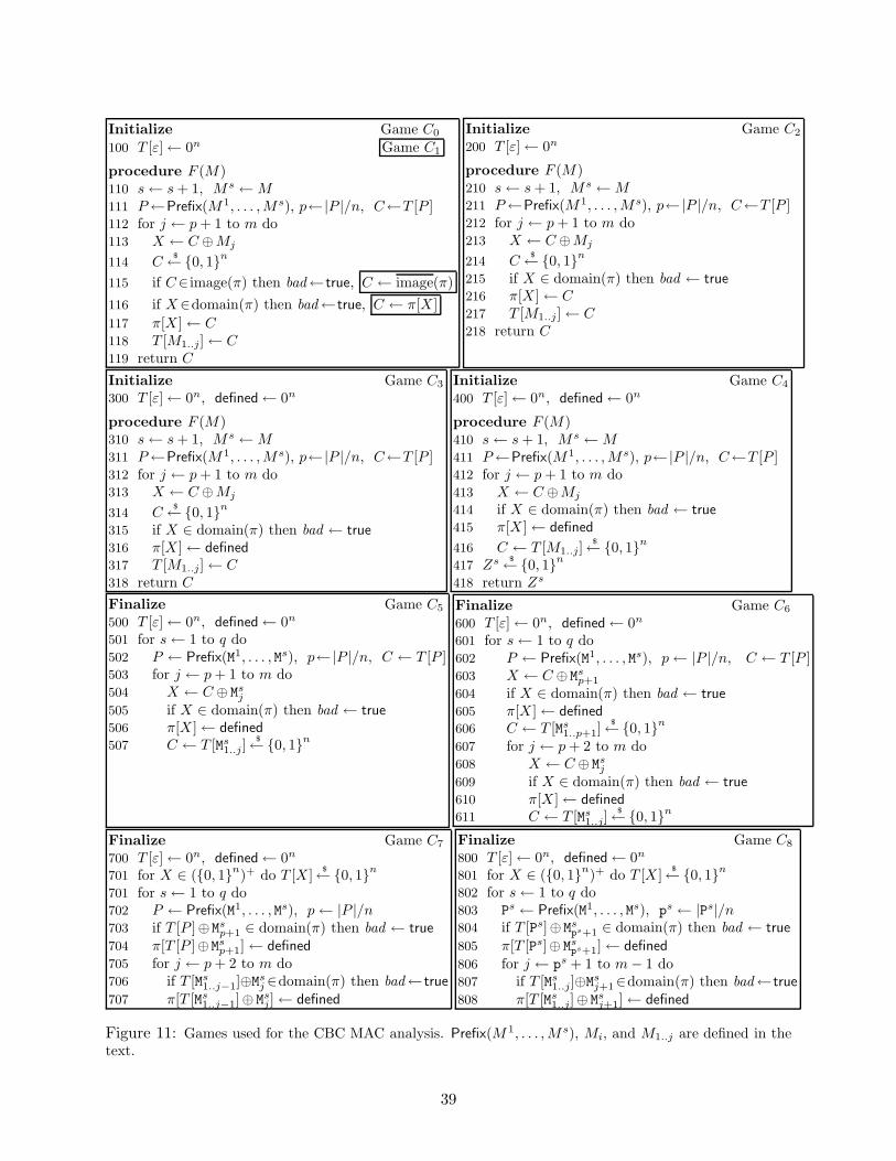
Initialize Game C0

100 T [ε]← 0n Game C1

procedure F (M)110 s← s + 1, M s ←M111 P←Prefix(M1, . . . , Ms), p←|P |/n, C←T [P ]112 for j ← p + 1 to m do113 X ← C ⊕Mj

114 C$←0, 1n

115 if C∈ image(π) then bad← true, C ← image(π)

116 if X∈domain(π) then bad← true, C ← π[X ]

117 π[X ]← C118 T [M1..j]← C119 return C

Initialize Game C2

200 T [ε]← 0n


214 C$← 0, 1n

215 if X ∈ domain(π) then bad ← true

216 π[X ]← C217 T [M1..j ]← C218 return C

Initialize Game C3

300 T [ε]← 0n, defined← 0n


314 C$←0, 1n


316 π[X ]← defined

317 T [M1..j]← C318 return C

Initialize Game C4





416 C ← T [M1..j]$← 0, 1n

417 Zs $←0, 1n

418 return Zs

Finalize Game C5


501 for s← 1 to q do502 P ← Prefix(M1, . . . , Ms), p←|P |/n, C ← T [P ]503 for j ← p + 1 to m do504 X ← C ⊕ Ms

j



507 C ← T [Ms1..j]

$←0, 1n

Finalize Game C6


601 for s← 1 to q do602 P ← Prefix(M1, . . . , Ms), p← |P |/n, C ← T [P ]603 X ← C ⊕Ms

p+1



606 C ← T [Ms1..p+1]

$←0, 1n

607 for j ← p + 2 to m do608 X ← C ⊕Ms

j



611 C ← T [Ms1..j]

$←0, 1n

Finalize Game C7


701 for X ∈ (0, 1n)+ do T [X ]$← 0, 1n

701 for s← 1 to q do702 P ← Prefix(M1, . . . , Ms), p← |P |/n703 if T [P ]⊕Ms

p+1 ∈ domain(π) then bad ← true

704 π[T [P ]⊕Msp+1]← defined

705 for j ← p + 2 to m do706 if T [Ms

1..j−1]⊕Msj ∈domain(π) then bad← true

707 π[T [Ms1..j−1]⊕ Ms

j ]← defined

Finalize Game C8


801 for X ∈ (0, 1n)+ do T [X ]$

← 0, 1n

802 for s← 1 to q do803 Ps ← Prefix(M1, . . . , Ms), ps ← |Ps|/n804 if T [Ps]⊕Ms

ps+1 ∈ domain(π) then bad ← true

805 π[T [Ps]⊕ Msps+1]← defined

806 for j ← ps + 1 to m− 1 do807 if T [Ms

1..j]⊕Msj+1∈domain(π) then bad← true

808 π[T [Ms1..j]⊕ Ms

j+1]← defined

Figure 11: Games used for the CBC MAC analysis. Prefix(M 1, . . . , Ms), Mi, and M1..j are defined in thetext.

39

Finalize Game C9

900 T [ε]← 0n

901 for X ∈ (0, 1n)+ do T [X ]$←0, 1n

902 for s← 1 to q do Ps←Prefix(M1, . . . , Ms), ps←|Ps|/n903 bad ←904 T [Ps]⊕ Ms

ps+1 = T [Pr]⊕Mrpr+1 for some 1 ≤ r < s ≤ q, or

905 T [Ps]⊕ Msps+1 = T [Mr

1..i]⊕Mri+1 for some 1 ≤ r < s ≤ q, pr+ 1≤ i ≤ m−1, or

906 T [Ms1..j ]⊕Ms

j+1 = T [Pr]⊕Mrpr+1 for some 1 ≤ r ≤ s ≤ q, ps+1 ≤ j ≤ m−1, or

907 T [Ms1..j ]⊕Ms

j+1 = T [Mr1..i]⊕Mr

i+1 for some 1 ≤ r ≤ s ≤ q, pr+1 ≤ i ≤ m−1, ps+1 ≤ j ≤ m−1, i<j if r=s

Figure 12: Terminal game used in the analysis of the CBC MAC.

Z1, . . . , Zq instead. Since adversary A is deterministic there are corresponding queries M1, . . . , Mq

that it will ask. As these are constants, we need no longer consider the adversary as interactingwith its oracle; in game C5 we “hardwire in” the sequence of queries M1, . . . , Mq (and responsesZ1, . . . , Zq except that these have no influence on the game) that the adversary A would have asked.The “virtual-queries” M1, . . . , Mq still have to be valid: each Ms is an mn-bit string different fromall prior ones. We have that Pr[AC4 sets bad ] ≤ Pr[C5 sets bad ]. B C5 → C6: Game C6 unrollsthe first iteration of the loop at lines 503–507. This transformation is conservative. B C6 → C7:Game C7 is a rewriting of game C6 that omits mention of the variables C and X, directly usingvalues from the T -table instead, these values now being chosen at the beginning of the game. Thechange is conservative. BC7 → C8: Game C8 re-indexes the for loop at line 705–707. The changeis conservative. BC8 → C9: Game C9 restructures the setting of bad inside the loop at 802–808 toset bad in a single statement. Points were put into the domain of π at lines 805 and 808 and wechecked if any of these points coincide with specified other points at lines 804 and 807. Runningthrough the four possible types of collisions gives rise to the tests at lines 904–907. The change isconservative.

At this point we have only to bound Pr[C9 sets bad ]. We do this using the sum bound and a caseanalysis. Fix a line number among 904, 905, 906, and 907, and fix a corresponding r, i, s, j asspecified on that line. We will show that the probability that the indicated equation holds is atmost 2−n and so, adding the loss incurred in transitioning from From this we can conclude thatPr[C9 sets bad ] ≤ 0.5m2q2 because the total number of equations under consideration is less than0.5m2q2. To see that this is the total number of equations note that we can name a candidateequation by choosing a pair of points (r, i), (q, j) ∈ [1 .. q]× [0 .. m−1] and then rejecting this pairif (r, i) does not proceed (s, j) in lexicographic order. Adding in the 0.5m2q2 term we lost in goingfrom game C0 to game C2, we will be done. The case analysis follows.

Line 904. We first bound Pr[T [Pr]⊕ Mrpr+1 = T [Ps]⊕ Ms

ps+1]. If Pr = Ps = ε then Pr[T [Pr]⊕ Mrpr+1 =

T [Ps]⊕ Msps+1] = Pr[Mr

1 = Ms1] = 0 because Mr and Ms, having only ε as a common block prefix, must

differ in their first blocks. If Pr = ε but Ps 6= ε then Pr[T [Pr]⊕ Mrpr+1 = T [Ps]⊕ Ms

ps+1] = Pr[Mr1 =

T [Ps]⊕ Msps+1] = 2−n since the probability expression involves the single random variable T [Ps] that

is uniformly distributed in 0, 1n. If Pr 6= ε and Ps = ε the same reasoning applies. If Pr 6= ε andPs 6= ε then Pr[T [Pr]⊕ Mr

pr+1 = T [Ps]⊕ Msps+1] = 2−n unless Pr = Ps, so assume that to be the case.

Then Pr[T [Pr]⊕ Mrpr+1 = T [Ps]⊕ Ms

ps+1] = Pr[Mrpr+1 = Ms

ps+1] = 0 because Pr = Ps is the longestblock prefix that coincides in Mr and Ms.

Line 905. We want to bound Pr[T [Ps]⊕ Msps+1 = T [Mr

1..i]⊕ Mri+1]. If Ps = ε then Pr[T [Ps]⊕ Ms

ps+1 =T [Mr

1..i]⊕ Mri+1] = Pr[Ms

ps+1 = T [Mr1..i]⊕ Mr

i+1] = 2−n because it involves a single random value T [Mr1..i].

So assume that Ps 6= ε. Then Pr[T [Ps]⊕ Msps+1 = T [Mr

1..i]⊕ Mri+1] = 2−n unless Ps = Mr

1..i in which

40

case we are looking at Pr[Msps+1 = Mr

ps+1]. But this is 0 because Ps = Mr1..i means that the longest

prefix that Ms shares with Mr is Ps and so Msps+1 6= Mr

ps+1.

Line 906. We must bound Pr[T [Pr]⊕ Mrpr+1 = T [Ms

1..j]⊕ Msj+1]. It is at most by 2−n as above.

Line 907. What is Pr[T [Ms1..j]⊕ Ms

j+1 = T [Mr1..i]⊕ Mr

i+1]. It is 2−n unless i = j and Ms1..j = Mr

1..i. Inthat case ps ≥ j and pr ≥ i, contradicting the allowed values for i and j at line 907. This completesthe proof.

G A Game-Based Proof for OAEP

Background. We recall the needed background for the asymmetric encryption scheme OAEP [8].A trapdoor-permutation generator with associated security parameter k is a randomized algo-rithm F that returns a pair (f, f−1) where f : 0, 1k → 0, 1k is (the encoding of) a permutationand f−1 is (the encoding of) its inverse. Let

AdvowfF (I) = Pr[(f, f−1)

$

←F ; x$

←0, 1k : I(f, f(x)) = x]

be the advantage of adversary I in inverting F . Let ρ < k be an integer. The key-generationalgorithm of asymmetric encryption scheme OAEPρ[F ] is simply F , meaning it returns f as thepublic key and f−1 as the secret key. The encryption and decryption algorithms have oraclesG : 0, 1ρ → 0, 1k−ρ and H : 0, 1k−ρ → 0, 1ρ and work as follows (for the basic, no-authenticity scheme):

algorithm EG,Hf (M) /* M ∈ 0, 1k−ρ */

R$

←0, 1ρ

S ← G(R)⊕M, T ← H(S)⊕RY ← f(S ‖ T )return Y

algorithm DG,Hf−1 (Y ) /* Y ∈ 0, 1k */

X ← f−1(Y )S ← X[1 .. k − ρ], T ← X[k −ρ+1 .. k]R← H(S)⊕ T, M ← G(R)⊕Sreturn M

Security of an asymmetric encryption scheme AE = (F , E ,D) is defined via the following game. Keys(f, f−1) are chosen by running F , and a bit b is chosen at random. Adversary A is given input fand a left-or-right oracle LR(·, · ) which on input a pair M0,M1 of equal-length messages computes

Y$

←Ef (Mb) and returns Y . The output of adversary is a bit b′ and Advind-cpaAE

(A) = 2Pr[b′ = b]−1.

Theorem 15 [IND-CPA security of OAEP] Let F be a trapdoor permutation generator with as-sociated security parameter k, and let ρ < k be an integer. Let A be an adversary with runningtime tA, making at most qG queries to its G oracle, qH to its H oracle, and exactly one query toits left-or-right oracle. Then there is an adversary I with running time tI such that

AdvowfF (I) ≥

1

2Advind-cpa

OAEPρ[F ](A)−

2qG

2ρ−

qH

2k−ρand tI ≤ tA + c qGqH tF

where tF is the time for one computation of a function output by F and c is an absolute constantdepending only on details of the model of computation.

Proof: The proof is based on games shown in Figures 13–15. For these games regard F , k, and ρas fixed; they are hardwired into the games. We have striven to makes steps between adjacentgames small at the cost of a somewhat longer game chain.

For the analysis let pi = Pr[

PAi ⇒ true

]

for 0 ≤ i ≤ 5 (the Finalize procedure of these gamesoutputs a boolean). B Game P0 perfectly mimics the game defining the security of OAEPρ[F ].

41

procedure LR(M0, M1) Game P0

000 R∗ $←0, 1ρ 001 GR∗ $

←0, 1k−ρ002 if G[R∗] then bad ← true, GR∗ ← G[R∗]

003 S∗ ← GR∗⊕Mb 004 HS ∗ $←0, 1ρ 005 if H [S∗] then bad ← true, HS ∗ ← H [S∗]

006 T ∗ ← R∗⊕HS∗ 007 return Y ∗ ← f(S∗ ‖ T ∗)

procedure G(R) procedure H(S)010 if R = R∗ then return G[R∗]← GR∗ 020 if S = S∗ then return H [S∗]← HS∗

011 return G[R]$← 0, 1k−ρ

021 return H [S]$← 0, 1ρ


100 R∗ $←0, 1ρ 101 GR∗ $

←0, 1k−ρ102 S∗ ← GR∗⊕Mb 103 HS ∗ $

← 0, 1ρ

104 T ∗ ← R∗⊕HS∗ 105 return Y ∗ ← f(S∗ ‖ T ∗)

procedure G(R) procedure H(S)110 if R = R∗ then return G[R∗]← GR∗ 120 if S = S∗ then return H [S∗]← HS∗


121 return H [S]$← 0, 1ρ


200 R∗ $←0, 1ρ 201 GR∗ $

←0, 1k−ρ202 S∗ ← GR∗⊕Mb 203 HS ∗ $

← 0, 1ρ

204 T ∗ ← R∗⊕HS∗ 205 return Y ∗ ← f(S∗ ‖ T ∗)

procedure G(R) procedure H(S)210 if R = R∗ then bad ← true, return G[R∗]← GR∗ 220 if S = S∗ then return H [S∗]← HS∗


221 return H [S]$← 0, 1ρ


300 R∗ $←0, 1ρ 301 GR∗ $

←0, 1k−ρ302 S∗ ← GR∗⊕Mb 303 HS ∗ $

← 0, 1ρ

304 T ∗ ← R∗⊕HS∗ 305 return Y ∗ ← f(S∗ ‖ T ∗)

procedure G(R) procedure H(S)310 if R = R∗ then bad ← true 320 if S = S∗ then return H [S∗]← HS∗


321 return H [S]$← 0, 1ρ


400 R∗ $←0, 1ρ 401 S∗ $

←0, 1k−ρ402 HS ∗ $

← 0, 1ρ 403 T ∗ ← R∗⊕HS∗

404 return Y ∗ ← f(S∗ ‖ T ∗)

procedure G(R) procedure H(S)410 if R = R∗ then bad ← true 420 if S = S∗ then return H [S∗]← HS∗


421 return H [S]$← 0, 1ρ


500 R∗ $←0, 1ρ 501 S∗ $

←0, 1k−ρ502 HS ∗ $

← 0, 1ρ 503 T ∗ ← R∗⊕HS∗

504 return Y ∗ ← f(S∗ ‖ T ∗)

procedure G(R) procedure H(S)510 if H [S∗] and R = R∗ then bad ← true 520 if S = S∗ then return H [S∗]← HS∗

511 if ¬H [S∗] and R = R∗ then bad ← true 521 return H [S]$←0, 1ρ


Figure 13: Games used in the analysis of OAEP. Procedure Initialize is the same in all of these games:

(f, f−1)$←F(k), b

$← 0, 1, return f . Procedure Finalize(out) is also the same: return (out = b).

42

procedure LR(M0, M1) Game Q0

000 R∗ $

←0, 1ρ 001 S∗ $

←0, 1k−ρ002 HS ∗ $

← 0, 1ρ 003 T ∗ ← R∗⊕HS∗

004 return Y ∗ ← f(S∗ ‖ T ∗)



021 return H [S]$← 0, 1ρ


100 R∗ $←0, 1ρ 101 S∗ $

←0, 1k−ρ102 T ∗ $

←0, 1ρ 103 HS ∗ ← R∗⊕T ∗

104 return Y ∗ ← f(S∗ ‖ T ∗)



121 return H [S]$← 0, 1ρ


200 S∗ $←0, 1k−ρ

201 T ∗ $←0, 1ρ 202 R∗ $

← 0, 1ρ 203 return Y ∗ ← f(S∗ ‖ T ∗)

procedure G(R) procedure H(S)210 if H [S∗] and R = R∗ then bad ← true 220 if S = S∗ then return H [S∗]← R∗⊕T ∗


221 return H [S]$← 0, 1ρ


300 S∗ $← 0, 1k−ρ

301 T ∗ $←0, 1ρ 302 return Y ∗ ← f(S∗ ‖ T ∗)

procedure G(R) procedure H(S)

310 if H [S∗] and R = R∗ then bad ← true 320 if S = S∗ then R∗ $←0, 1ρ, return H [S∗]←R∗⊕T ∗

311 return G[R]$←0, 1k−ρ

321 return H [S]$←0, 1ρ


400 S∗ $

←0, 1k−ρ401 T ∗ $

←0, 1ρ 402 return Y ∗ ← f(S∗ ‖ T ∗)


410 if H [S∗] and R = R∗ then bad ← true 420 H [S]$← 0, 1ρ


421 if S = S∗ then R∗ ← H [S∗]⊕T ∗

422 return H [S]


500 S∗ $←0, 1k−ρ

501 T ∗ $←0, 1ρ 502 return Y ∗ ← f(S∗ ‖ T ∗)


510 if R = H [S∗]⊕T ∗ then bad ← true 520 return H [S]$← 0, 1ρ



600 S∗ $←0, 1k−ρ

601 T ∗ $←0, 1ρ 602 return Y ∗ ← f(S∗ ‖ T ∗)


610 if ∃ S s.t. f(S ‖ T ∗) = Y ∗ and R = H [S]⊕T ∗ then bad ← true 620 return H [S]$← 0, 1ρ



700 return Y ∗ $← 0, 1k


710 if ∃ S s.t. f(S ‖H [S]⊕R) = Y ∗ then bad ← true 720 return H [S]$←0, 1ρ


Figure 14: Games used in the analysis of OAEP, continued. Initialize and Finalize are as before.43


000 R∗ $←0, 1ρ 001 S∗ $

←0, 1k−ρ002 HS ∗ $

← 0, 1ρ 003 T ∗ ← R∗⊕HS∗

004 return Y ∗ ← f(S∗ ‖ T ∗)

procedure G(R) procedure H(S)010 if ¬H [S∗] and R = R∗ then bad ← true 020 if S = S∗ then return H [S∗]← HS∗


021 return H [S]$←0, 1ρ


100 R∗ $←0, 1ρ 101 S∗ $

←0, 1k−ρ102 HS ∗ $

← 0, 1ρ 103 T ∗ ← R∗⊕HS∗

104 return Y ∗ ← f(S∗ ‖ T ∗)


110 if ¬H [S∗] and R = R∗ then bad ← true 120 return H [S]$←0, 1ρ



200 R∗ $←0, 1ρ 201 S∗ $

← 0, 1k−ρ202 T ∗ $

←0, 1k 203 return Y ∗ ← f(S∗ ‖ T ∗)


210 if R = R∗ then bad ← true 220 return H [S]$

←0, 1ρ


procedure LR(M0, M1) Procedures of Inverter I900 return Y ∗


910 if ∃ S s.t. f(S ‖H [S]⊕R) = Y ∗ then 920 return H [S]$←0, 1ρ

bad ← true, S∗ ‖ T ∗ ← S ‖H [S]⊕R


Figure 15: Top: Games used in the analysis of OAEP, continued. Procedures Initialize and Finalize are asbefore. Bottom: The inverting algorithm I , likewise with an identical Initialize procedure.

Thus

0.5 + 0.5Advind-cpaOAEP

ρ[F ](A) = p0 = p1 + (p0 − p1) ≤ p1 + Pr[P A0 sets bad ] ,

the last step by the Fundamental Lemma. Since game P0 chooses R∗, S∗ at random, Pr[P A0 sets bad ] ≤

qG/2ρ + qH/2k−ρ. BGame P2 differs from game P1 only in the setting of bad , so p1 = p2, and usingthe Fundamental Lemma again we have

p1 = p2 = p3 + (p2 − p3) ≤ p3 + Pr[P A3 sets bad ] .

B In game P4 the string GR∗ is chosen but not referred to in responding to any oracle queriesof the adversary. Thus P4 is a conservative replacement for P3, p3 = p4, and Pr[P A

3 sets bad ] =Pr[P A

4 sets bad ]. However, the bit b is not used in P4, and hence p4 = 1/2. In summary

p3 + Pr[P A3 sets bad ] = p4 + Pr[P A

4 sets bad ] = 1/2 + Pr[P A4 sets bad ] .

Putting all this together we have

0.5Advind-cpaOAEP

ρ[F ](A)−qG

2ρ−

qH

2k−ρ≤ Pr[P A

4 sets bad ] . (24)

We proceed to upper bound the right-hand-side of the above. We have

Pr[P A4 sets bad ] ≤ Pr[P A

5 sets bad ] ≤ Pr[QA0 sets bad ]+Pr[QA

0 sets bad ] ≤ Pr[QA0 sets bad ]+qG/2ρ .

44

Above, we have split the analysis of game P5 into the analysis of games Q0 and Q0, the former beingaccomplished by the game chain at Figure 14 and the latter by the game chain of Figure 15. Thesecond term is readily shown to be at most qG/2ρ by way of the game chain at Figure 15. Goingback to the analysis of game Q0 in Figure 14, we have a series of conservative changes, giving Q1,Q2, Q3, Q4, Q5 leading to

Pr[QA0 sets bad ] = Pr[QA

5 sets bad ] ≤ Pr[QA6 sets bad ] = Pr[QA

7 sets bad ] .

To conclude the proof we design I so that

Pr[QA7 sets bad ] ≤ Advowf

F (I) . (25)

On input f, Y ∗, inverter I runs A on input public key f , responding to its oracle queries via theprocedures specified in the last box in Figure 15. When A halts, inverter I returns S ∗ ‖ T ∗ if thishas been defined. By comparison with game Q7 we see that (25) is true, completing the proof.

45

professor.unisinos.brprofessor.unisinos.br/linds/teoinfo/bellare06codebased.pdfCode-Based...

Documents

Transcript of professor.unisinos.brprofessor.unisinos.br/linds/teoinfo/bellare06codebased.pdfCode-Based...