Gambling for Redemption and Self-Fulfilling Debt Crises

Juan Carlos Conesa Stony Brook University

Timothy J. Kehoe University of Minnesota

and Federal Reserve Bank of Minneapolis

April 2014

2

Jumps in spreads on yields on bonds of PIIGS governments (over yields on German bonds)

0

2

4

6

8

10

12

14

16

2007 2008 2009 2010 2011 2012 2013 2014

perc

ent p

er y

ear

GreecePortugal

Germany

Spain

Ireland

Italy

Yields on 10-year government bonds

3

Theory of self-fulfilling debt crises (Cole-Kehoe) Spreads reflect probabilities of crises For low enough levels of debt, no crisis is possible For high enough levels of debt, default For intermediate levels of debt (crisis zone) optimal policy is to run down debt

4

…but PIIGS ran up debt.

0

20

40

60

80

100

120

140

160

2007 2008 2009 2010 2011 2012

perc

ent o

f 200

7 G

DP

Greece

Italy

Portugal

Germany

Spain

Ireland

Government debt

5

What is missing in Cole-Kehoe?

6

Severe recession in PIIGS, still ongoing

80

85

90

95

100

105

110

2005 2006 2007 2008 2009 2010 2011 2012

GD

P pe

r wor

king

age

per

son

(200

7 =

100)

Greece

Italy

Portugal

Germany

Spain

Ireland

Real GDP

7

…government revenues also depressed.

80

85

90

95

100

105

110

2005 2006 2007 2008 2009 2010 2011 2012

reve

nue

per w

orki

ng a

ge p

erso

n (2

007

= 10

0)

Greece

Italy

Portugal

Germany

Spain

Ireland

Real government revenues

8

This paper Extends Cole-Kehoe to stochastic output. Standard consumption smoothing argument in an incomplete markets model (as in Aiyagari, Huggett, Chaterjee et al, Arellano, Aguiar-Gopinath) can imply running up debt. When running up debt is optimal, we call it “gambling for redemption.” Use model to evaluate impact of Troika (EU-ECB-IMF) policy, compare with the Clinton (1995) bailout of Mexico.

9

Main mechanism of our theory Model characterizes two forces in opposite directions:

1. Run down debt (as in Cole-Kehoe)

2. Run up debt (consumption smoothing) Which one dominates depends on parameter values and Troika policies.

10

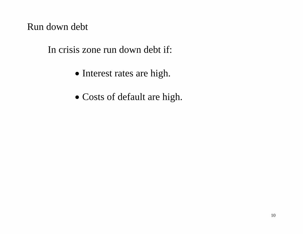
Run down debt In crisis zone run down debt if:

Interest rates are high.

Costs of default are high.

11

Run up debt In recession run up debt if:

Interest rates are low.

Costs of default are low.

Recession is severe.

Probability of recovery is high.

12

General model

Agents:

Government

International bankers, continuum [0,1]

Consumers, passive (no private capital)

Third party in policy experiments

13

General model

State of the economy: 1( , , , )s B a z

B: government debt

a : private sector, 1a normal, 0a recession

1z : previous default 1 1z no, 1 0z yes

: realization of sunspot

GDP: 1 1( , ) a zy a z A Z y

1 0A , 1 0Z parameters.

14

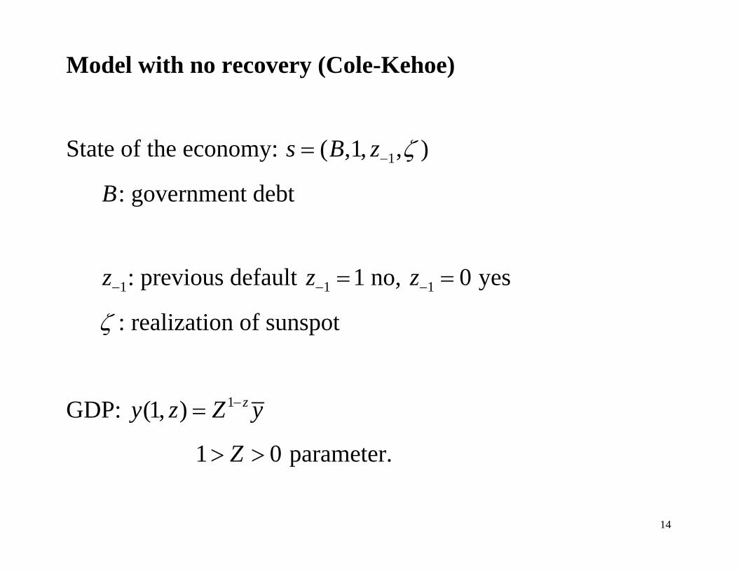
Model with no recovery (Cole-Kehoe)

State of the economy: 1( ,1, , )s B z

B: government debt

1z : previous default 1 1z no, 1 0z yes

: realization of sunspot

GDP: 1(1, ) zy z Z y

1 0Z parameter.

15

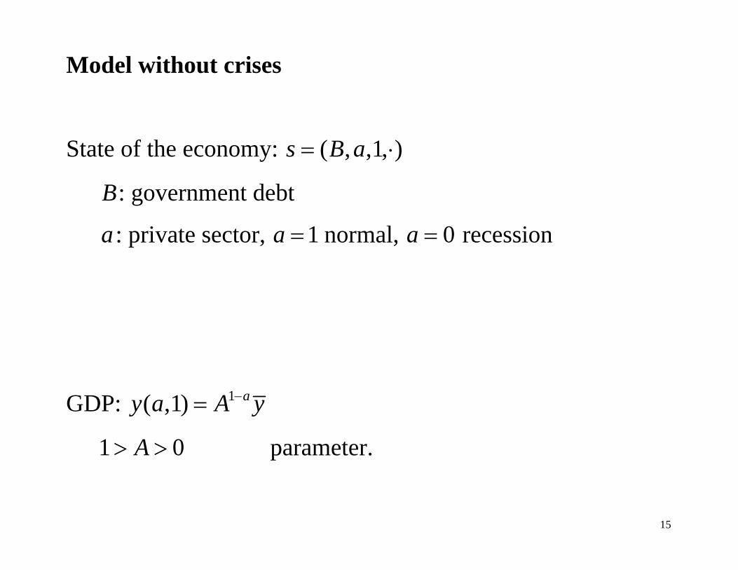
Model without crises

State of the economy: ( , ,1, )s B a

B: government debt

a : private sector, 1a normal, 0a recession

GDP: 1( ,1) ay a A y

1 0A parameter.

16

General model

Before period 0, 1a , 1z .

In 0t , 0 0a unexpectedly, GDP drops from y to Ay y .

In 1,2,...t , ta becomes 1 with probability p .

1 A is severity of recession. Once 1ta , it is 1 forever.

1 Z is default penalty. Once 0tz , it is 0 forever.

17

A possible time path for GDP

t recession default recovery

y

y

Ay AZy

Zy

18

Sunspot

Coordination device for international bankers’ expectations.

[0,1]t U

tB outside crisis zone: if t is irrelevant

tB inside crisis zone: if 1t bankers expect a crisis (

arbitrary)

19

Government’s problem

Depends on timing, equilibrium conditions, to be described.

Government tax revenue is ( , )y a z , tax rate is fixed.

Choose , , ',c g B z to solve:

( ) max ( , ) ( ')V s u c g EV s

s.t. (1 ) ( , )c y a z

( , ) ( ', ) 'g zB y a z q B s B

0z if 1 0z .

20

International bankers

Continuum [0,1] of risk-neutral agents with deep pockets

First order condition and perfect foresight condition:

( ', ) ( ', ', ( ', '))q B s Ez B s q B s .

bond price = risk-free price × probability of repayment

21

Timing

ta , t realized, 1( , , , )t t t t ts B a z

government offers 1tB

bankers choose to buy 1tB or not, tq determined

government chooses tz , which determines ty , tc , and tg

22

Notes

Time-consistency problem: when offering 1tB for sale,

government cannot commit to repay tB

Perfect foresight: bankers do not lend if they know the

government will default.

Bond price depends on 1tB ; crisis depends on tB .

23

Recursive equilibrium

Value function for government ( )V s and policy functions

'( )B s and ( ', , )z B s q and ( ', , )g B s q ,

and a bond price function ( ', )q B s

such that:

24

1. Beginning of period: Given ( ', , )z B s q , ( ', , )g B s q , ( ', )q B s

government chooses 'B to solve:

( ) max ( , ) ( ')V s u c g EV s

s.t. (1 ) ( , ( ', , ( ', ))c y a z B s q B s

( ', , ( ', )) ( ', , ( ', )) ( , ) ( ', ) 'g B s q B s z B s q B s B y a z q B s B

2. Bond market equilibrium:

( '( ), ) ( '( '), ', ( '( '), '))q B s s Ez B s s q B s s .

25

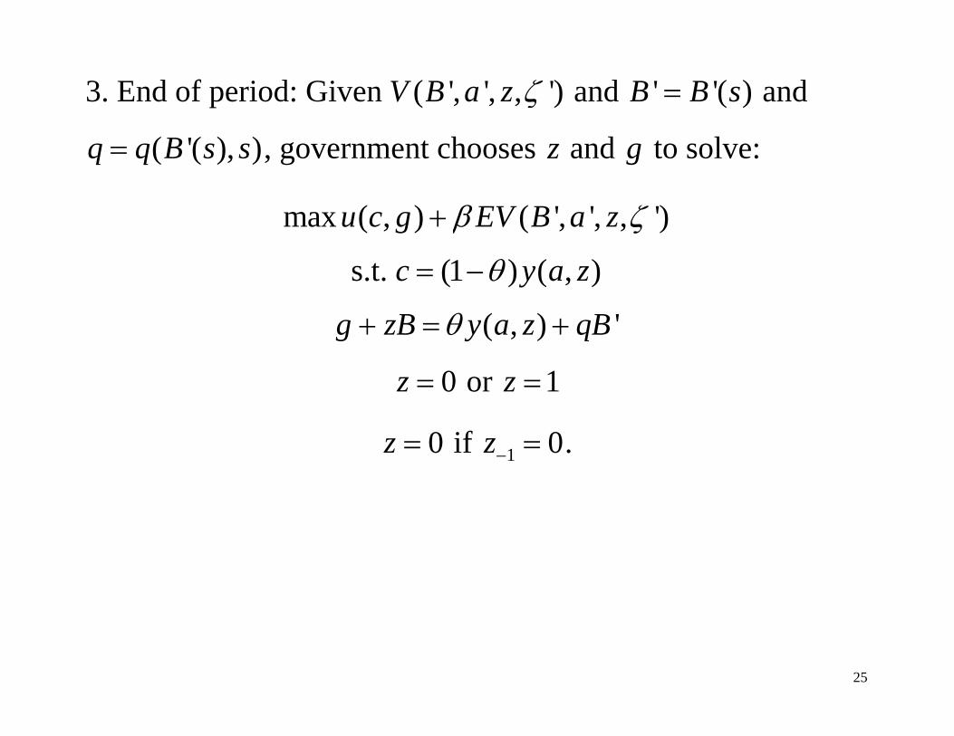
3. End of period: Given ( ', ', , ')V B a z and ' '( )B B s and

( '( ), )q q B s s , government chooses z and g to solve:

max ( , ) ( ', ', , ')u c g EV B a z

s.t. (1 ) ( , )c y a z

( , ) 'g zB y a z qB

0z or 1z

0z if 1 0z .

26

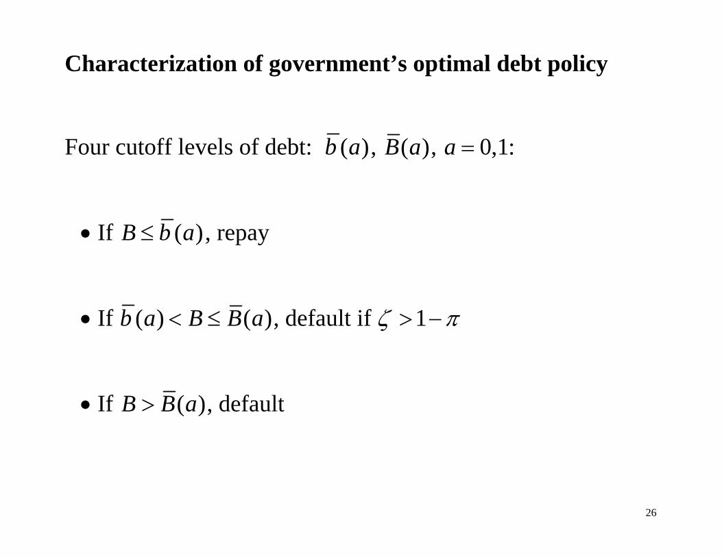
Characterization of government’s optimal debt policy

Four cutoff levels of debt: ( )b a , ( )B a , 0,1a :

If ( )B b a , repay

If ( ) ( )b a B B a , default if 1

If ( )B B a , default

27

We are interested in parameter values for which

(0) (1)b b , (0) (0)b B , (1) (1)b B , and (0) (1)B B .

(1)b , (0)B ?

Most interesting case:

(0) (1) (0) (1)b b B B .

Other cases (catastrophic recessions):

(0) (0) (1) (1)b B b B

(0) (1) (0) (1)b b B B .

28

Characterization of equilibrium prices

After default bankers do not lend: ( ', ( , ,0, )) 0q B B a .

During a crisis bankers do not lend: If ( )B b a and

1 , ( ', ( , ,1, )) 0q B B a

Otherwise, q depends only on 'B .

29

In normal times (as in Cole-Kehoe):

if ' (1)( ', ( ,1,1, )) (1 ) if (1) ' (1)

0 if (1) '

B bq B B b B B

B B

In a recession (for the most interesting case):

if ' (0)

(1 )(1 ) if (0) ' (1)

( ', ( ,0,1, )) (1 ) if (1) ' (0)(1 ) if (0) ' (1)

0

B bp p b B b

q B B b B Bp B B B

if (1) 'B B

30

Bond prices as function of debt and a

(0)b (1)b (0)B (1)B 'B

( ', )q B a

( ',0)q B

( ',1)q B

31

Characterization of optimal debt policy Two special cases with analytical results: 0p (no gambling for redemption) 0 (no crises)

General model with numerical experiments: ( )V s has kinks and '( )B s is discontinuous because of

discontinuity of ( ', )q B s . ( )V s is discontinuous because government cannot commit

not to default. .

32

Self-fulfilling liquidity crises, no gambling

0p , also limiting case where 0a and 0p : Replace y with Ay .

Cole-Kehoe without private capital.

33

Start by assuming that 0 .

When 1( , , , ) ( ,1,1, )s B a z B ,

((1 ) , (1 ) )( ,1,1, )1

u y y BV B

.

When default has occurred, 1( , , , ) ( ,1,0, )s B a z B ,

((1 ) , )( ,1,0, )1

u Zy ZyV B

.

34

(1)b :

Utility of repaying even if bankers do not lend:

((1 ) , )((1 ) , )1

u y yu y y B

Utility of defaulting if bankers do not lend:

((1 ) , )1

u Zy Zy

.

(1)b is determined by

((1 ) , ) ((1 ) , )((1 ) , (1))1 1

u y y u Zy Zyu y y b

35

Determination of (1)B requires optimal policy.

If 0 (1)B b and the government decides to reduce B to (1)b

in T periods, 1,2,...,T . First-order conditions imply

0( )Ttg g B .

10 0

1 (1 )( ) ( (1 )) (1)1 ( (1 ))

T TTg B y B b

.

0 0 0( ) lim ( ) (1 (1 ))TTg B g B y B .

36

Compute 0( )TV B :

0 0

1

2

1 ( (1 ))( ) ((1 ) , ( ))1 (1 )

1 ( (1 )) ((1 ) , ) 1 (1 ) 1

((1 ) , ) ( (1 ))1

TT T

T

T

V B u y g B

u Zy Zy

u y y

37

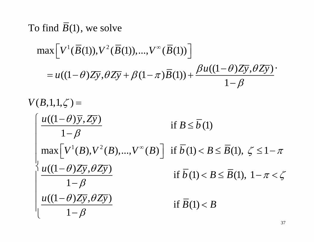
To find (1)B , we solve

1 2max ( (1)), ( (1)),..., ( (1))

((1 ) , ) ((1 ) , (1 ) (1))1

V B V B V B

u Zy Zyu Zy Zy B

.

1 2

( ,1,1, )((1 ) , ) if (1)

1

max ( ), ( ),..., ( ) if (1) (1), 1 ((1 ) , ) if (1) (1), 1

1((1 ) , )

1

V Bu y Zy B b

V B V B V B b B B

u Zy Zy b B B

u Zy Zy

if (1)B B

38

Equilibrium with self-fulfilling crises, no crises

(1)B

(1)b

0 1 2 3 4 t

tB always default

crisis zone

0q

(1 )q

q

39

Consumption smoothing without self-fulfilling crises

0a and 0 .

Private sector is in a recession and faces the possibility p of

recovering in every period.

40

Uncertainty tree with recession path highlighted

1a

1a

1a

1a

1a

1a 0a

0a

0a

41

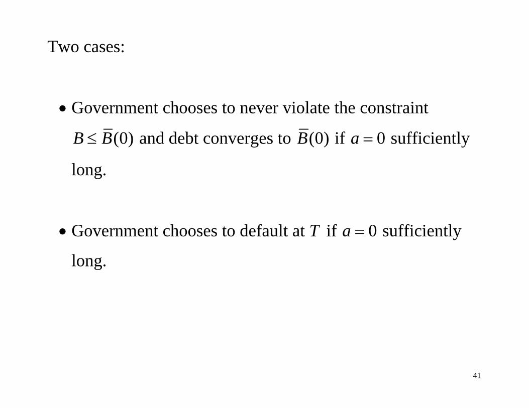
Two cases:

Government chooses to never violate the constraint

(0)B B and debt converges to (0)B if 0a sufficiently

long.

Government chooses to default at T if 0a sufficiently

long.

42

Equilibrium with no default

(1)B

(0)B

0 1 2 3 4 t

tB always default

default unless 1a

0q

q p

q

43

Equilibrium with eventual default

(1)B

(0)B

0 1 2 3 4 t

tB always default

default unless 1a

0q

q p

q

44

Quantitative analysis in a numerical model

( , ) log( ) log( )u c g c g g

Parameter ValueA 0.90 Z 0.95 p 0.20 0.98 0.03 0.25 0.40 y 100 g 25

45

We work first with one-year bonds. We then extend model to multi-year bonds.

46

Results: The benchmark economy in normal times

0

10

20

30

40

50

60

70

80

0 10 20 30 40 50 60 70 80

b (1)B (1)

47

Then, a recession hits…

0

10

20

30

40

50

60

70

80

0 10 20 30 40 50 60 70 80

b (1)b (0) B (1)B (0)

48

Maturity of debt in 2011

Weighted average years until maturity

Germany 6.4Greece 15.4Ireland 4.5Italy 6.5Portugal 5.1Spain 5.9

Think of results in terms of debt needing refinancing every year — say one-sixth, as in Spain.

49

The extended model The government’s problem is to choose , , ',c g B z to solve

( ) max ( , ) ( ')V s u c g EV sb= +

s.t. (1 ) ( , )c y a zq= -

( )( , ) ( ', ) ' (1 )g z B y a z q B s B Bd q d+ = + - -

0z if 1 0z .

Here [ ]0,1d Î is the fraction of the stock of debt due every period. Debt is memoryless, as in Hatchondo-Martinez, Chaterjee-Eyigungor.

50

Prices are also adjusted

In the benchmark case (0) (1) (0) (1)b b B B< < < :

[ ]( )[ ]

[ ][ ]

(1 ) ' if ' (0)

(1 )(1 ) (1 ) ' if (0) ' (1)

( ', ) (1 ) (1 ) ' if (1) ' (0)

(1 ) (1 ) '

Eq B b

p p Eq b B b

q B s Eq b B B

p Eq

b d d

b p d d

b p d d

b p d d

+ - £

+ - - + - < £

= - + - < £

- + - if (0) ' (1)

0 if (1) '

B B B

B B

ìïïïïïïïïíïïï < £ïïïï <ïî

where ' ( '( ', ), ')Eq Eq B B s s .

51

Benchmark is 1d=

0

20

40

60

80

100

120

0 20 40 60 80 100 120

b (0) b (1) B (0)B (1)

52

With 0.5d=

0

20

40

60

80

100

120

0 20 40 60 80 100 120

b (0) b (1)

B (0) B (1)

53

With 0.25d=

0

20

40

60

80

100

120

0 20 40 60 80 100 120

b (0) b (1)

B (0) B (1)

54

With 0.167d=

0

20

40

60

80

100

120

0 20 40 60 80 100 120

b (0) b (1)

B (0) B (1)

55

As d becomes smaller:

The thresholds shift to the right and get closer together. Gambling for redemption also for low (but vulnerable) levels of debt.

In the limit, 0d= (consuls) the lower and upper thresholds coincide and huge levels of debt can be sustained (larger than 700 percent GDP).

56

Extensions:

Keynesian features Panglossian borrowers á la Krugman (1998) Time varying risk premia

57

Keynesian features Government expenditures are close substitutes for private consumption expenditures:

( , ) log( )u c g c g c g . Probability of recovery ( )p g varies positively with government expenditures:

'( ) 0p g .

58

Keynesian features Government expenditures are close substitutes for private consumption expenditures:

( , ) log( )u c g c g c g . Probability of recovery ( )p g varies positively with government expenditures:

'( ) 0p g . Keynesian features make gambling for redemption more attractive!

59

Panglossian borrowers Krugman (1998), Cohen and Villemot (2010) The government is overly optimistic about the probability of a recovery:

gp p where p is the probability that international lenders assign to a recovery.

60

Suppose that

( ', ) (1 )(1 )q B s p p or

( ', ) (1 )q B s p . Then holding gp fixed and lowering p results in lower

'( , )B B s . Similarly, holding p fixed and increasing gp results in lower

'( , )B B s .

61

We could also analyze the case where the government is overly optimistic about the probability of a self-fulfilling crisis:

g and obtain similar results. Bottom line: Optimistic governments feel the market charges too much of a premium and hence want to reduce debt. Pessimistic governments (or governments with private information about the low probability of recovery) want to increase debt.

62

Time varying risk premia Two different probabilities of a self-fulfilling crisis, 2 1 , transitions follow a Markov process:

11 12

21 22

.

A country can be repaying its debts when faced with 1 , then make the transition to 2 and be forced to default.

63

Concluding remarks Model provides: Plausible explanation for the observed behavior of PIIGS. Reasonable quantitative predictions for longer maturities.

Why Greece and not Belgium?

64

Concluding remarks Model provides: Plausible explanation for the observed behavior of PIIGS. Reasonable quantitative predictions for longer maturities.

Why Greece and not Belgium? Why the Eurozone and not the United States? What about bailouts and costly reforms?

65

Role of bailouts: Conesa-Kehoe, “Is it too late to bail out the troubled countries in the Eurozone?” Suppose that when a panic occurs, a third party (Troika) offers access to credit at a penalty interest rates and imposes collateral requirements (Bagehot, Clinton) Results: If premium is small, continue gambling

If premium is high enough to discourage gambling, then it is optimal to default instead of accepting the bailout for debt levels higher than around 80 percent GDP.