1

Avoiding qPCR InhibitionProper dilution of RNA isolates is key to

truly relative log-linear quantitative analysis for one-step fluorogenic real-time qPCR

in brief …

J.M. Gallup (eag@iastate.edu)

Dr. Mark Ackermann’s Lab

Department of Veterinary Pathology, Iowa State University

Forms of qPCR Inhibition to be aware of:Based on experimental observations of the dynamics of numerous real-time qPCR reactions, we have been able to label and organize qPCR inhibitory phenomena into five different categories; Types 1-5:

1.) Inhibition of reverse transcriptase (RT) enzyme(s) and/or Taq DNA polymerase(s) by excessive rRNA and possibly tRNA in concentrated RNA samples (sample concentration-related template inhibition),

2.) Method of RNA isolation resulting in the carryover of inhibitory biological components or molecules (sample isolation-related inhibition),

3.) Inhibition arising from the type of tissue or cell that sample RNA has been isolated from (sample-specific inhibition),

4.) Inhibition resulting from interaction of a specific qPCR template with its specific probe and primer(s) (target-specific template inhibition),

5.) Inhibition caused by compounds such as EDTA, GIT, TRIS, glycogen, or any other user-introduced reagents (chemical inhibition)

2

Some qPCR-inhibitory (carryover) biological contaminants are thought to be: hemoglobin, heme, porphyrin, heparin (from peritoneal mast cells), glycogen (>2 mg/mL), polysaccharides, other unknown cell constituents, Ca2+, DNA or RNA concentration, and DNA (possibly RNA) binding proteins, or other proteins (Pfaffl, et.al, Bustin [A-Z of Quantitative PCR] p. 167).

MicroRNA (miRNA) is not thought to be a contributing factor to qPCR inhibition since high thermocylcingtemperatures (94-95°C) most likely disallow the formation of stable RNA-binding RSK complexes which might associate with template RNA (Ambiontechnical services comment).

Type 1 inhibition: inhibition of reverse transcriptase enzymes by rRNA and tRNA is not understood well, but has been noted in Invitrogen product literature (ref: Instruction Manual: SuperScript™ III CellsDirect, cDNA Synthesis System Catalog Nos. 18080-200 and 18080-300, Version A, 14 May 2004, 25-0731, page vi) …Understandably, inhibition Types 2 and 3 will always be a function of one another as method of RNA isolation and tissue or cell type from which the RNA is isolated will always affect one another distinctly. Similarly, inhibition types 1&2, 1&3, 1&4 and 1&5 are all sample-dilution dependent; a lessening of all types of inhibition is expected with increasing sample dilutions … logicallySince our qPCR studies involve the sole use of the TaqMan® (hydrolysis) probe method (which includes the use of sequence-specific forward and reverse primers), we discuss here only observations we have made with this approach using total RNA as template in fluorogenic one-step real-time qPCR … (for all targets we use 1000 nM primers and 150 nM probe concentrations) …

Invitrogen literature

3

In addition to two conventional PCR primers, P1 and P2, which are specific for the target sequence, a third primer, P3 (called the ‘probe’), is designed to bind specifically to a site on the target sequence downstream of the forward primer binding site. The probe is labelled with two fluorophores, a reporter dye (R) is attached at the 5’ end while a quencher dye (D), which has a different emission wavelength to the reporter dye, is attached at its 3’ end. Because the 3’ end is blocked (by the quencher), the probe cannot by itself prime any new DNA synthesis. During the PCR reaction, Taq DNA polymerase synthesizes a new DNA strand primed by the forward primer, and as the enzyme approaches the probe, its 5’ to 3’ exonuclease activity progressively degrades the probe from its 5’ end. The end result is that the nascent DNA strand extends beyond the probe binding site and the reporter and quencher dyes are no longer bound to the same molecule. As the reporter dye is no longer in close proximity to the quencher, the resulting increase in reporter emission intensity becomes easily detectable. This all occurs in “real time” as monitored by the photomultiplier tube(s) in each qPCR instrument.

P1 = Forward Primer

P2 = Reverse Primer

P3 = Fluorogenic TaqMan hydrolysis probe

The TaqMan 5’exonuclease assay

Fluorescing Real-Time qPCR

ProbeReporter Quencher

Primer

Single stranded cDNA

by Charles Brockus

4

Common inhibitory profiles observed during one-step real-time qPCR using Trizol-isolated RNA from tissues and cell culture samples …

One must identify the optimal dilution range for each qPCR target per RNA-isolation method used. This is the range over which a target shows a log linear relationship between Ct and template dilution while also exhibiting a high efficiency of reaction (>80%)

G1 "in-well"start useful stnd curve at 1: 1000 1000

serial 1: 10 10000Efficiency: 99.67% 119.26% (Better E) 100000

Correlation: -1.000 1000000b = 25.175m = -3.3298

Make final manual adjustments of rangesG2 "in-well"start useful stnd curve at 1: 1000 1000

serial 1: 10 10000Efficiency: 100.09% 113.65% (Better E) 100000

Correlation: -1.000 1000000b = 23.798m = -3.3198

chR18S "in-well"start useful stnd curve at 1: 50000 50000

serial 1: 5 250000Efficiency: 103.98% 115.44% (Better E) 1250000

Correlation: -0.999 6250000b = 10.149m = -3.2300

Apparent good Stnd Curve

y = -3.3198x + 23.798R2 = 0.9997

05

101520253035404550

-4 -3.5 -3 -2.5 -2 -1.5 -1 -0.5 0

[log]

Ct

Apparent good Stnd Curve

y = -3.23x + 10.149R2 = 0.9983

05

101520253035404550

-4 -3 -2 -1 0[log]

Ct

Apparent good Stnd Curve

y = -3.3298x + 25.175R2 = 0.9994

05

101520253035404550

-4 -3.5 -3 -2.5 -2 -1.5 -1 -0.5 0

[log]

Ct

OUR GOAL HERE IS TO FIND THE TEMPLATE

DILUTION RANGE (FOR EACH DIFFERENT TARGET)WHICH EXHIBITS LINEARITY

AND HIGH EFFICIENCYWHILE AVOIDING ALL qPCR INHIBITORY PHENOMENA

5

Machine Factors: 0.026 0.02 0.01 0.005 0.002 0.001 0.0002 0.0001 0.00002 0.000002 0.00000021 2 3 4 5 6 7 8 9 10 11 12

A hRSV

B SBD-1

C SP-D

D SP-A

E TTF-1

F ovRPS15

G h18S

HTested Concentrations to see where inhibition lets up for each different target

Initial RNA is already at 1: 10 in well will actually be a 1: 38.46After DNAse treatment: Desired final in-well test dilution 1: 50 Desired final in-well test dilution 1: 10000samples are diluted 1: 10 Desired final in-well test dilution 1: 100 Desired final in-well test dilution 1: 50000And samples, after further Desired final in-well test dilution 1: 200 Desired final in-well test dilution 1: 500000dilutions, are then used in-well Desired final in-well test dilution 1: 500 Desired final in-well test dilution 1: 5000000at a proportion of: Desired final in-well test dilution 1: 1000

7.80 uL sample Desired final in-well test dilution 1: 500030.00 uL well size Given that our Stock I Solution RNA mixture is calculated to be: 48.18545 ng/uL (comprised of 1:10 RNAs)

sample fractio n is thus: 0.26 This Test Plate dilution series thus represents: 12.52822 ng/uL in well9.637091 ng/uL in well4.818545 ng/uL in well2.409273 ng/uL in well0.963709 ng/uL in well

Stock I Range tested 0.481855 ng/uL in well0.096371 ng/uL in well0.048185 ng/uL in well0.009637 ng/uL in well0.000964 ng/uL in well9.64E-05 ng/uL in well

NTC 1:38.46 1:50 1:100 1:200 1:500 1:1000 1:5000 1:10000 1:50000 1:500000 1:5000000

NTC 1:38.46 1:50 1:100 1:200 1:500 1:1000 1:5000 1:10000 1:50000 1:500000 1:5000000

NTC 1:38.46 1:50 1:100 1:200 1:500 1:1000 1:5000 1:10000 1:50000 1:500000 1:5000000

NTC 1:38.46 1:50 1:100 1:200 1:500 1:1000 1:5000 1:10000 1:50000 1:500000 1:5000000

NTC 1:38.46 1:50 1:100 1:200 1:500 1:1000 1:5000 1:10000 1:50000 1:500000 1:5000000

NTC 1:38.46 1:50 1:100 1:200 1:500 1:1000 1:5000 1:10000 1:50000 1:500000 1:5000000

NTC 1:38.46 1:50 1:100 1:200 1:500 1:1000 1:5000 1:10000 1:50000 1:500000 1:5000000

Custom file

EXAMPLE 7-TARGET TEST PLATE SET-UP

Using a standard RNA (containing all your targets of interest), run a test plate, testing variousdilutions of the RNA until it no longer exhibits template or chemical inhibition of each qPCR rxn …Decide where your standard curves should start for each target (e.g. always after the point oftemplate or chemical inhibition for each target) …

FROM YOUR OBSERVATIONS OF THE TEST PLATE RESULTS, DECIDE THE FOLLOWING:(Decide what target needs the most concentrated RNA in order to be found adequately byqPCR. Enter that target and its apparent 1st useful dilution in the yellow area below):List in order of abundance from weakest to strongest (as observed from Cts on your Test Plate)

Enter values of This serves as the 1st point (dilution) in the standard curve for this targetTEST PLATE OBSERVATIONS apparent 1st ng/uL (in-well) that this dilution actually Apparent useful serial dilution

(least abundant target; "limiting" factor) useful dilution 1: corresponds to (info from Sheet 3 used) factor for each Stnd Crve 1:

Target 1 G-1 1000 0.2085 ng/uL in-well 10

Target 2 G-2 1000.00001 0.2085 ng/uL in-well 10

Target 3 ch18S 50000 0.0042 ng/uL in-well 5

Target 4 ? ? #VALUE! ng/uL in-well ?

Target 5 ? ? #VALUE! ng/uL in-well ?Target 6 ? ? #VALUE! ng/uL in-well ?Target 7 ? ? #VALUE! ng/uL in-well ?

G-1 G-2 ch18S1000 1000.00001 5000010000 10000.0001 250000

100000 100000.001 12500001000000 1000000.01 6250000

Or, in final ng/uL (in well values):G-1 G-2 ch18S

0.2085 0.2085 0.00420.0209 0.0209 0.00080.0021 0.0021 0.00020.0002 0.0002 0.0000

To fit within stnd curve: Apparent usefulName Unknown dilution 1: (in-well) These factors are used in

Target 1 G-1 5500 0.03792 ng/uL in-well Sheet 2 (serialdilutionx)Target 2 G-2 5500.000055 0.03792 ng/uL in-well 1.00000001 1.00000001 1.00000001 1 1.00000001Target 3 ch18S 150000 0.00139 ng/uL in-well 27.27272727 27.27272727 27.27272727 27.27273 27.27272727

Have to have at least 3 samples here, and for any

samples that share identical

dilutions, be sure to alter 1 of them

slightly -- i.e. 1:300 and

1:300.000001 etc. -- or else the file will not work

Type into 5700 as factors for Stnd curve relative dilutions:

G-1 G-2 ch18S1 1 1

0.1 0.1 0.20.01 0.01 0.040.001 0.001 0.008

6

(in-well) (in-well) The Final print-out for final sample serial dilutions to get them into the appropriate useful One-Step real-time qPCR ranges without inhibition …1st-sample 1st-sample Sample 1:10 RNA Water epMtn from previous Water 415 uL from previous Water 15 uL

Dilutions incurred Dilutions incurred 1st tier check BoneM1 20.0 uL 4823.79 uL 750 uL 414.67 uL 0.00 uL 0 uL 14.67 uL 385.33 uL 386 uL

Post DNase 1: Since isolation 1: in ng/uL Jej1 1.8 uL 1474.12 uL 750 uL 414.67 uL 0.00 uL 14.67 uL 385.33 uL9314.98 14637.82 0.037915 Crop1 6.0 uL 1427.76 uL 750 uL 414.67 uL 0.00 uL 14.67 uL 385.33 uL

31536.66 49557.61 0.037915 Testes1 2.0 uL 1303.99 uL 750 uL 414.67 uL 0.00 uL 14.67 uL 385.33 uL9190.78 14442.65 0.037915 Lung1 2.0 uL 1267.16 uL 750 uL 414.67 uL 0.00 uL 14.67 uL 385.33 uL

25115.20 39466.74 0.037915 Skin1 2.0 uL 1101.69 uL 750 uL 414.67 uL 0.00 uL 14.67 uL 385.33 uL24406.92 38353.74 0.037915 Spleen1 2.0 uL 1014.76 uL 750 uL 414.67 uL 0.00 uL 14.67 uL 385.33 uL21224.73 33353.14 0.037915 Liver1 1.6 uL 1546.04 uL 750 uL 414.67 uL 0.00 uL 14.67 uL 385.33 uL19553.06 30726.24 0.037915 Kidny1 1.0 uL 1183.85 uL 750 uL 414.67 uL 0.00 uL 14.67 uL 385.33 uL37202.85 58461.62 0.037915 Bursa1 2.0 uL 1140.26 uL 750 uL 414.67 uL 0.00 uL 14.67 uL 385.33 uL45571.23 71611.93 0.037915 Trach1 5.0 uL 1049.29 uL 750 uL 414.67 uL 0.00 uL 14.67 uL 385.33 uL21966.57 34518.89 0.037915 Conj1 4.0 uL 1403.58 uL 750 uL 414.67 uL 0.00 uL 14.67 uL 385.33 uL8109.91 12744.14 0.037915 Tongue1 2.0 uL 1144.63 uL 750 uL 414.67 uL 0.00 uL 14.67 uL 385.33 uL

13534.41 21268.36 0.037915 BoneM2 8.0 uL 1274.60 uL 750 uL 414.67 uL 0.00 uL 14.67 uL 385.33 uL22050.49 34650.76 0.037915 Jej2 2.0 uL 1095.75 uL 750 uL 414.67 uL 0.00 uL 14.67 uL 385.33 uL6166.35 9689.98 0.037915 Crop2 2.0 uL 1051.07 uL 750 uL 414.67 uL 0.00 uL 14.67 uL 385.33 uL

21110.60 33173.79 0.037915 Ovid2 16.0 uL 1402.75 uL 750 uL 414.67 uL 0.00 uL 14.67 uL 385.33 uL20251.27 31823.42 0.037915 Lung2 2.0 uL 1072.54 uL 750 uL 414.67 uL 0.00 uL 14.67 uL 385.33 uL3410.46 5359.29 0.037915 Skin2 10.0 uL 1002.40 uL 750 uL 414.67 uL 0.00 uL 14.67 uL 385.33 uL

20664.15 32472.23 0.037915 Spleen2 2.0 uL 1018.77 uL 750 uL 414.67 uL 0.00 uL 14.67 uL 385.33 uL3893.83 6118.87 0.037915 Liver2 2.0 uL 1074.46 uL 750 uL 414.67 uL 0.00 uL 14.67 uL 385.33 uL

19630.27 30847.57 0.037915 Kidny2 1.4 uL 1359.63 uL 750 uL 414.67 uL 0.00 uL 14.67 uL 385.33 uL20701.07 32530.26 0.037915 Bursa2 0.6 uL 1090.12 uL 750 uL 414.67 uL 0.00 uL 14.67 uL 385.33 uL37390.83 58757.02 0.037915 Trach2 16.0 uL 1247.75 uL 750 uL 414.67 uL 0.00 uL 14.67 uL 385.33 uL69917.73 109870.72 0.037915 Conj2 4.0 uL 1454.90 uL 750 uL 414.67 uL 0.00 uL 14.67 uL 385.33 uL3037.86 4773.78 0.037915 Tongue2 2.0 uL 1091.04 uL 750 uL 414.67 uL 0.00 uL 14.67 uL 385.33 uL

14027.85 22043.77 0.03791521019.96 33031.37 0.037915

EXCEL FILES TO HELP SPEED UP YOUR CALCULATIONS

PROGRESSIVE SERIAL DILUTION WORKSHEET jmg/6-24-2005/8-22-05

This program allows one to make up to 20 serial dilutions using the smallest possible amount of starting reagent

Enter: Cntrl+d after adjusted (Print out p. 1 or pp. 2, 3 and 4 when finished)Master Volume Adjust 1X Reset . mL (use this value for volume -- to use

Column 1 Column 2 at least 1 uL of starting reagent) DONE! How To Use Adjust Column 1 values Desired final Desired 1.) In Column 1: Type in to desired dilutions ending dilution Final Vol.s Adjustable Total Original ng/mL in desired final dilutions (type in "1" otherwise) values (mL) Starting Volumes 5400 starting with A as the A 1: 26.00 0.500 662.2 uL 662.2 uL 207.69 most concentrated B 1: 143.00 0.500 892.2 uL 892.2 uL 37.76 2.) Type the number "1" C 1: 260.00 0.500 713.1 uL 713.1 uL 20.77 in all Column 1 cells D 1: 1300.00 0.500 1065.7 uL 1065.7 uL 4.15 that you are not using E 1: 2600.00 0.500 1131.3 uL 1131.3 uL 2.08 for dilution calculations F 1: 3900.00 0.500 947.0 uL 947.0 uL 1.38 3.) In Column 2: Type G 1: 6500.00 0.500 745.0 uL 745.0 uL 0.83 in all desired final H 1: 26000.00 0.500 980.0 uL 980.0 uL 0.21 volumes for each res- I 1: 32500.00 0.500 600.0 uL 600.0 uL 0.17 pective serial solutions J 1: 162500.00 0.500 500.0 uL 500.0 uL 0.03 Type "0" in unused cells K 1: 1.00 0.000 0.0 uL 0.0 uL 0.00 4.) Activate calculation: L 1: 1.00 0.000 0.0 uL 0.0 uL 0.00 Enter: Cntrl+d M 1: 1.00 0.000 0.0 uL 0.0 uL 0.00 5.) Print page 1 and use N 1: 1.00 0.000 0.0 uL 0.0 uL 0.00 table at bottom, or O 1: 1.0 0.000 0.0 uL 0.0 uL 0.00 print out pages 2, 3 & 4, P 1: 1.0 0.000 0.0 uL 0.0 uL 0.00 or just those pages you Q 1: 1.0 0.000 0.0 uL 0.0 uL 0.00 will need in the lab … R 1: 1.0 0.000 0.0 uL 0.0 uL 0.00

S 1: 1.0 0.000 0.0 uL 0.0 uL 0.00Also: T 1: 1.0 0.000 0.0 uL 0.0 uL 0.00

U 1: 1.0 0.000 0.0 uL 0.0 uL 0.00Total starting reagent stock needed: 25.470 uL achieved ng/mL

Total diluent needed for this series of dilutions: 4.975 mL(Some common dilution scenarios)

COMPREHESIVE SERIAL DILUTION TABLE Achieved Actual Final Dilutions Achieved

total made "reagent" diluent to next (FINAL VOL.) Dilutions 1: for Final Plates after used in-well:

A 662.2 uL 25.5 uL 636.8 uL 162.2 uL 500.0 uL 26.0 1: 1000B 892.2 uL 162.2 uL 730.0 uL 392.2 uL 500.0 uL 143.0 1: 5500 Calibrator G-1 & G-2C 713.1 uL 392.2 uL 320.9 uL 213.1 uL 500.0 uL 260.0 1: 10000D 1065.7 uL 213.1 uL 852.5 uL 565.7 uL 500.0 uL 1300.0 1: 50000E 1131.3 uL 565.7 uL 565.7 uL 631.3 uL 500.0 uL 2600.0 1: 100000F 947.0 uL 631.3 uL 315.7 uL 447.0 uL 500.0 uL 3900.0 1: 150000 Calibrator Ch18SG 745.0 uL 447.0 uL 298.0 uL 245.0 uL 500.0 uL 6500.0 1: 250000H 980.0 uL 245.0 uL 735.0 uL 480.0 uL 500.0 uL 26000.0 1: 1000000I 600.0 uL 480.0 uL 120.0 uL 100.0 uL 500.0 uL 32500.0 1: 1250000

J 500.0 uL 100.0 uL 400.0 uL 0.0 uL 500.0 uL 162500.0 1: 6250000

copy

copy

copy

copy

copy

copy

copy

copy

copy

copy

copy

copy

copy

copy

copy

copy

copy

copy

copy

More dilute

copy

copy

copycopy

copycopycopy

copycopy

copycopy

copy

copy

copy

copy

copy

copycopy

copycopy

copy

ABCDEFGHIJ

Stock I

7

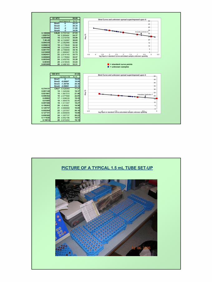
G1 NTC 50.00Log of input or Q Av. Ct

Stnd1 0 25.33Stnd2 -1 28.34Stnd3 -2 31.80Stnd4 -3 34.99

0.198088 CALB -0.703142 27.531.859791 14 0.269464 24.370.000489 15 -3.310705 35.99

7.5E-05 16 -4.124997 38.650.004335 17 -2.362966 32.920.006612 18 -2.179648 32.320.000598 19 -3.223083 35.700.001791 20 -2.746849 34.160.010095 21 -1.995907 31.720.002431 22 -2.614143 33.730.000665 23 -3.176984 35.570.003542 24 -2.450765 33.20

0.00303 25 -2.518545 33.430.003265 26 -2.486163 33.31 = standard curve points

= unknown samples

18S NTC 41.93Log input or Qty Av. Ct

Stnd1 0 16.03Stnd2 -0.69897 18.09Stnd3 -1.39794 20.36Stnd4 -2.09691 23.10

0.374137 CALF -0.426969 17.310.091145 14 -1.040266 19.370.021801 15 -1.661515 21.460.008362 16 -2.077668 22.85

0.09862 17 -1.006035 19.250.01085 18 -1.964578 22.47

0.097286 19 -1.011947 19.270.158263 20 -0.80062 18.560.129757 21 -0.886868 18.850.055264 22 -1.257557 20.100.127101 23 -0.895849 18.880.050382 24 -1.297727 20.230.111636 25 -0.952196 19.07

0.10612 26 -0.974204 19.15

Stnd Curve and unknown spread superimposed upon it

0

5

10

15

20

25

30

35

40

45

50

-4.5 -4 -3.5 -3 -2.5 -2 -1.5 -1 -0.5 0 0.5log Input or standard curve-calculated sample unknown quantity

Avg

. Ct

Interplate Calibrator B

Stnd Curve and unknown spread superimposed upon it

0

5

10

15

20

25

30

35

40

45

50

-2.5 -2 -1.5 -1 -0.5 0log Input or standard curve-calculated sample unknown quantity

Avg

. Ct

Interplate Calibrator F

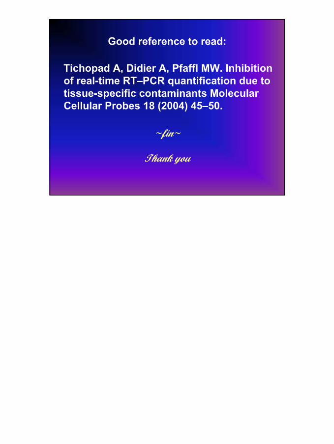
PICTURE OF A TYPICAL 1.5 mL TUBE SET-UP

8

PICTURE OF THE Eppendorf epMotion 5070 ROBOT IN ACTION

TYPICAL STORAGE OF qPCR PLATES AT 4oC BEFORE USE

9

Stratagene Mx3005P depiction of recent Test Plate resultsY-axis is shown in log units here – much easier to interpret results visually this way

Amplification plot

Standard Curve

93.7% Efficiency over a range of undiluted to 1:5,000,000-diluted RNA sample

10

Depiction of Amplification Curves on ABI 5700 sds software

h R SV q P C R a mp l i f i c a t i o n p r o f i l e a t d i f f e r e n t R N A s a mp l e c o n c e n t r a t i o n s

20

25

30

35

40

45

50

-6 -5 -4 -3 -2 -1 0[ l og] sa mpl e di l ut i on

Ct

Erroneous assessments

Correct log-linear quantitative region

qPCR dilution profile generated from purified viral (hRSV) inoculum: no inhibitory phenomena evident. …

Example showing how hRSV RNA virus gives faulty values when tissue total RNA sample is used too concentrated in the qPCR application:

Note: the inhibitory phenomena illustrated above does not manifest itself with Trizol-isolated viral RNA from purified viral inoculum; only with RNA Trizol-isolated from tissue.

The red-circled points are erroneous and suggest much lower viral presence than is actually the case. The blue line indicates those dilutions of the RNA sample which yield true quantitative results in the assay. The first blue-lined point which begins to behave in the desired fashion represents an in-well [RNA] of 0.1248 ng/uL. For three viral signals so far (bRSV, hRSV and PCV-2, a DNA virus), we have found 0.083 ng/uL to be a very good concentration at which to start using total tissue RNA (containing virus) for qPCR analyses.

The goal is to let this assay be as sensitive as possible. Diluting RNA samples out beyond their ability to generate qPCR signal at all is just as bad as not diluting RNA samples far enough.

11

Trizol RNA isolation is considerably cheaper than alternative methods. In cases where cost is not a factor, and tissues are being extracted for RNA, we would highly suggest using the Qiazol RNEasy Lipid Tissue Mini kit #74804 from Qiagen. For non-tissue samples (i.e. swabs and lavages) other RNA column-based isolation kits from Qiagen can be employed. A nice feature of these column-based RNA isolations is that inhibitory qPCR phenomena typically disappears from qPCR reactions when the RNA isolates are used after an in-well dilution of 1:50. Trizol-isolated RNA requires in-well dilutions of at least 1:200 before one can be confident that most tissue-related qPCR inhibitory phenomena is held at bay. (But again, remember that specific target template inhibition still needs tobe elimintaed by dilution as well; i.e. especially housekeepers).Marligen Rapid Total RNA purification system No. 11502-050 (Sandra Clark)The Trizol approach costs roughly $1.50 per each RNA sample isolated, while the Qiazol approach costs $5.40 per sample. So, realize that if you choose methods other than Trizol, your cost will increase by a factor of 3.5 or more.

hRSV in lamb lung

0

1

2

3

4

5

6

7

8

9

hRSV SBD-1 SP-D SP-A TTF-1

Control

hRSV

Example of results: target values in each case normalised to their respective housekeeper values. (Control animal qPCR

target levels versus hRSV-infected animal levels are compared).

12

Log2 Data Tranformations:hRSV SBD-1 SP-D SP-A TTF-1

Control lambs 0 0 0 0 0hRSV-infected lambs 10.09416 -1.46161 0.691547 0.167954 0.064018

sem hRSV SBD-1 SP-D SP-A TTF-1Control lambs 0.004608 -0.51937 0.055431 0.029679 0.00445

hRSV-infected lambs 2.664622 -0.2191 0.128381 0.023485 0.003287Alicia's 10-lamb study

hRSV in lamb lung; qPCR

-2

0

2

4

6

8

10

12

hRSV SBD-1 SP-D SP-A TTF-1

Rel

ativ

e ex

pres

sion

Control animal target expression levels become “zero” here (as a result of normalisingall housekeeper-normalised target values to control animal levels and then log base 2 transfroming those values). The result of this is then that infected animal target levels thus are shown as being above or below “zero”

The advantage of using these logarithmically transformed values is that they theoretically exhibit ‘normal distribution’, which is a precondition for the calculation of arithmetic mean values and further statistical analysis (e.g., t-test, f-test) …

Log base 2 versus Log base 10 transformed values

The “Bonn” Paperclick

-4

-2

0

2

4

6

8

10

0 1 2 3 4 5 6 7 8 9 10

Originalvalues

Log base 2

Log base 10

Log2 transformation study file

13

The PCR Equation: a 2The PCR Equation: a 2nn processprocess

Xn = X0(1 + E)n

Xn = PCR product after cycle nX0 = initial template numberE = amplification efficiencyn = cycle number

Xn

XX00cycle number

X0(2)n

Efficiency = 10[-1/slope] –1Ideal slope is always = -3.32192809488 or -1/log(2)

Slope? Slope of what? Answer: Any user-known sample dilution series tested for a qPCR target – also called “standard curves” or “dilution curves” or “calibration curves”. So, “slope” = the slope of the line describing log of sample dilution versus Ct. The user knows the dilutions she or he used.

Note here that the expression (1 + E) = “exponential amplification” – which tells you how close the qPCR reaction comes to doubling the template every cycle. If so, the reaction is 100% efficient and has attained the ideal “exponential amplification” value of 2.

And, Exponential Amplification = 10[-1/slope]

Log scale

Amplifications are assessed only during the phase of the reaction when the relationship between detected fluorescence and cycle number is log linear in nature: ideally for 3 cycles too…

And, interestingly …After applying some mathematical rules of logs to the above equation, we are able to further deduce that: 2∆Cti = fSo, with these two equations, assuming 100% reaction efficiency, we can calculate any expected qPCR Ct series; i.e. we can predict where each subsequent amplification should cross threshold.

Any deviations from these (ideal) predictions, thus, means that the qPCR amplification reaction at hand is other than 100% efficient …either lower or higher … (higher than 100%? – template or chemical inhibition, lower than 100%? – suboptimal reaction conditions including inappropriate primer, probe or template concentrations)

After a long while, I realized that: log10(f)/log10(2) = ∆Cti

• Where “f” = the sample dilution factor between any successive Ctsof any progressive dilution series,

• And, where “∆Cti” = the expected ideal number of cycles between any successive Cts of samples differing in concentration by dilution factor “f” (this assumes that the qPCR amplification reaction is 100% efficient; or “ideal”).

14

I find that qPCR Math boils down to a very simple equation from which all else can be derived:

2λ = f (in idealty) or λ log(2) = log(f ) (in idealty) or λ = log(f )/log(2)

where: λ = ∆CTi = the ideal expected frequency of appearance of Cts for any dilution series between or among samples

and f = the known dilution factor of the dilution between or among samples

Do not be afraid to dig through qPCR Math;

It is fairly straight-forward, interesting and enjoyable

Real-time qPCR Math Practice File

Click on this file to explore ideal and non-ideal qPCR mathematical situations

In the Swillins Manuscript:(Nucleic Acids Reasearch, 2004, Vol. 32, No. 6 e53):

The Equation becomes:(copy number)initial = [(∆Rn[probe]total)/(∆Rn,plateauEn)]VNo

for any single sampleWhere: here, "E" = Exponential Amplification

∆Rn = change in fluorescence during the linear log phase only

∆Rn,plateau = total change in fluorescence from baseline to plateauEn = the amplification factor in the exponential phase (EAMP)[probe]total = initially added concentration of fluorogenic probeV = sample volumeNo = Avogadro's number (6.0221367 x 1023)

Standard Curve still required here to estimate E reliably, however …

During the log linear phase only

From Baseline to final plateau

The Future of qPCR Math: The “Swillens Equation”may be able to interpret a single amplification curve like a fingerprint … The Swillens, et al. paper

15

Good reference to read:

Tichopad A, Didier A, Pfaffl MW. Inhibition of real-time RT–PCR quantification due to tissue-specific contaminants Molecular Cellular Probes 18 (2004) 45–50.

~fin~

Thank you