Galerkin method for feedback controlled Rayleigh–Bénard convection

This article has been downloaded from IOPscience. Please scroll down to see the full text article.

2008 Nonlinearity 21 2625

(http://iopscience.iop.org/0951-7715/21/11/008)

Download details:

IP Address: 129.67.186.247

The article was downloaded on 13/11/2011 at 22:29

Please note that terms and conditions apply.

View the table of contents for this issue, or go to the journal homepage for more

Home Search Collections Journals About Contact us My IOPscience

IOP PUBLISHING NONLINEARITY

Nonlinearity 21 (2008) 2625–2651 doi:10.1088/0951-7715/21/11/008

Galerkin method for feedback controlledRayleigh–Benard convection∗

A Munch1 and B Wagner2

1 Theoretical Mechanics Section, School of Mathematical Sciences, University of Nottingham,Nottingham NG7 2RD, UK2 Weierstrass Institute for Applied Analysis and Stochastics (WIAS), Mohrenstr. 39, 10117Berlin, Germany

E-mail: andreas.muench@nottingham.ac.uk and wagnerb@wias-berlin.de

Received 20 July 2007, in final form 8 August 2008Published 10 October 2008Online at stacks.iop.org/Non/21/2625

Recommended by A L Bertozzi

AbstractThe problem of feedback controlled Rayleigh–Benard convection is considered.For this problem with the simple flow structure in the vertical direction,a Galerkin method that uses only a few basis functions in this directionis presented. This approximation yields considerable simplification of theproblem, explicitly incorporates the non-classical boundary conditions at thehorizontal boundaries of the fluid layer resulting from feedback control andreduces the dimension of the original problem by one. This method is in spiritvery similar to lubrication theory, where the simple laminar flow in the verticaldirection is integrated out across the height of the fluid layer.

Using a minimal set of appropriate basis functions to capture the nonlinearbehaviour of the flow, we investigate the effects of feedback control onamplitude, wavelength and selection of patterns via weakly nonlinear analysisand numerical simulations of the resulting dimension-reduced problems in twoand three dimensions.

In the second part of this study we discuss the derivation of the appropriatebasis functions and prove convergence of the Galerkin scheme.

Mathematics Subject Classification: 74D10, 74F05, 74F10, 77N25

PACS numbers: 68.15.+e

(Some figures in this article are in colour only in the electronic version)

∗ This paper is published as part of a collection in honour of Todd Dupont’s 65th birthday.

0951-7715/08/112625+27$30.00 © 2008 IOP Publishing Ltd and London Mathematical Society Printed in the UK 2625

2626 A Munch and B Wagner

1. Introduction

Rayleigh–Benard convection occurs abundantly in nature, such as in oceans and theatmosphere, as well as in many technological processes, wherever heat transport or fluidmixing becomes relevant. Since the pioneering works by Lord Rayleigh [1] and Benard [2],numerous experimental and theoretical studies have been undertaken, in part because of therelative ease of producing accurate experimental data and on the other hand because of therich dynamical behaviour of the Rayleigh–Benard system, which plays a fundamental rolein the theory of pattern forming systems. Apart from some of the earliest theoretical studiesby Busse [3, 4] we refer here to [5] and more specifically [6] and [7] for a review and manyreferences therein.

In the most basic experimental setting Rayleigh–Benard convection arises when aquiescent fluid layer inside a closed container is heated from below. Above a certain verticaltemperature difference, quantified by the Rayleigh number (Ra), buoyancy forces destabilizethe fluid leading to the appearance of rolls and more complicated patterns as the temperaturedifference is increased. Experimental investigations of large-aspect-ratio Rayleigh–Benardsystems have led to the discovery of further instabilities, and for example the appearance ofspiral-defect chaos [8–11]. Apart from the aspect ratio and boundary effects from the sidewalls, these instabilities also depend on the value of the Prandtl number (Pr) and, for the caseof spiral-defect chaos, they even occur for parameter values where straight convection rolls arestable. Theoretical work is typically based on the one hand on the Boussinesq equation [12, 13]and on the other hand on model equations such as the Swift–Hohenberg model [14–16] andgeneralizations thereof. One disadvantage of the Swift–Hohenberg models is that there is norigorous derivation from the underlying Boussinesq equations and moreover for spiral-defectchaos these models may predict incorrect behaviour [17].

Apart from the scientific interest, for many technological applications it is important toinvestigate the feasibility of controlling and modifying the arising patterns such as describedabove. A typical example is Czochralski crystal growth [18], where during the growth processconvection in the melt may cause inhomogeneities of dopants. Here, suppression or delay ofonset of the instability is desirable. With respect to this objective it is desirable to explore thepotential of active feedback control and develop mathematical models and methods that allowfor an efficient treatment of the control problems at hand.

Experimentally, various strategies have been pursued in a series of works by Tang andBau [19–21] as well as by Howle [22–24], and more recently followed up by [25–28], wherethe onset of convection could be delayed by several factors of the critical Rayleigh number. Thebasic strategy, as pursued originally by Tang and Bau, is to cancel convection in the Rayleigh–Benard system by imposing a temperature distribution at the lower boundary in proportion toa measured temperature distribution in the middle of the fluid layer. Alternatively, control viaan imposed velocity distribution at the lower boundary was investigated. A different strategyis pursued by Howle. Here, the heat flux at the lower boundary is used as a feedback control,since prescribing the heat flux is experimentally easier. On the upper boundary an uniformtemperature is imposed and the velocity obeys the no-slip conditions on the upper and lowerboundaries. The control law specifies the spatial distribution of the heat flux on the lowerboundary while keeping the spatial mean heat flux constant. In this way the control of theheat flux acts so as to aid the natural dissipation in the system and as a consequence negativefeedback control delays the onset of convection.

In Howle’s experiments the wave pattern is obtained by shadowgraphic visualization ofthe state of the system. In order to use this as an input for the control law an expression for theshadowgraphic wave pattern, originally derived in [29], is used in the derivation of the condition

Galerkin method 2627

at the lower boundary. The active feedback control then sets the heat flux at the lower boundaryproportional to the shadowgraphic signal. In [30] comparison of the experimental results withpredictions of linear stability analysis of the negative feedback-controlled Boussinesq equationsshows good agreement. In [31] it was shown theoretically that positive feedback control ofthe Boussinesq equation may lead to an ill-posed problem, which is removed by an extensionof the model that includes more details of the control boundary, such as the thickness of theboundary. It is then shown that not only for negative but also for positive feedback control thedelay or advance of the onset of the instability remains bounded as the strength of the controlparameter is increased.

Via a mathematical model for this control mechanism, we will here also answer questionson the change in amplitude at the new critical conditions as the strength of the feedbackcontrol is varied and in higher dimensions investigate the impact on pattern selection. A goalof practical interest would certainly be to directly modify fluid patterns.

The contribution we intend to make in this direction is threefold:First, we make use of the property that while the convection patterns may have a

complicated structure in the horizontal large-scale directions, the flow field and the temperaturedistribution in the small-scale vertical direction are simple for the large-aspect ratios consideredin the experiments we discussed above.

In this case it is very convenient to use dimension-reduced models derived from theunderlying Boussinesq equation via a Galerkin approximation to efficiently explore thebifurcation structure of the control problem. The objective of the Galerkin approximationdiscussed here is to represent the flow variables by a linear combination of basis functions,using a small number (one or two) of low degree polynomials for the vertical direction, suchthat the boundary conditions are explicitly satisfied. Essentially it is a projection method thatprojects an approximate structure of the solution together with the original problem onto a spaceof basis functions, within which the approximated problem is solved. In this way the numberof spatial dimensions of the boundary value problem is reduced by one. This approximationcan be systematically derived from the underlying governing equations, here the Boussinesqequations, it is easily extendable to include higher order structures by allowing for more basisfunctions and its accuracy can be determined.

We note that it is similar in spirit to the lubrication approximation. There, one explicitlyuses the length-scale separation to reduce the Navier–Stokes equations and then integrates outthe dependence of the laminar flow in the vertical direction. Here, one has to incorporate asmall number of basis functions to account for the simple flow structure in one direction andupon integrating that out, to obtain a dimension-reduced problem.

We point out that the underlying idea of the Galerkin approximation is a generic conceptand similar approximations have also been developed by other groups. Most notably, the grouparound Pesch [12, 13] and Busse [4] who applied it to a number of problems related to Rayleigh–Benard convection such as for example convection in liquid crystals [32]. Furthermore,Manneville and coworkers used a similar Galerkin approximation in the context of Rayleigh–Benard convection in [33] and more recently also for other problems, such as for plane Couetteflow [34] and for flow down an inclined plane [35].

The derivation used in this study was originally inspired by [36]. They applied theirapproach to a variety of problems, including Rayleigh–Benard convection in 2D, formation ofshocks in suspensions or colloids. Their approach has been extended further to the Rayleigh–Benard problem that includes non-classical boundary conditions resulting from feedbackcontrol in [31]. Here, we go beyond linear analysis for the reduced models and furthermoreextend the approximation to three dimensions.

2628 A Munch and B Wagner

Second, the Galerkin method discussed in these studies is well suited to includecomplicated boundary conditions allowing us to use realistic and experimentally testedfeedback control mechanisms into our model and the perspective to compare with experimentalresults.

Third, we prove convergence of the approximation method.In the following section we formulate the feedback controlled Rayleigh–Benard problem

and derive dimension-reduced models for one and two basis functions. In section 3 we performa weakly nonlinear stability analysis. In section 4 we extend the derivation to three dimensionsand investigate numerically the patterns selected by applying feedback control. In section 5 weaddress the peculiarities of artificial singularities as they appear for positive feedback control.We observe that this already occurs for the central problem of the feedback controlled heatequation. We derive appropriate conditions for the basis function to resolve this problemand finally prove convergence of the resulting Galerkin scheme. We conclude with a shortdiscussion on spiral-defect chaos, derive the corresponding Galerkin approximation and showsome numerical results.

2. Formulation

The governing equations for the convection layer are the Boussinesq equation together withthe continuity and energy equations. In dimensionless form they are

Pr−1[∂tu + (u · ∇)u] = −∇p + R T + (0, 0, 1)t + ∇2u, (2.1)

∇ · u = 0, (2.2)

∂tT + u · ∇T = ∇2T + w, (2.3)

where the scalings

(x, y, z) =(

x∗

d,y∗

d,z∗

d

), t = κ

d2t∗, (u, v, w) = d

κ(u∗, v∗, w∗),

T + = k

qdT ∗, p = d2

ρκ2p∗.

(2.4)

have been used. We denote by d , κ , ρ and q the height of the fluid layer, thermal diffusivity,fluid density and spatially averaged heat flux, respectively. We further write

u = (u, v, w), T + = Tc + T = θu −(

z − 1

2

)+ T (2.5)

with the conductive state Tc and the temperature θu on the upper boundary z = 1/2.

R = gαqd4

κνkthand Pr = ν

κ(2.6)

denote the Rayleigh and the Prandtl number, with kth, α, g and ν the thermal conductivity,thermal expansion coefficient, gravity and viscosity, respectively. Except for the treatment ofthe spiral-defect chaos we assume the Prandtl number to be large and therefore neglect theleft-hand side of (2.1). This is in accordance with the experimental situation of [22].

We assume solutions are periodic in x and y and satisfy no-slip and no-penetrationconditions at the upper and lower boundaries

u = v = w = 0 at z = ± 12 . (2.7)

In experiments by [24] the temperature is kept fixed at the upper boundary. Hence, we have

T = 0 at z = + 12 . (2.8)

Galerkin method 2629

The feedback control boundary condition at the lower boundary is derived as follows.The spatial distribution of the heat flux q at the lower boundary is set proportional to theshadowgraphic signal. In addition the heat flux is also set proportional to the time derivativeof the shadowgraphic signal in [23], but we will neglect this contribution here. The heat fluxq = −kth∂zT is then given by

q = q

(1 + c

δI (x)

I0

), (2.9)

where c is a proportionality factor of the shadowgraphic signal δI (x)/I0, I0 being the uniformbrightness at reference state. An expression for the shadowgraphic signal in terms of thetemperature was derived in [29] and is given by

δI (x)

I0= −2H

dη

dT2

∫ d/2

−d/2T dz (2.10)

as long as the ratio of the height of the fluid layer d over the distance of the fluid layer tothe image plane H is large. Here, η denotes the refractive index, which usually decreases asthe temperature increases, i.e. dη/dT is negative. Hence the dimensionless expression for T

in (2.5) is

∂zT = −ω 2

∫ 1/2

−1/2T dz at z = −1

2, (2.11)

where 2 = ∂2x + ∂2

y and the dimensionless proportionality factor

ω = 2cH

d

(− dη

dT

)(2.12)

is the control parameter. Hence for positive c (i.e. negative feedback control), ω > 0.Moreover, the integral of the shadowgraphic signal over x and y is zero, so that the globalRayleigh number is not altered by the control.

In [31] it was also found that the problem may become ill posed for ω < −1, i.e. for acritical positive proportionality factor. This is readily understood for the much simpler linearproblem for the heat equation ∂tT = T with control boundary condition (2.11) at z = −1/2and no-flux boundary condition ∂zT = 0 on the upper boundary z = 1/2. Integrating the heatequation from z = −1/2 to z = 1/2 and taking the Fourier transform of the result in the lateraldirections gives

∂t T (k, t) = −(ω + 1)k2T (k, t), where T (k, t) =∫ 1/2

−1/2

∫e−ikzT (x, z, t) dx dz,

given here in two dimensions for simplicity. It is now easily seen that the one-dimensionalspectrum decays like a diffusion process with −(ω + 1) as the diffusion coefficient. Clearly,ω < −1 yields a diffusion process which is backward in time and renders the problem ill-posedin the sense that perturbations at high wave number k are amplified at a rate proportional tok2. This and the extension of this argument to positive feedback-controlled Rayleigh–Benardconvection is given in detail in [31], as well as the treatment of the extended model that takesinto account boundary properties such as boundary thickness or heater size.

2.1. Galerkin method

We first briefly present the derivation of the dimension-reduced problem in 2D for simplicity,see also [31]. We begin by representing the flow variables by a linear combination of basisfunctions, using only a small number of low degree polynomials for the z-direction. By testing

2630 A Munch and B Wagner

z = 1/2

z =-1/2

u > 0 u = 0 u < 0 T

z = 1/2z = - 1/2

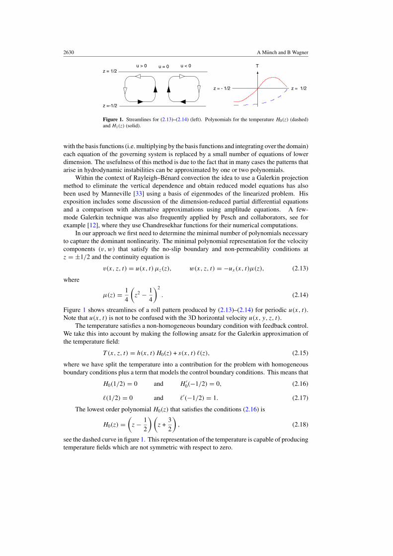
Figure 1. Streamlines for (2.13)–(2.14) (left). Polynomials for the temperature H0(z) (dashed)and H1(z) (solid).

with the basis functions (i.e. multiplying by the basis functions and integrating over the domain)each equation of the governing system is replaced by a small number of equations of lowerdimension. The usefulness of this method is due to the fact that in many cases the patterns thatarise in hydrodynamic instabilities can be approximated by one or two polynomials.

Within the context of Rayleigh–Benard convection the idea to use a Galerkin projectionmethod to eliminate the vertical dependence and obtain reduced model equations has alsobeen used by Manneville [33] using a basis of eigenmodes of the linearized problem. Hisexposition includes some discussion of the dimension-reduced partial differential equationsand a comparison with alternative approximations using amplitude equations. A few-mode Galerkin technique was also frequently applied by Pesch and collaborators, see forexample [12], where they use Chandresekhar functions for their numerical computations.

In our approach we first need to determine the minimal number of polynomials necessaryto capture the dominant nonlinearity. The minimal polynomial representation for the velocitycomponents (v, w) that satisfy the no-slip boundary and non-permeability conditions atz = ±1/2 and the continuity equation is

v(x, z, t) = u(x, t) µz(z), w(x, z, t) = −ux(x, t)µ(z), (2.13)

where

µ(z) = 1

4

(z2 − 1

4

)2

. (2.14)

Figure 1 shows streamlines of a roll pattern produced by (2.13)–(2.14) for periodic u(x, t).Note that u(x, t) is not to be confused with the 3D horizontal velocity u(x, y, z, t).

The temperature satisfies a non-homogeneous boundary condition with feedback control.We take this into account by making the following ansatz for the Galerkin approximation ofthe temperature field:

T (x, z, t) = h(x, t) H0(z) + s(x, t) �(z), (2.15)

where we have split the temperature into a contribution for the problem with homogeneousboundary conditions plus a term that models the control boundary conditions. This means that

H0(1/2) = 0 and H ′0(−1/2) = 0, (2.16)

�(1/2) = 0 and �′(−1/2) = 1. (2.17)

The lowest order polynomial H0(z) that satisfies the conditions (2.16) is

H0(z) =(

z − 1

2

) (z +

3

2

), (2.18)

see the dashed curve in figure 1. This representation of the temperature is capable of producingtemperature fields which are not symmetric with respect to zero.

Galerkin method 2631

This is not so, if for example we had chosen Neumann boundary conditions on both sides,see [36]. In this case we would have needed a third order polynomial as well in order to breakthe symmetry of the temperature profile.

In section 5 we show that the polynomial �(z) not only needs to satisfy conditions (2.17)but also in order to prevent artificial singularities that arise through this approximation, forpositive feedback control, we need to require

ρ1 =∫ 1/2

−1/2�(z) dz = 〈�, H0〉

∫ 1/2

−1/2H0(z) dz (2.19)

with

〈�, H0〉 =∫ 1/2

−1/2�(z)H0(z) dz. (2.20)

We give a derivation of this in section 5. In order to simplify calculations we choose �(z) tobe orthogonal to H0(z), i.e. the scalar product 〈�, H0〉 = 0, and therefore also ρ1 = 0. Thisleads us to the polynomial

�(z) =(

z − 1

2

) (z2 +

1

8z − 1

16

). (2.21)

We obtain the Galerkin approximation by testing the full problem with the functions

θ0 = δ(x) µz(z), θ1 = −δ′(x) µz(z), φ0 = δ(x)H0(z), (2.22)

to obtain

∂4xu − 24 ∂2

xu + 504 u = −R ∂x

(60 h − 3

2s

), (2.23)

∂th − ∂2xh +

5

2h +

9

448

(u∂xh +

1

2h∂xu

)

= 15

8s +

5

448∂xu +

u∂xs − 3/2 s ∂xu

448 · 24. (2.24)

Finally, introducing (2.15) and (2.21) into the control boundary condition (2.11) yields

s = ω 23∂2

xh. (2.25)

The system of partial differential equations are not only much easier to treat numericallybecause of the reduced dimension, but, as we will see in the following section, its analyticaltreatment is much simpler.

3. Weakly nonlinear stability

We first recall from [31] that for this Galerkin approximation, linearization about the conductivestate h(x, t) = 0, u(x, t) = 0, reduces the linear stability problem to solving

∂t h = σ(k, ω)h (3.1)

with growth rate

σ(k, ω) = −(

k2 +5

2

)+

75

112MR + ωk2

(5

448MR − 5

4

). (3.2)

h(k, t) denotes the Fourier transform of h(x, t) and

M = k2

k4 + 24 k2 + 504, (3.3)

2632 A Munch and B Wagner

which yields the critical Rayleigh number as a function of the feedback control parameter,

Rc(ω) = 28

15

(4 + 5ω)(k4c + 24k2

c + 504)2

(2ω − 5) k4c + 84ωk2

c + 2520, (3.4)

where kc(ω) is the solution of the polynomial

(4 + 5ω)(ωk8 + 120k6) + (6360 + 4944ω − 2520ω2)k4 (3.5)

−10080ωk2 − 302400 = 0. (3.6)

The approximation yields rather good results, even though only one basis function has beenused. For example when ω = 0 (uncontrolled Rayleigh–Benard convection with rigidboundaries and Dirichlet/Neumann conditions for the temperature) we have Rc = 1446 andkc = 2.39 for the reduced model (with one basis function for the temperature) compared withRc = 1296 and kc = 2.55 for the full Boussinesq equations (2.1)–(2.11), which is a differenceof about 12% and 6%, respectively. The accuracy can be easily improved by using more basisfunctions. For example, if we use a two-function model, which is the reduced model obtainby the Galerkin method using two basis functions for the temperature (instead of one), thenwe obtain Rc = 1350 and kc = 2.52. This is a difference of just 4% and 1%, respectively.The reduced model for two basis functions and the linear stability analysis for it is included inappendix A.2.

The nonlinear behaviour near Rc is described by the Landau equations for theamplitude. Their derivation from the original governing equations is often problematic ifthe boundary conditions are other than Neumann conditions. The Galerkin approximationremoves boundaries in the z-direction. We show how the Landau equation for feedbackcontrolled Rayleigh–Benard convection can be derived on the basis of multiple-scaleasymptotics.

Suppose the system experiences a small initial perturbation

w(x, 0) = δ(u(x), h(x)), w = (u, h), (3.7)

where δ � 1. When we rescale the problem by δ as

u = δu∗, h = δh∗, (3.8)

drop the ∗ and denote

Lu(w) := ∂4xu − 24 ∂2

xu + 504 u + R ∂x

(60 h − 3

2s

), (3.9)

Lh(w) := ∂th − ∂2xh +

5

2h − 15

8s − 5

448∂xu, (3.10)

then, in the scaled problem, the nonlinear terms appear as a small correction:

Lu(w) = 0, (3.11)

Lh(w) = δ

448

[−9

(u∂xh +

1

2h∂xu

)+

ω

24

(2

3u∂xxxh − ∂xxh∂xu

)]. (3.12)

In the x-direction we assume periodic boundary conditions. For this perturbation problem wemake the ansatz

w(x, t; δ) := w0(x, t, τ ) + δw1(x, t, τ ) + δ2w2(x, t, τ ) + O(δ3), (3.13)

R = Rc + δ2α, τ = δ2t. (3.14)

Galerkin method 2633

To leading order we basically get the linear stability problem

Lu(w0) = 0, Lh(w0) = 0, (3.15)

with initial conditions: w0(x, 0) = (u(x), h(x)). (3.16)

To O(δ) we get

Lu(w1) = 0, (3.17)

Lh(w1) = 1

448

(−9

[u0∂xh0 +

1

2h0∂xu0

]+

ω

24

[2

3u0∂xxxh0 − ∂xxh0∂xu0

]). (3.18)

To O(δ2) we find

Lu(w2) = − α (60 ∂xh0 − ω∂xxxh0) , (3.19)

Lh(w2) = −∂τh0 − 9

448

(u1∂xh0 + u0∂xh1 +

1

2(h0∂xu1 + h1∂xu0)

)

+ω

448 · 24

(2

3u0∂xxxh1 +

2

3u1∂xxxh0 − ∂xxh0∂xu1 − ∂xxh1∂xu0

). (3.20)

Since we have periodic boundary conditions the solution can be written in the form

h0(x, t, τ ) =∞∑

n=1

An(t, τ ) sin(nkcx) + Bn(t, τ ) cos(nkcx), (3.21)

u0(x, t, τ ) =∞∑

n=1

En(t, τ ) sin(nkcx) + Fn(t, τ ) cos(nkcx), (3.22)

with

An(t, τ ) = K(τ)eσnt , Bn(t, τ ) = L(τ)eσnt

En(t, τ ) = VnAn(t, τ ), Fn(t, τ ) = −VnBn(t, τ ),

Vn = RcMn

nkc

(60 + ω(kcn)2

), Mn = (nkc)

2

(nkc)4 + 24(nkc)2 + 504,

σn = −(

(nkc)2 +

5

2

)+

75

112MnRc + ω(kcn)2

(5

448MnRc − 5

4

).

The leading order solution corresponds to the solution to the linear stability problem atcriticality. This means that there σ1 = 0, while for all other σin we have Re(σin) < 0.Hence, the dominant terms in the expansions are

h0 = K(τ) sin(kcx) + L(τ) cos(kcx), u0 = V1 [L(τ) sin(kcx) − K(τ) cos(kcx)] (3.23)

while all other terms decay.The unknown functions K(τ) and L(τ) have to be determined by solving the higher order

problems. To O(δ) we obtain the solution

h1 = ρ1(K2 + L2) + ρ2

[(L2 − K2) cos(2kcx) − 2KL sin(2kcx)

], (3.24)

u1 = q1[(L2 − K2) sin(2kcx) − 2KL cos(2kcx)

], (3.25)

2634 A Munch and B Wagner

where

ρ1 = V1kc

448

(9

10+ ω

k2c

72

), ρ2 = V1kc

448σ2

(27

4+ ω

k2c

144

),

q1 = 1

448

V1V2kc

σ2

(27

4− ω

k2c

144

).

Note that the right-hand side of (3.19)–(3.20) contains linear combinations of sin(kcx), cos(kcx)

etc. Hence, we make the following ansatz for the solution to u2 and h2:

u2 = µ1(τ ) sin(kcx) + ν1(τ ) cos(kcx), h2 = µ2(τ ) sin(kcx) + ν2(τ ) cos(kcx). (3.26)

If we now sort both sides of the O(δ2) equation with respect to sin(kcx) and cos(kcx) we obtainfour equations for the unknowns µ1, ν1, µ2, ν2. In vector notation this reads

1 0 0 −RcM1ζ

0 1 RcM1ζ 00 0 σ1 00 0 0 σ1

µ1

ν1

µ2

ν2

=

αLζ

−αKζ

Equation for K

Equation for L

, (3.27)

where

ζ = M1(60 + ωk2

c

)kc(ω)

and σ1 = σ1 (kc(ω), Rc(ω)) .

Note that σ1(kc(ω), Rc(ω)) = 0. Therefore, the solvability condition requires that the equationfor K and the equation for L on the right-hand side are zero:

dK

dτ− a(α, ω) K − b(ω) K (K2 + L2) = 0, (3.28)

dL

dτ− a(α, ω) L − b(ω) L (K2 + L2) = 0, (3.29)

where

a(α, ω) = 5

448αM1(60 + ωk2

c ),

b(ω) = kc

448

[9V1

(ρ1 − 1

2ρ2

)− ωk2

c

24

(4

3q1 +

14

3ρ2V1

)].

These are often also called the Landau equations. From linear theory we note that

sgn(a) = sgn(α) = sgn(R − Rc)

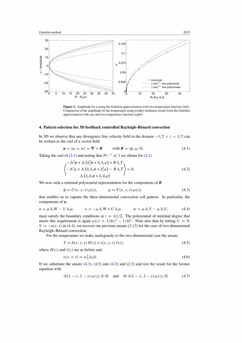
and that b(ω) > 0, so that we always have a supercritical bifurcation for any ω. We findthat feedback control decreases amplitudes if feedback control is positive, while they areincreased for negative feedback control. This is illustrated in figure 2 for the u-amplitudesfor ω = −0.9, −0.4, 0.4, 0.9. On the right of figure 2 we compare the results of the weaklynonlinear analysis to the numerical solution of the Galerkin model for ω = −0.4 for theh-amplitude.

Galerkin method 2635

0 5 10 15 20 25 30 35 40 45R – Rc(ω)

–30

–20

–10

0

10

20

30u

– A

mpl

itude

0 10 20 30 40R–Rc(–0.4)

0

0.025

0.05

0.075

0.1

0.125

h

numerical(–a/b)

1/2 one polynomial

(–a/b)1/2

two polynomials

Figure 2. Amplitude for u using the Galerkin approximation with two temperature function (left).Comparison of the amplitude for the temperature using weakly nonlinear results from the Galerkinapproximation with one and two temperature function (right)

4. Pattern selection for 3D feedback controlled Rayleigh–Benard convection

In 3D we observe that any divergence free velocity field in the domain −1/2 < z < 1/2 canbe written as the curl of a vector field

u = 〈u, v, w〉 = ∇ × B with B = 〈φ, ϕ, 0〉. (4.1)

Taking the curl of (2.1) and noting that Pr−1 � 1 we obtain for (2.1)

⟨−2φ + (∂2xφ + ∂y∂xϕ

)+ R ∂yT

−2ϕ + (∂x∂yφ + ∂2

yϕ) − R ∂xT

(∂x∂zφ + ∂y∂zϕ

)⟩

= 0. (4.2)

We now seek a minimal polynomial representation for the components of B

φ = U(x, y, t) µ(z), ϕ = V (x, y, t) µ(z), (4.3)

that enables us to capture the three-dimensional convection cell pattern. In particular, thecomponents of u,

u = µ ∂yW − V ∂zµ, v = −µ ∂xW + U ∂zµ, w = µ ∂xV − µ ∂yU, (4.4)

must satisfy the boundary conditions at z = ±1/2. The polynomial of minimal degree thatmeets this requirement is again µ(z) = 1/4(z2 − 1/4)2. Note also that by letting U = 0,V = −u(x, t) in (4.4), we recover our previous ansatz (2.13) for the case of two-dimensionalRayleigh–Benard convection.

For the temperature we make analogously to the two-dimensional case the ansatz

T = h(x, y, t) H(z) + s(x, y, t) �(z), (4.5)

where H(z) and �(z) are as before and

s(x, y, t) = ω 232h. (4.6)

If we substitute the ansatz (4.3), (4.5) into (4.2) and (2.3) and test the result for the formerequation with

〈δ(x − x, y − y) µ(z), 0, 0〉 and 〈0, δ(x − x, y − y) µ(z), 0〉 (4.7)

2636 A Munch and B Wagner

and the result for (2.3) with

δ(x − x, y − y) H(z) (4.8)

respectively, we obtain the problem

∂4yU − 24 ∂2

yU + 504 U + ∂2x

(∂2yU − 12 U

)= −R ∂y

(60 h − 3

2s

)+ ∂x∂y (2V − 12 V ) , (4.9)

∂4xV − 24 ∂2

xV + 504 V + ∂2y

(∂2xV − 12 V

)= R ∂x

(60 h − 3

2s

)+ ∂x∂y (2U − 12 U) , (4.10)

∂th − 2h +5

2h +

9

448

[(U ∂yh − V ∂xh

)+

1

2

(∂yU − ∂xV

)h

]

= 15

8s +

5

448

(∂yU − ∂xV

)(4.11)

+1

448 · 24

[(U∂ys − V ∂xs

) − 3

2

(∂yU − ∂xV

)s

]. (4.12)

We solve this system numerically using a finite difference method together with an implicitEuler scheme for the time discretization and a Newton scheme combined with an iterativesolver BICSTAB [37]) for the linear subproblems. We solve the problem with homogeneousDirichlet boundary conditions on an (Lx, Ly) square. For the initial condition we use

h(x, y, 0) = xy

(x

Lx

− 1

) (y

Ly

− 1

)10−n, (4.13)

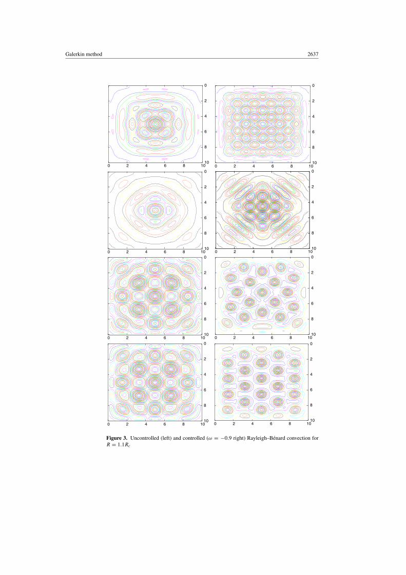
where we let n = 4. The other variables we set to zero. For all runs we let the Rayleighnumber R = 1.1 ∗ Rc. For the uncontrolled problem we expect a pattern of square convectioncells, for Dirichlet and Neumann boundary conditions on z = 1/2 and z = −1/2, respectively.Figure 3 shows the streamlines of the vertical velocity. We see in the first column, that aftergoing through a transient phase of a lozenges pattern, square cells start to appear and fill thewhole horizontal domain, as expected.

We now ask whether feedback control not only suppresses (or enhances) the instability aswell as changes its wavelength, but whether it can also have an effect on the three-dimensionalpattern. Starting with the same initial condition, we observe in the right column of figure 3that for feedback control of ω = −0.9 also here a lozenges pattern appears at first, followed bya pattern of square cells, all having smaller wavelength. Interestingly, at some point, when theamplitude has become large enough, the control effects a change in the up–down symmetryand a new hexagonal pattern eventually establishes itself and remains in this new state. Thisis a remarkable and new effect and it hints at a nontrivial response of the system with respectto feedback control, that needs to be explored further.

One focus of this study is to rigorously establish the convergence of our Galerkin methodbefore we go into more detail of the bifurcation structure of the reduced model.

5. Convergence

As we have already noted earlier in the text, feedback control may introduce new aspects thatneed to be dealt with for the expansion of the basis functions. In particular, positive feedback

Galerkin method 2637

0

2

4

6

8

10 0 2 4 6 8 10

0

2

4

6

8

10 0 2 4 6 8 10

0

2

4

6

8

10 0 2 4 6 8 10

0

2

4

6

8

10 0 2 4 6 8 10

0

2

4

6

8

10 0 2 4 6 8 10

0

2

4

6

8

10 0 2 4 6 8 10

0

2

4

6

8

10 0 2 4 6 8 10

0

2

4

6

8

10 0 2 4 6 8 10

Figure 3. Uncontrolled (left) and controlled (ω = −0.9 right) Rayleigh–Benard convection forR = 1.1Rc

2638 A Munch and B Wagner

control introduces artificial singularities into the dimension-reduced problem. We note that isalready a property of the core problem of the feedback controlled heat equation. We addressthis problem in the following section and show that additional conditions have to be satisfied,which in turn result in a modification of the basis functions. For the resulting Galerkin schemewe then prove convergence.

5.1. Artificial singularities

We now discuss the problem of artificial singularities for the two-dimensional heat equationwith boundary conditions resulting from feedback control. This problem can be furthersimplified if we Fourier transform it with respect to x,

Tt = Tzz − k2 T , (5.1)

Tz(1/2, t) = 0, (5.2)

Tz(−1/2, t) = ω k2∫ 1/2

−1/2T dz, (5.3)

T (z, 0) = g(z). (5.4)

Let us assume that this problem has a solution. We can always find a function �(z) such that�′(1/2) = 0 and �′(−1/2) = 0. Next we can define the following functions

s(t) = ω k2∫ 1/2

−1/2T dz, (5.5)

v(z, t) = T (z, t) − �(z) s(t), (5.6)

so that v(z, t) satisfies the equation

vt + � st = vzz − k2 v + (�′′ − k2 �) s (5.7)

with homogeneous boundary conditions

vz(1/2, t) = 0, (5.8)

vz(−1/2, t) = 0. (5.9)

For the initial conditions for v we note that from (5.5)–(5.6)

T (z, 0) = g(z) = v(z, 0) + �(z) s(0), (5.10)

= v(z, 0) + �(z)ωk2

1 − ρωk2

∫ 1/2

−1/2v(z, 0) dz, (5.11)

where

ρ =∫ 1/2

−1/2�(z) dz.

Integration of (5.11) yields∫ 1/2

−1/2v(z, 0) dz = (1 − ρω k2)

∫ 1/2

−1/2g(z) dz

and hence

v(z, 0) = g(z) − ω k2�(z)

∫ 1/2

−1/2g(z) dz. (5.12)

Galerkin method 2639

Conversely, it is clear that for given v that satisfies (5.7)–(5.9), with s and � having the aboveproperties, we can define T that satisfies (5.1)–(5.4).

Clearly, if we integrate (5.7) and denote

V (t) =∫ 1/2

−1/2v(z, t) dz and γ =

∫ 1/2

−1/2g(z) dz (5.13)

we see immediately that the resulting initial value problem

Vt = −(ω + 1) k2 V with V (0) = γ (1 − ρωk2) (5.14)

will be ill-posed for ω < −1, so this is a property of the full problem and has been explainedearlier in [31].

For our Galerkin approximation we proceed in a similar fashion. We approximatev(z, t) by

vN(z, t) =N∑i

Hi(z) hi(t), (5.15)

where the Hi form a sequence of orthonormal polynomials with respect to the standard innerproduct,

〈Hi, Hj 〉 =∫ 1/2

−1/2Hi(z)Hj (z) dz = δij , (5.16)

which satisfy

H′i (1/2) = 0, H

′i (−1/2) = 0, (5.17)

and set

TN(z, t) = vN(z, t) + �N(z) s(t), (5.18)

where �N(z) is a polynomial with

�′N(1/2) = 0, �

′N(−1/2) = 1. (5.19)

Substitution of (5.18) into (5.1)–(5.3) and taking the inner product with Hj yields for each j

the equation

hj t+ 〈�N, Hj 〉 st =

N∑i

〈H ′′i , Hj 〉hi − k2 hj + 〈�′′

N− k2�N, Hj 〉s, (5.20)

s(t) = ωk2

1 − ρNωk2

∫ 1/2

−1/2vN dz with ρN =

∫ 1/2

−1/2�N dz. (5.21)

The problem for vN(z, t) is now obtained by summation of the product of Hj and (5.20). Ifwe integrate the resulting equation by using (5.21) as well as the properties of Hi and �N anddenote

VN(t) =∫ 1/2

−1/2

N∑j

Hj hj dz =∫ 1/2

−1/2vN dz, (5.22)

and the projection

P(Q) =N∑i

〈Q, Hj 〉Hj, (5.23)

2640 A Munch and B Wagner

for some polynomial Q, we obtain the following equation[1 + ω k2

(∫ 1/2

−1/2P(�N) − ρN dz

)]VN t = −k2

[1 + ω + ω k2

(∫ 1/2

−1/2P(�N) − ρN dz

)]VN

+ ω k2

[∫ 1/2

−1/2P(�

′′N) − �

′′N

dz

]VN +

(1 − ρNωk2

) ∫ 1/2

−1/2

N∑i

[P(H

′′i ) − H

′′i

]hi dz.

In this form, we observe that, for ω < 0, the approximate problem will produce artificialsingularities, which are not present in the exact problem, if

1 + ω k2

(∫ 1/2

−1/2P(�N) − ρN dz

)= 0.

However, the sequence of orthonormal polynomials Hi that produce the approximation vN , allhave property (5.17). Hence the constant polynomial H0(z) = 1 is always a member. But thismeans that ∫ 1/2

−1/2P(Q) dz = 〈Q, H0〉 =

∫ 1/2

−1/2Q dz. (5.24)

Therefore, (5.24) reduces to

VN t = −(1 + ω) k2 VN with VN(0) = γ (1 − ρNωk2). (5.25)

Property (5.24), however, is not necessarily satisfied for general boundary condition. If wechange, for example, the top (z = 1/2) boundary condition to be of the Dirichlet type, thenHi(1/2) = 0 and (5.24) cannot be derived anymore. Therefore, if we want to approximateproblem (5.1)–(5.4) with T (1/2, t) = 0, by (5.15)–(5.19) with Hi(1/2) = 0 and �N(1/2) = 0,we again find the same coefficient of VN t . In this case, however, we have to explicitly require∫ 1/2

−1/2�N dz =

∫ 1/2

−1/2P(�N) dz (5.26)

in order to avoid artificial singularities for negative ω. This in turn gives an additional constrainton �N , leading to the new basis function (2.21).

5.2. Convergence proof

For the problem

Tt = Txx + Tzz on �, (5.27)

Tz(x, 1/2, t) = 0, (5.28)

Tz(x, −1/2, t) = −ω

∫ 1/2

−1/2Txx dz, (5.29)

T (x, z, 0) = g(x, z), (5.30)

where � denotes the domain ]0, L[ × ] − 1/2, 1/2[, and where T satisfies periodic boundaryconditions in x, and t ∈ [0, tf ], we analyse the convergence properties of a Galerkin schemedesigned to approximate the solution of (5.27)–(5.30). For later use, we set I :=] − 1/2, 1/2[.For this purpose, we first make some assumptions regarding the solution of the continuousproblem. We will assume that for ω > −1 the problem has, for sufficiently smooth datag, a unique solution with T ∈ L2(H 2(�)), and that this solution has additional regularityproperties, T and Tt ∈ L2(H 7/2(�)).

Galerkin method 2641

In the next paragraph, we reformulate the continuous problem by splitting T into twovariables, θ , that satisfies homogeneous boundary conditions at z = ±1/2, and a second terms(x, t)l(z) which accounts for the control boundary conditions (5.29). We also pass to theFourier-transform with respect to x. In section 5.2.2, we will set up the weak formulation andthe Galerkin scheme. In section 5.2.3 we derive estimates for the difference of the solution T

and the discrete solution T N in terms of the norm of the continuous solution for θ . The boundfor the difference of T and T N provided by this estimate tends to zero as N tends to ∞, whereN is the dimension of the sub-space used for the discretization.

5.2.1. Reformulation. Now fix a polynomial l(z) so that

l′(1/2) = 0, l′(−1/2) = 1 and∫ 1/2

−1/2l dz = 0,

and let

s(x, t) = Tz(x, −1/2, t), (5.31)

θ(x, z, t) = T (x, z, t) − s(x, t)l(z) (5.32)

for t � 0. Then, s and θ , θt are in L2(H 2(]0, L[)) and L2(H 2(�)), respectively, and satisfy

θt + st l = θxx + θzz + sxxl + sl′′, (5.33)

s = −ω

∫ 1/2

−1/2θxx dz, (5.34)

θz(x, ±1/2, t) = 0, (5.35)

s(x, 0) = gz(x, −1/2), (5.36)

θ(x, z, 0) = g(x, z) − s(x, 0)l(z). (5.37)

Conversely, any solution s and θ of (5.33)–(5.37) of this regularity class generates via

T (x, z, t) = θ(x, z, t) + s(x, t)l(z) (5.38)

a solution of (5.27)–(5.30) within the class L2(H 2(�)) (or better). Since we assumed that thesolution T of (5.27)–(5.30) is unique, the solution s and θ of (5.33)–(5.37) must be unique too.For, assume we have two solutions, s1, θ1 and s2, θ2, then from uniqueness of T , it follows

θ1(x, z, t) + s1(x, t)l(z) = θ2(x, z, t) + s2(x, t)l(z). (5.39)

Evaluating this at z = −1/2 yields s1 = s2 and plugging this into (5.39) yields θ1 = θ2.In the following, we will assume that the solution (5.33)–(5.37) has additional regularity

properties,

s(t) ∈ H 2(]0, L[) and θ(t) ∈ H 2(�) both for all t ∈ [0, tf ]. (5.40)

We now Fourier transform (5.33)–(5.37), via

s(x, t) =∞∑

j=0

s(j, t)eikj x, θ(x, z, t) =∞∑

j=0

θ (j, z, t)eikj x with kj = 2π

Lj.

2642 A Munch and B Wagner

In the following, we will typically suppress the dependence on j , e.g. by writing k instead ofkj . The transformed equations then read

θt + st l = −k2θ + θzz − k2sl + sl′′, on I, and for t > 0 (5.41)

s = ωk2∫ 1/2

−1/2θ dz, on I, and for t > 0, (5.42)

θz(j, ±1/2) = 0, (5.43)

s(j, 0) = gz(j, −1/2), (5.44)

θ (j, z, 0) = g(j, z) − s(j, 0)l(z). (5.45)

These equations have to be solved for all j = 0, 1, . . .. From our above considerations, weconclude that (5.41)–(5.45) can be assumed to have, for each j , a unique solution s, θ withinthe class of functions that satisfy

θ (t) ∈ H 2(I ), for all t ∈ [0, tf ] (5.46)

and ∫ tf

0|s|2 dt < ∞ and θ ∈ L2H 2(I )).

5.2.2. Weak formulation and discretization. Let

Mc := {ψ ∈ H 2(I ); ψz(±1/2) = 0}.Then, for the above solution we have θ (t) ∈ Mc and θ , s satisfy (where (·, ·) denotes the innerproduct of L2(I )),

(θt , ψ) + st (l, ψ) = −(θz, ψz) − s(l′, ψz) − sψ(−1/2) − k2(θ , ψ) − k2s(l, ψ),

for all ψ ∈ Mc. (5.47)

The remaining conditions, (5.42)–(5.45), carry over from before.For the discrete subspaces of Mc, we take

MN := span{H0, H1, . . . , HN },where Hi are polynomials in z, ordered by their degree, that satisfy

H′i (±1/2) = 0, (Hi , Hj ) = δij . (5.48)

Note that, in particular, H0 ≡ 1. We then formulate the following problem (discretized withrespect to z):

Find sN , θN , with θN (t) ∈ MN , so that

(θNt , ψ) + sN

t (l, ψ) = −(θNz , ψz) − sN (l′, ψz) − sNψ(−1/2) − k2(θN , ψ) − k2sN (l, ψ),

for all ψ ∈ MN, (5.49)

sN = ωk2∫ 1/2

−1/2θN dz (5.50)

sN (j, 0) = s(j, 0) (5.51)

θN (j, z, 0) =N∑

i=0

(θ(j, ·, 0), Hi ) Hi(z). (5.52)

Galerkin method 2643

By setting ψ = 1 in (5.47) and in (5.49), respectively, we find that s and sN satisfy the sameequation,

st = −(1 + ω)k2s and sNt = −(1 + ω)k2sN ,

so that in view of (5.51), we get s(j, t) = sN (j, t) for all t ∈ [0, tf ]. Therefore, when wesubtract (5.47) and (5.49), all s and sN terms cancel

(θt − θNt , ψ) = −(θz − θN

z , ψz) − k2(θ − θN , ψ). (5.53)

5.2.3. Error analysis. Let πN : Mc → MN denote a projection onto MN , and let

ζ := θ − πN(θ), ζ N := θN − πN(θ).

Using this, (5.53) becomes

(ζt − ζ Nt , ψ) = −(ζz − ζ N

z , ψz) − k2(ζ − ζ N , ψ).

For the special choice ψ = ζ N , this becomes

(ζt , ζN ) − 1

2

d

dt||ζ N ||2 = −(ζz, ζ

Nz ) + ||ζ N

z ||2 − k2(ζ , ζ N ) + k2||ζ N ||2.By an application of the Cauchy–Schwarz inequality, and Young’s inequality, we get

d

dt||ζ N ||2 + ||ζ N

z ||2 + k2||ζ N ||2 � ||ζt ||2 + ||ζz||2 + k2||ζ ||2 + ||ζ N ||2. (5.54)

Here as further below, the unspecified norm denotes the L2(I )-norm.If we forget for the moment the second and third terms on the left-hand side in (5.54), we

can use Gronwall’s lemma to get an estimate for ||ζN ||2,

||ζ N ||2 � ||ζ N (0)||2et +∫ t

0(||ζt ||2 + ||ζz||2 + k2||ζ ||2)et−s ds

� (t + 1)et

[||ζ N (0)||2 +

∫ t

0

(||ζt ||2 + ||ζz||2 + k2||ζ ||2

)dt

].

Recall now that for t = 0, θN was chosen to be the L2(I ) projection of θ , see (5.52). Fromthis, we conclude

||ζ N (0)||2 = ||θN (0) − πN(θ(0))||2=

(θN (0) − πN(θ(0)), 2θ (0) − 2θN (0) + θN (0) − πN(θ(0))

).

Note that the inserted terms do not contribute to the right-hand side, because of the choice ofθN as L2(I )-projection of θ (0) onto MN , i.e. ( θN (0) − πN(θ(0)), 2θ (0) − 2θN (0) ) = 0.Hence, we have that the last equation is

=(

θN (0) − πN(θ(0)), 2θ (0) − πN(θ(0)) − θN (0))

,

= ||θ (0) − πN(θ(0)||2 − ||θ (0) − θN (0)||2,� ||θ (0) − πN(θ(0)||2 = ||ζ (0)||2,

so that

||ζ N ||2 � (t + 1)et

[||ζ (0)||2 +

∫ t

0

(||ζt ||2 + ||ζz||2 + k2||ζ ||2

)dt

]. (5.55)

2644 A Munch and B Wagner

Evaluating the right-hand side at t = tf and plugging the result into (5.54), we getd

dt||ζ N ||2 + ||ζ N

z ||2 + k2||ζ N ||2 � ||ζt ||2 + ||ζz||2 + k2||ζ ||2

+ (tf + 1)etf

[||ζ (0)||2 +

∫ tf

0

(||ζt ||2 + ||ζz||2 + k2||ζ ||2

)dt

].

Integrating over [0, t], we get after a little algebra

sup0�t�tf

||ζ N ||2 +∫ tf

0

(||ζ N

z ||2 + k2||ζ N ||2)

dt

� 2(1 + t2f etf )

[||ζ (0)||2 +

∫ tf

0

(||ζt ||2 + ||ζz||2 + k2||ζ ||2

)dt

].

In short,

||ζ N ||2L∞(L2(I )) + ||ζ Nz ||L2(L2(I )) + k2||ζ N ||L2(L2(I ))

� C(tf )(||ζ (0)||2 + ||ζt ||2L2(L2(I )) + ||ζz||2L2(L2(I )) + k2||ζ ||2L2(L2(I ))

).

We are now in a position to estimate T − T N , where T N can be reconstructed from thediscrete solutions θN and sN via

T N(x, t) = θN(x, z, t) + sN(x, t)l(z),

θN(x, z, t) =∞∑

j=0

θN (j, z, t)eikj x,

sN(x, t) =∞∑

j=0

sN (j, t)eikj x .

Using our finding that s = sN , we conclude

||T − T N ||2L∞(L2(�)) + ||T − T N ||2L2(H1(�))

= ||θ − θN ||2L∞(L2(�)) + ||θ − θN ||2L2(H1(�))

� ||ζ ||2L∞(L2(�)) + ||ζN ||2L∞(L2(�)) + ||ζ ||2L2(H1(�)) + ||ζN ||2L2(H1(�))

�∞∑

j=0

[||ζ ||2L∞(L2(I )) + ||ζ N ||2L∞(L2(I )) + ||ζ ||2H 1(L2(I )) + ||ζ N

z ||2L2(L2(I ))

+ (1 + k2)||ζ N ||2L2(L2(I ))

].

The terms on the right-hand side containing ζ N can be estimated using (5.55) and (5.56); thisintroduces ||ζ (0)||2. We wish to replace this term (and ||ζ ||2

L∞(L2(I ))) by L2-estimates of ζt , in

the following manner: let t ∈ [0, tf ] be chosen so that∣∣∣∣∣∣ζ (t )

∣∣∣∣∣∣2

L2(I )= min

t∈[0,tf ]

∣∣∣∣∣∣ζ (t)

∣∣∣∣∣∣2

L2(I )� 1

tf

∫ tf

0

∣∣∣∣∣∣ζ (t)

∣∣∣∣∣∣2

L2(I ).

Then, we get ∣∣∣∣∣∣ζ (t)

∣∣∣∣∣∣2

L2(I )=

∣∣∣∣∣∣ζ (t )

∣∣∣∣∣∣2

L2(I )+

∫ t

t

2(ζt (s), ζ (s)) ds

� 1

tf

∫ tf

0

∣∣∣∣∣∣ζ (t)

∣∣∣∣∣∣2

L2(I )+

∫ tf

t

(∣∣∣∣∣∣ζt (s)

∣∣∣∣∣∣2

L2(I )+

∣∣∣∣∣∣ζ (s)

∣∣∣∣∣∣2

L2(I )

)ds

� (1 + 1/tf )

∫ tf

t

(∣∣∣∣∣∣ζt (s)

∣∣∣∣∣∣2

L2(I )+

∣∣∣∣∣∣ζ (s)

∣∣∣∣∣∣2

L2(I )

)ds.

Galerkin method 2645

Setting t = 0 on the left-hand side yields the estimate for ||ζ (0)||2. Furthermore, taking thesupremum on the right-hand side, we get

||ζ ||2L∞(L2(I )) � (1 + 1/tf )(||ζt ||L2(L2(I )) + ||ζ ||L2(L2(I ))

). (5.56)

Now, using (5.55) and (5.56), we get

||T − T N ||2L∞(L2(�)) + ||T − T N ||2L2(H1(�))

� C(tf )

∞∑j=0

(||ζt ||2L2(L2(I )) + ||ζz||2L2(L2(I )) + k2||ζ ||2L2(L2(I ))

). (5.57)

We will now make a special choice for πN . Let, for N > 0,

projN : {ψz; ψ ∈ Mc} → {ψz; ψ ∈ MN }be the interpolation operator which assigns, to every function h from the left set, the polynomialwhich interpolates this function at the N + 1 Gauss–Lobatto nodes. Note that this polynomialhas degree N +1, and since the left and right end points of I are included in the Gauss–Lobattonodes, it is zero at ±1/2. In other words, it arises as the derivative of a polynomial of degreeN + 2 with vanishing derivatives at z = ±1/2, i.e. as the derivative of a polynomial of MN .So, projN is well defined. We know from [38] that∣∣∣∣h − projN(h)

∣∣∣∣L2(I )

� CN−1||h||H 1(I ). (5.58)

We now define πN to be, for f ∈ Mc,

π0(f ) = f (−1/2),

πN(f ) = f (−1/2) +∫ z

−1/2projN(fz) dz, for N > 0.

From the construction of projN it is easy to see that πN(f ) ∈ MN . Since

f − πN(f ) =∫ z

−1/2fz − projN(fz) dz

we get from (5.58)

||(f − πN(f ))z||L2(I ) = ∣∣∣∣fz − projN(fz)∣∣∣∣

L2(I )� CN−1||fz||H 1(I )

and, with a little algebra using Cauchy–Schwarz

||f − πN(f )||L2(I ) �∣∣∣∣fz − projN(fz)

∣∣∣∣L2(I )

� CN−1||fz||H 1(I )

� CN−1||f ||H 2(I ).

Furthermore, if in addition to f (t) ∈ Mc we also have ft (t) ∈ H 2(I ), we obtain the estimate

||(f − πN(f ))t ||L2(I ) = ||ft − πN(ft )||L2(I ) � CN−1||ft ||H 2(I ).

We use this to get

||T − T N ||2L∞(L2(�)) + ||T − T N ||2L2(H1(�))

� C(tf ) N−1∞∑

j=0

(||θt ||2L2(H 2(I )) + ||θz||2L2(H 1(I )) + k2||θ ||2L2(H 2(I ))

)

� C(tf ) N−1(||θt ||2L2(H 2(�)) + ||θ ||2L2(H 2(�))

). (5.59)

2646 A Munch and B Wagner

0 10 20 30 40 50 60 0

10

20

30

40

50

60

Figure 4. Streamlines of the temperature at z = −1/5 and z = 1/2 for Pr = 1 andR = 1.7 · 1776 = 1.7 · Rc .

6. Outlook and discussion

In this study we discussed some basic aspects of feedback controlled Rayleigh–Benardconvection via an appropriate Galerkin approximation. This approximation arose asa result of the analysis of the problem of artificial singularities for positive feedbackcontrol.

It would be interesting to develop this method further. A natural next step isfeedback control of large-aspect ratio dynamics such as the well-known spiral-defectchaos. In fact it is straightforward to derive the dimension-reduced model for spiral-defectchaos.

For this problem we cannot neglect the left-hand side of (2.1). In the flow regimeconsidered here, the Prandtl number is of O(1). Also here, the boundary conditionsat z = ±1/2 are both homogeneous Neumann conditions, so that in our Galerkinapproximation the minimal set are two temperature functions to capture the verticalstructure of the flow. Otherwise, we proceed similarly as before and make the followingansatz

φ = U(x, y, t) µ(z), ϕ = V (x, y, t) µ(z), ψ = W(x, y, t) ν(z) (6.1)

T = hH0 + f H1, H0 = ν, H1 = µz,

∫ 1/2

−1/2H0H1 dz (6.2)

where

ν = 1

2

(z2 − 1

4

), µ = ν2, (6.3)

Galerkin method 2647

and arrive at the Galerkin approximation

12∂tU − ∂t (∂2yU − ∂x∂yV ) − 5

44∂y(∂yW(∂2

xV − ∂x∂yU) + ∂xW(∂2yU − ∂x∂yV ))

− 1

2∂y(V ∂yW + U∂xW) +

1

2∂xW(∂xV − ∂yU) − ∂yW(∂xU + ∂yV ) − V 2W

= −Pr[∂4yU − 24 ∂2

yU + 504 U + ∂2x

(∂2yU − 12 U

)+ R 9 ∂yh − ∂x∂y (2V − 12 V )

],

(6.4)

12 ∂tV − ∂t (∂2xV − ∂x∂yU) +

5

44∂x

(∂yW(∂2

xV − ∂x∂yU) + ∂xW(∂2yU − ∂x∂yV )

)+

1

2∂x(V ∂yW + U∂xW) +

1

2∂yW(∂xV − ∂yU) + ∂xW(∂xU + ∂yV ) + U2W

= −Pr[∂4xV − 24 ∂2

xV + 504 V + ∂2y

(∂2xV − 12 V

) − R 9 ∂xh − ∂x∂y (2U − 12 U)],

(6.5)

∂tW +3

28

(∂xW∂yW − ∂yW∂xW

)+

1

56∂x

(U(∂yU − ∂xV )

)+

1

56∂y

(V (∂yU − ∂xV )

) − 1

84∂x

(V (∂xU + ∂yV )

)+

1

84∂y

(U(∂xU − ∂yV )

)= Pr

(2W − 10 W

), (6.6)

∂th +3

28

(∂xW∂yh − ∂yW∂xh

)+

1

84

(V ∂xf − U∂yf

)+

1

56(∂xV − ∂yU)f

= h − 10 h − 3

28(∂xV − ∂yU), (6.7)

∂tf +1

12

(∂xW∂yf − ∂yW∂xf

)+

1

12

(V ∂xh − U∂yh

) − 1

24(∂xV − ∂yU)h = h − 42 h.

(6.8)

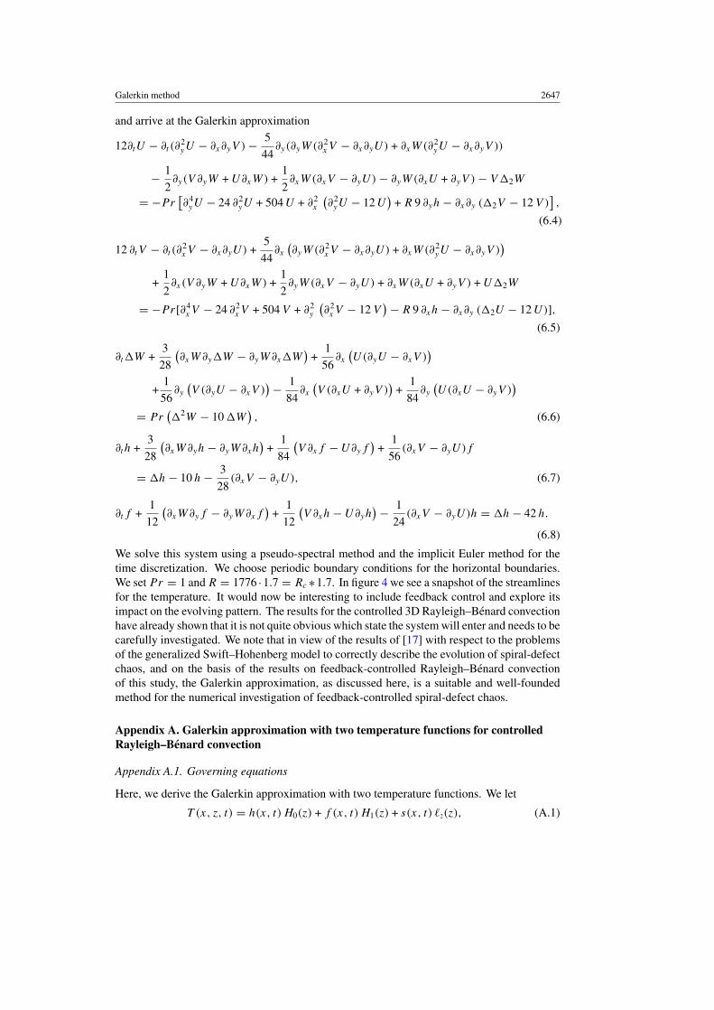
We solve this system using a pseudo-spectral method and the implicit Euler method for thetime discretization. We choose periodic boundary conditions for the horizontal boundaries.We set Pr = 1 and R = 1776 ·1.7 = Rc ∗1.7. In figure 4 we see a snapshot of the streamlinesfor the temperature. It would now be interesting to include feedback control and explore itsimpact on the evolving pattern. The results for the controlled 3D Rayleigh–Benard convectionhave already shown that it is not quite obvious which state the system will enter and needs to becarefully investigated. We note that in view of the results of [17] with respect to the problemsof the generalized Swift–Hohenberg model to correctly describe the evolution of spiral-defectchaos, and on the basis of the results on feedback-controlled Rayleigh–Benard convectionof this study, the Galerkin approximation, as discussed here, is a suitable and well-foundedmethod for the numerical investigation of feedback-controlled spiral-defect chaos.

Appendix A. Galerkin approximation with two temperature functions for controlledRayleigh–Benard convection

Appendix A.1. Governing equations

Here, we derive the Galerkin approximation with two temperature functions. We let

T (x, z, t) = h(x, t) H0(z) + f (x, t) H1(z) + s(x, t) �2(z), (A.1)

2648 A Munch and B Wagner

where H0(z) and H1(z) are chosen such that H0(1/2) = 0 and H ′0(−1/2) = 0 which yields a

second order polynomial, while the same conditions for H1(z) together with

〈H0, H1〉 = 0 (A.2)

yield a third order polynomial. We arrive at

H0(z) =(

z − 1

2

) (z +

3

2

), (A.3)

H1(z) =(

z − 1

2

) (z2 +

29

32z +

7

64

). (A.4)

The polynomial �2(z) naturally must satisfy �2(1/2) = 0. The order will be further increasedby requiring the boundary condition at z = −1/2 to be satisfied. However, when consideringthe possibility of negative gain ω < 0 we obtain artificial singularities, not present in the fullproblem, unless

ρ2 =∫ 1/2

−1/2�2(z) dz = 〈�2, H0〉

∫ 1/2

−1/2H0(z) dz + 〈�2, H1〉

∫ 1/2

−1/2H1(z) dz

is satisfied. Calculations can be further simplified, if we choose �2(z) to also be orthogonal toH0 and H1. As a consequence, we obtain a polynomial of fourth order such that ρ2 = 0 andnormalize it such that �′

2(−1/2) = 1. This yields

�2(z) = −7

4

(z − 1

2

) (z3 +

1

10z2 − 17

140z − 1

280

). (A.5)

For the velocity function we require u to be divergence free. Additionally, we require no-slipboundary conditions at z = 1/2 and z = −1/2. This yields

v(x, z, t) = u(x, t) µz(z), w(x, z, t) = −ux(x, t) µ(z), (A.6)

where

µ(z) = 1

4

(z2 − 1

4

)2

. (A.7)

We can now derive the Galerkin approximation by testing the full problem with the testfunctions

θ0 = δ(x) µz(z), θ1 = −δ′(x) µz(z), (A.8)

φ0 = δ(x)H0(z), φ1 = δ(x)H1(z), (A.9)

to obtain

uxxxx − 24 uxx + 504 u = −R

(60 h +

27

8f − 1

5s

)x

, (A.10)

ht − hxx +5

2h +

9

448

(hxu +

1

2hux

)= − 5

64f +

15

8s +

5

448ux

+1

448

(97

96fxu +

91

64f ux

)+

1

448 · 20

(3 sxu +

37

12sux

), (A.11)

ft − fxx +3059

130f − 173

390 · 32

(fxu +

1

2f ux

)= −112

13h − 6132

325s +

9

130ux

+1

390

(97 hxu − 79

2hux

)+

1

429 · 200

(31 sxu +

3 · 329

4sux

), (A.12)

Galerkin method 2649

with

s = ω

(2

3hxx +

1

48fxx

). (A.13)

Appendix A.2. Linear stability for two temperature functions

We first like to determine the critical Raleigh number (Rc) of the above problem. We linearizeabout the conductive state, hence about u(x, t) = 0, h(x, t) = 0, f (x, t) = 0 and s(x, t) = 0.

uxxxx − 24 uxx + 504 u = −R

(60 h +

27

8f − 1

5s

)x

, (A.14)

ht − hxx +5

2h = − 5

64f +

15

8s +

5

448ux, (A.15)

ft − fxx +3059

130f = −112

13h − 6132

325s +

9

130ux, (A.16)

with

s = ω

(2

3hxx +

1

48fxx

). (A.17)

Fourier transformation of the above equations yields

ht = −(

k2 +5

2

)h − 5

64f +

15

8s +

5

448i k u, (A.18)

ft = −(

k2 +3059

130

)f − 112

13h − 6132

325s +

9

130i k u, (A.19)

where

s = −ω k2

(2

3h +

1

48f

)and

i k u = M R

(60 h +

27

8f − 1

5s

)with M = k2

k4 + 24 k2 + 504,

with the solution of A.18–A.19

h(k, t) = K1 a1 exp(σ1 t) + K2 a2 exp(σ2 t), (A.20)

f (k, t) = K1 exp(σ1 t) + K2 exp(σ2 t), (A.21)

where K1 and K2 are constants and

a1 = 1

2D

(A − C +

√(A − C)2 + 4DB

), (A.22)

a2 = 1

2D

(A − C −

√(A − C)2 + 4DB

), (A.23)

σ1 = 1

2

(A + C +

√(A − C)2 + 4DB

), (A.24)

σ2 = 1

2

(A + C −

√(A − C)2 + 4DB

), (A.25)

2650 A Munch and B Wagner

with

A(k2, ω) = −k2 − 5

2+ R

5

448

(60 +

2

15ωk2

)M − 5

4ωk2, (A.26)

B(k2, ω) = R5

448

(27

8+

1

240ωk2

)M − 5

64− 5

128ωk2, (A.27)

C(k2, ω) = −k2 − 3059

130+ R

9

130

(27

8+

1

240ωk2

)M +

511

1300ωk2, (A.28)

D(k2, ω) = R9

130

(60 +

2

15ωk2

)M − 112

13+

4088

325ωk2. (A.29)

From this we calculate from the dominant growth rate σ1, by solving

σ1 = 0 and∂σ1

∂R= 0 (A.30)

the critical Rayleigh number Rac = 1350 together with the critical wavenumber kc = 2.52.

Acknowledgments

The authors thank Andrea Bertozzi for many fruitful discussions. They would also like to thankone of the anonymous referees for some very helpful comments. AM greatly appreciates thesupport from the DFG Heisenberg fellowship.

References

[1] Lord Rayleigh 1916 On convection currents in a horizontal layer of fluid, when the higher temperature is on theunder side Phil. Mag. 32 529–46

[2] Benard H 1901 Les tourbillons cellulaires dans une nappe liquide transportant de la chaleur par convection enregime permanent Ann. Chim. Phys. 23 62–144

[3] Busse F H 1967 The stability of finite amplitude cellular convection and its relation to an extremum principleJ. Fluid Mech. 30 625–649

[4] Clever R M and Busse F H 1974 Transition to time-dependent convection J. Fluid Mech. 65 625–45[5] Cross M C and Hohenberg P C 1993 Pattern formation outside of equilibrium Rev. Mod. Phys. 65 851–1112[6] Bodenschatz E, Pesch W and Ahlers G 2000 Recent developments in Rayleigh–Benard convection Ann. Rev.

Fluid Mech. 32 709–78[7] Manneville P 2006 Rayleigh–Benard Convection Thirty Years of Experimental, Theoretical, and Modeling Work

(Springer Tracts in Modern Physics vol 207) (Berlin: Springer) pp 41–65[8] Ahlers G and Behringer R P 1978 Evolution of turbulence from the Rayleigh–Benard instability Phys. Rev. Lett.

40 712–16[9] Greenside H S, Cross M C and Coughran W M Jr 1988 Mean flows and the onset of chaos in large-cell convection

Phys. Rev. Lett. 60 2269–72[10] Morris S W, Bodenschatz E, Cannell D S and Ahlers G 1993 Spiral defect chaos in large aspect ratio Rayleigh–

Benard convection Phys. Rev. Lett. 71 2026–9[11] Assenheimer M and Steinberg V 1993 Rayleigh–Benard convection near the gas–liquid critical point Phys. Rev.

Lett. 70 3888–91[12] Decker W, Pesch W and Weber A 1994 Spiral defect chaos in Rayleigh–Benard convection Phys. Rev. Lett.

73 648–51[13] Pesch W 1996 Complex spatiotemporal convection patterns Chaos 6 348–57[14] Xi H, Gunton J D and Vinals J 1993 Spiral defect chaos in a model of Rayleigh–Benard convection Phys. Rev.

Lett. 71 2030–3[15] Tu Y and Cross M C 1996 Defect dynamics for spiral chaos in Rayleigh–Benard convection Phys. Rev. Lett.

75 834–37[16] Bestehorn M, Fantz M and Haken H 1992 Spiral patterns in thermal convection Zeitschrift fur Physik B 88 93–4

Galerkin method 2651

[17] Schmitz R, Pesch W and Zimmermann W 2002 Spiral-defect chaos Swift–Hohenberg model versus Boussinesqequations Phys. Rev. E 65 037302–1

[18] Muller G 1988 Convection and inhomogeneities in crystal growth from the melt Crystals Growth, Properties,and Applications ed H C Freyhardt et al (Berlin: Springer)

[19] Tang J and Bau H H 1993 Stabilization of the no-motion state in Rayleigh–Benard convection through the useof feedback control Phys. Rev. Lett. 70 1795–8

[20] Tang J and Bau H H 1993 Feedback control stabilization of the no-motion state in a horizontal, porous layerheated from below J. Fluid Mech. 257 485–505

[21] Tang J and Bau H H 1998 Experiments on the stabilization of the no-motion state of a fluid layer heated frombelow and cooled from above J. Fluid Mech. 363 153–71

[22] Howle L E 1997 Control of Rayleigh–Benard convection in a small-aspect-ratio container Int. J. Heat MassTrans. 40 817–22

[23] Howle L E 1997 Active control of Rayleigh–Benard convection Phys. Fluids 9 1861–3[24] Howle L E 2000 The effect of boundary properties on controlled Rayleigh–Benard convection J. Fluid Mech.

411 39–58[25] Or A C, Cortelezzi L and Speyer J L 2001 Robust feedback control of Rayleigh–Benard convection J. Fluid

Mech. 437 175–202[26] Or A C and Speyer J L 2003 Active suppression of finite-amplitude Rayleigh–Benard convection J. Fluid Mech.

483 111–28[27] Or A C and Speyer J L 2005 Gain-scheduled controller for the suppression of convection at high Rayleigh

number Phys. Rev. E 71 046302[28] Remillieux M C, Zhao H and Bau H H 2007 Suppression of Rayleigh–Benard convection with proportional-

derivative controller Phys. Fluids 19 017102[29] Orszag S A and Thess A 1995 Surface-tension-driven Benard convection at infinite Prandtl number J. Fluid

Mech. 283 201–29[30] Howle L E 1997 Linear stability analysis of controlled Rayleigh–Benard convection using shadowgraphic

measurement Phys. Fluids 9 3111–3113[31] Wagner B A, Bertozzi A L and Howle L E 2003 Positive feedback control of Rayleigh–Benard convection

Discrete Cont. Dyn. B 3 619–42[32] Plaut E and Pesch W 1999 Extended weakly nonlinear theory of planar nematic convection Phys. Rev. E

59 1747–69[33] Manneville P 1983 A two-dimensional model for three-dimensional convective patterns in wide containers

J. Physique 4 759–65[34] Lagha M and Manneville P 2007 Modeling transitional plane Couette flow Eur. Phys. J. B 58 433–47[35] Ruyer-Quil C and Manneville P 2002 Further accuracy and convergence results on the modeling of flows down

inclined planes by weighted-residual approximations Phy. Fluids 14 170–83[36] Todd F Dupont and Hosoi A E 1998 Some reduced-dimension models based on numerical methods Modelling

and Computation for Applications in Mathematics, Science and Engineering (Oxford: Oxford UniversityPress) pp 59–80

[37] Skalicky T 1996 Laspack reference manual Version 1.12.3, Dresden University of Technology, Institute forFluid Mechanics

[38] Quateroni A and Canuto C 1982 Approximation results for orthogonal polynomials in Sobolev spaces Math.Comp. 38 67–86