Galactic Scale Dynamics in the External Field

Xufen Wu, HongSheng Zhao (University of St Andrews)

In collaboration with B. Famaey, G.Gentile, H.B.Perets, Y.G. Wang, C. Llinares, A. Knebe

Tully-Fisher relation and Rotation Curves of galaxies

(Milgrom 1983a,b,c; Bekenstein & Milgrom 1984; Sanders & McGaugh 2002)

Cosmic Microwave Background

Anisotropic Spectrum(Skordis et al. 2006)

g>>a0: µ=1, Newtong<<a0: µ=x, dMOND

a0 =1.2x10-10 m/s2

Structure Formation(Halle et al. 2007;

Skordis et al. 2008;Llinares et al. 2008)

Bullet Cluster(Angus et al. 2007; Llinares et al. 2009)

Tidal Dwarf Galaxies(Gentile et al. 2008)

Strong gravitational lenses(Zhao et al 2006; Chen & Zhao 2006,

Shan et al. 2008)

Weak Lensing(Angus et al. 2007;

Famaey et al. 2007)

Talk by Sanders / FamaeyTalk by Gentile

Talk by Angus / Llinares

Talk by Feix

Basic idea of MOND:

g>> : µ=1, Newtong<< : µ=x, dMOND

x =|∇Φ|a0

=g

a0

a0 = 1.2× 10−10m · s−2

∇ · [µ(x)∇Φ] = 4πGρ(BM 1984)

a0a0

MOdified Newtonian Dynamics

φ∞ ∝ log r =∞Milgrom (1983); Bekenstein & Milgrom

(1984);

The effective mass of dark matter is infinite for isolated systems !

dMOND:

µ -> 0 when r -> infinity

So we get Flat Vcir :), but not stars can escape!

Real System embedded in External Field:

Newtonian: ∆=0Deep MOND: ∆=1

yz

x

!gext

∆ =(

d lnµ

d lnX

)|X= |gext|

a0

x (kpc)

y (kpc)

Milky Way Potential contours

∇ · [µ(|g|a0

)g] = 4πGρ

g = gext −∇Φint

Φ∞int = − GM

µ(gext/a0)√

(1 +")(y2 + z2) + x2

The Correct Way

Axis Ratios of Potential At large radii (EF

dominated)the MONDian

potential axis ratio ~ 1/√2

yz

x

!gext

1√2

1

1

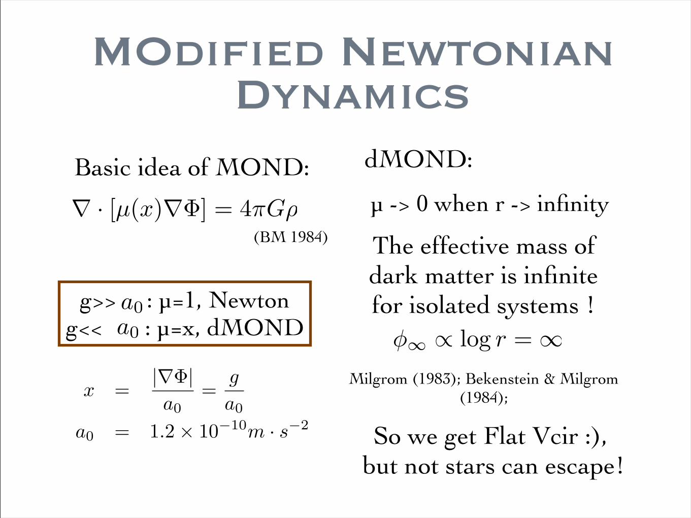
Phantom Dark Matter

Isodensity of phantom dark matter in a MOND MW embedded in an external field of 0.01a0 (panels a and b) and 0.03a0 (panels c and d). The dashed lines are negative isodensities and expected to observe such effects from lensing.

Wu et al. 2008

MOND predicts negative phantom dark matter at some regions when there’s EF.

ρ < 0

ρ > 0

To Escape ...

External Field !

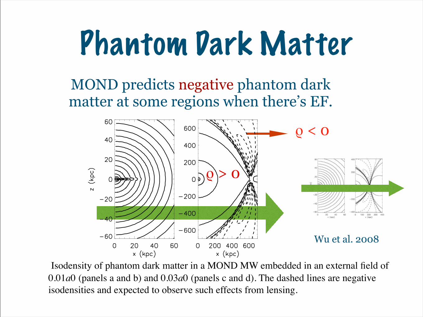
v2esc(x, y, z)

2+ Φint(x, y, z) ≡ Eeff = 0

Escape velocity is defined :

Weak External Field from Larger Scale Structure

Strong External Field from Rich Clusters of Galaxies

Great Attractor

Escape into backgrounds

EF of MW:

Wu et al. 2007

Famaey et al. 2006

∼ H0 × 600km/s ∼ 0.01+0.02−0.0075a0

Baryons for MOND and CDM (with NFW halo profile): Besançon Milky

Way Model (Robin et al. 2006)

if in clusters

if in field

External Fields

Dark Matter Halos

image from http://www.spacescan.org/page/4/image from http://space.newscientist.com/article/dn12646

image from http://www.ucolick.org/news/2006/index.html

Cold Dark Matter Halos

• MOND was thought to be unique while CDM has lots of models and parameters : isothermal model; Navarro-Frenk-White profile; Wilkinson & Evans profile; etc.

LMC is about to escape in CDM models.

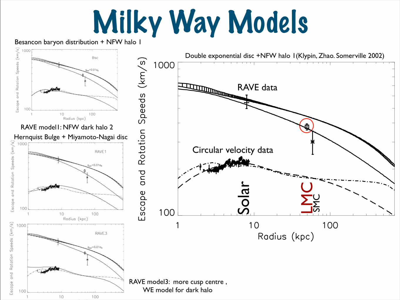
Double exponential disc +NFW halo 1(Klypin, Zhao. Somerville 2002)

Besancon baryon distribution + NFW halo 1

RAVE model1: NFW dark halo 2

RAVE model3: more cusp centre , WE model for dark halo

Hernquist Bulge + Miyamoto-Nagai disc

Sola

r

LMC

SMC

Milky Way Models

RAVE data

Circular velocity data

Table 2. Velocities and positions of Magellanic Clouds.

Parameters Radius (x, y, z)(kpc) |r|(kpc) 3D velocity (vx, vy, vz)(km s−1) |v|(km s−1)

LMC (−0.8, −41.5, −26.9) 49.5 (−86 ± 12, − 268 ± 11, 252 ± 16) 378 ± 18SMC (15.3, −36.9, −43.3) 58.9 (−87 ± 48, − 247 ± 42, 149 ± 37) 302 ± 52

Table 3. Observed 3D velocity and escape velocity at the position of the LMC (in units of km s−1).

Observation MOND (EF = 0.01a0) MOND (EF = 0.03a0) KZS Besancon RAVE1 RAVE3

378 ± 18 (441.8, 442.8, 442.0) (366.0, 367.8, 366.9) 368.9 366.9 348.6 375.7

LMC velocity is on the edge of escaping in CDM.

(Kallivayalil et al. 2006Besla et al. 2007)

Image from : http://apod.nasa.gov/apod/ap980826.html

Questions & Problems : 1. LMC-SMC system?2. Formation of Magellanic Stream?3. The orbital angular momentum of LMC ?

Will the LMC Escape?

New observational data of rotation curve from SDSS data (Xue et al. 2008)

image from http://www.daviddarling.info/encyclopedia/H/hypervelocity_star.html

A HVS is escaping from the Galaxy.

Observations of any incoming HyperVelocity Star would rule out CDM models! Perets, Wu et al 2008, arXiv:0809.2087

Prediction for HVS & SDSS Survey

In Newtonian Gravity, there exists instability on some models for galaxies

Can we find stable models for galaxies in MOND?

•Nbody Simulations:

density axis ratio a:b:c=1: 0.86 : 0.7 kpc

Constructing galaxies with Hernquist profile ,

i.e. 1/r cusp centreM87

NGC1316

ρ =M

2πabc

1r(r + 1)3

r =√(x

a

)2+

(y

b

)2+

(z

c

)2

(Wang et al. 2008, ApJ, 677, 1033; Wu et al. 2009, MNRAS, in press)

Triaxial Cuspy Galaxy Stability

Equilibrium model---------------------------

Stability

ρ =M

2πabc

1r(r + 1)3

∇ · [µ(x)∇Φ] = 4πGρ

Eq.1

Eq.2

µ(x) =x

1 + xEq.3

Eq.4 χ2 =1

Ncells

Ncells∑

i=1

Norbits∑

j=1

WjOij −Mi

2

nj = WjNtotalEq.5

Schwarzschild Technique+NMODY

The first octant is divided into 21 equal mass sectors by 20 shells.The first octant is further divided by planes z = cx/a, y = bx/a and z = cy/b (left panel) into 3 parts. Each part is subdivided by planes ay/bx = 1/5, 2/5, 2/3 and az /cx = 1/5, 2/5, 2/3 into 16 cells (right panel). we sub-divide the cells by the mid-planes of the cells once again.

1. Stationary Orbits:

Stationary orbits are launched from the central points of the outer shell surfaces of the sub-cells.

4 x 16 x (21-2) =192 orbits for each shell

Launch Orbits

2. x-z plane launched orbits:

Give a certain energy Ek = Φ(x, 0, z ) on Kth sector, Curve A is the minimal radius of 1:1 resonant orbits (x:y), and Curve B is the zero velocity surface. We define 10 lines satisfying x = z tan θ, where θ lies within the range 2.25◦ to 87.75◦ . Along the radial direction, we equally divide the radius between two boundaries into 16 parts with 15 points, where those 15 points are the initial positions for the orbits launched from the x − z plane.

There are 150 x − z plane starting orbits for each sector.

Launch Orbits

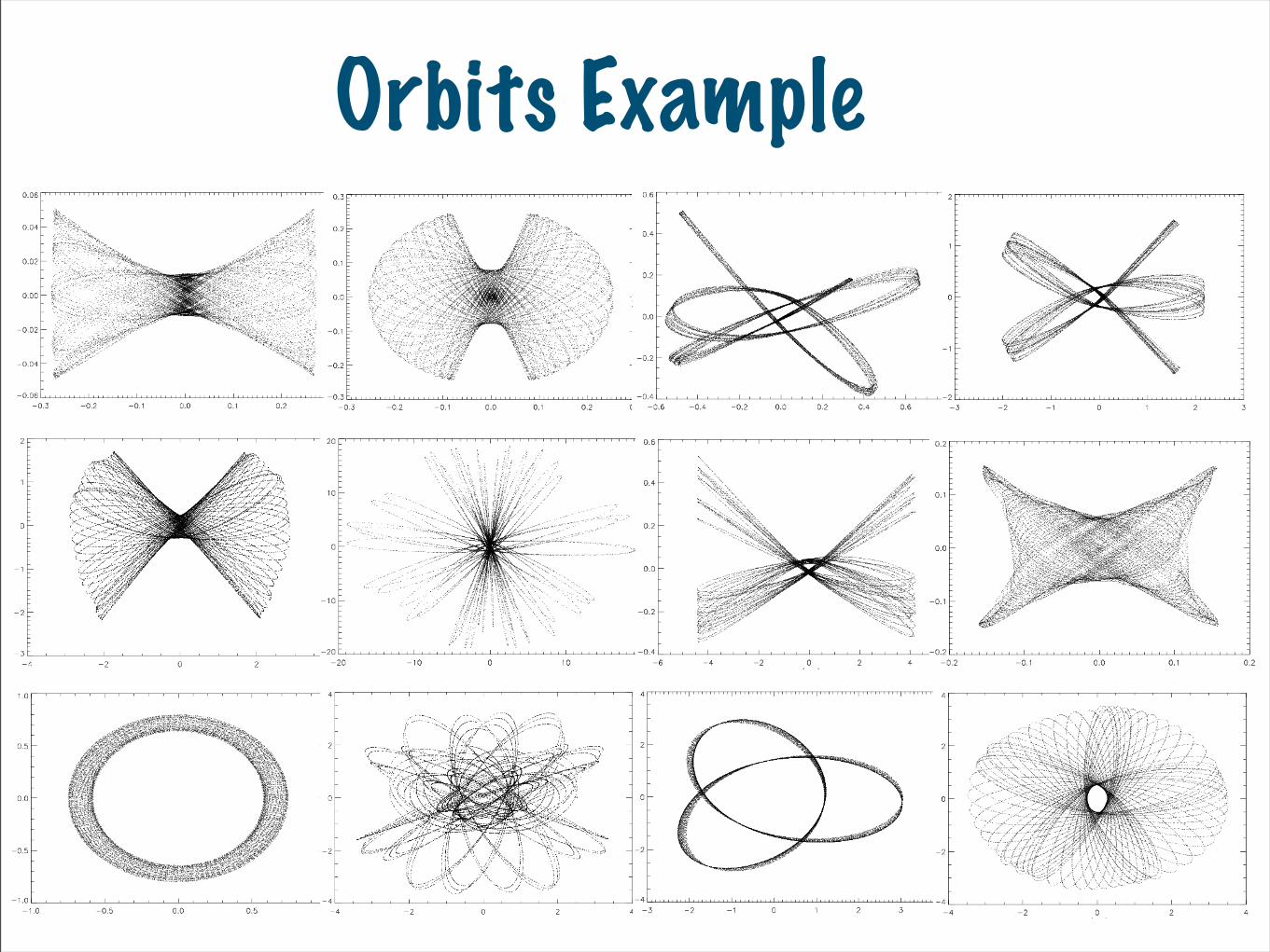
Orbits Example

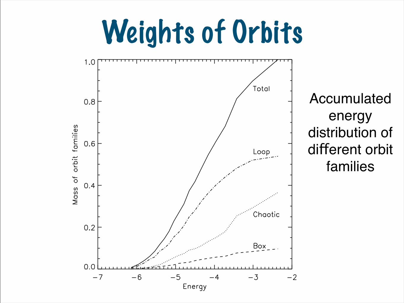
Accumulated energy

distribution of different orbit

families

Weights of Orbits

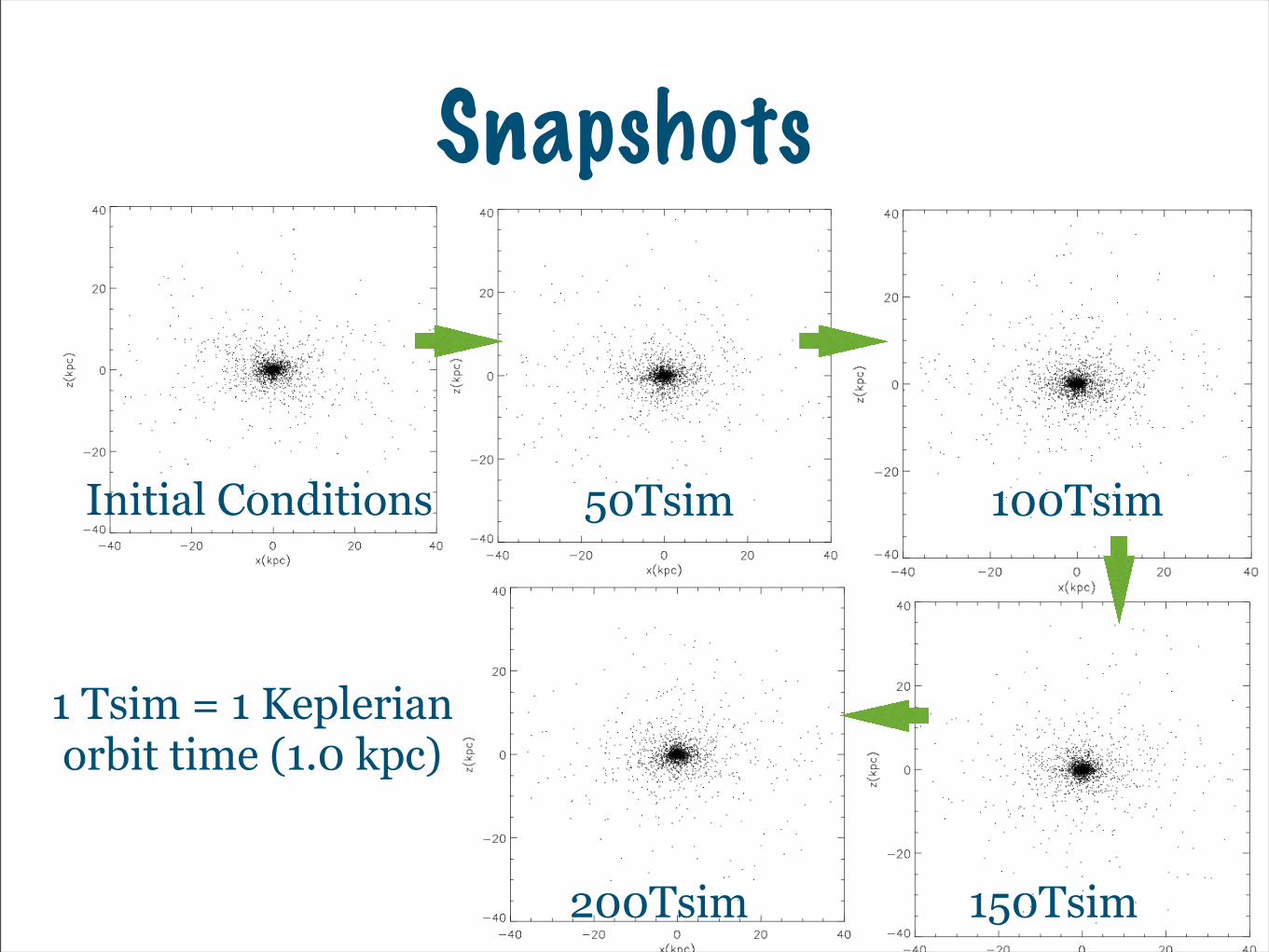
1 Tsim = 1 Keplerian orbit time (1.0 kpc)

50Tsim 100Tsim

150Tsim200Tsim

Initial Conditions

Snapshots

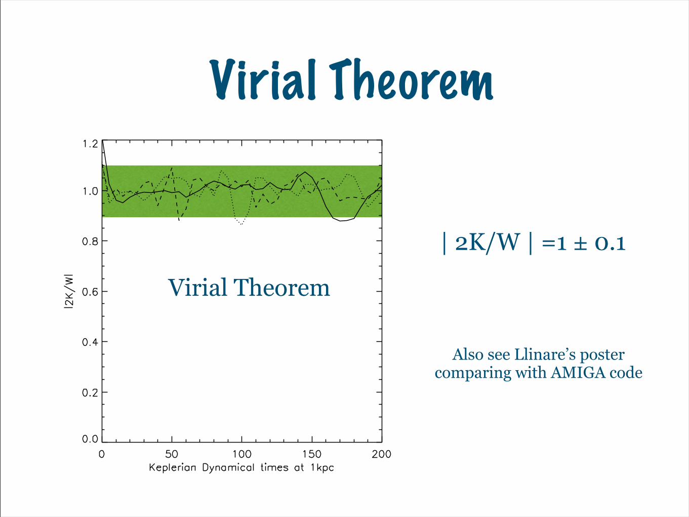
Virial Theorem

| 2K/W | =1 ± 0.1

Also see Llinare’s poster comparing with AMIGA code

Virial Theorem

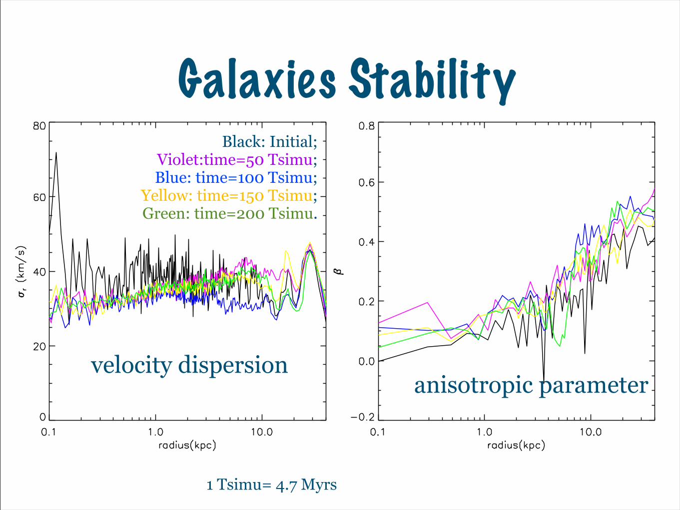
Galaxies StabilityBlack: Initial;

Violet:time=50 Tsimu; Blue: time=100 Tsimu;

Yellow: time=150 Tsimu; Green: time=200 Tsimu.

velocity dispersionanisotropic parameter

1 Tsimu= 4.7 Myrs

Galaxies Stability

Mass distribution

Black: Initial; Violet:time=50 Tsimu; Blue: time=100 Tsimu; Yellow: time=150 Tsimu; Green: time=200 Tsimu.

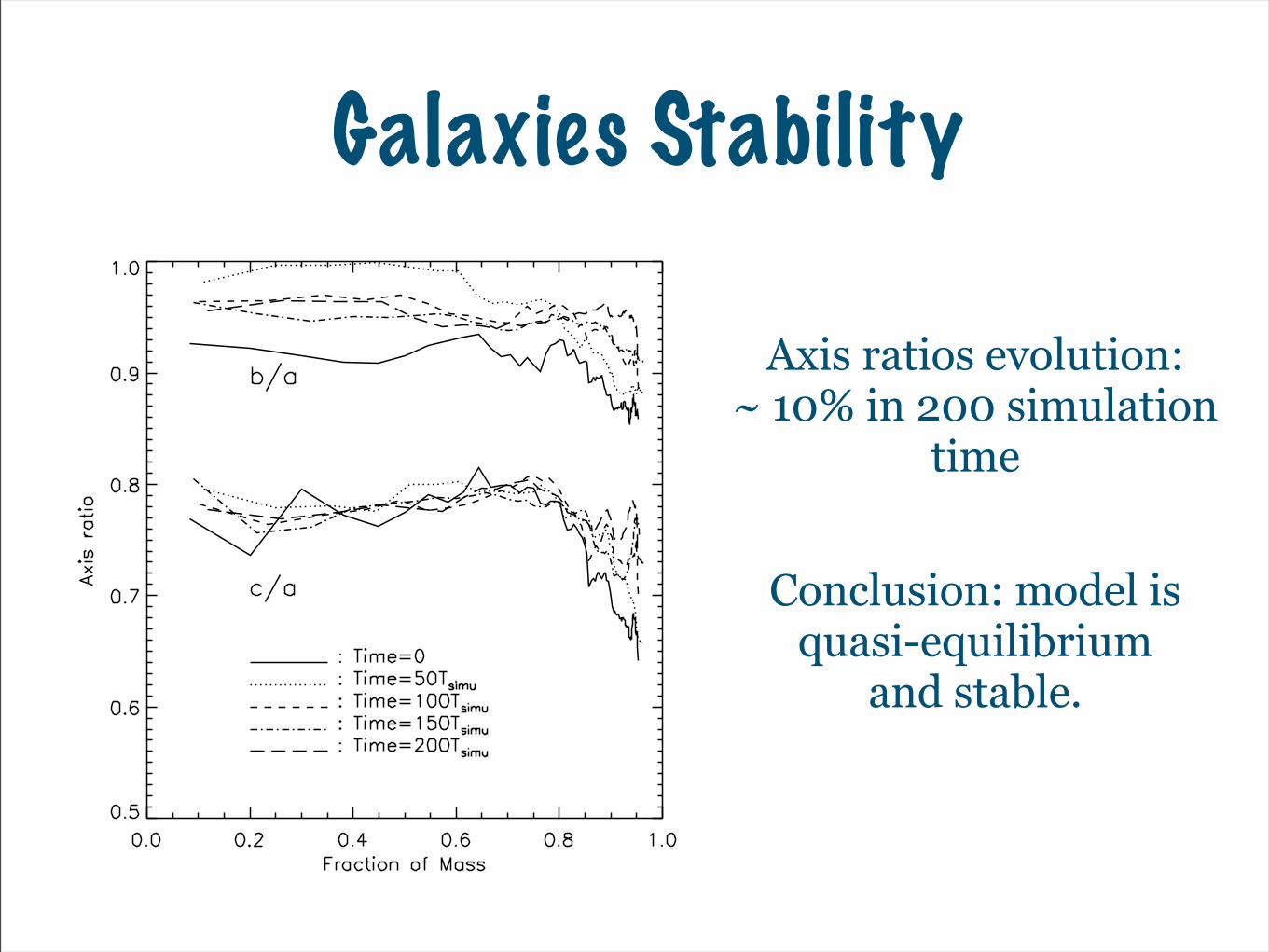
Galaxies Stability

Axis ratios evolution: ~ 10% in 200 simulation

time

Conclusion: model is quasi-equilibrium

and stable.

SummeryDisc galaxy:Galactic dynamics (LMC, HVS, RAVE, SDSS surveys) and lensing (negative density) could constrain theories: of dark matter halos and MOND.

Elliptical galaxy: There exist self-consistent galaxy models for elliptical galaxies in MOND.

On Going Work (MOND)1. Constructing triaxial galaxies Schwarzschild technique, fitting the data from observations. add external field : lopsided galaxies in rich clusters? 2. Testing self-consistency and stability (N-body) of the Milky Way bar 3. Galaxies merging existence of extremely elongated ellipticals? 4. Predicting lensing the negative convergence of gravitational lensing, i.e. the projected phantom dark matter density.

Thank You !