HAL Id: halshs-00641280https://halshs.archives-ouvertes.fr/halshs-00641280

Submitted on 15 Nov 2011

HAL is a multi-disciplinary open accessarchive for the deposit and dissemination of sci-entific research documents, whether they are pub-lished or not. The documents may come fromteaching and research institutions in France orabroad, or from public or private research centers.

L’archive ouverte pluridisciplinaire HAL, estdestinée au dépôt et à la diffusion de documentsscientifiques de niveau recherche, publiés ou non,émanant des établissements d’enseignement et derecherche français ou étrangers, des laboratoirespublics ou privés.

Cultural Proximity and TradeGabriel Felbermayr, Farid Toubal

To cite this version:Gabriel Felbermayr, Farid Toubal. Cultural Proximity and Trade. European Economic Review,Elsevier, 2010, 54, pp.279-293. �10.1016/j.euroecorev.2009.06.009�. �halshs-00641280�

Cultural Proximity and Trade ?

Gabriel J. Felbermayr a and Farid Toubal b

aDepartment of Economics, University of Hohenheim, GermanybUniversity of Angers, Paris School of Economics and CEPII, France

Abstract

Cultural proximity is an important determinant of bilateral trade volumes.However, empirical quantification and testing are difficult due to the elusive-ness of the concept and lack of observability. This paper draws on bilateralscore data from the Eurovision Song Contest, a very popular pan-Europeantelevision show, to construct a measure of cultural proximity which variesover time and within country pairs, and that correlates strongly with conven-tional indicators. Within the framework of a theory-grounded gravity model,we show that our measure positively affects trade volumes even if controllingfor standard measures of cultural proximity and bilateral fixed effects.

JEL classification: F12, F15, Z10

Keywords: International Trade, Gravity Equation, Cultural Proximity, Euro-

vision Song Contest.

? We are grateful for comments and suggestions from two anonymous referees, fromPhilippe Aghion, Keith Head, Raquel Fernandez, Victor Ginsburgh, Kala Krishna,Philippe Martin, Thierry Mayer, Peter Neary, John Romalis, and from seminarparticipants at the universities of Zurich, WHU-Otto Beisheim School of Manage-ment, Paris School of Economics, the annual meetings of the Canadian EconomicAssociation 2007 (Halifax), the EIIE 2007 (Ljubljana), the ETSG 2006 (Vienna)and the Verein fur Socialpolitik 2006 (Bayreuth). We are very grateful to JacquesMelitz for providing us with his detailed data on language. Part of this researchwas undertaken while Felbermayr was visiting Zurich University. Benny Jung andMichael Bohm have provided excellent research assistance. The usual disclaimerapplies.

Preprint submitted to Elsevier 19 May 2009

1 Introduction

There is wide-spread agreement that cultural proximity plays an important

role in determining trade flows between countries. The literature has used

different variables to proxy cultural ties, such as common language, religion,

or ethnicity (Boisso and Ferrantino, 1997; Frankel, 1997; Melitz, 2008). 1 While

those variables clearly capture cultural proximity, they also reflect other trade-

creating factors, such as the cost of communication.

In this paper, we exploit an original data set that contains information on cul-

tural proximity between European countries. Each year in May, the European

Broadcasting Union organizes the Eurovision Song Contest (ESC). This is a

huge pan-European televised show, where every participating country sends

an artist to perform a song. The other countries grade those songs, either

by televoting, or (in earlier times) by popular juries. Every year, the process

gives rise to a matrix of bilateral votes. Recent research shows that bilateral

votes are strongly affected by conventional measures of cultural proximity,

such as linguistic, ethnic, or religious ties (Ginsburgh and Noury, 2008; Gins-

burgh, 2005; Clerides and Stengos, 2006). However, in contrast to standard

indicators, the ESC scores vary over time and are potentially asymmetric.

ESC scores are informative about a broader concept of cultural proximity that

is close to the definition used by sociologists (Straubhaar, 2002). Cultural prox-

imity relates to the sharing of a common identity, to the feeling of belonging

to the same group, and to the degree of affinity between two countries. The

sociological concept allows for the evolution of bilateral attitudes and moods

over time and for asymmetries within pairs of countries. A country’s citizens

can display respect and sympathy for the cultural, societal, and technological

achievements of another country without this feeling necessarily being recip-

1 Other recent examples include Alesina and Dollar (2000), who use cultural prox-imity measures in the context of explaining international aid, and Rose (2004), whostudies the effect of WTO membership on trade. In Rauch and Trindade (2002) andCombes et al. (2005) cultural proximity is measured by the importance of ethnicties across countries or regions. There is also a growing literature that correlatesattitudes, sentiments, or customary beliefs to bilateral trade (Disdier and Mayer,2005; Guiso, et al., 2004). Disdier et al. (2007) use bilateral trade in cultural goodsas a proxy for cultural proximity.

1

rocal and ever-lasting. Conventional measures of cultural proximity, such as

common language, ethnicity, genetic traits, or religion are both time-invariant

(pre-determined) and, by construction, symmetric and can therefore not fully

capture the broad notion of cultural proximity.

Our interpretation of ESC scores is in line with anecdotal and systematic

evidence on voting patterns across and within country pairs and over time.

We show that some countries systematically award scores above average to

each other and behave in a reciprocal way. We detect a Nordic, a Balkan, and

a Mediterranean cluster. However, the observed degree of reciprocity can be

low even between countries of seemingly similar cultural attributes, and the

average degree of reciprocity is rather small.

Accounting for the unobserved quality of songs by including song-specific

dummy variables, we discover a statistically significant and economically mean-

ingful relation between bilateral ESC scores and the volume of trade between

two countries. Looking at trade in differentiated goods, moving from the lowest

to the highest degree of cultural proximity increases bilateral trade on aver-

age by 16% in our benchmark regressions. However, when considering trade

in homogeneous goods, which are typically traded on organized exchanges,

ESC scores are unrelated to bilateral trade volumes, signaling the irrelevance

of cultural proximity for promoting trade in that category of goods. Inter-

estingly, however, measures such as common language, common legal system,

or ethnic ties do turn out statistically significant. Since there is little reason

why cultural proximity should foster transactions taking place on anonymous

organized exchanges, we take this finding as evidence that ESC scores strictly

reflect cultural proximity while those other measures have more to do with

other trade-promoting channels, such as the pure costs of translation or con-

tracting.

The time-varying and asymmetric nature of ESC scores allows for a more

elaborate econometric treatment. We can exploit the time dimension in order

to deal with the potential endogeneity of grading behavior, to correct for non-

systematic measurement error in our index of cultural proximity or in order

to control for time-invariant unobserved factors that drive both cultural prox-

2

imity and bilateral trade. Following Baier and Bergstrand (2007), we include

dyad-specific fixed effects to control for those initial conditions, thereby nudg-

ing our results nearer to the true causal effect of cultural proximity on trade.

Our results suggest that cultural proximity increases bilateral trade by about

1.2% for differentiated goods, while, as before, it does not increase trade in

goods transacted over organized exchanges. Using time lags as instruments, we

find that OLS models also strongly underestimate the effect of cultural prox-

imity on trade, probably due to the presence of measurement error. Hence, the

central conclusion of our paper is that cultural proximity is a more important

determinant of bilateral trade than researchers usually allow with the sort of

cultural variables they include.

Our paper is related to different strands of the empirical gravity literature. We

frame our analysis in a monopolistic competition trade model close to Combes

et al. (2005), where an asymmetric weighting term in the utility function

allows cultural proximity to affect preferences. The other channel through

which cultural proximity matters is through trade costs. Our econometric

setup follows Baldagi et al. (2003) and Baier and Bergstrand (2007), who

include complete sets of interaction terms of importer/exporter dummies with

year fixed effects into the gravity model. This strategy is a natural extension

of the fixed effects approach discussed by Feenstra (2004). It appropriately

controls for multilateral resistance (Anderson and van Wincoop, 2003) and

other sorts of unobserved country-specific heterogeneity.

The received literature acknowledges the importance of the trade-cost and the

preference channels; see Combes et al. (2005). However, that paper deals with

migration and business networks; our exercise is related to a broader notion

of cultural proximity. There are two interesting papers which show that dis-

tance captures more than transportation costs. Huang (2007) disentangles the

distance effect of trade into a transport-cost and an unfamiliarity component.

Blum and Goldfarb (2006) show that distance matters even for services that

are entirely transacted over the internet and relate this finding to a preference

effect. Our paper differs as it focuses on cultural proximity (not geographical

distance), tries to explain patterns in trade in manufactures across Europe

3

and pays due attention to endogeneity and identification concerns. 2

The remainder of this paper is structured as follows. Section 2 provides a

thorough discussion of the data and shows how one can use ESC scores to

construct a meaningful measure of cultural proximity. Section 3 derives a

generalized theoretical trade flow equation, which highlights the role of cultural

proximity and which can be applied to bilateral data. Section 4 contains our

core empirical results and shows how ESC scores are related to bilateral trade.

Section 5 provides a number of extensions: it shows that our results are not

driven by possible endogeneity of the ESC scores or unobserved heterogeneity.

Section 6 concludes. Additional material and robustness checks can be found

in our working paper as well as in a web appendix. 3

2 Eurovision Song Contest score data

In this section, we discuss our data and show that the ESC scores are a

meaningful measure of cultural proximity. We also discuss their statistical

properties.

2.1 The setup of the contest and measurement issues

In 1955, a couple of European broadcasting stations represented in the Euro-

pean Broadcasting Union (EBU) founded the Eurovision Song Contest (ESC).

A year later, the first contest took place in Lugano, Switzerland. The idea of

the ESC is that each participating country selects an artist or a group of

artists to perform a song, which is then graded by the other countries.

We focus on the period 1975-2003, in which grading rules have been stable. 4

2 There is also a growing literature on the relation between culture and economicoutcomes; see Fernandez (2007) or Guiso et al. (2006) for comprehensive surveys,and Spolaore and Wacziarg (2009), Giuliano et al. (2006), Algan and Cahuc (2007)and Tabellini (2007) for interesting recent papers.

3 The web appendix can be downloaded fromhttp://team.univ-paris1.fr/teamperso/toubal/papers/CP/CP.html.

4

On average, from 1975 to 2003, 21.6 countries participated in the ESC, with

the minimum participation being 18 countries. Contest participants are almost

exclusively European countries. 5 Each ESC is broadcast by television, and

since 1985, this happens via satellite. In 2005, the contest was broadcast live

in over 40 countries to over 100 million spectators. Until 1988, the scores were

decided upon by a jury that is not necessarily consisting of experts. Nowadays,

the scores are national averages obtained through a televoting process with

huge popular participation. There are organizations of ESC fans in all EU

countries.

Since 1975, each country scores the other countries’ performances on a scale

from 0 to 12. The scores 9 and 11 are not allowed and 12 is the highest possible

score. Each of the ten strictly positive grades has to be allocated exactly once;

remaining countries are graded zero. The winner is the country that collects

the largest sum of points.

We argue that ESC scores are broad indicators of cultural proximity. However,

this interpretation poses one major difficulty, since the scores may reflect the

quality of the song. Thus, we assume that country i′s support for country

j′s performance at time t, ESCijt depends positively on the quality of the

song, ζjt, on the degree of country i′s feeling of cultural proximity towards j

at time t, Πijt. In addition, the rules of the song contest disallow ties for the 10

most popular songs and force ties for the least popular ones. There is therefore

no ordering of ESC scores below the top ten songs. Consequently, a separate

dummy variable, Dijt, is also appropriate for values of ESC equal 0 when

Dijt equal 1. Accordingly, ESCijt = f(Πijt, ζjt, Dijt

). Correspondingly we

may say

Πijt = f−1 (ESCijt, ζjt, Dijt) . (1)

Πijt refers here to cultural proximity as it emerges from the song contest

alone. We shall reserve the term Πijt for cultural proximity based onother

indicators as well.

4 Until 2003, the last year in our sample, the contest was organized in a single round.From 2004 onwards, there are two rounds to accommodate the rising number ofparticipants.

5 Israel participates on a regular basis and Morocco has participated once. Bothcountries are not in our sample.

5

2.2 ESC scores as broad indicators of cultural proximity

In this subsection, we show that ESC scores reflect time-invariant components

of cultural proximity. We also argue that their time and within country-pair

variance are in a meaningful way related to the broad definition of cultural

proximity discussed in the introduction.

Ginsburgh (2005) shows that conventional measures of cultural proximity –

linguistic, ethnic, religious, political, etc. ties – determine ESC outcomes to a

large extent, refuting the alternative hypothesis of vote trading (logrolling).

Clerides and Stengos (2006) and Spierdijk and Vellekoop (2008) similarly doc-

ument the importance of culture for scoring outcomes. Haan, Dijkstra, and

Dijkstra (2005) test whether the transition of the grading process from jury-

based voting to generalized televoting has strengthened the role of cultural

proximity and answer this question in the affirmative. Fenn et al. (2006) run a

cluster analysis and find evidence for unofficial cliques of countries along lines

of cultural proximity. 6

Table 1 shows pairwise correlation coefficients between raw and quality-adjusted

ESC scores, on the one hand and conventional measures of cultural proximity

Πijt (excluded from Πijt) on the other. We have rescaled the ESC scores so

that ESCijt ∈ [0, 1] to facilitate comparison with conventional measures of

cultural proximity. 7 The quality-adjusted ESC scores are the residuals from

a regression of raw scores on song-dummies. We consider the following time-

invariant and symmetric measures of cultural proximity used in the literature:

(i) an adjacency dummy and geographical distance between main cities (in

kilometers); (ii) the Melitz (2008) measures of common language, namely; the

continuous direct communication variable and the open-circuit communica-

tion dummy variable; 8 (iii) a dummy for common legal origin borrowed from

6 See also Yair (1995) for an early study of that sort.7 First, the original score of 10 is set to 9 and the score 12 is set to 10. Then, wedivide all scores by 10. This rescaling does not affect our results.

6

La Porta et al. (1999) 9 ; (iv) a continuous religious proximity measure based

on Alesina et al. (2000); (v) a measure of ethnic links based on the stock of

individuals born in country i but residing in country j; Appendix A provides

information on the summary statistics of the variables, their exact definition

and the data sources.

Table 1Coefficients of correlation between different measures of cultural proximity

ESC score Adjusted ESC scoreAdjusted ESC score1 0.8003***Geographical distance -0.1918*** -0.2528***Adjacency 0.1839*** 0.2203***Direct communication 0.1421*** 0.1341***Open-circuit communication 0.1633*** 0.1861***Common legal origin 0.1244*** 0.2111***Religious proximity 0.1317*** 0.1669***Ethnic links 0.3245*** 0.1968***1 averaged across years.Number of observations: 901. *** denotes that coefficient isdifferent from zero at 1% level of significance

The correlation between the quality adjusted ESC score and the raw ESC

score data is 80.03. Hence, about a fifth of the variance in raw scores is ac-

counted for by quality. The correlation coefficient between both ESC score

measures and the conventional proxies of cultural and geographical proximity

all have the right sign and are statistically different from zero. The adjusted

ESC score displays larger correlation coefficients (with the exceptions of direct

communication and ethnic links), signaling that quality adjustment improves

our index of cultural proximity.

8 Melitz (2008) distinguishes whether ease of communication facilitates tradethrough translation or the ability to communicate directly (i.e., face-to-face). Thefirst possibility is captured by the open circuit communication dummy, which takesvalue one if the language is either official or widely spoken (20% of the population)in both countries (in any combination). The second possibility is captured by adirect communication measure which obtains by summing up the products of therespective percentages of speakers over all the relevant languages (at least 4%) inthe two trading countries.

9 Countries that once were part of the same larger political entity (such as, e.g.,the Czech Republic and Hungary in the Austro-Hungarian Empire, England andIreland, or Norway and Denmark) usually have the same legal system. Hence, thatdummy also captures the broad institutional similarity of countries that have hada common past.

7

Table 2Explaining grading behavior

Poisson ZeroInflatedPart

Ln Distance -0.150*** 0.011(0.041) (0.093)

Adjacency -0.162* 0.010(0.087) (0.207)

Both country in same FTA -0.033 -0.038(0.041) (0.092)

Direct communication -0.230 -0.020(0.145) (0.474)

Open-circuit communication 0.333* -0.116(0.191) (0.448)

Common legal origin 0.147** -0.004(0.058) (0.129)

Religious proximity 0.248** 0.032(0.101) (0.211)

Ethnic ties 0.057*** 0.024(0.017) (0.019)

Observations 10,560Nonzero obs. 5,135Zero obs. 5,425McFadden’s adjusted R2 0.018Log-Likelihood Full Model -5,919.429Vuong Test: Zip vs. Standard Poisson 15.80***The regression contains song dummies and year fixed effects.Standard errors (in brackets) have been adjusted for clusteringaround country pairs. *,**,*** denote statistical significance atthe 10, 5, and 1 percent levels, respectively.

In Table 2, we present the results of a simple regression of ESC scores on

various measures of cultural proximity. In order to account for song quality

(ζjt) we include song dummies that are country-specific; moreover, the equa-

tion also contains year effects. Since we observe the same country pair over

several years, we adjust the standard errors for clustering. ESC scores are

count data censored at zero, so that it is natural to estimate a zero-inflated

Poisson model. 10 Indeed, the Vuong statistic indicates that this model has a

better fit than the standard Poisson model. Interestingly, while all measures

are strongly related to ESC scores in pairwise correlations, the multivariate

10 See Greene (2008, pp. 930-931) for a textbook treatment of the zero-inflatedPoisson model and further references.

8

analysis shows that direct communication does not matter for grading behav-

ior. However, the other variables related to cultural proximity replicate the

findings of table 1. Note that none of the measures explains the zero-inflated

part of the Poisson regression.

Table 3 shows that culturally close countries tend to award each other grades

above the average. But the degree of reciprocity is not very high, revealing

important within-pair variance. Table 3 reports the directed pair-specific in-

tercepts νij derived from estimating ESCijt = ψjt + ξij + uijt by OLS, where

ψjt is the average score attained by country j at time t and uijt is an error

term. We refer to the empirical estimates of the intercepts ξij as excessij since

they measure the excess of the average (over time) score that i allows to j

relative to the overall average (over all countries and time) that j receives.

Table 3 shows selected country relations where excess-grading is statistically

significant at least in one direction. 11 The expected country clustering read-

ily emerges. For example, Cyprus awards to Greece an average of 7.41 points

more than Greece receives on average; Greece reciprocates by awarding an

excess of 6.26 points beyond the Cypriot mean score. Over-generous and re-

ciprocal relationships can be found for many Scandinavian country pairs, and

to a lesser extent for Mediterranean countries. However, relationships need not

be reciprocal: Finland awards Italy an excess 3.10 points, but gets an aver-

age negative excess grade of -0.77 in return. France grades Great Britain 0.86

points below average, while the Brits treat France almost neutrally. 12 Scandi-

navian and Mediterranean countries tend to reciprocally award scores below

the respective averages (with the pair Denmark-Yugoslavia the notable excep-

tion). Not surprisingly, Cyprus and Turkey stand out as two countries that

systematically award each other grades below average. Germany (and Austria)

over-grade Turkey without being compensated; this is likely to reflect ethnic

ties due to migration.

Table 3 reveals an intuitive pattern. Reciprocal positive excess grades occur

within culturally close pairs; reciprocal negative excess grades appear for the

11 See also Table 1 in Clerides and Stengos (2006).12 This confirms the Duke of Wellington: “We always have been, we are, and I hopethat we always shall be detested in France. ” (cited by Guiso et al., 2007, p. 1.).

9

Table 3ESC scores: Selected deviations from means

Country i Country j excessij std. err. excessji std. err.CYP GRC 7.41 0.65 6.26 0.65ITA PRT 3.95 0.63 0.02 0.63DNK ISL 3.27 0.72 2.05 0.72FIN ITA 3.10 0.65 -0.77 0.65DNK SWE 2.99 0.55 1.98 0.55ISL SWE 2.95 0.65 1.56 0.65ESP ITA 2.95 0.63 1.70 0.63CYP YUG 2.67 0.82 2.49 0.82HRV MLT 2.52 0.78 3.17 0.78TUR YUG 2.22 0.75 3.21 0.75DNK NOR 2.04 0.57 0.79 0.57GER TUR 1.79 0.53 -0.70 0.53CYP ESP 1.79 0.57 -0.27 0.57ESP GRC 1.77 0.54 2.62 0.54ISL NOR 1.71 0.65 1.08 0.65NOR SWE 1.56 0.50 2.64 0.50BEL NLD 1.33 0.55 0.30 0.55AUT TUR 1.12 0.55 -0.21 0.55FIN SWE 1.06 0.54 0.67 0.54FRA GBR -0.86 0.49 0.18 0.49ESP NOR -1.01 0.49 -1.37 0.49ESP SWE -1.39 0.49 -1.20 0.49ITA SWE -1.51 0.65 -0.93 0.65DNK ESP -1.66 0.55 -0.39 0.55ISR ITA -1.73 0.69 -1.73 0.69HRV SWE -1.76 0.78 -3.06 0.78DNK HRV -1.92 0.98 -2.53 0.98CYP TUR -2.09 0.58 -1.22 0.58DNK YUG -2.17 0.78 1.34 0.78Pair-specific intercepts, means adjusted. All estimates are significant at10 percent level. All country pairs in the table occur at least 10 timesin the data. Excessij denotes the score awarded by i to j in excess toj’s average score.

usual suspects but are on average smaller than positive excess grades. More-

over, non-reciprocal behavior seems to be quite frequent. The (simple) corre-

lation coefficient between excessij and excessji is 35.07, the Spearman rank

correlation coefficient is 27.81; both measures are statistically different from

zero at the one percent level of significance.

There is plenty of anecdotal evidence that ESC scores reflect changes in atti-

10

tudes and moods over time. For example, The Economist described the victory

of Serbia in 2003 and that of Turkey in 2007 as signs that the other Euro-

pean countries perceive Serbia and Turkey as less culturally remote (May

29, 2003; May 17, 2007). The successes of Estonia and Latvia in 2001 and

2002, respectively, received similar comment (May 30, 2002). The success of

Finland in 2006 was associated to the widespread perception of a successful

‘Finnish model’ (July 6, 2006). According to long-time commentator Terry

Wogan from the BBC, the failure of Britain to earn a single point in 2003 was

due to Britain’s decision to back the United States in its attack on Iraq. 13

While the examples cited above mark short-term effects, the data also reveals

long-run trends. For example, the popularity of countries seems subject to

cycles that are difficult to reconcile with underlying movements in musical

quality. For example, The Economist relates the failure of France to win any

contest since 1977 to the loss of French popularity and cultural clout in Europe

(May 12, 2005). The example of Italy offers a similar, but less spectacular,

picture. It is well possible that the popularity of Celtic culture (Ireland) will

suffer the same fate. 14

Gatherer (2006) provides systematic evidence for time shifts in bilateral popu-

larity. He simulates matrices of ‘unbiased’ ESC score outcomes and compares

them to actual voting. He shows that collusive voting alliances, described by

several authors (e.g., Fenn et al., 2005) have shifted over time. The observed

time pattern makes sense: France has lost its early central role to English-

speaking countries (Ireland, Britain), which have then given way to Eastern

Europe.

13 BBC News “Turkish delight at Eurovision win”, Saturday 24 May 2003. More-over, while all those effects naturally have a country-time dimension, their receptionacross Europe and hence their importance for bilateral trade need not be identical.

14 Figure 1 in the web appendix presents the time profile of multilateral unadjustedESC scores earned by frequently participating countries.

11

3 Cultural proximity in the gravity model

We base our theoretical model on the multi-country monopolistic competi-

tion model of trade (see Feenstra, 2004, for an overview). Each country i is

populated by a representative individual who derives utility from consum-

ing different varieties of a differentiated good according to a standard CES

function,

Uit =C∑j=1

aσ−1σ

ijt

njt∑z=1

(mzijt)σ−1σ , (2)

where z denotes the index of a generic variety, njt is the number of varieties

produced in country j at time t and σ > 1 is the elasticity of substitution

between varieties. The quantity of consumption in country i of variety z from

country j ismzijt. Following Combes et al. (2005), we allow for a specific weight

aijt ≥ 0 to describe the special preference of the representative consumer in

country i for goods from country j.

All varieties from the same origin bear the same f.o.b. (ex factory) price pjt

(reflecting symmetric production technologies), and iceberg ad-valorem trade

costs payable for deliveries from j to i, tijt ≥ 1, do not depend on the charac-

teristics of the varieties within a sector. Hence, the c.i.f. price (i.e., including

trade costs) paid by consumers pijt = pjttijt is the same for all varieties im-

ported from j. It follows that consumed quantities mzijt are identical for all z

so that we can omit the variety index in the sequel.

Maximizing (2) subject to an appropriate budget constraint, one derives coun-

try i′s demand quantity mijt for a generic variety. Calculating the c.i.f. value

of total imports from country j at time t as Mijt = njtpijtmijt, we find 15

Mijt =

(aijttijt

)σ−1

µitφjt. (3)

The variables µit ≡ EitPσ−1it and φjt ≡ njtp

1−σjt collect terms that depend only

on country i′s or j′s characteristics. Pit =[∑C

j=1

(aijttijt

)σ−1p1−σjt njt

] 11−σ

is the

15 Note that Combes (2007) express imports in terms of quantities not values.

12

aggregate price index and Eit denotes country i′s GDP.

For our empirical investigation, we do not need to close the model by explic-

itly specifying supply-side and equilibrium conditions. However, we need to

clarify the role of cultural proximity in shaping bilateral trade flows. Cultural

proximity affects the bilateral trade equation (3) in two ways. On the one

hand, it lowers trade costs, tijt: a higher total level of trust, the easier forma-

tion of business and/or social networks, or fewer misunderstandings related to

non-verbal communication make expensive hedging measures and consulting

services redundant. This is the trade-cost channel of cultural proximity. On

the other hand, cultural proximity is also reflected in the bilateral affinity pa-

rameter aijt. A high value of aijt means that the representative consumer in

country i puts a high value on products produced in country j. Equation 3

together with the assumption σ > 1 implies that this situation leads to larger

trade volumes. This is the preference channel of cultural proximity.

In our empirical set up, as indicated earlier, we capture cultural proximity

Πijt by the revealed degree of cultural proximity (quality adjusted) obtained

from the ESC, Πijt, and by the more conventional measures, discussed in

section 2.2, such as linguistic proximity, direct communication DCij, and open

circuit communication OCij, the existence of common legal origins (LAWij),

the intensity of ethnic ties (log of bilateral migrant stock, ETHij), and the

degree of religious proximity (RELij) . Grouping the conventional indicators

into the vector Kij, we posit

Πijt = Πijt + κ′ ·Kij (4)

where κ is a (column) vector of parameters. In principle, all components of

K may be time-varying. However, there is only cross-sectional information

available on these variables. Hence, the ESC scores are the only source of

time-variant information about time-varying cultural proximity.

We now specify how country i′s cultural proximity to country j is related to

bilateral affinity and trade costs. We assume that country i′s preference for

13

goods from j, aijt, depends on cultural proximity Πijt in the following way:

ln aijt = αΠijt, (5)

where α > 0. Similarly, we assume that trade costs tijt also depend on Πijt.

However, besides cultural proximity, there are at least three other fundamental

determinants of trade costs: 16 (i) Transportation costs, reflected by geograph-

ical distance (DISTij) and the existence of a common land border (adjacency,

dummy variable ADJij); (ii) formal trade policy, measured by joint member-

ship in a free trade agreement (dummy variable FTAijt); and (iii) costs of

contracting and negotiation. The latter category is closely related to cultural

proximity since higher trust and understanding amongst parties certainly low-

ers transaction costs. However, transaction costs can be low for reasons un-

related to cultural proximity, e.g., if a common legal system facilitates the

write-up of contracts or if citizens in both countries master the language of

some third country. We write iceberg trade costs as

ln tijt = δ lnDISTij − γADJij − ϕFTAijt − πΠijt. (6)

We expect that all parameters δ, γ, ϕ and π are positive.

Using a linearized version of the ESC score equation (1), together with equa-

tions (4), (5) and (6) in (3), we obtain the following log-linear gravity equation:

lnMijt = ηESCijt+κ1DCij + κ2OCij + κ3LAWij + κ4ETHij + κ5RELij

−δ lnDISTij + γADJij + ϕFTAijt+νit + νjt +Dijt + εijt, (7)

where η ≡ (σ − 1) (α + π) , κk = ηκk and κk being the coefficients associated

to each element in the vector Kij, δ ≡ (σ − 1) δ, γ ≡ (σ − 1) γ, ϕ ≡ (σ − 1)ϕ,

and εijt ≡ (1− σ) (α + π)uijt. The vectors νit and νjt collect importer × year

and exporter × year fixed effects to control for µit, and φjt (both of which have

important unobserved components such as the true price index, the number

of firms, or the price of a generic variety) as well as for song quality. Finally,

16 See Anderson and van Wincoop (2004) for a classification of different types oftrade costs.

14

εijt is the error term. The use of fixed effects makes the inclusion of GDP or

price data redundant. It also frees us from the need to think about the choice

of proper deflators for right and left-hand side variables of the gravity equa-

tion. 17 Equation (7) contains only pair-specific variables, because country-

specific ones are perfectly controlled for by country-specific fixed effects. 18

Our main parameters of interest are η and the coefficients of the more standard

measures of cultural proximity κ1 to κ4. These coefficients reflect both the

trade cost (through π) and the preference channel (through α).

4 Quantifying the role of cultural proximity

In this section, we first show a standard gravity equation without ESC scores,

but with the standard variables such as common language, common legal

origin, religious proximity, and ethnic ties as measures of cultural proximity.

Second, we add ESC scores and show that the time and within-pair variance of

that measure adds explanatory power to the gravity equation. What is more,

we argue that our results suggest that ESC scores indeed reflect cultural prox-

imity, while the standard measures may also reflect the costs of contracting

and negotiation. Third, we document that imports and exports are affected

differently by cultural proximity.

4.1 A standard gravity equation

We estimate equation (7), following the literature where η is exogenously set

to zero since ESC scores play no role. Using the sub-aggregates proposed by

17 Baldagi, Egger, and Pfaffermayr (2003) first proposed the use of interactionterms between country and time fixed effects in econometric gravity models, with-out, however, offering a theoretical rationale. The latter follows immediately fromAnderson and van Wincoop (2003). Baier and Bergstrand (2007) use a similarstrategy in their work on the effects of free trade agreements.

18 Absent endogeneity concerns (which we address in subsection 5.1), our empiricalstrategy allows consistent estimation of average effects; since changes in culturalproximity affect multilateral resistance terms (price indices) differently, the truecoefficient is not constant across countries (Anderson and van Wincoop, 2003).

15

Rauch (1999), we distinguish between homogeneous goods and differentiated

goods. Homogeneous goods are defined as goods that are transacted on or-

ganized exchanges. 19 For these goods cultural proximity should be largely

irrelevant.

Table 4 provides the results of running specification (7). All regressions use a

full set of interactions between exporter and importer fixed effects with year

dummies. Since our data contain observations for the same country pair over

time, we correct the standard errors for correlation within country pairs.

Table 4Standard gravity equation

Dep.var.: Ln value of bilateral importsAggregate Imports Differentiated Goods Homogeneous Goods

Variable (S1) (S2) (S3) (S4) (S5) (S6)Ln Distance -0.986*** -0.732*** -0.837*** -0.551*** -0.998*** -0.864***

(0.087) (0.071) (0.087) (0.064) (0.13) (0.13)Adjacency 0.412*** -0.154 0.543*** -0.0700 1.050*** 0.602***

(0.14) (0.10) (0.14) (0.12) (0.18) (0.19)Both country in same FTA 0.0805 -0.00385 0.0342 -0.0621 0.453*** 0.375***

(0.052) (0.044) (0.059) (0.047) (0.10) (0.10)Direct communication -0.679 -0.136 -0.256

(0.51) (0.26) (1.01)Open-circuit communication 1.145** 0.747*** 0.911

(0.49) (0.24) (0.81)Common legal origin 0.418*** 0.401*** 0.452***

(0.069) (0.069) (0.13)Religious proximity 0.166 0.284** 0.121

(0.12) (0.12) (0.24)Ethnic ties 0.223*** 0.233*** 0.0914**

(0.026) (0.025) (0.043)Observations 10,560 10,560 7,826 7,826 7,161 7,161AdjustedR2 0.892 0.914 0.890 0.914 0.735 0.745RMSE 0.834 0.746 0.798 0.706 1.235 1.210All regressions contain exporter × year and importer × year fixed effects. Standard errors (inbrackets) have been adjusted for clustering around country pairs. *,**,*** denote statistical signif-icance at the 10, 5, and 1 percent levels, respectively. Sample sizes differ between aggregate trade,differentiated goods, and homogeneous goods due to the existence of zero values and missings indisaggregated trade data.

19 We report findings for Rauch’s conservative aggregation scheme (which mini-mizes the number of goods that are classified as either traded on an organizedexchange or reference priced). Our results remain qualitatively similar if the lib-eral aggregation scheme is used. Results for Rauch’s third category, reference-pricedgoods, are very similar to those for homogeneous goods and available upon request.

16

Column (S1) in Table 4 reports a parsimonious benchmark equation for ag-

gregate trade, which does not include the cultural proximity variables. In line

with existing research, the elasticity of bilateral trade with respect to geo-

graphical distance is very close to unity. Also the effect of a common border

(adjacency) is of familiar size: all else equal, neighboring countries trade about

41% more than countries without a common border. In contrast, column (S1)

suggests that a free trade area does not increase trade between its members;

this is a common result in this type of setup (Baier and Bergstrand, 2007).

Column (S2) adds direct and open-circuit communication, common origin of

the legal system, ethnic ties and religious proximity as measures of cultural

proximity into the regression. The presence of these variables reduces the im-

portance of geography: the distance coefficient falls from unity to about 0.73,

while adjacency now turns out to reduce trade – albeit at marginal statisti-

cal significance. Two countries in which translation, if required, is supposed

to be costless, trade about 115% more. Direct communication does not influ-

ence bilateral trade between European countries. 20 A common legal system

boosts trade by 42% and an increase in the migrant population by 1 percent-

age point turns out to boost bilateral trade by 0.22 percentage points. Again,

these magnitudes are in line with findings in the literature.

Columns (S3) to (S6) repeat the above exercise for the subaggregates of differ-

entiated and homogeneous goods. Since the independent variable has been con-

structed from fairly disaggregated trade data in which missing values abound,

the number of observations is lower than for aggregate data. 21 A couple of

differences between the two subaggregates stand out. First, geography-based

variables matter more strongly for homogeneous goods. This is not surprising,

since the higher elasticity of substitution for homogeneous goods drives up

parameter estimates; see equation (7). This pattern carries over, albeit at a

lower extent, to common legal system. However, the effect of ethnic ties is

20 Notice that the direct communication variable is mainly composed by zero valuesin our sample of European countries. This may reflect the differences to the re-sults reported by Melitz (2008), who draws on a sample with much larger countrycoverage.

21 Aggregate bilateral data has been constructed by the IMF. In that data base,many missing values are imputed by experts.

17

much smaller with homogeneous goods and the effects of open-circuit commu-

nication and religious proximity – statistically significant with differentiated

goods – disappear with homogeneous goods. We may conclude that the evi-

dence hints at a much larger role of cultural proximity for differentiated goods

than for homogeneous ones.

4.2 The role of ESC scores for bilateral trade volumes

The variables included in Table 4 – while reflecting cultural proximity – may

do so imperfectly (especially since they are time-constant and symmetric).

Further, they may also foster trade directly by reducing communication costs.

In this subsection we extend the above analysis and include ESC scores as

an additional explanatory variable in the gravity framework. ESC scores af-

fect trade only through cultural proximity, since there is no direct effect on

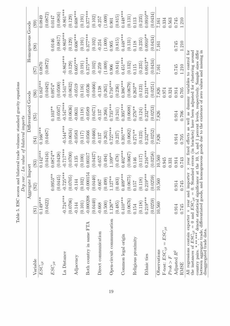
contracting and negotiation costs. Table 5 reports our results.

Let us first focus on country i′s aggregate imports from j (columns (S1) to

(S3)). Specification (S1) regresses i′s imports on the scores that i allots to j.

Specification (S2) instead inverts the direction of scoring and uses the ESC

scores that j awards to i. Column (S3) uses both directions in a single equation.

We include a dummy Dijt that takes the value of one if ESCijt > 0 and zero

otherwise (similarly for ESCjit).22 In all models, the ESC variables turn out

statistically highly significant and positive. Measures for the more conventional

cultural variables such as common language, legal system, religious proximity,

and ethnic ties continue to matter, their marginal effects being slightly smaller

than those reported in regressions without the ESC scores.

In section 2.2, we have argued that cultural proximity may have a low degree

of reciprocity. This conjecture implies that high scores awarded by country

i to j should foster i′s imports from j, but high scores awarded by j to i

need not increase i′s imports (but rather j′s). This hypothesis is confirmed

22 We do not report the estimates of Dijt since it is mostly insignificant. We owe thisdummy variable strategy to an anonymous referee. The bilateral trade variable isin fact not affected by the failure to rank songs below 1 to 10 so that our estimationstrategy is not plagued by non-random sampling.

18

Tab

le5.

ESC

scor

esan

dbi

late

ral

trad

evo

lum

es:

stan

dard

grav

ity

equa

tion

sD

ep.v

ar.:

Ln

valu

eof

bila

tera

lim

port

s

Agg

rega

teIm

por

tD

iffer

enti

ated

Goods

Hom

ogen

eous

Goods

Var

iable

(S1)

(S2)

(S3)

(S4)

(S5)

(S6)

(S7)

(S8)

(S9)

ESCijt

0.14

9***

0.14

2***

0.16

6***

0.16

3***

0.08

700.

0849

(0.0

422)

(0.0

416)

(0.0

487)

(0.0

482)

(0.0

872)

(0.0

872)

ESCjit

0.09

53**

0.08

74**

0.10

3**

0.09

74*

0.01

460.

0147

(0.0

445)

(0.0

438)

(0.0

507)

(0.0

500)

(0.0

817)

(0.0

816)

Ln

Dis

tance

-0.7

24**

*-0

.725

***

-0.7

17**

*-0

.544

***

-0.5

47**

*-0

.541

***

-0.8

62**

*-0

.863

***

-0.8

61**

*

(0.0

706)

(0.0

705)

(0.0

700)

(0.0

634)

(0.0

636)

(0.0

632)

(0.1

29)

(0.1

29)

(0.1

29)

Adja

cency

-0.1

44-0

.144

-0.1

35-0

.058

3-0

.063

1-0

.051

90.

605*

**0.

606*

**0.

608*

**

(0.1

01)

(0.1

02)

(0.1

00)

(0.1

17)

(0.1

18)

(0.1

16)

(0.1

91)

(0.1

91)

(0.1

91)

Bot

hco

untr

yin

sam

eF

TA

-0.0

0020

8-0

.000

154

0.00

317

-0.0

566

-0.0

589

-0.0

536

0.37

5***

0.37

7***

0.37

7***

(0.0

440)

(0.0

440)

(0.0

437)

(0.0

466)

(0.0

471)

(0.0

466)

(0.1

02)

(0.1

02)

(0.1

02)

Dir

ect

com

munic

atio

n-0

.668

-0.6

67-0

.657

-0.1

37-0

.137

-0.1

38-0

.259

-0.2

54-0

.257

(0.5

00)

(0.4

99)

(0.4

94)

(0.2

63)

(0.2

66)

(0.2

65)

(1.0

09)

(1.0

09)

(1.0

09)

Op

en-c

ircu

itco

mm

unic

atio

n1.

126*

*1.

127*

*1.

109*

*0.

727*

**0.

735*

**0.

716*

**0.

906

0.90

50.

901

(0.4

85)

(0.4

83)

(0.4

78)

(0.2

37)

(0.2

41)

(0.2

36)

(0.8

14)

(0.8

15)

(0.8

15)

Com

mon

lega

lor

igin

0.41

0***

0.40

9***

0.40

2***

0.39

1***

0.39

5***

0.38

6***

0.45

1***

0.44

8***

0.44

8***

(0.0

676)

(0.0

675)

(0.0

667)

(0.0

682)

(0.0

688)

(0.0

679)

(0.1

32)

(0.1

31)

(0.1

31)

Rel

igio

us

pro

xim

ity

0.15

40.

157

0.14

60.

271*

*0.

276*

*0.

263*

*0.

115

0.11

80.

113

(0.1

18)

(0.1

18)

(0.1

17)

(0.1

23)

(0.1

24)

(0.1

23)

(0.2

35)

(0.2

35)

(0.2

35)

Eth

nic

ties

0.21

9***

0.21

9***

0.21

6***

0.23

2***

0.23

2***

0.23

1***

0.09

13**

0.09

10**

0.09

10**

(0.0

259)

(0.0

259)

(0.0

258)

(0.0

252)

(0.0

253)

(0.0

251)

(0.0

434)

(0.0

434)

(0.0

434)

Obse

rvat

ions

10,5

6010

,560

10,5

607,

826

7,82

67,

826

7,16

17,

161

7,16

1

F-t

est:ESCijt

=ESCjit

0.94

50.

974

0.33

4

Prob>F

0.33

10.

324

0.56

3

Adju

sted

R2

0.91

40.

914

0.91

40.

914

0.91

40.

914

0.74

50.

745

0.74

5

RM

SE

0.74

50.

745

0.74

30.

705

0.70

60.

705

1.21

01.

210

1.21

0

All

regr

essi

ons

cont

ain

expo

rter×

year

and

impo

rter×

year

fixed

effec

tsas

wel

las

dum

my

vari

able

sto

cont

rol

for

the

inst

ance

sof

ES

Cijt

=0

and

ES

Cjit

=0.

Stan

dard

erro

rs(i

nbr

acke

ts)

have

been

adju

sted

for

clus

teri

ngar

ound

coun

try

pair

s.*,

**,*

**de

note

stat

isti

cal

sign

ifica

nce

atth

e10

,5,

and

1pe

rcen

tle

vels

,re

spec

tive

ly.

Sam

ple

size

sdi

ffer

betw

een

aggr

egat

etr

ade,

diffe

rent

iate

dgo

ods,

and

hom

ogen

eous

good

sdu

eto

the

exis

tenc

eof

zero

valu

esan

dm

issi

ngin

disa

ggre

gate

dtr

ade

data

.

19

in specification (S2). The coefficient on the ESCjit variable is positive, but

smaller and estimated with a lower degree of precision than the ESCijt variable

in (S1). The effect on aggregate imports of moving the ESC for the importing

country from 0 to 1 is 14.9% in specification (S1). The effect of the ESC scores

for the exporting country is 9.53% in specification (S2).

Specification (S3) uses both ESC variables simultaneously in the same regres-

sion. Estimated coefficients are strikingly close to those obtained separately

in columns (S1) and (S2). This fact can be interpreted as a lack of strong

correlation between ESCijt and ESCjit and therefore as a sign of low reci-

procity. Moreover, country i′s imports receive a stronger boost from higher

realizations of ESCijt than ESCjit. An F-test on the difference between the

two estimates of the ESC scores in specification (S3) does not allow rejecting

the conclusion that this difference is statistically zero. But the fact that both

variables enter signficantly and simultaneously argues the other way.

Columns (S4) to (S6) and (S7) to (S9) repeat this exercise for differentiated

and homogeneous goods, respectively. Results for the subaggregate of differen-

tiated goods are comparable to those for aggregate trade. Results for homoge-

neous goods, however, are different. Most strikingly, we find that ESC scores

matter for trade in differentiated goods regardless of the exact specification of

the model, while they are irrelevant for trade in homogeneous goods. Moving

the ESC for the importing country from 0 to 1 impacts trade in differentiated

goods by 16.6% in specification (S4). The effect of the ESC scores for the

exporting country is 10.3% in specification (S5).

The failure of ESC scores to show up significantly in the specifications explain-

ing trade in homogeneous goods is in contrast to the conventional measures of

cultural proximity, such as common legal origin and ethnic ties whose effects

on bilateral trade come out positive and statistically significant. Moreover,

the adjacency variable turn out significant for trade of homogeneous goods. 23

The literature suggests that informal trade costs, such as those represented by

23 FTA membership seems to matter for homogeneous goods, but is unimportantfor trade in differentiated goods. This is a surprising and interesting result thatmay be worth further investigation.

20

cultural distance should matter more for complex differentiated goods, which

are difficult to contract over. Middlemen selling homogeneous goods usually

do not reveal the country of production, so that the operation of a preference

channel would be hard to defend. Taking the extreme position that cultural

proximity is entirely irrelevant for homogeneous goods, the conventional in-

dicators must affect trade costs through a mechanism unrelated to cultural

proximity. Hence, this evidence supports the interpretation of ESC scores as

operating strictly through an influence on tastes.

Following Anderson and van Wincoop (2004), we can also interpret the ESC

coefficients in term of an accross-the-board tariff equivalent. In order to do

this we assume that the elasticity of substitution to 6 for aggregate trade, to

4 for differentiated goods, and to 12 for homogeneous goods. Thus, moving

ESCijt scores from 0 to 1 is equivalent to reducing tariff by 2.37 for aggre-

gate imports (0.142 × 100/6) and by 4.1 percentage points for differentiated

products (0.163× 100/4).

5 Extensions

In this section we present a number of critical extensions dealing with the

endogeneity of cultural proximity and the omitted variable problem. We also

present several robustness checks to assess our main results.

5.1 Controlling for endogeneity

There is a growing theoretical literature on the endogenous emergence and

evolution of cultural identities (see the recent surveys by Fernandez, 2007 and

Guiso et al., 2009). This literature identifies determinants that drive both

economic outcomes and cultural traits. In the context of the present paper,

positive shocks on bilateral trade volumes could lead to cultural convergence

so that two countries end up with a higher degree of cultural proximity than

before the shock. Regressing ESC scores on lagged bilateral trade (imports,

21

exports, or the sum thereof), and controlling for dyadic fixed effects, we do

not find any first-order evidence for endogeneity. This result is confirmed in

a number of models that differ with respect to their treatment of the non-

linearity of ESC scores (OLS, Tobit, and Poisson). But while this evidence is

suggestive, it is not a rigorous proof on the absence of endogeneity. It is still

possible that OLS estimates suffer from simultaneity bias. Dealing with the

simultaneity problem requires an instrumentation strategy.

Following Combes et al. (2005), we exploit the time structure of our data to

estimate the effect of an exogenous change in cultural proximity. It is reason-

able to assume that past ESC scores (e.g., dating from t− 5), are not causally

affected by current bilateral trade volumes (at time t). In other words, current

shocks in the gravity equation are uncorrelated to lagged ESC values. Then,

past ESC scores are valid instruments, provided that they predict current

scores sufficiently well.

Table 6 presents instrumental variable 2SLS regressions. 24 As usual, we com-

pare aggregate trade, trade in differentiated goods, and trade in homogeneous

goods and either use ESCijt and ESCjit separately (specifications (1), (2),

(4), (5), (7), (8)) or simultaneously (specifications (3), (6), and (9)). The

first-stage regressions typically have F-statistics well beyond the usual rule-

of-thumb value of 10. We also report the Durbin and Wu-Hausman statistics.

They do not allow to test exogeneity of the regressors per se, but whether the

coefficients of more-efficient OLS estimation differ significantly from the coef-

ficients of consistent but less efficient 2SLS estimation. Typically, we have to

reject exogeneity at high degrees of significance; specifications (S5) and (S8)

are notable exceptions. Hence, in general, instrumentation is required, and the

proposed instrumentation strategy is valid. 25

The IV results confirm a positive and significant effect of ESC scores on bilat-

eral trade. Typically, the regressions reveal that the country i′s imports are

24 Results based on GMM or limited information maximum likelihood methodsperform very similarly.

25 The first stage regressions signal that 5-year lags of scores are valid instruments.Shorter lag structures work as well, but to the extent that bilateral trade flows arepersistent, are less suited as instruments. Longer lags yield first stage regressionswith fairly low F statistics.

22

Tab

le6.

IVR

egre

ssio

ns(I

nstr

umen

tis

5th

tim

ela

gof

ESC

scor

e)D

ep.v

ar.:

Ln

valu

eof

bila

tera

ltr

ade

Agg

rega

teIm

por

tsD

iffer

enti

ated

Goods

Hom

ogen

eous

Goods

Var

iable

(S1)

(S2)

(S3)

(S4)

(S5)

(S6)

(S7)

(S8)

(S9)

ESCijt

1.75

7***

1.40

0**

1.06

4**

0.95

1*2.

707*

**2.

980*

**

(0.4

74)

(0.5

52)

(0.4

79)

(0.5

26)

(0.9

19)

(1.1

15)

ESCjit

1.54

7***

1.06

7*0.

677

0.41

8-0

.021

7-0

.943

(0.4

50)

(0.5

48)

(0.4

50)

(0.5

20)

(0.9

27)

(1.3

30)

Ln

Dis

tance

-0.4

92**

*-0

.504

***

-0.4

46**

*-0

.297

***

-0.3

17**

*-0

.281

***

-0.6

10**

*-0

.746

***

-0.6

52**

*

(0.0

402)

(0.0

386)

(0.0

419)

(0.0

364)

(0.0

345)

(0.0

383)

(0.0

740)

(0.0

726)

(0.0

913)

Adja

cency

0.03

390.

0208

0.07

420.

164*

**0.

138*

**0.

183*

**0.

654*

**0.

501*

**0.

599*

**

(0.0

541)

(0.0

517)

(0.0

548)

(0.0

557)

(0.0

527)

(0.0

573)

(0.1

11)

(0.1

06)

(0.1

33)

Bot

hco

untr

yin

sam

eF

TA

0.04

710.

0394

0.07

20**

0.02

640.

0065

70.

0420

0.55

5***

0.41

1***

0.52

0***

(0.0

316)

(0.0

303)

(0.0

321)

(0.0

358)

(0.0

338)

(0.0

376)

(0.0

738)

(0.0

663)

(0.0

855)

Dir

ect

com

munic

atio

n-0

.499

***

-0.5

04**

*-0

.495

***

-0.2

38-0

.227

-0.2

470.

107

0.15

60.

139

(0.1

37)

(0.1

32)

(0.1

36)

(0.1

53)

(0.1

45)

(0.1

52)

(0.3

61)

(0.2

99)

(0.3

82)

Op

en-c

ircu

itco

mm

unic

atio

n0.

979*

**0.

987*

**0.

957*

**0.

820*

**0.

835*

**0.

809*

**0.

616*

0.75

1***

0.63

3*

(0.1

25)

(0.1

20)

(0.1

24)

(0.1

38)

(0.1

32)

(0.1

37)

(0.3

19)

(0.2

62)

(0.3

36)

Com

mon

lega

lor

igin

0.31

1***

0.31

9***

0.28

3***

0.26

3***

0.28

7***

0.24

4***

0.33

0***

0.48

9***

0.37

3***

(0.0

358)

(0.0

345)

(0.0

365)

(0.0

424)

(0.0

400)

(0.0

446)

(0.0

844)

(0.0

790)

(0.1

01)

Rel

igio

us

pro

xim

ity

0.09

150.

104*

0.03

980.

356*

**0.

391*

**0.

332*

**0.

116

0.36

3***

0.16

7

(0.0

622)

(0.0

600)

(0.0

635)

(0.0

665)

(0.0

622)

(0.0

685)

(0.1

44)

(0.1

22)

(0.1

59)

Eth

nic

ties

0.17

2***

0.17

8***

0.16

2***

0.21

3***

0.21

5***

0.21

0***

0.05

96**

*0.

0707

***

0.06

48**

*

(0.0

119)

(0.0

111)

(0.0

121)

(0.0

101)

(0.0

0965

)(0

.010

2)(0

.021

4)(0

.018

4)(0

.023

4)

Obse

rvat

ions

5,89

05,

890

5,89

04,

457

4,45

74,

457

4,21

14,

211

4,21

1

RM

SE

0.70

80.

681

0.70

40.

604

0.57

40.

598

1.26

91.

046

1.33

6

adju

sted

R2

0.89

20.

900

0.89

30.

915

0.92

30.

917

0.65

50.

766

0.61

8

ESCijt

=ESCjit,χ

20.

120.

353.

36*

ESCijt

=0∩ESCjit

=0,χ

223

.75*

**6.

92**

7.85

**

Durb

in(s

core

)17

.479

***

14.0

48**

*28

.408

***

4.28

1**

1.67

5.34

0*13

.262

***

0.01

813

.072

***

Wu-H

ausm

anF

15.2

46**

*12

.246

***

12.4

07**

*3.

681*

1.43

52.

295

11.3

16**

*0.

015

5.57

4***

Fir

st-s

tage

F27

.599

***

28.3

15**

*19

.512

***

19.9

92**

*23

.838

***

15.5

70**

*

All

regr

essi

ons

cont

ain

expo

rter×

year

and

impo

rter×

year

fixed

effec

ts.

Stan

dard

erro

rs(i

nbr

acke

ts)

have

been

adju

sted

for

clus

teri

ngar

ound

coun

try

pair

s.*,

**,*

**de

note

stat

isti

cal

sign

ifica

nce

atth

e10

,5,

and

1pe

rcen

tle

vels

,re

spec

tive

ly.

Sam

ple

size

sdi

ffer

betw

een

aggr

egat

etr

ade,

diffe

rent

iate

dgo

ods,

and

hom

ogen

eous

good

sdu

eto

the

exis

tenc

eof

zero

valu

esan

dm

issi

ngin

disa

ggre

gate

dtr

ade

data

.

23

more strongly spurred by higher realizations of ESCijt than of ESCjit, which

confirms a finding presented in Table 5. However, as the χ2 tests on equality

of coefficients performed in columns (3), (6) and (9) show, we do not always

have strong statistical evidence for the differential impact of these two vari-

ables. Also note that the χ2 test on ESCijt = ESCijt = 0 typically fails, so

that cultural proximity of some type always matters in the proposed models.

The IV results imply that OLS biases the effect of ESC scores downwards. On

the one hand, one would expect that a positive shock on trade increases cul-

tural proximity. However, on the other hand, it is important to notice that the

IV-regressions not only remedy a potential endogeneity bias, they also help

to deal with measurement error, which biases OLS estimates towards zero.

While our analysis leaves little doubt on the meaningfulness of ESC scores as

measures of cultural proximity, it is also obvious that these scores are very

noisy proxies.

Guiso et al. (2009) and Combes et al. (2005) also discuss attempts to use IV

strategies in similar setups, where the level of bilateral economic activity is

regressed on various measures of bilateral trust or information. Both papers

find that OLS strongly underestimates the true causal effects, just as we find

in our 2SLS regressions. Both papers conclude that ‘reverse causality is not

a major problem’. This is a strong conclusion; however, we have found no

contradictory evidence.

5.2 Controlling for unobserved factors

The volume of trade between two countries and the degree of cultural proxim-

ity between them may both depend on bilateral factors that remain unobserved

by the econometrician. Often, these factors are related to initial conditions.

There are at least three examples of unobserved factors that may be relevant

in the context of this paper.

First, cross-border transactions require and condition social interactions be-

tween individuals, which may change their incentives to acquire certain skills

or invest in certain networks. For example, interactions with foreign trading

24

partners at some initial point in time might lead to mutual learning, which

may trigger convergence of cultural characteristics as certain norms or behav-

ioral standards are adopted. In turn, this generates more trade, potentially

through both the trade cost and the preference channel. Hence, current lev-

els of bilateral trade and cultural proximity positively depend on the initial

degree of cultural proximity. This, in turn, means that failing to control for

initial conditions distorts estimates upwards due to omitted variable bias.

A second problem, closely related to the first, is habit formation. The pref-

erence for a country’s specific varieties may be stronger if the representative

consumer in the partner country already heavily consumes those varieties.

Again, it is the unobserved initial bilateral trade volume that may have led to

the endogenous formation of consumption habits and, hence, bias estimates.

Third, the volume of trade between two countries and the degree of cultural

proximity between them may both depend on geographical factors. For exam-

ple, bilateral migration between two countries may affect cultural proximity

and trade alike. However, one set of determinants for migration is geographical

distance or adjacency – two factors that we can easily control for. The other

set of determinants has to do with income levels, and those depend on mul-

tilateral trade and not bilateral trade. In our regressions we also control for

aggregate trade, since we have included country × year fixed effects. However,

there may be remaining unobserved bilateral determinants of migration.

One way to deal with initial conditions is to use dyad-specific fixed effects. In

the presence of those effects, the influence of the ESC scores depends entirely

on their movement over time. The cross-sectional effects of the scores are

absorbed by the dyadic fixed effects. Baier and Bergstrand (2007) successfully

use this strategy in the gravity equation context. We estimate the following

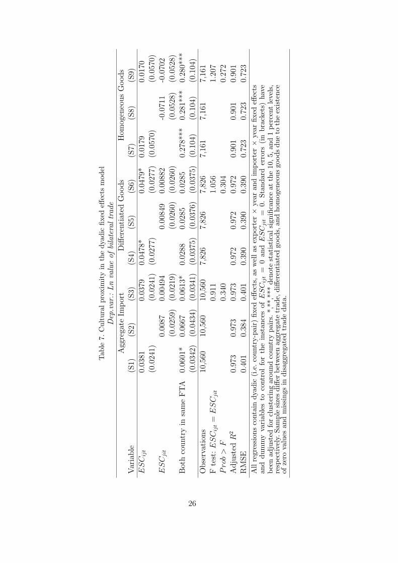
‘dyadic fixed effects equation’ (DFEE) model:

lnMijt = ηESCijt + ϕFTAijt + νit + νjt + νij +Dijt + εijt, (8)

where νij denotes the comprehensive set of country-pair specific fixed effects.

Compared to equation (7), the inclusion of νij makes all time-invariant bi-

25

Tab

le7.

Cul

tura

lpr

oxim

ity

inth

edy

adic

fixed

effec

tsm

odel

Dep

.var

.:L

nva

lue

ofbi

late

ral

trad

e

Agg

rega

teIm

por

tD

iffer

enti

ated

Goods

Hom

ogen

eous

Goods

Var

iable

(S1)

(S2)

(S3)

(S4)

(S5)

(S6)

(S7)

(S8)

(S9)

ESCijt

0.03

810.

0379

0.04

78*

0.04

79*

0.01

790.

0170

(0.0

241)

(0.0

241)

(0.0

277)

(0.0

277)

(0.0

570)

(0.0

570)

ESCjit

0.00

870.

0049

40.

0084

90.

0088

2-0

.071

1-0

.070

2

(0.0

259)

(0.0

219)

(0.0

260)

(0.0

260)

(0.0

528)

(0.0

528)

Bot

hco

untr

yin

sam

eF

TA

0.06

01*

0.06

670.

0613

*0.

0288

0.02

850.

0285

0.27

8***

0.28

1***

0.28

0***

(0.0

342)

(0.0

434)

(0.0

341)

(0.0

375)

(0.0

376)

(0.0

375)

(0.1

04)

(0.1

04)

(0.1

04)

Obse

rvat

ions

10,5

6010

,560

10,5

607,

826

7,82

67,

826

7,16

17,

161

7,16

1

Fte

st:ESCijt

=ESCjit

0.91

11.

056

1.20

7

Prob>F

0.34

00.

304

0.27

2

Adju

sted

R2

0.97

30.

973

0.97

30.

972

0.97

20.

972

0.90

10.

901

0.90

1

RM

SE

0.40

10.

384

0.40

10.

390

0.39

00.

390

0.72

30.

723

0.72

3

All

regr

essi

ons

cont

ain

dyad

ic(i

.e.c

ount

ry-p

air)

fixed

effec

ts,a

sw

ella

sex

port

er×

year

and

impo

rter×

year

fixed

effec

tsan

ddu

mm

yva

riab

les

toco

ntro

lfo

rth

ein

stan

ces

ofE

SCijt

=0

and

ES

Cjit

=0.

Stan

dard

erro

rs(i

nbr

acke

ts)

have

been

adju

sted

for

clus

teri

ngar

ound

coun

try

pair

s.*,

**,*

**de

note

stat

isti

cals

igni

fican

ceat

the

10,5

,and

1pe

rcen

tle

vels

,re

spec

tive

ly.S

ampl

esi

zes

diffe

rbe

twee

nag

greg

ate

trad

e,di

ffere

ntia

ted

good

s,an

dho

mog

eneo

usgo

ods

due

toth

eex

iste

nce

ofze

rova

lues

and

mis

sing

sin

disa

ggre

gate

dtr

ade

data

.

26

lateral determinants redundant. In particular, variables such as common lan-

guage, common legal origin, etc., of trade flows drop out.

Table 7 reports the results from running regression (8) on our data set. As al-

ways, we differentiate between aggregate trade, trade in differentiated goods,

and trade in homogeneous goods, but also between ESC scores for the import-

ing and the exporting country. Since identification of the coefficients draws

only on time variance, it becomes more difficult to find significant results.

Yet with dyadic and country × year fixed effects included in the regression,

we still find that ESC scores retain a positive and statistically significant in-

fluence on bilateral trade but only the in the case of trade in differentiated

goods and only for country i’s imports from j; see columns (S4) and (S5). The

significant influence on bilateral trade in differentiated goods – now smaller

than before – also holds up when both ESC measures are used simultaneously

in the regression; see column (S6). Moving ESCijt scores from 0 to 1 would

be equivalent to reducing an ad valorem tariff by 1.20 percentage points in

specification (S6). 26

5.3 Additional robustness checks

We have carried out two additional robustness checks, which can be consulted

in the web appendix to this paper. One has to do with the switch from jury-

based voting to televoting which occurred in 1998. Since our data extends

from 1975 to 2003, one may wonder whether our results are driven by this

switch in the rules of the contest. Table 1 shows regression results for the

period 1975-1998, thereby drawing only on scores established by juries rather

than by televoting. Our main results remain fully intact qualitatively. The total

pro-trade effect of cultural proximity turns out slightly lower. The effect of the

ESC scores for the exporting country turns out insignificant. For homogeneous

goods, there is no robust effect of cultural proximity on trade, as in the main

body of the paper.

26 0.0479×100/4.

27

One may also question to what extent our results are driven by changes in

bilateral migration stocks. The country that sent most immigrants to Europe

during the period under investigation has been Turkey. Most of Turkish em-

igrants went to Germany. The bilateral stocks of immigrants at the start of

our sample changed little since then due to restrictive immigration policies

(Boeri and Brucker, 2005). Another test we provide then is to exclude is to

exclude the dyad-specific fixed effects for Turkey as the sending country and

to leave out the German-Turkish pair from our regressions in Table 2. The

results resemble the earlier ones with all of the dyadic-specific effects.

6 Conclusions

There are many anecdotal hints that cultural proximity is a major determinant

of bilateral trade volumes. However, empirical quantification and testing are

difficult due to the elusiveness of the concept and lack of observability. The

existing literature tries to account for cultural proximity by including vari-

ables such as common language, common legal origins, religious proximity, or

ethnic ties. These indicators are certainly connected to cultural affinity be-

tween nations; they do, however, also capture other things related to the cost

of contracting and negotiation that do not have anything to do with culture.

We show that there is more to cultural proximity than what the conventional

variables allow.

In this paper we draw on bilateral score data from the Eurovision Song Contest

(ESC), a very popular pan-European television show, to construct a measure

of cultural proximity which varies over time and within country pairs, and that

correlates strongly with conventional indicators. Within the framework of a

theory-grounded gravity model, we show that our measure positively affects

trade in differentiated goods, even after controlling for the conventional mea-

sures used in the literature. Further, ESC scores do not add any explanatory

power to gravity equations for goods that are traded on organized exchanges

while the conventional indicators continue to matter. This is perfectly sensible.

Since cultural proximity should not matter when direct contacts between sell-

28

ers and buyers are not required. This finding suggests that ESC scores indeed

reflect cultural proximity alone while the standard variables are also related

to the costs of negotiating and contracting.

These results are surprisingly robust. We are able to reject that they are

driven by simultaneity bias. They also survive the inclusion of country-pair

specific fixed effects so that our baseline findings are not due to the omission of

unobserved factors neither. Hence, our study highlights the overall importance

of cultural proximity as well as the role of its time-varying and asymmetric

nature for the determination of bilateral trade volumes.

29

1 Summary Statistics and Data Sources

Our dataset and the web appendix can be downloaded at http://team.univ-

paris1.fr/teamperso/toubal/papers/CP/CP.html.

Aggregate imports. Aggregate bilateral import flows (measured c.i.f.)

are from the IMF’s Direction of Trade Statistics (DoTS) CDROM (July 2006

edition) for the period 1975-2003.

Trade in differentiated and homogeneous goods. The data has been

constructed by aggregating SITC4 rev. 2 trade data (c.i.f.) prepared by Feen-

stra et al. (2005) according to Rauch’s (1999) ‘conservative’ classification of 4

digit SITC goods for the period 1975-2000.

Raw ESC scores. Data are from http://www.kolumbus.fi/jarpen/.

An alternative website is http://nul-points.net/.

Adjusted ESC scores. Adjusted ESC scores are the residual of a regres-

sion of raw ESC scores on a set of song dummies.

Conventional measures of cultural proximity. We are very thankful

to Jacques Melitz for sharing his data on languages. The variables have been

computed as in Melitz (2008). We add Russian to his major direct communi-

cation languages since we have bilateral trade data for Russia. The measure

‘common legal origin’ is taken from La Porta et al. (1999) and distinguishes

between a Latin, a Scandinavian, a British, and a Germanic system.

Following Alesina et al. (2000), ‘religious proximity’ is constructed as follows:

Using mid-1990ies Census data 27 , we compute the shares sri of adherents

to religion r ( Catholics, Protestants, orthodox Christians, Muslims, Jews,

atheists, and non-religious persons) in total population of country i. Then,

we compute a bilateral index ρij =∑r srisrj, with ρij ∈ [0, 1] . This measure

reaches a maximum value of 0.85 for the dyad Poland-Malta, and is minimum,

0.001, for the pair Poland-Turkey.

27 The data are freely available on www.worldchristiandatabase.org and coincideclosely with entries in the CIA fact book and other sources.

30

Tab

le1.

Sum

mar

ySt

atis

tics

Aggre

gate

Imp

ort

sD

iffere

nti

ate

dgoods

Hom

ogeneous

goods

(N=

10,5

60)

(N=

7,82

6)(N

=7,

161)

Var

iable

Mea

nStd

.D

ev.

Mea

nStd

.D

ev.

Mea

nStd

.D

ev.

Ln

trad

e19

.096

2.54

018

.490

2.40

916

.609

2.39

8

ESCijt

0.26

70.

340

0.27

00.

341

0.27

60.

343

ESCjit

0.26

70.

340

0.27

10.

341

0.27

40.

342

Ln

dis

tance

7.30

60.

627

7.32

10.

616

7.29

30.

624

Adja

cency

0.09

10.

287

0.08

70.

282

0.09

50.

293

Bot

hco

untr

yin

sam

eF

TA

0.30

80.

462

0.32

80.

469

0.34

90.

477

Dir

ect

com

munic

atio

n0.

026

0.14

10.

025

0.13

60.

026

0.13

9

Op

en-c

ircu

itco

mm

unic

atio

n0.

024

0.15

30.

020

0.14

00.

022

0.14

6

Com

mon

lega

lor

igin

0.18

30.

387

0.19

50.

396

0.20

50.

403

Rel

igio

us

pro

xim

ity

0.21

00.

248

0.22

10.

258

0.22

30.

255

Eth

nic

ties

7.74

02.

835

7.73

12.

555

8.00

92.

395

31

As a measure of ethnic ties, we use the stock of foreign born individuals

by country of birth, provided by the OECD and discussed in Dumont and

Lemaitre (2005). Our regressions include the natural logarithm of that stock.

Geographical data. Geographical distance and adjacency are from the

CEPII in Paris. 28

Free trade agreements. Data is from Baier and Bergstrand (2006) and

updated to account for the pre-EU membership Europe agreements signed by

East European countries with the EU (WTO website).

28 The CEPII data can be downloaded fromwww.cepii.fr/anglaisgraph/bdd/distances.htm.

32

References

• Alesina, A., Dollar, D., 2000. Who Gives Foreign Aid to Whom and Why.

Journal of Economic Growth 5, 33-64.

• Algan, Y., and Cahuc, P., 2007. Social Attitudes and Macroeconomic Perfor-

mance: An Epidemiological Approach. Mimeo: Paris School of Economics.

• Anderson, J.E., Van Wincoop, E., 2003, Gravity with Gravitas: A Solution

to the Border Puzzle. American Economic Review 03(1): 170-192.

• Anderson, J.E., Van Wincoop, E., 2004, Trade Costs. Journal of Economic

Literature 32(3): 691-751.

• Baier, S.L., Bergstrand, J.H., 2007, Do Free Trade Agreements Actually

Increase Members’ International Trade? Journal of International Economics

71(1): 72-95.

• Baltagi, B.H., Egger, P., Pfaffermayr, M., 2003, A Generalized Design For

Bilateral Trade Flow Models. Economics Letters 80: 391-397.

• Blum, B., and Goldfarb A., 2006. Does the Internet Defy the Law of Gravity.

Journal of International Economics 70(2): 384-405.

• Boeri, T., and Brucker, H., 2005. Why are Europeans so tough on migrants?

Economic Policy 44: 629–703.

• Boisso, D., Ferrantino, M., 1997, Economic Distance, Cultural Distance, and

Openness in International Trade: Empirical Puzzles. Journal of Economic

Integration 12(4): 456-484.

• Boeri, T., and Brucker, H., 2005. Why Europeans Are So Tough on Mi-

grants. Economic Policy, October 2005 : 629-703.

• Clerides, S., Stengos, T., 2006. Love thy Neighbor, Love thy Kin: Voting

Biases in the Eurovision Song Contest. Mimeo: University of Cyprus.

• Combes, P-P., M. Lafourcade and T. Mayer, 2005. The Trade Creating

Effects of Business and Social Networks: Evidence from France, Journal of

International Economics 66:1-29.

• Disdier, A.C., Mayer, T., 2007. Je T’aime, Moi Non Plus. Bilateral Opinions

and International Trade. European Journal of Political Economy 23: 1140-

1159.

• Disdier, A.C., Tai, S.H.T., Fontagne, L., and Mayer, T., 2007. Bilateral

33

Trade of Cultural Goods. Mimeo: University of Paris I.

• Dumont, J.-C. and Lemaitre, G., 2005, Counting immigrants and expatri-

ates: A new perspective. OECD Social, Employment and MigrationWorking

Paper 25.

• Feenstra, R. C., 2004. Advanced International Trade. Theory and Evidence.

Princeton: Princeton University Press.

• Feenstra, R. C., Lipsey, R.E., Deng, H., Ma, A.C., and Mo, H., 2005. World

Trade Flows: 1962-2000. NBER Working Paper 11040.

• Felbermayr, G., Toubal, F., 2006. Cultural Proximity and Trade. Tubinger

Diskussionsbeitrag Nr. 305.

• Fenn, D., O. Suleman, Efstathiou, J., Johnson, N.F., 2006. How does Eu-

rope Make Its Mind Up? Connections, cliques, and compatibility between

countries in the Eurovision Song Contest. Physica A 360(2): 576-598.

• Fernandez, R., 2007. Culture and Economics. New Palgrave Dictionary of

Economics, 2nd ed., edited by Durlauf, S.N., and Blume, L.E., Palgrave

McMillan, New York.

• Frankel,, J.A., 1997. Regional Trading Blocs in the World Economic System.

Institute for International Economics.

• Gatherer, D., 2006. Comparison of Eurovision Song Contest Simulation with

Actual Results Reveals Shifting Patterns of Collusive Voting Alliances. Jour-

nal of Artificial Societies and Social Simulation 9(2);

http://jasss.soc.surrey.ac.uk/9/2/1.html.

• Ginsburgh, V., Noury, A., 2008. The Eurovision Song Contest. Is voting

political or cultural, European Journal of Political Economy 24(1): 41-52..

• Ginsburgh, V., 2005. Languages, Genes, and Cultures. Journal of Cultural

Economics 29(1), 1-17.

• Giuliano, P., Spilimbergo, A., and Tonon, G., 2006. Genetic, Cultural and

Geographical Distances. IZA Working Paper 2229.

• Guiso, L., Sapienza, P., and Zingales, L., 2009. Cultural Biases in Economic

Exchange? The Quarterly Journal of Economics, forthcoming.

• Guiso, L., Sapienza, P., and Zingales, L., 2006. Does Culture Affect Eco-

nomic Outcomes? Journal of Economic Perspectives 20(2): 23-48.

• Greene, W.H., 2008, Econometric Analysis, Sixth Edition, Pearson, New

Jersey.

34

• Haan, M.A., Djikstra, G.S., Dijkstra, P.T., 2005. Expert Judgment versus

Public Opinion. Evidence from the Eurovision Song Contest. Journal of

Cultural Economics 29(1): 59-78.

• Huang, R.R., 2007. Distance and Trade: Disentangling Unfamiliarity Effects

and Transportation Cost Effects. European Economic Review 51: 161-181.

• La Porta, R., Shleifer, A., Vishny, R.W., Lopez Da Silanes, F., 1998. Law

and Finance. Journal of Political Economy 106(6).

• Melitz, J., 2008, Language and Foreign Trade, European Economic Review

52(4): 667-699.

• Rauch, J.E., 1999. Networks Versus Markets in International Trade. Journal

of International Economics 48(1): 7-35.

• Rauch, J.E., Trindade, V., 2002. Ethnic Chinese Networks in International

Trade. Review of Economics and Statistics 84(1): 116-130

• Rose, A.K., 2004. Do We Really Know that the WTO raises trade? American

Economic Review 94(1): 98-114.

• Spierdijek, L. and Vellekoop, M., 2008. The structure of bias in peer voting

systems: lessons from the Eurovision Song Contest. Empirical Economics:

DOI 10.1007/s00181-008-0202-5.

• Spolaore, E., and Wacziarg, R., 2009. The Diffusion of Development. Quar-

terly Journal of Economics, forthcoming.

• Straubhaar, J., 2002. (Re)asserting national television and national identity

against the global, regional and local levels of world television. In J. M. Chan

and B. T. McIntyre (eds.): In search of boundaries. Communication, nation-

States and cultural identities. Westport, Connecticut: Ablex Publishing.

• Tabellini, G., 2008. Institutions and Culture. Journal of the European Eco-

nomic Association 6(2-3): 255-294.

• Yair G. 1995. ‘Unite Unite Europe’ The political and cultural structures of

Europe as reflected in the Eurovision Song Contest. Social Networks 17(2):

147-161.

2 Web Appendix: Not to be Published

This Appendix provides additional information and tables to Cultural Prox-

35

imity and International Trade. Please also refer to Felbermayr and Toubal,

Tubinger Diskussionsbeitrag 305 at

http://team.univ-paris1.fr/teamperso/toubal/papers/CP/dpversion.pdf.

2.1 Time behavior of multilateral ESC scores

0.2

.4.6

.80

.2.4

.6.8

0.2

.4.6

.80

.2.4

.6.8

1980 1990 2000 1980 1990 2000 1980 1990 2000 1980 1990 2000 1980 1990 2000

AUT BEL CHE CYP DNK

ESP FIN FRA GBR GER

GRC IRL ISL ISR ITA

NLD NOR PRT SWE TUR

(mean) pop2 predicted pop2

Rev

eale

d po

pula

rity

Year

Graphs by graded countryFig. 1. Time profiles of multilateral scores obtained by countries.

36

Table 1

Taking into account the change in ESC’s rules

Televoting versus jury decision

Variables Aggregate Differentiated Homogeneous

Import Goods Goods

ESCijt 0.116** 0.120** 0.134

(0.046) (0.051) (0.093)

ESCjit 0.0507 0.0617 -0.0319

(0.048) (0.052) (0.087)

Ln Distance -0.599*** -0.479*** -0.855***

(0.073) (0.064) (0.13)

Adjacency -0.0706 -0.0279 0.637***

(0.10) (0.12) (0.20)

Both country in same FTA 0.0170 -0.0252 0.378***

(0.044) (0.047) (0.11)

Direct communication -0.621 -0.104 -0.263

(0.55) (0.27) (1.06)

Open-circuit communication 1.051** 0.724*** 0.963

(0.51) (0.24) (0.86)

Common legal origin 0.399*** 0.393*** 0.437***

(0.074) (0.072) (0.14)

Religious proximity 0.188 0.247** 0.0632

(0.13) (0.13) (0.25)

Ethnic ties 0.227*** 0.241*** 0.0826*

(0.029) (0.027) (0.049)

Observations 7,698 6,499 6,021

Adusted R2 0.920 0.917 0.744

RMSE 0.690 0.681 1.207

All regressions contain dyadic (i.e. country-pair) fixed effects, as well as

exporter × year and importer × year fixed effects and dummy variables

to control for the instances of ESCijt = 0 and ESCjit = 0. Standard

errors (in brackets) have been adjusted for clustering around country

pairs. *,**,*** denote statistical significance at the 10, 5, and 1 percent

levels, respectively. Sample sizes differ between aggregate trade, differen-

tiated goods, and homogeneous goods due to the existence of zero values

and missings in disaggregated trade data.

37

Table 2

Migration and ESC scores

Without the German-Turkish pair

Variables Aggregate Differentiated Homogeneous

Import Goods Goods

ESCijt 0.140*** 0.148*** 0.0885

(0.043) (0.049) (0.085)

ESCjit 0.0551 0.0904* 0.00811

(0.047) (0.052) (0.084)

Ln Distance -0.780*** -0.584*** -0.872***

(0.068) (0.064) (0.14)

Adjacency -0.109 0.0217 0.720***

(0.10) (0.12) (0.20)

Both country in same FTA 0.00115 -0.0392 0.379***

(0.045) (0.045) (0.11)

Direct communication -0.503 -0.112 -0.384

(0.46) (0.28) (0.99)

Open-circuit communication 1.093** 0.665*** 0.903

(0.46) (0.25) (0.80)

Common legal origin 0.368*** 0.384*** 0.331**

(0.065) (0.068) (0.14)

Religious proximity 0.114 0.275** 0.118

(0.12) (0.12) (0.24)

Ethnic ties 0.228*** 0.219*** 0.107**

(0.025) (0.026) (0.045)

Observations 9,610 7,286 6,651

Adusted R2 0.917 0.913 0.748

RMSE 0.723 0.699 1.204

All regressions contain dyadic (i.e. country-pair) fixed effects, as well as

exporter × year and importer × year fixed effects and dummy variables

to control for the instances of ESCijt = 0 and ESCjit = 0. Standard

errors (in brackets) have been adjusted for clustering around country

pairs. *,**,*** denote statistical significance at the 10, 5, and 1 percent

levels, respectively. Sample sizes differ between aggregate trade, differen-

tiated goods, and homogeneous goods due to the existence of zero values

and missings in disaggregated trade data.

38