G89.2247 Lecture 6 1

G89.2247SEM Lecture 6

• An Example

• Measures of Fit

• Complex nonrecursive models

• How can we tell if a model is identified?

• Direct and Indirect Effects

• Testing Indirect Effects

G89.2247 Lecture 6 2

An Example from JPSP: Effects of Resource Loss /Gain

JPSP September 1999 Vol. 77, No. 3, 620-629Resource Loss, Resource Gain, and Depressive Symptoms A 10-Year Model

Charles J. Holahan, Rudolf H. Moos, Carole K. Holahan, Ruth C. Cronkite

This study examined a broadened conceptualization of the stress and coping process that incorporated a more dynamic approach to understanding the role of psychosocial resources in 326 adults studied over a 10-year period. Resource loss across 10 years was significantly associated with an increase in depressive symptoms, whereas resource gain across 10 years was significantly associated with a decrease in depressive symptoms. In addition, change in the preponderance of negative over positive events across 10 years was inversely associated with change in resources during the period. Finally, in an integrative structural equation model, the association between change in life events and depressive symptoms at follow-up was completely mediated through resource change.

G89.2247 Lecture 6 3

The Model

G89.2247 Lecture 6 4

The Description of Fit

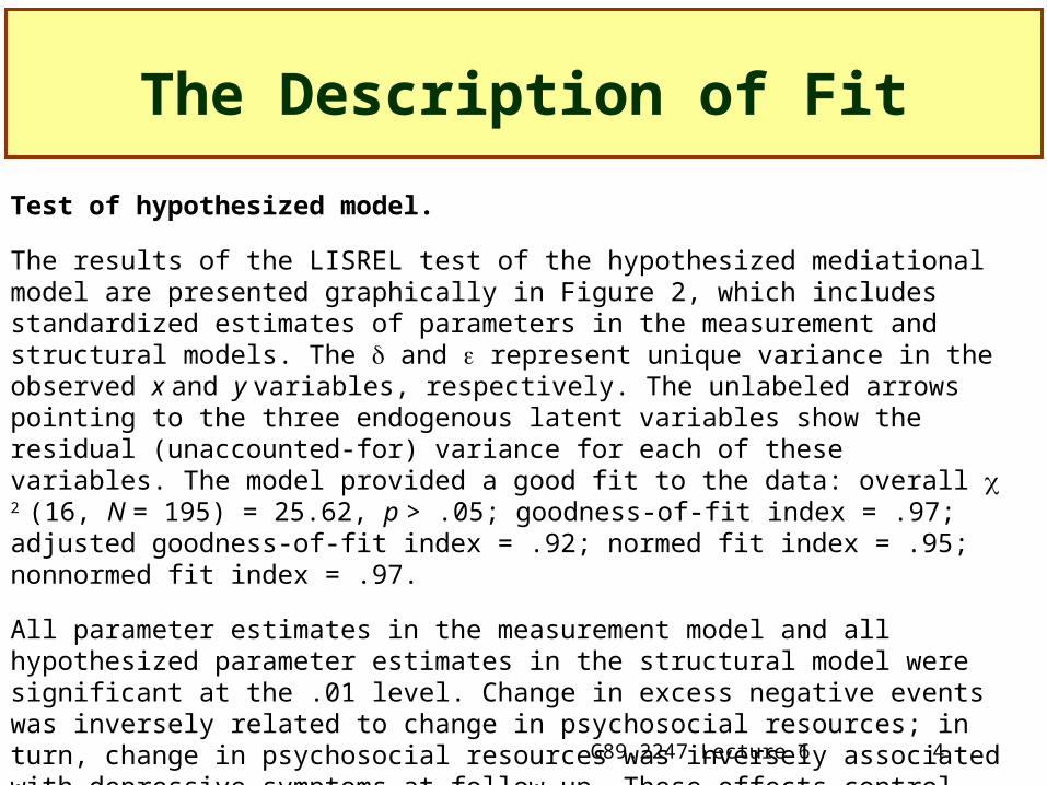
Test of hypothesized model.

The results of the LISREL test of the hypothesized mediational model are presented graphically in Figure 2, which includes standardized estimates of parameters in the measurement and structural models. The and represent unique variance in the observed x and y variables, respectively. The unlabeled arrows pointing to the three endogenous latent variables show the residual (unaccounted-for) variance for each of these variables. The model provided a good fit to the data: overall 2 (16, N = 195) = 25.62, p > .05; goodness-of-fit index = .97; adjusted goodness-of-fit index = .92; normed fit index = .95; nonnormed fit index = .97.

All parameter estimates in the measurement model and all hypothesized parameter estimates in the structural model were significant at the .01 level. Change in excess negative events was inversely related to change in psychosocial resources; in turn, change in psychosocial resources was inversely associated with depressive symptoms at follow-up. These effects control for the influence of initial depressive symptoms on all three endogenous variables. Thus, as we predicted, an increase in excess negative events showed an indirect relationship to an increase in depressive symptoms at follow-up, mediated by a decline in psychosocial resources. Initial depressive symptoms were not significantly related to changes in either events or resources.

G89.2247 Lecture 6 5

A Fit Measure Worth Considering:RMSEA

Root Mean Square Error of Approximation

where F is the minimized fitting function• Look for values less than .05

In example

dfndfLR

RMSEA)1(

056.016*194

)1662.25(

G89.2247 Lecture 6 6

Error of Approximation vs. Errors of Estimation

• Browne, M. W. and Cudeck, R. (1993) Alternative ways of assessing model fit. In Bollen, K.A. & Long, J.S. (eds) Testing structural equation models. Newbury Park, CA: Sage.

• When measurement models are considered along with structural models, almost all SEM models are misspecified to some extentWe should ask about that extentWe should distinguish between how close the model

approximates the true covariance structure and how fuzzy is our estimate of the model.

They find support for RMSEA as an index

G89.2247 Lecture 6 7

Revisiting the Holahan et al Structural Model

X1Y2

Y1

Y3

3

2

1

1

3

2

1

3

2

1

3

1

3

2

1

00

00

000

X

Y

Y

Y

b

b

Y

Y

Y

33

22

11

00

00

00

)(

Var

G89.2247 Lecture 6 8

Thinking about Correlated Residuals

• Holahan assume that the residuals are uncorrelated ( is diagonal) If there are response biases or other unmeasured

variables at work the residuals would be correlated.With uncorrelated residuals the model is recursive

• Easily shown to be identified

With completely correlated residuals, the model would not be identified.

G89.2247 Lecture 6 9

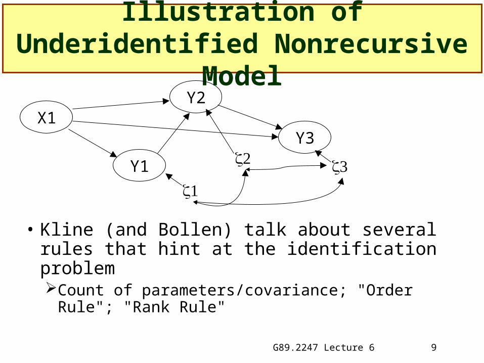
Illustration of Underidentified Nonrecursive Model

• Kline (and Bollen) talk about several rules that hint at the identification problemCount of parameters/covariance; "Order Rule";

"Rank Rule"

X1Y2

Y1

Y3

G89.2247 Lecture 6 10

Count of Parameters and Variance/Covariance Elements

• With 1+3=4 variables there are 4*3/2=6 covariances and 4 variances

• The model has five structural paths, three correlation paths, four variance estimatesThere are two too many parametersThese calculations do not tell us which parameters

need to be constrained

• The Counting rule is necessary but not sufficient to guarantee identification

G89.2247 Lecture 6 11

The Order Condition

• When one is interested in models with correlated residuals ( nondiagonal)

• Suppose we have p endogenous (Y) variables• For each endogenous variable

The number of excluded potential explanatory must be be greater or equal to (p-1)

We count both exogenous and endogenous explanatory variables

• This condition alerts us to equations that need to have more excluded explanatory variables.

G89.2247 Lecture 6 12

The Order Condition (Bollen’s Matrix Version)

• Suppose there are p endogenous variables and q exogenous variables

• is the pxp matrix of paths linking endogenous variables

• is the pxq matrix of paths linking endogenous variables to exogenous variables

• [ is a px(p+q) matrix summarizing all the possible explanatory paths

• C = [( is a px(p+q) matrix that is useful in counting for the order conditionEach row of C should have ≥(p-1) zeros

G89.2247 Lecture 6 13

Example of Order Condition

• Row 1 has two zeros, but rows two and three only have one zero each.

• The order condition is a necessary but not sufficient condition for identification.

33

21

1

00

00

000

b

b

33

21

1

10

01

001

b

bC

G89.2247 Lecture 6 14

Another Identification Check:The Rank Condition

• Consider the C= [(. For example

• Form three new smaller matrices, indexed by rowRetain columns that have zero’s in index row. E.g.

See if Rank(Ci)=(p-1). This holds for C1 but not C2,C3

33

21

1

10

01

001

b

bC

0

1

,

1

0

0

,

1

01

00

132

3

1 bCC

b

C

G89.2247 Lecture 6 15

SPSS can be used to help check Rank

COMMENT this illustrates some SPSS matrix manipulations.

MATRIX.

COMPUTE A={1, 1, 1;

2, 4, 8;

3, 9, 27}.

PRINT A.

COMPUTE B={1, 2, 3;

2, 3, 4;

3, 4, 5}.

PRINT B.

COMPUTE RANKA=RANK(A).

PRINT RANKA.

COMPUTE RANKB=RANK(B).

PRINT RANKB.

COMPUTE INVA=INV(A).

PRINT INVA.

COMPUTE D=INVA*B.

PRINT D.

COMPUTE RANKD=RANK(D).

PRINT RANKD.

COMPUTE E=A*D.

PRINT E.

END MATRIX.

G89.2247 Lecture 6 16

Checking an alternative just-identified model for Holahan

3

2

1

1

1

3

2

1

3

1

3

2

1

0

0

00

00

000

X

Y

Y

Y

b

b

Y

Y

Y

333231

2221

11

0

00

)(

Var

X1Y2

Y1

Y3

G89.2247 Lecture 6 17

Problems can still arise

• Inferences about correlated residuals come from relation of X to Y’sBut X1 and Y1 are barely relatedSee Handout

COVARIANCE MATRIX TO BE ANALYZED: 4 VARIABLES (SELECTED FROM 4 VARIABLES) BASED ON 326 CASES. V1 V2 V3 V4 V 1 V 2 V 3 V 4 V1 V 1 0.970 V2 V 2 0.049 1.012 V3 V 3 -0.088 -0.348 1.052 V4 V 4 0.575 0.276 -0.692 1.175

G89.2247 Lecture 6 18

Model as graphed can be shown to be identified with simulation

/TITLE Checking identification of JUST IDENTIFIED ALTERNATIVE TO Holahan model /SIMULATION POP=MOD; SEED=1209498; DATA='sm3'; SAVE=SEPARATE; REPLICATIONS=1; /SPECIFICATIONS VARIABLES= 4; CASES= 1000; METHODS=ML; MATRIX=RAW; /EQUATIONS V2 = + .7*V1 + E2; V3 = -.4*V2 + E3; V4 = -.6 *V3 + E4; /VARIANCES V1 = 1*; E2 = 1*; E3 = 1*; E4 = 1*; /COVARIANCES E3, E2 = 0*; E4, E2 = 0*; E4, E3 = 0*; /END

• This simulation makes V1 =>V2 connection strong• See handout

G89.2247 Lecture 6 19

Indirect Effects in Path Models

• Indirect effects of one variable on another are the effects that go through mediators.

• For recursive models we calculate indirect effects by forming products of mediating effects.

X1Y2

Y1

Y3

G89.2247 Lecture 6 20

Indirect Effects in Nonrecursive Models

• In nonrecursive models there is infinite regress

• The indirect effect can be estimated if the system is in equilibriumBollen shows that this is true if Bk →0 as k →This happens when absolute value of largest

eigenvalue of B is <1

Y2

Y1Y3

G89.2247 Lecture 6 21

Nonrecursive Equilibrium Models

ExogenousVariables

EndogenousVariables

Direct Effects

Indirect Effects

Total Effects

G89.2247 Lecture 6 22

Testing Indirect Effects

• LISREL, EQS, AMOS all compute large sample standard errors for indirect effects

• Baron and Kenny recommend using this standard error to test the indirect test using usual normal theory. Call the estimate IReject H0: indirect effect=0 if |[I/se(I)]|>1.96

However, test assumes that the estimate is normally distributed

Often the sampling distribution is skewed.

^^ ^

G89.2247 Lecture 6 23

A Bootstrap Confidence Interval for Indirect Effect

• Amos provides a convenient method for estimating sampling variability of the estimates of indirect effects.

• The use of the bootstrap is described in Shrout & Bolger (2002) Psychological Methods

• In the example, the indirect effect of Y1(V2) on Y3(V4) is .208 (.035) according to EQS.