G. Hager, G. Wellein Regionales Rechenzentrum...
37
High Performance High Performance Computing Computing Sequential Sequential code code optimization optimization by by example example G. Hager G. Hager , G. , G. Wellein Wellein Regionales Rechenzentrum Erlangen Regionales Rechenzentrum Erlangen W. u. E. W. u. E. Heraeus Heraeus Summerschool Summerschool on on Computational Computational Many Many Particle Particle Physics Physics Sep 18 Sep 18 - - 29, Greifswald, Germany 29, Greifswald, Germany
Transcript of G. Hager, G. Wellein Regionales Rechenzentrum...
High Performance High Performance ComputingComputingSequentialSequential codecode optimizationoptimization byby exampleexample
G. HagerG. Hager, G. , G. WelleinWelleinRegionales Rechenzentrum ErlangenRegionales Rechenzentrum Erlangen
W. u. E. W. u. E. HeraeusHeraeus SummerschoolSummerschoolon on ComputationalComputational ManyMany ParticleParticle PhysicsPhysicsSep 18Sep 18--29, Greifswald, Germany29, Greifswald, Germany

22.09.06 [email protected] 2Serial Optimization
A warning
“Premature optimization is the root of all evil.”Donald E. Knuth

22.09.06 [email protected] 3Serial Optimization
Outline
Warm-up example: Monte Carlo spin simulation „Common sense“ optimizations
Strength reduction by tabulationReducing the memory footprint
General remarks on algorithms and data accessExample: Matrix transpose
Data access analysisCache thrashingOptimization by padding and blocking
Example: Sparse matrix-vector multiplicationSparse matrix formats: CRS and JDSOptimizing data access for sparse MVMStrengths and weaknesses of the two formats
„„Common Common sensesense“ “ optimizationsoptimizations::A Monte Carlo A Monte Carlo spinspin codecode

22.09.06 [email protected] 5Serial Optimization
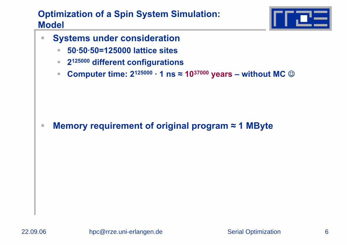
Optimization of a Spin System Simulation:Model
3-D cubic latticeOne variable („spin“) per gridpoint with values
+1 or -1
Next-neighbour interactiontermsCode chooses spinsrandomly and flips them as required by MC algorithm
22.09.06 [email protected] 6Serial Optimization
Systems under consideration50·50·50=125000 lattice sites2125000 different configurationsComputer time: 2125000 · 1 ns ≈ 1037000 years – without MC ☺
Memory requirement of original program ≈ 1 MByte
Optimization of a Spin System Simulation:Model
22.09.06 [email protected] 7Serial Optimization
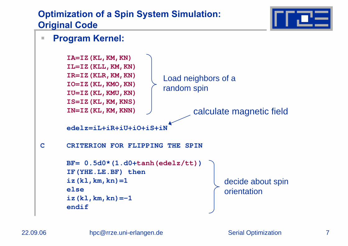
Optimization of a Spin System Simulation:Original Code
Program Kernel:
IA=IZ(KL,KM,KN) IL=IZ(KLL,KM,KN) IR=IZ(KLR,KM,KN) IO=IZ(KL,KMO,KN) IU=IZ(KL,KMU,KN) IS=IZ(KL,KM,KNS)IN=IZ(KL,KM,KNN)
edelz=iL+iR+iU+iO+iS+iN
C CRITERION FOR FLIPPING THE SPIN
BF= 0.5d0*(1.d0+tanh(edelz/tt))IF(YHE.LE.BF) theniz(kl,km,kn)=1elseiz(kl,km,kn)=-1endif
Load neighbors of a random spin
calculate magnetic field
decide about spinorientation
22.09.06 [email protected] 8Serial Optimization
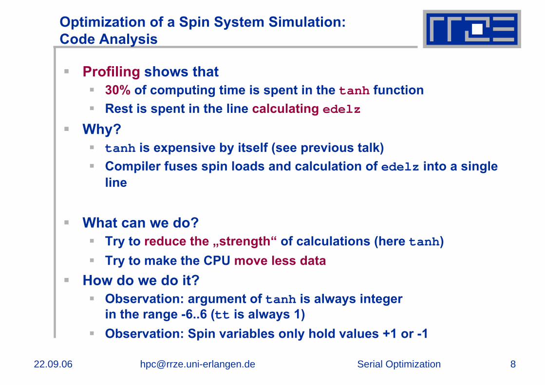
Optimization of a Spin System Simulation:Code Analysis
Profiling shows that30% of computing time is spent in the tanh functionRest is spent in the line calculating edelz
Why?tanh is expensive by itself (see previous talk)Compiler fuses spin loads and calculation of edelz into a singleline
What can we do?Try to reduce the „strength“ of calculations (here tanh)Try to make the CPU move less data
How do we do it?Observation: argument of tanh is always integer in the range -6..6 (tt is always 1)Observation: Spin variables only hold values +1 or -1

22.09.06 [email protected] 9Serial Optimization
Optimization of a Spin System Simulation:Making it Faster
Strength reduction by tabulation of tanh function
BF= 0.5d0*(1.d0+tanh_table(edelz))
Performance increases by 30% as table lookup is done with„lightspeed“ compared to tanh calculation
By declaring spin variables with INTEGER*1 instead of INTEGER*4 the memory requirement is reduced to about ¼
Better cache reuseFactor 2–4 in performance depending on platformWhy don‘t we use just one bit per spin?
Bit operations (mask, shift, add) too expensive → no benefitPotential for a variety of data access optimizations
But: choice of spin must be absolutely random!

22.09.06 [email protected] 10Serial Optimization
Optimization of a Spin System Simulation:Performance Results
0 50 100 150 200 250
Original code
Table +1Byte/Spin
Table +1Bit/Spin
Runtime [sec]
Pentium 4 (2.4 GHz)

General General remarksremarks on on algorithmsalgorithms and and datadata accessaccess

22.09.06 [email protected] 12Serial Optimization
Data access
Data access is the most frequent performance-limiting factor in HPCCache-based microprocessors feature small, fast caches and large, slow memory
“Memory Wall”, “DRAM Gap”Latency can be hidden under certain conditions (prefetch, software pipelining)Bandwidth limit cannot be circumvented
Instead, modify the code to avoid the slow data pathsGeneral guideline: examine “traffic-to-work” ratio (balance) of algorithm to get a hint at possible limitations
Examination of performance-critical loops is vitalImportant metric: (“LOADs/STOREs to FLOPs”)Optimization: lower LDST/FLOP ratio
… and always remember that stride-1 access is best!

22.09.06 [email protected] 13Serial Optimization
“Lightspeed” estimates
How do you know that your code makes good use of theresources? In many cases one can estimate the possible performancelimit (lightspeed) of a loopArchitectural boundary conditions:
Memory bandwidth GWords/s (1 W = 8 bytes)Floating point peak performance GFlops/s
Machine balance
Typical values (memory): 0.13 W/F (Itanium2 1.5 GHz)0.125 W/F (Xeon 3.2 GHz),0.5 W/F (NEC SX8)
]/[ eperformanc FP]/[bandwidth sflops
swordsBm =

22.09.06 [email protected] 14Serial Optimization
“Lightspeed” estimates
Expected performance on the loop level?
Code balance:
Expected fraction of peak performance („lightspeed"):
Example: Vector triad A(:)=B(:)+C(:)*D(:) on 3.2 GHz Xeon
Bm/Bc = 0.125/2 = 0.0625, i.e. 6.25% of peak performance!
Many code optimizations thus aim at lowering Bc
][ operations arithmetic][ (LD/ST) transfer data
flopswordsBc =
c
m
BBl =

22.09.06 [email protected] 15Serial Optimization
Data access – general considerations
Case 1: O(N)/O(N) AlgorithmsO(N) arithmetic operations vs. O(N) data access operationsExamples: Scalar product, vector addition, sparse MVM etc.Performance limited by memory bandwidth for large N(“memory bound”)Limited optimization potential for single loops
at most constant factor for multi-loop operationsExample: successive vector additions
do i=1,Na(i)=b(i)+c(i)
enddo
do i=1,Nz(i)=b(i)+e(i)
enddo no optimization potential for either loop
do i=1,Na(i)=b(i)+c(i)z(i)=b(i)+e(i)
enddo
fusing different loops allows O(N) data reuse from registers
Loop fusion
Bc = 3/1
Bc = 5/2

22.09.06 [email protected] 16Serial Optimization
Data access – general guidelines
Case 2: O(N2)/O(N2) algorithmsExamples: dense matrix-vector multiply, matrix addition, dense matrix transposition etc.
Nested loopsMemory bound for large NSome optimization potential (at most constant factor)
Can often enhance LDST/FLOP ratio by outer loop unrolling
Example: dense matrix-vector multiplication
do i=1,Ndo j=1,Nc(i)=c(i)+a(i,j)*b(j)enddoenddo
= + •
Naïve version loads b[] N times!

22.09.06 [email protected] 17Serial Optimization
Data access – general guidelines
O(N2)/O(N2) algorithms cont’d“Unroll & jam” optimization (or “outer loop unrolling”)
do i=1,Ndo j=1,Nc(i)=c(i)+a(i,j)*b(j)enddoenddo
do i=1,N,2do j=1,Nc(i)=c(i)+a(i,j)*b(j)enddodo j=1,Nc(i+1)=c(i+1)+a(i+1,j)*b(j)enddoenddo
unroll
do i=1,N,2do j=1,Nc(i)=c(i)+a(i,j) * b(j)c(i+1)=c(i+1)+a(i+1,j)* b(j)enddoenddo
jam
b(j) can be reused once from register → save 1 LD operation
Lowered Bc from 1 to 3/4

22.09.06 [email protected] 18Serial Optimization
O(N2)/O(N2) algorithms cont’dData access pattern for 2-way unrolled dense MVM:
Code blance can still be enhanced by more aggressive unrolling (i.e., m-way instead of 2-way)Significant code bloat (try to use compiler directives if possible)
Ultimate limit: b[] only loaded once from memory (Bc ≈ 1/2)Beware: CPU registers are a limited resourceExcessive unrolling can cause register spills to memory
Data access – general guidelines
= + •
Vector b[] now only loadedN/2 times!
Remainder loop handledseparately

OptimizingOptimizing datadata accessaccess forfor densedense matrixmatrix transposetranspose

22.09.06 [email protected] 20Serial Optimization
Simple example for data access problems in cache-based systemsNaïve code:
Problem: Stride-1 access for a implies stride-N access for bAccess to a is perpendicular to cache lines ( )Possibly bad cache efficiency (spatial locality)
Remedy: Outer loop unrolling and blocking
Dense matrix transpose
do i=1,Ndo j=1,Na(j,i) = b(i,j)enddoenddo
a(:,:) b(:,:)

22.09.06 [email protected] 21Serial Optimization
Dense matrix transpose:Vanilla version on different architectures
Second drop; reason?

22.09.06 [email protected] 22Serial Optimization
Dense matrix transpose:Cache thrashing
A closer look (e.g. on Xeon/Netburst) reveals interestingperformance characteristics:
Matrix sizes of powers of 2 seemto be extremely unfortunate
Reason: Cache thrashing!Remedy: Improve effective cachesize by padding the arraydimensions!
a(1024,1024) → a(1025,1025)b(1024,1024) → b(1025,1025)
Eliminates the thrashingcompletely
Rule of thumb: If there is a choice, use dimensions of the form 16•(2k+1)

22.09.06 [email protected] 23Serial Optimization
Dense matrix transpose:Unrolling and blocking
do i=1,Ndo j=1,Na(j,i) = b(i,j)enddoenddo
do i=1,N,Udo j=1,Na(j,i) = b(i,j)a(j,i+1) = b(i+1,j)...a(j,i+U-1) = b(i+U-1,j) enddoenddodo ii=1,N,B
istart=ii; iend=ii+B-1do jj=1,N,Bjstart=jj; jend=jj+B-1do i=istart,iend,Udo j=jstart,jenda(j,i) = b(i,j)a(j,i+1) = b(i+1,j)...a(j,i+U-1) = b(i+U-1,j)
enddo;enddo;enddo;enddo
unroll/jam
blockBlocking and unrolling factors (B,U) can be determined experimentally; be guided by cache sizes and line lengths
22.09.06 [email protected] 24Serial Optimization
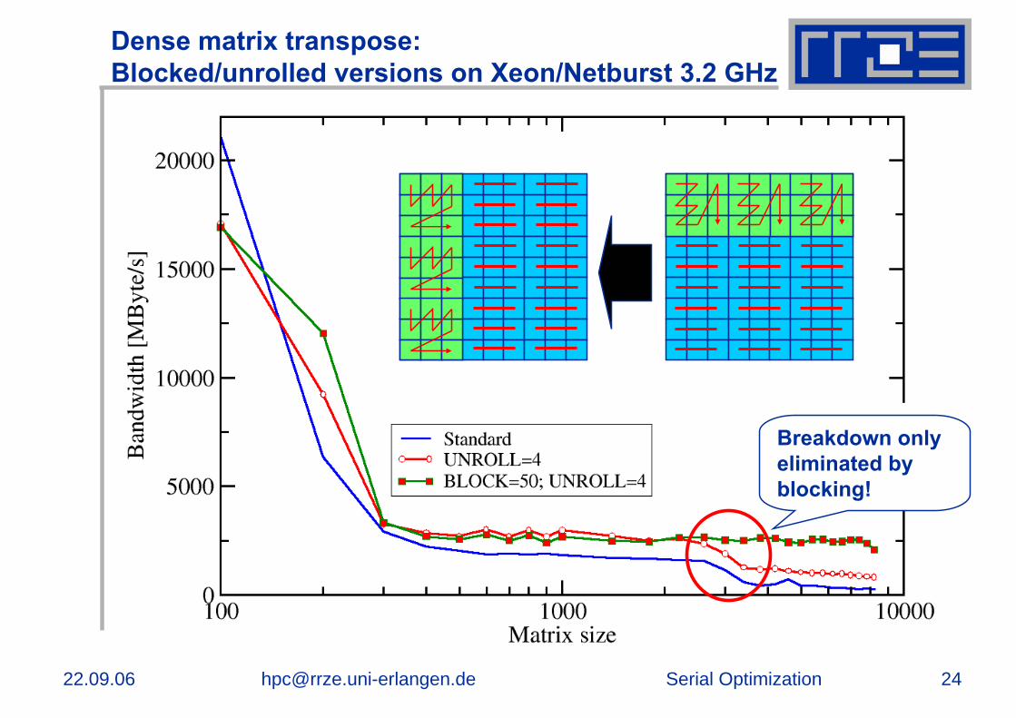
Dense matrix transpose:Blocked/unrolled versions on Xeon/Netburst 3.2 GHz
Breakdown only eliminated by blocking!
22.09.06 [email protected] 25Serial Optimization
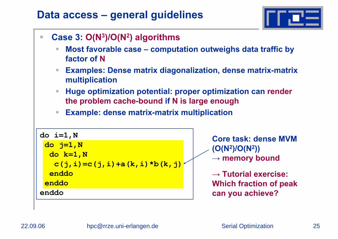
Data access – general guidelines
Case 3: O(N3)/O(N2) algorithmsMost favorable case – computation outweighs data traffic by factor of NExamples: Dense matrix diagonalization, dense matrix-matrix multiplicationHuge optimization potential: proper optimization can render the problem cache-bound if N is large enoughExample: dense matrix-matrix multiplication
do i=1,Ndo j=1,Ndo k=1,Nc(j,i)=c(j,i)+a(k,i)*b(k,j)enddoenddoenddo
Core task: dense MVM (O(N2)/O(N2)) → memory bound
→ Tutorial exercise: Which fraction of peakcan you achieve?

OptimizingOptimizing sparsesparse matrixmatrix--vectorvector multiplicationmultiplication

22.09.06 [email protected] 27Serial Optimization
Sparse matrix-vector multiply (sMVM)
Key ingredient in some matrix diagonalization algorithmsLanczos, Davidson, Jacobi-Davidson
Store only Nnz nonzero elements of matrix and RHS, LHS vectors with Nr (number of matrix rows) entries“Sparse”: Nnz ~ Nr
Type O(N)/O(N) → memory boundNevertheless, there is more than one loop here!
= + • Nr
General case: someindirectaddressingrequired!

22.09.06 [email protected] 28Serial Optimization
Sparse matrix-vector multiply:Different matrix storage schemes
Choice of sparse matrix storage scheme is crucial for performance
Different schemes yield entirely different performance characteristics
Most important formats:CRS (Compressed Row Storage)JDS (Jagged Diagonals Storage)
Other possibilities:CCS (Compressed Column Storage, “Harwell-Boeing”)CDS (Compressed Diagonal Storage)SKS (Skyline Storage)SYDY (Something You Devised Yourself)
Depending on the storage scheme, the memory access patterns differ vastly between the formats
So do the opportunities for optimizationChoose the storage scheme that best fits your needs

22.09.06 [email protected] 29Serial Optimization
…
CRS matrix storage scheme
column indexro
w in
dex
1 2 3 4 …1234…
val[]
1 5 3 72 1 46323 4 21 5 815 … col_idx[]
1 5 15 198 12 … row_ptr[]
val[] stores all the nonzeroes(length Nnz)col_idx[] stores the column index of each nonzero (length Nnz)row_ptr[] stores the starting index of each new row in val[](length: Nr)

22.09.06 [email protected] 30Serial Optimization
CRS sparse MVM
Implement c(:)=m(:,:)*b(:)Only the nonzero elements of the matrix are used
Operation count = 2Nnz
do i = 1,Nrdo j = row_ptr(i), row_ptr(i+1) - 1c(i) = c(i) + val(j) * b(col_idx(j)) enddoenddo
FeaturesLong outer loop (Nr)Probably short inner loop (number of nonzero entries in each respective row)Register-optimized access to result vector c[]Stride-1 access to matrix data in val[]Indexed (indirect) access to RHS vector b[]
22.09.06 [email protected] 31Serial Optimization
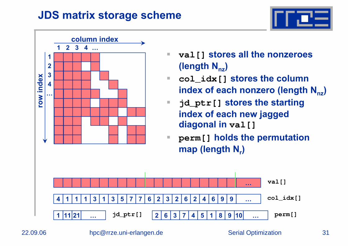
JDS matrix storage scheme
…
column indexro
w in
dex
1 2 3 4 …1234…
4 3 2 21 3 36711 7 26 4 651 … col_idx[]9 9
val[]
1 11 21 … jd_ptr[] 2 16 4 953 1087 … perm[]
val[] stores all the nonzeroes(length Nnz)col_idx[] stores the column index of each nonzero (length Nnz)jd_ptr[] stores the starting index of each new jagged diagonal in val[]perm[] holds the permutation map (length Nr)
22.09.06 [email protected] 32Serial Optimization
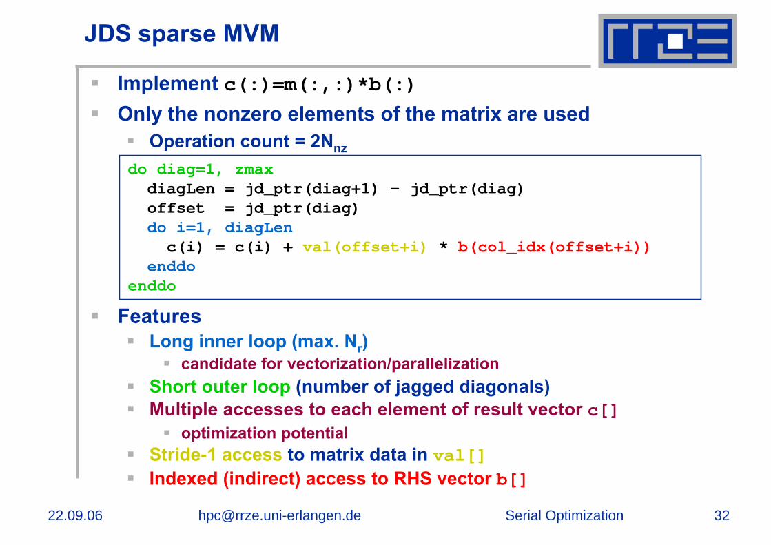
JDS sparse MVM
Implement c(:)=m(:,:)*b(:)Only the nonzero elements of the matrix are used
Operation count = 2Nnz
do diag=1, zmaxdiagLen = jd_ptr(diag+1) - jd_ptr(diag)offset = jd_ptr(diag)do i=1, diagLen
c(i) = c(i) + val(offset+i) * b(col_idx(offset+i))enddo
enddo
FeaturesLong inner loop (max. Nr)
candidate for vectorization/parallelizationShort outer loop (number of jagged diagonals)Multiple accesses to each element of result vector c[]
optimization potentialStride-1 access to matrix data in val[]Indexed (indirect) access to RHS vector b[]
22.09.06 [email protected] 33Serial Optimization
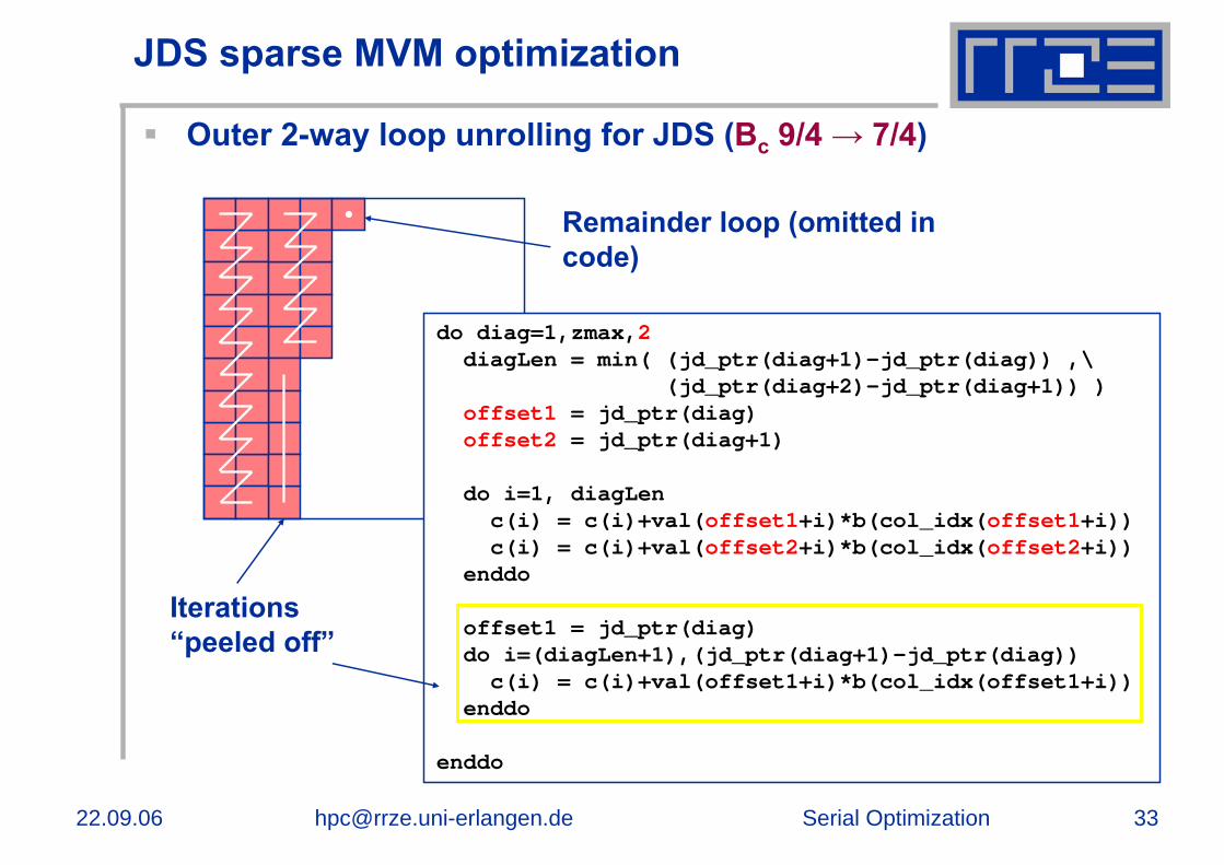
JDS sparse MVM optimization
Outer 2-way loop unrolling for JDS (Bc 9/4 → 7/4)
do diag=1,zmax,2diagLen = min( (jd_ptr(diag+1)-jd_ptr(diag)) ,\
(jd_ptr(diag+2)-jd_ptr(diag+1)) )offset1 = jd_ptr(diag) offset2 = jd_ptr(diag+1)
do i=1, diagLenc(i) = c(i)+val(offset1+i)*b(col_idx(offset1+i))c(i) = c(i)+val(offset2+i)*b(col_idx(offset2+i))
enddo
offset1 = jd_ptr(diag) do i=(diagLen+1),(jd_ptr(diag+1)-jd_ptr(diag))c(i) = c(i)+val(offset1+i)*b(col_idx(offset1+i))
enddo
enddo
Iterations“peeled off”
Remainder loop (omitted in code)
22.09.06 [email protected] 34Serial Optimization
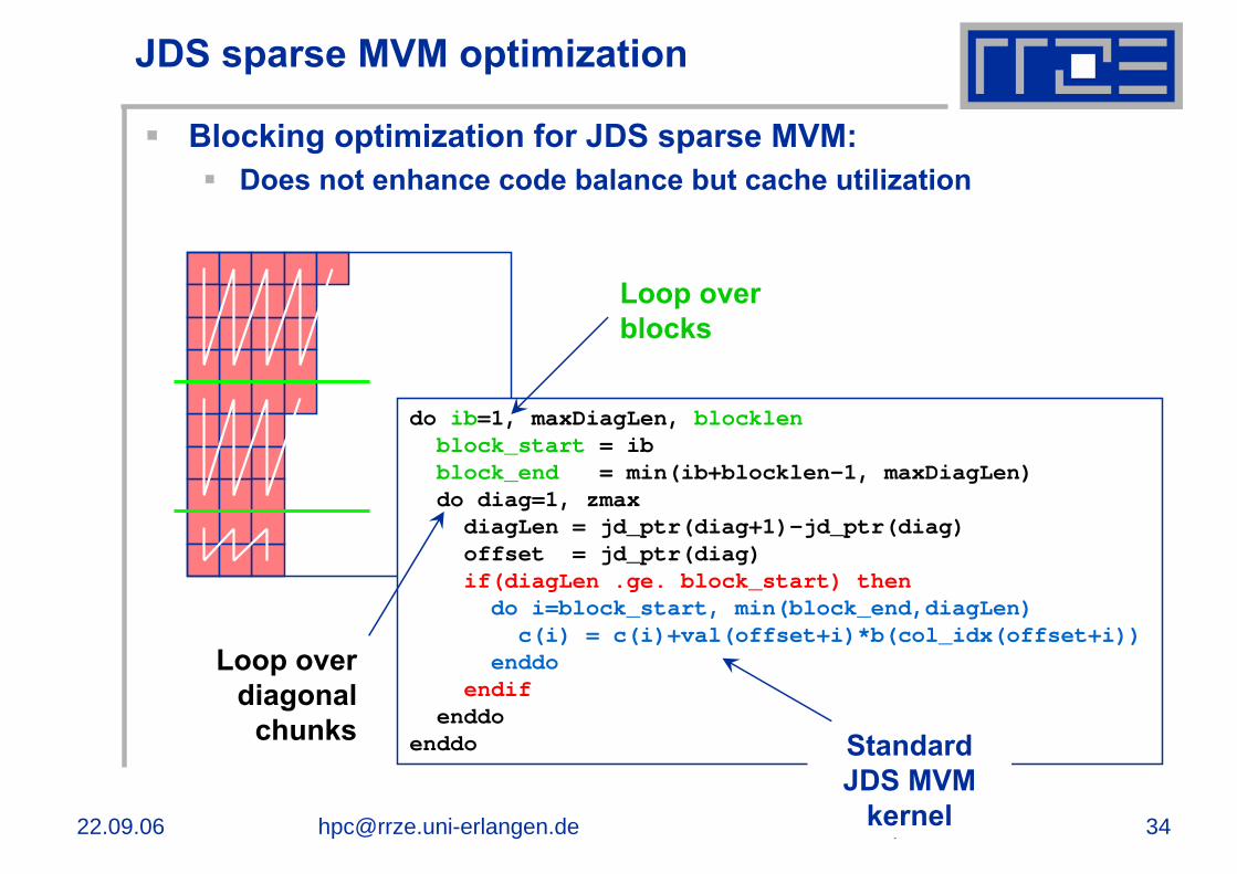
JDS sparse MVM optimization
Blocking optimization for JDS sparse MVM:Does not enhance code balance but cache utilization
do ib=1, maxDiagLen, blocklenblock_start = ibblock_end = min(ib+blocklen-1, maxDiagLen)do diag=1, zmaxdiagLen = jd_ptr(diag+1)-jd_ptr(diag)offset = jd_ptr(diag)if(diagLen .ge. block_start) thendo i=block_start, min(block_end,diagLen)c(i) = c(i)+val(offset+i)*b(col_idx(offset+i))
enddoendif
enddoenddo
Loop overblocks
Loop overdiagonal
chunks Standard JDS MVM
kernel
22.09.06 [email protected] 35Serial Optimization
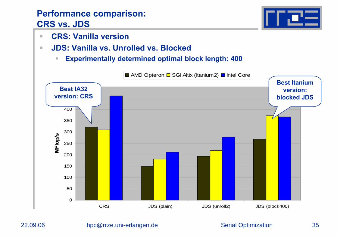
Performance comparison:CRS vs. JDS
CRS: Vanilla versionJDS: Vanilla vs. Unrolled vs. Blocked
Experimentally determined optimal block length: 400
0
50
100
150
200
250
300
350
400
450
500
CRS JDS (plain) JDS (unroll2) JDS (block400)
MFl
op/s
AMD Opteron SGI Altix (Itanium2) Intel CoreBest Itanium
version: blocked JDS
Best IA32 version: CRS

22.09.06 [email protected] 36Serial Optimization
Performance comparison:Real programmers use vector computers…
0
500
1000
1500
2000
2500
3000
3500
CRS JDS (plain) JDS (unroll2) JDS (block400)
MFl
op/s
AMD Opteron SGI Altix (Itanium2) Intel Core NEC SX-8

22.09.06 [email protected] 37Serial Optimization
References
S. Goedecker, A. HoisiePerformance Optimization of Numerically Intensive CodesSociety for Industrial & Applied Mathematics,U.S. (ISBN 0898714842)
R. Gerber et al.The Software Optimization Cookbook, Second EditionHigh-Performance Recipes for IA-32 PlatformsIntel Press (ISBN 0-9764832-1-1)
R. Barrett et al.Templates for the Solution of Linear Systems: Building Blocks for Iterative Methodshttp://www.netlib.org/templates/Templates.html