Fuzzy inventory model with exponential demand …Fuzzy inventory model with exponential demand......
18
Global Journal of Pure and Applied Mathematics. ISSN 0973-1768 Volume 12, Number 3 (2016), pp. 2573–2589 © Research India Publications http://www.ripublication.com/gjpam.htm Fuzzy inventory model with exponential demand and time-varying deterioration N.K. Sahoo Dept. of Math., S.S.S. Mahavidyalaya, Goudakateni, Dhenkanal-759001. E-mail: [email protected] Bhabani S. Mohanty and P.K. Tripathy P.G. Dept. of Statistics, Utkal University,Vanivihar, Bhubaneswar - 751004 E-mail: [email protected], [email protected] Abstract This paper investigates with the development of a fuzzy inventory model with time-varying demand, deterioration and salvage. The deterioration rate, demand, holding cost, unit cost and salvage value are taken as trapezoidal fuzzy numbers. Both graded mean integration and signed distance method are used to defuzzify the total cost function. Numerical examples are given to validate the proposed mathematical model which has been developed for determining the optimal order quantity, optimal cycle time and optimal total inventory cost. Sensitivity analysis is also carried out to explore the effect of changes in the optimal solution with respect to change in various parameters. AMS subject classification: Keywords: Trapezoidal fuzzy number, Defuzzification, Salvage. 1. Introduction During the last decade, many researchers have studied inventory models for deteriorating items such as medicines, blood, electronic items and fashion cosmetics etc. The analysis
Transcript of Fuzzy inventory model with exponential demand …Fuzzy inventory model with exponential demand......
Global Journal of Pure and Applied Mathematics.ISSN 0973-1768 Volume 12, Number 3 (2016), pp. 2573–2589© Research India Publicationshttp://www.ripublication.com/gjpam.htm
Fuzzy inventory model with exponential demand andtime-varying deterioration
N.K. Sahoo
Dept. of Math.,S.S.S. Mahavidyalaya,
Goudakateni, Dhenkanal-759001.E-mail: [email protected]
Bhabani S. Mohanty and P.K. Tripathy
P.G. Dept. of Statistics,Utkal University,Vanivihar,
Bhubaneswar - 751004E-mail: [email protected],
Abstract
This paper investigates with the development of a fuzzy inventory model withtime-varying demand, deterioration and salvage. The deterioration rate, demand,holding cost, unit cost and salvage value are taken as trapezoidal fuzzy numbers.Both graded mean integration and signed distance method are used to defuzzifythe total cost function. Numerical examples are given to validate the proposedmathematical model which has been developed for determining the optimal orderquantity, optimal cycle time and optimal total inventory cost. Sensitivity analysis isalso carried out to explore the effect of changes in the optimal solution with respectto change in various parameters.
AMS subject classification:Keywords: Trapezoidal fuzzy number, Defuzzification, Salvage.
1. Introduction
During the last decade, many researchers have studied inventory models for deterioratingitems such as medicines, blood, electronic items and fashion cosmetics etc. The analysis

2574 N.K. Sahoo, et al.
of deteriorating inventory models began with Ghare and Schrader [3] who developedEOQ model with a constant rate of deterioration. Since then, many related researchcould be found in Hariga [4], Heng et al. [5], Hollier and Mak [6], Jaggi, Aggarwaland Goel [8], Moon et al. [12], Sarker et al. [14], and Wee [16]. On the other hand,the traditional EOQ models do not cover the effect of salvage value, which cannot beignored now due to piling of materials leading to salvage. Such a situation will motivatethe procurement planner to accumulate revenue and earn a payoff. So Mishra et al. [11]has proposed a more realistic collaborative inventory model for deteriorating items withsalvage value.
One of the weaknesses of current inventory model which is widely applied in businessworld is the unrealistic assumption of the different parameters. Bellan and Zadeh [1] firstintroduced the fuzzy set theory in decision making process. Zadeh ([20], [21]) showedthat for the new products and seasonal items it is better to use fuzzy numbers thanprobabilistic approaches. The uncertainties are shown to be captured by several articlesby Chang, Yao & Lee [2] and Yao & Lee [18] and Yao & Chiang [17]. There have beensystematic progresses in the development of inventory models from crisp parameters tofuzzy parameters. Park [13] and Vujosevic et al. [15] improved the inventory models infuzzy sense in which ordering cost and holding cost are represented by Fuzzy numbers.Park has represented the cost as trapezoidal numbers, whileVujosevic et al. has discussedthe ordering cost by triangular fuzzy number and the holding cost by trapezoidal fuzzynumber. LaterYao & Lee [19], Kao & Hsu [10], Hsieh [7], Jaggi et al. [9] have developedinventory models by taking major parameters as fuzzy for defuzzifying the fuzzy totalinventory cost.
In this paper it has presented as fuzzy inventory model with time-varying demandand deterioration with salvage value, in which the major costs are considered as fuzzynumbers. The trapezoidal type fuzzy number is used for representing fuzzy numbers.Defuzzification is done using both Graded Mean Integration Method and Signed DistanceMethod. The optimal costs are obtained in crisp as well as fuzzy model. The resultsobtained by two methods are compared.
2. Preliminaries
A fuzzy set X on the given universal set is a set of order pairs A = {(x, µA(x)) : x ∈ X},where µA : X → [0, 1] is called membership function.
The α-cut of A is defined by
Aα = {x : µA(x) = α, α ≥ 0}If R is a real line, then a fuzzy number is a fuzzy set A with membership functionµA : X → [0, 1], having the following properties
(i) A is normal i.e. there exist x ∈ R such that µA(x) = 1
(ii) A is piecewise continuous.
Fuzzy inventory model with exponential demand... 2575
(iii) sup p(A) = cl{x ∈ R : µA(x) > 0}, where cl represents the closure of a set.
(iv) A is a convex fuzzy set.
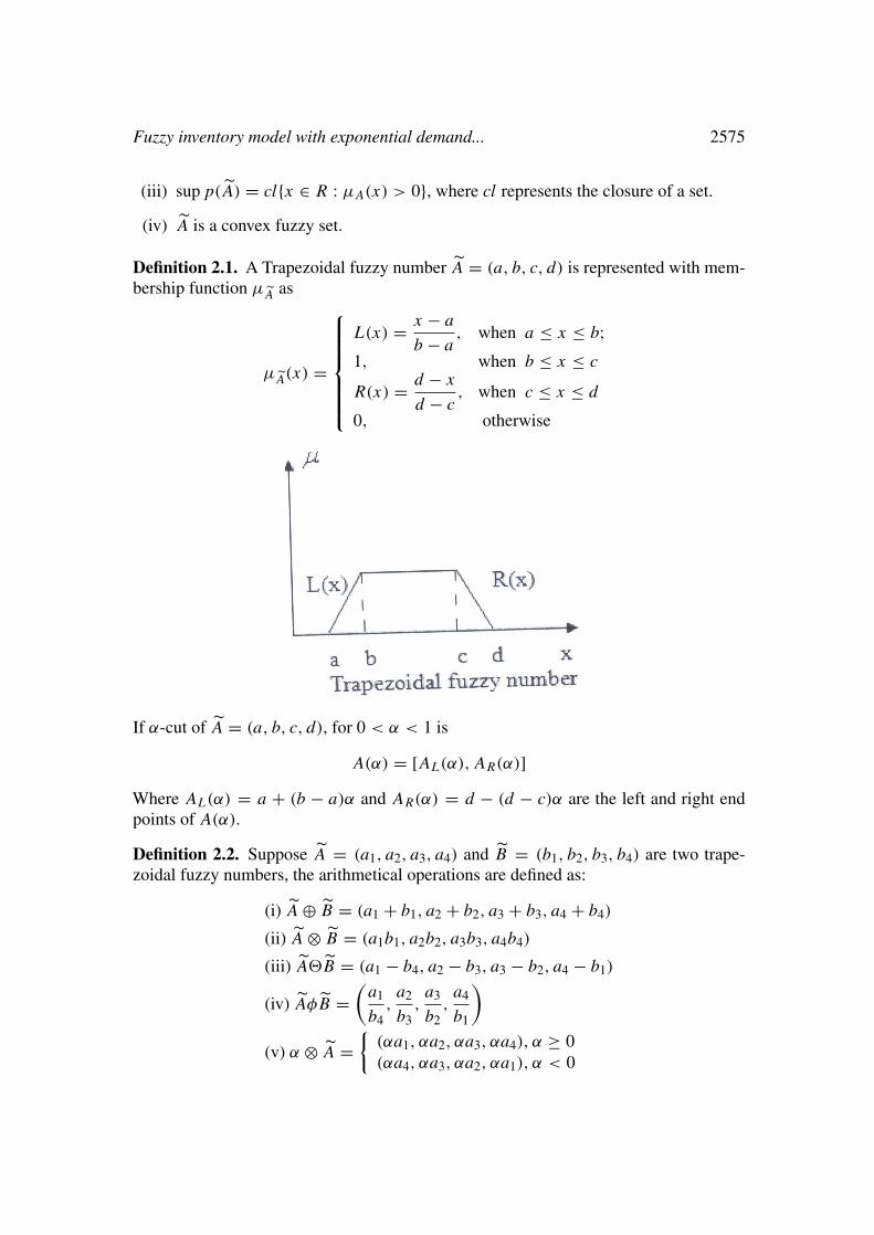
Definition 2.1. A Trapezoidal fuzzy number A = (a, b, c, d) is represented with mem-bership function µA as
µA(x) =
L(x) = x − a
b − a, when a ≤ x ≤ b;
1, when b ≤ x ≤ c
R(x) = d − x
d − c, when c ≤ x ≤ d
0, otherwise
If α-cut of A = (a, b, c, d), for 0 < α < 1 is
A(α) = [AL(α), AR(α)]Where AL(α) = a + (b − a)α and AR(α) = d − (d − c)α are the left and right endpoints of A(α).
Definition 2.2. Suppose A = (a1, a2, a3, a4) and B = (b1, b2, b3, b4) are two trape-zoidal fuzzy numbers, the arithmetical operations are defined as:
(i) A ⊕ B = (a1 + b1, a2 + b2, a3 + b3, a4 + b4)
(ii) A ⊗ B = (a1b1, a2b2, a3b3, a4b4)
(iii) A�B = (a1 − b4, a2 − b3, a3 − b2, a4 − b1)
(iv) AφB =(
a1
b4,a2
b3,a3
b2,a4
b1
)
(v) α ⊗ A ={
(αa1, αa2, αa3, αa4), α ≥ 0(αa4, αa3, αa2, αa1), α < 0

2576 N.K. Sahoo, et al.
Definition 2.3. Let A = (a, b, c, d) be a trapezoidal fuzzy number, then the GradedMean Integration Method of A is defined as
P(A) =1
2
∫ 1
0α[AL(α) + AR(α)]dα∫ 1
0 α dα
= a + 2b + 2c + d
6
Definition 2.4. Let A = (a, b, c, d) be a fuzzy set defined on R. Then the SignedDistance Method of A is defined as
d(A, 0) = 1
2
∫ 1
0[AL(α) + AR(α)]dα
= a + b + c + d
4
3. Assumptions and Notation
i. R(t) = aebt where a, b > 0, a >> b is the demand rate at any time t .
ii. The replenishment rate is infinite.
iii. The lead time is zero and shortages are not allowed.
iv. A is the ordering cost per order.
v. C is the purchase cost per units.
v. C is the purchase cost per units.
vi. h(t) = h + αt, h > 0, α > 0 is the holding cost per unit time.
vii. θ(t) = θt, 0 < θ < 1, where θ is the rate of deterioration.
viii. The salvage value βC(0 ≤ β ≤ 1) is associated to deteriorated units during thecycle time.
ix. The deteriorated units cannot be repaired or replaced during the period underreview.
x. K(t) is the total inventory cost.
xi. R is the fuzzy demand.
xii. θ is the fuzzy deterioration rate.
Fuzzy inventory model with exponential demand... 2577
xiii. h is the fuzzy holding cost.
xiv. C is the fuzzy purchase cost.
xv. βC is the fuzzy salvage value.
xvi. K(t) is the total fuzzy inventory cost per unit time.
xvii. KdG(T ) is the defuzzify value of K(T ) by applying Graded Mean IntegrationMethod.
xviii. Kds(T ) is the defuzzify value of K(T ) by applying Signed Distance Method.
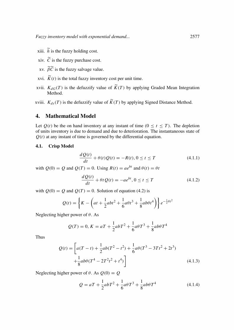
4. Mathematical Model
Let Q(t) be the on hand inventory at any instant of time (0 ≤ t ≤ T ). The depletionof units inventory is due to demand and due to deterioration. The instantaneous state ofQ(t) at any instant of time is governed by the differential equation.
4.1. Crisp Model
dQ(t)
dt+ θ(t)Q(t) = −R(t), 0 ≤ t ≤ T (4.1.1)
with Q(0) = Q and Q(T ) = 0. Using R(t) = aebt and θ(t) = θt
dQ(t)
dt+ θtQ(t) = −aebt , 0 ≤ t ≤ T (4.1.2)
with Q(0) = Q and Q(T ) = 0. Solution of equation (4.2) is
Q(t) ={K −
(at + 1
2abt2 + 1
6aθt3 + 1
8abθt4
)}e− 1
2 θt2
Neglecting higher power of θ . As
Q(T ) = 0, K = aT + 1
2abT 2 + 1
6aθT 3 + 1
8abθT 4
Thus
Q(t) =[a(T − t) + 1
2ab(T 2 − t2) + 1
6aθ(T 3 − 3T t2 + 2t3)
+1
8abθ(T 4 − 2T 2t2 + t4)
](4.1.3)
Neglecting higher power of θ . As Q(0) = Q
Q = aT + 1
2abT 2 + 1
6aθT 3 + 1
8abθT 4 (4.1.4)

2578 N.K. Sahoo, et al.
The total cost per time unit T C(T ) is given by
T C(T ) = 1
T(IHC + OC + CD − SV ) (4.1.5)
Where
(i) IHC = Inventory holding cost
=∫ T
0h(t)Q(t)dt
= 1
2ahT 2 + 1
3abhT 3 + 1
12aθhT 4 + 1
15abθhT 5 + 1
6aαT 3
+ 1
8abαT 4 + 1
40aθαT 5 + 1
48abθαT 6
(ii) OC = ordering cost = A
(iii) CD = Cost due to Deterioration
= C
[Q −
∫ T
0R(t)dt
]
= 1
6CaθT 3 + 1
8CabθT 4
(iv) SV = Salvage value of Deterioration items
βC
[Q −
∫ T
0R(t)dt
]
= 1
6βCaθT 3 + 1
8βCabθT 4
Thus,
T C(T ) =
A + 1
2ahT 2 + 1
3abhT 3 + 1
12aθhT 4 + 1
15abθhT 5
+1
6aαT 3 + 1
8abαT 4 + 1
40aθαT 5 + 1
48abθαT 6
+1
6CaθT 3 + 1
8CabθT 4 − 1
6βCaθT 3 − 1
8βCabθT 4
(4.1.6)

Fuzzy inventory model with exponential demand... 2579
4.2. Fuzzy Model
Let
a = (a1, a2, a3, a4), b = (b1, b2, b3, b4),
h = (h1, h2, h3, h4), α = (α1, α2, α3, α4),
θ = (θ1, θ2, θ3, θ4),
β = (β1, β2, β3, β4),
C = (C1, C2, C3, C4)
are as trapezoidal fuzzy number. Total cost of the system per unit time in fuzzy sense isgiven by
T C(T ) = 1
T
A + 1
2ahT 2 + 1
3ab hT 3 + 1
12aθ hT 4 + 1
15ab θ hT 5
+1
6aαT 3 + 1
8abαT 4 + 1
40aθ αT 5 + 1
48abθ αT 6
+1
6CaθT 3 + 1
8CabθT 4 − 1
6βCaθT 3 − 1
8βCabθT 4
(4.2.1)
we defuzzify the fuzzy total cost T C(T ) by Graded Mean Integration and Signed Dis-tance Method.(i) By Graded Mean Integration Method, Total Cost is given by
T CGM(T ) = 1
6
[T CGM1(T ) + 2T CGM2(T ) + 2T CGM3(T ) + T CGM4(T )
]Where
T CGM1(T ) = 1
T
A + 1
2a1h1T
2 + 1
3a1b1h1T
3 + 1
12a1θ1h1T
4 + 1
15a1b1θ1h1T
5
+1
6a1α1T
3 + 1
8a1b1α1T
4 + 1
40a1θ1α1T
5 + 1
48a1b1θ1α1T
6
+1
6C1a1θ1T
3 + 1
8C1a1b1θ1T
4 − 1
6β1C1a1θ1T
3
−1
8β1C1a1b1θ1T
4
T CGM2(T ) = 1
T
A + 1
2a2h2T
2 + 1
3a2b2h2T
3 + 1
12a2θ2h2T
4 + 1
15a2b2θ2h2T
5
+1
6a2α2T
3 + 1
8a2b2α2T
4 + 1
40a2θ2α2T
5 + 1
48a2b2θ2α2T
6
+1
6C2a2θ2T
3 + 1
8C2a2b2θ2T
4 − 1
6β2C2a2θ2T
3
−1
8β2C2a2b2θ2T
4
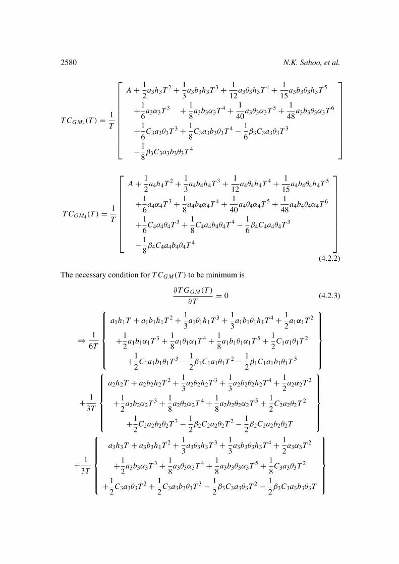
2580 N.K. Sahoo, et al.
T CGM3(T ) = 1
T
A + 1
2a3h3T
2 + 1
3a3b3h3T
3 + 1
12a3θ3h3T
4 + 1
15a3b3θ3h3T
5
+1
6a3α3T
3 + 1
8a3b3α3T
4 + 1
40a3θ3α3T
5 + 1
48a3b3θ3α3T
6
+1
6C3a3θ3T
3 + 1
8C3a3b3θ3T
4 − 1
6β3C3a3θ3T
3
−1
8β3C3a3b3θ3T
4
T CGM4(T ) = 1
T
A + 1
2a4h4T
2 + 1
3a4b4h4T
3 + 1
12a4θ4h4T
4 + 1
15a4b4θ4h4T
5
+1
6a4α4T
3 + 1
8a4b4α4T
4 + 1
40a4θ4α4T
5 + 1
48a4b4θ4α4T
6
+1
6C4a4θ4T
3 + 1
8C4a4b4θ4T
4 − 1
6β4C4a4θ4T
3
−1
8β4C4a4b4θ4T
4
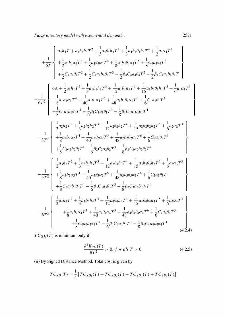
(4.2.2)
The necessary condition for T CGM(T ) to be minimum is
∂T GGM(T )
∂T= 0 (4.2.3)
⇒ 1
6T
a1h1T + a1b1h1T2 + 1
3a1θ1h1T
3 + 1
3a1b1θ1h1T
4 + 1
2a1α1T
2
+1
2a1b1α1T
3 + 1
8a1θ1α1T
4 + 1
8a1b1θ1α1T
5 + 1
2C1a1θ1T
2
+1
2C1a1b1θ1T
3 − 1
2β1C1a1θ1T
2 − 1
2β1C1a1b1θ1T
3
+ 1
3T
a2h2T + a2b2h2T2 + 1
3a2θ2h2T
3 + 1
3a2b2θ2h2T
4 + 1
2a2α2T
2
+1
2a2b2α2T
3 + 1
8a2θ2α2T
4 + 1
8a2b2θ2α2T
5 + 1
2C2a2θ2T
2
+1
2C2a2b2θ2T
3 − 1
2β2C2a2θ2T
2 − 1
2β2C2a2b2θ2T
+ 1
3T
a3h3T + a3b3h1T2 + 1
3a3θ3h3T
3 + 1
3a3b3θ3h3T
4 + 1
2a3α3T
2
+1
2a3b3α3T
3 + 1
8a3θ3α3T
4 + 1
8a3b3θ3α3T
5 + 1
8C3a3θ3T
2
+1
2C3a3θ3T
2 + 1
2C3a3b3θ3T
3 − 1
2β3C3a3θ3T
2 − 1
2β3C3a3b3θ3T
Fuzzy inventory model with exponential demand... 2581
+ 1
6T
a4h4T + a4b4h4T2 + 1
3a4θ4h4T
3 + 1
3a4b4θ4h4T
4 + 1
2a4α4T
2
+1
2a4b4α4T
3 + 1
8a4θ4α4T
4 + 1
8a4b4θ4α4T
5 + 1
8C4a4θ4T
2
+1
2C4a4θ4T
2 + 1
2C4a4b4θ4T
3 − 1
2β4C4a4θ4T
2 − 1
2β4C4a4b4θ4T
− 1
6T 2
6A + 1
2a1h1T
2 + 1
3a1b1h1T
3 + 1
12a1θ1h1T
4 + 1
15a1b1θ1h1T
5 + 1
6a1α1T
3
+1
8a1b1α1T
4 + 1
40a1θ1α1T
5 + 1
48a1b1θ1α1T
6 + 1
6C1a1θ1T
3
+1
8C1a1b1θ1T
4 − 1
6β1C1a1θ1T
3 − 1
8β1C1a1b1θ1T
4
− 1
3T 2
1
2a2h2T
2 + 1
3a2b2h2T
3 + 1
12a2θ2h2T
4 + 1
15a2b2θ2h2T
5 + 1
6a2α2T
3
+1
8a2b2α2T
4 + 1
40a2θ2α2T
5 + 1
48a2b2θ2α2T
6 + 1
6C2a2θ2T
3
+1
8C2a2b2θ2T
4 − 1
6β2C2a2θ2T
3 − 1
8β2C2a2b2θ2T
4
− 1
3T 2
1
2a3h3T
2 + 1
3a3b3h3T
3 + 1
12a3θ3h3T
4 + 1
15a3b3θ3h3T
5 + 1
6a3α3T
3
+1
8a3b3α3T
4 + 1
40a3θ3α3T
5 + 1
48a3b3θ3α3T
6 + 1
6C3a3θ3T
3
+1
8C3a3b3θ3T
4 − 1
6β3C3a3θ3T
3 − 1
8β3C3a3b3θ3T
4
− 1
6T 2
1
2a4h4T
2 + 1
3a4b4h4T
3 + 1
12a4θ4h4T
4 + 1
15a4b4θ4h4T
5 + 1
6a4α4T
3
+1
8a4b4α4T
4 + 1
40a4θ4α4T
5 + 1
48a4b4θ4α4T
6 + 1
6C4a4θ4T
3
+1
8C4a4b4θ4T
4 − 1
6β4C4a4θ4T
3 − 1
8β4C4a4b4θ4T
4
(4.2.4)T CGM(T ) is minimum only if
∂2KdG(T )
∂T 2> 0, f or all T > 0. (4.2.5)
(ii) By Signed Distance Method, Total cost is given by
T CSD(T ) = 1
4
[T CSD1(T ) + T CSD2(T ) + T CSD3(T ) + T CSD4(T )
]

2582 N.K. Sahoo, et al.
Where
T CSD1(T ) = 1
T
A + 1
2a1h1T
2 + 1
3a1b1h1T
3 + 1
12a1θ1h1T
4 + 1
15a1b1θ1h1T
5
+1
6a1α1T
3 + 1
8a1b1α1T
4 + 1
40a1θ1α1T
5 + 1
48a1b1θ1α1T
6
+1
6C1a1θ1T
3 + 1
8C1a1b1θ1T
4 − 1
6β1C1a1θ1T
3 − 1
8β1C1a1b1θ1T
4
T CSD2(T ) = 1
T
A + 1
2a2h2T
2 + 1
3a2b2h2T
3 + 1
12a2θ2h2T
4 + 1
15a2b2θ2h2T
5
+1
6a2α2T
3 + 1
8a2b2α2T
4 + 1
40a2θ2α2T
5 + 1
48a2b2θ2α2T
6
+1
6C2a2θ2T
3 + 1
8C2a2b2θ2T
4 − 1
6β2C2a2θ2T
3 − 1
8β2C2a2b2θ2T
4
T CSD3(T ) = 1
T
A + 1
2a3h3T
2 + 1
3a3b3h3T
3 + 1
12a3θ3h3T
4 + 1
15a3b3θ3h3T
5
+1
6a3α3T
3 + 1
8a3b3α3T
4 + 1
40a3θ3α3T
5 + 1
48a3b3θ3α3T
6
+1
6C3a3θ3T
3 + 1
8C3a3b3θ3T
4 − 1
6β3C3a3θ3T
3 − 1
8β3C3a3b3θ3T
4
T CSD4(T ) = 1
T
A + 1
2a4h4T
2 + 1
3a4b4h4T
3 + 1
12a4θ4h4T
4 + 1
15a4b4θ4h4T
5
+1
6a4α4T
3 + 1
8a4b4α4T
4 + 1
40a4θ4α4T
5 + 1
48a4b4θ4α4T
6
+1
6C4a4θ4T
3 + 1
8C4a4b4θ4T
4 − 1
6β4C4a4θ4T
3 − 1
8β4C4a4b4θ4T
4
(4.2.6)
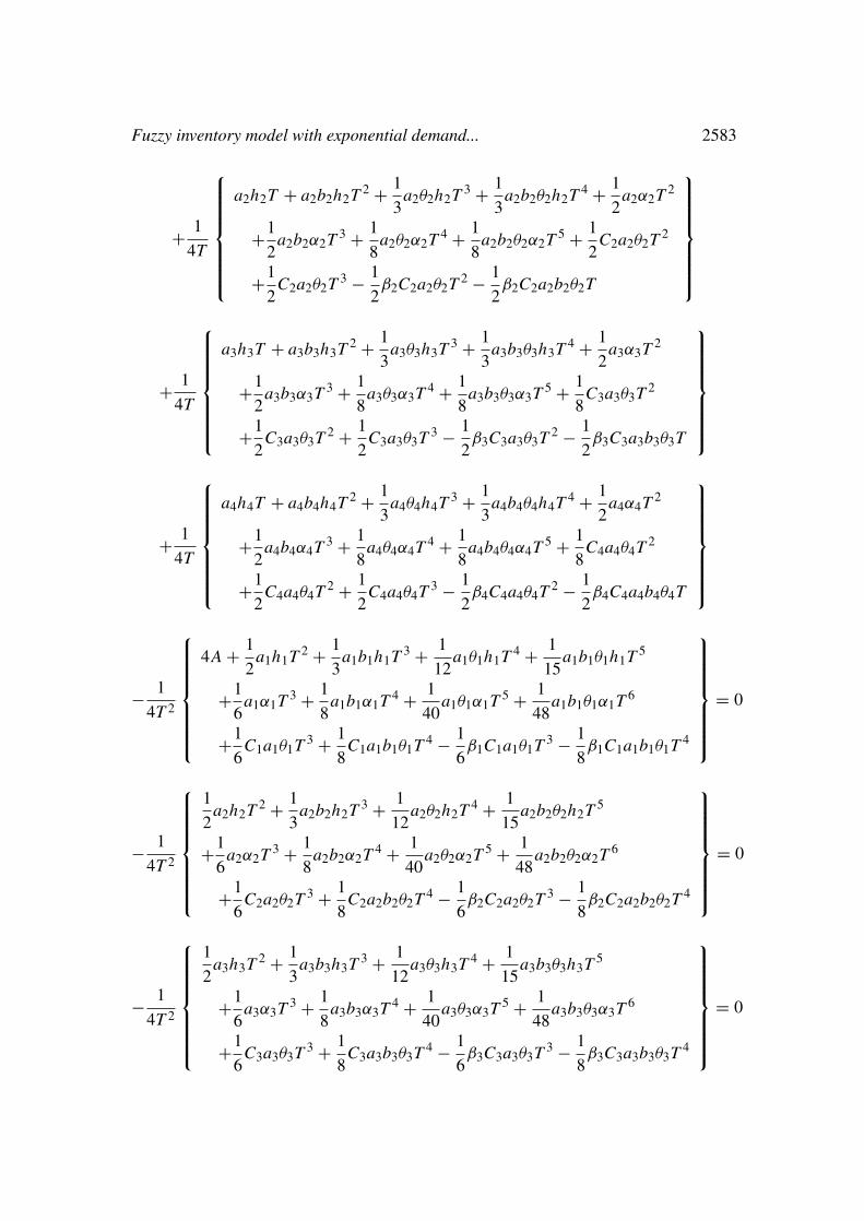
The necessary condition for T CSD(T ) to be minimum is
∂T CSD(T )
∂T= 0 (4.2.7)
⇒ 1
4T
a1h1T + a1b1h1T2 + 1
3a1θ1h1T
3 + 1
3a1b1θ1h1T
4 + 1
2a1α1T
2
+1
2a1b1α1T
3 + 1
8a1θ1α1T
4 + 1
8a1b1θ1α1T
5 + 1
2C1a1θ1T
2
+1
2C1a1θ1T
3 − 1
2β1C1a1θ1T
2 − 1
2β1C1a1b1θ1T
Fuzzy inventory model with exponential demand... 2583
+ 1
4T
a2h2T + a2b2h2T2 + 1
3a2θ2h2T
3 + 1
3a2b2θ2h2T
4 + 1
2a2α2T
2
+1
2a2b2α2T
3 + 1
8a2θ2α2T
4 + 1
8a2b2θ2α2T
5 + 1
2C2a2θ2T
2
+1
2C2a2θ2T
3 − 1
2β2C2a2θ2T
2 − 1
2β2C2a2b2θ2T
+ 1
4T
a3h3T + a3b3h3T2 + 1
3a3θ3h3T
3 + 1
3a3b3θ3h3T
4 + 1
2a3α3T
2
+1
2a3b3α3T
3 + 1
8a3θ3α3T
4 + 1
8a3b3θ3α3T
5 + 1
8C3a3θ3T
2
+1
2C3a3θ3T
2 + 1
2C3a3θ3T
3 − 1
2β3C3a3θ3T
2 − 1
2β3C3a3b3θ3T
+ 1
4T
a4h4T + a4b4h4T2 + 1
3a4θ4h4T
3 + 1
3a4b4θ4h4T
4 + 1
2a4α4T
2
+1
2a4b4α4T
3 + 1
8a4θ4α4T
4 + 1
8a4b4θ4α4T
5 + 1
8C4a4θ4T
2
+1
2C4a4θ4T
2 + 1
2C4a4θ4T
3 − 1
2β4C4a4θ4T
2 − 1
2β4C4a4b4θ4T
− 1
4T 2
4A + 1
2a1h1T
2 + 1
3a1b1h1T
3 + 1
12a1θ1h1T
4 + 1
15a1b1θ1h1T
5
+1
6a1α1T
3 + 1
8a1b1α1T
4 + 1
40a1θ1α1T
5 + 1
48a1b1θ1α1T
6
+1
6C1a1θ1T
3 + 1
8C1a1b1θ1T
4 − 1
6β1C1a1θ1T
3 − 1
8β1C1a1b1θ1T
4
= 0
− 1
4T 2
1
2a2h2T
2 + 1
3a2b2h2T
3 + 1
12a2θ2h2T
4 + 1
15a2b2θ2h2T
5
+1
6a2α2T
3 + 1
8a2b2α2T
4 + 1
40a2θ2α2T
5 + 1
48a2b2θ2α2T
6
+1
6C2a2θ2T
3 + 1
8C2a2b2θ2T
4 − 1
6β2C2a2θ2T
3 − 1
8β2C2a2b2θ2T
4
= 0
− 1
4T 2
1
2a3h3T
2 + 1
3a3b3h3T
3 + 1
12a3θ3h3T
4 + 1
15a3b3θ3h3T
5
+1
6a3α3T
3 + 1
8a3b3α3T
4 + 1
40a3θ3α3T
5 + 1
48a3b3θ3α3T
6
+1
6C3a3θ3T
3 + 1
8C3a3b3θ3T
4 − 1
6β3C3a3θ3T
3 − 1
8β3C3a3b3θ3T
4
= 0
2584 N.K. Sahoo, et al.
− 1
4T 2
1
2a4h4T
2 + 1
3a4b4h4T
3 + 1
12a4θ4h4T
4 + 1
15a4b4θ4h4T
5
+1
6a4α4T
3 + 1
8a4b4α4T
4 + 1
40a4θ4α4T
5 + 1
48a4b4θ4α4T
6
+1
6C4a4θ4T
3 + 1
8C4a4b4θ4T
4 − 1
6β4C4a4θ4T
3 − 1
8β4C4a4b4θ4T
4
= 0
(4.2.8)T CSD(T ) is minimum only if
∂2KdG(T )
∂T 2> 0, f or all T > 0. (4.2.9)
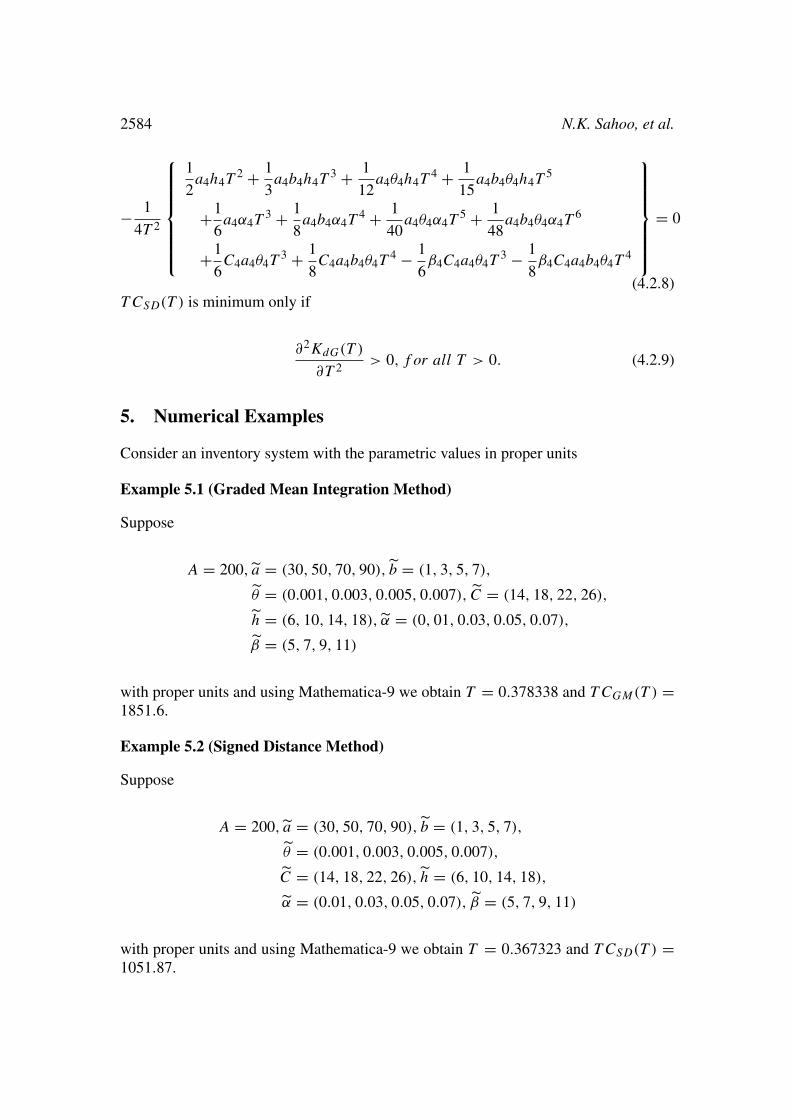
5. Numerical Examples
Consider an inventory system with the parametric values in proper units
Example 5.1 (Graded Mean Integration Method)
Suppose
A = 200, a = (30, 50, 70, 90), b = (1, 3, 5, 7),
θ = (0.001, 0.003, 0.005, 0.007), C = (14, 18, 22, 26),
h = (6, 10, 14, 18), α = (0, 01, 0.03, 0.05, 0.07),
β = (5, 7, 9, 11)
with proper units and using Mathematica-9 we obtain T = 0.378338 and T CGM(T ) =1851.6.
Example 5.2 (Signed Distance Method)
Suppose
A = 200, a = (30, 50, 70, 90), b = (1, 3, 5, 7),
θ = (0.001, 0.003, 0.005, 0.007),
C = (14, 18, 22, 26), h = (6, 10, 14, 18),
α = (0.01, 0.03, 0.05, 0.07), β = (5, 7, 9, 11)
with proper units and using Mathematica-9 we obtain T = 0.367323 and T CSD(T ) =1051.87.
Fuzzy inventory model with exponential demand... 2585
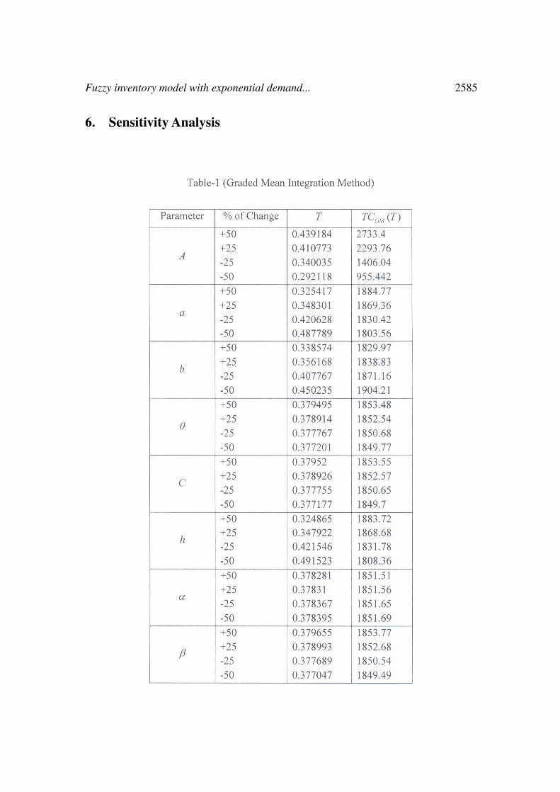
6. Sensitivity Analysis

2586 N.K. Sahoo, et al.

Fuzzy inventory model with exponential demand... 2587
Above figure shows comparison between T V s. Total cost by Graded Mean Integra-tion Method (T C2) and T V s. Total cost by Signed Distance Method (T C3).
We will discuss the effects of the parameters w.r.t. Table 1 and Table 2.
(i) From above we conclude that the optimal cost and time period increases graduallyfor both method when the percentage change in the parameter A.
(ii) When the percentage change in the parameter a and b, the optimal cost slightlyincreases and time period slightly decreases for both method.
(iii) When the percentages change in the parameter θ, α and β the optimal cost and timeperiod changes slightly.
(iv) When the percentage change in the parameter h,the optimal cost increases graduallyand time period decreases gradually for both method.
7. Conclusion
In this paper we have developed a fuzzy inventory model with time-varying demand anddeterioration with salvage value. To capture the real life situation we have considered thatthe major parameters are uncertain and it is possible to describe it by trapezoidal fuzzynumbers. For defuzzification Graded Mean Integration and Signed Distance Method areemployed to evaluate the optimal time period of total cycle length T which minimize thetotal cost.
Numerically we ventured to compare the crisp model with fuzzy model and concludethat if the uncertainties are accounted for in an appropriate manner, the time woulddecrease. Sensitivity analysis is carried out to see how far the output of the model isaffected by changes in its input parameters. The preliminary results indicate that the totalinventory cost increases when we increase the parameters a and b. With the increasedvalue of these parameters, it will subsequently increase the fuzzy cost, but decrease thetime period. Similarly with the decreased value of these parameters it will subsequentlydecrease the fuzzy cost but increase the time period.

2588 N.K. Sahoo, et al.
Here we use different examples to illustrate both the crisp as well as fuzzy modelwhich demonstrate the effect of fuzziness of the parameters on the optimal solution. Incomparison with the crisp model, the fuzzy model is giving the relatively better optimalsolution.
Future suggestions
In the future study it is hoped to incorporate the proposed model into more realisticassumptions, such as probabilistic demand and partial backlogging. The model presentedin this study can be extended in different ways. For instance, the model can be extendedfor non-instantaneous receipt of orders as well as shortages.
References
[1] Bellan, R.E., Zadeh, L.A., Decision-making in a fuzzy environment, Manag. Sci.17(4), 141–164 (1970).
[2] Chang, S.C., Yao, J.S., Lee, H.M., Economic reorder point for fuzzy backorderquantity, European Journal of Operational Research. 109, 183–202 (1998).
[3] Ghare, P.M., Schrader, G.F., A model for exponential decaying inventory, J. Ind.Eng. 14, 238–243 (1963).
[4] Hariga, M.A., Optimal EOQ models for deteriorating items with time-varying de-mand, J. Oper. Res. Soc. 47, 1228–1246 (1996).
[5] Heng, K.J., Labban, J., Linn, R.J., An order-level lot-size inventory model fordeteriorating items with finite replenishment rate. Comp. Ind. Eng. 20, 187–197(1991)
[6] Hollier, R.H., Mak, K.L., Inventory replenishment policies for deteriorating itemsin a declining market, Int. J. Prod. Res. 21, 813–826 (1983).
[7] Hsieh, C.H., Optimization of fuzzy production inventory models. Information Sci-ences. 146, 29–40 (2002).
[8] Jaggi, C.K., Aggarwal, K.K., Goel, S.K., Optimal order policy for deterioratingitems with inflation induced demand, Int. J. Prod. Eccon. 103, 707–714 (2006).
[9] Jaggi, C.K., Pareek, S., Sharma,A., Nidhi, Fuzzy Inventory Model for DeterioratingItems with Time-varying Demand and Shortages, American Journal of OperationalResearch. 2(6), 81–92 (2012).
[10] Kao, C., Hsu, W.K., Lot size-reorder point inventory model with fuzzy demands,Computers and mathematics with applications, 43, 1291–1302 (2002).
[11] Mishra, P., Shah, N.H., Inventory management of time dependent deterioratingitems with salvage value, Applied Mathematical Sciences, 2 (16), 793–798 (2008).
[12] Moon, I., Giri, B.C., Ko, B., Economic order quantity models for ameliorating/deteriorating items under inflation and time discounting, Eur. J. oper. Res., 162,773–785 (2005).
Fuzzy inventory model with exponential demand... 2589
[13] Park, K.S., Fuzzy set theoretic interpretation of economic order quantity, IIIETransactions on Systems, Man and Cybernetics, 17, 1082–1084 (1987).
[14] Sarker, B.R., Mukherjee, S., Balan, C.V., An order-level lot size inventory modelwith inventory-level dependent demand and deterioration, Int. J. Prod. Eco. 48,227–236 (1997).
[15] Vujoservic et al., EOQ formula when inventory cost is fuzzy, Int. J. Prod. Eco. 45,499–504 (1996).
[16] Wee, H., A deterministic lot-size inventory model for deteriorating items with short-ages and a declining market, Comp. Oper. Res. 22, 345–356 (1995).
[17] Yao, J.S., Chiang, J., Inventory without backorder with fuzzy total cost and fuzzystoring cost defuzzified by centroid and signed distance, Eur. J. Oper. Res. 148,401–409 (2003).
[18] Yao, J.S., Lee, H.M., Fuzzy inventory with backorder for fuzzy order quantity,Information Science, 93, 283–319 (1996).
[19] Yao, J.S., Lee, H.M., Fuzzy inventory with or without backorder for fuzzy orderquantity with trapezoidal fuzzy number, Fuzzy sets and Systems, 105, 311–337(1999)
[20] Zadeh, L.A., Fuzzy Sets, Information and Control, 8, 338–353 (1965).
[21] Zadeh, L.A., Outline of a new Approach to the Analysis of Complex Systems andDecision Processes, IEEE Transactions on Systems. Man and Cybernetics, SMC-3,28–44 (1973).