Future Supply of Oil and Gas from the Permian Basin of West Texas and Southeastern New Mexico ·

Future Supply of Oil and Gas from the Permian Basin of West Texas and Southeastern Ne\N Mexico A report of the Interagency Oil and Gas Supply Proiect,

U.S. Department of the Interior and U.S. Department of Energy

GEOLOGICAL SURVEY CIRCULAR 828

1980

United States Department of the Interior CECIL D. ANDRUS, Secretary

Geological Survey H. William Menard, Director

Library of Congress in Publication Data

United States. Interagency Oil and Gas Supply Project. Future supply of oil and gas from the Permian Basin of west

Texas and southeastern New Mexico.

(Geological Survey circular ; 828) Bibliography: p. Supt. of Docs. no.: I 19.4/2:828) 1. Petroleum-Texas. 2. Gas, Natural-Texas. 3. Petro­

leum-New Mexico. 4. Gas, Natural-New Mexico. I. Title. II. Series: United States. Geological Survey. Cir­cular; 828.

QE75.C5 no. 828 [TN872.T4] 557.3s 553.2'8'097648 80-607115

Free on application to Branch of Distribution, U.S. Geological Survey 604 South Pickett Street, Alexandria, VA 22304

PREFACE

In 1975, the U.S. Geological Survey issued its Circular 725, entitled "Geological Estimates of Undiscovered Recoverable Oil and Gas Resources in the United States." Using advanced resource-appraisal techniques, the authors of that document presented new data on these resources. The results were essentially geological, and the economics of oil and gas recovery were not ana­lyzed; instead, the analyses assumed the continuation of price/cost relationships and technological trends that prevailed before 1974. The study was not intended to produce schedules describing future oil and gas supply at different price levels and rates of return. Finally, the study specifically excluded shale oil, tar sands, heavy crude oil, gas from tight sandstone formations not already being pro­duced, and oil and gas below waters that were more than 200 m deep.

Recognizing the need to add more of an economic perspective to the estimates, the Interagency Oil and Gas Supply Project was established in mid-1976 to: evaluate any changes in resource estimates that might result from the post-197 4 price levels; incorporate subsequent geological and geophysical information; prepare basin-level marginal cost schedules reflecting both conventional and "enhanced'' oil and gas recovery; and estimate costs for unconventional oil and gas sources.

The interagency agreement (p. 56) was prepared and signed in early 1977 by the Department of the Interior, which included the Office of Minerals Policy and Research Analysis (OMPRA), the Bureau of Mines (BOM), and U.S. Geological Survey (USGS), as lead agency; the Federal Energy Administration (FEA); the Federal Power Commission (FPC); and the Energy Research and Development Administration (ERDA). Subsequently, the involved offices in the BOM, the FEA, the FPC, and ERDA became part of the Department of Energy.

When the project was sta,:rted, no up-to-date model was available that showed marginal-cost schedules of the full spectrum of possible sources on a disag­gregated basis. Those who prepared such schedules had difficulties in separating oil and gas components and in dealing with inadequate data, and the biases in­troduced into historical data covering price-regulated commodities.

In spite of these difficulties, a rational effort has been made to estimate ultimate recovery and the associated costs. The project studies will contain estimates of ultimate recovery at various costs but will not contain predictions of the time of arrival of the supplies, because timing is determined by industry.

With respect to timing, additional recovery becomes progressively more costly as the size of newly discovered fields diminishes, as they become less accessible geographically, and as recovery requires more advanced technology. For the same reasons, progressively greater effort will be required for a given level of production, regardless of the volume of remaining resources. Ultimately, pro­duction must decline.

Although the areas were not defined in the agreement, the project leaders decided to limit the study to three areas: the Permian Basin (a mature producing area), the Gulf of Mexico offshore area (a partially developed area), and the Baltimore Canyon Basin (a frontier area). This report covers only the research on the Permian Basin.

Ill

CONTENTS Page

Preface ---------------------------------------------------------------------- iii Executive summary ------------------------------------------------------------ 1

Permian Basin history and characteristics ------------------------~-------------- 1 Original oil and gas in place --------------------------------------------------- 1 Future field-size distribution -------------------------------------------------'-- 2 Supply from newly discovered fields -------------------------------------------- 4 Additional supply from existing fields ------------------------------------------- 4 Permian Basin supply- retrospect and prospect ---------------------------------- 6 Comparison with earlier assessments ------------------------------------------- 6

Introduction ------------------------------------------------------------------ 9 Abbreviations and definitions ------------------------------------------------- 9 Resource classification ------------------------------------------------------- 9 Explanatory note----------------------------------------------------------- 10 Sensitivity to prices and costs ------------------------------------------------- 11 The Permian Basin pilot area ------------------------------------------------- 12 Approach and general methodology -------------------------------------------- 12 Undiscovered resource appraisal ---------------------------------------------- 12 Discovery-process model ----------------------------------------------------- 13 Engineering and cost analysis for future fields ----------------------------------- 13 The integrating economic model_______________________________________________ 13 Additional oil from known fields ----------------------------------------------- 13 Indicated and inferred reserves ----------------------------------------------- 13 Enhanced oil and gas recovery ------------------------------------------------ 13 Other occurrences ---------------------------------------------------------- 14

Future production of undiscovered oil and gas from tHe Permian Basin------------------- 14 Permian Basin resource appraisal ---------------------------------------------- 14

Geology --------------------------------------------------------------- 14 Analysis and assessment-------------------------------------------------- 15 Geologic analyses -------------------------------------------------------- 17 Statistical analysis ------------------------------------------------------- 18 Subjective probability procedures ------------------------------------------ 18 Methods for pool-size assessment ------------------------------------------- 18 Summary results-------------------------------------------------------- 19

The discovery-process model -------------------------------------------------- 20 Expressing the data in depth intervals--------------------------------------- 21 Form of the model ------------------------------------------------------- 22 Forecasting future rates of recovery ---------------------------------------- 25 Conclusions ------------------------------------------------------------ 26

Engineering and cost analysis for future fields----------------------------------- 28 Exploration costs -------------------------------------------------------- 29 Field design and investment costs ------------------------------------------ 29 Production schedules and production costs ----------------------------------- 33 Assumptions for present value calculations ----------------------------------- 36

Estimated marginal cost functions for undiscovered recoverable oil and gas resources in the Permian Basin ------------------------------------------------------- 3 7

Methodology ----------------------------------------------------------- 39 Summary of results------------------------------------------------------ 41 Conclusion ------------------------------------------------------------- 44

Additional supplies from known fields ---------------------------------------------- 44 Estimates of indicated and inferred reserves------------------------------------- 44

Indicated reserves ------------------------------------------------------- 46 Inferredreserves________________________________________________________ 46 General outline of data and methods ---------------------------------------- 4 7 Method of analysis ------------------------------------------------------- 48 A variation on the method of analysis ---------------------------------------- 50 Summary -------------------------------------------------------------- 50

v

Page

Enhanced oil and gas recovery---------------------------------------------------- 50 Enhanced oil recovery------------------------------------------------------- 50 ~ethodology_______________________________________________________________ 51

Enhanced gas recovery------------------------------------------------------ 52 Expanded production from known fields: an appraisal of results------------------------- 53 Notes on methodology ----------------------------------------------------------- 54 Interagency agreement for an oil and gas supply project------------------------------- 56 Participants in the project------------------------------------------------------- 57 References cited --------------------------------------------------------------- 58

ILLUSTRATIONS

FIGURE 1. ~ap showing oil and gas fields in the Permian Basin -------------------------------------------------2-6. Graphs showing:

2. Original oil and natural gas in place in the Permian Basin-----------------------------------------3. Undiscovered oil and natural gas in place in the Permian Basin ------------------------------------4. Fuel supply from future discoveries in the Permian Basin----------------------------------------5. Fuel supply from future discoveries in the Permian Basin by commodity----------------------------6. Potential new supplies of oil and gas in the Permian Basin ----------------------------------------

7. Resource classification diagram, total resources ----------------------------------------------------8. Map showing structural elements in the Permian Basin ----------------------------------------------

9-32. Graphs showing: 9. Historic finding rate for oil, 1920-74, Permian Basin--------------------------------------------

10. Historic finding rate for nonassociated natural gas, 1920-7 4, Permian Basin -------------------------11. Probability distribution of the total Paleozoic undiscovered oil in place, aggregated for depths

of0-20,000feet _______________________________________________________________________ _

12. Probability distribution of total Paleozoic undiscovered dissolved and associated gas in place, aggregated fordepthsof0-20,000feet ______________________________________________________________ _

13. Probability distribution of total Paleozoic undiscovered nonassociated gas in place, aggregated for depths of 0-30,000 feet------------------------------------------------------------------------

14. Probability distribution of total Paleozoic undiscovered gas (dissolved, associated, nonassocizted) in place, aggregated for depths of 0-30,000 feet-----------------------------------------------------

15. Lognormal-probability size distribution of undiscovered Permian oil pools in depths of 0-10,000 and 10,000-20,000 feet ---------------------------------------------------------------------

16. Lognormal-probability size distribution of undiscovered Carboniferous oil pools in depths of 0-10,000 and 10,000-20,000 and 10,000-20,000 feet-----------------------------------------------------

17. Lognormal-probability size distribution of undiscovered nonassociated Carboniferous gas po'lls in depths of 0-10,000, 10,000-20,000, and deeper than 20,000 feet---------------------------------------

18. Average depth of exploratory wells as a function of cumulative exploratory wells drilled in the Permian

Basin --------------------------------------------------------------------------------19. Exploratory well drilling and equipping costs as a function of well depth in the Permian Basin in 1975 ___ _ 20. Total exploration cost per exploratory well (minus cost of acquiring undeveloped acreage) as a function of

drilling cost per well in 1977 --------------------------------------------------------------21. Drilling and equipping cost per development well versus depth in the Permian Basin in 1975------------22. Cost of development of dry hole versus depth in the Permian Basin in 1975 --------------------------23. Lease equipment cost per well versus depth for primary oil production in the Permian Basin in 1976 ____ _ 24. Oil-production-decline curves for primary recovery at 7,200 feet in the Permian Basin-----------------25. Percent of expected ultimate gas recovery as a function of percent of expected ultimate oil recovery in the

Permian Basin -------------------------------------------------------------------------26. Nonassociated gas-well-production curve for a class 13 field in the depth bracket of 0-5,000 feet in the

Permian Basin ------------------.... ------------------------------------------------------27. Annual direct operating cost per producing oil well versus depth for primary recovery in th~ Permian

Basin in 1976-------------------.... ------------------------------------------------------28. Annual direct operating cost per producing oil well versus depth for secondary recovery in the Permian

Basin in 1976--------------------------------------------------------------------------29. Exploratory wells projected to be drilled in the Permian Basin as a function of price of oil anct gas and rate

ofreturnoninvestment ________________________________________________________________ _

30. Marginal cost of recoverable oil and gas resources from undiscovered deposits in the Permian Basin- 5 percent discounted cash-flow rate of return-------------------------------------------------

31. Marginal cost of recoverable oil and gas resources from undiscovered deposits in the Permian Basin -15 percent discounted cash-flow rate of return-------------------------------------------------

32. Marginal cost of recoverable oil and gas resources from undiscovered deposits in the Permian Basin- 25 .Percent discounted cash-flow rate of return -------------------------------------------------

VI

Page

3 4 6 7 8

10 16

18 19

21

22

23

24

25

25

26

29 30

31 34 36 37 38

39

40

41

42

44

45

46

47

Page

FIGURE 33. Diagram of production, reserves, and residual oil in place in the Permian Basin, exclusive of "Spraberry'' TT~end, December 31, 1977 ------------------------------------------------------------------------ 51

34. Map showing areas of the Permian Basin for enhanced gas recovery------------------------------------ 53

TABLES

Page

TABLE 1. Future exploration drilling and supply from undiscovered recoverable oil and gas resources in the Permir'l

Basin ----------------------------------------------------------------------------------- 5 2. Potential for enhanced recovery in the Permian Basin ----------------------------------------------- 5 3. Potential new recoverable supplies of oil and gas from the Permian Basin-------------------------------- 7 4. Discovered oil and gas in place, Permian Basin (1921-December 31, 1974) ------------------------------- 15

5-7. Estimates of: 5. Total undiscovered hydrocarbons in place ----------------------------------------------------- 20 6. Undiscovered hydrocarbons in place by depth interval___________________________________________ 20 7. Mean depths of occurrence of undiscovered hydrocarbons in place-all Paleozoic systems --------------- 20

8. Field-size classes ----------------------------------------------------------------------------- 22 9. Comparison of the numbers of discoveries through 1974 with the number forecast, keyed on the pre-1961 dis-

covery and exploratory drilling data in the 0-5,000-foot depth interval--------------------------·---- 24 10-13. Expected ultimate number of fields remaining to be discovered after 1974:

10. In the 0-5,000-foot depth interval___________________________________________________________ 27 11. In the 5,000-10,000-foot depth interval_______________________________________________________ 27 12. In the 10,000-15,000-foot depth interval______________________________________________________ 27 13. In the 15,000-20,000-foot depth interval ------------------------------------------------------ 28

14. Number of discoveries expected to be made in each size class with the first increment of 1,000 exploratory holes drilled in the Permian Basin after 1974-------------------------------------------------------- 28

15. Ratio of oil fields to total fields in the Permian Basin------------------------------------------------- 30 16. Expected ultimate oil recovery per field in the Permian Basin----------------------------------------- 30 17. Expected ultimate oil recovery per well from primary oil fields in the Permian Basin----------------------- 31 18. Expected ultimate associated-dissolved gas recovery per oil well from primary fields in the Permian Basin_____ 31 19. Expected ultimate oil recovery per well from secondary and pressure maintenance fields in the Permian Basin_ 32 20. Expected ultimate gas recovery per oil well from secondary and pressure maintenance fields in the Permb.n

Basin ----------------------------------------------------------------------------------- 32 21. Expected ultimate nonassociated gas recovery per field in the Permian Basin---------------------------- 32 22. Expected ultimate nonassociated gas recovery per well in the Permian Basin----------------------------- 32 23. Ratio of primary oil fields to total oil fields in the Permian Basin --------------------------------------- 32 24. Cost of lease equipment per nonassociated gas development well in the Permian Basin in 1977 dollars--------- 33 25. Exponential oil-well decline rates per year in the Permian Basin-------------------------------------- 34 26. Annual direct operating expenses for nonassociated gas wells in the Permian Basin in 1977 dollars----------- 36 27. Potential recoverable oil and gas resources from future discoveries in the Permian Basin as a function of output

price, marginal finding cost, marginal production cost, exploratory wells, and return on investment _______ 43 28. Growth in estimates of original oil in place for the Permian Basin -------------------------------------- 48 29. Growth in estimates of recoverable natural gas for the Permian Basin---------------------------------- 49 30. Classification of sample reservoirs selected for enhanced oil recovery in the Permian Basin----------------- 52 31. Enhanced oil recovery potential of the Permian Basin------------------------------------------------ 52 32. Enhanced gas recovery potential of the Permian Basin----------------------------------------------- 53

vii

FUTURE SUPPLY OF OIL AND GAS FROM THE PERMIAN BASIN OF WEST TEXAS AND SOUTHEASTERN NEW MEXICO

A REPORT OF THE INTERAGENCY OIL AND GAS SUPPLY PROJECT,

U.S. DEPARTMENT OF THE INTERIOR AND U.S. DEPARTMENT OF ENERGY

EXECUTIVE SUMMARY

In mid-1976, the Interagency Oil and Gas Supply Project was established, by agreement among several Federal agencies to estimate how much oil and gas might be made available in the future at various price levels from all potential sources in the United States. The scope of investigation includes supplies of oil and gas from presently known fields through additional drilling and enhanced-recovery methods, from fields not yet discovered, and from a variety of sources categorized as "unconventional" (such as oil shale, tar sands, and gas from coal beds and geopressured brines). Liquid and gaseous fuels synthesized from coal or other substances are not considered.

The project, with the U.S. Geological Survey as lead agency, is designed to extend the analysis described in U.S. Geological Survey Circular 725 (Miller and others, 1975) by incorporating new geological and geophysical data, by supplying an economic perspective, and by addressing the outlook for enhanced recovery and unconventional sources not treated in the earlier study. As a prelude to a nationwide assessment, three areas were selected for study on a test basis: the Permian Basin of west Texas and southeastern New Mexico (a mature producing area), the Gulf of Mexico offshore (a partly developed basin), and the Baltimore Canyon Basin of the Atlantic Outer Continental Shelf (a frontier area). This report analyzes the oil and gas pros­pects of the Permian Basin. The basin is shown in figure 1 in relation to western Texas and eastern New Mexico, Region 5 in Circular 725. The Permian Basin covers roughly 50 percent of the 173,000 square-mile total area of Region 5.

The report begins with a survey of known resources of oil and gas in the Permian Basin1 from which an estimate is made of the tptal amount of oil and gas discovered by the end of December 1974. Next, estimates are made of the amounts of undiscovered oil and gas thought to exist at various levels of probability; these data include the number of reservoirs estimated to exist in each of 20 size classes and in three successive depth intervals of 10,000 feet each. After this appraisal of the basin's original en­dowment of oil and gas, both discovered and undiscovered, a projection is made of the most likely sequence in which the un­discovered reservoirs may be found and the amount of ex­ploratory drilling that will be required to find them. Explora­tion, development, and production costs are then introduced and are used to obtain estimates of the volumes of undiscovered oil and gas that will actually be found and produced at different assumed price levels and rates of return.

In addition to supply from new discoveries, relatively large amounts of oil and gas are expected to be produced from presently known fields, either through drilling that extends field limits or penetrates new pools within the field, or from new technologies that enable recovery of a greater fraction of the original oil or gas in the field than that which can now be

1 The Permian Basin corresponds closely, but not exactly, to the area designated by the Texas Railroad Commission as Districts 7C, 8, and 8A, plus that designated as southeast New Mexico by the American Petroleum Institute and the American Gas Association. As a matter of convenience in this report, it is considered identical with these districts, unless otherwise specified.

1

recovered through conventional techniques. The volume of hydrocarbons obtained from such enhanced-recovery measures is estimated for different price levels and rates of re';urn in the same manner that volumes of undiscovered oil ard gas are estimated.

PERMIAN BASIN HISTORY AND CHARACTE.RISTICS

The Permian Basin is a mature petroleum-producing province extending over about 80,000 square miles of west Texas and southeastern New Mexico; its sedimentary rocks are more than 25,000 feet thick in its deepest parts. The basin is chrracterized by arches, platforms, basins, and shelves formed during the later Paleozoic periods; the Midland, Delaware, and Val Verde Basins and the Central Basin Platform are of particular in­terest.

The Permian Basin has been a prolific source of petroleum hydrocarbons since the initial discoveries were made in 1921. Production to the end of 1976 amounted to 18.6 billior barrels of crude oil and 55.8 trillion cubic feet of natural gas; 5.5 billion barrels and 18.2 trillion cubic feet remained as proved reserves on that date. Virtually all the petroleum was found ir Paleozoic sediments, most (71 percent) of the oil being in the relatively shallow Permian rocks and most of the nonassociated gas, in deeper strata of Devonian age and older. Oil has been produced from wells that are deeper than 14,000 feet, and ga~ has been produced from depths of more than 21,000 feet. Although car­bonate reservoirs predominate in this province, large quantities of both oil and gas have been found in sandstone formations. Distribution of hydrocarbons is roughly equal in structural and in stratigraphic traps.

The oil and gas resources of the Permian Basin are for all practical purposes confined to those occurring as co"1ventional accumulations, including those amounts requirir~ special recovery techniques to produce. Present data indicate that lit­tle, if any, oil and gas are available from oil shale, brown or black shale, rich in organic matter, tar sand, asphalt, heavy oil, and no methane is available in brines or hydrates; no supply from such sources is expected in the foreseeable future.

ORIGINAL OIL AND GAS IN PLACE

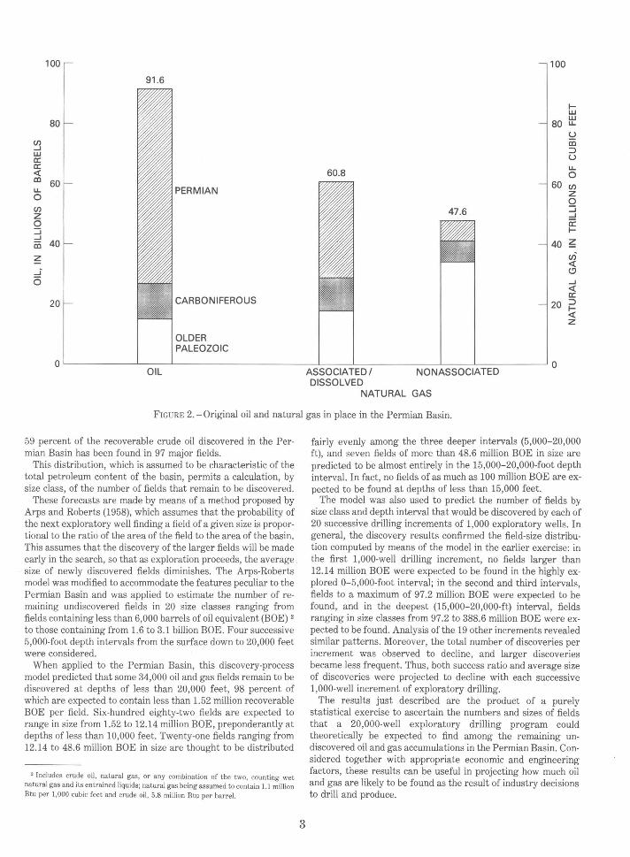
Discovered deposits as of December 31, 1974, were estimated to be 92 billion barrels of oil and 108 trillion cubic feet of natural gas, distributed as shown in figure 2. Of these volumef',. about 26 percent of the oil and 75 percent of the gas are expected to be recovered under present economics and technology. Although these percentages may increase somewhat as anticipated im­provements in recovery techniques are made, most of the oil and some of the gas will always be too difficult or too costly to produce and cannot be considered recoverable resources.

The amount of oil and gas remaining to be discovered in the Permian Basin has been appraised on the basis of (1) an inten­sive review of basin geology, (2) a statistical analysis of discovery experience, and (3) the application of professional judgment to obtain estimates of oil and gas in place at each of various levels of probability (95, 75, 25, and 5 perce:-1t), plus a

101° 100° ggo 98~

50 100 MILES

0 50 100 KILOMETERS -lfiJ Oil/gas field ~ Study area -.-- Boundary, USGS Region 5

FIGURE 1. -Oil and gas fields in the Permian Basin.

modal estimate and a calculated statistical mean for each of three successive depth intervals of 10,000 feet. These estimates were then aggregated by means of Monte Carlo techniques into totals for the basin by depth interval. The mean values for each depth interval, plus the values estimated for the 95- and 5-percent probability levels are shown graphically in figure 3. A comparison of the mean values of undiscovered oil and gas with the discovered amounts (see fig. 2) suggests that almost 95 per­cent of the oil and 83 percent of the gas originally contained in the Permian Basin may already have been found.

2

FUTURE FIELD-SIZE DISTRIBUTION

The Permian Basin has long been the focm of an intensive search, which has resulted in the discovery of 4,036 oil and gas fields by 30,340 exploratory wells drilled from 1921 through 1974. The province shows a typical distribution pattern of fields by size and number. A very few very large fields are at one end of a spectrum that trends toward successively greater numbers of smaller and smaller fields, so that most of the basin's oil and gas is concentrated in a relatively few large fie1ris. For example,

100 100

91.6

I-w

80 w

80 u..

~ (/) CD ....J :::> w u a: a: u.. <t 60.8 0 CD 60 60

PERMIAN (/) u.. z 0 0

(/) 47.6 ::::i z ....J

0 a: ::::i I-::::! 40 40 ~ CD

z u) <t

....J- (.!)

0 ....J <t

CARBONIFEROUS a:

20 20 :::> I-<t z

OLDER PALEOZOIC

0 0 OIL ASSOCIATED I NONASSOCIATED

DISSOLVED NATURAL GAS

FIGURE 2.-0riginal oil and natural gas in place in the Permian Basin.

59 percent of the recoverable crude oil discovered in the Per­mian Basin has been found in 97 major fields.

This distribution, which is assumed to be characteristic of the total petroleum content of the basin, permits a calculation, by size class, of the number of fields that remain to be discovered.

These forecasts are made by means of a method proposed by Arps and Roberts (1958), which assumes that the probability of the next exploratory well finding a field of a given size is propor­tional to the ratio of the area of the field to the area of the basin. This assumes that the discovery of the larger fields will be made early in the search, so that as exploration proceeds, the average size of newly discovered fields diminishes. The Arps-Roberts model was modified to accommodate the features peculiar to the Permian Basin and was applied to estimate the number of re­maining undiscovered fields in 20 size classes ranging from fields containing less than 6,000 barrels of oil equivalent (BOE) 2

to those containing from 1.6 to 3.1 billion BOE. Four successive 5,000-foot depth intervals from the surface down to 20,000 feet were considered.

When applied to the Permian Basin, this discovery-process model predicted that some 34,000 oil and gas fields remain to be discovered at depths of less than 20,000 feet, 98 percent of which are expected to cont<tin less than 1.52 million recoverable BOE per field. Six-hundred eighty-two fields are expected to range in size from 1.52 to 12.14 million BOE, preponderantly at depths of less than 10,000 feet. Twenty-one fields ranging from 12.14 to 48.6 million BOE in size are thought to be distributed

2 Includes crude oil, natural gas, or any combination of the two, counting wet natural gas and its entrained liquids; natural gas being assumed to contain 1.1 million Btu per l ,000 cubic feet and crude oil, 5.8 million Btu per barrel.

3

fairly evenly among the three deeper intervals (5,000-20,000 ft), and seven fields of more than 48.6 million BOE in size are predicted to be almost entirely in the 15,000- 20,000-foot depth interval. In fact, no fields of as much as 100 million BOE are ex­pected to be found at depths of less than 15,000 feet.

The model was also used to predict the number of fields by size class and depth interval that would be discovered by each of 20 successive drilling increments of 1,000 exploratory wells. In general, the discovery results confirmed the field-size distribu­tion computed by means of the model in the earlier exercise: in the first 1,000-well drilling increment, no fields larger than 12.14 million BOE were expected to be found in the highly ex­plored 0-5,000-foot interval; in the second and third intervals, fields to a maximum of 97.2 million BOE were expected to be found, and in the deepest (15,000-20,000-ft) interval, fields ranging in size classes from 97.2 to 388.6 million BOE were ex­pected to be found. Analysis of the 19 other increments revealed similar patterns. Moreover, the total number of discoveries per increment was observed to decline, and larger discoveries became less frequent. Thus, both success ratio and average size of discoveries were projected to decline with each successive 1,000-well increment of exploratory drilling.

The results just described are the product of a purely statistical exercise to ascertain the numbers and sizes of fields that a 20,000-well exploratory drilling program could theoretically be expected to find among the remaining un­discovered oil and gas accumulations in the Permian Basin. Con­sidered together with appropriate economic and engineering factors, these results can be useful in projecting how much oil and gas are likely to be found as the result of industry decisions to drill and produce.

OIL

10

5%

(/) EXPLANATION ...J

NATURAL GAS

ASSOCIATED AND

DISSOLVED

NONASSOCIATED 25

20

1-w

15 w u.

~ al ::J u w 5%, 95%=Volumes estimated at 5 percent a: z a: M

and 95 percent probability M 0 <( M Statistical mean value ::::i al 5 10 ...J

z a: 0 1-::::i ...J

al 5%

5

0 CHO 1Q-20

DEPTH, IN THOUSANDS OF FEET DEPTH, IN THOUSANDS OF FEET FIGURE 3.- Undiscovered oil and natural gas in place in the Permian Basin.

SUPPLY FROM NEWLY DISCOVERED FIELDS

Translating estimates of undiscovered oil and gas into pro­ducible reserves requires the introduction of economic con­siderations that determine whether the capital needed to bring those resources to market will, in fact, be invested. In the study, this was done in two steps. In the first step, field development and production costs were estimated. Then, in the second step, a discounted cash-flow analysis was used to estimate the amounts of undiscovered oil and gas that the oil industry would find and produce at different market prices and rates of return that were based on development and production costs. The results of the analysis are summarized in table 1 in terms of exploratory wells drilled and economically producible hydrocarbons discovered at each price level and rate of return.

The data presented in the tables indicate the mature stage of exploration in the Permian Basin and the response of supply, both to exploration effort and to price. The 30,000 exploratory wells projected to be drilled at $40 per BOE under a 25 percent rate of return are predicted to result in the discovery of 3.85 billion BOE, an amount approximately one-tenth of the volume of oil and gas found by the first 30,000 exploratory holes drilled in the basin. Table 1 also shows that, at all rates of return, discovery response to price diminishes sharply at prices greater than $25 per BOE. For example, in figure 4, which shows discoveries at a 15 percent rate of return, the first $15 incre­ment above the base of $10 elicits a 185-percent increase in sup­ply; the second increment of $15 yields an increase of less than 25 percent.

4

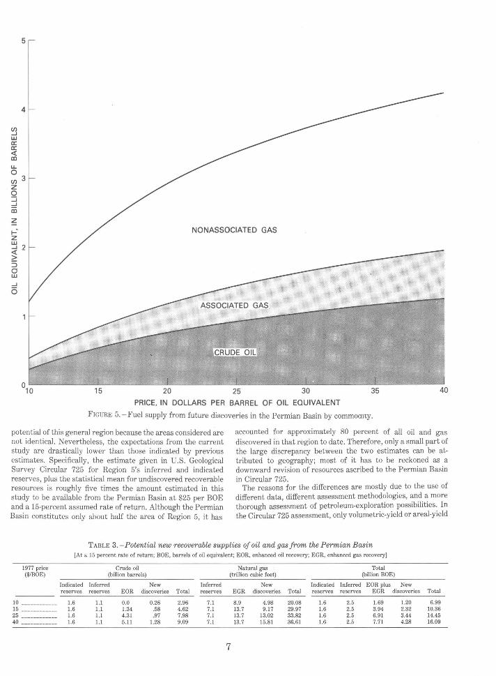
Another notable feature is the preponderance of natural gas, which constitutes approximately two-thirds of the energy value of the hydrocarbons projected to be discovered (see fig. 5). This distribution is almost the reverse of that shown by discovery ex­perience through 1974, when crude oil constituted two-thirds of the total hydrocarbons found.

ADDITIONAL SUPPLY FROM EXISTING FIELDS

In addition to the oil and gas from future discoveries, substan­tial amounts of both are expected to be produced from already discovered fields, in addition to the amounts presently estimated to be recoverable. These "bonus" amounts result from (1) tlw fact that the larger oil and gas fields routinely "grow" from year to year as field limits are extended by drilling, new pools are found within fields, and additinal information about the field permits the upward revision of previous estimates; 3

and (2) technological improvements in recovery operations that permit a larger fraction of the total resources in the ground to be produced than that previously expected.

The fact has long been accepted that many fields are actually bigger than estimates have indicated. Accounting for proved reserves-oil and gas that can definitely be produced from a field on the basis of existing economics and technology- is necessarily conservative and includes only resources under acreage that can be drained by existing wells and in the

3 However, such additional data may also result in a downward revision of previous estimates.

TABLE 1.-Future exploration drilling and supply from undis­covered recoverable oil and gas resources in the Permian Basin

[BOE, barrels of oil equivalent]

Output Wells Wells Wells price drilled BOE drilled BOE drilled BOE

($/BOE) (thou- (billions) (thou- (billions) (thou- (billions) sands) sands) sands)

5 percent rate of 15 percent rate of 25 percent rate of return return return

10 ------------ 10 2.04 5 1.20 2 0.54 15 ------------ 19 3.03 12 2.32 8 1.77 20 ------------ 26 3.57 18 2.95 12 2.33 25 ------------ 33 4.00 24 3.44 17 2.87 30 ------------ 38 4.27 29 3.77 22 3.30 35 ------------ 43 4.50 34 4.08 26 3.60 40 ------------ 48 4.71 38 4.28 30 3.85

immediately adjoining undrilled parts that are judged to be pro­ductive on the basis of geologic and engineering data. In 1966, for example, the American Petroleum Institute (1967) estimated that the total amount of oil that might be recovered from all fields discovered by that date was 112 billion barrels. By 1976, the estimate for these fields had been raised to 129 billion barrels- a "growth" of 17 billion barrels that resulted chiefly from field extension and development over the interven­ing decade.

This "growth" phenomenon has resulted in efforts to predict the amounts of oil and gas that eventually may be found and produced from existing fields, beyond the proved reserves credited to them at any given date. These incremental amounts of oil and gas that are expected to become proved reserves at some future time are categorized as being either "indicated" or "inferred" reserves, depending largely upon the means by which they are expected to be converted into proved reserves.

Indicated reserves are those volumes of oil that are expected to be economically recoverable by means of improved conven­tional recovery techniques, such as fluid injection, where (1) an improved technique has been installed but its effect cannot yet be fully evaluated, or (2) an improved technique has not been in­stalled but enough is known about its probably success to justify estimates of the volume of oil that might be made available by such means. According to the American Petroleum Institute (American Gas Associates and others, 1977, table 1), these "in-· dicated additional" reserves in the four districts approximating the Permian Basin amounted to 1.6 billion barrels of recoverable crude oil as of December 31, 1976.

Inferred reserves are those that accrue through additional drilling and upward revisions of previous estimates justified by additional knowledge about existing fields. The process for estimating inferred reserves is more reliable for large areas such as the United States as a whole than for smaller, specific regions such as the Permian Basin. Nevertheless, estimates for inferred reserves, which were based on two separate ap­proaches, suggest that an additional 7.1 trillion cubic feet of recoverable gas (1.35 billion BOE) and an additional 4.9 billion barrels of crude oil in place exist as inferred reserves in the Per­mian Basin. At the current recovery rate of 26 percent, an addi­tional 1.3 billion barrels of recoverable oil may be derived from this source. This means that 2.65 billion BOE of petroleum hydrocarbons, which include the gas reserves, are estimated to exist as inferred reserves in the Permian Basin.

Enhanced recovery (that is, recovery techniques going beyond the conventional methods now in use) represents the other ma­jor opportunity for additional supply from existing fields. Enhanced Oil Recovery (EOR) has already resulted in some 300 million barrels that have been produced or proven in a few large

5

reservoirs in the Permian Basin (such as the Scurry Area Canyon Reef Operators Committee (SACROC) carbon dioxide project in the Kelly-Snyder field). If, for example, the an­ticipated recoverable fraction of the Permian Basin's 92 billion barrels of original oil in place could be increased from the cur­rent average of 26 percent to 31 percent, an additional 4.6 billion barrels of oil would become available. Production of this oil will be neither easy nor cheap because many institutional, technical, and economic difficulties bar the way. Still, the oil is known to exist, most of the infrastructure needed to bring it to market is already in place, and sizeable commitments have been made by both the public and the private sectors toward the goal of moving it into the proved reserves category.

This study assumes that satisfactory solutions will eventually be found for the problems that presently beset the prospects for EOR. Estimates, therefore, were made of the amounts of oil that might become available, mainly through carbon dioxide flooding, at different price levels and rates of return, from 96 major reservoirs thought to be technically and economically amenable to EOR techniques. The results were extrapolated to obtain values for the total basin and are presented in table 2. For both the 15- and 25-percent rates of the return, supply response to price diminishes sharply when prices are more than $25 a barrel.

TABLE 2.-Potential for enhanced recovery in the Permian Basin

1977 price t$180E)

10---------------15---------------20 ---------------25 ---------------30 ---------------35 ---------------40 ---------------

[BOE, barrels of oil equivalent]

Oil Gas (billion barrels) (trillion cubic feet)

15 percent 25 percent 15 percent 25 percent rate of rate of rate of rate of return return return return

0.0 0.0 8.9 7.4 1.43 0.20 13.7 13.7 2.93 1.30 13.7 13.7 4.31 2.58 13.7 13.7 4.70 3.65 13.7 13.7 5.08 4.11 13.7 13.7 5.11 4.56 13.7 13.7

The prospects for enhanced gas recovery (EGR) offer the possibility for a significant contribution to future gas supply from the Permian Basin. The target is previously discovered nonassociated gas accumulations in rocks of low permeability that have thus far defied economic production by traditional methods. Rising gas prices and recent improvements in produc­tion technology may provide the means to convert part of these known but presently subeconomic resources into proved reserves.

The geographic focus for EGR in the Permian Basin is in its southeastern corner in three Texas counties. Within this area lie known gas accumulations that can be considered candidates for massive hydraulic fracturing (MHF), in which pressure is as much as 10 times greater than that used in conventional hydraulic fracturing that has long been used to introduce cracks in reservoir rock to facilitate the flow of oil and gas to the well bore.

Data were analyzed to ascertain the amounts of gas that these prospective gas fields might be expected to yield under MHF at two rates of return and several price levels (see table 2). The ex­ercise shows that at a price of $15 or more per BOE, as much as 13.7 trillion cubic feet of gas might become available under cur­rently available MHF technology.

5.-

.. ~ w 0 m

41-

r! (/) ....J w a: a: <( m u.. 0 (/) 31-z 0 w ::::i 0 ....J m m

r! z t-=" z w

21-....J N <( N ~

::J 0 w ....J

6

n-

I I I I I J OL_----------L_--------~----------~~--------~30~--------~35~--------~40 10 15 20 25

PRICE, IN DOLLARS PER BARREL OF OIL EQUIVALENT

FIGURE 4. - Fuel supply from future discoveries in the Permian Basin.

PERMIAN BASIN SUPPLY-RETROSPECT AND PROSPECT

As the result of 6 decades of exploration and development, 24 billion barrels of recoverable crude oil and 7 4 trillion cubic feet of recoverable natural gas had been found in the Permian Basin as of December 31, 1974. By comparison, the analysis of data from this project indicates a potential future supply of 3 billion to 9 billion barrels of crude oil and 20 trillion to 37 trillion cubic feet of natural gas from all sources, a 15-percent rate of return and at a price range of $10 to $40 per BOE. At a 5-percent rate of return, these amounts would be somewhat higher, and at a 25-percent rate, somewhat lower. Supply responsiveness falls off quickly when prices are more than $25 per BOE for both oil and gas. Table 3 recapitulates the supply of oil and gas available from each source at prices of $10, $15, $25, and $40 per BOE at a 15-percent rate of return. Figure 6 represents these values graphically.

The prospect for additional oil from new discoveries is limited. Even at $40 a barrel, no more than 1.3 billion barrels is pro­jected-about 17 percent of the amount expected to be

6

recovered from existing fields and barely 5 percent of the 24 billion barrels discovered previously. By far, the greater part of future oil supply from the Permian Basin is expected to co~e from already discovered fields, primarily from indicated and ~~­ferred reserves at the lower price ranges, and from enhanced 01! recovery at prices of $25 or more per BOE.

The outlook for new discoveries of natural gas is better than that for oil at all price levels, mainly because of the greater · probabilities of finding large accumulations in those stra~ where gas is likely to be found, that is, below 15,000 feet m depth. Even so, however, new discoveries are expected to ac­count for less than half the future supply of gas from the Per­mian Basin. Slightly more than 7 trillion cubic feet is expected from inferred reserves, and as much as almost 14 trillion cubic feet is optimistically projected from enhanced-gas-recovery projects in the tight sands of the basin at prices of $15 and more per BOE.

COMPARISON WITH EARLIER ASSESSMENTS

The results of the Permian Basin study cannot be directly compared with those of other assessments of the petroleum

ll'l CXl c)

5

4

(/) ...J w a: a: <( [II

u. 0 (/) 3 z 0 ::::i ...J

[II

z f-. NONASSOCIATED GAS z w

2 ...J <( ~ ::::> 0 w ...J

0

15 20 25 30 35 40

PRICE, IN DOLLARS PER BARREL OF OIL EQUIVALENT

FIGURE 5.-Fuel supply from future discoveries in the Permian Basin by commomty.

potential of this general region because the areas considered are not identical. Nevertheless, the expectations from the current study are drastically lower than those indicated by previous estimates. Specifically, the estimate given in U.S. Geological Survey Circular 725 for Region 5's inferred and indicated reserves, plus the statistical mean for undiscovered recoverable resources is roughly five times the amount estimated in this study to be available from the Permian Basin at $25 per BOE and a 15-percent assumed rate of return. Although the Permian Basin constitutes only about half the area of Region 5, it has

accounted for approximately 80 percent of all oil and gas discovered in that region to date. Therefore, only a small part of the large discrepancy between the two estimates can be at­tributed to geography; most of it has to be reckoned as a downward revision of resources ascribed to the Permian Basin in Circular 725.

The reasons for the differences are mostly due to the use of different data, different assessment methodologies, and a more thorough assessment of petroleum-exploration possibilities. In the Circular 725 assessment, only volumetric-yield or areal-yield

TABLE 3. - Potential new recoverable supplies of oil and gas from the Permian Basin

1977 price ($/BOE)

10 ------------15 ------------25 ------------40 -------- ----

[At a 15 percent rate of return; BOE, barrels of oil equivalent; EOR, enhanced oil recovery; EGR, enhanced gas recovery]

Crude oil Natural gas Total (billion barrels) (trillion cubic feet) (billion BOE)

Indicated Inferred New Inferred New Indicated Inferred EOR plus New reserves reserves EOR discoveries Total reserves EGR discoveries Total reserves reserves EGR discoveries

1.6 1.1 0.0 0.26 2.96 7.1 8.9 4.98 20.08 1.6 2.5 1.69 1.20 1.6 1.1 1.34 .58 4.62 7.1 13.7 9.17 29.97 1.6 2.5 3.94 2.32 1.6 1.1 4.31 .97 7.98 7.1 13.7 13.02 33.82 1.6 2.5 6.91 3.44 1.6 1.1 5.11 1.28 9.09 7.1 13.7 15.81 36.61 1.6 2.5 7.71 4.28

7

Total

6.99 10.36 14.45 16.09

25

20

(/)

u:l 15 a: a: <X: CD

z 0 ::J g 10

5

75

1-UJ UJ 50 LL

~ CD ::> u z Q _J 25 _J

a: 1-

CRUDE OIL

NATURAL GAS

NEW DISCOVERIES

ENHANCED OIL RECOVERY

O ___.____._~P_A_S_T--'-'-'-----'"' 1 0

PRODUCTION FUTURE SUPPLY BASED ON PRICE PER BARREL AND PROVED OF OIL EQUIVALENT (1977 DOLLARS)

RESERVES 1921-74

FIGUI{E 6.- Potential new supplies of oil and gas in the Permian Basin

8

analytical techniques were used. In the more recent assessment made here, a comprehensive field and pool data file was used, and abundant drilling and finding-rate studies were conducted along with a thorough review of the geology by stratigraphic units. The net result was a sharper perspective on the petroleum potential of this mature province and, possibly, a inore reliable estimate. As has been illustrated by the differences between this study and Circular 725, reassessments can be expected to change over time as significant new data are acquired and new methods are used. These innovations, however, will not necessarily result in decreased assessments. Accordingly, to extrapolate a reduced expectation nationwide from the reduced assessment of the Permian Basin is not ap­propriate. The planned future assessments for other areas may be more optimistic than those offered previously as a result of new information or the application of different methodologies.

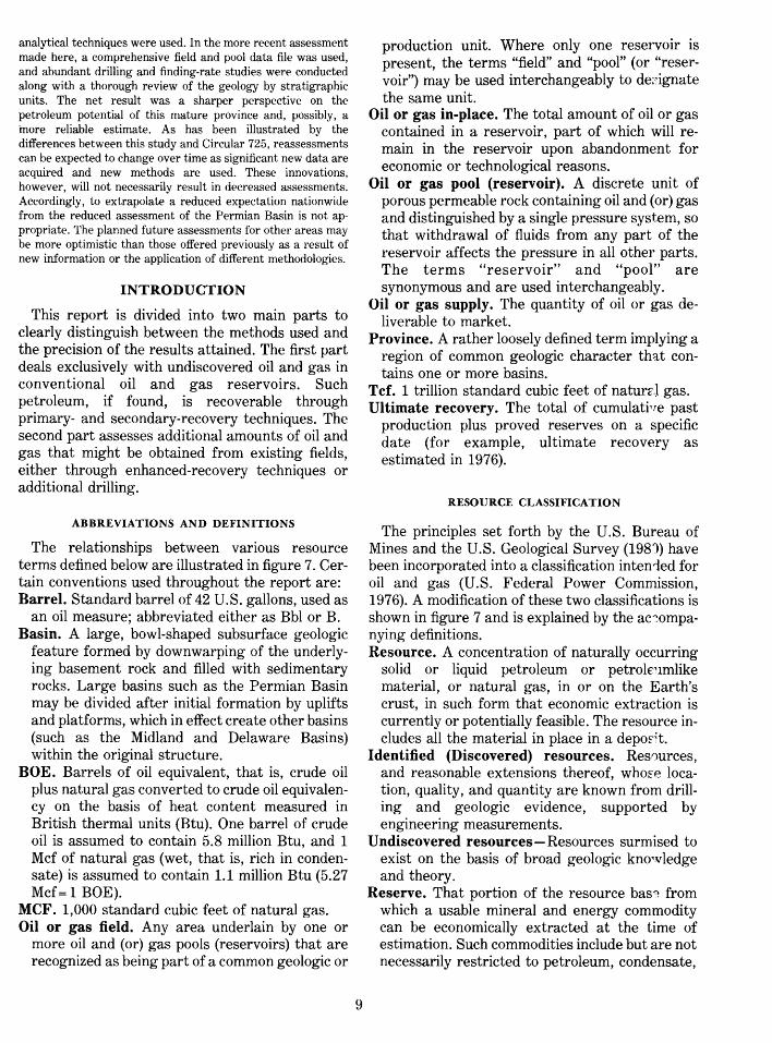
INTRODUCTION

This report is divided into two main parts to clearly distinguish between the methods used and the precision of the results attained. The first part deals exclusively with undiscovered oil and gas in conventional oil and gas reservoirs. Such petroleum, if found, is recoverable through primary- and secondary-recovery techniques. The second part assesses additional amounts of oil and gas that might be obtained from existing fields, either through enhanced-recovery techniques or additional drilling.

ABBREVIATIONS AND DEFINITIONS

The relationships between various resource terms defined below are illustrated in figure 7. Cer­tain conventions used throughout the report are: Barrel. Standard barrel of 42 U.S. gallons, used as

an oil measure; abbreviated either as Bbl or B. Basin. A large, bowl-shaped subsurface geologic

feature formed by downwarping of the underly­ing basement rock and filled with sedimentary rocks. Large basins such as the Permian Basin may be divided after initial formation by uplifts and platforms, which in effect create other basins (such as the Midland and Delaware Basins) within the original structure.

BOE. Barrels of oil equivalent, that is, crude oil plus natural gas converted to crude oil equivalen­cy on the basis of heat content measured in British thermal units (Btu). One barrel of crude oil is assumed to contain 5.8 million Btu, and 1 Mcf of natural gas (wet, that is, rich in conden­sate) is assumed to contain 1.1 million Btu (5.27 Mcf= 1 BOE).

MCF. 1,000 standard cubic feet of natural gas. Oil or gas field. Any area underlain by one or

more oil and (or) gas pools (reservoirs) that are recognized as being part of a common geologic or

9

production unit. Where only one reservoir is present, the terms "field" and "pool" (or "reser­voir") may be used interchangeably to de;;:ignate the same unit.

Oil or gas in-place. The total amount of oil or gas contained in a reservoir, part of which will re­main in the reservoir upon abandonment for economic or technological reasons.

Oil or gas pool (reservoir). A discrete unit of porous permeable rock containing oil and (or) gas and distinguished by a single pressure system, so that withdrawal of fluids from any part of the reservoir affects the pressure in all other parts. The terms "reservoir" and "pool" are synonymous and are used interchangeably.

Oil or gas supply. The quantity of oil or gas de­liverable to market.

Province. A rather loosely defined term implying a region of common geologic character th::tt con­tains one or more basins.

Tcf. 1 trillion standard cubic feet of naturd gas. Ultimate recovery. The total of cumulati1re past

production plus proved reserves on a specific date (for example, ultimate recovery as estimated in 1976).

RESOURCE CLASSIFICATION

The principles set forth by the U.S. Bureau of Mines and the U.S. Geological Survey (1981) have been incorporated into a classification inten1ed for oil and gas (U.S. Federal Power Commission, 1976). A modification of these two classifications is shown in figure 7 and is explained by the ac~ompa­nying definitions. Resource. A concentration of naturally occurring

solid or liquid petroleum or petrolenmlike material, or natural gas, in or on the Earth's crust, in such form that economic extraction is currently or potentially feasible. The resource in­cludes all the material in place in a depofit.

Identified (Discovered) resources. Resr)urces, and reasonable extensions thereof, whoFe loca­tion, quality, and quantity are known from drill­ing and geologic evidence, supported by engineering measurements.

Undiscovered resources- Resources surmised to exist on the basis of broad geologic knowledge and theory.

Reserve. That portion of the resource bas~ from which a usable mineral and energy commodity can be economically extracted at the time of estimation. Such commodities include but are not necessarily restricted to petroleum, condensate,

~ ~ 0 z 0 u UJ

u .~ coo

=>z UlQ

u UJ

U) UJ u

c:Z UJUJ IC: 1--C: 0::::>

u u 0

DISCOVERED UNDISCOVERED

PROVED IINDICATEDIINFERRED

RESERVES

-

RESOURCES

J I I I I T

I I I ..........._ ~

INCREASING DEGREE OF GEOLOGIC ASSURANCE

0~ UJ:::::i UJ-c:~ <::JU> UJ<C ow

LL

<::Ju z­-~ U)o

~z 0:::0 uu ZUJ

FIGURE 7.- Resource classification diagram, total resources.

natural gas, tar sands, and naturally occurring asphalt, without regard to mode of occurrence.

Proved reserves. Material for which estimates of the quality and quantity have been computed from analyses and measurements of closely spaced and geologically well-known sample sites.

Indicated reserves. Material that probably will be added in future years to proved reserves in discovered fields because of improved completion methods and increased recovery efficiency by secondary or enhanced methods. The American Petroleum Institute (American Gas Association and others, 1977, p. 14) category of "indicated additional reserves" is a part of indicated reserves; these are defined as "known productive reservoirs in existing fields expected to respond to improved recovery techniques such as fluid in­jection where (a) an improved recovery technique has been installed but its effect cannot yet be fully evaluated; or (b) an improved technique has not been installed but knowledge of reservoir characteristics and the results of a known tech­nique installed in a similar situation are available for use in the estimating procedure."

Inferred reserves. Material that probably will be added in future years to proved reserves in discovered fields, estimated partly from drilling ~nd production data and partly from extrapola­tion of geologic and engineering evidence over a reasonable area. This includes additions resulting from extension of producing areas and new reservoirs within known fields. Some shut-in

10

or behind-the-pipe reservoirs not presently credited to proved reserves by some estimators are included in this category.

Discovered subeconomic resorrces. Known resources not economically proiucible on the date of estimation. Such resources include those that are too small or too remote; at depths too great, or under water depths too great to be economic; or those for which kn')wn producing technologies are not presently ec~momic.

Hypothetical resources. Undiscouered material that may reasonably be expectei to exist in a known producing basin under l<nown geologic conditions. Exploration that cc11firms its ex­istence and reveals the quantity and quality of this material will permit its reclassification to a discovered-resource category. This category is sometimes used to divide the "undiscovered" part of the resource diagram into "hypothetical" on the left and "speculative" on the right.

Speculative resources. Undiscovered material that reasonably may be expected to exist in presently nonproductive basins. Exploration that confirms its existence and rE.veals the quan­tity and quality of this mater:al permits its reclassification to a discovered-resource category. This category is less geologically assured than hypothetical resources and, like that category, is infrequently used.

Undiscovered subeconomic rePources. That material in hypothetical and spec'llative deposits which, if found, would not be economic to pro­duce on the basis of existing technology at the time of estimation.

Other occurrences. Material not expected to become producible within a foreseeable period of time. For working purposes, thiE period may be defined as 25 years from the data of estimation. Among these materials are part or all of such un­conventional deposits as gas occluded in coal, dissolved in water in geopressurei reservoirs, or free in fractured shales; and oil ir oil shale or tar sands.

EXPLANATORY NOTE.

In the United States, data on currulative produc­tion of crude oil are reasonably accr1rate, although no one pretends that every barrel has been counted. With respect to natural gas and natural­gas liquids (NGL), the story is oth~rwise. During most of the early oil-production years, the dis­solved gas was vented to the atmosphere as an undesirable and dangerous annoyance. Only later was its importance recognized. Data on natural-

gas liquids are nearly impossible to obtain, so most of the quantities are estimated in barrels obtained for each million cubic feet of gas produced. Likewise, quantities of gas produced in the past are commonly estimated by means of ratios to crude-oil production. Current gas production, where the gas is not associated with crude oil, is usually gauged accurately.

SENSITIVITY TO PRICES AND COSTS

As noted in U.S. Geological Circular 725, estimates of recoverable resources can be sensitive to assumptions about the future price of crude oil and the probable costs of finding and producing such oil. High prices relative to costs encourage the recovery of a greater proportion of the oil and gas in_ place and, thus, tend to raise estimates of recoverable resources; low prices discourage pro­duction and force estimates of recoverable resources down.

This study does not examine the timing of the discovery and development of resources as market conditions change. The actual effects of different price/cost levels on the timing of recovery can be complex. If producers believe that higher prices are likely to be short term, they may restrict their efforts to drilling and production on the intensive margin (that is, from already identified resources). For example, the price deregulation of crude pro­duction from stripper wells (those producing less than 10 barrels a day) increased the price of such oil from $5 per barrel to the current world price; this increase extended the productive lives of these wells. In this example, the higher price level moved identified subeconomic resources into the proved, indicated, and inferred catagories during this period. Estimates of identified recoverable resources would change rather than the estimates of undiscovered recoverable resources, which take longer to develop.

If producers expect prices to stabilize at a higher level relative to costs for a long period, they may accept the greater risk of drilling and producing on the extensive margin (that is, from presently un­discovered resources) as well as drill and produce on the intensive margin. Consequently, the higher price level would tend to increase any estimates of undiscovered recoverable resources until higher costs per barrel, owing to lower resource quality, reach the higher price level. Higher prices over the long run make economically feasible the use of enhanced recovery techniques. Consequently, such price increases have tended to increase activity on

11

the intensive margin even more than perceived short-run price rises.

The events of the last 10 years have caused con­siderable uncertainty about the price and C11St rela­tionships likely to prevail in the future. This, in turn, has caused difficulties in assessing tl'~ effect of prices or costs in terms of future production on either the intensive or the extensive margin, over time.

Events have indicated the possibility th~.t long­term changes in prices and costs may b€ taking place. From 1960 to 1970, the cost index main­tained by the Independent Petroleum Ass1ciation of America (IP AA) indicated a drop in the ratio of prices to costs. Such a trend might reduce estimates of ultimately recoverable rerources. However, this trend was reversed after H70.

Since 1970, the trend toward higher prices for new oil in nominal dollar terms has been clear. Un­til 1973, prices were relatively constant in nominal dollars, or declining in real dollars (that is, after the effects of inflation were removed). In 1974, the U.S. price of new oil averaged $10.13 per btrrel in nominal dollars, and by 1977, the averag€ upper­tier oil price was $11.32 per barrel. Since then, prices have risen still further in nominal dollars. Currently, although the real-dollar price of upper­tier oil is falling, it is still above 1973 pricef., Long­term higher prices have encouraged producers to expand exploratory drilling on the extensive margin, and ultimately they will make the r~~covery of a greater portion of presently undiscovered resources economically feasible.

Costs of oil production (in nominal dollars) more than doubled from 1970 to 1977 for an oil field at a depth of 4,000 feet in the Permian Ba.sin. In general, during this period, direct operating costs increased 104 percent; lease equipment costs, 169 percent; and drilling and equipment costs, 107 per­cent. If such trends continue, the effects of higher prices could be offset solely by the increased costs of doing business.

To avoid the problem of forecasting inflation rates, for this analysis, we held costs at 1977levels (in real-dollar terms) and considered a range of prices (in real-dollar terms) from $5 per barrel to $40 per barrel. In this way, we have tried to in­dicate the sensitivity of the estimates of un­discovered recoverable resources to d:fferent price/cost levels. Although the price respon­siveness of inferred reserves was not explored, the effect of higher prices on extending the lives of wells in new fields is incorporated. Because the Permian Basin has been extensively explored,

exploration has covered the area to such an extent that it has no true extensive margin; it has only an intensive margin.

THE PERMIAN BASIN PILOT AREA

Accomplishing the project's objectives required new analytical techniques and a considerable ex­penditure of time, money, and labor. Prudence dic­tated a development and testing period to perfect the new methods.

The Permian Basin was selected for a variety of reasons, two of which were paramount. First, the basin has a long history of development for which good historical records exist. It has been a produc­tive source of oil and gas since 1921. Second, the production in the basin is from geologically varied sources: from reservoirs at depths as great as 22,000 feet, from stratigraphic as well as struc­tural traps, from both carbonate and clastic rocks, and from rocks as old as Cambrian and as young as Cretaceous.

Consequently, the Permian Basin presented an ideal pilot area for the study of a "mature" basin. Large in areal extent and having a thick sedimen­tary section, the basin has been explored ex­haustively and is not likely to yield major surprises in terms of future discoveries or production. Most of the known fields have been fully drilled, many secondary-recovery projects have been installed, and the best prospects for additional future recovery of petroleum appear to be in the realm of enhanced recovery. An example of enhanced oil recovery is the major carbon dioxide injection pro­gram at the SACROC unit in the Kelly-Snyder reef field.

In choosing the Permian Basin, we recognized that this first project report would not be of in­terest to those eager to learn of opportunities for major new discoveries. Such opportunities are not present in a basin as "mature" as the Permian Basin. A mature basin does, however, provide a proper setting to devise and evaluate methodologies. It provides the opportunity:

(1) To evaluate the basic methodological ap­proaches before proceeding to study a part­ly developed basin;

(2) To gain more understanding of the relation­ship of oil- and gas-resource availability to cost of finding and developing it in a typical basin; and

(3) To estimate the cost of analysis versus the value of the knowledge to be gained.

12

APPROACH AND GENERAL METI'ODOLOGY

At the outset, the work was divided into tasks, only some of which required new methodologies. These tasks concerned geologic app:':'aisal, explora­tion productivity, growth of known reserves after discovery, future improved recover-r from known fields, unconventional occurrences of oil and gas, and the estimated marginal costs of the additional reserves to be obtained from these various categories of effort.

This project differs from other published oil and gas appraisals in that the analysis of conventional oil and gas is based upon individual fields or pools, rather than upon broad regional aggregations. Therefore, both the number and the size of ex­pected discoveries are significant in the analyses. In addition, oil and gas resources from extension drilling, secondary and enhanced recovery, and un­conventional sources-all of which have been ex­cluded previously- are included in these ap­praisals.

UNDISCOVERED RESOURCE APPRAISAL

The first task was to establish a framework for classifying all known occurrences of conventional oil and gas in the basin according to the size distribution of the reservoirs already discovered and the depths at which they wer~~ found. Next, judgments were made concerning ~·uantities of oil and gas that still might be discovered in the basin through additional exploratory drilling for new fields and reservoirs. In this stage of the work, the fundamental methodology describei in U.S. Geo­logical Survey Circular 725 was usei. Although no major changes were made in this s·1bjective prob­ability approach, it has been moiified and im­proved for this project. As a result, the kinds of details required in the data about undiscovered oil and gas resources are different. The appraisal task group used historical data as well as its knowledge of the geologic setting of the basin not only to estimate the range of quantities of oil and gas that might be present, but also to present these data in terms of the numbers of reservoirs to be found in each of several field-size classes and in three depth classes. A minimum size of occ·1rrence to be estimated was set explicitly to avoirf the necessity of estimating all the oil and gas that might exist in nature. Finally, the geologic task gJ4 oup was asked to report on an oil-and-gas-in-place basis rather than on a recoverable basis. This permitted subse­quent analyses to deal with variations in costs,

prices, and recovery factors, and provided a clear separation between economic and geologic analysis.

DISCOVERY-PROCESS MODEL

After the geologic appraisal of undiscovered oil and gas was made, the next task group formulated a discovery model. The model was used to deter­mine the most likely sequence in which the un­discovered reservoirs will be discovered and to estimate the amount of drilling that will be re­quired to find progressively more of the remaining oil and gas. The geologic appraisal and the dis­covery model can be used independently or jointly. By extrapolating the past history of drilling in terms of the number of holes drilled and the oil and gas found as a result, the discovery model projects the number and sizes of fields to be discovered and the quantity of oil and gas contained in these fields. The discovery model also shows how many dry holes and producing wells would be required to detect various proportions of the remaining tar­gets, given the areal dimensions of these targets and their numbers. The geologic appraisal and dis­covery model produced different but comparable estimates of remaining resources and indicated a new avenue for future research.

ENGINEERING AND COST ANAYSIS FOR FUTURE FIELDS

After the appraisal of in-place conventional resources and of the discovery of new reservoirs through exploratory drilling, the task group trans­lated the oil and gas discovered into recoverable oil and gas by estimating the numbers of production wells required, the rate at which the oil and gas may be produced, and the point at which the reser­voirs are abandoned (that is, the proportion of the oil and gas originally in place that is left unre­covered). This required establishing standard drill­ing density and production patterns based on cus­tomary practices reflecting depth, reservoir size, amenability to secondary recovery, and other fac­tors. From these patterns, the entire sequence of development and production of the basin was estimated.

THE INTEGRATING ECONOMIC MODEL

The task group completed the conventional oil and gas analysis by using an integrating economic model that combined physical processes and eco­nomic considerations. The amount of oil and gas that is actually discovered and produced is a

reflection of the economic motivation to drill ex­ploratory and development wells, of the broader goals of the oil and gas industry, and of the effects of Government policies and regulations. Th~ model represents recovery of discovered oil and r-as as a function of the recovery of costs under a range of returns on investment and assumed price~· .. A dis­counted cash-flow computation is used where pro­duction is the only source of revenue, and all future production receives the assumed price. In this simplified representation, neither the industry's broader goals nor current Federal regulations are modeled. All calculations are based on the size and depth of fields predicted by the discovery model as a function of exploratory wells drilled. All dis­counted cash flows are based on production profiles from engineering analysis, as descri'·,~d in "Engineering and Cost Analysis for Future Fields."

ADDITIONAL OIL FROM KNOWN FIELDS

So far, the analysis has accounted only for the future oil and gas to be recovered from un­discovered oil and gas reservoirs. In addition, the analysis takes into account:

(1) The oil and gas which may be produced from known reservoirs but which is not now in­cluded in proved reserves; and

(2) The additional oil and gas to be recovered by means of enhanced-recovery technolo­gies not included in the convE:ntional model.

INDICATED AND INFERRED RESERVEf

The amount of additional oil and gas from indi­cated and inferred reserves is related to those reserves added to the proved category thro'1gh ex­tension drilling, revisions resulting from ne,v infor­mation, and the added recovery resulting from the installation of secondary-recovery projects. The methodology used in this task basically involved a statistical analysis of change in ultimate recovery over time.

ENHANCED OIL AND GAS RECOVERY

The enhanced oil recovery (EOR) methc do logy projects enhanced production potential by using a data base that describes specific res~rvoirs selected from the major producing fields in the region. This data is believed to cover a sub~tantial percentage of the remaining oil in place in the Per­mian Basin and a much higher percentage of the best EOR prospects.

13

Economic criteria are used in the model to evalu­ate five EOR methods: steam drive, in situ combus­tion, gas miscible flooding, surfactant polymer flooding, and polymer-augmented waterflooding. The evaluation involves three steps:

(1) Screening reservoirs according to geologic and economic factors, and assigning EOR techniques to the most attractive pros­pects;

(2) Identifying minimum acceptable prices and reservoir-specific production profiles over a period of time, on the basis of prices and rates of return; and

(3) Extrapolating production data to regional levels and accumulating reserves.

Potential production from EOR is estimated only for known fields. New fields are treated in the dis­covery model.

The methodology of enhanced gas recovery (EGR) is analogous to that of EOR. A detailed geo­logical description of potential EGR targets and an economic evaluation of alternative recovery methods are used to determine the economically attractive projects. The development and produc­tion schedules over a period of time are then pro­jected for these projects, and reserve estimates are accumulated.

OTHER OCCURRENCES

The assignment to the remaining task group was to determine whether the basin has a geologic potential for providing commercially significant hydrocarbons from unconventional sources, such as oil shale, brown and black shale rich in organic matter, coal, tar sand or other heavy oils, geo­pressured brines, or hydrates. This group found that little oil and gas was available from all these so-called unconventional sources, and, therefore, no discussion of them appears in this report.

The end product of this analytical process consti­tutes a complete review of the oil and gas resource and supply potential of the basin. The oil and gas resources in place are fully accounted for, and the associated range of probabilities are shown. These estimated resources are translated into recover­able quantities at assumed cost and at various rates of return a11d price settings.

We do not suggest that by means of this methodology, we have produced a wholly accurate assessment of Permian Basin hydrocarbon resources, but the assessment does reasonably ap­proximate the amount of oil and gas that might ultimately be recovered at a given price and at a

14

given rate of return. This methodology does not enable us to predict the time that various oil and gas quantities will be produced, but it does provide a means to grade the resource base economically and to approximate the amounts of oil and gas left to be discovered and produced in the Permian Basin by relating some sense of the effort, both physical and economic, that will be required to ac­tually transform resources into proiucible oil and gas.

FUTURE PRODUCTIOJIT OF UNDISCOVERED OIL AND GAS FROM

THE PERMIAN BASIN

PERMIAN BASIN RESOURCE APPRAISAL

The Permian Basin, which has been one of the most prolific sources of petrole'lm in North America, is now in an advanced stage of explora­tion and development. Very large quantities of oil and natural gas have been found th~re in rocks of Paleozoic age (those 225-570 million years old), and minor amounts have been found in younger reservoirs (table 4). Reservoirs produce oil from depths of less than 500 feet to slightly more than 14,000 feet and natural gas from depths of less than 500 feet to more than 21,000 feet. Most of the oil (71 percent) has been found in the relatively shallow Permian rocks, and most of the nonassociated gas (71 percent), in the deeper, older Paleozoic rocks (table 4).

GEOLOGY

The Permian Basin is a large asymmetric struc­tural depression in the Precambr~an basement, filled primarily with Paleozoic sediments. It had essentially acquired its present stn1.etural form by Early Permian time, although that form has been modified by subsequent tectonic activity. Rocks of all Paleozoic systems are present and have a max­imum combined thickness of mor~ than 25,000 feet. The location and major structural elements in the Permian Basin are shown in figure 8.

From Cambrian through Mississiopian time, the area was relatively stable; from 2 broad marine shelf, it evolved into a marine basin with associated shelves. This basin was the site of extensive car­bonate and subordinate fine clastic sedimentation. Its deepest part was in the approximate vicinity of the present Delaware Basin. Only mild structural movement and deformation took p1ace during this early period, producing local uncc'1formities and structural anomalies of low and br0ad relief. The

TABLE 4.-Discovered oil and gas in place, Permian Basin (1921 to December 31, 1974)

Natural gas in placet

Geologic subdivision Oil in placet (in trillion cubic feet) (1Q9 bbls)

Associated Dissolved N onassociated

post-Permian ------------------ 0.184 0.000 0.006 trace Permian ---------------------- 65.070 2.414 30.323 6.268 Carboniferous ------------------ 11.926 .352 10.228 7.721 older Paleozoic ----------------- 14.368 1.167 16.284 2 33.636 undifferentiated Paleozoic ________ .003 .000 .001 .000

Total 91.551 3.933 56.842 2 47.625

t Discovered quantities cited here are estimates of initial oil or gas in place and do not include quantities that may accrue to known fields through future growth by extension, new pays, or new pools (hence, they exclude inferred reserves but include cumulative past production and proved reserves).

2 Includes 2.2 trillion cubic feet of C02 •

deeper parts accumulated fine clastic sediments and some interbeded limestone in Mississippian time.

The dolomite of the Ordovician Ellenburger Group and Devonian limestones and dolomites are the principal reservoirs of the older Paleozoic and Mississippian sequence, although other productive reservoirs are found throughout. Traps in the older Paleozoic rocks are primarily in faulted anticlines, some of large size; truncation of strata below un­conformities also produced significant strati­graphic and combination traps.

From Early Pennsylvanian into Early Permian time, the region was subjected to intense struc­tural deformation and orogenic movement that culminated in the formation of the present tectonic elements (fig. 8) and provided a depositional set­ting totally different from the relatively stable basin that existed earlier. The tectonic elements in­clude the Diablo and Central Basin Platforms, the deep Delaware, Val Verde, and Midland Basins, and their surrounding shelves (Northwestern and Eastern). Sedimentation in Pennsylvanian time varied according to the tectonic setting. Coarse clastic sediments were deposited near the shorelines of basins and limestones seaward of the clastic deposits. Reefs built at that time constitute a large percentage of the limestone. In Late Penn­sylvanian time, the deeper basins were sediment starved, and only thin marine shales were deposited. Pennsylvanian rocks are absent in many localities because of erosion or nondeposition, par­ticularly along the trend of the Central Basin Plat­form. Among the types of traps present, reefs are common.

In Permian time, sediments continued to build on the tectonic setting formed in Pennsylvanian time. Reef building increased; the great Permian reefs are the most striking feature of the entire Permian Basin. The reefs generally formed at the basin

15

hingelines and separated the clastic and thin limestone deposits of the basins from the backreef lagoonal deposits of sandstone, mudstone, car­bonate, and anhydrite interfingering layers.

The growth of the great reefs and the lagoons behind them led to the dominance of Permian rocks in the production of oil and gas. Most of the Permian oil and gas traps are related to the reefs and backreef rocks and their varied porosities. Many well-known reservoirs are found in this set­ting, including the San Andres Limestone, the dolomite of the Grayburg Formation, the reef of Abo Sandstone, and the Glorieta Sandstone. Many other reservoirs, including some from other set­tings such as the "Spraberry" fractured siltstone, contribute to the dominance of the Permian section in hydrocarbon production in the Permian Basin.

ANALYSIS AND ASSESSMENT

The assessments of undiscovered oil and gas in place reported here fall in the right-hand column of the resource classification diagram (fig. 7). Not all in place resources will be recovered because of economic and technological limitations.

Some deposits of hydrocarbons are too small, too dispersed, or too remote to be classified as resources. The smallest size class used in this study is that of a reservoir containing 1,000 barrels of oil in place or 1 million cubic feet of nonassociated gas in place. Resources assessed here are for the most part conventional oil and gas and exclude tight gas sands, tar sands, and heavy oil deposits.

The Paleozoic section of the Permian Basin was divided into three identifiable major stratigraphic units for purposes of assessment of undiscovered hydrocarbons. These three units are separated in many places by natural boundaries within the stratigraphic column and consist, respectively, of rocks of the Permian, the Carboniferous, and the

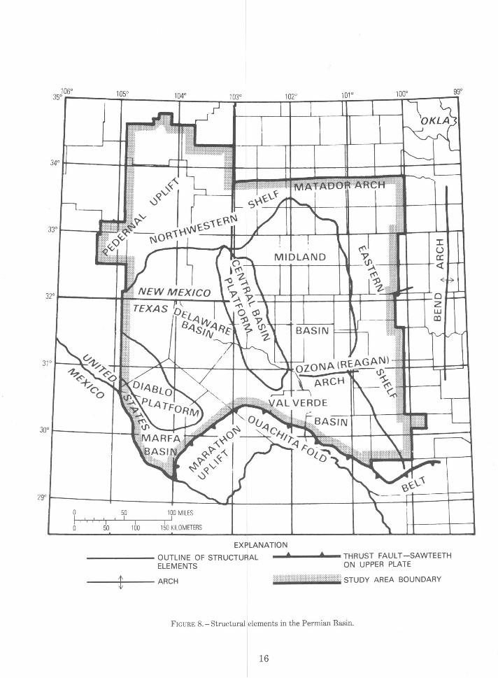
0

0 50 100 150 KILOMETERS

EXPLANATION

------ OUTLINE OF STRUCTURAL ELEMENTS

----+--- ARCH

_....__ ...... ......__THRUST FAULT -SAWTEETH ON UPPER PLATE

hiiJ:ifil!il!ili!i11!'il!t, "" :nw STUDY AREA BOUNDARY

FIGURE 8.- Structural elements in the Permian Basin.

16

remam1ng older Paleozoic systems. Each major stratigraphic unit (such as the Permian, Car­boniferous, and older Paleozoic) was analyzed in­dependently by a team of geologists. Because of restrictions imposed by physical characteristics of each unit, specific methods of data preparation and treatment in each unit vary to a certain degree. However, the objective of the analysis-to assess undiscovered in place hydrocarbons, and the prob­ability distributions for pool sizes containing these hydrocarbons- dictated similar methods of ap­proach for all three units. The separate assessments were combined into the totals reported here.

The procedure for estimating the undiscovered oil and natural gas in the Permian Basin involved an intensive review of the geology and analysis of historical data, and ultimately the application of subjective probability methods for the actual assessment.

GEOLOGIC ANALYSES

All available geologic, drilling, reservoir­engineering, and related data were compiled for the three major stratigraphic units. The Dallas Field Office of the Energy Information Ad­ministration, U.S. Department of Energy (at that time part of the U.S. Bureau of Mines) supplied data concerning total known oil and gas reserves of the Permian Basin, initial oil and gas in place, estimates of ultimate recovery, amounts of associated and dissolved gas, field and pool sizes, discovery dates, age of productive units, depths of production, and general reservoir characteristics. Basic drilling information, derived from the Petroleum Information Corp. "Well History Con­trol System" (unpub. proprietary commercial data file) was used to establish the well density, penetra­tion depths, identification of stratigraphic units, and historical success records of exploratory wells. Publicly available literature provided information on porosities, permeabilities, reservoir lithologies, amounts of net pay sections, gas/oil ratios, hydrocarbon properties, trapping mechanisms, and types of reservoir seals. Literature on the Per­mian Basin, USGS files, and unpublished maps also provided isopach, lithofacies, and some structural maps. Studies on geophysical investigations were not available.

Subsurface geologic maps were prepared for 5,000-foot depth intervals and were used, together with isopach maps, to calculate the total area and volume of the three major stratigraphic units.

17

Volumes of sediment in each of the three major stratigraphic units were partitioned into the depth intervals of 0-10,000, 10,000-20,000, and 20,000-30,000 feet.

Drilling-density maps were prepared and pro­vided the basis for outlining maturely drilled areas, immaturely drilled areas, and totally undrilled areas. Maturely drilled areas are defined as having 12 or more wells per 25 square miles, and im­maturely 'drilled areas as having less than 12, and more than 0, wells per 25 square miles. Combined with rock distributions, these maps provided volumes and areas of maturely drilled, immaturely drilled, and undrilled rock in each major stratigraphic unit and in each depth interval. The drilling-density maps were based on maps of new­field wildcats drilled through or into specific stratigraphic units and were derived from Petroleum Information Corp. "Well History Con­trol System" (unpubl. proprietary commercial data file). To these maps, the locations of oil and gas fields producing from the same or older stratigraphic units were added. The resulting com­bined maps were contoured on the basis of well density.

To gain some idea of the possible range of un­discovered oil and gas in place, we applied yield 4

factors to the volumes or areas of immaturely drilled and undrilled rock. These yield factors were derived from maturely drilled areas of the basin and were applied to sedimentary-rock volumes or areas within individual tectonic elements or on a gross regional scale or trend basis. To calculate a possible "high" amount of undiscovered oil or gas for any one area, we assumed that geologic and reservoir conditions in the immaturely drilled or undrilled areas were similar to those existing in the maturely drilled producing area. Such ~onditions include lithologic and reservoir variables, trap types, sealing mechanisms, and source rocks. We calculated "low" amounts by: (1) reducing the total area or volume of sedimentary rock in immaturely drilled areas by a quantity assumed tested by the exploratory wells in the area, (2) discounting un­drilled or immaturely drilled sedimentary-rock volume in direct proportion to the success ratio established in maturely drilled producing areas before applying the yield factor, or (3) discounting either the undrilled sedimentary-rock volumes or historic-yield factors, assuming particularly un­favorable geologic conditions. Yield factors were directly lowered in some places to reflect a reduced

4 Yield, as used here, applies to in place rather than recoverable quantities.

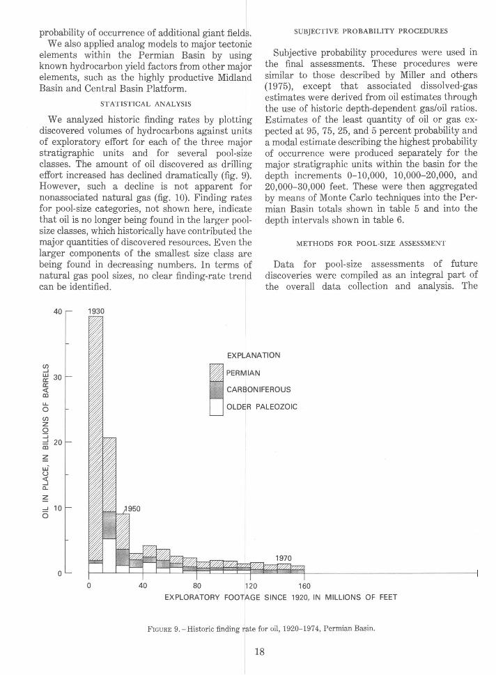
probability of occurrence of additional giant fields. We also applied analog models to major tectonic

elements within the Permian Basin by using known hydrocarbon yield factors from other major elements, such as the highly productive Midland Basin and Central Basin Platform.

STATISTICAL ANALYSIS

We analyzed historic finding rates by plotting discovered volumes of hydrocarbons against units of exploratory effort for each of the three major stratigraphic units and for several pool-size classes. The amount of oil discovered as drilling effort increased has declined dramatically (fig. 9). However, such a decline is not apparent for nonassociated natural gas (fig. 10). Finding rates for pool-size categories, not shown here, indicate that oil is no longer being found in the larger pool­size classes, which historically have contributed the major quantities of discovered resources. Even the larger components of the smallest size class are being found in decreasing numbers. In terms of natural gas pool sizes, no clear finding-rate trend can be identified.

40 1930

SUBJECTIVE PROBABILITY PROCEDURES

Subjective probability procedures were used in the final assessments. These procedures were similar to those described by Miller and others (1975), except that associated dissolved-gas estimates were derived from oil estimates through the use of historic depth-dependent gas/oil ratios. Estimates of the least quantity of oil or gas ex­pected at 95, 75, 25, and 5 percent probability and a modal estimate describing the highest probability of occurrence were produced separately for the major stratigraphic units within the basin for the depth increments 0-10,000, 10,000-20,000, and 20,000-30,000 feet. These were then aggregated by means of Monte Carlo techniques into the Per­mian Basin totals shown in table 5 and into the depth intervals shown in table 6.

METHODS FOR POOL-SIZE ASSESSMENT

Data for pool-size assessments of future discoveries were compiled as an integral part of the overall data collection and analysis. The

EXPLANATION (/) -' ~ 30 a: <X: CD

u.. 0 ~

PERMIAN CARBONIFEROUS .

OLDER PALEOZOIC

(/) z 0 :J -' 20 CD

~ w' u :5 a..

~ ....J 10 0

0

0 40 80 120 160

EXPLORATORY FOOTAGE SINCE 1920, IN MILLIONS OF FEET

FIGURE 9.-Historic finding rate for oil, 1920-1974, Permian Basin.

18

1970

6

EXPLANATION

PERMIAN 1-UJ UJ CARBONIFEROUS u..

~ Ill OLDER PALEOZOIC ::::l 4 u u.. 0 (/)

z Q ...J ...J

a: 1-

~ 1950 UJ-

u ~ 2 ...J 0..

~ (/) ~ t!J

0

0 40 80 120 160

EXPLORATORY FOOTAGE SINCE 1920, IN MILLIONS OF FEET FIGU RE 10.- Historic finding rate for nonassociated natural gas, 1920-74, Permian Basin.

historic pool-discovery data were subjected to several analyses with each major stratigraphic unit.

(1) Histograms were prepared for all pool-size classes by depth intervals and by equal units of exploratory effort.

(2) Cumulative frequency distributions were cal­culated for the entire historic period and for the last two 40-million-foot units of ex­ploratory effort.

(3) A linear regression was fitted to the historic cumulative frequency distributions in an attempt to project numbers and frequen­cies of pools in the very small classes.

(4) Finding-rate curves were calculated for var­ious field-size classes.

Probability estimates of the pool sizes in which the assessed undiscovered oil and nonassociated gas in place occur were produced by subject prob­ability procedures for each of the major strati­graphic units and depth intervals. Pool sizes were

19

estimated as in place quantities. Dissolved and associated gas occurrences were not included in size estimates of those pools.

The evaluators provided estimates of the minimum pool size corresponding to the 95, 75, 25, and 5 percentile probabilities and also of a modal ("most likely") value. Attempts were made to fit several functions to these subjective estimates. Although no totally satisfactory fit was found, a lognormal curve was used. As a result of the lognormal curve, the calcuated mean pool sizes ap­pear unduly large, and the reported distributions should be viewed only as approximations of the assessed distributions of undiscovered pool sizes. Pool-size assessments were made by stratigraphic interval. Aggregations of the pool-size distribu­tions into a basin total are not currently available.

SUMMARY RESULTS

Assessed total undiscovered oil and gas in place are summarized in table 5 and shown by depth

TABLE 5.-Estimates oftotal undiscovered hydrocarbons in place

[The values shown are the estimates corresponding to the probability that there is at least that amount. Values shown are derived from lognormal curve fits at the 0.95 and 0.05 probability levels]

0.95 0.75 0.25 0.05 Mean

Standard probability probability probability probability deviation

Oil in place (109 bbls) ------------------------ 3.32 4.53 7.22 10.43 6.35 2.29

Gas in place (in trillion cubic feet) Dissolved and associated ------------------- 2.99 4.06 6.31 8.83 5.57 1.85 N onassociated --------------------------- 8.24 11.38 18.80 28.27 16.30 6.58

Total --------------·------------------- 12.89 16.50 24.29 33.80 21.87 6.74

TABLE 6. -Estimates of total undiscovered hydrocarbons in place by depth interval

[The values shown are the estimates corresponding to the probability that there is at least that amount. Values shown are derived from lognormal curve fits at the 0.95 and 0.05 probability levels]

Depth interval (thousand feet) 0.95 probability

0.75 probability

0.25 probability

0.05 probability Mean

Standard deviation

Undiscovered oil in place (10 9 bbls)

0-10 ___________________________________ _ 10-20 ___________________________________ _

2.31 .51

3.37 .79

5.91 1.52

8.87 2.56

5.05 1.30

2.18 .69

Undiscovered associated dissolved gas in place (trillion cubic feet)

0-10 ___________________________________ _ 10-20 ___________________________________ _

1.76 .68

2.58 1.07

4.42 2.08

6.70 3.53

3.80 1.77

1.56 .97

Undiscovered nonassociated gas in place (trillion cubic feet)

0-10 ___________________________________ _ 10-20 ___________________________________ _ 20-30 ___________________________________ _

1.43 3.73

.75

interval in table 6. Probability distributions for the data in table 5 are given in figures 11 through 14. Table 7 shows the estimated mean depths of occur­rence for undiscovered hydrocarbons in place by depth intervals for all Paleozoic systems, of 10,000 feet. Examples of the fit of lognormal curves for a few of the pool-size probability distributions, alon$" with dots representing the numerical average d;f original estimates to which the curves have been fitted, are given in figures 15 through 17.

THE DISCOVERY-PROCESS MODEL

Through discovery and production-cost analyses, the number, size, and depth of occurrence of future oil and gas discoveries in the Permian Basin can b~ estimated. Because the Permian Basin has a long exploration history, the pattern of future discoveries may be forecast by extrapolating the past drilling and discovery record.

The method used here to forecast the size distribution of future discoveries is based upon a well-documented and not surprising characteristic of the petroleum-discovery process; the large

20

2.16 6.17 1.28

3.83 12.74

2.73

5.98 21.90 4.86

3.31 10.70 2.29

1.52 6.15 1.38

TABLE 7.-Estimates of mean depths of occurrence of undiscovered hydrocarbons in place-all Paleozoic systems

Depth interval (thousand feet)

0-10 ------------10-20 ------------20-30 ------------

0-30 ------------

[n.a., not applicable]

Mean depth of occurrence (ft)

Oil

6,100 11,800 n.a. 7,300

Nonassociated gas

7,600 15,400 21,500 14,700

deposits tend to be discovered early in the explora­tion of an area (Ryan, 1973; Barouch and Kauf­man, 1978; Drew and others, 1978, 1979; and Arps and Roberts, 1958). Any reasonable quantitative model of the discovery process must incorporate this characteristic. The model described here was proposed by Arps and Roberts (1958) and assumes that the probability of the next exploratory well finding a field of a given area is proportional to the ratio of the area of the field to the area of the basin. Thus, a field having a large surface area has a higher probability of being discovered early than does a field having a small surface area. For this

1.0

~ ~

\ PROBABILITY 0.95: 3.32 billion bbls 0.05: 10.43 billion bbls

0.8

>- 0.6 1-:::::i a:i <( a::l 0 \

Mean: 6.35 billion bbls Standard deviation: 2.29 billion bbls

~

~ "

a: c.. 0.4

0.2

~ r--.___ -0.0 0 2 4 6 8 10 12

RESOURCE IN PLACE, IN BILLIONS OF BARRELS

FIGURE 11.- Probability distribution of the total Paleozoic undiscovered oil in place, aggregated for depths of 0-20,000 feet.

reason, the model initially projects a distribution of the areal sizes of future discoveries. This distribu­tion is then converted into a distribution of the volumes of predicted future recoverable petroleum by relating the average areal size of fields to the average volume of recoverable petroleum that they contain.

This approach was originally devised to forecast future discoveries in a basin having only a single productive horizon without large structural relief. The approach had to be modified before it could be used in a basin, characterized by many productive strata at varying depths and modes of geologic oc­currence (for example, the Permian Basin). To apply the model to the Permian Basin, we divided the basin into four layers, each 5,000 feet thick. Forecasts of future discovery rates were then made independently for each layer.

Two types of information were required for the analysis: (1) detailed information on the ex­ploratory drilling history of the basin, obtained from the Petroleum Information Corp. "Well History Control System" (proprietary unpub.

commercial data file) which gives the completion date and total depth of each exploratory well drilled before January 1, 1975; and (2) information on the known oil and gas fields in the Permian Basin; including the volume of recoverable oil and gas, the discovery, and the depth and surface pro­jection area of each field, prepared by the Dallas Field Office of the Energy Information Adminis­tration, DOE (unpub. data, 1977-78.)

EXPRESSING THE DATA IN DEPTH INTERVALS

The oil and gas fields were divided into four depth-class intervals: 0-5,000, 5,0W)-10,000, 10,000-15,000, and 15,000-20,000 feet. Few data were available for depths greater than 1f,OOO feet. No estimates were made for fields deeper than 20,000 feet because of insufficient data as of December 31, 1974. A field was assigned to the in­terval that contained its largest reservo'r. Within each interval, the fields were partition(\d into 20 size classes based upon quantities of recoverable oil and gas (table 8). "Oil equivalent" ex:[:ressed as BOE (barrels of oil equivalent) repres~nts total

21

1.0

\ '

0.8

~ PROBABILITY 0.95: 2.99 trillion ft3 0.05: 8.83 trillion ft3

~ 0.6 :::; co <( OJ 0 a: a..

0.4 \

Mean: 5.57 trillion ft3 Standard deviation: 1.85 trillion ft3

\

"' ~ 1----~-

0.2

0.0 0 2 4 6 8 10 12

RESOURCE IN PLACE, IN TRILLIONS OF CUBIC FEET

FIGURE 12.- Probability distribution of total Paleozoic undiscovered dissolved and associated gas in place, aggregated for depths of 0-20,000 feet. Pool sizes in trillions of cubic feet (ft3).

volatile hydrocarbon fluids. It includes barrels of oil, barrels of lease condensate, and thousands of cubic feet of wet natural gas converted to BOE. The average volume of recoverable oil equivalent and average areal extent of the fields in each size class and depth interval combination were also computed.

TABLE 8.-Field-size classes [BOE, barrels of oil equivalent]

Size clsss Size range (million BOE recoverable oil and gas)

1 -------------------------------2 -------------------------------3 -------------------------------4 -------------------------------5 -------------------------------6 -------------------------------7 -------------------------------8 -------------------------------9 -------------------------------

10 -------------------------------11 -------------------------------12 -------------------------------13 -------------------------------14 -------------------------------15 -------------------------------16-------------------------------17 -------------------------------18 -------------------------------19 -------------------------------20 -------------------------------

0.0 to 0.006 .006 to .012 .012 to .024 .024 to .047 .047 to .095 .095 to .19 .19 to .38 .38 to .76 .76 to 1.52

1.52 to 3.04 3.04 to 6.07 6.07 to 12.14

12.14 to 24.3 24.3 to 48.6 48.6 to 97.2 97.2 to 194.3

194.3 to 388.6 388.6 to 777.2 777.2 to 1,554.4

1,554.5 to 3,109.0

22

The number of exploratory wells drilled each year was converted into the number of net wells per year within each depth interval. For example, an exploratory well drilled to a total depth of 7,500 feet was counted as one well in the 0-F,OOO-foot in­terval and as half a well in the 5,000-10,000-foot interval. A well drilled to a total depth of 20,000 feet was counted as one well in each of the four depth intervals.

FORM OF THE MODEL

The discovery-process model select(ld to predict future rates of discovery in the Permian Basin has the following analytic form for relating discoveries to exploratory wells:

Fa (w)=Fa ( 00) * (1- e-CAw/B~

where:

Fa (w)=the cumulative number of discoveries estimated to be made in size class a by the drilling of w exploratory wells,

Fa ( oo) =the ultimate number of fields in size class A that occur within the b~sin,

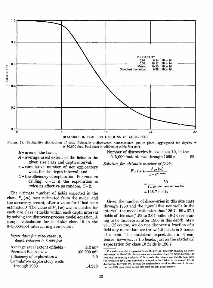
1-or-------=-;;==--,---------------~----------------r-----------------

o.ar----------------+----~----------+---------------~----------------~

PROBABILITY 0.95: 8.24 trillion ft3 0.05: 28.27 trillion ft3

Mean: 16.30 trillion ft3 ~ o.sr------------------+----------~~----~--------Standard deviation: 6.58 trillion ft3 1-

:J iil <( OJ 0 a: c.. 0.4.---------------4---------------~~--------------~--------------~

0.2r----------------+----------------+-------~~----~----------------~

0.00~--------------~----------------~--------------~----------------~ 8 16 24 32

RESOURCE IN PLACE, IN TRILLIONS OF CUBIC FEET

FIGURE 13. -Probability distribution of total Paleozoic undiscovered nonassociated gas in place, aggregated for depths of 0-30,000 feet. Pool sizes in trillions of cubic feet (ft3).

B =area of the basin, A= average areal extent of the fields in the

given size class and depth interval, w =cumulative number of net exploratory

wells for the depth interval, and C =the efficiency of exploration. For random

drilling, C= 1; if the exploration is twice as effective as random, C = 2.

The ultimate number of fields expected in the class, Fa ( oo ), was estimated from the model and the discovery record, after a value for C had been estimated. 5 The value of Fa ( oo) was calculated for each size class of fields within each depth interval by solving the discovery-process model equation. A sample calculation for field-size class 10 in the 0-5,000-foot interval is given below:

Input data for size- class 10, depth interval 0-5,000 feet

Average areal extent of fields= Permian Basin size= Efficiency of exploration= Cumulative exploratory wells

through 1960 =

2.2 mi2

100,000 mi2 2.0

14,243

23

Number of discoveries in size-class 10, in the 0-5,000 foot interval through 1960= 59

Solution for ultimate number of fields

FlO ( oo) FlO (w) 1-e-CAw/B

59 1- e-2.0.2.2. l4.243/too.ooo

= 126.7 fields

Given the number of discoveries in this size class through 1960 and the cumulative net wells in the interval, the model estimates that 126.7- 59= 67.7 fields of this size (1.52 to 3.04 million BOE) remain­ing to be discovered after 1960 in this dep-l:h inter­val. Of course, we do not discover a fraction of a field any more than we throw 1.5 heads in 3 tosses of a coin. The statistical expectation ir 3 coin tosses, however, is 1.5 heads, just as the statistical expectation for class 10 fields is 126.7.

5 For each value of Cit is possible to use the pre-1961 discovery data and the model to forecast the 1961-1974 discoveries in each size class in a given deptli interval. The criterion for selecting a value for C for a particular interval was that the total oil in the forecasted 1961-1974 discoveries be equal to the total oil in the adual 1961-74 discoveries. The value of C selected for a particular interval was then UF"d to forecast the post·1974 discoveries in each size class for that depth interval.

1.0

~ 0.8

>- 0.6 1-:::::i cc <{ m 0 a: a..

0.4

0.2

~ PROBABILITY

0.95: i 2.89 trillion ft3 0.05: 23.80 trillion ft3

Mean: ~1.87 trillion ft3 Standard deviation: 6.74 trillion ft3

\ ""' ~ "',

,,~

8 16 24 32 RESOURCE IN PLACE, IN TRILLIONS OF CUBIC FEET

FIGURE 14.-Probability distribution of total Paleozoic undiscovered gas (dissolved, associated, nonassociated) in p1ace, aggregated for depths of 0-30,000 feet. Pool sizes in trillions of cubic feet (ft3

).

TABLE 9.-Compa·rison of the numbers ofd·iscoveries through 1974 with the number forecast, keyed on the pre-1!?61 discovery and explora.tory driZZ.ing data ·in the 0-5,000joot depth interval

Size class

2 -----------------------

6 -----------------------7 -----------------------8 -----------------------!J -----------------------

10 -----------------------11 -----------------------12 -----------------------13 -----------------------14 -----------------------15 -----------------------16 -----------------------17 -----------------------H! -----------------------1!! -----------------------20 -----------------------

Area (square miles)

0.13 .14 .16 .22 .25 .39 .49 .94

1.23 2.21 4.2-1 5.40 8.30

18.19 40.42 49.19 67.20 81.75

12!!.88 40.25

Actual

211 84 84 92

127 135 129 104 111 84 75 49 35 1!J 14 16 9

Total ---------------------------- ------------------------- 1,387

We can determine whether an estimate arrived at by means of this method is reasonable by mak­ing an historical forecast from 1960 to some subse­quent year before 1979. The forecast can then be checked against the actual number of discoveries

24

Discoveries

Estimated Difference

200.1 lO.!J 66.0 18.0 8-1.7 - .7 67.0 25.0

10!!.6 17.4 114.8 20.2 125.3 3.7 92.8 11.2

107.4 3.6 84.5 - .5 82.9 -7.!! 52.2 -3.2 33.3 1.7 18.2 .8 14.0 .0 16.0 .0 9.0 .0 6.0 .0 2.0 .0 1.0 .0

1,286.8 100.2

made in the field-size class from 19fl) to that par­ticular year. The forecast shown t~low projects discoveries for size-class 10. On the l"~.sis of 25,055 wells drilled in the 0-5,000-foot interval from the start of exploration through 1974,

1.0

0.8

~ ~ 0.6 m <(

~ 0.4 a: a..

0.2

0

1.0

0.8

>­I-:;;;! 0.6 m <( m 0 0.4 a: a..

0.2

)

)

\_

~

)

\ "-

0-1o.boo tt -,

PROBABILITY 0.95: 0.002 million bbls 0.05: 15.481 million bbls

~ r---

_I I I 1o.ooo.-r.ooo

1

ft

PROBABILITY 0.95: 0.001 million bbls 0.05: 5.769 million bbls

r----o

1.0

0.8

~ ::::i 0.6 iii <( m ~ 0.4 a..

0.2

0

1.0

0.8

~ ~ 0.6 iii <( co ~ 0.4 a..

0.2

)

\

\ .............. ---

C)

)

\ ............ 1---

_I ~

110.0001 PROBABILITY

0.95: 0.002 million bbls 0.05: 11.121 million bbls

f..-- ,.... -

_I_ I

10,0,00-20,0010 ft

PROBABILITY 0.95: 0.002 million bbls 0.05: 8.336 million bbls

,....

0 0 4 8 12 16 20 2 4 6 8 10 12 14

POOL SIZE, IN MILLIONS OF BARRELS

FIGURE 15.- Lognormal-probability size distribution of undis­covered Permian oil pools in depths of 0-10,000 and 10,000-20,000 feet.

F 10 (25055) = 126.7 * {1- e-z.o.2.2.25o55ttooooo)

= 84.5 deposits to be discovered by 12/31/74

As 59 discoveries in this size class had been made by 1960, the model is forecasting an additional 84.5-59.0=25.5 fields in class 10 to be discovered between 1960 and 1974. In fact, 25 discoveries were made in the size class during the 15-year period, so the model produced a remarkably ac­curate forecast. The results of analogous calcula­tions for other classes are presented in table 9. The level of accuracy varies among the field-size classes and also across the depth intervals. In general, however, acceptable agreement was found be­tween the predicted and the acutal levels of discoveries.

The major differences between the actual and predicted number of discoveries in the 0-5,000-foot depth interval were found in six of the eight smallest size classes (table 9). In each of these six size classes, the model underpredicted the actual level of discovery. These underpredictions oc­curred because the rate of discovery in these small

25

POOL SIZE, IN MILLIONS OF BARRELS

FIGURE 16.- Lognormal-probability size distributio'1 of undis­covered Carboniferous oil pools in depths of 0-10,000 and 10,000-20,000 feet.

size classes accelerated during the 1961-74 time period in comparison with the pre-1961 rates of discovery. The consequence of these underpredic­tions is small, however, because most of tl:le fields involved contain relatively small amo'lnts of petroleum.

FORECASTING FUTURE RATES OF RECOVERY

Forecasts of the number of discoveries within each field-size class and depth interval were made for 20 increments of drilling, each consisting of 1,000 exploratory wells at the surface. Within each of these drilling increments, a portion of the. wells on a net-well basis was applied against the ex­pected size distribution of fields remaining to be discovered at the start of each drilling inc':'ement. The assignments of the net wells to be drilled in each drilling increment were taken from extrapola­tions of the historical trends in the net-well penetration in each depth interval versus the cumulative wells drilled at the surface through 197 4. A mathematical function was fitted to each of these net-well curves and then extrapolated for

1.0

> 0.8 ....

~ l ~1o,ro ft

I ~ 0.6 co ~ co 0.4 0 cr: a. 0.2

PROBABILITY 0.95: 0.003 billion ft3

\ 0.05: 53.081 billion ft3

\o ' 1'---..

"""' 0 0 20 40 60

POOL SIZE, IN BILLIONS OF CUBIC FEET

1.0

> 0.8 ....

4) l 10.~~0,000 ft

I ~ 0.6 co

PROBABILITY 0.95: 0.003 billion ft3

~ 0.05: 46.708 billion ft3 co 0.4 0 cr: a. 0.2 ~

' ......_ .....

0 0 20 40 60

POOL SIZE, IN BILLIONS OF CUBIC FEET

1.0

> 0.8 ....

)

DEJPER THfN 20,~0 ft ) I I

~ 0.6 co

PROBABILITY 0.95: 0.001 billion ft3

~ 0.05: 32.107 billion ft3 co 0.4 0 cr: a. 0.2 \>

"'--. -0 -

0 20 40 60 POOL SIZE, IN BILLIONS OF CUBIC FEET

FIGURE 17.-Lognormal-probability size distribution of undis­covered nonassociated Carboniferous gas pools in depths of 0-10,000, 10,000-20,000, and deeper than 20,000 feet.

an additional20,000 exploratory wells to be drilled in the future.

The number of deposits expected to be discovered within each field-size class for any future increment of exploratory drilling can be determined by aggregating the expected number of discoveries to be made within each depth inter­val. The first increment of 1,000 exploratory wells drilled at the surface results in 900 net wells in the

26

0-5,000-foot interval, 500 net wells in the 5,000-10,000-foot interval, 130 net wells in the 10,000-15,000-foot interval, and 35 net wells in the 15,000-20,000-foot interval. The expected size distribution of fields remaining to be discovered at the start of the first drilling incremE'llt within each of the four depth intervals is shown in tables 10 through 13.

The number of discoveries (150.9) forecast within the first 1,000-well increment is giv~n in table 14. The largest discovery is predicted in class 17 (194.3 to 388.6 million BOE). This discove':"y (in expecta­tion, 0.1 fields) is predicted to be in the 15,000-20,000-foot depth interval. VTith the excep­tion of class 1, the largest number of discovered fields within a single field-size class is expected to occur with class 7 (0.19 to 0.38 million BOE), where a total of 16.7 discoveries are expected to be made within all four of the depth intervals.

Comparing the expected number of discoveries across the depth intervals reveals a trend in the forecast sizes of discoveries. In the shallowest, most highly explored depth interval, no discoveries are expected to be larger than field-size class 12 (6.07 to 12.14 million BOE); in the se~ond and third depth intervals, discoveries are e:rpected to be made to size class 15; and in the deApest interval, discoveries are expected in size claFses 16 and 17 during the first drilling increment.

A similar table can be made for each of the in­crements of exploratory drilling. A comparison made across the successive drilling increments in­dicates that the total number of disc-:weries per in­crement is projected to decline grad·.1ally and that the larger discoveries are projected to become less frequent. Thus, both the success rath and average size of the discoveries are projected t.o decline with each successive increment of exploratory drilling.

CONCLUSIONS

The discovery-process model pr1~dicts that a large number of oil and gas fields remains to be discovered- approximately 34,000 fields in the basin at depths shallower than 20,000 feet- but that most of these fields individually contain very small volumes of oil and gas, as the following tabulation shows:

Field size (millions of barrels of oil equivalent)

48.6 and larger ______ _ 12.14 to 48.6 ________ _

1.52 to 12.14 _______ _

Number

6.6 20.7

681.6

Percentage of total remaining fields

0.02 0.06 2.00

TABLE 10.-Expected ultimate number of fields remaining to be discovered after 1971,. in the 0-5,000joot depth interval

Size class

1 -------------------------------2 -------------------------------3 -------------------------------4 -------------------------------5 -------------------------------6 -------------------------------7 -------------------------------8 -------------------------------9 -------------------------------

10 -------------------------------11 -------------------------------12 -------------------------------13 -------------------------------14 + -----------------------------

Area (square miles)

0.13 .14 .16 .22 .25 .39 .49 .94

1.23 2.21 4.24 5.40 8.30

46.18

Expected number of Number of fields fields remaining found by 197 4

4,106.1 211 1,355.3 84 1,006.3 84

789.4 9Z 951.6 127 625.5 135 463.5 12r 175.2 10~

130.3 111 41.4 84-10.2 75 2.5 4r

.1 35

.0 67

TABLE 11.-Expected ultimate number of fields remaining to be discovered after 1971,. in the 5,000-10,000joot depth interval

Size class

6 -------------------------------7 -------------------------------8 -------------------------------9 -------------------------------

10 -------------------------------11 -------------------------------12 -------------------------------13 -------------------------------14 -------------------------------15 -------------------------------16 + - ----------------------------

Area (square miles)

0.12 .12 .13 .19 .20 .29 .42 .47 .76

1.28 2.21 3.76 5.40

10.86 20.30 72.14

Expected number of Number of fields fields remaining found by 197 4

5,462.9 21f 2,922.0 11f 2,856.8 12~

2,189.6 13f 2,468.0 164 1,718.2 16f 1,382.6 20(

751.6 16( 570.5 15f 245.4 1 '"'

94.6 9f 26.6 7f

5.9 5(

1.5 47 .2 27 .0 27

TABLE 12.-Expected ulh:mate number of fields remaining to be disco'vered after 1971,. in the 10,000-15,000-foot deptf., interval

Size class

2 -------------------------------3 -------------------------------4 -------------------------------5 -------------------------------6 -------------------------------7 -------------------------------8 -------------------------------9 -------------------------------

10 -------------------------------11 -------------------------------12 -------------------------------13 -------------------------------14 -------------------------------15 -------------------------------16 + -----------------------------

Area (square miles)

0.21 .22 .33 .25 .31 .37 .31 .43 .63

1.30 1.20 1.90 3.89 4.77 7.53

12.67

27

Expected number of Number of fields fields remaining found by 1974

511.0 49 307.9 31 277.2 36 400.7 56 320.6 48 302.7 53 325.4 62 249.1 54 196.1 62 97.8 47 93.1 64 34.5 4f

6.3 28 1.6 21

.3 18

.0 r

TABLE 13.-Expected ultirnate number offields remaining to be discovered ajler 1974 in the 15,000-20,000joot depth interva.l 1

S1ze elass

•J -------------------------------3 -------------------------------4 -------------------------------5 -------------------------------

9 -------------------------------10-------------------------------11 -------------------------------12 -------------------------------13 -------------------------------14 -------------------------------15 - ------------------------------16 -------------------------------17 -------------------------------18 -------------------------------

Area (square miles)

1.00 1.00

.00 1.00 1.00 .78

1.00 .25

1.00 2.25 3.67 4.00 4.50 9.00

10.50 9.00

21.00 14.00

Expected number of Number o~ fields fields remaining found by 1974

17.6 17.6

.0 0 26.5 3 17.6 35.3 17.6 8.8 1 8.8 1

22.9 4 10.7 3

1.9 1 2.7 2 2.6 3 5.5 9

.3 1

.2 1

.1 1

1 The USGS resource appraisal group estimated that no oil, and a mean value of 2.29 trillion cubic feet of gas in place, exists below 20,000 feet.

TABLE 14.-Nurnber of discoveries expected to be made in each size class with the .first ·increment of 1,000 explo'ratory holes drated in the Permian Basin after 1974

Size class

3 -------------------------------------------------4 -------------------------------------------------5 -------------------------------------------------

9 -------------------------------------------------10 ---------------------- ---------------------------11 -------------------------------------------------12 -------------------------------------------------13 -------------------------------------------------14 -------------------------------------------------15 ---------- ---------------------------------------16 ------ -------------------------------------------17 + -----------------------------------------------­

0-5,000-foot depth

7.5 3.0 2.9 39 4.3 4.4 4.1 3.0 2.9 1.6

.8

.3

.0

.0

.0

.0

.0

5,000-10,000-foot depth

10.1 5.4 5.7 6.4 7.6 7.7 8.9 6.9 6.6 4.8 3.2 1.7

.6

.2

.1

.0

.0

10,000-15,000- 15,000-20,000- Total foot depth foot depth

2.8 0.3 20.7 1.7 .3 10.4 2.0 .0 10.6 3.1 .4 13.1 2.6 .3 14.8 2.9 .5 15.5 3.4 .3 16.7 2.!:1 .1 12.9 3.2 .1 12.8 2.3 .5 9.2 2.8 .4 7 •)

1.7 .1 3.8 .6 o) 1.4 .2 .3 .7 .1 .7 .9 .0 .0 .1 .0 .1 .1

38.0 75.9 32.3 4.7 150.9 T··~l ------------------------------------------~~~~~~~~~~~~~~~~~~~.~~~~~~~~~~

The model, thus, predicts that 97.9 percent of the oil and gas fields remaining to be discovered in the Permian Basin individually contain less than 1.52 million BOE.

Furthermore, the model predicts that nearly all the expected fields remaining to be discovered that contain more than 48.6 million BOE each are expected to be in the 15,000-20,000-foot depth in­terval. In contrast, the 20.7 fields remaining to be discovered that individually contain between 12.14 and 48.6 million BO E are expected to occur in approximately equal numbers in the 5,000-10,000-foot, 10,000-15,000-foot, and 15,000-20,000-foot depth intervals. The bulk of the smaller oil and gas fields expected to remain in the basin are predicted by the model to be at depths shallower than 10,000 feet.

28

A prediction of the rate at which t~ese oil and gas fields will be discovered in the future was made for 20 successive future 1,000-well in~rements of exploratory drilling. The predicted s:ze distribu­tion of discoveries to be made in each of these drill­ing increments forms one of the basic inputs into the economic analysis discussed in "E~ngineering and Cost Analysis for Future Fields", and "The In­tegrating Economic Model."

ENGINEERING AND COST ANALYS~S FOR

FUTURE FIELDS

The costs of oil and gas reserve:" from un­discovered fields were estimated by an engineering and cost-analysis model. The model e~timated the exploration, development, and producf0n costs for

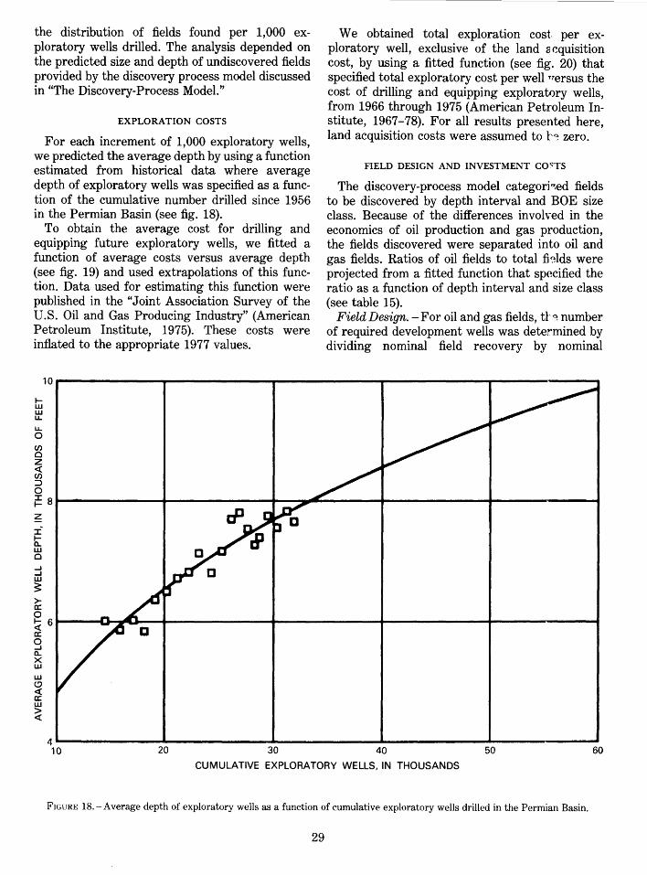
the distribution of fields found per 1,000 ex­ploratory wells drilled. The analysis depended on the predicted size and depth of undiscovered fields provided by the discovery process model discussed in "The Discovery-Process Model."

EXPLORATION COSTS

For each increment of 1,000 exploratory wells, we predicted the average depth by using a function estimated from historical data where average depth of exploratory wells was specified as a func­tion of the cumulative number drilled since 1956 in the Permian Basin (see fig. 18).

To obtain the average cost for drilling and equipping future exploratory wells, we fitted a function of average costs versus average depth (see fig. 19) and used extrapolations of this func­tion. Data used for estimating this function were published in the "Joint Association Survey of the U.S. Oil and Gas Producing Industry" (American Petroleum Institute, 1975). These costs were inflated to the appropriate 1977 values.

We obtained total exploration cost per ex­ploratory well, exclusive of the land acquisition cost, by using a fitted function (see fig. 20) that specified total exploratory cost per well nersus the cost of drilling and equipping exploratory wells, from 1966 through 1975 (American Petroleum In­stitute, 1967-78). For all results presented here, land acquisition costs were assumed to l'~ zero.

FIELD DESIGN AND INVESTMENT CO"TS

The discovery-process model categori~ed fields to be discovered by depth interval and BOE size class. Because of the differences involved in the economics of oil production and gas production, the fields discovered were separated into oil and gas fields. Ratios of oil fields to total fhlds were projected from a fitted function that specified the ratio as a function of depth interval and size class (see table 15).

Field Design. -For oil and gas fields, tl'~ number of required development wells was determined by dividing nominal field recovery by nominal

10P--------------r--------------r--------------r--------------r-------------~ 1-w w LL

LL 0 en 0 z <( en :::> 0

~ s~------------~--------------~~~~------~--------------~------------4 ~ ::C ~ w 0 ....J ....J w ~ >­a: 0 ~ 6~----~~~--~--------------~------------~--------------~------------4 a: 0 ....J a.. X w w (!) <( a: w > <(

~~o------------~2~o--------------3~o--------------4~o--------------5~o------------~6o CUMULATIVE EXPLORATORY WELLS, IN THOUSANDS

FIGURE 18.-Average depth of exploratory wells as a function of cumulative exploratory wells drilled in the Permian Basin.

29

5 10 15

WELL DEPTH, IN THOUSANDS OF FEET

FIGURE 19.- Exploratory well drilling and equipping costs as a function of well depth in the Permian Basin in 1975 (1977 costs can be obtained by increasing by 18.9 percent).

1 2 3 4 5 6 7 8 9

10 11 12 13 14 15 16 17 18 19 20

TABLE 15.-Ratio of oil fields to total fields in the Permian Basin

Size class 0-5,000- 5,000-10,000- 10,000-15,000-foot depth foot depth foot depth

----------------------- 0.86 0.84 0.54 ----------------------- .78 .78 .51 ----------------------- .72 .73 .49 ----------------------- .68 .69 .47 ----------------------- .65 .67 .45 ----------------------- .65 .66 .43 ----------------------- .65 .66 .41 ----------------------- .67 .67 .40 ----------------------- .70 .69 .39 ----------------------- .73 .71 .37 ----------------------- .77 .73 .36 ----------------------- .81 .76 .36 ----------------------- .86 .79 .35 ----------------------- .90 .82 .35 ----------------------- .94 .85 .35 ----------------------- .97 .87 .34 ----------------------- 1.0 .89 .35 ----------------------- 1.0 .90 .35 ----------------------- 1.0 .91 .35 ----------------------- 1.0 .90 .36

reserves per well. We estimated the nominal values for fields under primary recovery only by extrapolating :fitted curves (reserves versus size class), which we estimated by using historical· values from those fields that have undergone primary production only. We used a similar pro­cedure for determining reserves per producing

30

TABLE 16.-Expected ultimate oil recovery per field in the Permian Basin

Size class

1 -----------------------2 -----------------------3 -----------------------4 -----------------------5 -----------------------6 -----------------------7 -----------------------8 -----------------------9 -----------------------

10 -----------------------11 -----------------------12 -----------------------13 -----------------------14 -----------------------15 -----------------------16 -----------------------17 -----------------------18 -----------------------19 -----------------------20 -----------------------

[Million barrels)

0-5,000-foot depth

0.002 .007 .013 .027 .054 .108 .216 .433 .868

1.740 3.500 7.010

14.100 28.200 56.700

114.000 228.000 458.000 918.000

1,840.000

5,000-10,000 10,000-15,000-foot depth foot depth

0.002 .005 .011 .022 .044 .090 .181 .367 .741

1.500 3.030 6.130

12.400 25.000 50.600

102.000 207.000 418.000 846.000

1,710.000

0.002 .005 .011 .021 .042 .084 .166 .330 .656

1.300 2.590 5.150

10.200 20.300 40.400 80.300

160.000 317.000 630.000

1,250.000

well and ultimate recovery for (1) oil fhlds suscep­tible to secondary recovery and (2) nonassociated gas fields. These basic data are presented in tables 16-22. For completeness, values were included for oil fields deeper than 15,000 feet where no historical oil fields existed. Ultimate oil recovery

1000~----------~-------------r------------.-----------~r-------·-----,

.....1

.....1 w ~

t-~ffi

~c..

800~----------~------------+------------t------------t---------~~

(.)(/)

z a: 600 o::S i=o ~Q Ou.. i[o X (f.)

wo •-----------------+-------------~~~:_--------------1-----------------1-----------------1 .....1 z 400 .. << I- (f.) O::J t-o

::I: 1-

~

0 oL_ ____________ 1L00------------~2~0~0------------3~0~0~----------~4~00~----------~500 DRILLING AND EQUIPPING COSTS, IN THOUSANDS OF DOLLARS PER WELL

FIGURE 20. -Total exploration cost per exploratory well (minus cost of acquiring undeveloped acreage) as a function of drilling cost per well in 1977.

TABLE 17.-Expected ultimate oil recovery per well from primary oil fields in the Permian Basin

[Thousand barrels)

Size class 0-5,000- 5,000-10,000- 10,000-15,000-foot depth foot depth foot depth

1 ----------------------- 1.490 1.930 2.160 2 ----------------------- 4.280 4.070 4.170 3 ----------------------- 7.580 8.670 9.590 4 ----------------------- 11.800 15.900 18.900 5 ----------------------- 17.300 25.900 32.400 6 ----------------------- 24.500 39.000 50.700 7 ----------------------- 33.800 55.100 74.100 8 ----------------------- 45.700 74.600 103.000 9 ----------------------- 53.300 82.900 136.000

10 ----------------------- 54.900 118.000 198.000 11 ----------------------- 68.900 132.000 261.000 12 ----------------------- 95.600 140.000 333.000 13 ----------------------- 135.000 154.000 419.000 14 ----------------------- 188.000 189.000 526.000 15 ----------------------- 254.000 258.000 662.000 16 ----------------------- 334.000 374.000 834.000 17 ----------------------- 428.000 550.000 1,050.000 18 ----------------------- 536.000 802.000 1,310.000 19 ----------------------- 658.000 1,140.000 1,630.000 20 ----------------------- 794.000 1,580.000 2,010.000

per field and ultimate gas recovery per well were projected, and ultimate oil recovery per well was set equal to the same value as the 10,000-15,000-foot interval values.

31

TABLE 18. -Expected ultimate associated-dissolved gas recovery per oil well from primary fields in the Permian Basin

[Million cubic feet at 14.73 psia (pounds per square inch absolute) and 60° F)

Size class 0-5,000- 5,000-10,000- 10,000-15,000-foot depth foot depth foot depth

1 ----------------------- 1.490 4.320 7.470 2 ----------------------- 4.740 9.210 14.400 3 ----------------------- 9.050 20.100 32.000 4 ----------------------- 15.200 38.400 63.000 5 ----------------------- 24.100 65.700 110.000 6 ----------------------- 36.500 103.000 175.000 7 ----------------------- 53.200 153.000 261.000 8 ----------------------- 75.100 216.000 371.000 9 ----------------------- 81.900 266.000 506.000

10 ----------------------- 117.000 327.000 657.000 11 ----------------------- 164.000 389.000 806.000 12 ----------------------- 223.000 453.000 1.070.000 13 ---------------------- 293.000 518.000 1.460.000 14 ----------------------- 374.000 584.000 1.960.000 15 ----------------------- 467.000 652.000 2,580.000 16 ----------------------- 572.000 721.000 3 320.000 17 ----------------------- 688.000 1,080.000 4.170.000 18 ----------------------- 816.000 1,570.000 5 150.000 19 ----------------------- 955.000 :~.240.000 6 240.000 20 ----------------------- 1,110.000 :J,100.000 7,450.000

For technical reasons, secondary-r€~overy techniques are not applicable to some oil £Blds. A ratio of primary oil fields to total oil fields was derived for each size and depth class of oil field.

TABLE 19. -Expected ultimate ail rerovery per weU from secmulJJ,ry arui ']Jf'eSSUre maintenance fields in the Permian Basin

[Thousand barrels)

Size class 0-5,000- 5,000-10,000- 10,000-15,000-foot depth foot depth foot depth

1 -----------------------2 -----------------------3 -----------------------4 -----------------------5 -----------------------6 ----------------------- 12.500 41.500 7 ----------------------- 20.300 49.100 8 ----------------------- 28.500 58.400 9 ----------------------- 37.200 69.500 107.000

10 ----------------------- 46.300 82.300 131.000 11 ----------------------- 55.800 96.900 154.000 12 ----------------------- 65.800 161.000 178.000 13 ----------------------- 76.300 176.000 202.000 14 ----------------------- 87.200 186.000 336.000 15 ----------------------- 99.600 219.000 484.000 16 ----------------------- 129.000 304.000 648.000 17 ----------------------- 195.000 456.000 828.000 18 ----------------------- 298.000 624.000 1,020.000 19 ----------------------- 438.000 831.000 1,230.000 20 ----------------------- 614.000 1,070.000 1,460.000

TABLE 20.-Expected ultimate gas recovery per oil well from secondary and pressure maintenance fields in the Permian

Basin

[Million cubic feet at 14.73 psia (pounds per square inch absolute) and 60° F]

Size class

1 -----------------------2 -----------------------3 -----------------------4 -----------------------5 -----------------------6 -----------------------7 -----------------------8 -----------------------9 -----------------------

10 -----------------------11 -----------------------12 -----------------------13 -----------------------14 -----------------------15 -----------------------16 -----------------------17 -----------------------18 -----------------------19 -----------------------20 -----------------------

0-5,000-foot depth

12.000 23.400 34.900 46.300 57.800 69.200 80.600 92.100

104.000 122.000 145.000 185.000 242.000 315.000 405.000

5,000-10,000-foot depth

93.500 111.000 136.000 168.000 208.000 254.000 374.000 400.000 420.000 452.000 514.000 622.000 796.000

1,050.000 1,410.000

10,000-15,000-foot depth

348.000 464.000 580.000 695.000 811.000

1,360.000 1,910.000 2,470.000 3,020.000 3,580.000 4,100.000 4,680.000

TABLE 21.-Expected ultimate nona.ssociated gas reco·very per· .field in the Perm·ian Basin

[Million cubic feet at 14.73 psia (pounds per square inch absolute) and 60° F]

Size class 0-5,000- 5,000-10,000- 10,000-15,000- Greater than foot depth foot depth foot depth 15,000-foot depth

1-4 86 102 95 102 5 366 347 334 286 6 704 720 756 839 7 1,364 1,412 1,412 1,269 8 2,670 2,991 2,836 3,234 9 5,544 5,418 5,130 5,562

10 11,206 11,368 10,773 10,989 11 20,760 21,690 20,560 26,528 12 47,355 48,735 46,554 43,860 13 95,245 85,407 86,184 96,964 14 185,319 186,912 180,455 160,376 15 361,284 3!:l0,010 400,842 359,114 16 714,015 554,960 713,600 852,826 17 1,490,688 1,452,192 1,278,025 1,935,413 18 2,889,936 2,634,969 2,645,554 3,341,724 19 6,140,000 6,140,000 6,140,000 6,140,000 20 12,300,000 12,300,000 12,300,000 12,300,000

32

TABLE 22.-Expected ultimate nonassociated gas recovery per well in the Permian Basin

[Million cubic feet at 14.73 psia (pounds per square inch absolute) and 60° F)

Size class 0-5,000- 5,000-10,000· 10,000-15 000- Greater than foot depth foot depth foot derth 15,000-foot depth

1-4 86 51 95 102 5 183 347 334 286 6 352 360 756 839 7 341 706 706 1,269 8 -------- 445 997 1,418 1,617 9 504 1,357 2,565 2,781

10 862 1,624 3,591 3,663 11 1,038 2,169 5,140 6,632 12 1,155 2,565 7,759 10,965 13 2,215 4,067 12,312 13,852 14 3,141 5,841 16,405 20,047 15 4,301 9,070 22,269 25,651 16 5,805 13,874 28,544 32,801 17 7,764 25,932 36,515 41,179 18 10,248 28,333 45,613 49,143 19 10,248 28,333 45,rJ3 49,143 20 10,248 28,333 45,fl.3 49,143

This ratio was used to apportion oil fields to be discovered into: (1) fields susceptible to primary recovery alone, and (2) fields susceptible to both primary and secondary recovery. Tr~se ratios are presented in table 23.

TABLE 23.-Ratio of primary oil .fields to total oil fields in the Perrnia.n Ba.sin

Size class

1 -----------------------2 -----------------------3 -----------------------4 -----------------------5 -----------------------6 -----------------------7 -----------------------8 -----------------------9 -----------------------

10 -----------------------11 -----------------------12 -----------------------13 -----------------------14 -----------------------15 -----------------------16 -----------------------17 -----------------------18 -----------------------19 -----------------------20

0-5,000-foot depth

1.000 1.000 1.000 1.000 1.000

.984

.958

.891

.781

.636

.474

.318

.188

.097

.048

.030 ,025 .013 .000 .000

5,000-10,000- 10,000-15,000-foot depth foot depth

1.000 1.000 1.000 1.000 1.000 1.000 1.000 1.000 1.000 1.000

.986 1.000

.983 1.000

.972 1.000

.940 .981

.881 .962

.792 .938

.679 .895

.554 .818

.429 .693

.315 .515 ,213 .307 .119 .116 .032 .001 .000 .000 ,000 .000

Depth intervals were: (1) 0-5,000 feet, (2) 5,000-10,000 feet, (3) 10,000-15,000 feet, and (4) greater than 15,000 feet. Average depths (based on historical data) for oil fields correspond­ing to each interval were: (1) 3,400, (2) 7,200, (3) 11,400, and (4) 16,000 feet (no historical fields). The average depths for nonassociated gas fields were: (1) 3,400, (2) 7 ,200, (3) 12,200, and (4) 17,700 feet.

For those fields susceptible to secondary­recovery methods, the design and assumptions of the recovery program depended on the field's depth interval.

(1) In the 0-5,000-foot interval, the primary pro­ducing wells were assumed to constitute 70 percent of all the wells that produced oil. In the secondary-recovery program, the re­maining 30 percent of the producing wells were drilled, and a sufficient number of primary producing wells were converted to injection wells so that there was one injec­tion well for each producing well.

(2) For the interval between 5,000 and 10,000 feet, the number of newly drilled injection wells is given by the relationship:

WNI=((PH)'12 -1)2

where WNI is the number of newly drilled injection wells and PH is the number of primary producing wells. This relationship provides the number of wells needed to infill drill the centers of a square array of wells that produced during the primary stage. The number of primary producers that must be converted to injection wells is such that there is a one-to-one ratio of pro­ducing to injection wells during secondary recovery.

(3) In the two intervals deeper than 10,000 feet, it is assumed that a pressure maintenance program was carried out from the initial stage of development. For each set of four primary producing wells, an injection well was drilled.

Investment Costs.- We estimated drilling and equipping costs for production wells, and dry-hole costs, using data taken from the "Joint Association Survey of the U.S. Oil and Gas Producting In­dustry" (American Petroleum Institute, 1975). Drilling costs were inflated to attain mid-1977 cost levels. The drilling and equipping costs were

expressed as a fitted function of depth. Figures 21 and 22 present the estimated functions.

Costs of dry development wells for all fields were included by increasing costs of each producing well by 19 percent of the cost of a dry hole. Using the U.S. data from 1971 through 1975, we found that the ratio of dry to successful development 'vells did not depend strongly on depth; therefore, the average ratio for all depths was used.

Cost estimates for field lease equipme'l.t were based on data from Dietzman, Pierce, Funk, and Anderson (1978). Costs of oil-field lease eq'Iipment were expressed as a function of well depth (see fig. 23). The cost curve shown in figure 23 is derived from a combination of rod-pumped operatjons to a maximum of 8, 000 feet, and hydraulically pumped operations from 8,000 to 12,000 feet. Costs of nonassociated gas-field equipment were eYoressed as a function of well depth and field size (f~e table 24).

PRODUCTION SCHEDULES AND PRODUCTION COSTS

Production Schedules.- Size classes for all fields were based on a BOE scale. The classes ranged from the smallest at 0 to 5,930 BOE to the largest at 1,554.5 million to 3,109.0 million BOE. The up­per limit of each class is double the upper limit of the next smaller class. The nominal fhld size estimated for each class base is based upon averages of known fields, as mentioned earlier.

For each oil field, the primary production schedule for representative producing oil wells was prepared by using representative expon~"ltial oil well decline rates (see table 25) and a calcuhtted ini­tial producing rate (depending upon the oil recovery per well) limited by the Texas allowable yardstick. Three examples of primary oil-

TABLE 24.- Cost of lease equipment per nonassociated gas development well in the Permian Basin in 1977 dollnrs

Size class

1-4 -----------------------------5 -------------------------------6 -------------------------------7 -------------------------------8 -------------------------------9 -------------------------------

10 -------------------------------11 -------------------------------12 -------------------------------13 -------------------------------14-------------------------------15 -------------------------------16-------------------------------17 -------------------------------18 -------------------------------19 -------------------------------20 -------------------------------

[Surface producing equipment from wellhead to flange on meter run]

Ultimate recoverable range (thousand cubic feet)

0 to 0.25 0.25 to 0.5

.5 to 1 1 to 2 2 to 4 4 to 8 8 to 16 16 to 32 32 to 64 64 to 128 128 to 256 256 to 512 512 to 1,024 1,024 to 2,048 2,048 to 4,096 4,096 to 8,192 8,192 to 16,380

0-5,000-foot depth

$13,000 13,000 13,000 13,000 13,000 13,000 13,000 13,000 13,000 13,000 13,000 13,000 13,000 13,000 20,500 20,500 20,500

33

5,000-10,000-foot depth

$14,000 14,000 14,000 14,000 14,000 14,000 14,000 14,000 14,000 21,500 21,500 21,500 21,500 27,000 27,000 27,000 27,000

10,000-15,000-foot depth

$16,000 16,000 16,000 16,000 16,000 16,000 23,500 23,500 23,500 23,500 23,500 24,500 30,500 43,500 45,000 45,000 45,000

Greater than 15,000· foot depth

$1'l,OOO 16,000 16,000 16,000 16,000 16,000 23,500 23,500 23,500 23,500 21,500 2t500 31,500 4'3,500 45,000 45,000 45,000

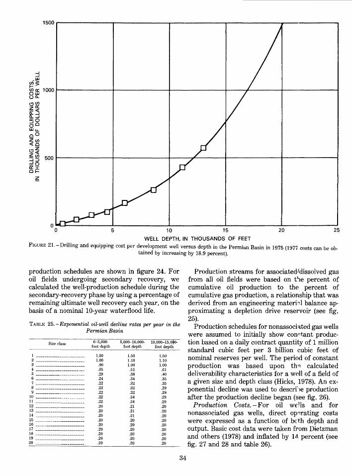
5 10 15 20 25

WELL DEPTH, IN THOUSANDS OF FEET

FIGURE 21.- Drilling and equipping cost per development well versus depth in the Permian Basin in 1975 (1977 costs can be ob­tained by increasing by 18.9 percent).

production schedules are shown in figure 24. For oil fields undergoing secondary recovery, we calculated the well-production schedule during the secondary-recovery phase by using a percentage of remaining ultimate well recovery each year, on the basis of a nominal 10-year waterflood life.

TABLE 25.-Exponential oil-well decline rates per year in the Permian Basin

Size class

1 -----------------------2 -----------------------3 -----------------------4 -----------------------5 -----------------------6 -----------------------7 -----------------------8 -----------------------9 -----------------------

10 -----------------------11 -----------------------12 -----------------------13 -----------------------14 -----------------------15 -----------------------16 -----------------------17 -----------------------18 -----------------------19 -----------------------20 -----------------------

0-5,000· foot depth

1.50 1.00

.90

.35

.29

.24

.22

.22

.22

.22

.22

.20

.20

.20

.20

.20

.20

.20

.20

.20

5,000-10,000- 10,000-15,0~0-foot depth foot depth

1.50 1.50 1.10 1.10 1.00 1.00

.51 .61

.38 .40

.34 .35

.32 .35

.32 .29

.32 .29

.24 .29

.24 .29

.21 .20

.21 .20

.21 .20

.20 .20

.20 .20

.20 .20

.20 .20

.20 .20

.20 .20

34

Production streams for associated/dissolved gas from all oil fields were based on t'-:te percent of cumulative oil production to the percent of cumulative gas production, a relationship that was derived from an engineering materi~.l balance ap­proximating a depletion drive reservoir (see fig. 25).

Production schedules for nonassoci::tted gas wells were assumed to initially show con~tant produc­tion based on a daily contract quantity of 1 million standard cubic feet per 3 billion cubic feet of nominal reserves per well. The period of constant production was based upon th~ calculated deliverability characteristics for a well of a field of a given size and depth class (Hicks, 1978). An ex­ponential decline was used to descri'-le production after the production decline began (see fig. 26).

Production Costs. -For oil wells and for nonassociated gas wells, direct op~rating costs were expressed as a function of beth depth and output. Basic cost data were taken f11 om Dietzman and others (1978) and inflated by 14 percent (see fig. 27 and 28 and table 26).

2000 en a: <l: ....J ....J 0 Q Ll.. 0 en c 1500 z <l: en ::J 0 J: ~

~ w' ....J

1000 0 J:

>-a: Q

~ z w ~ a.. 0 500 ....J w > w Q

Ll.. 0 ~ en 0 u

10 15 20

WELL DEPTH, IN THOUSANDS OF FEET

FIGURE 22. -Cost of development of dry hole versus depth in the Permian Basin in 1975 (1977 costs can be obtained by increasing by 18.9 percent).

TABLE 26.-A nnua.l direct operating expenses for non-associa.ted gas wells ·in the Perm·ian Basin in 1977 dollars

Size class 0-5,000- 5,000-10,000- 10,000-15,000- More than foot depth foot depth foot depth 15,000-foot depth

1-4 $3,600 $4,200 $5,800 $8,800 5 3,600 4,300 5,900 8,800 6 3,600 4,300 5,900 8,900 7 3,600 4,300 5,900 8,900 8 3,600 4,300 6,000 8,900 9 3,600 4,300 6,100 9,000

10 3,600 4,400 6,200 9,100 11 3,700 4,400 6,300 9,400 12 3,700 4,500 6,600 9,800 13 3,800 4,600 7,000 10,100 14 3,800 4,800 7,400 10,700 15 4,000 5,100 8,000 11,300 16 4,100 5,500 8,600 12,000 17 4,300 6,800 9,500 13,000 18 4,500 7,000 10,500 13,800 19 4,500 7,000 10,500 13,800 20 4,500 7,000 10,500 13,800

Indirect operating expenses include general and administrative overhead costs and certain proper­ty taxes. These costs are expressed on a per unit output basis and were set as $0.229 per barrel of oil and $0.0435 per 1,000 cubic feet of gas.

35

We calculated recovery per well for each price and return by accumulating annual production and assuming that production stops when the economic limit rate is reached. The economic limit if reached when the sum of operating costs and production­related taxes exceeds the operator's reveT}Ue.

ASSUMPTIONS FOR PRESENT VALUE CALCULATIONS

The following assumptions were used in the calculations of present values:

(1) A 5-year limit on the carryover of hsses for income tax purposes.

(2) Operators' working interest was 87.5 percent.

(3) State, county, and school property taxes and wellhead severance taxes are rollo.d into a royalty type tax of 6.4 percent of gross in­come for oil and 9.3 percent of gross in­come for gas.

(4) Federal income tax rate was 48 percent. (5) Depreciation method was unit of production

method.

100-----------------r----------------~---------------r----------------,

..J

..J w 75 ~

·ffi t;;a.. o(J) Ua: t-< zj wo ~CI 50 a.. - u. ~0 W(J) wCI (J)Z <t:< w(J) ..J:::::>

0 I I- 25 ~

4 8 12 16

WELL DEPTH, IN THOUSANDS OF FEET

FIGURE 23.- Lease equipment cost per well versus depth for primary oil production in the Permian Basin in 1976 (1977 costs can be obtained by increasing by 9.0 percent).

(6) Cost depletion was applied when determin­ing taxable income.

(7) Costs were based on mid-1977 prices, and the entire analysis assumed constant 1977 dollars.

(8) 70 percent of drilling costs for successful development wells along with dry-hole costs were expensed, and the remaining field-development costs were capitalized.

(9) Natural-gas prices were tied to the price of oil on a Btu basis.

ESTIMATED MARGINAL COST FUNCTIONS FOR UNDISCOVERED RECOVERABLE OIL AND GAS

RESOURCES IN THE PERMIAN BASIN

Economic analysis of the exploration process begins with the relationship between incremental units of exploration effort and the number and size

36

of fields discovered as a consequence of these units of effort.

The portion of the resource base that is physical­ly discoverable is restricted by the state-of-the-art of exploration technology. That portion always represents less than 100 percent of the un­discovered fields that may actually exist. Within this "effective upper limit" of a region's discoverable oil and gas, we expect the amounts found per unit effort to decrease as cumulative ex­ploration increases. However, a technical breakthrough in exploration can change the upper limit of what is discoverable and can increase the amounts discovered per unit of effort.

Given a discovery, the analysis shifts to the func­tion that describes physical relationships involved 1n the recovery of in-place resource~ .. Again the

...J

...J w ~

60

50

'a: 40 Zw oa.. i=CJ) u...J ::>w oa:: ~~ a.. al 30 ...JU. 60 ...JCJ) <(0 ::>Z z<( ZCJ) <(::> ~ 20 I-

~

10

5 10 15 20 25 30 35

TIME, IN YEARS

FIGURE 24.- Oil-production-decline curves for primary recovery at 7,200 feet in the Permian Basin.

state-of-the-art in production technology places an upper limit on the portion of oil and gas that can be physically recovered and produced. Even when the analysis includes future tertiary-recovery technology, less than 100 percent of the oil and gas in place is recovered.

In "Permian Basin Undiscovered Resources Ap­praisal," we discussed in detail subjective ap­praisals of the undiscovered oil and gas in place in the Permian Basin. In "The Discovery-Process Model," we described exploration and provided direct estimates of the number of fields that might be discovered with incremental units of ex-

ploratory effort. Estimates of what is recoverable from these future "discoveries" were th~n deter­mined by using the field-development information, production-decline curves, and cost data described in "Engineering and Cost Analysis for Future Fields."

37

The Permian Basin resource estimates and the discovery-process model were prep11red by separate task groups working concurrently, rather than sequentially. As a consequence, worl· remains' to be done in integrating more fully the Fubjective resource estimates and the historic discovery data projected by the discovery-process model.

>­a:

100

~ 80 0 u w a: (/) <( (!)

~ 60 <( ~

~ ::l

0 w 1-~ 40 CL X w u. 0 1-z w ~ 20 w c..

20 40 60 80 100

PERCENT OF EXPECTED ULTIMATE OIL RECOVERY

FIGURE 25.- Percent of expected ultimate gas recovery as a function of percent of expected ultimate oil recovery in the Permian Basin.

METHODOLOGY

This section is concerned with estimates of marginal cost functions for undiscovered recoverable oil and gas resources in the Permian Basin. We constructed the marginal cost curves by using the methods described in "The Discovery­Process Model" and "Engineering and Cost Analysis for Future Fields" and considering a return on investment and market prices of oil and gas.

The return and price considerations assume that i~cremental units of exploration, development, and production effort will not take place unless the ex­pected revenues received for eventual production sufficiently cover the incremental costs, including a normal rate of return on investment. The costs per

38

barrel of oil or per 1, 000 cubic feet of gas discovered, developed, and produced in the Per­mian Basin increase as additional units of effort in­crease. The marginal cost functions p:--esented here show how much of the theoretically di"coverable oil and gas, identified in "Permian Basin Un­discovered Resource Appraisal" and "The Discovery-Process Model," would be classified as recoverable at alternative prices and rates of return.

The output of the discovery-proces" model for a given increment of exploration is a frequency distribution of the expected number cf fields found for a particular size and depth catego:--y, where the size is expressed in BOE. To estimate the mar­ginal costs of finding and developing these un­discovered fields, the fields must be cr.tegorized as:

500

400 a: <( w >-

za:: ow -0.. ~~ uw 300 =>w gu. a::u O..iij (/):::> <(U c.9u.. ...Jo <((/) 200 :::>z zo z-<C:::l ~ ~

100

5 10 15 20 25 30

TIME, IN YEARS

FIGURE 26.- Nonassociated gas-well-production curve for a class-13 field in the depth bracket of 0-5,000 feet in the Permian Basin.

(1) crude oil and associated-dissolved gas and (2) nonassociated gas. The deposits in the "crude oil and associated-dissolved gas" category are then classified as: (1) technically susceptible to primary­recovery techniques alone, and (2) susceptible to both primary and secondary techniques. These categories are necessary for a more accurate iden­tification of the appropriate production processes and their related costs.

The economic analysis of the deposit is a stand­ard application of discounted cash flows (DCF). The net after-tax cash flow for a representative producing well is calculated and then discounted at various rates of return. The cash flows are ob­tained by subtracting operating costs, capital costs, and taxes from product revenues. If the calculations indicate that the DCF at an assumed

price level and rate of return is negative, that deposit is considered uneconomic and will not be produced.

The model can be applied in a straig'ltforward manner to determine which deposits will be pro­duced after discovery and how much oil and gas will be recovered under specific price and cost con­ditions. Determining how many additional ex­ploratory wells will be drilled is more dircult. The dynamics of the exploration process are not well understood, and probably no model can simulate actual practice realistically. However, it is possible to assume classical economic behavior unier condi­tions of perfect knowledge. Then, the number of exploratory wells drilled can be determined on the basis of the present value of future exploration cost being equivalent to the present value o:f develop-

39

15~----------------------~-----------------------,------------------------,

.....J

.....J w ~

(J)C::: 1-W 10 (/)0..

0(/) ua: (,9<( z.....J _.....J 1-0 <x:o a: LULl. c..o 0(/) .....JCI <z :::::>c:x: Z(J) z:::::> 5 <X:O

:I: I-

~

oo~----------------------~5~----------------------~10----------------------~15

WELL DEPTH, IN THOUSANDS OF FEET

FIGURE 27.-Annual direct operating cost per producing oil well versus depth for primary recovery in the Permian Basin in 1976 (1977 costs can be obtained by increasing by 14 percent).

ment (exclusive of exploration cost). In other words, the positive surplus of present value ob­tained through developing the various fields must eventually provide a cash flow adequate to pay for the number of exploratory wells drilled. Recogniz­ing the narrowness of these assumptions, the study group estimated the number of exploratory wells that could be drilled (in increments of 1,000 wells) until the incremental cost of drilling exploratory wells was equal to or greater than the present value of the developed deposits discovered by the last 1,000 exploratory-well increment. This point varied with the price and rate of return assumed.

SUMMARY OF RESULTS

Table 27 provides estimates of the oil and gas resources that could be found and produced from

40

the Permian Basin as a function of J: rice, finding cost, and production cost. The prices, rates of return, and number of exploratory wells that would be justified under the assumptions made are indicated. If the price is assumed to be $40 per BOE, the economically recoverable oil equivalent attains a maximum of 4. 7 billion BOY: at a 5 per­cent rate of return, 4.3 billion BOE at a 15 percent rate of return, and 3.9 billion BOE at a 25 percent rate of return. These quantities can b~ compared with the 38.2 billion BOE already discovered in the Permian Basin by the end of 1974.

Between 30,000 (at 25 percent rate of return) and 48,000 (at 5 percent rate of return) exploratory wells were estimated to be economic~.lly viable at the $40 price level. Figure 29 shows how the ex­ploratory effort varies as price and rG'.te of return

50~--------------------~----------------------,----------------------,

40 ....I ....J w ~

en a: 1-W (1.)0.. 0(/) uc:: 30 (.!)<( z....l _....J 1-0 <(C c:: wu. a..O 0(/) ....JC <Cz ::::><( Z(f.)

20

z::::> <CO

I I-

~

10

ooL------------------------4~----------------------....Js~--------------------~,2

WELL DEPTH, IN THOUSANDS OF FEET

FIGURE 28. -Annual direct operating cost per producing oil well versus depth for secondary recovery in the Permian B<~.sin in 1975 (1977 costs can be obtained by increasing by 14 percent).

vary. This can be compared with the slightly more than 30,000 exploratory wells which were drilled in the Permian Basin through December 31, 1974, in which approximately 10 times more BOE were discovered than the BOE projected for the next 30,000-48,000 wells.

At $15 a barrel and a 15 percent rate of return, only 12,000 exploratory wells would be drilled and 2.3 billion BOE reserves added. The model can be used to answer two questions: (1) what price and rate of return are required to stimulate a certain level of exploration to find a given amount of oil and gas in BOE's?; or, (2) what amount of oil and gas can be anticipated from the Permian Basin at the present or some future price and rate of return?

The output of the model can be examined m

41

terms of associated-dissolved gas, non~.ssociated gas, and oil resulting from various price levels and rates of return. The graphs shown in figures 30-32 reveal the declining size of the targets discovered as a result of additional exploratory effort. As the marginal cost curves turn sharply upward, oil- and gas-reserve additions to be gained at costs of $10 to $25 per barrel are considerably greater than those at $25 to $40 per barrel.

Another interesting result shown in the analysis is the dominance of nonassociated gas in the re­maining resources in the Permian B~sin. This dominance is true under all price and rate-of-re­turn assumptions. When nonassociated gas is added to the associated-dissolved gas:, crude oil represents only about one-quarter of the future potential.

TABLE 27.-PotenNal recoverable oil and ga.s resources from. fu.tu.re d·iscoveri.es in the Permian Basin as a function of output price, ma·rginal finding cost, marginal production cost, exploratory wells, and return on investment (ROI)

[BOE, barrels of oil equivalent; Tcf, trillions of standard cubic feet of natpral gas]

CUMULATIVE POTENTIAL RESOURCES

Output Cumulative ROI exploration a Marginal oosts2 Associated gas Nonassociated gas

price (percent) wells' ($/BOE)

(in thousands) Finding Production OilBOE Tcf BOE Tcf BOE Total BOE ($/BOE) ($/BOE) (in billions) (in billions) (in billions) (in billions)

10 -------- 5 10 $ 2.64 $ 7.36 0.489 1.371 0.260 6.803 1.291 2.040 15 5 1.67 8.33 .264 .750 .142 4.234 .803 1.209 25 2 1.26 8.74 .108 .304 .058 1.948 .370 .536

15 -------- 5 19 4.58 10.42 .813 2.273 .431 9.384 1.781 3.025 15 12 3.00 12.00 .578 1.614 .306 7.559 1.434 2.318 25 8 2.15 12.85 .417 1.164 .221 5.982 1.135 1.773

;!:>-1:\:1 20 -------- 5 26 6.40 13.60 1.013 2.822 .535 10.654 2.022 3.570

15 18 4.30 15.'/0 .792 2.205 .419 9.170 1.740 2.951 25 12 2.97 17.03 .582 1.621 .308 7.586 1.436 2.326

25 -------- 5 33 8.49 16.51 1.178 3.276 .622 11.610 2.203 4.003 15 24 5.79 19.21 .965 2.684 .509 10.332 1.961 3.435 25 17 4.03 20.97 .763 2.121 .393 8.954 1.699 2.865

30 5 38 10.30 19.70 1.278 3.536 .670 12.220 2.319 4.268 15 29 7.14 22.86 1.094 3.014 .572 11.110 2.108 3.774 25 22 5.19 24.81 .918 2.547 .483 9.996 1.897 3.298

35 -------- 5 43 12.27 22.63 1.366 3.788 .719 12.741 2.418 4.503 15 34 8.65 26.35 1.202 3.334 .632 11.803 2.240 4.075 25 26 6.19 28.81 1.024 2.839 .539 10.712 2.033 3.596

40 -------- 5 48 14.59 25.41 1.488 4.006 .760 13.162 2.498 4.706 15 38 10.05 29.95 1.284 3.557 .675 12.253 2.325 4.284 25 30 7.31 32.69 1.119 3.100 .588 11.294 2.143 3.850

1 Exploratory wells assumed to be drilled since December 31, 1974. The stopping rule for exploratory wells drilled does not take into account the tax benefit of charging the cost of exploratory wells against current income. Therefore, these figures overestimate the effective cost of exploratory drilling.

2 At the margin, the sum of the marginal finding cost and the marginal production cost is equal to the output price (column 1).

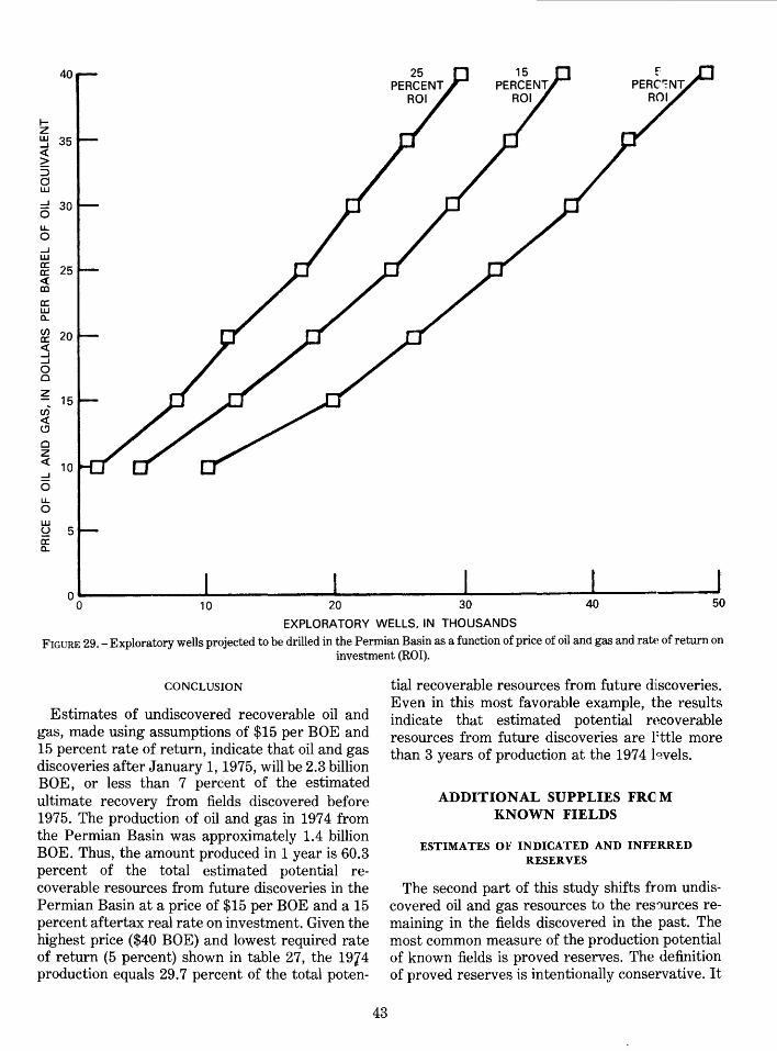
40

1-z w 35 ....J <( > 5 0 w ....J 30 6 u.. 0 ....J w (I:

25 (I: <( CXl

0:: w Q..

(/) 20 0:: <( ....J ....J 0 0

~ 15 u) <( (.9

Cl z <(

10 ....J

6 u.. 0 w ~ 5 0:: Q..

0 oL--------------1•o--------------2~o---------------3~o--------------4~o------------~5o

EXPLORATORY WELLS, IN THOUSANDS

FIGURE 29.- Exploratory wells projected to be drilled in the Permian Basin as a function of price of oil an<1 gas and rau• of return on investment (ROI).

CONCLUSION

Estimates of undiscovered recoverable oil and gas, made using assumptions of $15 per BOE and 15 percent rate of return, indicate that oil and gas discoveries after January 1, 1975, will be 2.3 billion BOE, or less than 7 percent of the estimated ultimate recovery from fields discovered before 1975. The production of oil and gas in 1974 from the Permian Basin was approximately 1.4 billion BOE. Thus, the amount produced in 1 year is 60.3 percent of the total estimated potential re­coverable resources from future discoveries in the Permian Basin at a price of $15 per BOE and a 15 percent aftertax real rate on investment. Given the highest price ($40 BOE) and lowest required rate of return (5 percent) shown in table 27, the 1944 production equals 29.7 percent of the total poten-

43

tial recoverable resources from future discoveries. Even in this most favorable example, the results indicate that estimated potential recoverable resources from future discoveries are l;ttle more than 3 years of production at the 1974 l~vels.

ADDITIONAL SUPPLIES FR<J M KNOWN FIELDS

ESTIMATES OF INDICATED AND INF:ERRED RESERVES

The second part of this study shifts from undis­covered oil and gas resources to the res'lurces re­maining in the fields discovered in the past. The most common measure of the production potential of known fields is proved reserves. The definition of proved reserves is intentionally conservative. It

1-z w ....J

~ ::::> d w ....J

5 u.. 0 ....J w a: a: <( co a: w a.. (/) a: <{ ....J ....J 0 0

~ t-' (/)

0 u ....J <( z (.9 a: <{ ~

15

10

5

NONASSOCIATED GAS

a~--------------._--------------~--------------~--------------~~------------~ 0 2 3 4 5

OIL EQUIVALENT, IN BILLIONS OF BARRELS FIGURE 30.- Marginal cost of recoverable oil and gas resources from undiscovered deposits in the Permian Basin- 5 percent dis­

counted cash-flow rate of return.

reflects the measurements, estimates, and historical production data for the field and provides a projection that is unlikely to overstate what can be produced in the future at current prices and technology.

The proved reserves of the Permian Basin reported by the industry as of December 31, 1976, were: 5.5 billion barrels of oil and 18.2 trillion cubic feet of natural gas, 6 as compared with past produc~ tion from the Permian Basin of 18.6 billion barrels of oil and 55.8 trillion cubic feet of natural gas. A judgment can be made concerning how much oil

6 These figures represent the sum of proved reserves reported by the American Petroleum Institute and the American Gas Association for the Southeast New Mex­ico District and Texas Railroad Commission Districts, 7C, 8, and 8A. The four dis­tricts, although not 1dentical to the Permian Basin as defined in this report, closely approximate it and are considered identical for the purpose of counting reserves and original oil in place.

and gas was originally in place in the parts of known fields that provided this past production and that contain the remaining proved reserves. These amounts are approximately 90.4 billion bar­rels of oil and 108.4 trillion cubic feet of natural gas. The combination of past proiuction and proved reserves indicates that 26.0 percent of the oil will ultimately be recovered in the Permian Basin.

As additional production experience is gained and as more development and extension wells are drilled in known fields, additional quantities of oil and gas may be projected with sufficiert confidence to include these quantities in the proved category. Subsequent production must be subtracted from e~rlier proved estimates, and new information may cause upward or downward revisions in previous

44

40

~35 z w ....J

~ 5 030 w ....J

0 LL 0 ....J 25 w a: a: <( CD

a: ~20 (/) a: :3 ....J 0 0 15 ~ ~' (/)

0 u <i! 10

~ (.!) a: <( :E

5

TOTAL

2 3 4 5

OIL EQUIVALENT, IN BILLIONS OF BARRELS FIGURE 31.~Marginal cost of recoverable oil and gas resources from undiscovered deposits in the Permian Basin-15 percent dis­

counted cash-flow rate of return.

estimates. History indicates also that the recovery factor does not remain constant over time because new secondary projects are introduced into fields and economic conditions change. As a conse­quence, the estimate of ultimate recovery, as well as perceptions of the amount of oil and gas origi­nally in place, changes gradually over time.

INDICATED RESERVES

The initial step in accounting for the known oil and gas resources of the Permian Basin is, there­fore, to estimate how much oil and gas may be pro­duced from known fields, in addition to that in­cluded in proved reserves. Included in the first of these additional amounts are the quantities of oil expected to be recovered from projects that will

45

improve recovery in active fields- projet~ts where secondary recovery operations have begun, but are too new to evaluate; and proposed projects, which must be evaluated according to experien~e gained in other fields. According to the American Petro­leum Institute (American Gas Association and others, 1977, table 1) these "indicated additional reserves" amounted to 1. 6 billion barrels of recov­erable oil as of December 31, 1976.

INFERRED RESERVES

The combination of proved reserves plus any in­dicated additional r~serves does not full;T account for the potential of the known fields. The dis­covered reserves of oil and gas also include in­ferred reserves, which are hydrocarboTls whose

40

1- 35 z w ....J

~ 5 d 30 w ....J

6 LL 0 ....J 25 w a: a: <( Ill

(/) a: :5 ....J 0 Q 15 z r: (/)

0 u ~ 10 ~ (.!) a: <( ~

TOTAL

ooL-------------L--------------L2--------------~3~------------~4~--~------~5

OIL EQUIVALENT, IN BILLIONS OF BARRELS FIGURE 32.-Marginal cost of recoverable oil and gas resources from undiscovered deposits in the Permian Basin-25 percent dis­

counted cash-flow rate of return.

quantity cannot be precisely determined. Never­theless, this additional oil and gas probably will be recovered eventually, and its recovery will notre­quire the exploratory drilling needed for a new field discovery.

For all fields discovered in a given year, the American Gas Association (AGA), the American Petroleum Institute (API) and the Canadian Petro­leum Association (CPA) have published through 1978 (American Gas Association and others, 1967-79) annual estimates of ultimate recovery. Changes in estimates of the quantity in place plus the recoverable quantities (proved reserves plus production) provide some basis for estimating the degree to which reserve and recovery figures may

46

change over time for individual fielc1 ~, an entire basin, or the United States as a whol~. Estimates of ultimate recovery eventually stabilize for mature fields and become good proje~tions of the actual recoverable quantity, if we asEume that no changes in price or technology take place.

GENERAL OUTLINE OF DATA AND METHODS

Proved reserves of crude oil and natural gas are defined by the API and AGA. These d~finitions in­clude only the part of the oil and gas r~~source base that is known to be technically and economically producible. Because the estimate of proved reserves in a field depends on the degree of

development and production in each field, the esti­mates are updated each year. On the average, esti­mates of ultimate recovery (past production plus proved reserves) increase with time; the changes in estimates are due to extensions, revisions, and new reservoir discoveries in old fields (referred to as "new pools" in subsequent discussion). Extensions and new pools are proved reserve additions war­ranted by increases in the perceived physical di­mensions of the field as a result of additional drill­ing. Revisions are all other changes (either positive or negative). Generally, estimates of a field's ultimate production grow more rapidly in the first few years after discovery; most fields are well­defined after 6 years of development and pro­duction.

Data on ultimate recovery can be used to esti­mate how much oil will actually be produced from fields that are not yet fully developed, if we assume that the estimates of their ultimate recovery grow in the same way that such estimates grew in the past. Briefly, an estimate of ultimate recovery for each year of age is made as the fields pass through that year of age. For example, the amount of growth as the fields advance from their fifteenth to their sixteenth year would be indicated by the changes in estimates for December 31, 1966, and December 31, 1967, for fields discovered in 1951. The percentage changes between successive estimates for all years for which data are available can then be calculated. The mean percentage change is the average growth that can be expected as fields age from their fifteenth to their sixteenth year.

Such expected growth was calculated for each year. The estimated ultimate recovery for fields discovered in a given year was multiplied by the growth factors for each year beyond the age of the fields. The same method of analysis was also ap­plied to original oil in place and to recoverable natural gas for the Permian Basin. Results are presented in tables 28 and 29.

METHOD OF ANAL YSlS

Let Qe(u, v) be the estimate of ultimate recovery made at the end of year v for all fields discovered during the year u. Let Q(u) be the actual, but un­known, amount of oil discovered in year u. We assume that:

Qe(u, v)=Q(u)f(v-u)+Q(u)E(u, v) (1)

where f(v-u) is a fraction which increases to 1.0 as the age of the fields, v- u, increases to infinity.

TABLE 28.-Growth 'in estimates of original oil "in placefor the Permian Basin

[In this table, Permian Basin comprises Southeastern New Mexico and Texas Railroad Commission Districts 7C, 8, and SA]

Di~~::ry Estimate Age of estimate 1/ftt) Corrected 12/31/76 in yrs e~t.imate

(billion bbl.) (t) (billion bbl.)

1975 ------ 0.0472 0.5 5.84 0.2755 1974 .0416 1.5 2.89 .1201 1973 ------ .1610 2.5 1.95 .3142 1972 .0997 3.5 1.76 .1753 1971 .0857 4.5 1.58 .1353 1970 .2359 5.5 1.42 .3347 1969 .2511 6.5 1.36 .3409 1968 .1041 7.5 1.32 .1372 1967 ------ .1893 8.5 1.29 .2446 1966 .6271 9.5 1.27 .7939 1965 ------ .5114 10.5 1.25 .6387 1964 .4189 11.5 1.22 .5109 1963 .2555 12.5 1.23 .3136 1962 .7279 13.5 1.23 .8932 1961 .3888 14.5 1.22 .4735 1960 .7398 15.5 1.21 .8936 1959 ------ .6283 16.5 1.21 .7595 1958 .4246 17.5 1.20 .5105 1957 1.6167 18.5 1.15 1.8528 1956 ------ 1.5509 19.5 1.14 1.7676 1955 1.0706 20.5 1.14 1.2171 1954 ------ 2.7785 21.5 1.12 3.1193 1953 2.8443 22.5 1.11 3.1439 1952 1.0497 23.5 1.10 1.1542 1951 1.2816 24.5 1.07 1.3707 1950 2.4700 25.5 1.04 2.5806 1949 ------ 12.4150 26.5 1.01 12.5650 1948 4.0569 27.5 1.04 4.2146 1947 2.0158 28.5 1.03 2.0856 1946 .8728 29.5 1.03 .8975 1945 ------ 3.5591 30.5 1,05 :3.7296 1944 2.4933 31.5 1.02 2.5443 1943 1.4396 32.5 L02 1.4716 1942 .8482 33.5 1.04 .8818 1941 2.2130 34.5 1.02 2.2491 1940 1.9322 35.5 L02 1.9704 1939 1.4757 36.5 L01 1.4868 1938 .8560 37.5 L02 .8733 1937 ------ .7615 38.5 L02 .7766 1936 6.8011 39.5 1.02 1).9313 1935 2.2127 40.5 L02 2.2520 1934 2.6043 4L5 L01 :l.6344 1933 .2241 42.5 1.01 .2266 1932 .5565 43.5 1,02 .5695 1931 ------ .0082 44.5 L03 .0084 1930 3.3113 45.5 1.01 :1.3519 1929 ------ 5.1144 46.5 L01 ii.1639 1928 1.4529 47.5 1.00 1.4575 1927 .6538 48.5 1.00 .6558 1926 8.5027 49.5 1.00 8.5027 1925 2.0742 50.5 1.00 ::.0742 1924 .1249 5L5 1.00 .1249 1923 .5842 52.5 1.00 .5842 1922 0 53.5 1.00 0 1921 .1658 54.5 1.00 .1658 1920 ------ 0 55.5 0 Pre-1920 (I 0

Total 89.9300 94.5200

The error term, Q(u)E(u,v), is assumed to be pro­portional to Q(u). Taking logarithms gives:

lnQe(u, v)= lnQ(u) + ln(f(v- u)+E(u, v)).

We now fix u and regard both sides as functions of v only and ignore the error term, E(u,v).

Taking the difference betwen successive esti­mates of the amount of oil or gas discovered in a year u gives equation (2):

lnQe(U,V+ 1)-lnQe(u, v)=ln.f{v+ 1-u)-ln./{v·-u) (2).

47

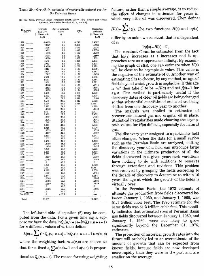
TABLE 29.- Gro·wth in est·imates of recoverable natu.ral gas for the Perm·ian Basin

[In this table, Permian Basin comprises Southeastern New Mexico and Texas Railroad Commission Districts 7C, 8, and SA]

Di~J>i'rery Estimate Age of estimate Corrected 12/31/76 in yrs 1/j{t) estimate

(trillion cubic (t) (trillion cubic feet) feet)

1976 0.0965 0.5 4.748 0.4582 1975 .2377 1.5 2.311 .5493 1974 .3787 2.5 1.673 .6336 1973 .9057 3.5 1.499 1.3578 1972 .4966 4.5 1.462 .7260 1971 .5044 5.5 1.360 .6860 1970 .6070 6.5 1.326 .8051 1969 1.587 7.5 1.326 2.105 1968 1.962 8.5 1.250 2.452 1967 0.9316 9.5 1.201 1.119 1966 1.347 10.5 1.195 1.6091 1965 1.004 11.5 1.176 1.181 1964 .7197 12.5 1.177 .8470 1963 5.951 13.5 1.186 7.060 1962 2.653 14.5 1.189 3.154 1961 1.301 15.5 1.238 1.611 1960 .8093 16.5 1.176 .9514 1959 .2894 17.5 1.1027 .3191 1958 .8278 18.5 1.134 .9386 1957 1.466 19.5 1.085 1.590 1956 1.371 20.5 1.063 1.458 1955 .6345 21.5 1.018 .6460 1954 2.596 22.5 1.012 2.628 1953 1.574 23.5 1.014 1.596 1952 2.815 24.5 1 2.815 1951 .4043 25.5 1 .4043 1950 2.77 26.5 1 2.777 1949 2.452 27.5 1 2.452 1948 .8001 28.5 1 .8001 1947 .8041 29.5 1 .8041 1946 .7491 30.5 1 .7491 1945 3.048 31.5 1 3.048 1944 2.016 32.5 1 2.016 1943 .4739 33.5 1 .4738 1942 .3197 34.5 1 .3197 1941 1.241 35.5 1 1.241 1940 .2037 36.5 1 .2037 1939 1.432 37.5 1 1.432 1938 .3360 38.5 1 .3360 1937 .1426 39.5 1 .1426 1936 3.295 40.5 1 3.295 1935 1.435 41.5 1 1.435 1934 2.257 42.5 1 2.257 1933 .0497 43.5 1 .0497 1932 .1268 44.5 1 .1268 1931 .0 45.5 1 .0 1930 2.692 46.5 1 2.692 1929 10.55 47.5 1 10.55 1928 1.075 48.5 1 1.075 1927 .1751 49.5 1 .1751 1926 1.284 50.5 1.284 1925 .2503 51.5 .2503 1924 .2806 52.5 .2806 1923 .1989 53.5 . 1989 1922 .0 54.5 .0 1921 .0026 55.5 .0026 1920 .0 56.5 .0 Pre-1920 .0 a:57.5

Total 73.937 81.167

The left-hand side of equation (2) may be com­puted from the data. For a given time lag s, sup­pose we have the data lnQe(u,u+s)-lnQe(u,u+s-1) for n different values of u, then define:

h(s)= .E (lnQe(u, u+s)-lnQe(u, u+s-1)*a(u, s) u

where the weighting factors a(u,s) are chosen so

that for a fixed s, _Ea(u,s)= 1 and a(u,s) is propor-u

tional to Qe(u,u+s). The reason for using weighting

factors, rather than a simple average, is to reduce the effect of changes in estimates for years in which very little oil was discovered. Then define:

s

H(s)= .Eh(i). The two functions H(s) and lnf(s) i=l

differ by an unknown constant, that is independent of s:

ln.f{s)=H(s)+C. The constant C can be estimated from the fact

that ln.f{s) increases as s increases and it ap­proaches zero as s approaches infinity. By examin­ing the graph of H(s), one can esti1nate when H(s) will be close to its asymptotic valua.. This value is the negative of the estimate of C. Another way of estimating C is to choose, by any method, an age of fields beyond which growth is negligible. If this age is "a" then take C to be -H(a) and set.f{s)=1 for s ~a. This method is particularly useful if the discovery dates of older oil fields are being changed so that substantial quantities of crude oil are being shifted from one discovery year to another.

The analysis was applied to estimates of recoverable natural gas and original oil in place. Statistical irregularities made choo~ing the asymp­totic values for H(s) difficult, especially for natural gas.

The discovery year assigned to a particular field often changes. When the data for a small region such as the Permian Basin are an~.lyzed, shifting the discovery year of a field can introduce large variations in the ultimate production of all the fields discovered in a given year; such variations have nothing to do with additions to reserves through extensions and revisions. This problem was resolved by grouping the fields according to the decade of discovery to determjne to within 10 years the age at which the growtr of the fields is virtually over .

In the Permian Basin, the 1973 estimate of ultimate gas production from fields discovered be­tween January 1, 1950, and January 1, 1960, was 51.1 trillion cubic feet. The 1976 estimate for the same fields was 51.3 trillion cubic feet. This stabili­ty indicated that estimated sizes of Permian Basin gas fields discovered between January 1, 1950, and January 1, 1960, were not likely to grow significantly beyond the Decem'ler 31, 1976, estimates.

The projection of historical growth rates into the future will probably led to an overestimate of the amount of growth that can be expected from known fields, because fields are now developed more rapidly than they were in tr~ past and are smaller on the average.

48

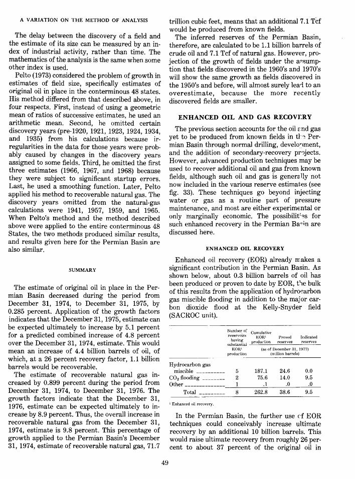
A VARIATION ON THE METHOD OF ANALYSIS

The delay between the discovery of a field and the estimate of its size can be measured by an in­dex of industrial activity, rather than time. The mathematics of the analysis is the same when some other index is used.

Pelto (1973) considered the problem of growth in estimates of field size, specifically estimates of original oil in place in the conterminous 48 states. His method differed from that described above, in four respects. First, instead of using a geometric mean of ratios of successive estimates, he used an arithmetic mean. Second, he omitted certain discovery years (pre-1920, 1921, 1923, 1924, 1934, and 1935) from his calculations because ir­regularities in the data for those years were prob­ably caused by changes in the discovery years assigned to some fields. Third, he omitted the first three estimates (1966, 1967, and 1968) because they were subject to significant startup errors. Last, he used a smoothing function. Later, Pelto applied his method to recoverable natural gas. The discovery years omitted from the natural-gas calculations were 1941, 1957, 1959, and 1965. When Pelto's method and the method described above were applied to the entire conterminous 48 States, the two methods produced similar results, and results given here for the Permian Basin are also similar.

SUMMARY

The estimate of original oil in place in the Per­mian Basin decreased during the period from December 31, 1974, to December 31, 1975, by 0.285 percent. Application of the growth factors indicates that the December 31, 1975, estimate can be expected ultimately to increase by 5.1 percent for a predicted combined increase of 4.8 percent over the December 31, 1974, estimate. This would mean an increase of 4.4 billion barrels of oil, of which, at a 26 percent recovery factor, 1.1 billion barrels would be recoverable.

The estimate of recoverable natural gas in­creased by 0.899 percent during the period from December 31, 1974, to December 31, 1976. The growth factors indicate that the December 31, 1976, estimate can be expected ultimately to in­crease by 8. 9 percent. Thus, the overall increase in recoverable natural gas from the December 31, 1974, estimate is 9.8 percent. This percentage of growth applied to the Permian Basin's December 31, 1974, estimate of recoverable natural gas, 71.7

49

trillion cubic feet, means that an additional 7.1 Tcf would be produced from known fields.

The inferred reserves of the Permian Basin, therefore, are calculated to be 1.1 billion barrels of crude oil and 7.1 Tcf of natural gas. However, pro­jection of the growth of fields under the a~sump­tion that fields discovered in the 1960's and 1970's will show the same growth as fields discovered in the 1950's and before, will almost surely lea-l to an overestimate, because the more recently discovered fields are smaller.

ENHANCED OIL AND GAS RECOVJ:RY

The previous section accounts for the oil r.nd gas yet to be produced from known fields in tl'~ Per­mian Basin through normal drilling, develo~ment, and the addition of secondary-recovery pr')jects. However, advanced production techniques may be used to recover additional oil and gas from known fields, although such oil and gas is gener21ly not now included in the various reserve estimates (see fig. 33). These techniques go beyond injecting water or gas as a routine part of pressure maintenance, and most are either experimental or only marginally economic. The possibilif~s for such enhanced recovery in the Permian Ba"'in are discussed here.

ENHANCED OIL RECOVERY

Enhanced oil recovery (EOR) already makes a significant contribution in the Permian Basin. As shown below, about 0.3 billion barrels of oil has been produced or proven to date by EOR, t'le bulk of this results from the application of hydro~arbon gas miscible flooding in addition to the major car­bon dioxide flood at the Kelly-Snyder field (SACROC unit).

Number of Cumulative reservoirs EORI Proved Indicated

having production reserves reserves substantial ----'-------------

EOR1 (as of December 31, 1977) production (million barrels)

Hydrocarbon gas miscible ---------- 5 187.1 24.6 0.0

C02

flooding ________ 2 75.6 14.0 9.5 Other-------------- 1 .1 .0 .0

Total --------- 8 262.8 38.6 9.5

1 Enhanced oil recovery.

In the Permian Basin, the further use C'f EOR techniques could conceivably increase ultimate recovery by an additional 10 billion barrels. This would raise ultimate recovery from roughly 26 per­cent to about 37 percent of the original oil in

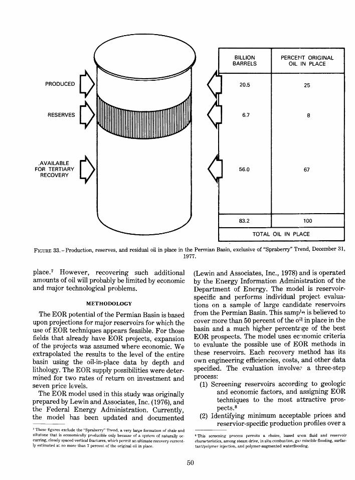
PRODUCED

RESERVES 1:/

.AVAILABLE 1:/ FOR TERTIARY

RECOVERY

BILLION BARRELS

20.5

6.7

56.0

83.2

PERCEriT ORIGINAL OIL IN PLACE

25

8

67

100

TOTAL OIL IN PLACE

FIGURE 33.-Production, reserves, and residual oil in place in the Permian Basin, exclusive of "Spraberry" Trend, December 31, 1977.

place. 7 However, recovering such additional amounts of oil will probably be limited by economic and major technological problems.

METHODOLOGY

The EOR potential of the Permian Basin is based upon projections for major reservoirs for which the use of EOR techniques appears feasible. For those fields that already have EOR projects, expansion of the projects was assumed where economic. We extrapolated the results to the level of the entire basin using the oil-in-place data by depth and lithology. The EOR supply possibilities were deter­mined for two rates of return on investment and seven price ltvels.

The EOR model used in this study was originally prepared by Lewin and Associates, Inc. (1976), and the Federal Energy Administration. Currently, the model has been updated and documented

7 These figures exclude the "Spraberry" Trend, a very large formation of shale and silts~one that is economically producible only because of a system of naturally oc­curn~g, closely spaced vertical fractures, which permit an ultimate recovery current­ly estimated at no more than 7 percent of the original oil in place.

50

(Lewin and Associates, Inc., 1978) and is operated by the Energy Information Administration of the Department of Energy. The model is reservoir­specific and performs individual project evalua­tions on a sample of large candidate reservoirs from the Permian Basin. This sampl~ is believed to cover more than 50 percent of the o~l in place in the basin and a much higher percenU'.ge of the best EOR prospects. The model uses ec':lnomic criteria to evaluate the possible use of EOR methods in these reservoirs. Each recovery 1nethod has its own engineering efficiencies, costs, and other data specified. The evaluation involve;;- a three-step process:

(1) Screening reservoirs according to geologic and economic factors, and assigning EOR techniques to the most attractive pros­pects.8

(2) Identifying minimum acceptable prices and reservior-specific production profiles over a

8 This screening process permits a choice, based u"lon fluid and reservoir characteristics, among steam drive, in situ combustion, ga:' miscible flooding, surfac­tant/polymer injection, and polymer-augmented waterflooding.

period of time, on the basis of projected market prices and rates of return.

(3) Extrapolating production data to regional levels and accumulating reserves.

The study was conducted separately for sand­stone and carbonate reservoirs, which then were classified by reservoir depth. Ninety-six reservoirs were included in the sample studied. The distribu­tion of the reservoirs within these categories is given in table 30. The sample was extrapolated to obtain estimated values for the entire basin for both sandstone and carbonate formations and for various reservoir depths. The extrapolation factors used and the results obtained are shown below:

Reservoir type <5 000 ft 5•000- 10•000 > 10 000 ft ' ft '

Sandstone: Sample OOIP 1

, billion bbls ----------­Total OOIP, billion bbls -------------­Extrapolation factor ----------------

Carbonate: Sample OOIP, billion bbls -----------­Total OOIP, billion bbls -------------­Extrapolation factor ----------------

1 Original ore in place.

1.65 10.81

.153

25.17 32.50

.774

0.22 4.94 .0.40

.045

15.64 2.94 26.87 7.68

.582 .383

TABLE 30. -Classification of sample reservoirs selected for enhanced oil recovery in the Permian Basin

Technically feasible for EOR a

Sandstone ------------­Carbonate

Infeasible for EOR~---------

<5,000

No. OOIP 1

(109B) 2

2 1.65 34 19.88

5,000-10,000 ft > 10,000 ft

No. OOIP No. OOIP (109B) (109B)

2 0.22 29 14.31 2.44

5.29 1.33 10 .50

41 26.8 36 15.9 19 2.9

Sandstone ------------­Carbonate -------------Total ________________ · _ __:____:::.:..=.::.. _ ___::..__--=.:.::.::___.::.::...__.::::..::__

1 Original oil in place. 2 B, barrel. 3 Enhanced oil recovery.

The technology assumed was the best of the cur­rently tested and applied carbon dioxide processes. More specifically, the model includes assumptions that:

(1) Oil saturation is uniformly distributed within the part of the reservoir being developed at the time the project is initiated (this assumption may lead to an underestimate of drilling costs and, hence, an overestimate of recovery).

(2) The effective sweep efficiency for the carbon dioxide varies according to the perfor­mance of the waterflood previously used and the reservoir lithology (that is, car­bonate or sandstone); the carbon dioxide sweep efficiency used by the model is a

function of ultimate primary/secondary sweep, as follows:

00 sweep efficiency

[Percent of waterflood sweep]

Reservoir suitability 1

Good ---------------------Fair----------------------Poor ---------------------

Sandstone reservoirs

50 40 30

1 As determined by the National Petroleum Council (1976).

Carbonate reservoirs

45 40 35

(3) Residuql oil saturation in the swept zone after carbon dioxide flooding is 60 percent of the residual after waterflooding.

( 4) Residual oil saturation in the unswept zone remains unchanged.

(5) World oil prices remain at the mid-1977 level in constant dollar terms.

Potential EOR production ranges from zero pro­duction at $10 per barrel to 5.1 billion and 4.6 billion barrels at $40 per barrel for rates of return at 15 percent and 25 percent, respectively, as shown in table 31.

TABLE 31.-Enhanced oil recovery potential of the Permian Basin

[In billions of barrels; BOE, barrels of oil equivalent]

Output price 15 percent 25 percent ($/BOE) rate of return rate of return

10 ---------------- 0.0 0.0 15 ---------------- 1.34 .20 20 ---------------- 2.93 1.30 25 ---------------- 4.31 2.58 30 ---------------- 4.70 3.65 35 ---------------- 5.08 4.11 40 ---------------- 5.11 4.56

ENHANCED GAS RECOVERY

Conventional gas production ordinarily recovers· a large fraction of the original gas in place, 70 per­cent or more in the Permian Basin; the remaining gas is generally not an attractive target for enhanced gas recovery (EGR) techniques.

The usual targets for EGR, instead, are· discovered gas accumulations that have never been produced because conventional production methods are uneconomic. The gas in these fields is classified as a discovered subeconomic resource and is frequently designated "near-conventional" or "unconventional" gas, to indicate the subeconomic responsP to conventional production methods.

51

Within the Permian Basin, interest in EGR centers on the southern part, Sutton, Crockett,

____________ ___j__

31

PECOS

r---

' ,-~

"'' I "'-l I '"-,"- ~-.J TERRELL

3~~ EXPLANATION ,

l\t~\\jilijj!j:jjjjjjjjjjijj!j North a rea

~~~~South area

20

I I

20 I

UNITED I STATES

MEXIco

40 MILES I

40 KILOMETERS

KIMBLE

-l-1

VAL VERDE

_ _l__

---1 I I

! EDWARDS 1 L-_____ Lt_ __ _ REAL

I

FIGURE 34.-Areas of the Permian Basin for enhanced gas recovery.

and Schleicher Counties in Texas (see fig. 34). TABLE 32.-Enhanced gas recovery potential of the Permian

About 4,500 square miles of this subbasin may be Basin responsive to massive hydraulic fracturing (MHF) [In trillion cubic feet; BOE. barrels of oil equivalent]

at some future time under the economic conditions assumed in this study.

MHF now has advanced sufficiently to become standard production practice in many fields of low permeability. However, the economic and subeconomic resources of the area are difficult to identify separately. This report, therefore, assumes that all such resources are presently subeconomic and that exploiting this area will re­quire future technological advances.

EGR using MHF was analyzed at two rates of return and at a wide range of price levels (see table 32). The methodology was similar to that for EOR. The response ranges from 7.4 trillion cubic feet at $10 per BOE and 25 percent rate of return to 13.7 trillion cubic feet at $40 per BOE and either 15 or 25 percent rate of return.

52

Output price 15 percent 25 percent ($/BOE) rate of return rate of return

5 ---------------- 8.9 7.4 10 ---------------- 13.7 13.7 15 ---------------- 13.7 13.7 20 ---------------- 13.7 13.7 25 ---------------- 13.7 13.7 30 ---------------- 13.7 13.7 35 ---------------- 13.7 13.7 40 ---------------- 13.7 13.7

EXPANDED PRODUCTION FROM KNOWN FIELDS: AN APPRAISAL OF RESULTS

Although the undiscovered oil and gas resources of the Permian Basin have been discussed in "The Integrating Economic Model," the second part oJ! this study, which addresses future supply from

known fields and analyzes separate problems, re­quired different approaches. The statistical outputs given in "Estimates of Indicated and Inferred Reserves" and "Enhanced Oil and Gas Recovery" are less uniform in character than those in "Future Production of Undiscovered Oil and Gas from the Permian Basin," and, consequently, are difficult to aggregate. Therefore, a formal integrating model to show the potential for future recovery of oil and gas from known reservoirs has not been at­tempted.

Using one set of assumptions (such as $15 per BOE and 15 percent rate of return), we can itemize (see following table) the current outlook in the Per­mian Basin for recovering additional oil and gas from discovered fields. In a general way, this table provides a concept of the relative magnitude of future supply.

Reserves as of Oil Natural gas December 31, 1976 (billion barrels) (trillion cubic feet)

Proved -------------- 5.5 18.2 Indicated additional ____ 1.6 Inferred ------------- 1.1 7.1 From enhanced-recovery

techniques ---------- 1.3 13.7 From unconventional

sources ------------ none none

The estimation of proved, indicated, and inferred reserves in the Permian Basin involves no formal economic analysis; reserves are quantities con­sidered economic under the price and technological conditions specified at the time of estimation. As a result, the indicated and inferred reserves data found in "Estimates of Indicated and Inferred Reserves" are not shown in terms of price ranges or rate-of-return alternatives. Although the ques­tion of economics is avoided by definition as an ex­plicit variable in the reserve estimation at one specific time, the passage of time will require that these prior estimates be changed to reflect the sub­traction of production, subsequent changes in price and technological conditions, and changes in classification as indicated, and inferred reserves are moved into the proved reserves category.

Realistically, if upward price trends persist, a continuing transfer of current subeconomic Per­mian Basin oil and gas volumes into the reserves category will take place. In the Permian Basin, this transfer may prove to be a more important quan­titative adjustment in the longer term than is the refinement of past reserves estimates. The estima­tion of subeconomic resources in known oil and gas fields involves the simultaneous consideration of technological and economic change, which can

alter both the producibility and the ultimate recovery over time, under various price and rate of return expectations. This step in the ap'1raisal process is limited by a lack of knowledge about the quantity of oil and gas remaining in place. In addi­tion, the appraisal problem is complicated b~cause the hydrocarbon mix includes varying prop0rtions of crude oil, nonassociated gas, associated and dissolved gas, and natural-gas liquids.

In examining the marginal cost functionE of un­discovered oil and gas in "Future Production of Undiscovered Oil and Gas from the Permian Basin," we recognized that the economic model at­tempts to simulate the industry's exploration­decision process. Any discovery model, however, has difficulty in adjusting to geologic prolv~bility data as well as in properly capturing tre true nature of the corporate decision process. Once a discovery. has been made, development is most likely to be based upon engineering estimates and calculations. Unlike the exploration process, an oil and gas production model can be considered an assessment of development costs and risks versus the potential rewards to be gained. It involves reasonable estimates of the specific quantity of money needed as an initial investment, p:-:-ovides for certain operating costs, and forecasts an ex­pected income from production within a re}atively narrow range of future circumstances. This is suffi­cient for the private decisionmaker as a basis for making his choices among alternative investments, when conventional reservoirs and technology are involved. The risk reflects the uncertainty of price and the accuracy of the development desig'l.

NOTES ON METHODOLOGY

This study of the Permian Basin was undertaken as an experimental effort to: (1) devise methodologies generally applicable for est:~~ating future oil and gas possibilities in a geologic basin; (2) test these methodologies in a mature basin for which available data are abundant and of good quality; and (3) extend the methodology of earlier resource appraisals by introducing economic con­siderations. In general, the methodologies used to inventory the remaining recoverable oil and natural gas resources of a single basin appear sound and should provide useful information and an opportunity for further refinement.

Some concern must be expressed about the ex­tremely high level of effort that has been invested in studying a single basin. However, a l~arning process has been involved, and future efforts should show the benefits of streamlining, b~cause

53

the early stages of the project need not be repeated. Thus, the time and expense of studying the two additional proposed regions should be reduced.

The Permian Basin was selected as the first study because it is a mature producing basin. The second study concerns the Gulf of Mexico offshore and will have to deal with new economic and technological considerations as it applies its methodology to marine operations. The final pilot study will be the Baltimore Canyon basin of the Atlantic Ocean, which is largely a frontier area. Little exploration and drilling has taken place, and little "hard" information is available. Consequent­ly, this last pilot project will involve a severe test of the methodology.

In future work, several aspects of the approach must be refined. One question will concern the distribution of resources by depth category, the fineness of depth classifications being an important consideration. Further examination of the ration­ale behind a reservoir-size cutoff should also be made.

Because estimates of reserve-cost functions must begin with an appraisal of the undiscovered oil and gas resources in place, the subjective resource-appraisal techniques developed and ap­plied in "Future Production of Undiscovered Oil and Gas from the Permian Basin" must be related to discovery, perhaps by using mature regions as analogs.

The engineering model used to project produc­tion profiles for future oil and gas discoveries in a basin should be examined carefully to determine how uncertainty can be estimated. Also, in using engineering or process calculations, the model may lose considerable economic sensitivity. The cost analysis also fails to reflect uncertainty.

In examining the future potential of the known reserves and resources of a basin, this report reveals the difficulty of using a purely statistical approach to estimating inferred reserves. Such estimation seems more suitable at a national level than at that of a single basin level.

Projection of the possible recovery rates by means of advanced technology is a relatively

54

recent endeavor and needs addithnal work. We found two special problems in analyzing the Per­mian Basin. First, some of the oil and gas included in the enhanced-recovery analysis perhaps should have been a part of the proved or indicated­reserves estimates. Conversely, tr~ growth of oil and gas-reserves estimates in part reflects past changes in technology, so 'that sone of the quan­tities counted as inferred :reserves may have been double-counted as the products of enhanced­recovery techniques.

Second, the analysis of oil and g~as supply from undiscovered resources considered only primary and secondary forms of recover:r; that is, the enhanced-recovery analysis dealt O't}ly with known fields. As a result, the supply esti11ates probably understate potential recovery under various price and rate-of-return assumptions for undiscovered recoverable oil. To be sure, there if some justifica­tion for this approach with respect to the Permian Basin. In the Permian Basin, th~ undiscovered resources are in small fields, whereas the major potential for EOR and EGR is found in the larger, known fields. Therefore, applying enhanced­recovery calculations only to known areas probably does not create major errors. Nevertheless, in a less well-developed basin, such calculations should be applied to both known and unknown areas. This is very difficult because the EOR and EGR models depend on microgeologic informati0n.

Finally, a complete basin analysis would include two aspects not included in this study. The absence of any important unconventional resources eliminated the need to devise a methodology for examining the quantities, technologies, and costs of such resources. Also, an integrating model to combine the various estimates of diFcovered oil and gas resources, comparable with that used for the undiscovered resources, was not CO't}structed. This model is an objective for future work.

Despite the problems and limits mentioned, the study group believes that the methcdology leads to an improved understanding of the physical poten­tial and economic characteristics of Permian Basin oil and gas resources.

INTERAGENCY AGREEMENT FOR AN OIL AND GAS SUPPLY PROJECT

1. Participating Agencies This Interagency Agreement is made and

entered into this 13th day of December, 1976, be­tween the following participating agencies of the United States Government: Department of the In­terior (DOl), represented by the Office of Minerals Policy and Research Analysis (OMPRA), Geological Survey (GS), and Bureau of Mines (BM); Federal Energy Administration (FEA); Federal Power Commission (FPC); and Energy Research and Development Administration (ERDA). 2. Purpose

The purpose of this Interagency Agreement (the Agreement) is to delineate certain under­standings between the participating agencies set forth in Paragraph 1 above, with respect to the ex­ecution, performance, and financing of the subject Project. 3. Lead Agency

The participating agencies, OMPRA, BM, FEA, FPC, and ERDA, hereby agree that GS will be the lead agency in achieving the purpose of the Agree­ment set forth in Paragraph 2 above. 4. Steering Committee

The Participating agencies shall plan and guide the Project through a Steering Committee, which shall be composed of the following members, their representatives, designated alternates, or suc­cessors:

Richard F. Meyer, GS, Project Coordinator Robert L. Adams, OMPRA Robert R. Aitken, FEA Allen L. Clark, Jr., GS Jerry D. Ham, ERDA Gary W. Horton, GS Richard F. Mast, GS Ira Mayfield, FEA L.P. White, OMPRA Richard F. Zaffarano, BOM Gordon K. Zareski, FPC

The Steering Committee, which may include Ad­visors and Conferees from outside the U.S. Government, shall make technical decisions with respect to the Project, assist in planning the work of the Project and in naming personnel to perform the Tasks named in Paragraph 5, and review the final report.

5. Task Groups The work of the Project shall be divided into

seven Tasks, each with a Leader and personnel designated by the Steering Committee:

Task 1. Conventional Oil and Gas Resource

55

Appraisal and Field Size Distribu­tion

Task 2. The Exploration/Production Func­tion

Task 3. Future Conventional Oil and Gas Supply from Extension Drilling

Task 4. Future Oil and Gas Supply from Im­proved Recovery

Task 5. Future Oil and Gas Sup:-:-ly from N onconventional Sources

Task 6. Econometrics and Supply Task 7. Annual Report

6. Purpose of Project The purpose of the Interagency Oil and Gas

Supply Project (Project) is (1) the preparation of curves showing supply of undiscovered recoverable oil and gas resources from all sources at various cost levels, and (2) the determination of possible changes, if any, in the levels of E:stimated recoverable oil and gas resources at varying price/cost ratios.

To accomplish this will require examination of potentially recoverable hydrocarbon r~sources from such sources as oil shale, black organic shale, coal seams, heavy-oil reservoirs, tar sands, tight gas sands, geopressured reservoirs, abanioned oil fields, strippable oil fields, and water c1~pths of more than 200 m; from enhanced oil-recovery methods in both known and undiscover~~d fields; and from extension drilling. Models must be prepared to include exhaustion, risk analysis, and field-size distribution with respect to future ex­ploration.

7. Duration of Agreement This Agreement is to cover work to be per­

formed through September 30, 1977. Witl' the con­currence of the signatory agencies, it will be ex­tended as required to complete the Proje~t.

8. Financial Provisions Each Agency is responsible for funding its own

personnel, with respect to salary and travel. GS will assume responsibility for grants, c-:mtracts, and similar funding arrangements, except as may be agreed upon in the future among one O':' more of the Participating Agencies.

9. Reports The GS shall be responsible for publication and

distribution of Annual Report(s) and completion of study preparation and publication of results. 10. Revisions and Amendments

From time to time GS, BM, OMPRA, FEA, FPC and ERDA mutually may consider it desirable

to supplement, revise, or amend this Agreement in certain respects. 11. Approval and Accepted

GEOLOGICAL SURVEY By: V. E. McKelvey Title: Director Date: December 10, 1976

OFFICE OF MINERALS POLICY AND RESEARCH ANALYSIS

By: H. Enzer Title: Chief Date: (Undated)

BUREAU OF MINES By: H. Falkie Title: Director Date: January 19, 1977

U.S. ENERGY RESEARCH AND DEVELOPMENT ADMINISTRATION

By: Hugh D. Guthrie Title: Director Date: February 11, 1977

FEDERAL POWER COMMISSION By: William Yost Title: Chief, Bureau of Natural Gas Date: February 3, 1977

FEDERAL ENERGY ADMINISTRATION By: J. Lisle Reed Title: Director, Office of Oil and Gas Date: January 28, 1977

PARTICIPANTS IN THE PROJECT

Robert L. Adams (Leader, Task 6) U.S. Department of the Interior

Robert R. Aitken U.S. Department of Energy

R. W. Allen U.S. Geological Survey

Emil D. Attanasi (Co-Leader, Task 6) U.S. Geological Survey

Eytan Barouch (Conferee) Clarkson College

Ross E. Burke Energy Information Administration, DOE

(separated)

Allen L. Clark U.S. Geological Survey

A. B. Coury U.S. Geological Survey

56

Robert Crockett Energy Information Adminiftration, DOE

W. D. Dietzman Energy Information Adminiftration, DOE

Wallace De Witt, Jr. U.S. Geological Survey

Gordon L. Dolton U.S. Geological Survey

Lawrence J. Drew (Leader, Task 2) U.S. Geological Survey

Charles G. Everett Energy Information Adminiftration, DOE

S. E. Frezon U.S. Geological Survey

Thomas M. Garland Energy Information Administration, DOE

O.W. Girard, Jr. U.S. Geological Survey

Jerry D. Ham U.S. Department of Energy (separated)

Douglas H. Harnish (Leader, Task 4) U.S. Department of Energy

J. N. Hicks Energy Information Administration, DOE

Gary W. Horton U.S. Geological Survey

Gordon Kaufman (Conferee) M.I.T.

Vello A. Kuuskraa (ConfereE:) Lewin & Associates, Inc.

Lawrence H. Luhrs U.S. Department of Energy

Richard F. Mast (Leader, Task 1) U.S. Geological Survey

Ira Mayfield U.S. Department of Energy

William J. McCabe U.S. Department of Energy

Richard F. Meyer (Project Coordinator) U.S. Geological Survey

Betty M. Miller U.S. Geological Survey

David F. Morehouse Energy Information Administration, DOE

Frederic H. Murphy Energy Information Administration, DOE

Chester R. Pelto Energy Information Administration, DOE

(retired)

Keith Robinson U.S. Geological Survey

David H. Root (Leader, Task 3) U.S. Geological Survey

John J. Schanz, Jr. (Conferee) Resources for the Future

Nancy D. Smith Energy Information Administration, DOE

Frank W. Stead (Leader, Task 5) U.S. Geological Survey

J erzy J. S to sur U.S. Department of Energy

E rcan Tukenmez Energy Information Administration, DOE

K. L. Varnes U.S. Geological Survey

Ralph Williams U.S. Geological Survey

John Wood Energy Information Administration, DOE

J.M. Wunder U.S. Geological Survey

Gordon K. Zareski Energy Information Administration, DOE

(separated)

REFERENCES CITED

American Gas Association, American Petroleum Institute, Canadian Petroleum Association, 1967-79, Reserves of crude oil, natural gas liquids, and natural gas in the United States and Canada (v. 21-23 and 30-32) and Reserves of crude oil, natural gas liquids, and natural gas in the United States and Canada and United States productive capacity (v. 24-29): Washington, D.C., American Petroleum In­stitute, v. 21 for year 1966 through v. 32 for year 1978.

American Petroleum Institute, 1967-78, Annual fourth quarter summary of the quarterly review of drilling statistics for the United States: Washington, D.C., American Petroleum In­stitute.

--1975, Joint Association Survey of the U.S. Oil and Gas

Producing Industry, 1973: Washington, D. C. American Petroleum Institute, 83 p. (issued annually).

Arps, J. J., and Roberts, T. G., 1958, Economics of d-illing for Cretaceous oil on east flank of Denver-Julesbu~g Basin: American Association of Petroleum Geologies B:lletin, v. 42, no. 11,p. 2549-2566.

Barouch, E., and Kaufman, G. M., 1978, The interface between geostatistical modeling of oil and gas disco·rery and economics: International Association for Mathematical Geology Bulletin, v. 10, no. 5, p. 622-627.

Dietzman, W. D., Pearce, H. F., Funk, V. T., and Anderson, T. C., 1978, Cost and indexes for oil field equip'llent and production operations in the United States: U.E'. Depart­ment of Energy, Energy Information Administration, DOE/EIA 0096, 81 p.

Drew, L. J., Attanasi, E. D., and Root, D. H., 1978, lnportance of physical parameters in petroleum supply rrodels, in DeYoung, J. H., Jr., ed., Mineral policies in transi­tion- Proceedings of the Mineral Economics Symposium, November 8-9, 1977, Washington, D.C.: [Wr.shington, D.C.], American Institute of Mining, Metallurgical, and Petroleum Engineers, p. 52-69. Also published ir Minerals and Society, 1979, v. 3, no. 2, p. 163-174.

Drew, L. J., Root, D. H., and Bawiec, W. J., 1979, F-;timating future rates of petroleum discoveries in the Permian Basin, in Hydrocarbon Economics and Evaluation Symposium, 8th, Dallas, Tex., 1979, Proceedings: Society of Petroleum Engineers-AIME p. 101-106.

Hicks, James N., 1978, Computerized deliverability crlculations for nonassociated gas reservoirs: U.S. Department of Energy, Energy Information Administration, DOE/EIA 0065, 78 p. (also available through U.S. Department of Com­merce, National Technical Information Service, Springfield, Va. 22161).

Lewin and Associates, Inc., 1976, The potential and economics of enhanced oil recovery- final report, prepared for Federal Energy Administration: Washington, D.C., Lewin and Associates, Inc. 241 p.

--1978, Enhanced recovery of unconventional gas, volumes 1 and 2: U.S. Department of Energy HCP/T27C5-01 and HCP/T2705-02; v. 1, 48 p.; v. 2, 537 p.

Miller, B. M., and others, 1975, Geologic estimates of undis­covered recoverable oil and gas resources in tl " United States: U.S. Geological Survey Circular 725, 78 p.

National Petroleum Council, 1976, Enhanced Oil Recovery (EOR); an analysis of the potential for enhanced oi' recovery from known fields in the United States-1976 to 2000: [Washington, D.C.], 231 p.

Pelto, Chester, 1973, Forecasting ultimate oil recovery in Pe­troleum Economics and Evaluation Symposium, Dallas, Tex., 1973: Society of Petroleum Engineers, p. 41>-52.

Ryan, J. T., 1973, An analysis of crude-oil discovery rate in Alberta, Canadian Petroleum Geology Bulletin, v. 21, no. 2, p. 219-235.

U.S. Bureau of Mines and U.S. Geological Survey, 1980, Prin­ciples of a resource/reserve classification for minerals: U.S. Geological Survey Circular 831.

U.S. Federal Power Commission, 1976, Report oft}~ supply­technical advisory committee study subgroup on Gas reserves and resources classifications-National Gas survey: 153 p.

57 -tr U.S. GOVERNMENT PRINTING OFFICE: 1980 0- 311-344/162