Fusing Observational, Satellite Remote Sensing and Air ...
23
Many epidemiological studies have associated particulate matter with an aerodynamic diameter of ≤ 2.5 μm (PM2.5) with adverse health outcomes, including cardiovascular and respiratory diseases [1,2], infant birth defects [3-5], DNA damages [6,7], cancer mortality [8,9] and many others. Severe Article 1 Fusing Observational, Satellite Remote Sensing and 2 Air Quality Model Simulated Data to Estimate 3 Spatiotemporal Variations of PM2.5 Exposure in 4 China 5 Tao Xue 1 , Yixuan Zheng 1 , Guannan Geng 1,2 , Bo Zheng 2 , Xujia Jiang 1 , Qiang Zhang 1,3,* , Kebin 6 He 2,3 7 1 Ministry of Education Key Laboratory for Earth System Modeling, Department of Earth System Science, 8 Tsinghua University, Beijing 100084, China; 9 2 State Key Joint Laboratory of Environmental Simulation and Pollution Control, School of Environment, 10 Tsinghua University, Beijing 100084, China; 11 3 The Collaborative Innovation Center for Regional Environmental Quality, Beijing 100084, China; 12 * Correspondence: [email protected] Tel.: +86-10-62795090 13 14 15 16 Abstract: Estimating ground surface PM2.5 with fine spatiotemporal resolution is a critical technique 17 for exposure assessments in epidemiological studies of its health risks. Previous studies have 18 utilized monitoring, satellite remote sensing or air quality modeling data to evaluate the 19 spatiotemporal variations of PM 2.5 concentrations, but such studies rarely combined these data 20 simultaneously. Through assembling techniques, including linear mixed effect regressions with a 21 spatial-varying coefficient, a maximum likelihood estimator and the spatiotemporal Kriging 22 together, we develop a three-stage model to fuse PM2.5 monitoring data, satellite-derived aerosol 23 optical depth (AOD) and community multi-scale air quality (CMAQ) simulations together and 24 apply it to estimate daily PM2.5 at a spatial resolution of 0.1˚ over China. Performance of the three- 25 stage model is evaluated using a cross-validation (CV) method step by step. CV results show that 26 the finally fused estimator of PM2.5 is in good agreement with the observational data (RMSE = 23.0 27 μg/m 3 and R 2 = 0.72) and outperforms either AOD-derived PM2.5 (R 2 = 0.62) or CMAQ simulations 28 (R 2 = 0.51). According to step-specific CVs, in data fusion, AOD-derived PM2.5 plays a key role to 29 reduce mean bias, whereas CMAQ provides spatiotemporally complete predictions, which avoids 30 sampling bias caused by non-random incompleteness in satellite-derived AOD. Our fused products 31 are more capable than either CMAQ simulations or AOD-based estimates in characterizing the 32 polluting procedure during haze episodes and thus can support both chronic and acute exposure 33 assessments of ambient PM2.5. Based on the products, averaged concentration of annual exposure to 34 PM2.5 was 55.7 μg/m 3 , while averaged count of polluted days (PM2.5 > 75 μg/m 3 ) was 81, across China 35 during 2014. Fused estimates will be publicly available for future health-related studies. 36 Keywords: Fine particulate matter (PM2.5); Aerosol optical depth (AOD); Community multi-scale 37 air quality (CMAQ) model; Data fusion; Exposure assessment. 38 39 1. Introduction 40 41 42 43 Preprints (www.preprints.org) | NOT PEER-REVIEWED | Posted: 16 February 2017 doi:10.20944/preprints201702.0059.v1 Peer-reviewed version available at Remote Sens. 2017, 9, 221; doi:10.3390/rs9030221
Transcript of Fusing Observational, Satellite Remote Sensing and Air ...

Many epidemiological studies have associated particulate matter with an aerodynamic diameter
of ≤ 2.5 µm (PM2.5) with adverse health outcomes, including cardiovascular and respiratory diseases
[1,2], infant birth defects [3-5], DNA damages [6,7], cancer mortality [8,9] and many others. Severe
Article 1
Fusing Observational, Satellite Remote Sensing and 2
Air Quality Model Simulated Data to Estimate 3
Spatiotemporal Variations of PM2.5 Exposure in 4
China 5
Tao Xue 1, Yixuan Zheng 1, Guannan Geng 1,2, Bo Zheng 2, Xujia Jiang 1, Qiang Zhang 1,3,*, Kebin 6 He 2,3 7
1 Ministry of Education Key Laboratory for Earth System Modeling, Department of Earth System Science, 8 Tsinghua University, Beijing 100084, China; 9
2 State Key Joint Laboratory of Environmental Simulation and Pollution Control, School of Environment, 10 Tsinghua University, Beijing 100084, China; 11
3 The Collaborative Innovation Center for Regional Environmental Quality, Beijing 100084, China; 12 * Correspondence: [email protected] Tel.: +86-10-6279509013
14
15 16
Abstract: Estimating ground surface PM2.5 with fine spatiotemporal resolution is a critical technique 17 for exposure assessments in epidemiological studies of its health risks. Previous studies have 18 utilized monitoring, satellite remote sensing or air quality modeling data to evaluate the 19 spatiotemporal variations of PM2.5 concentrations, but such studies rarely combined these data 20 simultaneously. Through assembling techniques, including linear mixed effect regressions with a 21 spatial-varying coefficient, a maximum likelihood estimator and the spatiotemporal Kriging 22 together, we develop a three-stage model to fuse PM2.5 monitoring data, satellite-derived aerosol 23 optical depth (AOD) and community multi-scale air quality (CMAQ) simulations together and 24 apply it to estimate daily PM2.5 at a spatial resolution of 0.1˚ over China. Performance of the three-25 stage model is evaluated using a cross-validation (CV) method step by step. CV results show that 26 the finally fused estimator of PM2.5 is in good agreement with the observational data (RMSE = 23.0 27 μg/m3 and R2 = 0.72) and outperforms either AOD-derived PM2.5 (R2 = 0.62) or CMAQ simulations 28 (R2 = 0.51). According to step-specific CVs, in data fusion, AOD-derived PM2.5 plays a key role to 29 reduce mean bias, whereas CMAQ provides spatiotemporally complete predictions, which avoids 30 sampling bias caused by non-random incompleteness in satellite-derived AOD. Our fused products 31 are more capable than either CMAQ simulations or AOD-based estimates in characterizing the 32 polluting procedure during haze episodes and thus can support both chronic and acute exposure 33 assessments of ambient PM2.5. Based on the products, averaged concentration of annual exposure to 34 PM2.5 was 55.7 μg/m3, while averaged count of polluted days (PM2.5 > 75 μg/m3) was 81, across China 35 during 2014. Fused estimates will be publicly available for future health-related studies. 36
Keywords: Fine particulate matter (PM2.5); Aerosol optical depth (AOD); Community multi-scale 37
air quality (CMAQ) model; Data fusion; Exposure assessment. 38 39
1. Introduction40
41
42
43
Preprints (www.preprints.org) | NOT PEER-REVIEWED | Posted: 16 February 2017 doi:10.20944/preprints201702.0059.v1
Peer-reviewed version available at Remote Sens. 2017, 9, 221; doi:10.3390/rs9030221

PM2.5 pollution in China has attracted considerable public attention [10-12] and inspired numerous 44
epidemiological studies to investigate the health effects of air pollution in China since 2013 [13-18]. 45
Accurately assessing PM2.5 exposure is critical for estimating its health risks in such epidemiological 46
studies. However, due to the limited number of ground monitors in China, previous studies generally 47
ignored the spatial variation of PM2.5 and assessed the ambient exposure uniformly using one monitor 48
or averages of several monitors located within a city or a municipality [13-16], which causes exposure 49
misclassification. Therefore, accurately estimating the fine-scale spatiotemporal variation of ground 50
PM2.5 may lay a foundation for future health-related studies of PM2.5 in China. 51
Three types of numerical values have been applied in exposure assessments of ambient particles: 52
(1) monitoring observations, (2) satellite remote sensing measurements of aerosol, and (3) air quality 53
model simulations. Routine monitors were widely used to predict air pollution concentrations across 54
an area using geostatistical methods such as Kriging [19,20] or land use regression (LUR) to 55
incorporate external spatial covariates [21,22], but such monitors may be sparsely distributed in sub-56
urban or rural areas. The PM2.5 monitoring network has been rapidly spreading over China. In 2013, 57
only approximately 70 cities or municipalities were covered by official sites of the China 58
Environmental Monitoring Center (CEMC), whereas by 2015, the number had increased to 59
approximately 330. However, monitoring data remain inadequate for characterizing the national-60
scale spatial variability of PM2.5 in China. 61
The satellite remote sensing technique can retrieve integrated column concentrations of gases 62
and aerosol from the bottom to top of the atmosphere and has been applied to assess ground surface 63
air pollution [23]. Satellite-derived aerosol optical depth (AOD) has been successfully associated with 64
ground PM2.5 [24] and has thus been used to generate spatiotemporal estimators of PM2.5 by acting as 65
a primary predictor in statistical models such as LUR [25-27] or being calibrated by ratios (PM2.5/AOD) 66
simulated by a chemical transport model (e.g., GEOS-Chem) [28,29]. However, due to meteorological 67
or geographical conditions, non-randomly missing values in satellite-derived AOD caused absent 68
estimates of PM2.5 in specific periods (e.g., winter [26]) or areas (e.g., deserts [28]). 69
Air quality models, such as the community multi-scale air quality model (CMAQ), simulate 70
pollution concentrations based on emission inventories and chemical and physical processes driven 71
by a meteorological model, such as the weather research and forecasting model (WRF) [30], and can 72
provide exposure estimates with spatiotemporally complete coverage [31,32]. However, the accuracy 73
of air quality models depends on the uncertainty of emission inventories and meteorological inputs 74
and has thus been reported to vary with seasons and locations [33]. 75
Hybrid models have been developed to combine different numerical values of air pollutants to 76
improve exposure estimates. Beckerman, et al. [34] estimated monthly PM2.5 on an 8.9 km × 8.9 km 77
grid over the contiguous United States (US) through combining LUR of monitors and satellite PM2.5 78
derived from GEOS-Chem and AOD. Mcmillan, et al. [35] developed a hierarchical Bayesian 79
spatiotemporal model to bring monitors and CMAQ together and generated daily PM2.5 and O3 on 80
both 36 km × 36 km and 12 km × 12 km grids over the US. Friberg, et al. [36] introduced a method to 81
fuse CMAQ simulations and monitoring observations for daily estimates of multiple air pollutants 82
on a 12 km × 12 km grid over Georgia, US. Liu, et al. [18] utilized the Ensemble Kalman Filter (EnKF) 83
to assemble in situ observations with daily stimulations of PM2.5 from an air quality model across 84
China, and applied the analyzed products in risk assessment of chronic exposure to ambient pollution. 85
Preprints (www.preprints.org) | NOT PEER-REVIEWED | Posted: 16 February 2017 doi:10.20944/preprints201702.0059.v1
Peer-reviewed version available at Remote Sens. 2017, 9, 221; doi:10.3390/rs9030221

Beloconi, et al. [27] mixed spatiotemporal Kriging maps of monitoring data and satellite AOD to 86
estimate fine-scale (1 km × 1 km) daily estimates of PM2.5 and PM10 during 2002-2012 over London. 87
To further increase the accuracy of exposure assessments of PM2.5 via making full use of available 88
data, this study aims to develop a fused estimator to join monitoring, satellite remote sensing and air 89
quality modeling data together. Our approach incorporated (1) monitoring records from routine sites 90
as reference measurements of PM2.5, (2) CMAQ simulations as prior knowledge, which -provides 91
completely spatiotemporal coverage of PM2.5 and (3) satellite AOD as alternative observations with 92
wider spatial coverage than monitors and higher accuracy than CMAQ. We applied a three-stage 93
model for the fused estimator. In step 1, we derived ground surface PM2.5 from satellite AOD and 94
calibrated CMAQ simulations by monitoring data using two separate regression models. In step 2, 95
we combined AOD-derived PM2.5 and calibrated-CMAQ PM2.5 using a maximum likelihood method. 96
In step 3, we incorporated the spatiotemporal autocorrelation of the monitoring data in the final 97
estimator through interpolating the residuals in step 2. We illustrated the three-stage model by a 98
practice to develop daily maps of PM2.5 on a regular grid of 0.1˚ × 0.1 ˚ over China. The performance 99
of the statistical models was assessed using cross-validation (CV) methods by steps. 100
2. Materials and Methods101
2.1. Data description 102
2.1.1. PM2.5 monitoring data 103
We collected hourly PM2.5 measurements from three monitoring networks in the year 2014, 104 including the CEMC sites (http://113.108.142.147:20035/emcpublish/), the sites of the Beijing 105 Municipal Environmental Monitoring Center (http://zx.bjmemc.com.cn/) and the sites of the 106 Guangdong Environmental Monitoring Center (http://113.108.142.147:20031/AQIPublish/AQI.html). 107 Duplicate monitoring sites among these three networks were removed, leaving a total of 944 sites 108 (Figure 1). According to the Chinese National Ambient Air Quality Standard (CNAAQS, GB3095-109 2012) released in 2012, the ground-based PM2.5 data are measured using the tapered element 110 oscillating microbalance (TEOM) technique or the beta-attenuation method. For each monitor, we 111 averaged PM2.5 by day and excluded the dates with less than 19 hourly measurements. Figure 1 112 presents locations of the monitors. 113
Preprints (www.preprints.org) | NOT PEER-REVIEWED | Posted: 16 February 2017 doi:10.20944/preprints201702.0059.v1
Peer-reviewed version available at Remote Sens. 2017, 9, 221; doi:10.3390/rs9030221

114
Figure 1. Locations of monitoring sites of PM2.5. The diamond points present the sites, which are held-115 out in cross-validation. 116
2.1.2 Satellite remote sensing of AOD 117
Satellite-derived AOD data during 2014 were obtained from moderate resolution imaging 118 spectroradiometer (MODIS), equipped on two earth observing system satellites, Terra and Aqua, 119 which are operated by US National Aeronautics and Space Administration (NASA). Terra (Aqua) 120 scans the earth at 10:30 a.m. (1:30 p.m.) with a global coverage of 1∼2 days. They retrieved AOD from 121 visible and near-infrared electromagnetic signals at nadir. Level 2 MODIS AOD products (collection 122 6) with a spatial resolution of 10 km × 10 km were collected from Atmosphere Archive and123 Distribution System (LAADS, http://ladsweb.nascom.nasa.gov). L2 swath data were resampled into 124 a fixed grid, which covers the whole investigated regions with a spatial resolution of 0.1° × 0.1° via 125 area-weighted averaging. The AOD_550_Dark_Target_Deep_Blue_Combined dataset with QA Flag 126 equal to 2 or 3 were utilized in this study. According to Ma, et al. [37], we combined Terra/Aqua 127 MODIS AOD measurements together to increase the spatial coverage of AOD measurements. 128
2.1.3 Satellite remote sensing covariates for AOD-derived PM2.5 129
Satellite normalized difference vegetation index (NDVI) and fire spots (FS) were obtained from 130 combined MODIS products. We aggregated monthly products of NDVI with a spatial resolution of 131 1km × 1km into seasonal averages over the regular grid of 0.1° × 0.1°. Daily counts of FS within a 75 132 km buffer around each centroid of the grid were calculated based on the location and time of fires, 133 collected from MODIS burned area products. Integrated column concentrations of NO2 were obtained 134 from Ozone Monitoring Instrument (OMI), launched on Aura. Level 2 products of column NO2 with 135 a spatial resolution of 13 km × 24 km were prepared into seasonal means with a spatial resolution of 136
Preprints (www.preprints.org) | NOT PEER-REVIEWED | Posted: 16 February 2017 doi:10.20944/preprints201702.0059.v1
Peer-reviewed version available at Remote Sens. 2017, 9, 221; doi:10.3390/rs9030221

0.1° × 0.1°. The above data can be accessed from https://lpdaac.usgs.gov/, http://modis-fire.umd.edu/ and 137 http://disc.sci.gsfc.nasa.gov/. 138
2.1.4 WRF-CMAQ simulation 139
In this study, the WRF model version v3.5.1 (http://www.wrf-model.org/) and the CMAQ model 140 version 5.1 were used to simulate the daily variations of PM2.5 over China. The WRF model is driven 141 by the National Centers for Environmental Prediction Final Analysis (NCEP-FNL) reanalysis data as 142 initial and boundary conditions (ICs and BCs). Meteorological parameters simulated by WRF model 143 were applied to drive CMAQ. Our CMAQ simulations utilized CB05 as the gas-phase mechanism, 144 AERO6 as the aerosol module, and Regional Acid Deposition Model (RADM) as the aqueous-phase 145 chemistry model. Boundary conditions for our CMAQ model were provided by dynamic GEOS-146 Chem simulation [38]. The anthropogenic emission for mainland China during 2014 are derived from 147 the Multi-resolution Emission Inventory of China (http://www.meicmodel.org/). Detailed model 148 configurations for WRF-CMAQ were presented in our previous study [39]. We simulated 149 meteorological variables including ground wind speed (WS), planetary boundary layer height (PBL), 150 ground ambient pressure (PS), and ground relative humidity (RH) by WRF and PM2.5 by CMAQ with 151 a spatial resolution of 36 km × 36 km, which were further downscaled to the 0.1° × 0.1° grid using an 152 offline ordinary Kriging method [40]. The daily means of simulations were interpolated in spatial 153 dimensions for each variable separately. The purpose of downscaling is to spatially match WRF-154 CMAQ simulations with the rest data. Validations for CMAQ-simulated PM2.5 at both spatial 155 resolutions (0.1˚ and 36 km) were performed using monitoring data, which are presented in Figures 156 S2 and S3 and briefly illustrated in discussion section. After downscaling, CMAQ-simulated PM2.5 157 covered 100% of spatiotemporal coordinates (99,351 pixels × 365 days), while the in situ observations 158 or AOD measurements only covered 0.54% or 31.56% of spatiotemporal coordinates, respectively. 159
2.2 Statistical analysis 160
The modeling framework of exposure assessment included three steps, which were presented 161 in Figure 2. Briefly, we first developed two regression models (steps 1.1 & 1.2) to associated AOD or 162 CMAQ with in situ observations of PM2.5, separately; then the estimates from the two models were 163 combined based on a maximum likelihood (step 2); finally, we incorporated spatiotemporal 164 autocorrelations of the monitoring PM2.5 (step 3). 165
Preprints (www.preprints.org) | NOT PEER-REVIEWED | Posted: 16 February 2017 doi:10.20944/preprints201702.0059.v1
Peer-reviewed version available at Remote Sens. 2017, 9, 221; doi:10.3390/rs9030221

166
Figure 2. Framework for the three-stage model and cross-validation (CV) results by steps. (a) CV R2s 167 by steps. In (a), R2s were derived based on all available CV samples. (b) CV RMSEs by steps. In (b), 168 RMSEs were calculated using the records, where AOD-derived estimates or their averages were 169 existing. Scale of y-axis is logarithm-transformed. Squared RMSE can be divided into two components: 170 squared bias and variance of the estimates, which are highlighted by rectangles in (b). (c) An example 171 of observed episodes by a CVIS testing site located in (121.12˚ E, 41.12˚ N). The corresponding 172 predictors (dots and lines) are presented with the monitoring observations (the polygons filled by 173 colors, which reflect air pollution levels.). The location of the site is visualized by the red box in Figure 174 7.175
Preprints (www.preprints.org) | NOT PEER-REVIEWED | Posted: 16 February 2017 doi:10.20944/preprints201702.0059.v1
Peer-reviewed version available at Remote Sens. 2017, 9, 221; doi:10.3390/rs9030221

2.2.1 Step 1.1: AOD-derived PM2.5 176
Based on the mature methodology developed by Ma, et al. [37], we first derived PM2.5 from 177 satellite-retrieved AOD with the auxiliary variables, which were selected according to experimental 178 findings (e.g. RH [41,42]) or empirical results on PM2.5-AOD associations (e.g. NO2 [43] and FS [26]). 179 Instead of using the linear mixed effect model (LME) [37], we developed an updated version, a linear 180 mixed effect model with a spatial-varying coefficient (LMESC) model, as shown in follows: 181
PM2.5,𝐬t = 𝜇 + [𝛽1 + 𝑓(𝑠)]𝐴𝑂𝐷𝒔𝑡 + (𝛽2 + 𝛽2,𝑗′ )𝑊𝑆𝒔𝑡 + (𝛽3 + 𝛽3,𝑗
′ )𝑃𝐵𝐿𝒔𝑡 + (𝛽4 + 𝛽4,𝑗′ )𝑃𝑆𝒔𝑡 +182
(𝛽5 + 𝛽5,𝑗′ )𝑅𝐻𝒔𝑡 + (𝛽6 + 𝛽6,𝑗
′ )𝐹𝑆𝒔𝑡 + (𝛽7 + 𝛽7,𝑗′ )𝑁𝐷𝑉𝐼𝒔𝑗 + (𝛽8 + 𝛽8,𝑗
′ )𝑁𝑂2,𝒔𝑗 + 𝜖𝒔𝑡 , (1) 183
184
where 185
𝑓(𝒔) = 𝑏′1,𝑡𝜂1(𝒔) + 𝑏′2,𝑡𝜂2(𝒔) + ⋯ + 𝑏′k,𝑡𝜂𝑘(𝒔),186
𝜖𝒔𝑡~𝑁(0, 𝜎2),187
[𝑏𝑖,𝑡=1′ , 𝑏𝑖,𝑡=2,
′ ⋯ , 𝑏𝑖,𝑡=𝑇,′ ]′~𝑁(0, Φ𝑖), 𝑖 = 1, ⋯ , k;188
[𝛽𝑖,𝑗=1′ , 𝛽𝑖,𝑗=2,
′ 𝛽𝑖,𝑗=3′ , 𝛽𝑖,𝑗=4
′ ]′~𝑁(0, Φ𝑖), 𝑖 = 2, ⋯ ,9.189
In the LMESC, s, t or j denotes spatial coordinates (longitude and latitude at the centroid of each 190 pixel), daily or seasonal index; PM2.5,𝐬t denotes in situ observations at spatial location s and date t; 191
𝜇, 𝛽1, ⋯ , 𝛽8 denote fixed intercept and slopes for covariates including (1) daily values of AOD, WS, 192 PBL, PS, RH and FS and (2) seasonal values of NDVI and NO2 ; 𝛽′
2,𝑗, … , 𝛽′
8,𝑗 denote seasonally-193
specific random slopes for the other covariates than AOD. 𝑓(𝑠) denotes a spatial-varying coefficient 194 for AOD and is expanded by a given set of k-dimensional basis functions (e.g. local bisquare functions 195 [44]) and daily-specific random slopes (𝑏′⋅,𝑡). In this study, for computing efficiency, we expanded 196
𝑓(𝑠) by 2-D splines provided by R package mgcv [45]. ηs became known values depended on spatial 197 coordinates (s), once the specific form of basis functions was determined. Thus the inference of 198 coefficients (𝑏′⋅,𝑡) in 𝑓(𝒔) was done in regression procedure, simultaneously with other parameters 199
(e.g. βs) in equation (1). If 𝑓(𝒔) is simplified as a one-dimensional daily-specific random slope (𝛽′1,𝑡
),200
the LMESC will be reduced to a LME, which has been utilized in previous studies to generate AOD-201 derived PM2.5 [37]. LME method has disadvantages in generating spatially smoothing predictors, 202 especially near the provincial boundaries. Through introducing spatial-varying coefficients, LMESC 203 fixed the problem and was evidenced to outperform LME by our cross-validation results (as shown 204 by supplemental Figure S1 and Figure 4 (a)). Detailed comparisons are presented in discussion 205 section. Spatial and temporal patterns for PM2.5-AOD associations (𝛽1 + 𝑓(𝑠)) are presented in Figure 206 S8. Fitted value and its standard deviation (SD) from Equation 1 are denoted by PM2.5AOD and SDAOD, 207 respectively. We named PM2.5AOD as “AOD-derived PM2.5” in this study. Equation (1) was fitted based 208 on 92,644 in situ observations collocated with AOD data, and PM2.5AOD was estimated at all 209 spatiotemporal coordinates, where AOD existed. 210
2.2.2 Step 1.2: calibrated-CMAQ PM2.5211
We calibrated CMAQ simulated PM2.5 with the in situ observations by a similar LMESC model, 212 shown as follows: 213
PM2.5,𝐬t = 𝜇∗ + [𝛽1∗ + 𝑓∗(𝑠)]CMAQ𝐬t + 𝜖𝒔𝑡 , (2) 214
where CMAQ𝐬t denotes downscaled CMAQ-simulated PM2.5 with a spatial resolution of 0.1˚ × 0.1˚. In215
equation (2), we utilized original scale instead of log-scale of PM2.5 in order to guarantee comparable 216 error terms (𝜖𝒔𝑡) to that in equation (1), although logarithm transform was usually used to reduce the 217 bias caused by violation of normality assumption of PM2.5 in the regression analysis. Spatial and 218 temporal variations of estimated coefficients of CMAQ-simulated PM2.5 (𝛽1
∗ + 𝑓∗(𝑠)) are presented in219
Preprints (www.preprints.org) | NOT PEER-REVIEWED | Posted: 16 February 2017 doi:10.20944/preprints201702.0059.v1
Peer-reviewed version available at Remote Sens. 2017, 9, 221; doi:10.3390/rs9030221

Figure S9. Fitted value and its SD from Equation 2 are denoted by PM2.5CMAQ and SDCMAQ, respectively. 220 We named PM2.5CMAQ as “calibrated-CMAQ PM2.5” in this study. Equation (2) was fitted based on all 221 294,122 in situ observations collocated with CMAQ data, and PM2.5CMAQ was estimated at all 222 spatiotemporal coordinates. 223
2.2.3 Step 2: inversed deviation weighted averages 224
To minimize the uncertainty, we derived a maximum likelihood estimator (PM2.5ML) for the 225 collocated AOD-derived PM2.5 and calibrated-CMAQ PM2.5. Assuming the normality for the fitted 226 values (PM2.5AOD and PM2.5CMAQ), the maximum likelihood estimator can be simplified as inversed 227 deviation weighted averages, shown as follows: 228
229
PM2.5,𝐬tML =
PM2.5,stAOD /(SD𝐬t
AOD)2
+PM2.5,stC /(SD𝐬t
CMAQ)
2
1/(SD𝐬tML)
2 (3) 230
231
where 232
(SD𝐬tML)2 =
1
1/(SD𝐬tAOD)
2+1/(SD𝐬t
CMAQ)
2. 233
For the places, where the AOD is missing, the PM2.5ML is defined identically as PM2.5CMAQ. 234
2.2.4 Step 3: spatiotemporal Kriging of the residuals 235
Taking spatiotemporal autocorrelation of PM2.5 into consideration, we interpolated the residuals 236 ( e𝐬t = PM2.5,𝐬t − PM2.5,𝐬t
ML ) using spatiotemporal Kriging (S/T-Kriging) based on a product-sum 237
covariance function [46]. Assuming a stationary multivariate normal distribution for the residuals 238 ( e𝐬t ), the variance-covariance matrix can be captured by a function (C) of the spatiotemporal 239 coordinates, as shown in follows: 240
[e𝐬t] ≡ 𝐄 ∼ 𝑀𝑉𝑁(0, 𝚺), 241
𝐶𝑜𝑣 (e𝐬iti, e𝐬jtj
) ≡ 𝚺i,j = C (‖𝒔𝑖 − 𝒔𝑗‖2
, ‖𝑡𝑖 − 𝑡𝑗‖1
|𝜽), 242
where 𝜽 denotes the tuning parameters in the covariance function (C) and can be estimated using 243 variogram approach. For a spatiotemporal point (s*, t*), where in situ observation of PM2.5 does not 244
exist, the residual can be interpolated as e𝐬∗t∗ = 𝐶𝑜𝑣(e𝐬∗t∗ , 𝐄)𝚺−𝟏𝐄. Therefore, the optimal estimates245 of PM2.5 can be derived as 246
PM2.5,𝐬tOptimal
= PM2.5,𝐬tML + e𝐬t (4) 247
For more details of S/T-Kriging, please refer to chapter 6 in Cressie and Wikle [46]. 248
2.3 Model evaluation 249
Previous studies usually evaluated statistical performance of PM2.5 estimators by the 10-fold 250 cross validation (CV10), which randomly divides the monitoring data into ten folds and iteratively 251 leaves one fold as the testing dataset to assess the predictions from a model trained by the rest data. 252 For independent data, the root of mean squared error (RMSE) has been considered as an unbiased 253 estimator for prediction accuracy [47]. However, for spatiotemporally auto-correlated PM2.5 data, 254 CV10 may underestimate prediction errors [48]. To fairly evaluate the models, we designed isolated-255 site cross-validation (CVIS), in which, we held out about 10% of the monitoring sties and used all 256 measurements from the testing sites to validate the modeling results based on the rest data. The 257 testing sites were randomly selected with two constraints: (1) they should be separated from the 258 training sites by more than 25 km; and (2) they should be universally spanned over the study domain, 259
Preprints (www.preprints.org) | NOT PEER-REVIEWED | Posted: 16 February 2017 doi:10.20944/preprints201702.0059.v1
Peer-reviewed version available at Remote Sens. 2017, 9, 221; doi:10.3390/rs9030221

especially areas with dense population. In this study, we involved 91 testing sites with a minimum 260 distance from the remained sites of 26.2km, as shown in Figure 1. The testing set contained 27,800 261 samples out of 294,122 total daily values of monitoring measurements. We kept multiple testing 262 values located within one grid at the same time point, because the discrepancy among those values 263 represents the error caused by spatially aggregation, which should not be ignored in model 264 evaluation. A comparison between CV10 and CVIS was performed based on AOD-derived PM2.5 from 265 a LME model (Figure S1), and more detailed rationale of CVIS is presented in discussion section. We 266 also evaluated the three-stage model using the same CVIS data step by step. The CVIS analysis of the 267 intermediate estimators illustrated how the errors propagate in our data fusion model. 268
3. Results269
3.1 Descriptive statistics for inputs of data fusion 270
Figure 3 presents the frequency distributions and summary statistics of in situ observations, 271 CMAQ simulations and AOD-derived estimates of PM2.5. CMAQ simulated or AOD-derived PM2.5 272 concentrations were extracted at the same spatiotemporal coordinates of monitoring data, in order to 273 compare the three types of inputs in our model. During 2014, the overall mean of the monitoring 274 PM2.5 is 61.3 μg/m3, which is slightly higher that of CMAQ-simulated PM2.5 (57.4 μg/m3) but lower 275 than that of AOD-derived PM2.5 (66.4 μg/m3), which suggests systematic bias in the latter two datasets. 276 However, after excluding the observational PM2.5 at the time points, when AOD is missing, the mean 277 of monitoring data is increased to 66.6 μg/m3 (Figure 3 (b)), which is close to that of AOD-derived 278 PM2.5. A Kolmogorov–Smirnov test indicated that monitoring data presented significantly different 279 distributions depended on the missing status of AOD. According to our findings, in China AOD 280 incompleteness occurred non-randomly and was influenced by the ambient concentrations of PM2.5, 281 which leads to sampling errors in AOD-derived PM2.5. The systemic bias between frequency 282 distribution of AOD-derived PM2.5 and that of overall monitoring data was partially caused by the 283 sampling errors of satellite-derived AOD. 284
285
Preprints (www.preprints.org) | NOT PEER-REVIEWED | Posted: 16 February 2017 doi:10.20944/preprints201702.0059.v1
Peer-reviewed version available at Remote Sens. 2017, 9, 221; doi:10.3390/rs9030221

286
Figure 3. (a) Distributions of in situ observations, CMAQ simulations (0.1˚ × 0.1˚) and AOD-derived 287 estimates of PM2.5 at the same spatiotemporal coordinates of monitoring data. (b) Distributions of the 288 subsets, conditioned that AOD data are existing. (c) Distributions of the subsets, conditioned that 289 AOD data are missing. QX% denotes the Xth percentile of a distribution. 290
3.2 Cross-validation results for the estimates of the three-stage model 291
Figure 4 (a) presents the CVIS results of the three-stage model. The final estimator of the model 292 (PM2.5Optimal) is in good agreement with the observational data (R2=0.72). The root of mean squared 293 error (RMSE) is 23.0 μg/m3, which accounts for 55% of the SD of observational PM2.5 (defined as 294 normalized root of mean squared error, NRMSE) and 41% of the mean of observational PM2.5 (defined 295 as relative prediction error, RPE). The mean bias is 4.9 μg/m3, which suggests that PM2.5Optimal 296
Preprints (www.preprints.org) | NOT PEER-REVIEWED | Posted: 16 February 2017 doi:10.20944/preprints201702.0059.v1
Peer-reviewed version available at Remote Sens. 2017, 9, 221; doi:10.3390/rs9030221

underestimate the true values. The slope of a linear regression of the predictors against the 297 observations is 0.76, lower than 1, which indicates that PM2.5Optimal may be over-smoothed. Among 298 27,800 testing observations in CVIS, collocated satellite-derived AOD data are available for 9,530 of 299 them. In another word, at one third of the CV points, PM2.5Optimal were estimated based on AOD, 300 CMAQ and ground monitors; while at the rest CV points, PM2.5Optimal were estimated based on the 301 latter two. To evaluate the capacity of PM2.5Optimal to assess the long-term exposure to ambient PM2.5, 302 we averaged both the predicted and the observed values in CVIS by month or by year (Figure 4 (a)). 303 Because averaging can lower the variance of predictors, the CVIS R2 respectively increases to 0.81 or 304 0.87 for monthly or annually averages, which indicates that PM2.5Optimal may be more appropriate to 305 study chronic exposure than acute exposure to PM2.5. 306
CVIS results for the intermediate estimators (i.e. PM2.5AOD, PM2.5CMAQ and PM2.5ML) of the three-307 stage model are shown in Figure 2 and Figure 4 (b)-(c). Generally speaking, the predicting errors were 308 decreased step by step in our modeling process. For example, in daily scale, CVIS R2 increases from 309 0.62 for either PM2.5AOD or PM2.5CMAQ in step 1, to 0.64 for PM2.5ML in step 2 and further to 0.72 for 310 PM2.5Optimal in step 3. The decreasing trend in CVIS RSME is mostly dominated by the shrinkage in 311 variations of predicting errors due to aggregations of multiple predictors at each testing site. As the 312 more biased estimator, PM2.5CMAQ is mixed with the less biased estimator, PM2.5AOD in data fusion, 313 biasness of the combined estimators (PM2.5ML and PM2.5Optimal) lays between the former two. Although 314 PM2.5AOD is less biased than the others; it may fail to capture some PM2.5 episodes due to 315 incompleteness of satellite data (Figure 2 (c)). Such weaknesses are partially overcome by data fusion 316 (Figure 2 (c)). The detailed CVIS scatterplots for the intermediate estimators are presented in the 317 supplemental Figure 4 (b)-(c). 318
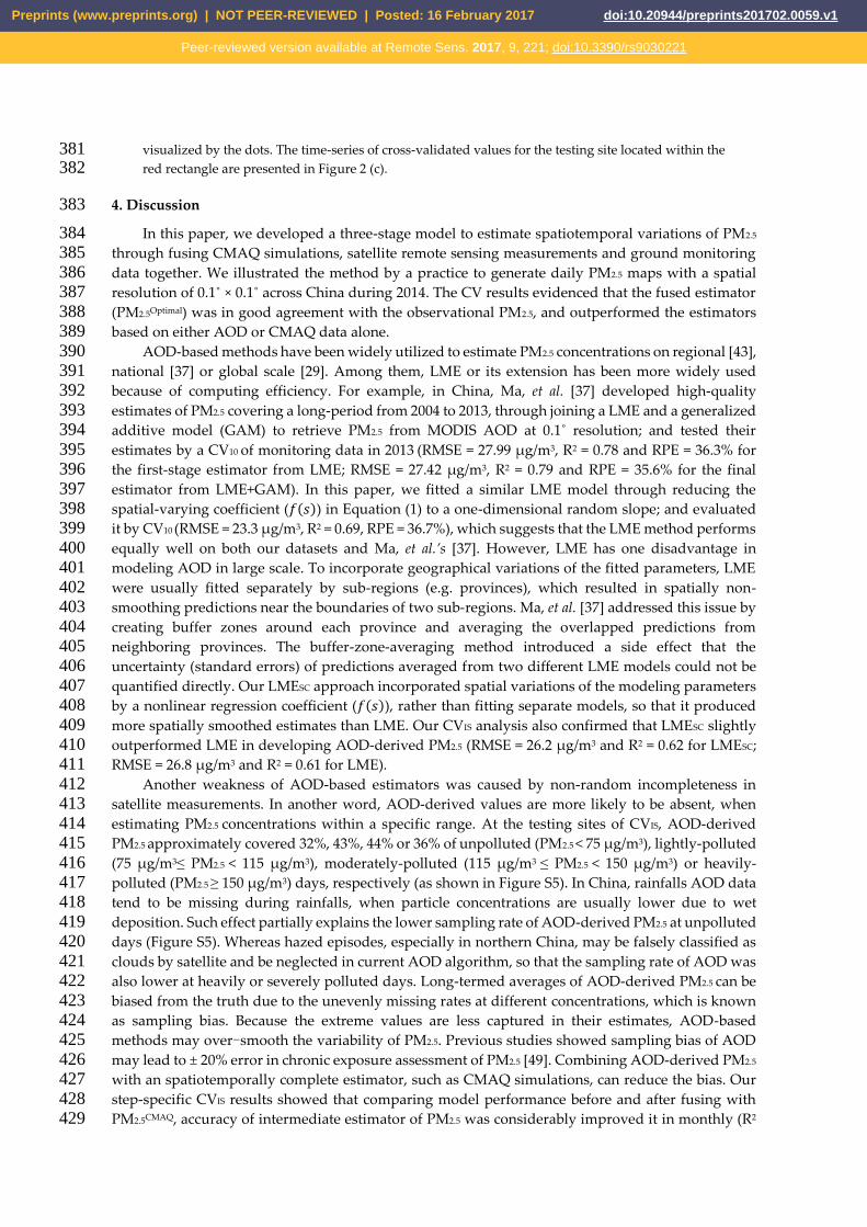
We also explored temporal (Figure S6) and spatial (Figure S7) variations of CVIS results. To 319 evaluate the temporal variation of CVIS errors, we calculated the statistics, including R2, RMSE and 320 NRMSE by dates. The daily CVIS results reflected the final estimator’s capacity to capture spatial 321 variations of PM2.5. The CVIS RMSE for PM2.5Optimal is proportional to the observed value and thus was 322 varied seasonally (higher in colder season, but lower in warmer season). However, we found 323 significantly trend neither in daily NRMSEs nor in daily R2s (Figure S6), which indicates that the 324 accuracy of PM2.5Optimal is temporally constant. Analogously, we also calculated CVIS statistics by sites 325 to evaluate the final estimator’s capacity to capture temporal variations of PM2.5. CVIS results by sites 326 displayed significantly spatial patterns, which indicates that PM2.5Optimal is more accurate in eastern 327 China, but less in western China (Figure S7). Partial reason is that the accuracy of PM2.5Optimal tends to 328 increase with the density of training sites (Figure 8), which are more clustered in eastern China, 329 especially the urban areas (e.g. Yangtze River Delta or Pearl River Delta metropolitan region). 330
Preprints (www.preprints.org) | NOT PEER-REVIEWED | Posted: 16 February 2017 doi:10.20944/preprints201702.0059.v1
Peer-reviewed version available at Remote Sens. 2017, 9, 221; doi:10.3390/rs9030221

331
Figure 4. Scatterplots of cross-validated values and their monthly or annual averages for final 332 estimator (PM2.5Optimal) and intermediate estimators of the three-stage model (PM2.5AOD, PM2.5CMAQ and 333 PM2.5ML). 334
Preprints (www.preprints.org) | NOT PEER-REVIEWED | Posted: 16 February 2017 doi:10.20944/preprints201702.0059.v1
Peer-reviewed version available at Remote Sens. 2017, 9, 221; doi:10.3390/rs9030221

3.3 The fitted spatial and seasonal patterns of PM2.5 in China 335
Figure 5 presents the annual maps of PM2.5 fitted by the three-stage model and its intermediate 336 steps. Different methods displayed consistent patterns in spatial variation of PM2.5, particularly across 337 eastern China, where PM2.5 pollutants were dominated by anthropogenic sources. During 2014, the 338 hot-spots of PM2.5 (PM2.5Optimal = 85~120 μg/m3) spanned over North China Plain (the municipalities of 339 Beijing and Tianjin, and the provinces of Hebei, Henan and Shandong). The moderately polluted 340 areas (PM2.5Optimal = 45~85 μg/m3) occupied Sichuan Basin (Sichuan Province and Chongqing 341 Municipality), Loess Plateau (Shanxi Province and middle of Shaanxi Province), Yangtze Plain 342 (Shanghai Municipality, the provinces of Anhui, Jiangsu, Hunan and Hubei) and Northeast China 343 Plain (the provinces of Heilongjiang, Liaoning and Jilin). The major divergence among these maps 344 exists in the deserted areas of northwestern China. CMAQ-based estimators (i.e. CMAQ-simulated 345 PM2.5 and calibrated-CMAQ PM2.5) failed to capture PM2.5 from natural sources and underestimated 346 the concentrations across the Taklamakan desert. In the fused estimators (i.e. PM2.5ML and PM2.5Optimal), 347 the problem was fixed by introducing AOD data. Figure 6 presents seasonal maps of PM2.5 fitted by 348 PM2.5Optimal, which confirms that PM2.5 concentrations are higher during winter (DJF) and autumn 349 (SON), but lower in summer (JJA) and spring (MAM). The sever pollution of PM2.5 in colder seasons 350 might be attributed by fossil fuel combustions, especially across northern China. Seasonal maps for 351 the other estimators are presented in supplemental Figure S4. 352
353
354
Figure 5. Annual maps (0.1˚ × 0.1˚) of PM2.5 during 2014 over China, produced by CMAQ, 355 intermediate and final estimators of the three-stage model. 356
Preprints (www.preprints.org) | NOT PEER-REVIEWED | Posted: 16 February 2017 doi:10.20944/preprints201702.0059.v1
Peer-reviewed version available at Remote Sens. 2017, 9, 221; doi:10.3390/rs9030221

357
358
Figure 6. Seasonal maps (0.1˚ × 0.1˚) of PM2.5 during 2014 over China, produced by the three-stage 359 model (PM2.5Optimal). 360
3.4 Exposure assessments based on the fused estimates 361
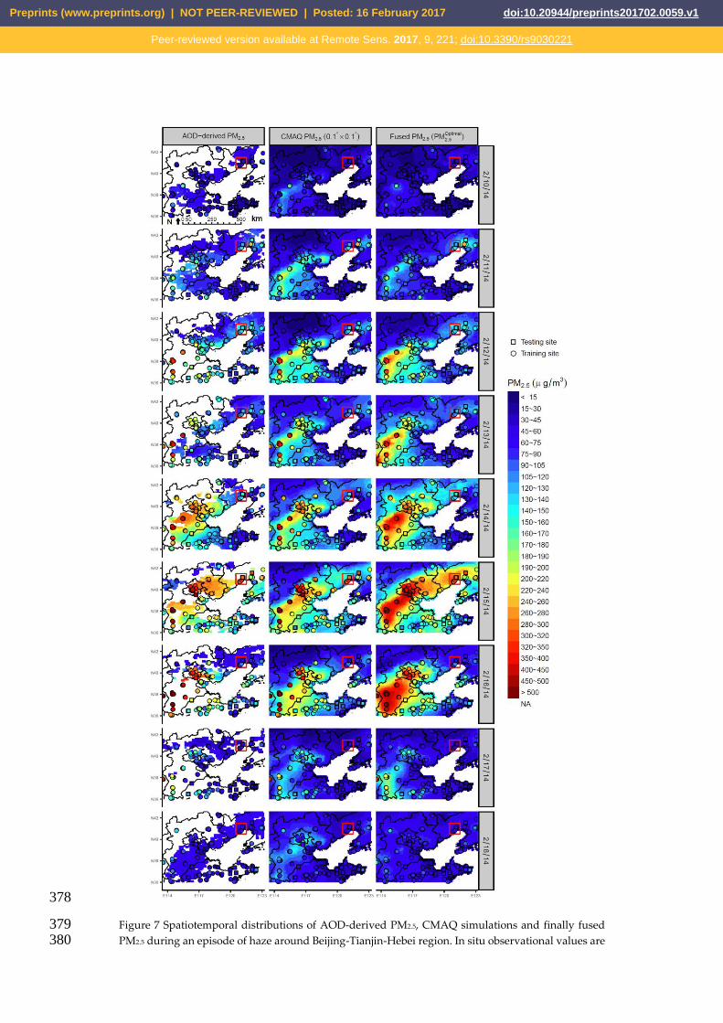
The fused estimator of PM2.5 (PM2.5Optimal) will support exposure assessments in future health-362 related studies. AOD or CMAQ based estimator of PM2.5 has been utilized to study long-term rather 363 than short-term exposure to ambient pollution [18,49], because of data availability or data accuracy 364 on daily scale. For example, we visualized spatiotemporal distributions of CMAQ simulations and 365 AOD-derived PM2.5 with the corresponding monitoring data during an episode of haze around 366 Beijing-Tianjin-Hebei region in Figure 7. According to the maps, AOD-based method overlooked 367 some hotspots due to incompleteness and could not capture the whole polluting procedure; whereas 368 CMAQ simulations underestimated the severity of haze due to systematic errors. Unlike them, the 369 fused estimates accurately characterized the growth, expansion and elimination of the haze. 370 Therefore, PM2.5Optimal can serves as exposure estimates to study either acute or chronic effects of PM2.5. 371 For example, combining PM2.5Optimal with county-level data of China’s sixth census, we assessed both 372 annual and daily exposures to PM2.5 across China in 2014. Accordingly, population-weighted 373 concentration of annual exposure to ambient PM2.5 was 55.7 μg/m3 and 82% of total population 374 inhabited in the places exceeding WHO Air Quality Interim Target-1, 35 μg/m3; whereas population-375 weighted count of polluted or heavily-polluted days (defined as daily mean of PM2.5 > 75 μg/m3 or 376 150 μg/m3 by CNAAQS) was 81 or 14 days, respectively. 377
Preprints (www.preprints.org) | NOT PEER-REVIEWED | Posted: 16 February 2017 doi:10.20944/preprints201702.0059.v1
Peer-reviewed version available at Remote Sens. 2017, 9, 221; doi:10.3390/rs9030221
378
Figure 7 Spatiotemporal distributions of AOD-derived PM2.5, CMAQ simulations and finally fused 379 PM2.5 during an episode of haze around Beijing-Tianjin-Hebei region. In situ observational values are 380
Preprints (www.preprints.org) | NOT PEER-REVIEWED | Posted: 16 February 2017 doi:10.20944/preprints201702.0059.v1
Peer-reviewed version available at Remote Sens. 2017, 9, 221; doi:10.3390/rs9030221
visualized by the dots. The time-series of cross-validated values for the testing site located within the 381 red rectangle are presented in Figure 2 (c). 382
4. Discussion383
In this paper, we developed a three-stage model to estimate spatiotemporal variations of PM2.5 384 through fusing CMAQ simulations, satellite remote sensing measurements and ground monitoring 385 data together. We illustrated the method by a practice to generate daily PM2.5 maps with a spatial 386 resolution of 0.1˚ × 0.1˚ across China during 2014. The CV results evidenced that the fused estimator 387 (PM2.5Optimal) was in good agreement with the observational PM2.5, and outperformed the estimators 388 based on either AOD or CMAQ data alone. 389
AOD-based methods have been widely utilized to estimate PM2.5 concentrations on regional [43], 390 national [37] or global scale [29]. Among them, LME or its extension has been more widely used 391 because of computing efficiency. For example, in China, Ma, et al. [37] developed high-quality 392 estimates of PM2.5 covering a long-period from 2004 to 2013, through joining a LME and a generalized 393 additive model (GAM) to retrieve PM2.5 from MODIS AOD at 0.1˚ resolution; and tested their 394 estimates by a CV10 of monitoring data in 2013 (RMSE = 27.99 μg/m3, R2 = 0.78 and RPE = 36.3% for 395 the first-stage estimator from LME; RMSE = 27.42 μg/m3, R2 = 0.79 and RPE = 35.6% for the final 396 estimator from LME+GAM). In this paper, we fitted a similar LME model through reducing the 397 spatial-varying coefficient (𝑓(𝑠)) in Equation (1) to a one-dimensional random slope; and evaluated 398 it by CV10 (RMSE = 23.3 μg/m3, R2 = 0.69, RPE = 36.7%), which suggests that the LME method performs 399 equally well on both our datasets and Ma, et al.’s [37]. However, LME has one disadvantage in 400 modeling AOD in large scale. To incorporate geographical variations of the fitted parameters, LME 401 were usually fitted separately by sub-regions (e.g. provinces), which resulted in spatially non-402 smoothing predictions near the boundaries of two sub-regions. Ma, et al. [37] addressed this issue by 403 creating buffer zones around each province and averaging the overlapped predictions from 404 neighboring provinces. The buffer-zone-averaging method introduced a side effect that the 405 uncertainty (standard errors) of predictions averaged from two different LME models could not be 406 quantified directly. Our LMESC approach incorporated spatial variations of the modeling parameters 407 by a nonlinear regression coefficient (𝑓(𝑠)), rather than fitting separate models, so that it produced 408 more spatially smoothed estimates than LME. Our CVIS analysis also confirmed that LMESC slightly 409 outperformed LME in developing AOD-derived PM2.5 (RMSE = 26.2 μg/m3 and R2 = 0.62 for LMESC; 410 RMSE = 26.8 μg/m3 and R2 = 0.61 for LME). 411
Another weakness of AOD-based estimators was caused by non-random incompleteness in 412 satellite measurements. In another word, AOD-derived values are more likely to be absent, when 413 estimating PM2.5 concentrations within a specific range. At the testing sites of CVIS, AOD-derived 414 PM2.5 approximately covered 32%, 43%, 44% or 36% of unpolluted (PM2.5 < 75 μg/m3), lightly-polluted 415 (75 μg/m3≤ PM2.5 < 115 μg/m3), moderately-polluted (115 μg/m3 ≤ PM2.5 < 150 μg/m3) or heavily-416 polluted (PM2.5 ≥ 150 μg/m3) days, respectively (as shown in Figure S5). In China, rainfalls AOD data 417 tend to be missing during rainfalls, when particle concentrations are usually lower due to wet 418 deposition. Such effect partially explains the lower sampling rate of AOD-derived PM2.5 at unpolluted 419 days (Figure S5). Whereas hazed episodes, especially in northern China, may be falsely classified as 420 clouds by satellite and be neglected in current AOD algorithm, so that the sampling rate of AOD was 421 also lower at heavily or severely polluted days. Long-termed averages of AOD-derived PM2.5 can be 422 biased from the truth due to the unevenly missing rates at different concentrations, which is known 423 as sampling bias. Because the extreme values are less captured in their estimates, AOD-based 424 methods may over-smooth the variability of PM2.5. Previous studies showed sampling bias of AOD 425 may lead to ± 20% error in chronic exposure assessment of PM2.5 [49]. Combining AOD-derived PM2.5 426 with an spatiotemporally complete estimator, such as CMAQ simulations, can reduce the bias. Our 427 step-specific CVIS results showed that comparing model performance before and after fusing with 428 PM2.5CMAQ, accuracy of intermediate estimator of PM2.5 was considerably improved it in monthly (R2 429
Preprints (www.preprints.org) | NOT PEER-REVIEWED | Posted: 16 February 2017 doi:10.20944/preprints201702.0059.v1
Peer-reviewed version available at Remote Sens. 2017, 9, 221; doi:10.3390/rs9030221

= 0.67 for PM2.5AOD vs. R2 = 0.77 for PM2.5ML) or yearly scale (R2 = 0.73 for PM2.5AOD vs. R2 = 0.81 for 430 PM2.5ML), which may be explained by the reduction of sampling bias. 431
Air quality modeling results have been utilized in risk assessment of ambient pollutants [32] but 432 rarely in epidemiological studies because of their low accuracy and potential bias. Data assimilation 433 methods have been applied to improve predictability of air quality models. In China, Tang, et al. [50] 434 first developed an EnKF to combine numerical outputs from the Nested Air Quality Prediction 435 Modeling System (NAQPMS) [51] and in situ observations of Ozone; then Liu, et al. [18] applied a 436 similar method to estimate daily PM2.5 across China during 2013 and reported a RMSE of 30.2 μg/m3 437 by a five-fold CV, which is as accurate as our intermediate estimator, PM2.5CMAQ (CVIS RSME = 30.1 438 μg/m3). In this study, we improved raw CMAQ estimates (CVIS RSME = 33.4 μg/m3, shown in Figure 439 S3) is three aspects: (1) downscaling spatial resolution of CMAQ simulations to 0.1˚ (CVIS RSME = 440 33.0 μg/m3, shown in Figure S2), (2) calibrating them with in situ observations (CVIS CVIS RSME = 30.1 441 μg/m3 for PM2.5CMAQ, shown in Figure 4 (c)) and (3) fusing them with AOD-derived PM2.5 (CVIS RSME 442 = 28.2 μg/m3 for PM2.5ML, shown in Figure 4(d)). Although the data fusion step increased little on CVIS 443 RMSE, but significantly decreased the bias of CMAQ-based estimator (Bias = 14.8 μg/m3 for PM2.5CMAQ 444 vs. Bias = 7.7 μg/m3 for the PM2.5ML, fused by both PM2.5CMAQ and PM2.5AOD), which reflected that AOD 445 played a key role to control systemic error in data fusion. 446
In the final step of the three-stage model, we incorporated the spatiotemporal variations 447 unexplained by PM2.5ML through modeling the residuals by S/T-Kriging, which is analogous to the 448 GAM stage in Ma, et al. [37]. Kriging has been proved to be mathematically equivalent to thin-plate 449 regression splines, a specific type of GAM [40]. According to CVIS, S/T-Kriging further decreased 450 modeling error by 18% (RMSE = 28.2 μg/m3 for PM2.5ML vs. RMSE = 23.0 μg/m3 for PM2.5Optimal), which 451 indicated that the spatiotemporal autocorrelations should not be ignored in PM2.5 modeling. 452 Additionally, we also found that CVIS errors of PM2.5Optimal tended to be lower at the testing sites, 453 which were surrounded by more training sites (Figure 8). Similar findings have been reported in 454 previous studies, which introduced spatial or spatiotemporal autocorrelations into PM2.5 modeling 455 [52]. 456
Preprints (www.preprints.org) | NOT PEER-REVIEWED | Posted: 16 February 2017 doi:10.20944/preprints201702.0059.v1
Peer-reviewed version available at Remote Sens. 2017, 9, 221; doi:10.3390/rs9030221
457
Figure 8 Different performances of CVIS for the final estimator (PM2.5Optimal) by density of training sites, 458 estimated by a 2-dimensional Kernel with a bandwidth of 50 kilometer. The blue curves and grey 459 ribbons present the LOESS smoothing trends with corresponding confidence intervals. 460
Spatiotemporally autocorrelation-ship benefits prediction of PM2.5, especially at the unmeasured 461 locations but makes troubles for model evaluation. In CVs of auto-correlated variables, randomly 462 selected testing data (e.g. CV10) may not be independent of the training data, so that the predicting 463 accuracy can be overestimated [48]. Through choosing the isolated monitoring sites in CVIS approach, 464 we attempted to use the testing records, which were less correlated with training data. We compared 465 performance of CVIS to that of CV10 in evaluating the AOD-derived PM2.5 from the LME model, as 466 shown in Figure S1. In comparison, we used a subset of CV10 to make sure that the two CVs were 467 conducted on the same testing records. We found that CV10 error of the LME was consistent with the 468 previous studies [37], but considerably lower than CVIS error (CV10 RMSE = 23.3 μg/m3 vs. CVIS RMSE 469 = 26.8 μg/m3). The results suggested that CV10 might overestimate the predicting accuracy. Lv, et al. 470 [48] addressed this issue through leaving out records from all monitors within a city simultaneously 471 in CV, which is analogous to our approach, considering that monitors are usually clustered within 472 cities but separated between different cities. Even though the models were evaluated by CVIS in this 473 paper, the influence of spatiotemporal autocorrelations on CVs cannot be avoided completely. In 474 another word, the true predicting error of the three-stage model may be still underestimated in this 475 paper. 476
The uncertainty of our study sources from three aspects. First, during our study period, the 477 routine monitoring networks for ambient particles were too sparsely distributed to characterize some 478 polluted sub-urban areas, such as undeveloped cities in the provinces of Henan and Shannxi. Second, 479 satellite-derived AOD measurements played a key role to control bias in our approach but were only 480 available at approximately one third of the predicting points. Increasing the spatiotemporal coverage 481 of AOD (e.g., combing AOD from multiple satellites) will be considered in our future studies to 482 reduce modeling uncertainty. Finally, CMAQ-WRF simulating procedures and inputted emission 483 inventories may also contribute to the uncertainty of the three-stage model. 484
Preprints (www.preprints.org) | NOT PEER-REVIEWED | Posted: 16 February 2017 doi:10.20944/preprints201702.0059.v1
Peer-reviewed version available at Remote Sens. 2017, 9, 221; doi:10.3390/rs9030221

5. Conclusions485
We developed a three-stage statistical model to estimate PM2.5 concentrations through fusing in 486 situ observations, satellite-derived AOD measurements and CMAQ simulations. We applied the 487 method to produce daily maps of PM2.5 over China at a spatial resolution of 0.1˚. The final estimator 488 of the three-stage model is shown to highly correlated with daily monitoring data (CVIS R2=0.72) and 489 to outperform CMAQ-simulated PM2.5 (CVIS R2=0.51) or AOD-derived PM2.5 (CVIS R2=0.62). Our 490 estimates will support future health-related studies on either acute or chronic exposure to ambient 491 PM2.5. 492
Supplementary Materials: The following are available online at www.mdpi.com/link, Figure S1: Scatterplots to 493 compare CV10 and CVIS using AOD-derived PM2.5 from a LME model, Figure S2: Scatterplots of cross-validated 494 values and their monthly or annual averages for downscaled CMAQ PM2.5 (0.1˚ × 0.1˚), Figure S3: Scatterplots of 495 cross-validated values and their monthly or annual averages for raw CMAQ PM2.5 (36 km × 36 km), Figure S4: 496 Seasonal maps of PM2.5 in 2014 over China, produced by CMAQ, intermediate and final estimators of the three-497 stage model, Figure S5 Comparisons of coverage rate (CR) of AOD-derived PM2.5 by groups of observational 498 PM2.5 at the CVIS testing sites, Figure S6 Temporal variations of CV results for the final estimator (PM2.5Optimal), 499 Figure S7 Spatial distributions of CV results for the final estimator (PM2.5Optimal), Figure S8 Distributions of 500 coefficients for AOD by months (upper panel) and their spatial patterns by seasons (lower panel) in Equation 501 (1), Figure S9 Distributions of coefficients for CMAQ-simulated PM2.5 by months (upper panel) and their spatial 502 patterns by seasons (lower panel) in Equation (2). 503
Acknowledgments: This work was funded by the National Natural Science Foundation of China (41625020, 504 41571130032, 41222036) and the Public Welfare Program of China's Ministry of Environmental Protection 505 (201509004 and 201309072) for Drs. Zhang, Q. and He, K.. 506
Author Contributions: Dr. Xue, T. designed the statistical models and wrote the paper; Mr. Zheng, Y. simulated 507 CMAQ results and analyzed the satellite data; Dr. Geng, G. analyzed monitoring and satellite data; Dr. Zheng, 508 B. provided emission inventories; Dr. Jiang, X. reviewed literatures; Drs. Zhang, Q. and He, K. designed the 509 whole study. 510
Conflicts of Interest: The authors declare no conflict of interest. 511
References 512
1. Dominici, F.; Peng, R.D.; Bell, M.L.; Pham, L.; Mcdermott, A.; Zeger, S.L.; Samet,513
J.M. Fine particulate air pollution and hospital admission for cardiovascular and514
respiratory diseases. JAMA 2006, 295, 1127-1134.515
2. Peng, R.D.; Bell, M.L.; Geyh, A.S.; Mcdermott, A.; Zeger, S.L.; Samet, J.M.;516
Dominici, F. Emergency admissions for cardiovascular and respiratory diseases and517
the chemical composition of fine particle air pollution. Environmental Health518
Perspectives 2009, 117, 957-963.519
3. Ritz, B.; Yu, F.; Fruin, S.; Chapa, G.; Shaw, G.M.; Harris, J.A. Ambient air pollution520
and risk of birth defects in southern california. American Journal of Epidemiology521
2002, 155, 17-25.522
4. Salam, M.T.; Millstein, J.; Li, Y.; Lurmann, F.; Margolis, H.G.; Gilliland, F.D. Birth523
outcomes and prenatal exposure to ozone, carbon monoxide, and particulate matter:524
Results from the children’s health study. Environmental Health Perspectives 2005,525
113, 1638-1644.526
5. Sapkota, A.; Chelikowsky, A.P.; Nachman, K.E.; Cohen, A.; Ritz, B. Exposure to527
particulate matter and adverse birth outcomes: A comprehensive review and meta-528
analysis. Air Quality, Atmosphere & Health 2010, 5, 369-381.529
Preprints (www.preprints.org) | NOT PEER-REVIEWED | Posted: 16 February 2017 doi:10.20944/preprints201702.0059.v1
Peer-reviewed version available at Remote Sens. 2017, 9, 221; doi:10.3390/rs9030221

6. Wei, Y.; Han, I.; Shao, M.; Hu, M.; Zhang, J.; Tang, X. PM2.5 constituents and530
oxidative DNA damage in humans. Environmental Science & Technology 2009, 43,531
4757-4762.532
7. Ren, C.; Park, S.K.; Vokonas, P.S.; Sparrow, D.; Wilker, E.H.; Baccarelli, A.; Suh,533
H.H.; Tucker, K.L.; Wright, R.O.; Schwartz, J. Air pollution and homocysteine: More534
evidence that oxidative stress-related genes modify effects of particulate air pollution.535
Epidemiology 2010, 21, 198-206.536
8. Laden, F.; Schwartz, J.; Speizer, F.E.; Dockery, D.W. Reduction in fine particulate537
air pollution and mortality: Extended follow-up of the harvard six cities study.538
American Journal of Respiratory and Critical Care Medicine 2006, 173, 667-672.539
9. Pope, C.A.; Burnett, R.T.; Turner, M.C.; Cohen, A.; Krewski, D.; Jerrett, M.; Gapstur,540
S.M.; Thun, M.J. Lung cancer and cardiovascular disease mortality associated with541
ambient air pollution and cigarette smoke: Shape of the exposure–response542
relationships. Environmental Health Perspectives 2011, 119, 1616-1621.543
10. Zhang, J.; Mauzerall, D.L.; Zhu, T.; Liang, S.; Ezzati, M.; Remais, J.V.544
Environmental health in china: Progress towards clean air and safe water. The Lancet545
2010, 375, 1110-1119.546
11. Zhang, Q.; He, K.; Huo, H. Policy: Cleaning china's air. Nature 2012, 484, 161-162.547
12. Wang, Y.; Sun, M.; Yang, X.; Yuan, X. Public awareness and willingness to pay for548
tackling smog pollution in china: A case study. Journal of Cleaner Production 2016,549
112, 1627-1634.550
13. Li, G.X.; Zhou, M.G.; Zhang, Y.J.; Cai, Y.; Pan, X.C. Seasonal effects of PM10551
concentrations on mortality in tianjin, china: A time-series analysis. Journal of Public552
Health 2012, 21, 135-144.553
14. Chen, R.; Zhang, Y.; Yang, C.; Zhao, Z.; Xu, X.; Kan, H. Acute effect of ambient air554
pollution on stroke mortality in the china air pollution and health effects study. Stroke555
2013, 44, 954-960.556
15. Guo, Y.; Li, S.; Tian, Z.; Pan, X.; Zhang, J.; Williams, G.M. The burden of air557
pollution on years of life lost in beijing, china, 2004-08: Retrospective regression558
analysis of daily deaths. BMJ 2013, 347, 1-10.559
16. Yang, Y.; Li, R.; Li, W.; Wang, M.; Cao, Y.; Wu, Z.; Xu, Q. The association between560
ambient air pollution and daily mortality in beijing after the 2008 olympics: A time561
series study. PLOS ONE 2013, 8.562
17. Wu, S.; Deng, F.; Huang, J.; Wang, H.; Shima, M.; Wang, X.; Qin, Y.; Zheng, C.;563
Wei, H.; Yu, H. Blood pressure changes and chemical constituents of particulate air564
pollution: Results from the healthy volunteer natural relocation (hvnr) study.565
Environmental Health Perspectives 2013, 121, 66-72.566
18. Liu, J.; Han, Y.; Tang, X.; Zhu, J.; Zhu, T. Estimating adult mortality attributable to567
PM2.5 exposure in china with assimilated PM2.5 concentrations based on a ground568
monitoring network. Science of The Total Environment 2016, 568, 1253-1262.569
Preprints (www.preprints.org) | NOT PEER-REVIEWED | Posted: 16 February 2017 doi:10.20944/preprints201702.0059.v1
Peer-reviewed version available at Remote Sens. 2017, 9, 221; doi:10.3390/rs9030221

19. Jerrett, M.; Burnett, R.T.; Ma, R.; Pope, C.A.; Krewski, D.; Newbold, K.B.; Thurston,570
G.D.; Shi, Y.; Finkelstein, N.; Calle, E.E. Spatial analysis of air pollution and571
mortality in los angeles. Epidemiology 2005, 16, 727-736.572
20. Mercer, L.D.; Szpiro, A.A.; Sheppard, L.; Lindstrom, J.; Adar, S.D.; Allen, R.; Avol,573
E.L.; Oron, A.P.; Larson, T.V.; Liu, L.J.S. Comparing universal kriging and land-use574
regression for predicting concentrations of gaseous oxides of nitrogen (nox) for the575
multi-ethnic study of atherosclerosis and air pollution (mesa air). Atmospheric576
Environment 2011, 45, 4412-4420.577
21. Henderson, S.B.; Beckerman, B.; Jerrett, M.; Brauer, M. Application of land use578
regression to estimate long-term concentrations of traffic-related nitrogen oxides and579
fine particulate matter. Environmental Science & Technology 2007, 41, 2422-2428.580
22. Eeftens, M.; Beelen, R.; K, D.H.; Bellander, T.; Cesaroni, G.; Cirach, M.; Declercq,581
C.; Dėdelė, A.; Dons, E.; A, D.N. Development of land use regression models for582
PM2.5, PM2.5 absorbance, PM10 and PMcoarse in 20 european study areas; results of the583
escape project. Environmental Science & Technology 2012, 46, 11195-11205.584
23. Martin, R.V. Satellite remote sensing of surface air quality. Atmospheric Environment585
2008, 42, 7823-7843.586
24. Paciorek, C.J.; Liu, Y.; Morenomacias, H.; Kondragunta, S. Spatiotemporal587
associations between goes aerosol optical depth retrievals and ground-level PM2.5.588
Environmental Science & Technology 2008, 42, 5800-5806.589
25. Kloog, I.; Nordio, F.; Coull, B.A.; Schwartz, J. Incorporating local land use regression590
and satellite aerosol optical depth in a hybrid model of spatiotemporal PM2.5591
exposures in the mid-atlantic states. Environmental Science & Technology 2012, 46,592
11913-11921.593
26. Ma, Z.; Hu, X.; Huang, L.; Bi, J.; Liu, Y. Estimating ground-level PM2.5 in china594
using satellite remote sensing. Environmental Science & Technology 2014, 48, 7436-595
7444. 596
27. Beloconi, A.; Kamarianakis, Y.; Chrysoulakis, N. Estimating urban PM10 and PM2.5597
concentrations, based on synergistic meris/aatsr aerosol observations, land cover and598
morphology data ☆. Remote Sensing of Environment 2016, 172, 148-164.599
28. Van Donkelaar, A.; Martin, R.V.; Park, R.J. Estimating ground‐level PM2.5 using600
aerosol optical depth determined from satellite remote sensing. Journal of601
Geophysical Research 2006, 111.602
29. Van Donkelaar, A.; Martin, R.V.; Brauer, M.; Kahn, R.A.; Levy, R.C.; Verduzco, C.;603
Villeneuve, P.J. Global estimates of ambient fine particulate matter concentrations604
from satellite-based aerosol optical depth: Development and application.605
Environmental Health Perspectives 2010, 118, 847-855.606
30. Byun, D.W.; Schere, K.L. Review of the governing equations, computational607
algorithms, and other components of the models-3 community multiscale air quality608
(CMAQ) modeling system. Applied Mechanics Reviews 2006, 59, 51-77.609
Preprints (www.preprints.org) | NOT PEER-REVIEWED | Posted: 16 February 2017 doi:10.20944/preprints201702.0059.v1
Peer-reviewed version available at Remote Sens. 2017, 9, 221; doi:10.3390/rs9030221

31. Nawahda, A.; Yamashita, K.; Ohara, T.; Kurokawa, J.; Yamaji, K. Evaluation of610
premature mortality caused by exposure to PM2.5 and ozone in east asia: 2000, 2005,611
2020. Water Air and Soil Pollution 2012, 223, 3445-3459.612
32. Lelieveld, J.; Evans, J.S.; Fnais, M.; Giannadaki, D.; Pozzer, A. The contribution of613
outdoor air pollution sources to premature mortality on a global scale. Nature 2015,614
525, 367-371.615
33. Bravo, M.A.; Fuentes, M.; Zhang, Y.; Burr, M.J.; Bell, M.L. Comparison of exposure616
estimation methods for air pollutants: Ambient monitoring data and regional air617
quality simulation. Environmental Research 2012, 116, 1-10.618
34. Beckerman, B.S.; Jerrett, M.; Serre, M.L.; Martin, R.V.; Lee, S.; Van Donkelaar, A.;619
Ross, Z.; Su, J.; Burnett, R.T. A hybrid approach to estimating national scale620
spatiotemporal variability of PM2.5 in the contiguous united states. Environmental621
Science & Technology 2013, 47, 7233-7241.622
35. Mcmillan, N.J.; Holland, D.M.; Morara, M.; Feng, J. Combining numerical model623
output and particulate data using bayesian space–time modeling. Environmetrics624
2010, 21, 48-65.625
36. Friberg, M.; Zhai, X.; Holmes, H.A.; Chang, H.H.; Strickland, M.J.; Sarnat, S.E.;626
Tolbert, P.E.; Russell, A.G.; Mulholland, J.A. Method for fusing observational data627
and chemical transport model simulations to estimate spatiotemporally resolved628
ambient air pollution. Environmental Science & Technology 2016, 50, 3695-3705.629
37. Ma, Z.; Hu, X.; Sayer, A.M.; Levy, R.C.; Zhang, Q.; Xue, Y.; Tong, S.; Bi, J.; Huang,630
L.; Liu, Y. Satellite-based spatiotemporal trends in PM2.5 concentrations: China 2004-631
2013. Environmental Health Perspectives 2016, 124, 184-192.632
38. Bey, I.; Jacob, D.J.; Yantosca, R.M.; Logan, J.A.; Field, B.D.; Fiore, A.M.; Li, Q.;633
Liu, H.Y.; Mickley, L.J.; Schultz, M.G. Global modeling of tropospheric chemistry634
with assimilated meteorology: Model description and evaluation. Journal of635
Geophysical Research 2001, 106, 23073-23095.636
39. Zheng, B.; Zhang, Q.; Zhang, Y.; He, K.B.; Wang, K.; Zheng, G.T.; Duan, F.K.; Ma,637
Y.; Kimoto, T. Heterogeneous chemistry: A mechanism missing in current models to638
explain secondary inorganic aerosol formation during the january 2013 haze episode639
in north china. Atmospheric Chemistry and Physics 2015, 15, 2031-2049.640
40. Cressie, N. Statistics for spatial data. Terra Nova 1993, 4, 613-617.641
41. Randriamiarisoa, H.; Chazette, P.; Couvert, P.; Sanak, J.; Megie, G. Relative642
humidity impact on aerosol parameters in a paris suburban area. Atmospheric643
Chemistry and Physics 2006, 6, 1389-1407.644
42. Wang, Z.; Chen, L.; Tao, J.; Zhang, Y.; Su, L. Satellite-based estimation of regional645
particulate matter (PM) in beijing using vertical-and-rh correcting method. Remote646
Sensing of Environment 2010, 114, 50-63.647
43. Zheng, Y.; Zhang, Q.; Liu, Y.; Geng, G.; He, K. Estimating ground-level PM2.5648
concentrations over three megalopolises in china using satellite-derived aerosol649
optical depth measurements. Atmospheric Environment 2016, 124, 232-242.650
Preprints (www.preprints.org) | NOT PEER-REVIEWED | Posted: 16 February 2017 doi:10.20944/preprints201702.0059.v1
Peer-reviewed version available at Remote Sens. 2017, 9, 221; doi:10.3390/rs9030221

44. Cressie, N.; Johannesson, G. Fixed rank kriging for very large spatial data sets.651
Journal of The Royal Statistical Society Series B-statistical Methodology 2008, 70,652
209-226.653
45. Wood, S. Generalized additive models: An introduction with r. CRC press: 2006.654
46. Cressie, N.; Wikle, C.K. Statistics for spatio-temporal data. John Wiley & Sons: 2015.655
47. Bunke, O.; Droge, B. Bootstrap and cross-validation estimates of the prediction error656
for linear regression models. Annals of Statistics 1984, 12, 1400-1424.657
48. Lv, B.; Hu, Y.; Chang, H.H.; Russell, A.G.; Bai, Y. Improving the accuracy of daily658
pm2. 5 distributions derived from the fusion of ground-level measurements with659
aerosol optical depth observations, a case study in north china. Environmental science660
& technology 2016, 50, 4752-4759.661
49. Geng, G.; Zhang, Q.; Martin, R.V.; van Donkelaar, A.; Huo, H.; Che, H.; Lin, J.; He,662
K. Estimating long-term PM2.5 concentrations in china using satellite-based aerosol663
optical depth and a chemical transport model. Remote Sensing of Environment 2015,664
166, 262-270.665
50. Tang, X.; Zhu, J.; Wang, Z.; Gbaguidi, A. Improvement of ozone forecast over beijing666
based on ensemble kalman filter with simultaneous adjustment of initial conditions667
and emissions. Atmospheric Chemistry and Physics 2011, 11, 12901-12916.668
51. Wang, Z.; Maeda, T.; Hayashi, M.; Hsiao, L.-F.; Liu, K.-Y. A nested air quality669
prediction modeling system for urban and regional scales: Application for high-ozone670
episode in taiwan. Water, Air, and Soil Pollution 2001, 130, 391-396.671
52. Lee, S.-J.; Serre, M.L.; van Donkelaar, A.; Martin, R.V.; Burnett, R.T.; Jerrett, M.672
Comparison of geostatistical interpolation and remote sensing techniques for673
estimating long-term exposure to ambient PM2.5 concentrations across the continental674
united states. Environmental health perspectives 2012, 120, 1727.675
© 2017 by the authors; licensee Preprints, Basel, Switzerland. This article is an open access article distributed under the terms and conditions of the Creative Commons by Attribution (CC-BY) license (http://creativecommons.org/licenses/by/4.0/).
Preprints (www.preprints.org) | NOT PEER-REVIEWED | Posted: 16 February 2017 doi:10.20944/preprints201702.0059.v1
Peer-reviewed version available at Remote Sens. 2017, 9, 221; doi:10.3390/rs9030221


![Initiation Fusing[1]](https://static.fdocuments.us/doc/165x107/577ce0e11a28ab9e78b44e50/initiation-fusing1.jpg)