FUSED DEPOSITION MODELING WITH LOCALIZED PRE-DEPOSITION

HEATING USING FORCED AIR

by

Seth Collins Partain

A thesis submitted in partial fulfillment of the requirements for the degree

of

Master of Science

in

Mechanical Engineering

MONTANA STATE UNIVERSITY Bozeman, Montana

January 2007

© Copyright

by

Seth Collins Partain

2007

All Rights Reserved

ii

APPROVAL

of the thesis submitted by

Seth Collins Partain

This thesis has been read by each member of the thesis committee and has been found to be satisfactory regarding content, English usage, format, citations, bibliographic style, and consistency, and is ready for submission to the Division of Graduate Education.

Dr. Douglas Cairns, Committee Chair

Approved for the Department of Mechanical and Industrial Engineering

Dr. Christopher H. M. Jenkins, Department Head

Approved for the Division of Graduate Education

Dr. Carl A. Fox, Vice Provost

iii

STATEMENT OF PERMISSION TO USE

In presenting this thesis in partial fulfillment of the requirements for a master’s

degree at Montana State University, I agree that the Library shall make it available to

borrowers under the rules of the library.

If I have indicated my intention to copyright this thesis by including a copyright

notice page, copying is allowable only for scholarly purposes, consistent with “fair use”

as described by U.S. Copyright Law. Requests for permission for extended quotation

from or reproduction of this thesis in whole or in parts may be granted only by the

copyright holder.

Seth Collins Partain

January 2007

iv

ACKNOWLEDGEMENTS

There are many people without whom this project would not have been

completed. I would especially like to thank Dr. Douglas Cairns and Greg Merchant for

their considerable assistance and guidance on this project. In addition, I would like to

acknowledge Jay Smith, James Schmidt, Jesse Law, Pat Vowell, Dr. Alan George, Robb

Larson, Dr. Ahsan Mian, and Dr. Vic Cundy for their valuable support in various aspects

of this work.

I would like to dedicate this thesis to my wife, Tammy.

v

TABLE OF CONTENTS

1. INTRODUCTION ..........................................................................................................1

Fused Deposition Modeling ............................................................................................3 FDM - Potential for Rapid Manufacturing .....................................................................5 Literature Review............................................................................................................7 Description of Bonding Process....................................................................................10 Goals Of The Thesis .....................................................................................................14

2. PRE-DEPOSITION HEATING SYSTEM...................................................................15

Requirements & Considerations ...................................................................................15 System Alternatives ......................................................................................................16 Heating System .............................................................................................................18 Mounting and Heat Delivery Hardware: Welder to the Deposition Head....................20 Mounting and Heat Delivery Hardware: Deposition Head to Substrate.......................24

3. EXPERIMENTAL DESIGN ........................................................................................31

4. EXPERIMENTAL DESIGN ........................................................................................31

Test Part Design ............................................................................................................31 Analysis of Variance (ANOVA)...................................................................................33 Experimental Design.....................................................................................................37 PDHS Characterization for Temperature and Air Speed ..............................................42 Fabrication & Test Procedure .......................................................................................43

5. RESULTS AND ANALYSIS.......................................................................................46

Dimensional Accuracy..................................................................................................47 Material Properties ........................................................................................................49 Interlayer Part Strength .................................................................................................56 SEM Photography .........................................................................................................60 Additional Testing.........................................................................................................64

6. CONCLUSIONS, RECOMMENDATIONS, AND FUTURE WORK .......................69

Conclusions...................................................................................................................69 Recommendations and Future Work.............................................................................74

REFERENCES CITED......................................................................................................76

vi

TABLE OF CONTENTS - CONTINUED

APPENDICES ...................................................................................................................80

APPENDIX A: EQUIPMENT, MATERIAL INFORMATION...............................81 APPENDIX B: ANOVA CALCULATIONS........................................................... .85 APPENDIX C: EXIT FLOW RATE CALCULATIONS....................................... ..92

vii

LIST OF TABLES

Table Page

1. ANOVA table for one-way classification......................................................... 34

2. ANOVA table for two-factor experiment......................................................... 35

3. Description of the experiment treatment levels.................................................41

4. Temperature statistics for PDHS experiment voltages..................................... 43

5. Exit air flow rates.............................................................................................. 43

6. ANOVA table for one-factor analysis of dimensional accuracy.......................48

7. ANOVA table for two-factor analysis of dimensional accuracy...................... 49

8. ANOVA table for one-factor analysis of flexural strength............................... 54

9. ANOVA table for two-factor analysis of flexural strength...............................55

10. ANOVA table for one-factor analysis of interlayer strength.......................... 57

11. ANOVA table for two-factor analysis of interlayer strength.......................... 59

12. Summary of one-factor analyses.....................................................................59

13. Summary of two-factor analyses....................................................................60

viii

LIST OF FIGURES

Figure Page

1. Procedure for rapid prototyping............................................................................ 2

2. Fused Deposition Modeling.................................................................................. 4

3. Anisotropy of FDM parts...................................................................................... 7

4. PVC welder temperature test setup..................................................................... 19

5. Temperature test results for welder at full power............................................... 19

6. Welder and frame, unmounted and mounted configurations.............................. 23

7. One-nozzle design for air delivery hardware...................................................... 25

8. Aborted part made with one-nozzle design.........................................................26

9. Two-nozzle design for air delivery hardware..................................................... 27

10. Strip of thermal paper used to check position of air flows............................... 29

11. CAD model of the test part............................................................................... 32

12. Results diagram for Duncan multiple-range test...............................................37

13. Test parts created to aid in the selection of PDHS treatment levels................. 38

14. Exit air temperatures at PDHS experiment voltages.........................................42

15. Parts created at different PDHS settings........................................................... 46

16. Dimensional accuracy of FDM parts................................................................ 47

17. Duncan diagram for dimensional accuracy (one-factor experiment)................48

18. Duncan diagram for dimensional accuracy (two-factor experiment)................49

19. Delaminated tensile test specimen in the axial direction.................................. 50

ix

LIST OF FIGURES - CONTINUED

Figure Page

20. Flexure test specimens...................................................................................... 51

21. Flexure test specimen setup in three-point bending.......................................... 52

22. Force-displacement curves for axial and transverse specimens........................52

23. Flexure test results for specimens oriented in the axial direction..................... 53

24. Flexure test results for specimens oriented in the transverse direction.............54

25. Duncan diagram for one-factor analysis of flexural strength............................55

26. Sample of force-displacement curves from the interlayer tensile tests............. 56

27. Maximum stress values for interlayer strength in FDM parts...........................57

28. Duncan diagram for one-factor analysis of interlayer strength.........................58

29. Duncan diagram using different PDHS voltages.............................................. 59

30. SEM image, at x65 magnification, part fabricated at 0V/20.68 kPa/650 C...... 61

31. SEM image, at x65 magnification, part fabricated at 0V/0 kPa/700 C..............61

32. SEM image, at x65 magnification, part fabricated at 90V/10.34 kPa/650 C.....62

33. SEM image, at x1000 magnification, part fabricated at 0V/20.68 kPa/650C....62

34. SEM image, at x1000 magnification, part fabricated at 0V/0 kPa/700C...........63

35. SEM image, at x1000 magnification, part fabricated at 90V/10.34 kPa/650C...63

36. Dimensional accuracy for all samples...............................................................65

37. Flexure strength in the axial direction for all samples...................................... 66

38. Interlayer strength of all samples...................................................................... 67

x

LIST OF FIGURES - CONTINUED

Figure Page

39. Testing and analysis hierarchy.......................................................................... 73

xi

ABSTRACT

Rapid prototyping (RP) systems have been used for several years to produce design prototypes without expensive tooling costs. As these systems have matured, there has been increasing interest in using them to produce actual end-use parts. Fused deposition modeling (FDM) is an RP technology that has been identified by many as having strong potential for this transition from rapid prototyping to rapid manufacturing, due primarily to its capability of using a wide array of high performance materials. FDM creates parts layer-by-layer, extruding semi-molten material “roads” through a computer-controlled nozzle onto the substrate, which is mounted on an indexing platform. This manufacturing process creates anisotropic parts, with strength properties greater along material roads than across roads or between layers.

This study proposes to improve FDM part strength in the transverse directions by increasing the amount of material bonding taking place between road and layers through the addition of a system which re-heats the substrate material immediately preceding deposition. To test this concept, a simple pre-deposition heating system (PDHS) was designed, implemented, and tested, measuring part properties in the axial and transverse directions and part dimensional accuracy. The test results were analyzed using statistical techniques, and found that parts made with the PDHS were not significantly stronger in the transverse direction than parts made without the PDHS. The development of the system and test results illustrate the challenges of implementing a PDHS system and lead to a set of recommendations for the next design iteration of PDHS.

1

INTRODUCTION

Rapid prototyping (RP) is a system of technologies aimed at producing physical

prototypes directly from a digital design, bypassing the lengthy (and costly) traditional

prototyping process—which often involves the design and fabrication of molds, jigs, and

fixtures prior to actual prototype production. RP emerged in 1987 [1] and was first

commercialized in 1988 with the introduction of a stereolithography (SLA) system by 3D

Systems [2]. In the years that have followed, numerous systems and technologies have

been introduced. The most prominent category of RP systems are known as solid

freeform fabrication (SFF), of which the most common systems are known as layered

manufacturing (LM) technologies, due to the way parts are created by adding material in

a layer-by-layer fashion.

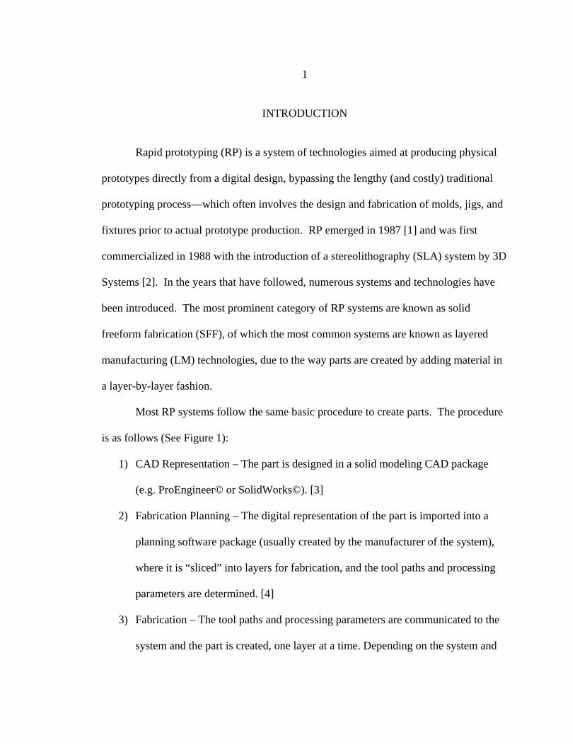
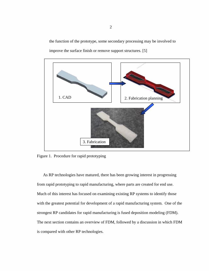
Most RP systems follow the same basic procedure to create parts. The procedure

is as follows (See Figure 1):

1) CAD Representation – The part is designed in a solid modeling CAD package

(e.g. ProEngineer© or SolidWorks©). [3]

2) Fabrication Planning – The digital representation of the part is imported into a

planning software package (usually created by the manufacturer of the system),

where it is “sliced” into layers for fabrication, and the tool paths and processing

parameters are determined. [4]

3) Fabrication – The tool paths and processing parameters are communicated to the

system and the part is created, one layer at a time. Depending on the system and

2

the function of the prototype, some secondary processing may be involved to

improve the surface finish or remove support structures. [5]

Figure 1. Procedure for rapid prototyping

As RP technologies have matured, there has been growing interest in progressing

from rapid prototyping to rapid manufacturing, where parts are created for end use.

Much of this interest has focused on examining existing RP systems to identify those

with the greatest potential for development of a rapid manufacturing system. One of the

strongest RP candidates for rapid manufacturing is fused deposition modeling (FDM).

The next section contains an overview of FDM, followed by a discussion in which FDM

is compared with other RP technologies.

1. CAD 2. Fabrication planning

3. Fabrication

3

Fused Deposition Modeling

Fused deposition modeling is a rapid prototyping technology that extrudes a semi-

molten filament material through a robotically controlled nozzle. Manufactured by

Stratasys Corporation©, FDM follows the basic production procedure outlined above: a

solid CAD model of the part is imported into QuickSlice© (in an .stl format), the

proprietary FDM planning software developed by Stratasys, where it is “sliced” into

layers and a tool-path for each layer is generated. [6]. The part “slices” are determined

by the software according to processing parameters entered by the user and depending on

the FDM hardware being used to fabricate the part (nozzle size, material, etc.). The user-

set parameters, such as row height, deposition speed, and raster angles, allow the user to

tailor the fabrication to suit the needs of the part. For example, there is a “Fast Build”

setting that minimizes the amount of interior material—creating a weaker part—in order

to minimize the fabrication time; this option would be desirable for a user needing a

quick, visual prototype where part strength and durability are not needed [7]. Within the

software, tool-path planning is done in three steps: dividing the CAD model into layers

(this creates a .ssl file), model material tool-path generation, and support material tool-

path generation. The instructions containing the toolpath information are coded in a .sml

file, which is sent to the FDM machine [8].

Once the toolpath information has been sent to the FDM machine, a filament

model material (e.g. ABS plastic) is pulled by rollers into a heated liquefier, where it is

melted and extruded through a nozzle onto a substrate platform. This nozzle, known as

4

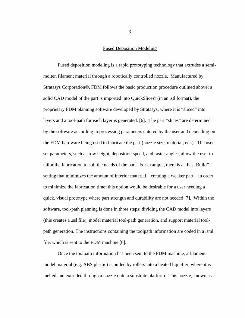
the model material nozzle, is guided in the x-y plane and lays down the material along the

model material tool-path for each layer (the extruded material is known as a “road”).

Figure 2. Fused Deposition Modeling

When one layer is complete (i.e. all of the roads planned for one level have been

deposited), the substrate platform indexes in the z direction, and the nozzle lays down the

next layer. That is, each layer is comprised of a sequence of roads, and the structure is

built up as a sequence of layers. This process is contained within a thermally controlled

environment, which is maintained to a user-set temperature. Figure 2 contains an

illustration of the FDM deposition head, which guides the deposition nozzles. A support

material is deposited through an adjacent nozzle (not shown in the diagram) along the

support material tool-path generated by the software. The purpose of the support material

is to allow for more complex shapes to be produced. Support material is manually

Deposition Head

Material Filament

Drive Wheels

Deposited Material (Roads)

Heater Fan Liquefier

z

y

5

removed as a secondary operation. There is also a water soluble support material

available that would allow the support material to be removed by soaking in a water bath.

FDM - Potential for Rapid Manufacturing

FDM has numerous strengths that make it an attractive candidate for rapid

manufacturing. In order to better understand these strengths, it is useful to briefly

describe two of the most popular alternatives to FDM for rapid prototyping:

stereolithography and 3D printing.

1. Stereolithography (SLA) – Fabricates parts through the use of an ultraviolet

laser, which hardens layers of a light-sensitive liquid resin photopolymer to

form a part. These systems are manufactured by 3D Systems. [9]

2. 3D Printing (3DP) - A powdered material is distributed one thin layer at a time

and selectively hardened and joined together by depositing drops of binder from

an inkjet print head. For each layer, a powder hopper and roller system

distributes a thin layer of powder over the top of the work tray. The inkjet

nozzles than apply binder in parallel in a back-and-forth scan of the entire work

area. This technology was developed at MIT in the late 1980’s and

commercialized by Z Corporation. [10]

The greatest advantage that FDM has over SLA and 3DP is that a wide variety of

materials can be used to create parts. The first commercialized material for FDM was a

grade of acrylonitrile-butadiene-styrene (ABS) plastic, but many other engineering

structural materials are now available, including polycarbonate, polyphenylsulfone,

6

polyester, and a wax material for investment casting [11]. In addition, several studies

have been conducted where FDM or modified FDM technology was used to create parts

using ceramic [12], metal [13], and biomedical materials [14]. In contrast, SLA and 3DP

have greater restrictions on build materials (SLA, for example, builds parts by curing a

light-sensitive polymer with an ultraviolet light—so build materials must possess this

light sensitivity). Since FDM can use high performance engineering materials, FDM

parts are much stronger, more durable, and have greater stability (i.e. parts do not warp or

curl with time or changes in environment) than parts produced using SLA or 3DP. In

addition, FDM is capable of better dimensional accuracy than most other RP technologies

and is cheaper to install and maintain than SLA or 3DP [15, 2].

The strengths of FDM—especially part strength, durability, and material flexibility—

make a strong case for its use in rapid manufacturing compared to other RP systems.

However, there are significant issues that must be resolved before FDM can make the

transition to rapid manufacturing. Current FDM systems produce parts with a rougher

surface finish than other RP technologies, and FDM parts often suffer from both surface

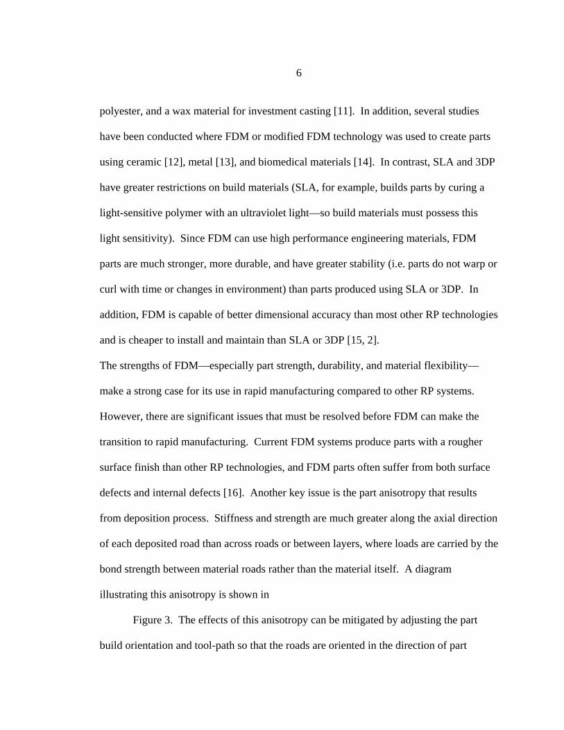
defects and internal defects [16]. Another key issue is the part anisotropy that results

from deposition process. Stiffness and strength are much greater along the axial direction

of each deposited road than across roads or between layers, where loads are carried by the

bond strength between material roads rather than the material itself. A diagram

illustrating this anisotropy is shown in

Figure 3. The effects of this anisotropy can be mitigated by adjusting the part

build orientation and tool-path so that the roads are oriented in the direction of part

7

loading, but any incidental or unforeseen transverse loads could result in the failure of the

part. This anisotropy is a major concern if FDM is used

Figure 3. Anisotropy of FDM parts.

to make functional parts, and any improvements to the interlayer or inter-road bond strength will greatly improve part performance.

Literature Review Given the potential for FDM in the field of rapid manufacturing, there have been

(and continue to be) numerous studies conducted on FDM, exploring ways to use,

optimize, and improve the fused deposition process to create functional parts. A large

portion of this work has focused on improving part quality. Agarwala et al. investigated

the structural quality of fused deposition ceramic and metal parts, and formulated

Strength in road direction: Loads are carried by material.

Strength across roads and layers: Loads are carried by material bonds.

Deposition nozzle

8

deposition strategies to eliminate internal and surface flaws [17]. In a similar vein, Han

et al. developed algorithms to optimize layer evenness and quality through tool-path

planning [18]. A follow-up study by Han et al. used similar tool-path planning algorithms

to speed up part deposition without sacrificing part quality [19]. Langrana et al.

developed a virtual simulation and video microscopy system to monitor the quality of

FDM parts in real time [20]. Anitha et al. studied part quality from the standpoint of

surface finish (rather than the presence of defects) using a statistical analysis of variation

which measured the effects of processing parameters on surface roughness [21].

Another section of work has focused on innovative applications and materials for

FDM. Bose et al. and Darsell et al. both explore the use of FDM in producing scaffold

structures for biomedical applications [22, 23]. Shofner et al. developed a nanofiber-

reinforced ABS feedstock material for FDM, which resulted in significant increases in

part stiffness and strength [24]. Bellini et al. and Wu et al. report on significant work by a

research group based at Rutgers University, exploring the use of fused deposition

technology to produce functional ceramic and metallic parts [12, 25]. Yan et al. use

fused deposition technology with biomaterials to create scaffolding for organ

regeneration [26].

Finally, much of the current literature addresses characterization, modeling, and

optimization of FD part stiffness and strength. Bellini and Güçeri characterized FDM

parts by modeling the parts as an orthotropic material and conducting tensile tests to

determine the appropriate material constants [27]. Rodriguez, Thomas, et al. produced a

series of articles resulting from an extensive research program aimed at developing a

9

design tool for optimizing the mechanical performance of parts produced using fused

deposition. This study included a characterization of the microstructure [28] and

mesostructure [29] of fused deposition ABS (FD-ABS) parts, an investigation of bond

strength in FD-ABS parts [30], the development of a model to predict the stiffness and

strength of FD-ABS parts [31], and the development of an optimization algorithm, which

incorporates the previous work to maximize part performance [32]. Kulkarni and Dutta

examined the effects of deposition strategies on FDM part stiffness and used laminate

theory to model the stiffness of FDM parts produced using a raster tool-path [33]. Yan et

al. conducted a study analyzing bond strength in fused deposition wax parts as a function

of processing parameters and developed a variable, bonding potential, to measure the

bonding interface status [34].

This review of the literature illustrates a gap in the discussion of improving FD

part strength in the transverse direction. The majority of the current literature looking to

improve FDM part performance does so from the standpoint of either tool-path planning

or enhanced materials, rather than hardware or deposition process improvements. Of the

articles reviewed above, only two (Rodriguez et al. [30] and Yan et al. [34]) address

interlayer part strength directly. Both of these studies explore bond strength or bond

toughness as a function of the existing hardware and process parameters, seeking to both

characterize and optimize interlayer and inter-road strength. The findings of these studies

illustrate the processing parameters critical to developing strong material bonds. The

next section contains a discussion of the bonding process that occurs during fused

deposition modeling, which draws upon these works to set up the goal of this research.

10

Description of Bonding Process

The deposition process used by FDM to fabricate parts—bonding polymer roads

and layers to create the part geometry—is essentially an extension of thermoplastic

welding. The bonds created during such a process are formed through molecular bonding

via the interpenetration of molecular chains across a bonding interface. As this

interpenetration increases, the interface gradually disappears and bond strength develops.

This process is a type of mass diffusion and is thermally activated, only occurring at

temperatures above a critical temperature, Tc. There is a slight disagreement in the

literature about this critical temperature: Rodriguez et al. use the glass transition

temperature, Tg [37], while Yan et al. use the Vicat softening temperature as the critical

bonding temperature [38]. In this work, this disagreement regarding which material

paramter is the critical temperature is relatively unimportant—the material under

investigation is an amorphous polymer (ABSi 500), so the values for the glass transition

temperature and the Vicat softening temperature are relatively close together (940 C and

98-1000 C, respectively [37,39]).

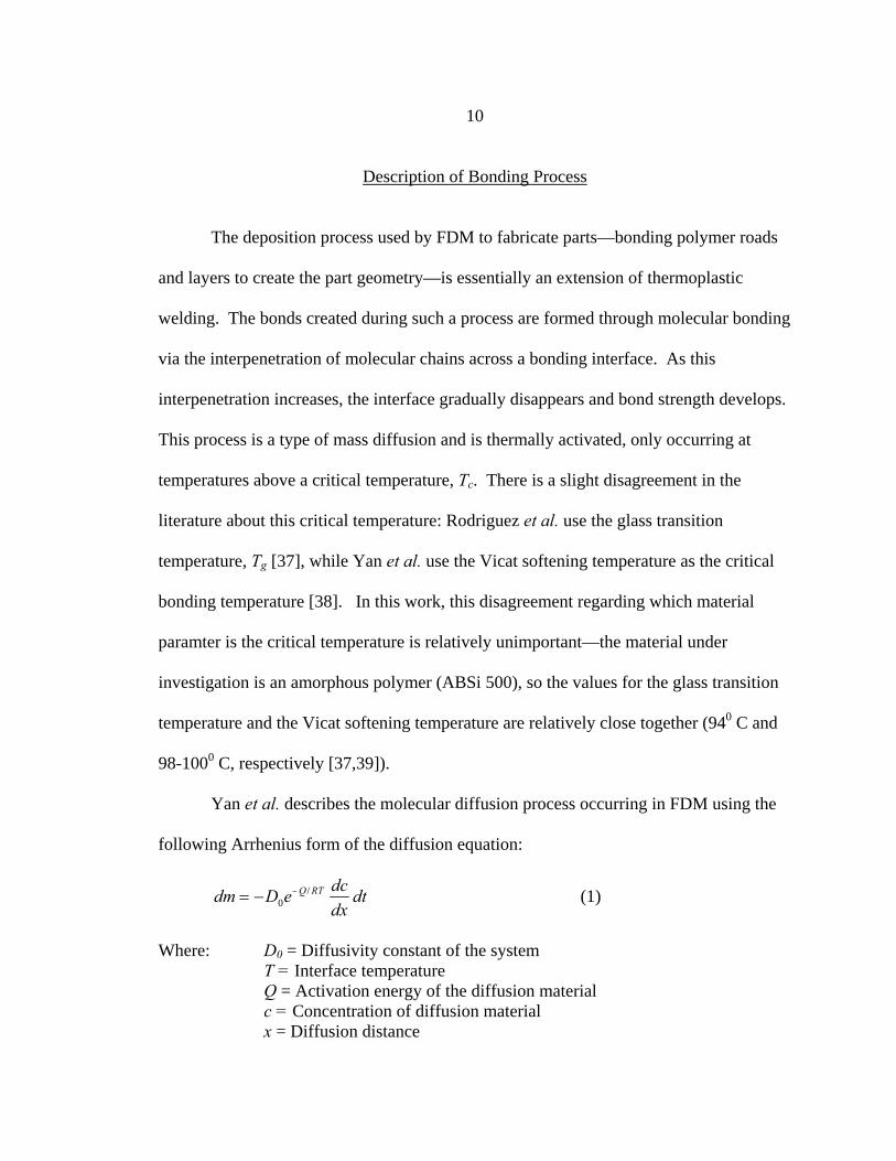
Yan et al. describes the molecular diffusion process occurring in FDM using the

following Arrhenius form of the diffusion equation:

dm D e dcdx

dtQ RT= − −0

/ (1)

Where: D0 = Diffusivity constant of the system T = Interface temperature

Q = Activation energy of the diffusion material c = Concentration of diffusion material x = Diffusion distance

11

R = Gas constant

The concentration gradient dc/dx changes in a complicated fashion, making it difficult in

practice to accurately measure or calculate the interface bonding status with the accurate

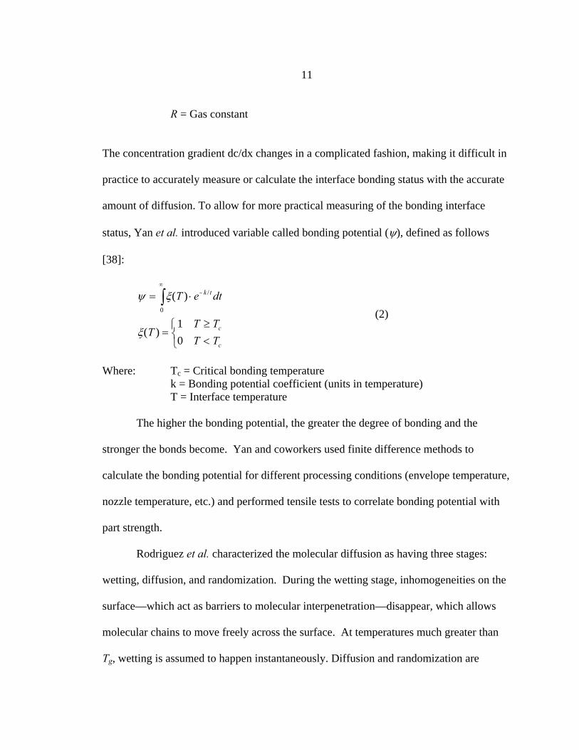
amount of diffusion. To allow for more practical measuring of the bonding interface

status, Yan et al. introduced variable called bonding potential (ψ), defined as follows

[38]:

ψ ξ

ξ

= ⋅

=≥<

⎧⎨⎩

−∞

∫ ( )

( )

/T e dt

TT TT T

k t

c

c

0

10

(2)

Where: Tc = Critical bonding temperature k = Bonding potential coefficient (units in temperature) T = Interface temperature

The higher the bonding potential, the greater the degree of bonding and the

stronger the bonds become. Yan and coworkers used finite difference methods to

calculate the bonding potential for different processing conditions (envelope temperature,

nozzle temperature, etc.) and performed tensile tests to correlate bonding potential with

part strength.

Rodriguez et al. characterized the molecular diffusion as having three stages:

wetting, diffusion, and randomization. During the wetting stage, inhomogeneities on the

surface—which act as barriers to molecular interpenetration—disappear, which allows

molecular chains to move freely across the surface. At temperatures much greater than

Tg, wetting is assumed to happen instantaneously. Diffusion and randomization are

12

described by the reptation model introduced by De Gennes, where polymer molecules

move and back and forth along their backbones in a snake-like Brownian motion [40].

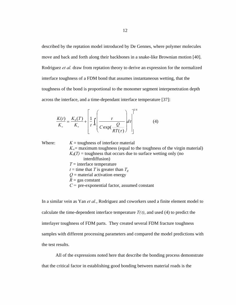
Rodriguez et al. draw from reptation theory to derive an expression for the normalized

interface toughness of a FDM bond that assumes instantaneous wetting, that the

toughness of the bond is proportional to the monomer segment interpenetration depth

across the interface, and a time-dependant interface temperature [37]:

K tK

K TK t C Q

RT

dt( ) ( )

exp(( )

/

∞ ∞

= +

⎛

⎝

⎜⎜⎜⎜

⎞

⎠

⎟⎟⎟⎟

⎡

⎣

⎢⎢⎢⎢

⎤

⎦

⎥⎥⎥⎥

∫00

1 4

1 τ

τ

τ (4)

Where: K = toughness of interface material K∞= maximum toughness (equal to the toughness of the virgin material) K0(T) = toughness that occurs due to surface wetting only (no

interdiffusion) T = interface temperature

t = time that T is greater than Tg

Q = material activation energy R = gas constant C = pre-exponential factor, assumed constant

In a similar vein as Yan et al., Rodriguez and coworkers used a finite element model to

calculate the time-dependent interface temperature T(τ), and used (4) to predict the

interlayer toughness of FDM parts. They created several FDM fracture toughness

samples with different processing parameters and compared the model predictions with

the test results.

All of the expressions noted here that describe the bonding process demonstrate

that the critical factor in establishing good bonding between material roads is the

13

interface temperature—the longer the interface temperature is above the critical

temperature, the greater the strength of the material bond. The results of the two studies

examined here reflect this relationship. Both found that the process parameters most

critical to the interlayer bond strength or toughness were those that affected the interface

temperature: the envelope temperature, Te, and the convection constant, h, within the

envelope. These parameters control the rate of cooling of a newly deposited road or

layer, which becomes the substrate for the next layer or road. The nozzle temperature,

Tn, also plays a role in bond strength as it controls the amount of energy transferred to the

road/base system, but both studies found that Te affected bond strength more than Tn.

Rodriguez et al. determined that the parts created at Te= 1580 F (700 C), the highest

envelope temperature the machine is capable of maintaining, had the best interlayer

performance.

The findings of these studies have large ramifications on the use of FDM for rapid

manufacturing. The dependence of bond strength on maintaining a high environment

temperature and low convection constant, as in the current process, would make it

necessary to keep the deposition environment in an insulated, thermally controlled

envelope. This envelope then becomes a constraint on the size of part that can be

produced. In addition, the interlayer strength will vary due to the size of the part being

fabricated: large parts require more time between layers than small parts, which allows

the substrate more time to cool between layers and will result in weaker interlayer

strength.

14

Goals Of The Thesis

The goal of this research was to develop a system to heat the substrate material

prior to deposition. This heating process is designed to raise the interface temperature

above the critical level where bonding occurs, increasing both the degree of to which

bonding occurs and the strength of these bonds, resulting in greater transverse strength in

FD-ABS parts. Although it is impossible to anticipate all of the ramifications of adding

this additional heat to the process, there are two potential adverse effects that are

immediately identifiable. The first is that excessive heat can cause degradation and

material instability of the feedstock material, leading to a loss of properties. The other is

that maintaining the part at too high of a temperature may prevent the material from

solidifying enough to support additional layers, causing the part to slump and damaging

the dimensional accuracy of the process. With these considerations in mind, the work

was divided into two phases: design and implementation of a Pre-Deposition Heating

System (PDHS) and analysis of the system through statistical methods.

The remainder of this thesis contains a description of the procedure and results of

the two work phases listed above. A description of the pre-deposition heating system,

including the design considerations, system development, and limitations is given in the

next chapter. A discussion follows on the experimental design and testing procedure for

analyzing the effects of the pre-deposition heat system. Finally, the results are discussed

and recommendations are made for additional work in this area.

15

PRE-DEPOSITION HEATING SYSTEM

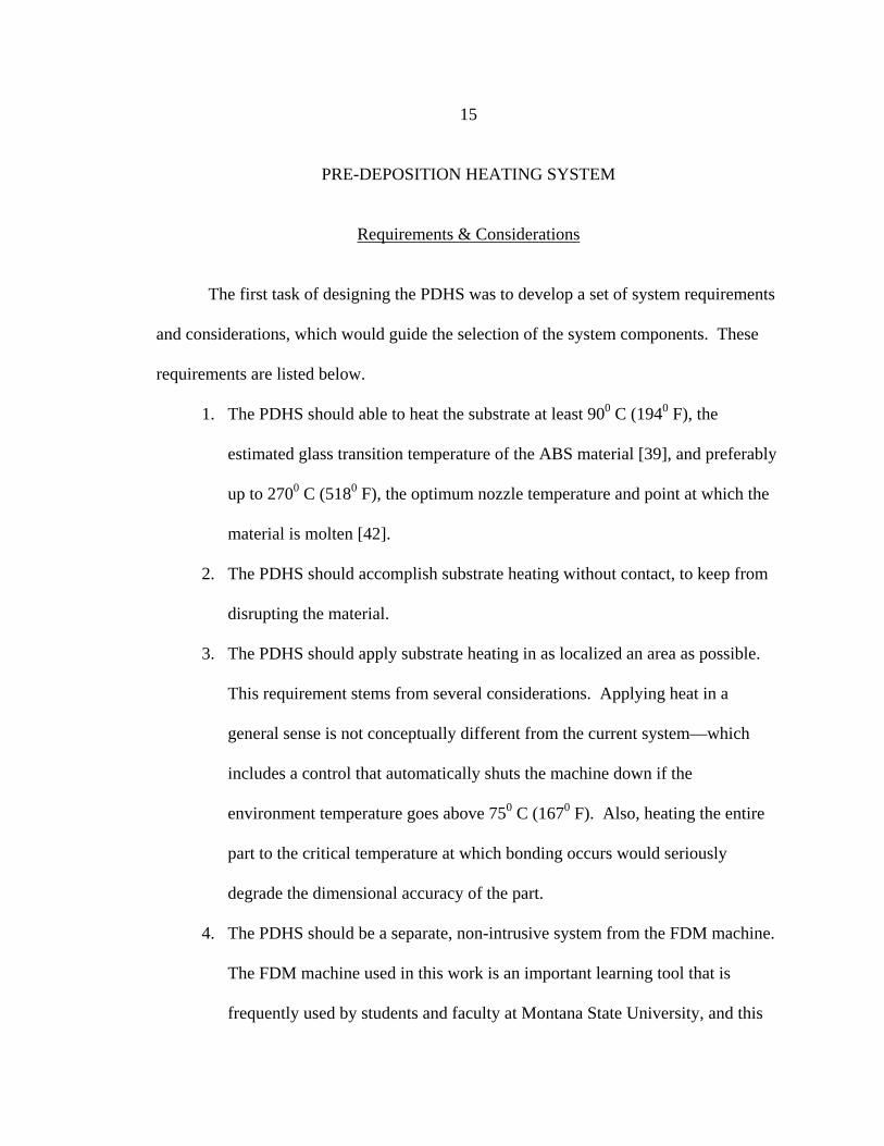
Requirements & Considerations The first task of designing the PDHS was to develop a set of system requirements

and considerations, which would guide the selection of the system components. These

requirements are listed below.

1. The PDHS should able to heat the substrate at least 900 C (1940 F), the

estimated glass transition temperature of the ABS material [39], and preferably

up to 2700 C (5180 F), the optimum nozzle temperature and point at which the

material is molten [42].

2. The PDHS should accomplish substrate heating without contact, to keep from

disrupting the material.

3. The PDHS should apply substrate heating in as localized an area as possible.

This requirement stems from several considerations. Applying heat in a

general sense is not conceptually different from the current system—which

includes a control that automatically shuts the machine down if the

environment temperature goes above 750 C (1670 F). Also, heating the entire

part to the critical temperature at which bonding occurs would seriously

degrade the dimensional accuracy of the part.

4. The PDHS should be a separate, non-intrusive system from the FDM machine.

The FDM machine used in this work is an important learning tool that is

frequently used by students and faculty at Montana State University, and this

16

requirement was out of consideration to those users. Essentially, this

requirement means that the system must be implemented without drilling holes

or otherwise permanently modifying the FDM machine. This work is a proof

of concept, and so the PDHS must be able to be removed from the FDM

machine at its conclusion.

The next section contains a discussion of the technologies that were investigated as the

basis for the PDHS, and how the list of requirements listed above was used to select the

technology for the system.

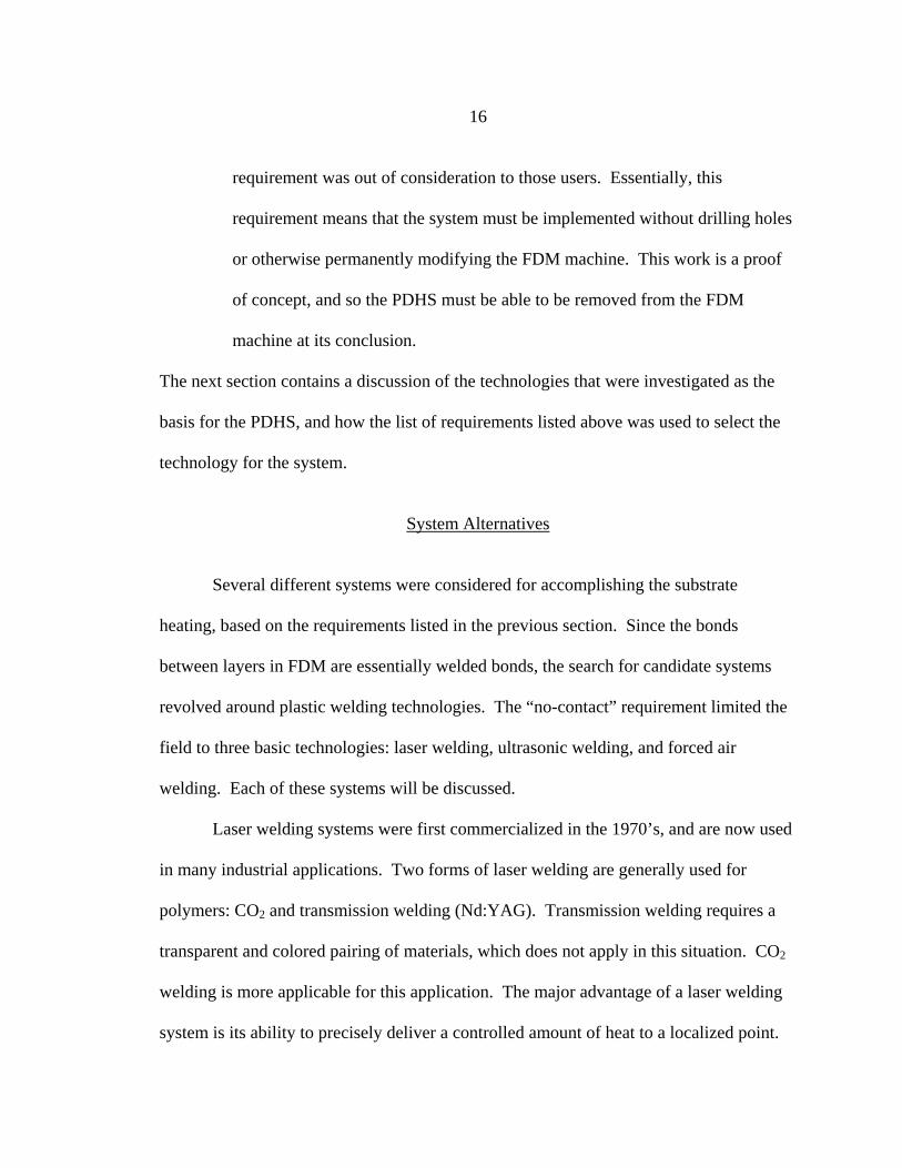
System Alternatives

Several different systems were considered for accomplishing the substrate

heating, based on the requirements listed in the previous section. Since the bonds

between layers in FDM are essentially welded bonds, the search for candidate systems

revolved around plastic welding technologies. The “no-contact” requirement limited the

field to three basic technologies: laser welding, ultrasonic welding, and forced air

welding. Each of these systems will be discussed.

Laser welding systems were first commercialized in the 1970’s, and are now used

in many industrial applications. Two forms of laser welding are generally used for

polymers: CO2 and transmission welding (Nd:YAG). Transmission welding requires a

transparent and colored pairing of materials, which does not apply in this situation. CO2

welding is more applicable for this application. The major advantage of a laser welding

system is its ability to precisely deliver a controlled amount of heat to a localized point.

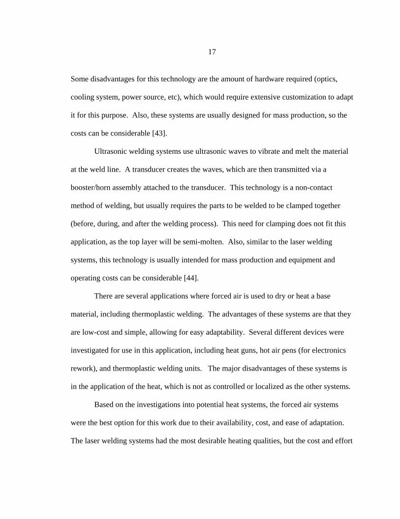
17

Some disadvantages for this technology are the amount of hardware required (optics,

cooling system, power source, etc), which would require extensive customization to adapt

it for this purpose. Also, these systems are usually designed for mass production, so the

costs can be considerable [43].

Ultrasonic welding systems use ultrasonic waves to vibrate and melt the material

at the weld line. A transducer creates the waves, which are then transmitted via a

booster/horn assembly attached to the transducer. This technology is a non-contact

method of welding, but usually requires the parts to be welded to be clamped together

(before, during, and after the welding process). This need for clamping does not fit this

application, as the top layer will be semi-molten. Also, similar to the laser welding

systems, this technology is usually intended for mass production and equipment and

operating costs can be considerable [44].

There are several applications where forced air is used to dry or heat a base

material, including thermoplastic welding. The advantages of these systems are that they

are low-cost and simple, allowing for easy adaptability. Several different devices were

investigated for use in this application, including heat guns, hot air pens (for electronics

rework), and thermoplastic welding units. The major disadvantages of these systems is

in the application of the heat, which is not as controlled or localized as the other systems.

Based on the investigations into potential heat systems, the forced air systems

were the best option for this work due to their availability, cost, and ease of adaptation.

The laser welding systems had the most desirable heating qualities, but the cost and effort

18

of implementation were beyond the scope of this work. The following sections discuss

the development of the system, beginning with the selection of the heating system.

Heating System

As discussed in the previous section, several different types of forced air heater

were investigated. The heat range requirement proved to be a major factor in finding a

suitable heater, as most of the readily available heat guns (for painting applications, etc)

do not heat to 2700 F. Other desirable factors were adjustability of temperature and air

flow, and anticipated ease of integration with the FDM system. The heater selected for

the PDHS system was a PVC welding kit made by Chicago Electric Power Tools© (see

Appendix A for product information). The welder is a hand-held unit that heats

compressed air supplied through a flexible integrated power/air cord specifically

designed to weld thermoplastics.

The manual for the welder lists a maximum temperature of 6000 F (315.50 C),

which satisfies the temperature requirement. However, the welder does not have any

controls that allow the user to adjust the temperature. To address this, a Variac© variable

transformer was obtained and used to regulate the voltage supplied to the welder, which

in turn controls the temperature [45]. In addition, a valve was attached between the

compressed air supply and the welder which allows the user to adjust the air flow.

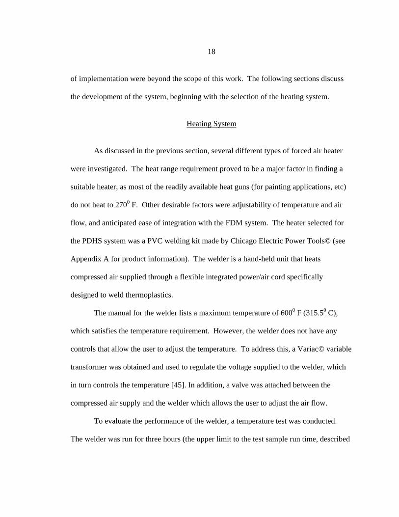
To evaluate the performance of the welder, a temperature test was conducted.

The welder was run for three hours (the upper limit to the test sample run time, described

19

in the next chapter) at full power with the air valve open, with a thermocouple positioned

close to the output nozzle of the welder to measure the air temperature (see Figure 4).

Figure 4. PVC welder temperature test setup

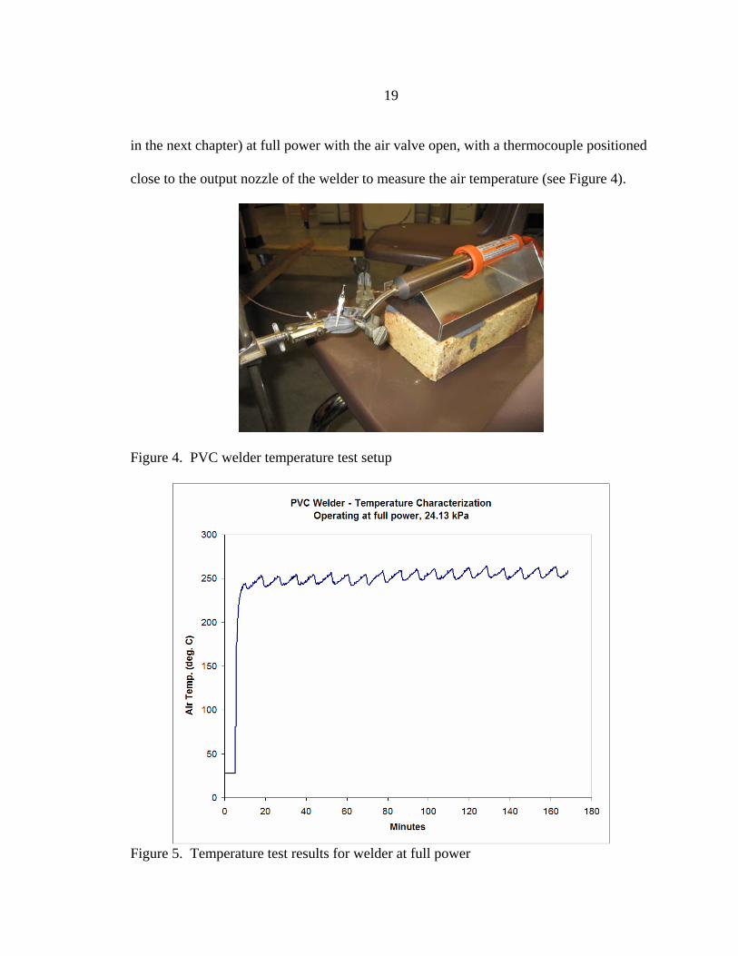
Figure 5. Temperature test results for welder at full power

20

The results of the test showed that after a warm-up time of approximately 10

minutes, the air temperature fluctuates in an approximately periodic way: cycling

approximately every 8 minutes between a maximum temperature of 262.90 C and a

minimum temperature of 240.30 C, with an average temperature of 250.90 C (see Figure

5). The fluctuation is most likely caused by temperature controls in the welder, which

would explain its cyclic nature. The amount of fluctuation in temperature was

disappointing, since it is desirable to keep the temperature as constant as possible. As a

result, for the purposes of the experiment, the voltage will be used as the factor

controlling temperature (since it can be set at a constant level by the user) and it will be

recognized that each voltage produces a range of air temperatures, rather than a single

constant temperature. This temperature resolution is not ideal, but will serve for the

purpose of satisfying the goal of this thesis, which is to investigate the effects of pre-

deposition heating in a general sense (rather than optimizing the air temperature).

Mounting and Heat Delivery Hardware: Welder to the Deposition Head

Once the heating component of the PDHS was selected, the next step was to

develop the hardware for mounting the components in the desired locations and

delivering the heated air to the desired location in front of the nozzle. There are two

stages of heat delivery: delivering the air from the heater to the deposition head, and

delivering the air from the deposition head to the point of application in front of the

material nozzle. The hardware development of each of these stages will be discussed

separately.

21

The initial design of the system was to keep the PVC welder outside of the FDM

enclosure so that it could be monitored easily, and use hose to run the air from the welder

to the deposition head. The hose had to be flexible to allow for free movement of the

deposition head. In addition, the distance from the PVC welder (assuming that it would

be mounted to the back of the FDM) to the deposition head, with enough slack to allow

for the deposition head to reach any point in the enclosure, was measured at 1.54 m (the

best access to the deposition head is through a door on the back of the enclosure). Thus,

the requirements for the hose were flexibility, capability of withstanding air heated to

temperatures in excess of 2700 C, and a 1.54 m length.

After some research, it was determined that the best option for the hose was 0.635

cm 304 SS braided hose, which was the most flexible hose found that was still capable of

handling the high temperatures of air. The nozzle on the PVC welder unscrews, allowing

hose with a 0.635 cm NPT male fitting to be screwed directly to the welder. A 1.54 m

length of the hose with the appropriate fittings was purchased and attached to the PVC

welder. To prevent heat loss, the hose was wrapped with fiberglass insulation tape. The

welder was run at full power for several hours, and the air temperature at the hose outlet

was monitored. However, the temperature of the air never rose above 700 C, which was

deemed unacceptable for this application. The cause for the reduction in air temperature

was most likely due to convective cooling in the hose.

The results of testing the flexible hose led to the conclusion that heater must be as

close to the point of application as possible, to minimize the amount of heat lost during

transit. Therefore, it was decided to mount the PVC welder directly to the deposition

22

head. The cord supplying the power and air to the welder is 3.65 m long and flexible,

easily allowing for deposition head movement. Once this was decided, the next step was

to design a frame for mounting the welder.

The first step in designing the frame to fix the welder to the deposition head was

to determine the mounting location. The diameter of the welder eliminates mounting it to

the underside of the head, as there would be insufficient clearance. Likewise, the rails on

which the head is mounted would obstruct the welder if it was mounted to the top.

Between the two sides, the right side has more hardware and wiring, whereas the left side

is clear except for a buckle, which sticks out about .012 m from the side of the head.

Therefore, it was decided to mount the welder on the left side. An aluminum plate was

cut to the length of the deposition head, and six bolts with aluminum spacers were

mounted around the edges of the frame to allow the frame to clear the buckle on the side.

The next step was to determine both how to rigidly fix the frame onto the

deposition head, and how to locate the frame on the deposition head so that it could be

removed and reattached in the same place. In keeping with the system requirements

listed previously, this had to be accomplished without drilling holes or otherwise

permanently altering the deposition head. In the first iteration of the design, a through

hole found in the section of the deposition head hardware used to mount the head onto the

overhead rails, towards the front of the head. This hole provided a means of both

locating the frame and supporting the frame in the vertical direction: two bolts with

threaded 0.635 cm nylon spacers were mounted to the frame, one to fit into the hole in

the front, the other to rest on the top of the head in the rear.

23

At this point, the frame could rest in position to the deposition head, but was not

securely fastened to it. To accomplish this, some means of strapping the frame onto the

deposition head needed to be added. The first solution was to use a simple bungee cord

to hold the frame firmly against the side of the head. However, during one of the trial

runs of the system, the bungee cord was used to wrap the entire assembly (welder and

frame) to the head, and it pressed too tightly against the rubber grip of the welder. This

caused the grip to come into contact with the heating element, which melted both the

rubber and bungee cord before the system was turned off. The next solution was to use

hook-and-eye strapping material to secure the frame to the head, which has the added

benefit of ease of use in attaching and un-attaching the frame.

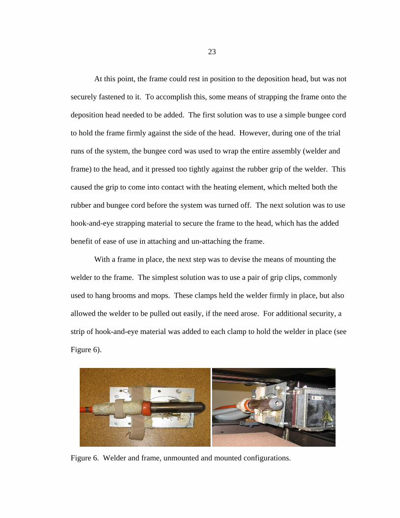
With a frame in place, the next step was to devise the means of mounting the

welder to the frame. The simplest solution was to use a pair of grip clips, commonly

used to hang brooms and mops. These clamps held the welder firmly in place, but also

allowed the welder to be pulled out easily, if the need arose. For additional security, a

strip of hook-and-eye material was added to each clamp to hold the welder in place (see

Figure 6).

Figure 6. Welder and frame, unmounted and mounted configurations.

24

At this point in the design, the welder could be attached to the deposition head

securely. However, there is one aspect of the system that is worth noting. The procedure

for running a part on the FDM begins by “Sending” the part to the machine, at which

point the machine goes through a “homing” procedure—during which the deposition

head travels to the front left corner of the enclosure. After completing this procedure, the

machine pauses, allowing the user to position the deposition head in the desired location

within the enclosure before starting part fabrication. The movement to the corner of the

enclosure during “homing” brings the deposition head to a position where there is not

enough clearance between the side of the enclosure and the welder/frame assembly. This

means that each time a part is run, the user must run the “homing” procedure prior to

attaching the welder/frame assembly for part fabrication. This aspect of the part system

became a key consideration during the next stage of hardware design, as discussed in the

next section.

Mounting and Heat Delivery Hardware: Deposition Head to Substrate

The next stage of heat delivery is to transport the heated air from the welder,

mounted on the side of the deposition head, to the substrate material. Since the

deposition head can move in any direction, a fully functional PDHS should also be able

to heat the substrate in any direction. However, for this work it was decided to restrict

movement of the deposition nozzle to one axis—specifically the x-axis, which runs from

left to right (from the front of the enclosure). This restriction was to simplify the heat

25

delivery requirements, as now the heated air only needs to be applied to the left and to the

right of the material nozzle, rather than all the way around it.

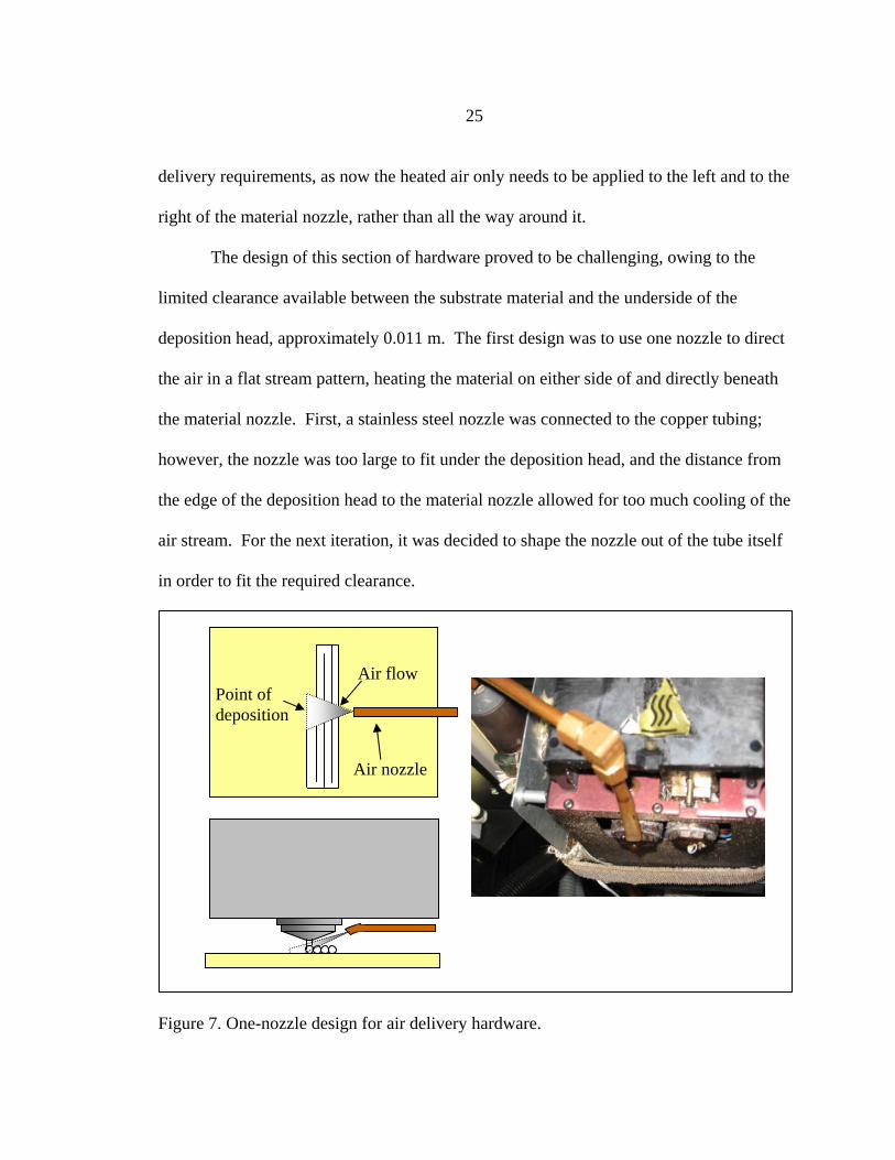
The design of this section of hardware proved to be challenging, owing to the

limited clearance available between the substrate material and the underside of the

deposition head, approximately 0.011 m. The first design was to use one nozzle to direct

the air in a flat stream pattern, heating the material on either side of and directly beneath

the material nozzle. First, a stainless steel nozzle was connected to the copper tubing;

however, the nozzle was too large to fit under the deposition head, and the distance from

the edge of the deposition head to the material nozzle allowed for too much cooling of the

air stream. For the next iteration, it was decided to shape the nozzle out of the tube itself

in order to fit the required clearance.

Figure 7. One-nozzle design for air delivery hardware.

Point of deposition

Air nozzle

Air flow

26

The next design iteration used straight pieces of copper tubing with elbow fittings

to bring the air into position in front of the nozzle, and a piece of copper tubing to bring

the air as close to the nozzle as possible. This piece was flattened slightly for better

clearance, and the end was shaped to direct the air in a flat spray, angled slightly

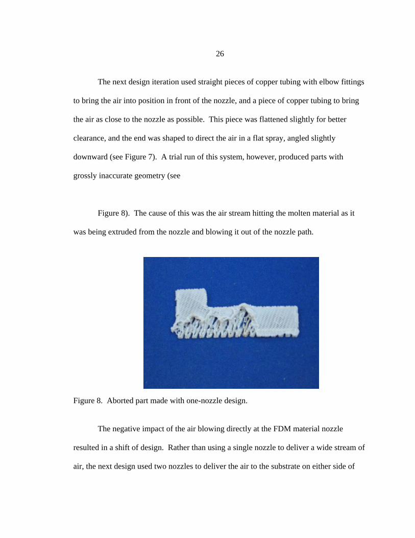
downward (see Figure 7). A trial run of this system, however, produced parts with

grossly inaccurate geometry (see

Figure 8). The cause of this was the air stream hitting the molten material as it

was being extruded from the nozzle and blowing it out of the nozzle path.

Figure 8. Aborted part made with one-nozzle design.

The negative impact of the air blowing directly at the FDM material nozzle

resulted in a shift of design. Rather than using a single nozzle to deliver a wide stream of

air, the next design used two nozzles to deliver the air to the substrate on either side of

27

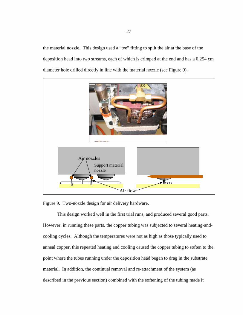
the material nozzle. This design used a “tee” fitting to split the air at the base of the

deposition head into two streams, each of which is crimped at the end and has a 0.254 cm

diameter hole drilled directly in line with the material nozzle (see Figure 9).

Figure 9. Two-nozzle design for air delivery hardware.

This design worked well in the first trial runs, and produced several good parts.

However, in running these parts, the copper tubing was subjected to several heating-and-

cooling cycles. Although the temperatures were not as high as those typically used to

anneal copper, this repeated heating and cooling caused the copper tubing to soften to the

point where the tubes running under the deposition head began to drag in the substrate

material. In addition, the continual removal and re-attachment of the system (as

described in the previous section) combined with the softening of the tubing made it

Support material nozzle

Air nozzles

Air flow

28

difficult to keep the air holes aligned properly with the FDM material nozzle. The loss of

rigidity and alignment issues with the copper tubing fixture led to the next design

iteration. In this design, a length of copper tubing connects the welder to a machined

aluminum block, which is clamped onto a plastic component on the front of the

deposition head. The block has been machined to channel the air into two 0.317 cm brass

tubes, which deliver the air to the substrate in a similar manner as the previous design:

each tube is crimped at the end and has a 0.127 cm diameter hole drilled in line with the

deposition head. This design has several advantages over previous designs. The support

from clamping the aluminum plate to the FDM deposition head provides much better

support and rigidity than the previous systems, which relied on the stiffness of the copper

tubing to maintain necessary clearances and positioning. In addition, clamping the

aluminum block to the head allows for permanent placement of the air stream, since the

welder/frame assembly can be easily attached or unattached by screwing or unscrewing

the copper tubing fitting in the aluminum block (and the aluminum block does not have

clearance issues during the “homing” procedure). This allows for much better

consistency in keeping the air holes aligned with the model material nozzle than previous

designs.

Once the system was in place, the placement of the air flow was adjusted. First, it

was important to ensure that the air flows were properly aligned with the nozzle. Second,

the air stream needed to be as close to the material nozzle as possible—but not to the

point where the air disturbed material deposition. In order to determine where the air

stream was hitting relative to the nozzle, a folded strip of paper with heat-sensitive ink

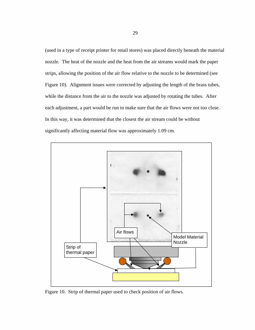
29

(used in a type of receipt printer for retail stores) was placed directly beneath the material

nozzle. The heat of the nozzle and the heat from the air streams would mark the paper

strips, allowing the position of the air flow relative to the nozzle to be determined (see

Figure 10). Alignment issues were corrected by adjusting the length of the brass tubes,

while the distance from the air to the nozzle was adjusted by rotating the tubes. After

each adjustment, a part would be run to make sure that the air flows were not too close.

In this way, it was determined that the closest the air stream could be without

significantly affecting material flow was approximately 1.09 cm.

Figure 10. Strip of thermal paper used to check position of air flows.

Strip of thermal paper

Air flowsModel Material Nozzle

30

The final component to making parts was determining where to set the envelope

temperature. As mentioned in the introduction, this temperature is maintained by a heater

and fan system, and the envelope temperature setting recommended by Stratasys for this

material is 700 C. However, an issue with the temperature control system of the FDM

made using the envelope temperature infeasible. In practice it is not uncommon for the

machine to shut down if the door is left open too long when the envelope temperature is

set to 700 C. The reason for this is that the open door causes the envelope temperature to

drop, causing the heater to switch on to return the temperature to the specified setting; the

heater causes the temperature to rise so fast that it continues rising, even after the

specified temperature is reached and the fans turn on. This overcorrection does not

usually cause a problem, unless it takes the envelope temperature above the maximum

temperature allowed by the FDM machine, 750 C, in which case the machine

automatically shuts off. During the development of the PDHS, it became apparent that

additional heat put out by the PDHS was more than the fan controlling the envelope

temperature could handle. As a result, it became necessary to prop the door open slightly

in order for the FDM to maintain a somewhat constant envelope temperature. However,

this and the additional air flow circulating in the FDM cause there to be a greater

fluctuation in the envelope temperature than usual. With this amount of fluctuation in

mind, the envelope temperature for PDHS parts was set to 650 C to avoid surpassing the

maximum allowable temperature.

31

EXPERIMENTAL DESIGN An experiment was needed in order to measure the effects of the pre-deposition

heating system (PDHS) discussed in the previous chapter. This chapter discusses the

design and procedures of this experiment, beginning with the design of the test part used

to measure the variables of interest, followed by a brief discussion of the statistical

principles used to analyze the experimental data. The chapter ends with the development

of the experimental design used in this work.

Test Part Design

As described in the Introduction, the goal of the PDHS is to improve part

interlayer strength without negatively impacting the material properties or dimensional

accuracy. Therefore, the test part used to in the experiment was designed to allow for

measurements of interlayer strength, road tensile strength (to test for material

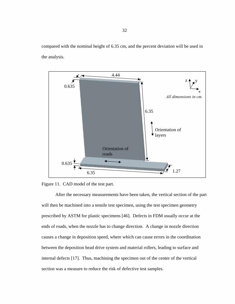
degradation), and dimensional accuracy. The test part design is shown in Figure 11.

The vertical section of the part provides data for interlayer strength and

dimensional accuracy. As the major concern regarding dimensional accuracy is that the

part may slump due to the additional heating (damaging the dimensional accuracy in the

vertical direction), the height of the vertical section will be measured in each part to

detect any changes in dimensional accuracy. Three measurements will be taken from the

vertical section: 0.635 cm from either side and in the middle. The average height will be

32

compared with the nominal height of 6.35 cm, and the percent deviation will be used in

the analysis.

Figure 11. CAD model of the test part.

After the necessary measurements have been taken, the vertical section of the part

will then be machined into a tensile test specimen, using the test specimen geometry

prescribed by ASTM for plastic specimens [46]. Defects in FDM usually occur at the

ends of roads, when the nozzle has to change direction. A change in nozzle direction

causes a change in deposition speed, where which can cause errors in the coordination

between the deposition head drive system and material rollers, leading to surface and

internal defects [17]. Thus, machining the specimen out of the center of the vertical

section was a measure to reduce the risk of defective test samples.

1.27 6.35

0.635

Orientation of roads

6.35

0.635

4.44

All dimensions in cm.

Orientation of layers

x

yz

33

The flat section of the part was designed to measure the axial strength of the part.

The roads for this section were specified in QuickSlice© to run along the length of the

part, so that a test specimen from this section would test the strength of the roads

themselves. The purpose of this test was to check for degradation of material properties

due to overheating of the material.

Analysis of Variance (ANOVA)

Analysis of Variance (ANOVA) is the term given to a type of statistical analysis

used to detect changes of some response variable in a group of samples, usually due to

user-controlled changes in one or more sample treatments. The foundation of ANOVA is

statistical hypothesis testing, where a null hypothesis is tested against an alternate

hypothesis based on a level of significance. In ANOVA, the null hypothesis is that the

means of all of the sample groups—that is, groups of sample produced at each level of

each treatment—are the same. The comparison between groups is made by splitting the

total sum of square, a measure of deviation from the overall mean, into two components:

deviation due to the treatment differences, and deviation due to error or variation within a

sample group. The sums of squares due to these potential sources of variation are

converted into mean squares, which allows for a test for statistical significance using

Fisher’s F-distribution, based on a user-selected level of significance [47].

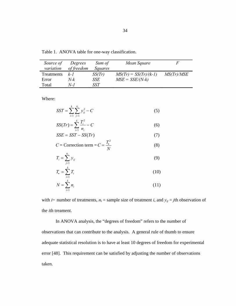
The results obtained using ANOVA are usually summarized in an ANOVA table, as

shown below in

Table 1.

34

Table 1. ANOVA table for one-way classification.

Source of variation

Degrees of freedom

Sum of Squares

Mean Square F

Treatments k-1 SS(Tr) MS(Tr) = SS(Tr)/(k-1) MS(Tr)/MSE Error N-k SSE MSE = SSE/(N-k) Total N-1 SST

Where:

SST y Cijj

n

i

k i

= −==∑∑ 2

11

(5)

SS Tr Tn

Ci

ii

k

( ) = −=∑

2

1

(6)

SSE SST SS Tr= − ( ) (7)

C = Correction term = C TN

= •2

(8)

T yi ijj

ni

==∑

1

(9)

T Tii

k

•=

= ∑1

(10)

N nii

k

==∑

1

(11)

with i= number of treatments, ni = sample size of treatment i, and yij = jth observation of

the ith treament.

In ANOVA analysis, the “degrees of freedom” refers to the number of

observations that can contribute to the analysis. A general rule of thumb to ensure

adequate statistical resolution is to have at least 10 degrees of freedom for experimental

error [48]. This requirement can be satisfied by adjusting the number of observations

taken.

35

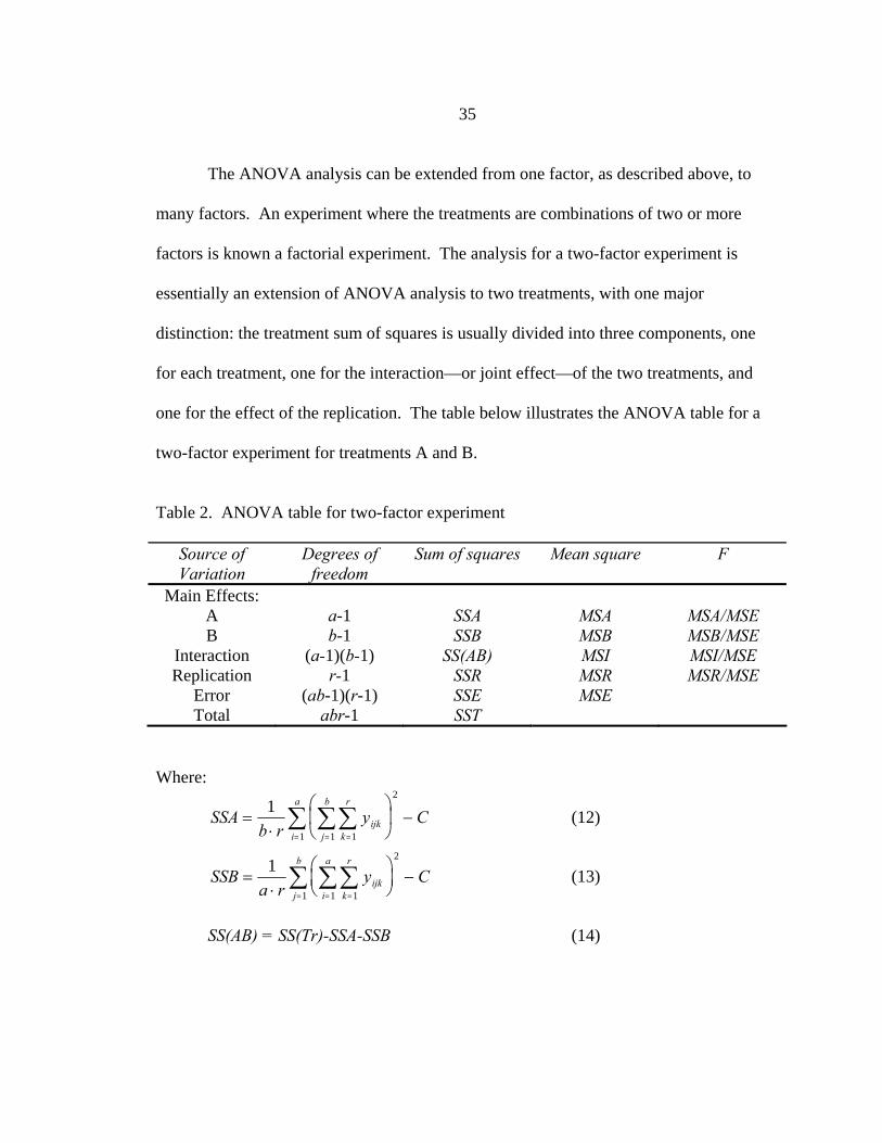
The ANOVA analysis can be extended from one factor, as described above, to

many factors. An experiment where the treatments are combinations of two or more

factors is known a factorial experiment. The analysis for a two-factor experiment is

essentially an extension of ANOVA analysis to two treatments, with one major

distinction: the treatment sum of squares is usually divided into three components, one

for each treatment, one for the interaction—or joint effect—of the two treatments, and

one for the effect of the replication. The table below illustrates the ANOVA table for a

two-factor experiment for treatments A and B.

Table 2. ANOVA table for two-factor experiment

Source of Variation

Degrees of freedom

Sum of squares Mean square F

Main Effects: A B

a-1 b-1

SSA SSB

MSA MSB

MSA/MSE MSB/MSE

Interaction (a-1)(b-1) SS(AB) MSI MSI/MSE Replication r-1 SSR MSR MSR/MSE

Error (ab-1)(r-1) SSE MSE Total abr-1 SST

Where:

SSAb r

y Cijkk

r

j

b

i

a

=⋅

⎛

⎝⎜

⎞

⎠⎟ −

===∑∑∑1

11

2

1

(12)

SSBa r

y Cijkk

r

i

a

j

b

=⋅

⎛⎝⎜

⎞⎠⎟ −

===∑∑∑1

11

2

1

(13)

SS(AB) = SS(Tr)-SSA-SSB (14)

36

SS Try

r

ijkk

r

j

b

i

a

( ) =

⎛⎝⎜

⎞⎠⎟

===∑∑∑

1

2

11 (15)

SSRy

ab

ijkj

b

i

a

k

r

=

⎛

⎝⎜

⎞

⎠⎟

===∑∑∑

11

2

1 (16)

SSE = SST-SS(Tr)-SSR (17)

SST y Cijkk

r

j

b

i

a

= −===∑∑∑ 2

111

(18)

Cy

abr

ijkk

r

j

b

i

a

=

⎛

⎝⎜

⎞

⎠⎟

===∑∑∑

111

2

(19)

with a = number of levels of A, b = number of levels of B, and r = number of

replications.

The ANOVA analysis detects whether the treatment effects account for a

significant difference in the response variable. However, it is usually useful to quantify

the amount of difference in some way. One method of doing this is the Duncan multiple-

range test, which compares the range of a set of p means to a variable known as the least

significant range, Rp, defined by:

R s rp y p= ⋅ (20)

Where

s MSEny = (21)

37

and rp is the critical value for the number of means, p, associated with the chosen level of

significance and the number of degrees of freedom corresponding to MSE. Values for rp

have been tabulated and are available in many statistics handbooks; the values in this

work are from Miller and Freund [49]. The procedure for using the Duncan multiple-

range test is to order the sample means, calculate the ranges for a given value of p, and

compare those ranges with the values of Rp. A range of sample means that is greater than

its corresponding value of Rp indicates a significant difference between the means. The

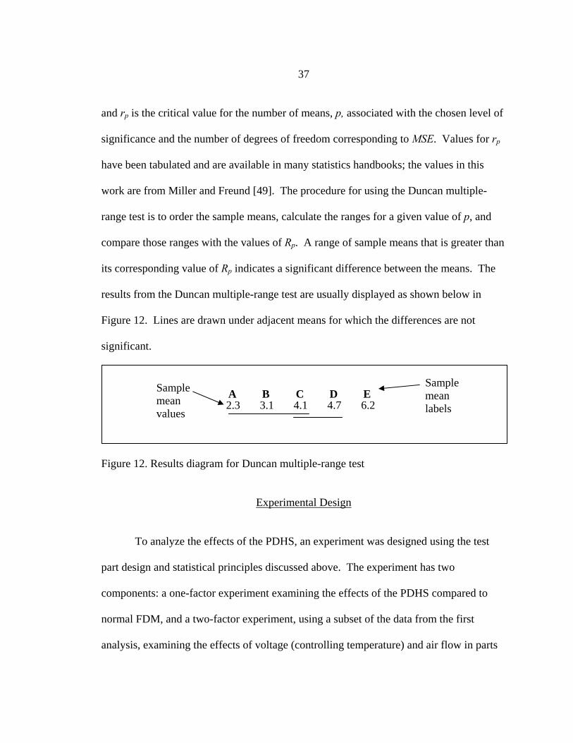
results from the Duncan multiple-range test are usually displayed as shown below in

Figure 12. Lines are drawn under adjacent means for which the differences are not

significant.

Figure 12. Results diagram for Duncan multiple-range test

Experimental Design

To analyze the effects of the PDHS, an experiment was designed using the test

part design and statistical principles discussed above. The experiment has two

components: a one-factor experiment examining the effects of the PDHS compared to

normal FDM, and a two-factor experiment, using a subset of the data from the first

analysis, examining the effects of voltage (controlling temperature) and air flow in parts

A B C D E2.3 3.1 4.1 4.7 6.2

Sample mean values

Sample mean labels

38

made using the PDHS. The “treatment” of the one-factor analysis is the environmental

heating method (non-PDHS vs. PDHS) at several different levels, including parts made at

different voltages and air flow levels with the PDHS. The data from the parts made using

the PDHS will then be examined using a two-factor analysis to investigate the effects of

the PDHS temperature and air flow. The first step in the experimental design was to

select the treatment levels of each factor.

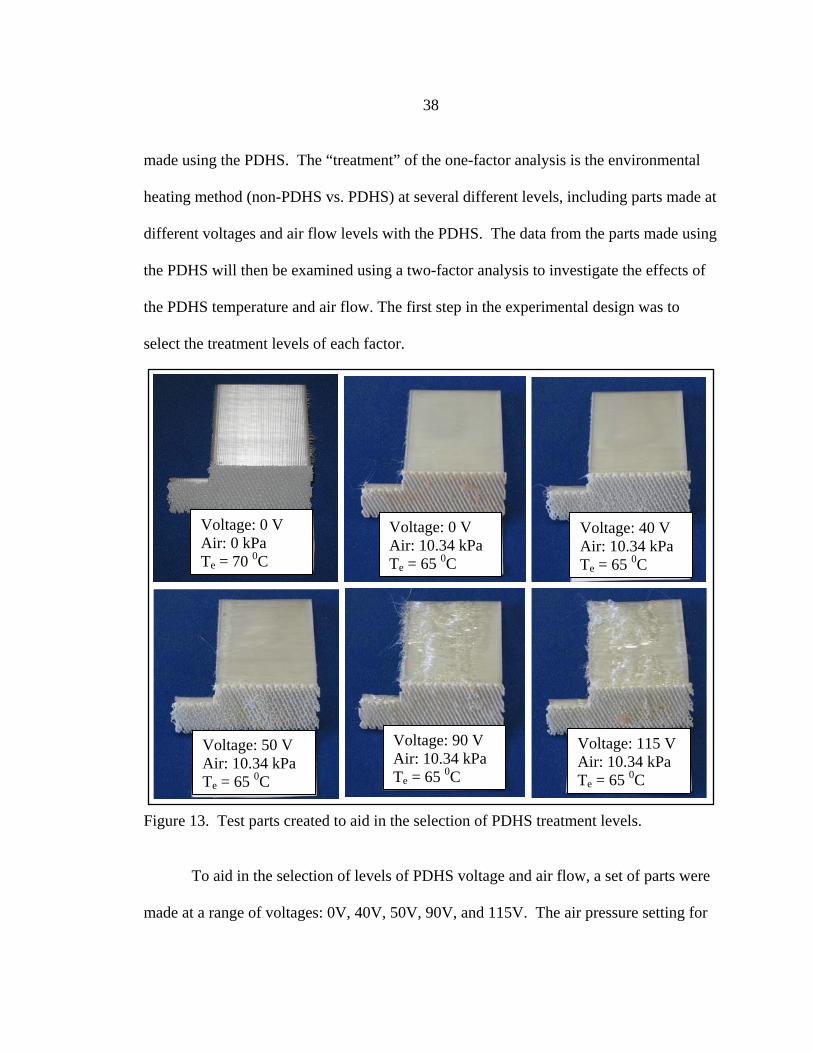
Figure 13. Test parts created to aid in the selection of PDHS treatment levels.

To aid in the selection of levels of PDHS voltage and air flow, a set of parts were

made at a range of voltages: 0V, 40V, 50V, 90V, and 115V. The air pressure setting for

Voltage: 0 V Air: 0 kPa Te = 70 0C

Voltage: 0 V Air: 10.34 kPa Te = 65 0C

Voltage: 40 V Air: 10.34 kPa Te = 65 0C

Voltage: 50 V Air: 10.34 kPa Te = 65 0C

Voltage: 90 V Air: 10.34 kPa Te = 65 0C

Voltage: 115 V Air: 10.34 kPa Te = 65 0C

39

these samples was set at 10.34 kPa (1.5 psi), which was the lowest pressure that the flow

switch was able to maintain. As discussed in the previous chapter, the envelope

temperature was set to 650 C. Images of these samples are shown below in Figure 13.

The images show how the surface finish degrades as the temperature of the PDHS

increases. Parts made at 50 V and higher showed increasingly severe waviness of the

roads on the side surfaces of the upright section of the test part. Parts made at 40 V or

below showed little or no waviness of the surface layer. This waviness of the surface

layer of roads appears to be due to a combination of heat and air flow, at higher

temperatures, the material stays softer and is more easily disturbed by the air flow.

The roads on the surface are the first roads to be deposited on each layer, so they

are especially prone to this disturbance, as they are only supported from the bottom—

where internal roads are supported from the bottom and from the side of the previous

road. While this loss in geometric accuracy is not desirable, it was decided to include the

higher temperatures in the experiment to see if there was an increase in interlayer

strength.

Another note of interest is that during fabrication of the parts at the highest

voltage (115 V), the PVC welder overheated and had to be replaced. To avoid this in the

experiment, it was decided to set the maximum voltage setting of the PVC welder to 90

V. Based on this consideration and the pilot study, four voltage levels were selected for

the experiment: 0 V (air only), 40 V, 65 V, and 90 V. To examine how the amount of air

flow affected the process, two levels were chosen for the air pressure: 10.34 kPa and

40

20.68 kPa. These values of PDHS voltage and air pressure comprise the levels of the

two-factor experiment, making it a 4 x 2 factorial experiment.

The goal of the one-factor analysis was to compare parts fabricated using the

PDHS with those made without it. Therefore, it was necessary that at least one level of

treatment would be parts made without the PDHS. Without the PDHS, the remaining

environmental parameter is the envelope temperature. Two levels were selected for non-

PDHS parts: one level with an envelope temperature of 700 C and one level at an

envelope temperature at 650 C. The level at 650 C was chosen to match the envelope

temperature selected for the PDHS parts, which allows for comparison between parts

made with and without the PDHS with all other parameters being the same.

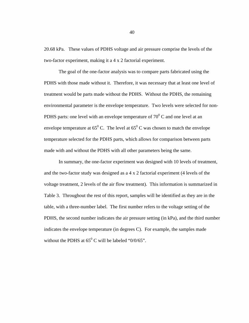
In summary, the one-factor experiment was designed with 10 levels of treatment,

and the two-factor study was designed as a 4 x 2 factorial experiment (4 levels of the

voltage treatment, 2 levels of the air flow treatment). This information is summarized in

Table 3. Throughout the rest of this report, samples will be identified as they are in the

table, with a three-number label. The first number refers to the voltage setting of the

PDHS, the second number indicates the air pressure setting (in kPa), and the third number

indicates the envelope temperature (in degrees C). For example, the samples made

without the PDHS at 650 C will be labeled “0/0/65”.

41

Table 3. Description of the experiment treatment levels

Analysis Treatment Levels One-factor experiment Environmental Heating

__V/___kPa/___0C 1. 0/0/65 2. 0/0/70 3. 0/10.34/65 4. 0/20.68/65 5. 40/10.34/65 6. 40/20.68/65 7. 65/10.34/65 8. 65/20.68/65 9. 90/10.34/65 10. 90/20.68/65

PDHS Voltage 1. 0V 2. 40V 3. 65V 4. 90V

Two-factor experiment

PDHS Air pressure 1. 10.34 kPa 2. 20.68 kPa

The next component of experimental design was to set the sample size. As

mentioned in the ANOVA background section, a general rule of thumb is to set the

sample size for each treatment so that the error degrees of freedom are greater than 10.

With this rule of thumb in mind, the sample size was set at five samples per treatment

level, or five replications (where one replication is one sample of each treatment). This

gives 40 error degrees of freedom for the one-factor analysis and 28 error degrees of

freedom for the two-factor analysis. In addition to satisfying the requirements for error

degrees of freedom this sample size is in line with most ASTM standards, which specify

a minimum sample size of five [46].

42

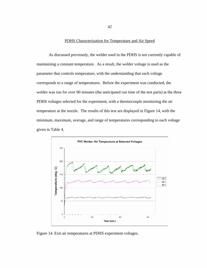
PDHS Characterization for Temperature and Air Speed As discussed previously, the welder used in the PDHS is not currently capable of

maintaining a constant temperature. As a result, the welder voltage is used as the

parameter that controls temperature, with the understanding that each voltage

corresponds to a range of temperatures. Before the experiment was conducted, the

welder was run for over 90 minutes (the anticipated run time of the test parts) at the three

PDHS voltages selected for the experiment, with a thermocouple monitoring the air

temperature at the nozzle. The results of this test are displayed in Figure 14, with the

minimum, maximum, average, and range of temperatures corresponding to each voltage

given in Table 4.

Figure 14. Exit air temperatures at PDHS experiment voltages.

43

Table 4. Temperature statistics for PDHS experiment voltages (excluding 10 min. warm-up)

PDHS Voltage: 40 V 65 V 90 V Minimum Temp. (0C) 60.83 119.16 153.16 Maximum Temp. (0C) 65.61 129.0 197.88 Average Temp. (0C) 63.27 123.66 170.61 Temperature Range (0C) 4.78 9.84 44.72

The results from the temperature characterization show that the range of temperatures

increases dramatically with the voltage. The amount of fluctuation in the 90V case is

especially disappointing; however, since this work is a proof of concept and the range of

temperatures corresponding to each of the voltages do not overlap, this variation was

deemed acceptable for the experiment.

The exit air flow rate of the PDHS was calculated using the continuity equation

and Bernoulli’s equation [50]. The flow rates for each voltage are given in Table 5, and

the analysis is contained in Appendix C.

Table 5. Exit air flow rates Pressure (kPa) Flow Rate (m3/s)

10.34 5.72x10-5

20.68 8.03x10-5

Fabrication & Test Procedure

Test parts were modeled using Pro-Engineer Wildfire© software, and fabricated

using a Stratasys FDM 1650 from P500 MABS feedstock material. This material is the

medical grade of ABS plastic produced by Stratasys Corporation. In keeping with

statistical principles, the order of production was randomized within replications using

the random number generator in Microsoft Excel©. With the exception of the envelope

44

temperature, the FDM processing parameters were set as recommended by Stratasys

Corporation for this material (see Appendix A).

Following deposition, the support material base was removed and the vertical

section of the sample part was measured in three locations to provide data for the

dimensional accuracy of the part. Following the basic procedure used by Grimm [15],

dimensional accuracy was quantified by measuring the height of the vertical section three

places (.635 cm from each end and in the center) and calculating the percent deviation of

the average of these heights from the nominal value (6.35 cm). The reason the vertical

dimension was selected for this data was that dimensional errors would additively cause

deviation from the nominal dimension—in other words, the vertical dimension captures

the entire deposition history.

Once the dimensional data is taken, the vertical and flat sections of the test part

were separated by hand, and prepped for machining by lightly running a file over the

surfaces to provide a level surface for proper seating in the fixture.

Test specimens were machined using a Haas CNC Mill. Coolant was used to

minimize the risk of damaging the parts, which meant that the test specimens were

somewhat damp after machining. They were dried off manually using paper towels, and

then placed in the FDM enclosure (with the envelope temperature at 650 C) for twenty-

four hours as a way of removing excess moisture. It is worth noting that the main focus

of the experiment was comparing the data between samples rather than finding definitive

values (e.g. for a properties database), and so having samples that were completely dry

was not necessary. All samples were machined, stored, and tested together, so it is

45

unlikely that differences in part strength could be attributed to variability in processing,

temperature, or humidity (moisture).

Tensile tests were performed using a model 3343 Instron machine, at a rate of 1

cm/min. Prior to testing, the cross-sectional area and gage length of each specimen was

measured, and used to calculate engineering stress and strain of the sample. This method

of calculating stress treats the part as a homogenous material, and does not reflect the

actual stress on the ABS material itself. This assumption and method is the same as the

procedure used by Han et al. and Bellini et al to calculate strength in FDM parts [34,27].

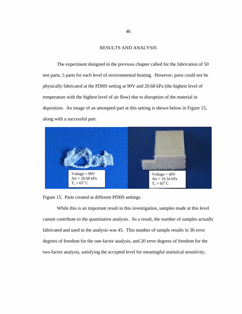
46

RESULTS AND ANALYSIS

The experiment designed in the previous chapter called for the fabrication of 50

test parts, 5 parts for each level of environmental heating. However, parts could not be

physically fabricated at the PDHS setting at 90V and 20.68 kPa (the highest level of

temperature with the highest level of air flow) due to disruption of the material in

deposition. An image of an attempted part at this setting is shown below in Figure 15,

along with a successful part.

Figure 15. Parts created at different PDHS settings.

While this is an important result in this investigation, samples made at this level

cannot contribute to the quantitative analysis. As a result, the number of samples actually

fabricated and used in the analysis was 45. This number of sample results in 36 error

degrees of freedom for the one-factor analysis, and 20 error degrees of freedom for the

two-factor analysis, satisfying the accepted level for meaningful statistical sensitivity.

Voltage = 40V Air = 10.34 kPa Te = 650 C

Voltage = 90V Air = 20.68 kPa Te = 650 C

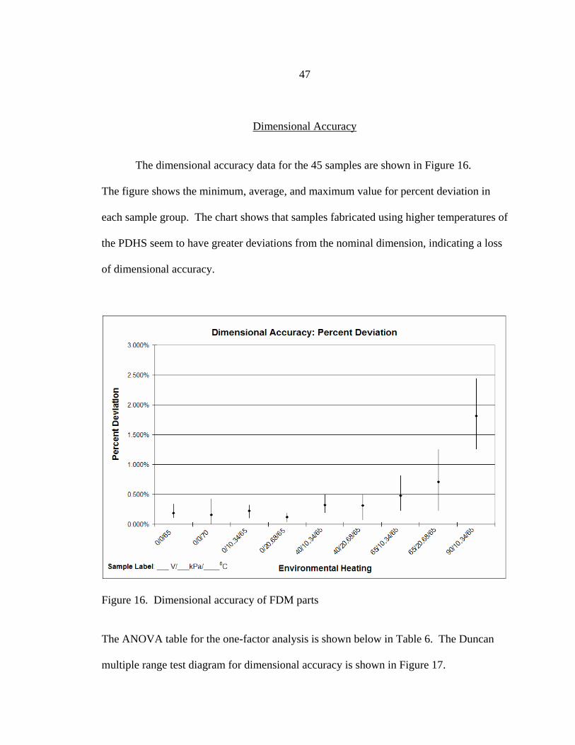
47

Dimensional Accuracy

The dimensional accuracy data for the 45 samples are shown in Figure 16.

The figure shows the minimum, average, and maximum value for percent deviation in

each sample group. The chart shows that samples fabricated using higher temperatures of

the PDHS seem to have greater deviations from the nominal dimension, indicating a loss

of dimensional accuracy.

Figure 16. Dimensional accuracy of FDM parts

The ANOVA table for the one-factor analysis is shown below in Table 6. The Duncan

multiple range test diagram for dimensional accuracy is shown in Figure 17.

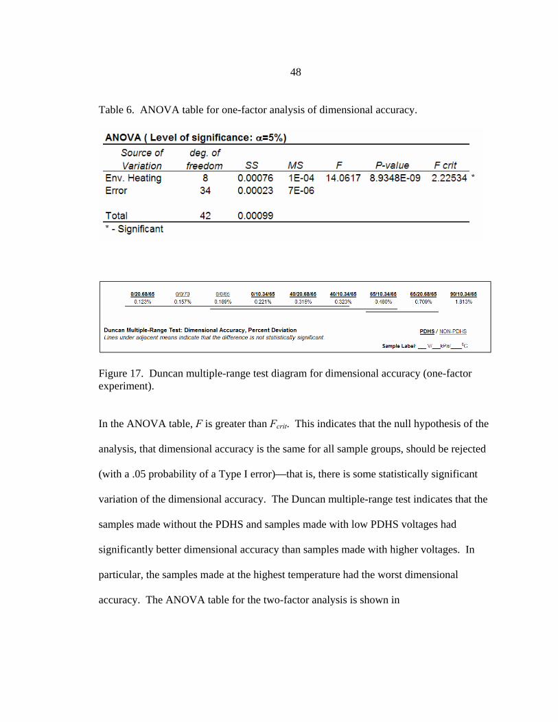
48

Table 6. ANOVA table for one-factor analysis of dimensional accuracy.

Figure 17. Duncan multiple-range test diagram for dimensional accuracy (one-factor experiment).

In the ANOVA table, F is greater than Fcrit. This indicates that the null hypothesis of the

analysis, that dimensional accuracy is the same for all sample groups, should be rejected

(with a .05 probability of a Type I error)—that is, there is some statistically significant

variation of the dimensional accuracy. The Duncan multiple-range test indicates that the

samples made without the PDHS and samples made with low PDHS voltages had

significantly better dimensional accuracy than samples made with higher voltages. In

particular, the samples made at the highest temperature had the worst dimensional

accuracy. The ANOVA table for the two-factor analysis is shown in

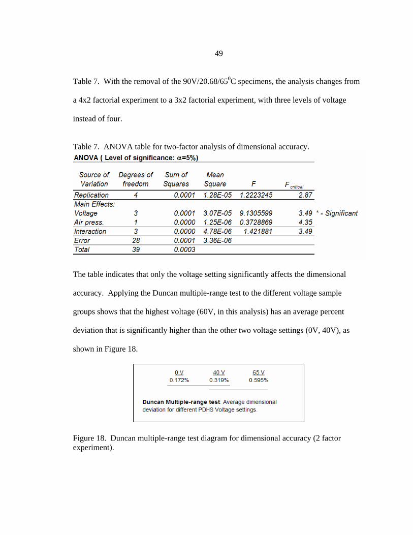
49

Table 7. With the removal of the 90V/20.68/650C specimens, the analysis changes from

a 4x2 factorial experiment to a 3x2 factorial experiment, with three levels of voltage

instead of four.

Table 7. ANOVA table for two-factor analysis of dimensional accuracy.

The table indicates that only the voltage setting significantly affects the dimensional

accuracy. Applying the Duncan multiple-range test to the different voltage sample

groups shows that the highest voltage (60V, in this analysis) has an average percent

deviation that is significantly higher than the other two voltage settings (0V, 40V), as

shown in Figure 18.

Figure 18. Duncan multiple-range test diagram for dimensional accuracy (2 factor experiment).

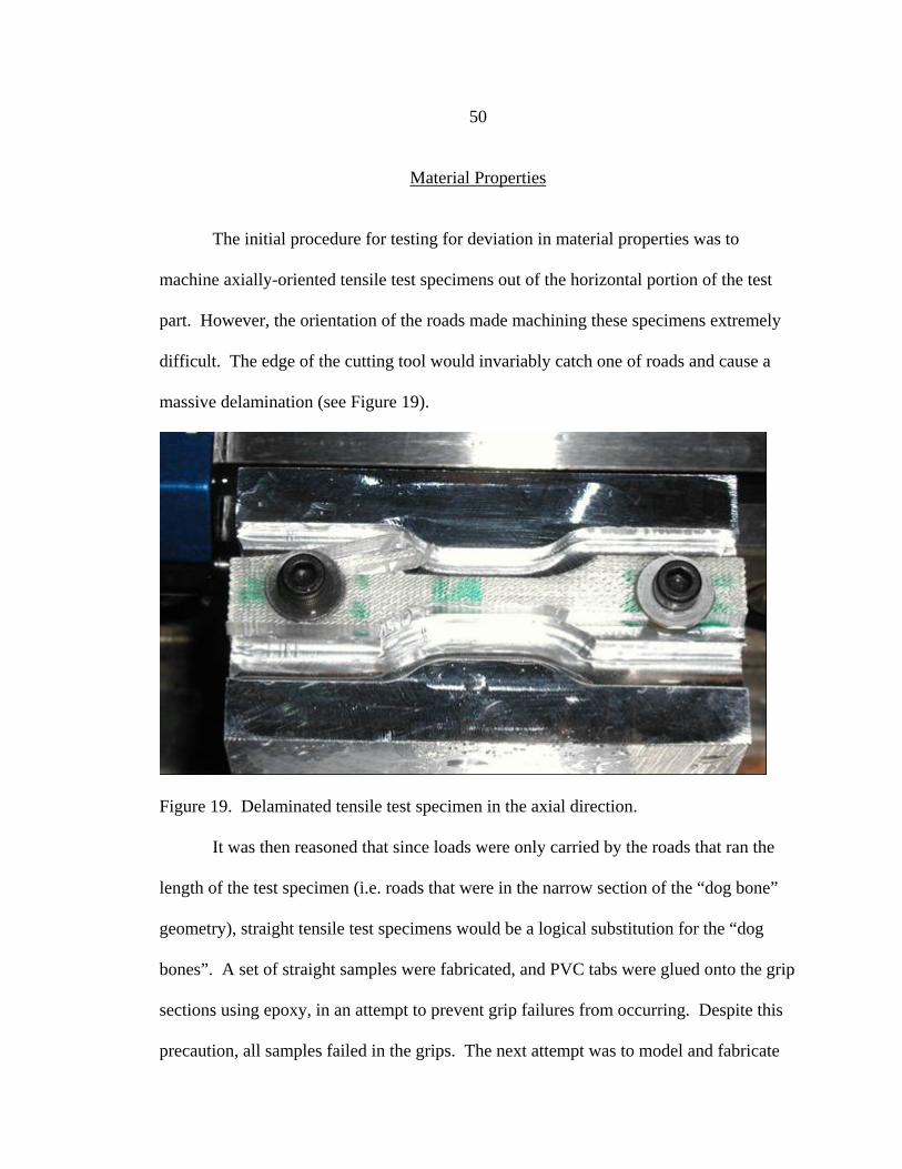
50

Material Properties The initial procedure for testing for deviation in material properties was to

machine axially-oriented tensile test specimens out of the horizontal portion of the test

part. However, the orientation of the roads made machining these specimens extremely

difficult. The edge of the cutting tool would invariably catch one of roads and cause a

massive delamination (see Figure 19).

Figure 19. Delaminated tensile test specimen in the axial direction.

It was then reasoned that since loads were only carried by the roads that ran the

length of the test specimen (i.e. roads that were in the narrow section of the “dog bone”

geometry), straight tensile test specimens would be a logical substitution for the “dog

bones”. A set of straight samples were fabricated, and PVC tabs were glued onto the grip

sections using epoxy, in an attempt to prevent grip failures from occurring. Despite this

precaution, all samples failed in the grips. The next attempt was to model and fabricate

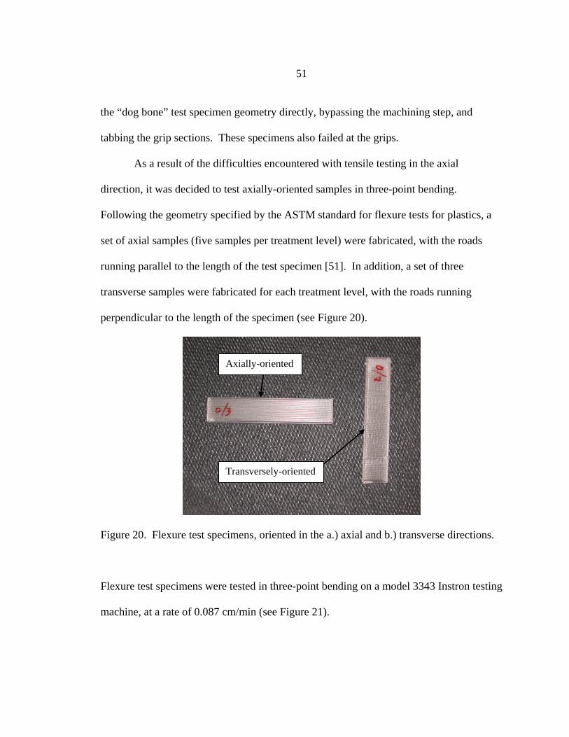
51

the “dog bone” test specimen geometry directly, bypassing the machining step, and

tabbing the grip sections. These specimens also failed at the grips.

As a result of the difficulties encountered with tensile testing in the axial

direction, it was decided to test axially-oriented samples in three-point bending.

Following the geometry specified by the ASTM standard for flexure tests for plastics, a

set of axial samples (five samples per treatment level) were fabricated, with the roads

running parallel to the length of the test specimen [51]. In addition, a set of three

transverse samples were fabricated for each treatment level, with the roads running

perpendicular to the length of the specimen (see Figure 20).

Figure 20. Flexure test specimens, oriented in the a.) axial and b.) transverse directions.

Flexure test specimens were tested in three-point bending on a model 3343 Instron testing

machine, at a rate of 0.087 cm/min (see Figure 21).

Axially-oriented

Transversely-oriented

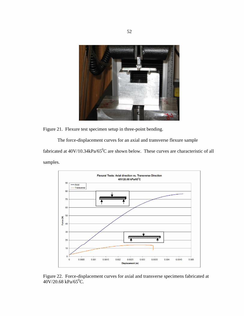
52

Figure 21. Flexure test specimen setup in three-point bending.

The force-displacement curves for an axial and transverse flexure sample

fabricated at 40V/10.34kPa/650C are shown below. These curves are characteristic of all

samples.

Figure 22. Force-displacement curves for axial and transverse specimens fabricated at 40V/20.68 kPa/650C.

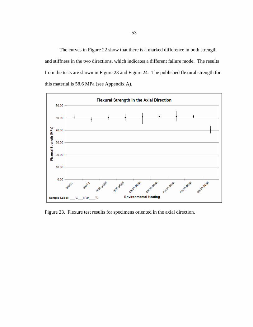
53

The curves in Figure 22 show that there is a marked difference in both strength

and stiffness in the two directions, which indicates a different failure mode. The results

from the tests are shown in Figure 23 and Figure 24. The published flexural strength for

this material is 58.6 MPa (see Appendix A).

Figure 23. Flexure test results for specimens oriented in the axial direction.

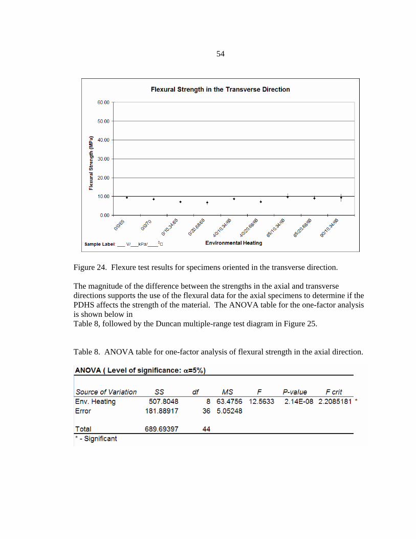
54

Figure 24. Flexure test results for specimens oriented in the transverse direction.

The magnitude of the difference between the strengths in the axial and transverse directions supports the use of the flexural data for the axial specimens to determine if the PDHS affects the strength of the material. The ANOVA table for the one-factor analysis is shown below in Table 8, followed by the Duncan multiple-range test diagram in Figure 25.

Table 8. ANOVA table for one-factor analysis of flexural strength in the axial direction.

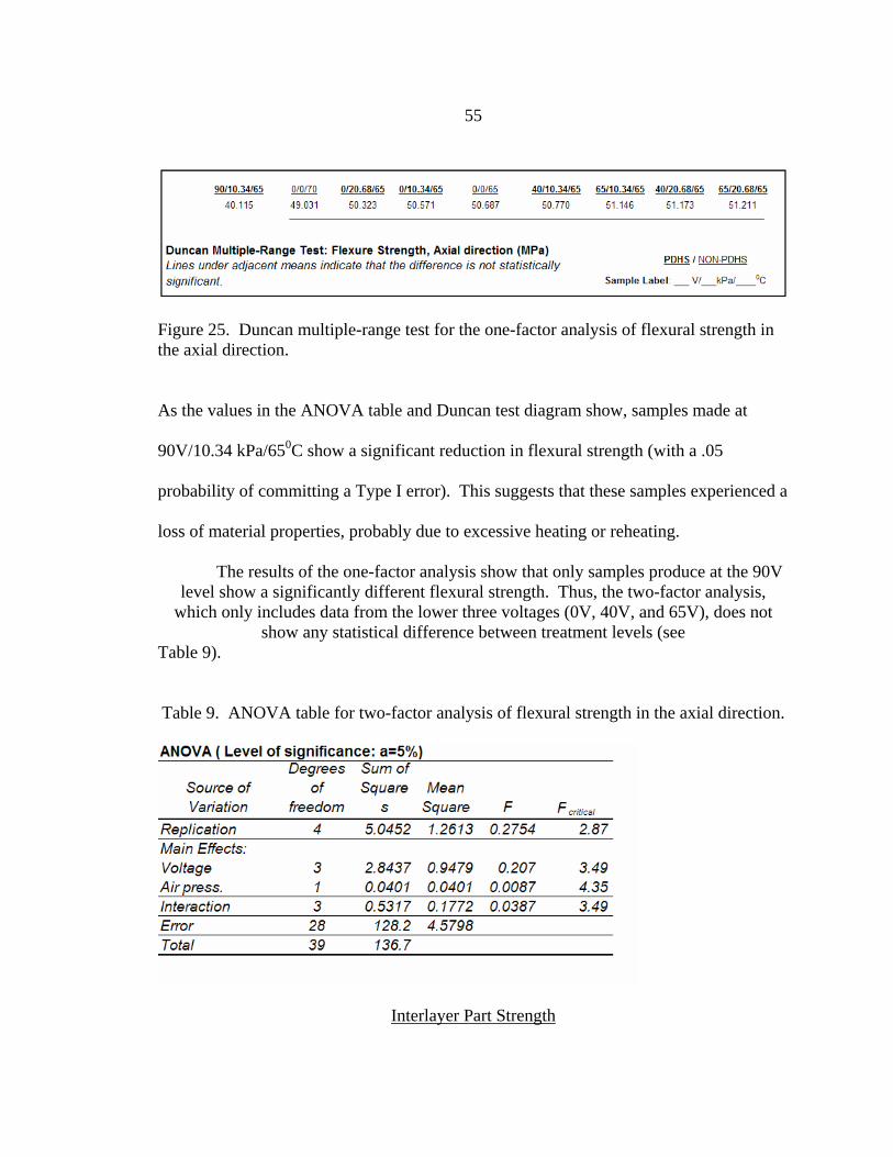
55

Figure 25. Duncan multiple-range test for the one-factor analysis of flexural strength in the axial direction.

As the values in the ANOVA table and Duncan test diagram show, samples made at

90V/10.34 kPa/650C show a significant reduction in flexural strength (with a .05

probability of committing a Type I error). This suggests that these samples experienced a

loss of material properties, probably due to excessive heating or reheating.

The results of the one-factor analysis show that only samples produce at the 90V level show a significantly different flexural strength. Thus, the two-factor analysis,

which only includes data from the lower three voltages (0V, 40V, and 65V), does not show any statistical difference between treatment levels (see

Table 9).

Table 9. ANOVA table for two-factor analysis of flexural strength in the axial direction.

Interlayer Part Strength

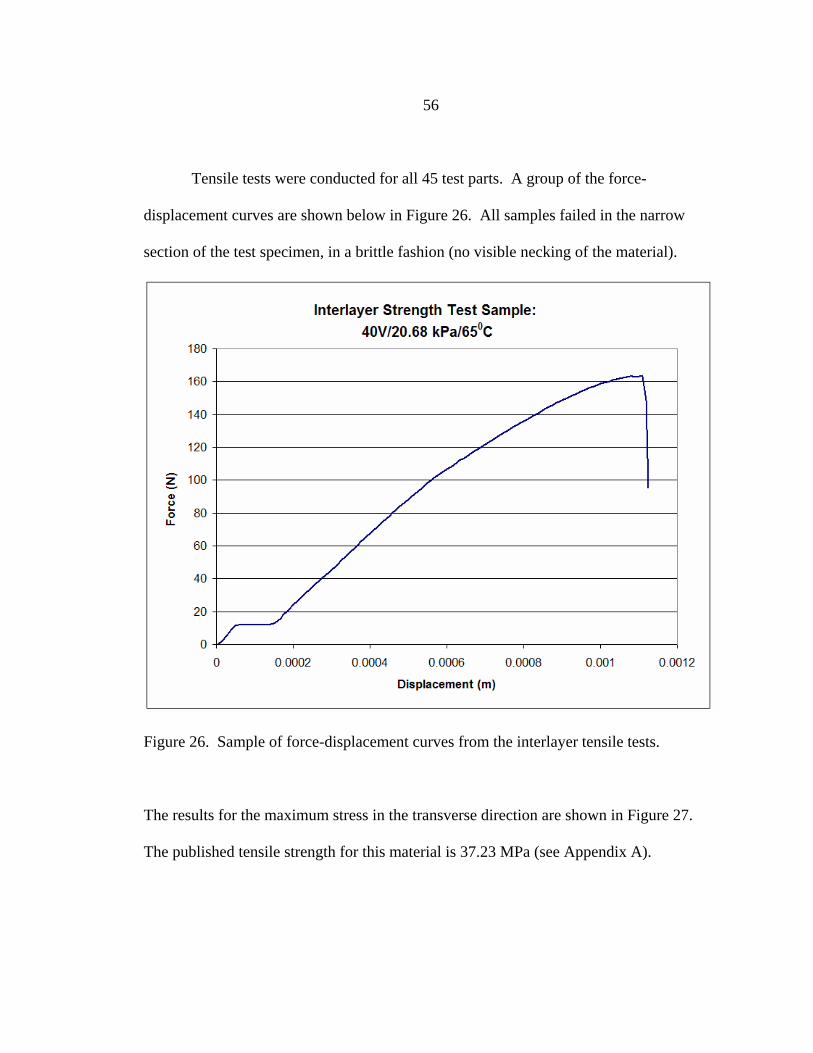
56

Tensile tests were conducted for all 45 test parts. A group of the force-

displacement curves are shown below in Figure 26. All samples failed in the narrow

section of the test specimen, in a brittle fashion (no visible necking of the material).

Figure 26. Sample of force-displacement curves from the interlayer tensile tests.

The results for the maximum stress in the transverse direction are shown in Figure 27.

The published tensile strength for this material is 37.23 MPa (see Appendix A).

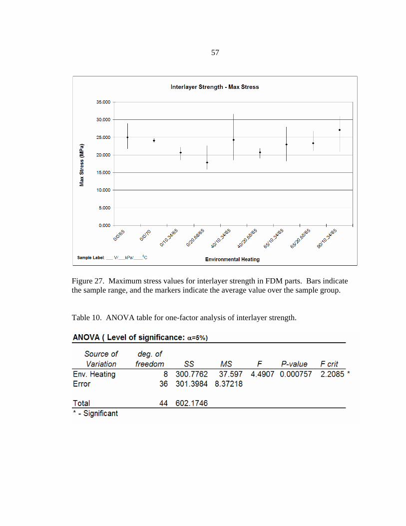
57

Figure 27. Maximum stress values for interlayer strength in FDM parts. Bars indicate the sample range, and the markers indicate the average value over the sample group.

Table 10. ANOVA table for one-factor analysis of interlayer strength.

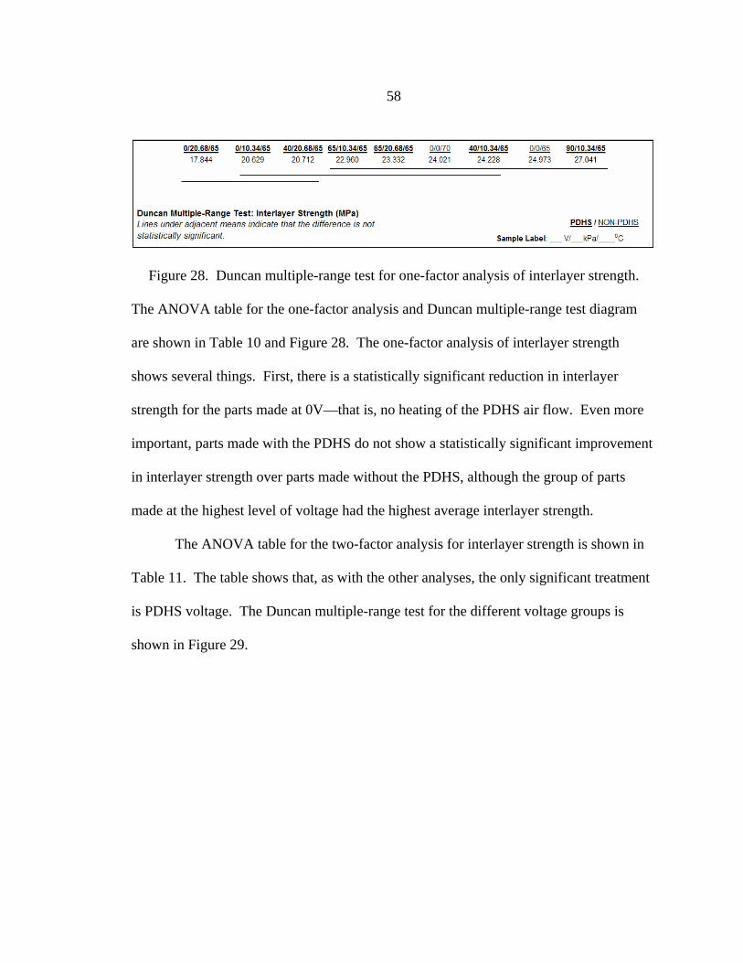
58

Figure 28. Duncan multiple-range test for one-factor analysis of interlayer strength.

The ANOVA table for the one-factor analysis and Duncan multiple-range test diagram

are shown in Table 10 and Figure 28. The one-factor analysis of interlayer strength

shows several things. First, there is a statistically significant reduction in interlayer

strength for the parts made at 0V—that is, no heating of the PDHS air flow. Even more

important, parts made with the PDHS do not show a statistically significant improvement

in interlayer strength over parts made without the PDHS, although the group of parts

made at the highest level of voltage had the highest average interlayer strength.

The ANOVA table for the two-factor analysis for interlayer strength is shown in

Table 11. The table shows that, as with the other analyses, the only significant treatment

is PDHS voltage. The Duncan multiple-range test for the different voltage groups is

shown in Figure 29.

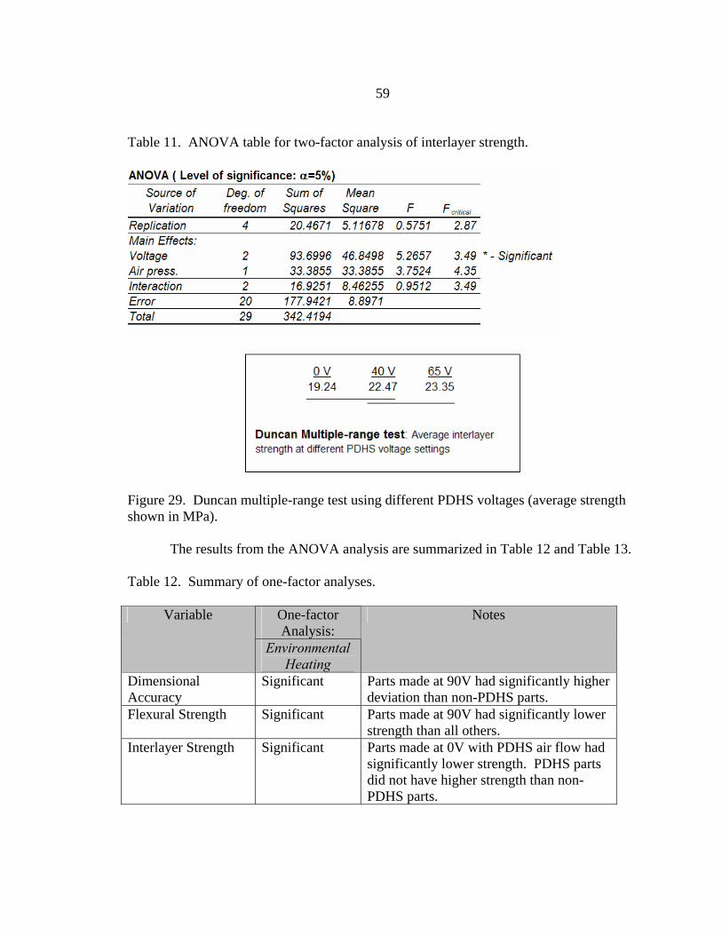
59

Table 11. ANOVA table for two-factor analysis of interlayer strength.

Figure 29. Duncan multiple-range test using different PDHS voltages (average strength shown in MPa).

The results from the ANOVA analysis are summarized in Table 12 and Table 13.

Table 12. Summary of one-factor analyses.

One-factor Analysis:

Variable

Environmental Heating

Notes

Dimensional Accuracy

Significant Parts made at 90V had significantly higher deviation than non-PDHS parts.

Flexural Strength Significant Parts made at 90V had significantly lower strength than all others.

Interlayer Strength Significant Parts made at 0V with PDHS air flow had significantly lower strength. PDHS parts did not have higher strength than non-PDHS parts.

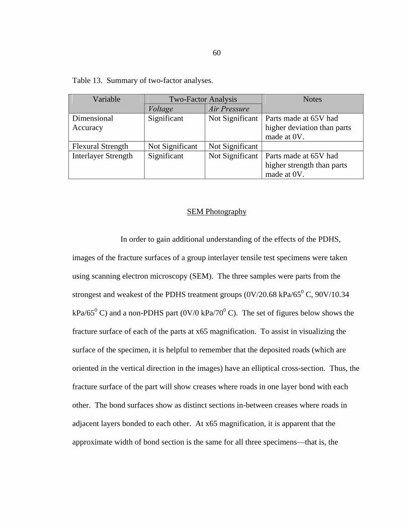
60

Table 13. Summary of two-factor analyses.

Two-Factor Analysis Variable Voltage Air Pressure

Notes

Dimensional Accuracy

Significant Not Significant Parts made at 65V had higher deviation than parts made at 0V.

Flexural Strength Not Significant Not Significant Interlayer Strength Significant Not Significant Parts made at 65V had

higher strength than parts made at 0V.

SEM Photography

In order to gain additional understanding of the effects of the PDHS,

images of the fracture surfaces of a group interlayer tensile test specimens were taken

using scanning electron microscopy (SEM). The three samples were parts from the

strongest and weakest of the PDHS treatment groups (0V/20.68 kPa/650 C, 90V/10.34

kPa/650 C) and a non-PDHS part (0V/0 kPa/700 C). The set of figures below shows the

fracture surface of each of the parts at x65 magnification. To assist in visualizing the

surface of the specimen, it is helpful to remember that the deposited roads (which are

oriented in the vertical direction in the images) have an elliptical cross-section. Thus, the

fracture surface of the part will show creases where roads in one layer bond with each

other. The bond surfaces show as distinct sections in-between creases where roads in

adjacent layers bonded to each other. At x65 magnification, it is apparent that the

approximate width of bond section is the same for all three specimens—that is, the

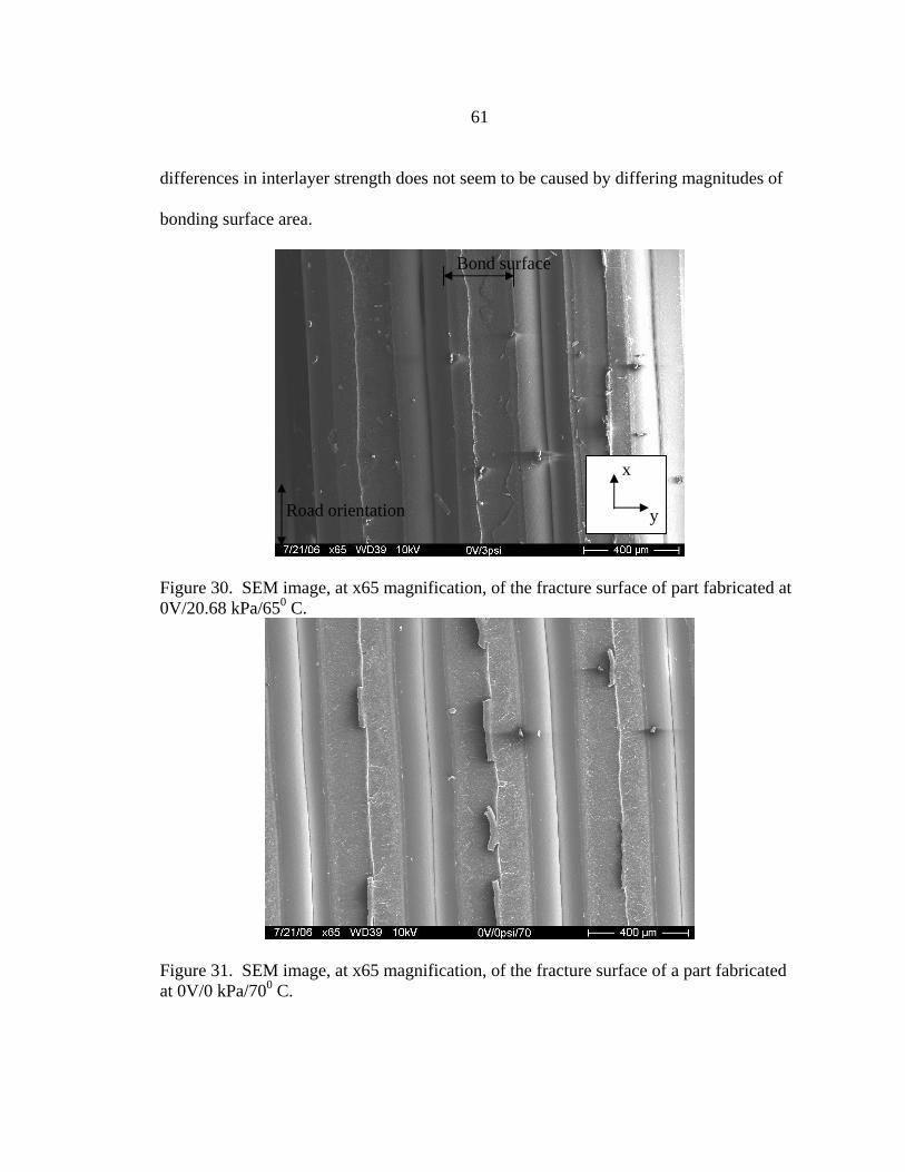
61

differences in interlayer strength does not seem to be caused by differing magnitudes of

bonding surface area.

Figure 30. SEM image, at x65 magnification, of the fracture surface of part fabricated at 0V/20.68 kPa/650 C.

Figure 31. SEM image, at x65 magnification, of the fracture surface of a part fabricated at 0V/0 kPa/700 C.

Bond surface

Road orientation

x

y

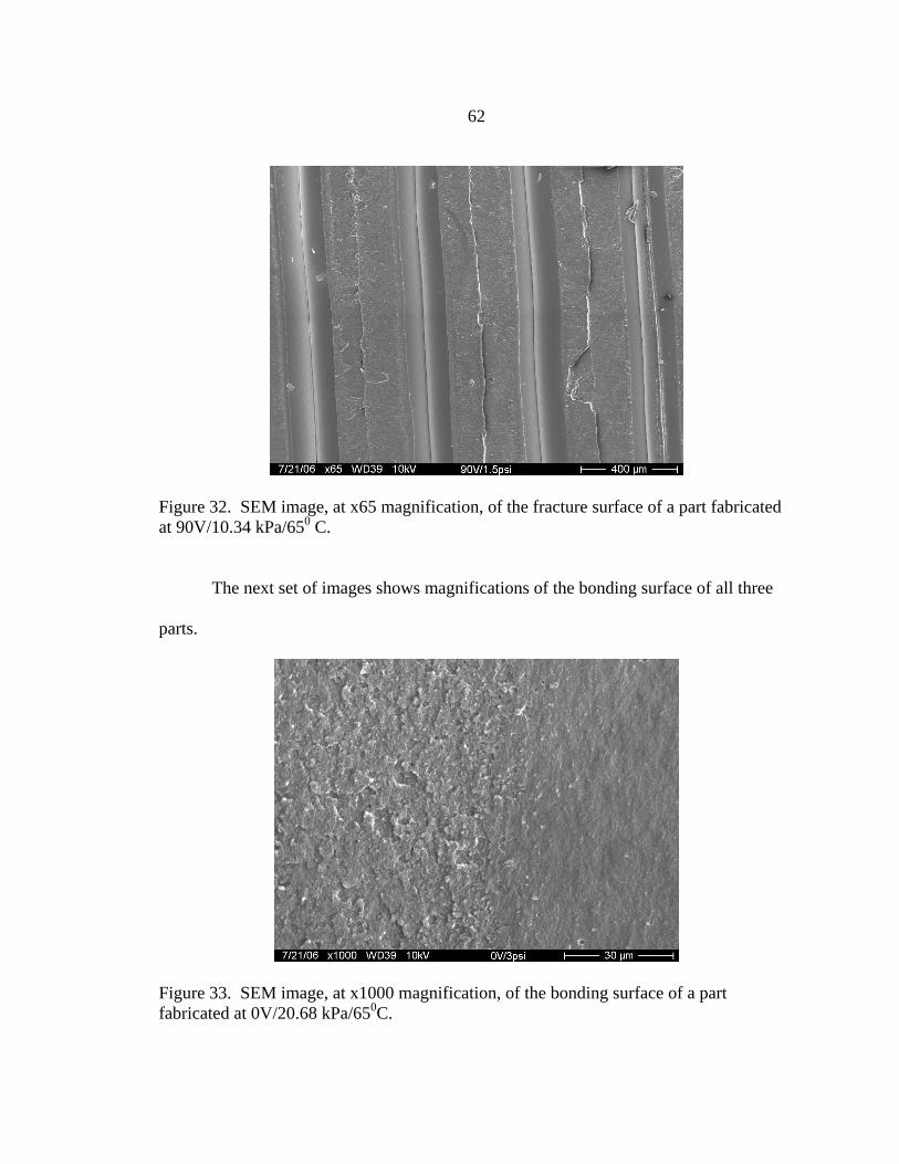
62

Figure 32. SEM image, at x65 magnification, of the fracture surface of a part fabricated at 90V/10.34 kPa/650 C.

The next set of images shows magnifications of the bonding surface of all three

parts.

Figure 33. SEM image, at x1000 magnification, of the bonding surface of a part fabricated at 0V/20.68 kPa/650C.

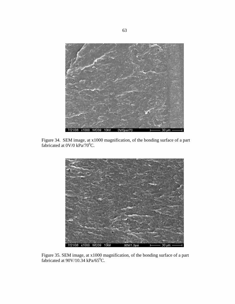
63

Figure 34. SEM image, at x1000 magnification, of the bonding surface of a part fabricated at 0V/0 kPa/700C.

Figure 35. SEM image, at x1000 magnification, of the bonding surface of a part fabricated at 90V/10.34 kPa/650C.

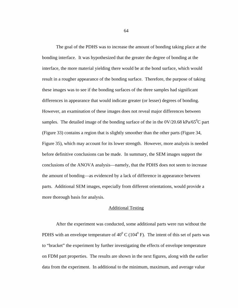
64

The goal of the PDHS was to increase the amount of bonding taking place at the

bonding interface. It was hypothesized that the greater the degree of bonding at the

interface, the more material yielding there would be at the bond surface, which would

result in a rougher appearance of the bonding surface. Therefore, the purpose of taking

these images was to see if the bonding surfaces of the three samples had significant

differences in appearance that would indicate greater (or lesser) degrees of bonding.

However, an examination of these images does not reveal major differences between

samples. The detailed image of the bonding surface of the in the 0V/20.68 kPa/650C part

(Figure 33) contains a region that is slightly smoother than the other parts (Figure 34,

Figure 35), which may account for its lower strength. However, more analysis is needed

before definitive conclusions can be made. In summary, the SEM images support the

conclusions of the ANOVA analysis—namely, that the PDHS does not seem to increase

the amount of bonding—as evidenced by a lack of difference in appearance between

parts. Additional SEM images, especially from different orientations, would provide a

more thorough basis for analysis.

Additional Testing After the experiment was conducted, some additional parts were run without the

PDHS with an envelope temperature of 400 C (1040 F). The intent of this set of parts was

to “bracket” the experiment by further investigating the effects of envelope temperature

on FDM part properties. The results are shown in the next figures, along with the earlier

data from the experiment. In additional to the minimum, maximum, and average value

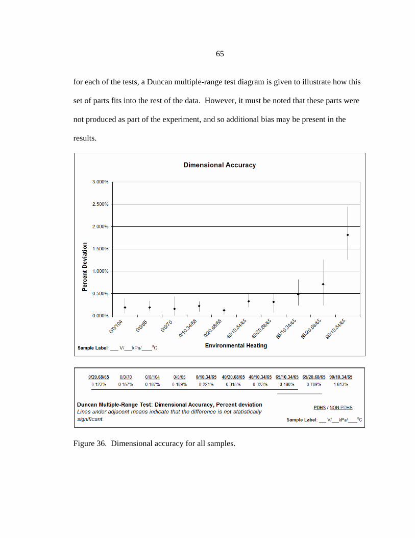
65

for each of the tests, a Duncan multiple-range test diagram is given to illustrate how this

set of parts fits into the rest of the data. However, it must be noted that these parts were

not produced as part of the experiment, and so additional bias may be present in the

results.

Figure 36. Dimensional accuracy for all samples.

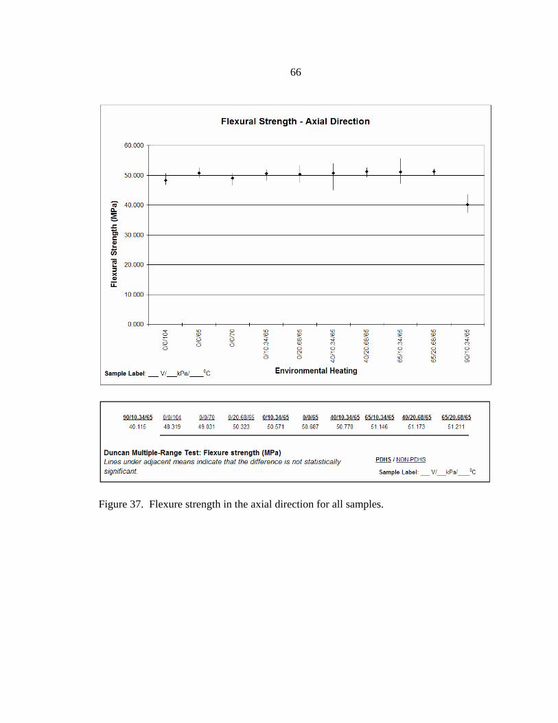
66

Figure 37. Flexure strength in the axial direction for all samples.

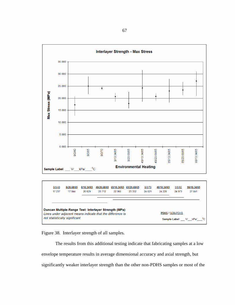
67

Figure 38. Interlayer strength of all samples.

The results from this additional testing indicate that fabricating samples at a low

envelope temperature results in average dimensional accuracy and axial strength, but

significantly weaker interlayer strength than the other non-PDHS samples or most of the

68

PDHS samples. These results are in agreement with the studies done by Yan et al and

Rodriguez et al discussed at length in the introduction [30,34].

69

CONCLUSIONS, RECOMMENDATIONS, AND FUTURE WORK The goal of this work was to investigate the potential for increasing FDM part

strength in the transverse direction through the development and implementation of a pre-

deposition heating system (PDHS). This system was built around a PVC welder designed

to weld thermoplastic materials using forced air, and used a two-nozzle design to apply

the heated air to the substrate material along the x-axis of the fabrication envelope. A

statistical experiment was designed to test the effects of this system in three variables:

interlayer part strength, dimensional accuracy, and axial flexural strength. A set of

samples was fabricated and tested for each of these variables, and the data was analyzed

using analysis of variance (ANOVA) techniques. Based on the results of the analysis and

observations made during PDHS development, several conclusions can be drawn.

Conclusions

Based on the ANOVA analysis, the PDHS did not result in significantly stronger

samples, and still showed presence of extreme anisotropy (as shown in the flexure tests).

The samples that displayed the strongest interlayer strength were PDHS samples

fabricated at the highest air temperature and lowest air flow, but these samples had the

worst dimensional accuracy and significantly weaker axial flexural strength. The

weakest parts were made when the envelope temperature was at its lowest setting (parts

fabricated at 0V/0 kPa/400C) or when there was a large amount of unheated air flow in

the envelope (parts fabricated at 0V/20.68 kPa/650C), which agrees with the findings of

70

Yan et al, who found that a large degree of air flow in the envelope significantly

degraded interlayer strength [34].

Clearly, the results indicate that the PDHS did not have the intended

improvements on FDM performance. However, based on observations made during the

development of the PDHS, the central issue appears to be the use of forced air as the

mechanism for heating the substrate—and the limitations of the PVC welder used to heat

the air—rather than the concept itself. The specifications of the PDHS were that a “no-

contact” heating source was necessary to keep from disrupting material deposition. At

that point in the development, it was thought that the force of the air flow would not be

sufficient to cause any disturbance in material deposition. However, when the air flow

was applied to the substrate just in front of the nozzle, it disrupted the deposition of

material, preventing the fabrication of good parts. The logical solution to this problem

would be to decrease the air flow and increase the temperature in order to maintain the

same amount of heat transfer to the substrate. This was attempted as far as the PVC

welder would allow, but even at the lowest air flow (the setting used in the experiment)

fabrication of good parts was impossible. Therefore, in order to make parts that were

geometrically accurate, the air flow had to be moved away from the optimal point of

application.

Another issue with the current design of the PDHS is the lack of precision in the

heating. The goal of the PDHS design was to keep the heating as localized as possible to

maintain the dimensional integrity of the part. However, the samples fabricated at the

highest temperature showed a reduction in both dimensional accuracy and material

71

properties. The SEM images showed that the mesostructure of these parts was virtually

identical to the non-PDHS parts, which seems to indicate that the dimensional

inaccuracies resulted from aberrations on a larger scale. The area over which the heated

air was applied was wide enough that each road was re-heated several times during

deposition. When the air temperature was hot enough (as during fabrication of parts

made at 90V), the roads were heated to the point of being softened—and thus more

susceptible to disturbance from the air flows on either side of the deposition head. If the

heating were more confined to the area of the substrate immediately preceding

deposition, this disturbance and excess re-heating of the roads would be limited, and the

dimensional integrity of the part could be maintained.

It is the opinion of the author that the concept underlying the design of the PDHS

is sound, and that some form of PDHS will be necessary to improve transverse strength to

the point where rapid manufacturing with FDM is feasible. The reason for this is that it is

impossible to raise the envelope temperature to the point where interlayer and inter-road

bonding is maximized without compromising the geometric integrity of the part.

Therefore, in order for this maximum bond strength to occur, some form of localized

heating must be present. Both of the shortcomings of the current system discussed in the

previous two paragraphs were identified prior to selection of the hardware, but it was

unknown at the time how significant these factors would be. This study is useful in

demonstrating how sensitive the FDM technology is to air flows around the point of

deposition, and establishes further design considerations for additional iterations of a pre-

deposition heating system. These considerations will be discussed in the next section.

72

In addition to the lessons learned regarding the PDHS, the assessment hierarchy

developed to test the effects of the PDHS is a useful product of this work. This analysis

methodology is not specific to this design, and so would fit any process change aimed at

increasing part strength in the transverse directions. The strengths of this analysis are

that it examines several part performance variables (interlayer strength, flexural strength,

and dimensional accuracy), so that transverse strength is not improved to the detriment of

dimensional accuracy and material strength. In addition, the use of ANOVA analysis

allows for changes in any of these variables to be examined for actual statistical

significance, which lessens the risk of making conclusions that are not supported by the

data. The hierarchy is summarized in more general terms in Figure 39.

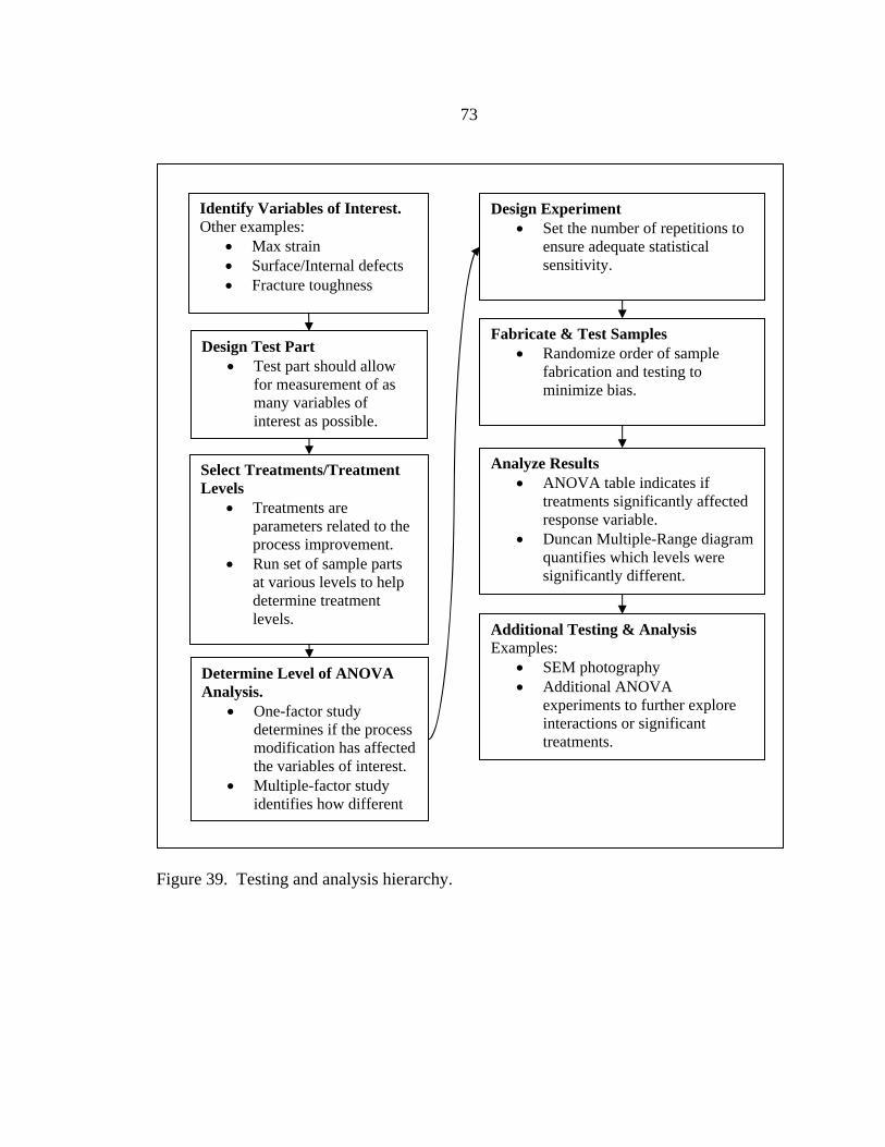
73

Figure 39. Testing and analysis hierarchy.

Design Test Part • Test part should allow

for measurement of as many variables of interest as possible.

Design Experiment • Set the number of repetitions to

ensure adequate statistical sensitivity.

Fabricate & Test Samples • Randomize order of sample

fabrication and testing to minimize bias.

Analyze Results • ANOVA table indicates if

treatments significantly affected response variable.

• Duncan Multiple-Range diagram quantifies which levels were significantly different.

Additional Testing & Analysis Examples:

• SEM photography • Additional ANOVA

experiments to further explore interactions or significant treatments.

Identify Variables of Interest. Other examples:

• Max strain • Surface/Internal defects • Fracture toughness

Select Treatments/Treatment Levels

• Treatments are parameters related to the process improvement.

• Run set of sample parts at various levels to help determine treatment levels.

Determine Level of ANOVA Analysis.

• One-factor study determines if the process modification has affected the variables of interest.

• Multiple-factor study identifies how different

74

Recommendations and Future Work Future work in this area will involve improving the design of the PDHS. Based

on the results discussed in the previous section, several recommendations can be made

with regard to future iterations of a pre-deposition heating system.

• Given the sensitivity of FDM to air flow, other heating technologies may be more

appropriate than forced air. These may include other “no-contact” solutions, such

as the other options listed in this work (or others that the author did not consider).

Also, there may be some minimal-contact solutions (e.g. where contact is made

with the substrate without significantly disturbing the material) that may be

effective in this application.

• Additional work could be done to model and characterize the actual temperature

of the substrate material at different points during deposition (prior to heating by

the PDHS, after heating by the PDHS but prior to deposition, and after

deposition), if further iterations of PDHS are warranted. This could include

lumped parameter models or finite element models and would help set the

requirements of the PDHS heating system (e.g. heat flux required to achieve the

critical substrate temperature).

• In addition to modeling the process, future work should also include a study to

help determine what the critical temperature of the substrate should be for to

ensure bonding via molecular diffusion. As discussed in the literature review,

there was some disagreement in the literature as to which material property

75

corresponded to the critical bonding temperature (Vicat softening temperature vs.

glass transition temperature), and additional analysis should be done to resolve

this question. A possible method of establishing this would be to heat treat of a

set of FDM parts at different temperatures and use SEM microscopy to observe

changes in the macrostructure that might indicate greater levels of molecular

diffusion.

• Another recommendation would be to relax the constraint which prohibited

permanent modification to the FDM machine. Having the option to make

modifications to allow for easier integration between the PDHS and FDM

deposition head could greatly simplify the hardware design and implementation of

the PDHS.

• As discussed in the previous section, the assessment hierarchy developed in the

work could be applied to any process improvement (e.g. PDHS design using

microwave, process parameter changes, etc.) aimed at increasing transverse part

strength without adversely affecting dimensional accuracy or material strength.

Design is an iterative process, and it is the author’s hope that this work will be useful in

the design of the next PDHS so that the potential of FDM in rapid manufacturing will be

fulfilled.

76

REFERENCES CITED 1. Wohlers, T.T., Wohler’s Report 2003: Rapid Prototyping, Tooling &

Manufacturing State of the Industry, Annual Worldwide Progress Report, Wohlers Associates, Inc., Fort Collins, CO., p. 13. (2003)

2. Mcmains, S., “Layered Manufacturing Technologies”, Communications of the

ACM, Vol. 48 No. 6, p.52. (2005)

3. Bellini, A., and Guçeri, S., “Mechanical characterization of parts fabricated using fused deposition modeling”, Rapid Prototyping Journal, Vol. 9 No. 4, pp. 252-264. (2003)

4. [3], p. 262.

5. [2], p. 53.

6. [1], p. 113.

7. Stratasys, Inc (ed.). “Fast Build options”. QuickSlice v. 5.0 Help Guide. (1997)

8. Stratasys, Inc (ed.) “Slicing an STL file”, QuickSlice v. 5.0 Help Guide. (1997)

9. [2], p. 52.

10. [2], p. 53.

11. [1], p. 265.

12. Bellini, A., Shor, L. and Guçeri, S., “New developments in fused deposition

modeling of ceramics”, Rapid Prototyping Journal, Vol. 11 No.4, pp. 214-220. (2005)

13. Masood, S.H., and Song, W.Q., “Development of new metal/polymer materials

for rapid tooling using Fused deposition modelling”, Materials and Design, No. 25, pp.587-594. (2004)

14. Yan, Y., Rendong, W., et. al., “Biomaterial forming research using RP

technology”, Rapid Prototyping Journal, Vol. 9 No. 3, pp.142-149. (2003)

15. Grimm, T., “Fused Deposition Modelling: A Technology Evaluation”, Time Compression Technologies, Vol. 2 No. 2, pp. 1-6. (2003)

16. [15], p.5.

77

17. Agarwala, M., Jamalabad, V., et. al., “Structural quality of parts processed by

fused deposition”, Rapid Prototyping Journal, Vol. 2 No. 4, pp. 4-19. (1996)

18. Han, W., Jafari, M.A., Danforth, S.C. and Safari, “Tool path-based deposition planning in fused deposition processes”, Transactions of The ASME Journal of Manufacturing Science and Engineering, Vol. 124, pp. 462-72. (2002)

19. Han, W., Jafari, M., and Seyed, K. (2003), “Process speeding up via deposition

planning in fused deposition-based layered manufacturing processes”, Rapid Prototyping Journal, Vol. 9 No. 4, pp. 212-218.

20. Langrana, N., Qiu, D., et. al., “Virtual simulation and video microscopy for fused

deposition methods”, Material and Design, No. 21, pp.75-82. (2000)

21. Anitha, R., Arunachalam, S., Radhakrishnan, P., (2001), “Critical parameters influencing the quality of prototypes in fused deposition modelling” Journal of Materials Processing Technology. Vol 118, pp. 385-388. (2001)

22. Bose, S., Darsell, J., et. al. (2002), “Pore size and pore volume effects on alumina

and TCP ceramic scaffolds”, Material Science and Engineering, C 23, pp. 479-486. (2002)

23. Darsell, J., Susmita, B., et. al., “From CT Scan to Ceramic Bone Graft”, Journal

of American Ceramic Society, Vol. 86 No. 7, pp. 1076-80. (2003)

24. Shofner, M.L., Lozano, K., Rodriguez-Macias, F.J., and Barrera, E.V., “Nanofiber-Reinforced Polymers Prepared by Fused Deposition Modeling”, Journal of Applied Polymer Science, Vol. 89, pp.3081-3090. (2002)

25. Wu, G., Langrana, N.A., Sadanji, R., and Danforth, S., “Solid freeform

frabrication of metal components using fused deposition of metals”, Materials and Design, Vol. 23, pp.97-105. (2002)

26. Yan, Y., Rendong, W., et. al., “Biomaterial forming research using RP

technology”, Rapid Prototyping Journal, Vol. 9 No. 3, pp.142-149. (2003) 27. Bellini, A., and Guçeri, S., “Mechanical characterization of parts fabricated using

fused deposition modeling”, Rapid Prototyping Journal, Vol. 9 No. 4, pp. 252-264. (2003)

78

28. Rodriguez, J.F., Thomas, J.P. and Renaud, J.E., “Characterizing the microstructure of fused deposition polymer components”, CAE and Intelligent Processing of Polymeric Materials, MD-Vol. 79, ASME, NY, pp.299-308. (1997)

29. Rodriguez, J.F., Thomas, J.P., and Renaud, J.E., “Characterization of the

mesostructure of fused-deposition acrylonitrile-butadience-styrene materials”, Rapid Prototyping Journal, Vol. 6 No. 3, pp.175-185. (2000)

30. Rodriguez, J.F., Thomas, J.P. and Renaud, J.E., “Tailoring the mechanical

properties of fused-deposition manufactured components”, Proc. Rapid Prototyping and Manufacturing ’99, Vol. 3, Society of Manufacturing Engineers, Dearborn, MI, pp.629-43. (1999)

31. Rodriguez, J.F., Thomas, J.P. and Renaud, J.E., “Mechanical behavior of

acrylonitrile butadience styrene fused deposition materials modeling”, Rapid Prototyping Journal, Vol. 9 No. 4, pp.219-230. (2003)

32. Rodriguez, J.F., Thomas, J.P. and Renaud, J.E., “Design of Fused-Deposition

ABS Components for Stiffness and Strength”, Journal of Mechanical Design, Vol. 125, pp.545-551. (2003)

33. Kulkarni, P., and Dutta, D. (1999), “Deposition Strategies and Resulting Part

Stiffnesses in Fused Deposition Modeling”, ASME Journal of Manufacturing Science and Engineering, Vol. 121, pp. 93-101.

34. Yan, Y., Zhang, R., Guodong, H., and Yuan, X., “Research on the bonding of

material paths in melted extrusion modeling”, Materials and Design, Vol. 21, pp. 93-99. (2000)

35. Rodriguez, J.F., Thomas, J.P. and Renaud, J.E., “Tailoring the mechanical

properties of fused-deposition manufactured components”, Proc. Rapid Prototyping and Manufacturing ’99, Vol. 3, Society of Manufacturing Engineers, Dearborn, MI, p. 630 (1999)

36. Yan, Y., Zhang, R., Guodong, H., and Yuan, X., “Research on the bonding of

material paths in melted extrusion modeling”, Materials and Design, Vol. 21, pp. 93-99. (2000)

37. [21], p.631 38. [25], p.95 39. Automation Creations (ed.), Matweb (2006)

79

<http://www.matweb.com/search/SpecificMaterial.asp?bassnum=O1105>

40. Yardimci, M.A. and Güceri, S., “Conceptual framework for the thermal process modelling of fused deposition” Rapid Prototyping Journal, Vol. 2 No. 2, pp. 26-31. (1996)

41. Bird, R.B., Stewart, W.E., and Lightfoot, E.N., Transport Phenomena 2nd ed.

New York: John Wiley & Sons, Inc. (2002) 42. [21], p.642 43. TWI Ltd (ed.), “TWI Knowledge Summary: Laser welding of plastics”, TWI

World Centre for Materials Joining Technology. (2006) Retrieved June 14, 2006, from

<http://www.twi.co.uk/j32k/protected/band_3/ksab002.html>

44. Froment, Ian. “Ultrasonic welding of thermoplastics - a guide to best practice”, TWI World Centre for Materials Joining Technology. (2006) Retrieved June 16, 2006 from

<http://www.twi.co.uk/j32k/protected/band_8/bpuwts01.html>

45. Cundy, V. Personal communication. May 11, 2006. 46. ASTM D638-02a, “Standard Test Method for Tensile Properties of Plastics”,

American Society for Testing and Materials, Conshohocken, PA. (2003) 47. Freund, John E. and Miller, Irwin. Miller and Freund’s Probability and Statistics

for Engineers. Richard A. Johnson -6th ed. Upper Saddle River, NJ: Prentice-Hall, Inc. p. 396. (2000)

48. Schillings, P. Lecture notes. October 16, 2001.

49. [36], p. 395.

50. Munson, B.R., Young, D.F, and Okiishi, T.H. Fundamentals of Fluid Mechanics.

4th ed. John Wiley & Sons, Inc. p.832. (2002)

51. ASTM D790, “Standard Test Method for Flexure Properties of Plastsics”, American Society for Testing and Materials, Conshohocken, PA. (2003)

80

APPENDICES

81

APPENDIX A

EQUIPMENT, MATERIAL INFORMATION

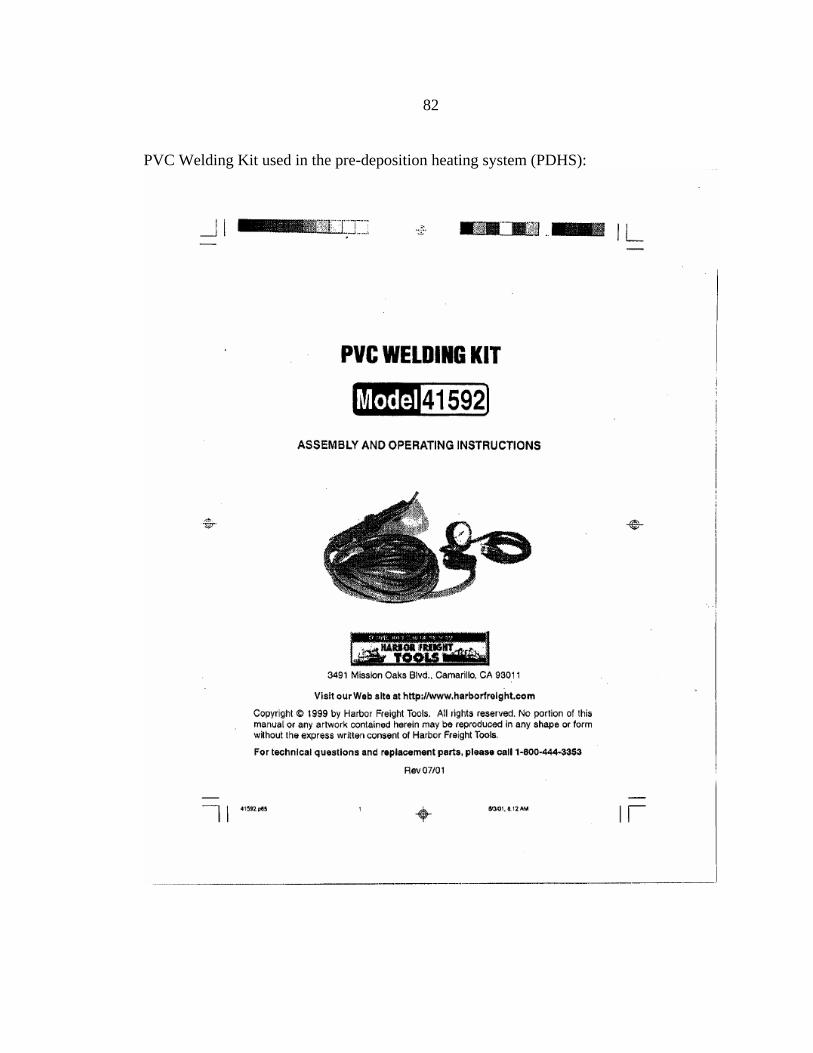
82

PVC Welding Kit used in the pre-deposition heating system (PDHS):

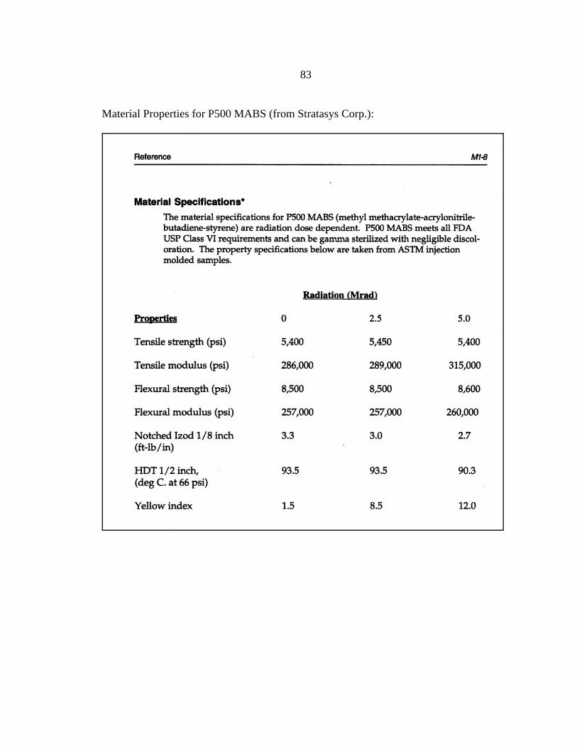
83

Material Properties for P500 MABS (from Stratasys Corp.):

84

Recommended FDM Settings for P500 MABS (from Stratasys Corp.):

85

APPENDIX B

ANOVA CALCULATIONS

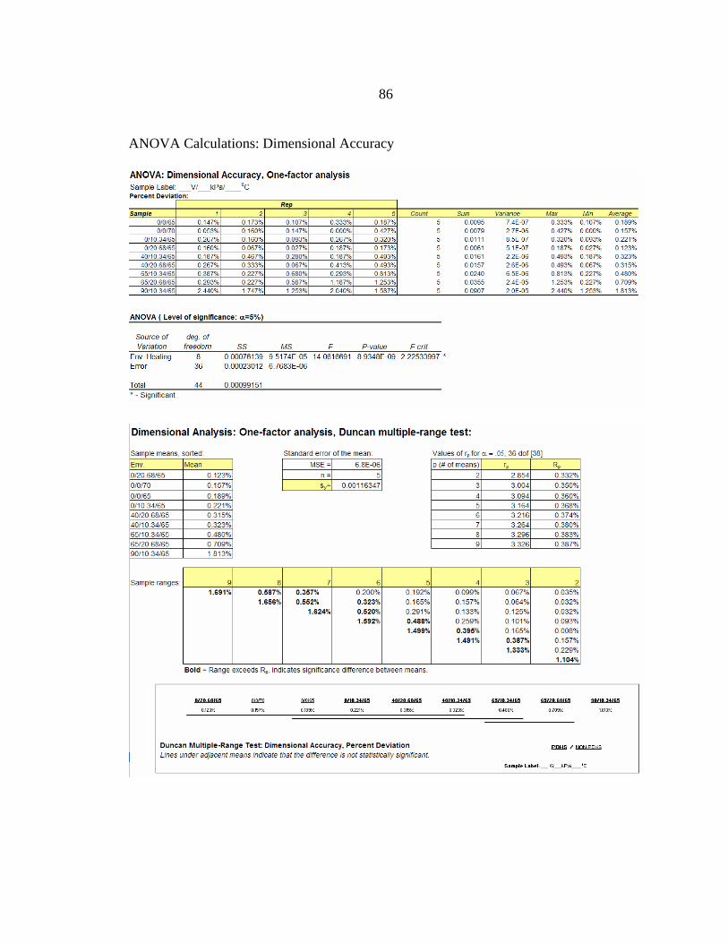
86

ANOVA Calculations: Dimensional Accuracy

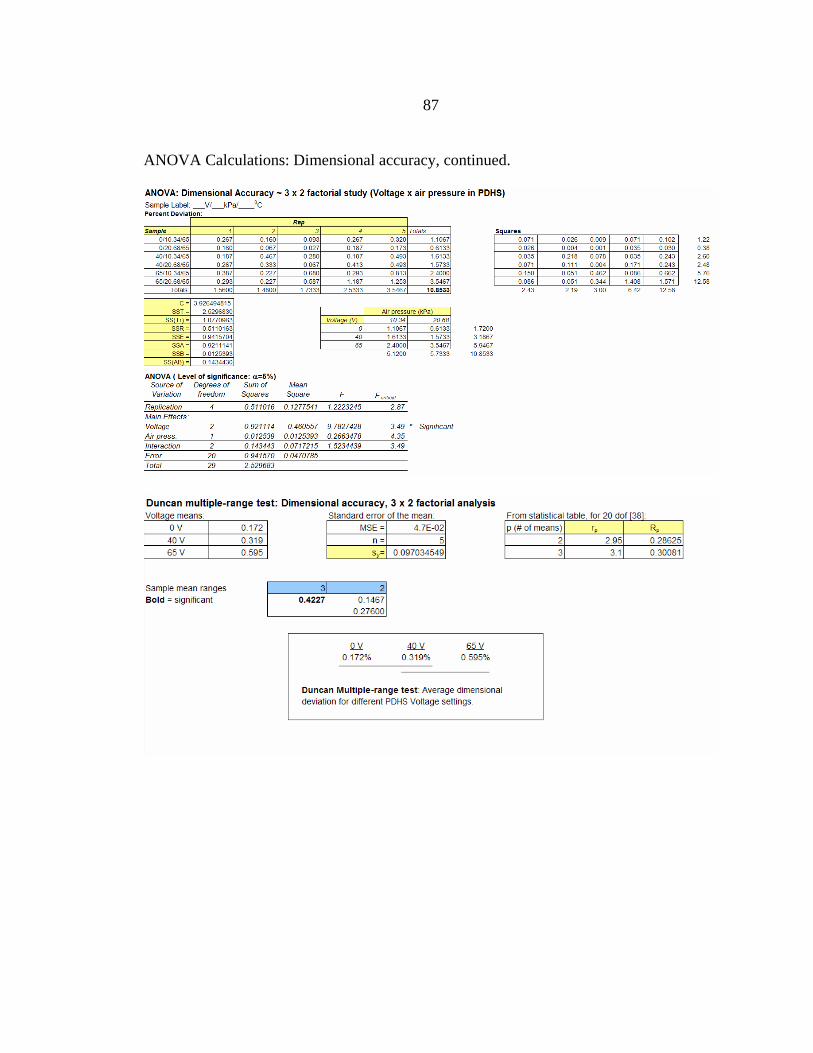
87

ANOVA Calculations: Dimensional accuracy, continued.

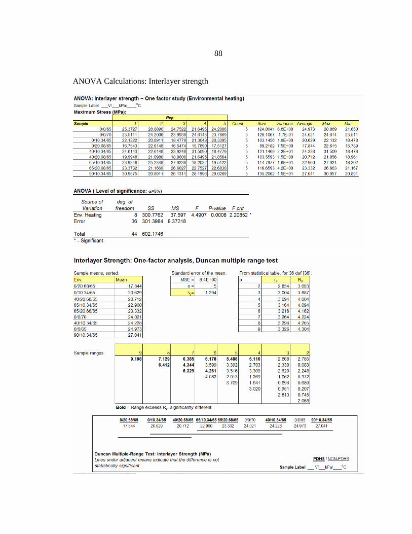
88

ANOVA Calculations: Interlayer strength

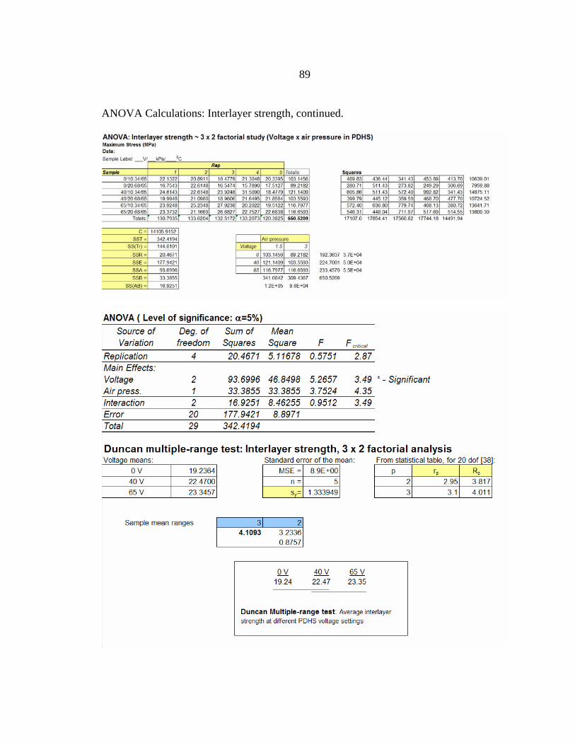
89

ANOVA Calculations: Interlayer strength, continued.

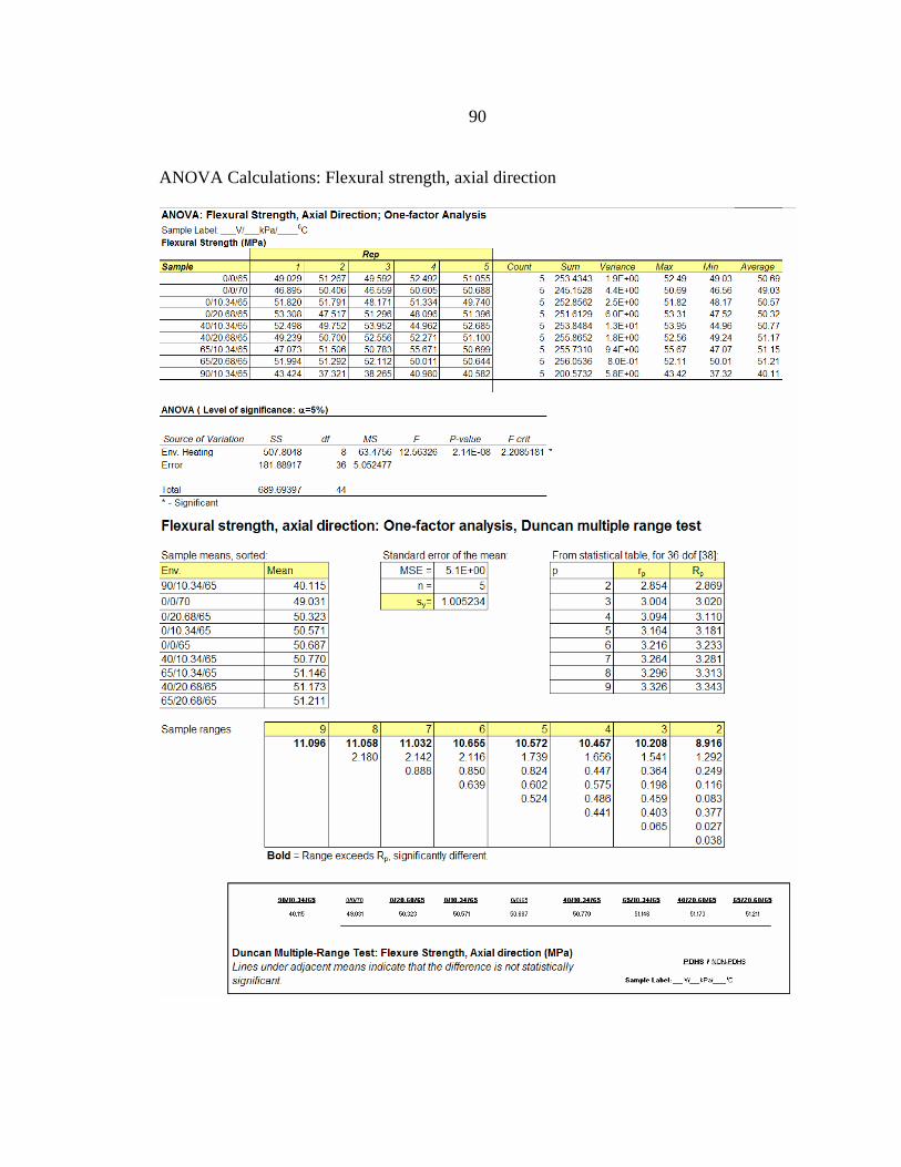
90

ANOVA Calculations: Flexural strength, axial direction

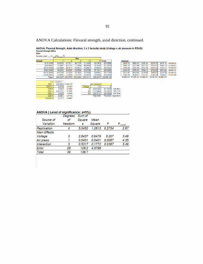
91

ANOVA Calculations: Flexural strength, axial direction, continued.

92

APPENDIX C

EXIT FLOW RATE CALCULATIONS

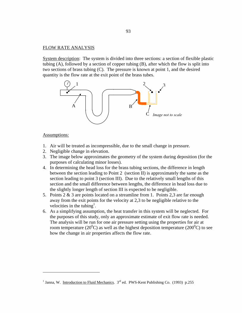
93

FLOW RATE ANALYSIS

System description: The system is divided into three sections: a section of flexible plastic tubing (A), followed by a section of copper tubing (B), after which the flow is split into two sections of brass tubing (C). The pressure is known at point 1, and the desired quantity is the flow rate at the exit point of the brass tubes.

Assumptions:

1. Air will be treated as incompressible, due to the small change in pressure. 2. Negligible change in elevation. 3. The image below approximates the geometry of the system during deposition (for the

purposes of calculating minor losses). 4. In determining the head loss for the brass tubing sections, the difference in length

between the section leading to Point 2 (section II) is approximately the same as the section leading to point 3 (section III). Due to the relatively small lengths of this section and the small difference between lengths, the difference in head loss due to the slightly longer length of section III is expected to be negligible.

5. Points 2 & 3 are points located on a streamline from 1. Points 2,3 are far enough away from the exit points for the velocity at 2,3 to be negligible relative to the velocities in the tubing1.

6. As a simplifying assumption, the heat transfer in this system will be neglected. For the purposes of this study, only an approximate estimate of exit flow rate is needed. The analysis will be run for one air pressure setting using the properties for air at room temperature (200C) as well as the highest deposition temperature (2000C) to see how the change in air properties affects the flow rate.

1 Janna, W. Introduction to Fluid Mechanics. 3rd ed. PWS-Kent Publishing Co. (1993) p.255

A BC

1 2 3

Image not to scale

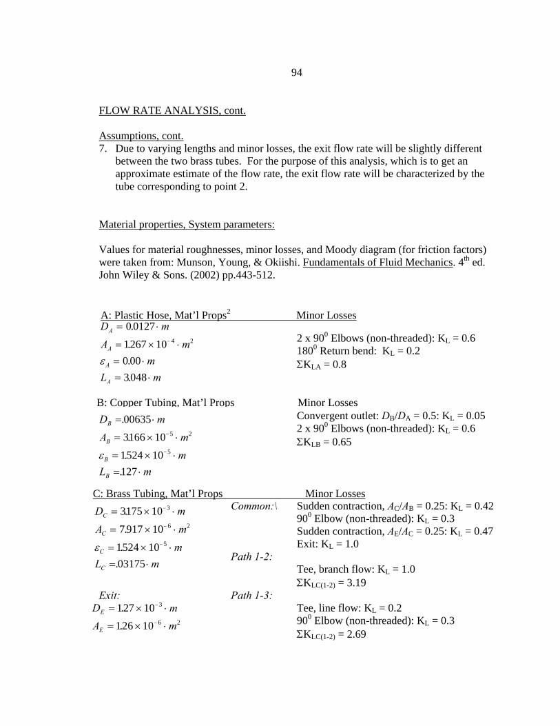
94

FLOW RATE ANALYSIS, cont.

Assumptions, cont. 7. Due to varying lengths and minor losses, the exit flow rate will be slightly different

between the two brass tubes. For the purpose of this analysis, which is to get an approximate estimate of the flow rate, the exit flow rate will be characterized by the tube corresponding to point 2.

Material properties, System parameters:

Values for material roughnesses, minor losses, and Moody diagram (for friction factors) were taken from: Munson, Young, & Okiishi. Fundamentals of Fluid Mechanics. 4th ed. John Wiley & Sons. (2002) pp.443-512.

2 x 900 Elbows (non-threaded): KL = 0.6 1800 Return bend: KL = 0.2 ΣKLA = 0.8

Convergent outlet: DB/DA = 0.5: KL = 0.05 2 x 900 Elbows (non-threaded): KL = 0.6 ΣKLB = 0.65

Common:\ Sudden contraction, AC/AB = 0.25: KL = 0.42

900 Elbow (non-threaded): KL = 0.3 Sudden contraction, AE/AC = 0.25: KL = 0.47 Exit: KL = 1.0 Path 1-2: Tee, branch flow: KL = 1.0

ΣKLC(1-2) = 3.19 Exit: Path 1-3: Tee, line flow: KL = 0.2

900 Elbow (non-threaded): KL = 0.3 ΣKLC(1-2) = 2.69

A: Plastic Hose, Mat’l Props2 Minor Losses D mA m

mL m

A

A

A

A

= ⋅

= × ⋅= ⋅= ⋅

−

0 01271267 100 003048

4 2

....

ε

D mA m

mL m

B

B

B

B

= ⋅

= × ⋅

= × ⋅= ⋅

−

−

..

..

006353166 10

1524 10127

5 2

5ε

B: Copper Tubing, Mat’l Props Minor Losses

C: Brass Tubing, Mat’l Props Minor Losses D mA m

mL m

C

C

C

C

= × ⋅

= × ⋅

= × ⋅= ⋅

−

−

−

3175 107 917 10

1524 1003175

3

6 2

5

.

..

.ε

D mA m

E

E

= × ⋅

= × ⋅

−

−

127 10126 10

3

6 2

..

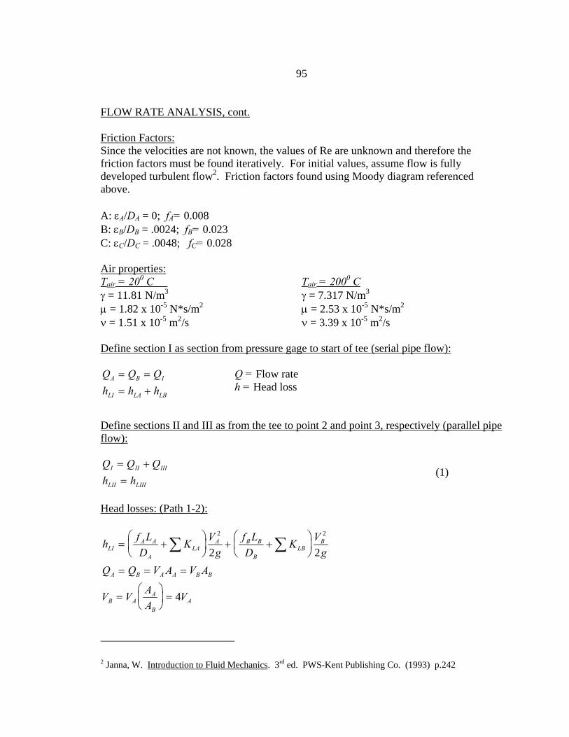
95

FLOW RATE ANALYSIS, cont.

Friction Factors: Since the velocities are not known, the values of Re are unknown and therefore the friction factors must be found iteratively. For initial values, assume flow is fully developed turbulent flow2. Friction factors found using Moody diagram referenced above. A: εA/DA = 0; fA= 0.008 B: εB/DB = .0024; fB= 0.023 C: εC/DC = .0048; fC= 0.028 Air properties: Tair = 200 C Tair = 2000 C γ = 11.81 N/m3 γ = 7.317 N/m3 μ = 1.82 x 10-5 N*s/m2 μ = 2.53 x 10-5 N*s/m2 ν = 1.51 x 10-5 m2/s ν = 3.39 x 10-5 m2/s Define section I as section from pressure gage to start of tee (serial pipe flow): Q = Flow rate h = Head loss Define sections II and III as from the tee to point 2 and point 3, respectively (parallel pipe flow): Q Q Qh h

I II III

LII LIII

= +=

(1)

Head losses: (Path 1-2):

h f LD

K Vg

f LD

K Vg

Q Q V A V A

V V AA

V

LIA A

ALA

A B B

BLB

B

A B A A B B

B AA

BA

= +⎛⎝⎜

⎞⎠⎟ + +

⎛⎝⎜

⎞⎠⎟

= = =

=⎛⎝⎜

⎞⎠⎟ =

∑ ∑2 2

2 2

4

2 Janna, W. Introduction to Fluid Mechanics. 3rd ed. PWS-Kent Publishing Co. (1993) p.242

Q Q Qh h h

A B I

LI LA LB

= == +

96

FLOW RATE ANALYSIS, cont. (2) (3) (4) Energy Equation for conduit flow between two points: (5) From the assumptions, system description: p1 = pressure gage; p2 = 0 V1 = VA; V2 = 0; z1-z2 = 0 (6) Substituting expressions (2), (3) into (6) and rearranging:

( ) ( )( )

( )

h f LD

K Vg

f LD

K Vg

h Vf f

g

h f LD

K Vg

Vf

g

LIA A

ALA

A B B

BLB

A

LI AA B

LIIC C

CLC

IIII

c

= +⎛⎝⎜

⎞⎠⎟ + +

⎛⎝⎜

⎞⎠⎟

=+ + +⎛

⎝⎜⎜

⎞

⎠⎟⎟

= +⎛⎝⎜

⎞⎠⎟ =

+⎛⎝⎜

⎞⎠⎟

∑ ∑

∑ −

2 2

2

2

22

216

2

240 0 8 16 20 0 652

210 3192

. .

.(1 )

p Vg

z p V z h hLI LII1 1

2

12 2

2

22γ γ γ+ + = + + + +

( )( ) ( )( )( )( )( )( )

h h

f LD

K Vg

f LD

K Vg

f V f V

Vf Vf

LII LIII

C CII

CLC

II C CIII

CLC

III

c II c III

IIIc II

c

=

+⎛⎝⎜

⎞⎠⎟ = +

⎛⎝⎜

⎞⎠⎟

+ = +

=+

+

− −∑ ∑(1 ) (1 )

. .

..

2

2

3

2

2 2

2

2 2

10 319 16 2 69

10 31916 2 69

( ) ( )( ) ( )p Vg

Vf f

gV

fg

II

A BII

c12

2 2

2240 0 8 16 20 0 65

210 3192γ

+ =+ + +⎛

⎝⎜⎜

⎞

⎠⎟⎟ +

+⎛

⎝⎜

⎞

⎠⎟

. . .

p Vg

h hILI LII

12

2γ+ = +

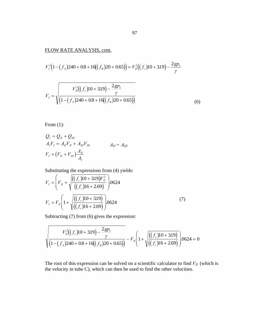
97

FLOW RATE ANALYSIS, cont. (6) From (1): Substituting the expressions from (4) yields: (7) Subtracting (7) from (6) gives the expression:

( )( )( ) ( )( )( )

( )( )( )( )

V f gp

f fV

ff

II c

A BII

c

c

2 110 319 2

1 240 0 8 16 20 0 651

10 31916 2 69

0624 0+ −

− + + +− +

+

+

⎛

⎝⎜⎜

⎞

⎠⎟⎟

=.

. .

.

..γ

The root of this expression can be solved on a scientific calculator to find VII (which is the velocity in tube C), which can then be used to find the other velocities.

( ) ( )( )( ) ( )( )V f f V f gpI A B II c2 2 11 240 0 8 16 20 0 65 10 319 2

− + + + = + −. . .γ

( )( )( ) ( )( )( )V

V f gp

f fI

II c

A B

=+ −

− + + +

2 110 319 2

1 240 0 8 16 20 0 65

.

. .γ

( )

Q Q QA V A V A V

V V V AA

I II III

I I II II III III

I II IIIII

I

= += +

= +

AII = AIII

( )( )( )( )

( )( )( )( )

V Vf Vf

V Vff

I IIc II

c

I IIc

c

= ++

+

⎛

⎝⎜⎜

⎞

⎠⎟⎟

= ++

+

⎛

⎝⎜⎜

⎞

⎠⎟⎟

10 31916 2 69

0624

110 31916 2 69

0624

2..

.

.

..

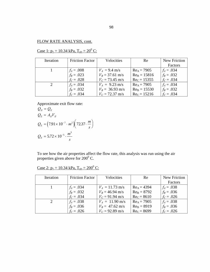
98

FLOW RATE ANALYSIS, cont. Case 1: p1 = 10.34 kPa, Tair = 200 C:

Iteration Friction Factor Velocities Re New Friction Factors

1 fA = .008 fB = .023 fC = .028

VA = 9.4 m/s VB = 37.61 m/s VC = 73.45 m/s

ReA = 7905 ReB = 15816 ReC = 15355

fA = .034 fB = .032 fC = .034

2 fA = .034 fB = .032 fC = .034

VA = 9.23 m/s VB = 36.93 m/s VC = 72.37 m/s

ReA = 7905 ReB = 15530 ReC = 15216

fA = .034 fB = .032 fC = .034

Approximate exit flow rate:

( )

Q QQ A V

Q m ms

Q ms

II E

E II II

E

E

==

= × ⋅ ⋅⎛⎝⎜

⎞⎠⎟

= × ⋅

−

−

7 91 10 72 37

5 72 10

7 2

53

. .

.

To see how the air properties affect the flow rate, this analysis was run using the air properties given above for 2000 C. Case 2: p1 = 10.34 kPa, Tair = 2000 C:

Iteration Friction Factor Velocities Re New Friction Factors

1 fA = .034 fB = .032 fC = .034

VA = 11.73 m/s VB = 46.94 m/s VC = 91.94 m/s

ReA = 4394 ReB = 8792 ReC = 8610

fA = .038 fB = .036 fC = .026

2 fA = .038 fB = .036 fC = .026

VA = 11.90 m/s VB = 47.62 m/s VC = 92.89 m/s

ReA = 7905 ReB = 8919 ReC = 8699

fA = .038 fB = .036 fC = .026

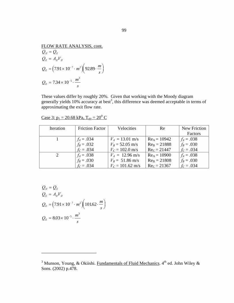
99

FLOW RATE ANALYSIS, cont.

( )

Q QQ A V

Q m ms

Q ms

II E

E II II

E

E

==

= × ⋅ ⋅⎛⎝⎜

⎞⎠⎟

= × ⋅

−

−

7 91 10 92 89

7 34 10

7 2

53

. .

.

These values differ by roughly 20%. Given that working with the Moody diagram generally yields 10% accuracy at best3, this difference was deemed acceptable in terms of approximating the exit flow rate. Case 3: p1 = 20.68 kPa, Tair = 200 C

Iteration Friction Factor Velocities Re New Friction Factors

1 fA = .034 fB = .032 fC = .034

VA = 13.01 m/s VB = 52.05 m/s VC = 102.0 m/s

ReA = 10942 ReB = 21888 ReC = 21447

fA = .038 fB = .030 fC = .034

2 fA = .038 fB = .030 fC = .034

VA = 12.96 m/s VB = 51.86 m/s VC = 101.62 m/s

ReA = 10900 ReB = 21808 ReC = 21367

fA = .038 fB = .030 fC = .034

( )

Q QQ A V

Q m ms

Q ms

II E

E II II

E

E

==

= × ⋅ ⋅⎛⎝⎜

⎞⎠⎟

= × ⋅

−

−

7 91 10 10162

8 03 10

7 2

53

. .

.

3 Munson, Young, & Okiishi. Fundamentals of Fluid Mechanics. 4th ed. John Wiley & Sons. (2002) p.478.