Fundamentals of Signal Processing - VEFdspss.vef.gov/06/docs/MinhDo/col10360.pdf · Fundamentals of...
180
Transcript of Fundamentals of Signal Processing - VEFdspss.vef.gov/06/docs/MinhDo/col10360.pdf · Fundamentals of...

Fundamentals of Signal Processing
Minh Do


Fundamentals of Signal ProcessingCourse Authors:
Minh DoContributing Authors:
Richard BaraniukHyeokho Choi
Minh DoBenjamin Fite
Anders GjendemsjoMichael HaagDon JohnsonDouglas JonesRob Nowak
Ricardo Radaelli-SanchezJustin RombergClayton ScottIvan SelesnickMelissa SelikOnline:
http://cnx.org/content/col10360/1.3/

ii
©2006 Richard Baraniuk, Hyeokho Choi, Minh Do, Benjamin Fite, Anders Gjendemsjo,Michael Haag, Don Johnson, Douglas Jones, Rob Nowak, Ricardo Radaelli-Sanchez, JustinRomberg, Clayton Scott, Ivan Selesnick, Melissa SelikThis work is licensed under the Creative Commons Attribution License:http://creativecommons.org/licenses/by/2.0/

Table of Contents
1 Foundations1.1 Signals Represent Information . . . . . . . . . . . . . . . . . . . . . . . . . . . . . . . . . . . . . . . . . . . . . . . 31.2 Introduction to Systems . . . . . . . . . . . . . . . . . . . . . . . . . . . . . . . . . . . . . . . . . . . . . . . . . . . . . 41.3 Discrete-Time Signals and Systems . . . . . . . . . . . . . . . . . . . . . . . . . . . . . . . . . . . . . . . . . . 81.4 Linear Time-Invariant Systems . . . . . . . . . . . . . . . . . . . . . . . . . . . . . . . . . . . . . . . . . . . . . 101.5 Discrete-Time Convolution . . . . . . . . . . . . . . . . . . . . . . . . . . . . . . . . . . . . . . . . . . . . . . . . . 111.6 Review of Linear Algebra . . . . . . . . . . . . . . . . . . . . . . . . . . . . . . . . . . . . . . . . . . . . . . . . . . 151.7 Hilbert Spaces . . . . . . . . . . . . . . . . . . . . . . . . . . . . . . . . . . . . . . . . . . . . . . . . . . . . . . . . . . . . . 291.8 Signal Expansions . . . . . . . . . . . . . . . . . . . . . . . . . . . . . . . . . . . . . . . . . . . . . . . . . . . . . . . . . . 301.9 Fourier Analysis . . . . . . . . . . . . . . . . . . . . . . . . . . . . . . . . . . . . . . . . . . . . . . . . . . . . . . . . . . . .331.10 Continuous-Time Fourier Transform (CTFT) . . . . . . . . . . . . . . . . . . . . . . . . . . . . . 341.11 Discrete-Time Fourier Transform (DTFT) . . . . . . . . . . . . . . . . . . . . . . . . . . . . . . . . .361.12 DFT as a Matrix Operation . . . . . . . . . . . . . . . . . . . . . . . . . . . . . . . . . . . . . . . . . . . . . . .361.13 The FFT Algorithm . . . . . . . . . . . . . . . . . . . . . . . . . . . . . . . . . . . . . . . . . . . . . . . . . . . . . . 38
2 Sampling and Frequency Analysis2.1 Introduction . . . . . . . . . . . . . . . . . . . . . . . . . . . . . . . . . . . . . . . . . . . . . . . . . . . . . . . . . . . . . . . 452.2 Proof . . . . . . . . . . . . . . . . . . . . . . . . . . . . . . . . . . . . . . . . . . . . . . . . . . . . . . . . . . . . . . . . . . . . . . 462.3 Illustrations . . . . . . . . . . . . . . . . . . . . . . . . . . . . . . . . . . . . . . . . . . . . . . . . . . . . . . . . . . . . . . . . 492.4 Sampling and Reconstruction with Matlab . . . . . . . . . . . . . . . . . . . . . . . . . . . . . . . . . 532.5 Systems View of Sampling and Reconstruction . . . . . . . . . . . . . . . . . . . . . . . . . . . . . 532.6 Sampling CT Signals: A Frequency Domain Perspective . . . . . . . . . . . . . . . . . . . . 552.7 The DFT: Frequency Domain with a Computer Analysis . . . . . . . . . . . . . . . . . . . 572.8 Discrete-Time Processing of CT Signals . . . . . . . . . . . . . . . . . . . . . . . . . . . . . . . . . . . . 652.9 Short Time Fourier Transform . . . . . . . . . . . . . . . . . . . . . . . . . . . . . . . . . . . . . . . . . . . . . .722.10 Spectrograms . . . . . . . . . . . . . . . . . . . . . . . . . . . . . . . . . . . . . . . . . . . . . . . . . . . . . . . . . . . . . 832.11 Filtering with the DFT . . . . . . . . . . . . . . . . . . . . . . . . . . . . . . . . . . . . . . . . . . . . . . . . . . . 862.12 Image Restoration Basics . . . . . . . . . . . . . . . . . . . . . . . . . . . . . . . . . . . . . . . . . . . . . . . . . 95
3 Digital Filtering3.1 Dierence Equation . . . . . . . . . . . . . . . . . . . . . . . . . . . . . . . . . . . . . . . . . . . . . . . . . . . . . . . . 993.2 The Z Transform: Denition . . . . . . . . . . . . . . . . . . . . . . . . . . . . . . . . . . . . . . . . . . . . . . 1033.3 Table of Common z-Transforms . . . . . . . . . . . . . . . . . . . . . . . . . . . . . . . . . . . . . . . . . . . 1063.4 Understanding Pole/Zero Plots on the Z-Plane . . . . . . . . . . . . . . . . . . . . . . . . . . . . 1083.5 Filtering in the Frequency Domain . . . . . . . . . . . . . . . . . . . . . . . . . . . . . . . . . . . . . . . . 1113.6 Linear-Phase FIR Filters . . . . . . . . . . . . . . . . . . . . . . . . . . . . . . . . . . . . . . . . . . . . . . . . . . 1163.7 Filter Structures . . . . . . . . . . . . . . . . . . . . . . . . . . . . . . . . . . . . . . . . . . . . . . . . . . . . . . . . . . 1193.8 Overview of Digital Filter Design . . . . . . . . . . . . . . . . . . . . . . . . . . . . . . . . . . . . . . . . . .1193.9 Window Design Method . . . . . . . . . . . . . . . . . . . . . . . . . . . . . . . . . . . . . . . . . . . . . . . . . . .1213.10 Frequency Sampling Design Method for FIR lters . . . . . . . . . . . . . . . . . . . . . . . 1223.11 Parks-McClellan FIR Filter Design . . . . . . . . . . . . . . . . . . . . . . . . . . . . . . . . . . . . . . .1243.12 FIR Filter Design using MATLAB . . . . . . . . . . . . . . . . . . . . . . . . . . . . . . . . . . . . . . . 1303.13 MATLAB FIR Filter Design Exercise . . . . . . . . . . . . . . . . . . . . . . . . . . . . . . . . . . . . 132
4 Statistical and Adaptive Signal Processing4.1 Introduction to Random Signals and Processes . . . . . . . . . . . . . . . . . . . . . . . . . . . . 1374.2 Stationary and Nonstationary Random Processes . . . . . . . . . . . . . . . . . . . . . . . . . . 1404.3 Random Processes: Mean and Variance . . . . . . . . . . . . . . . . . . . . . . . . . . . . . . . . . . . 1424.4 Correlation and Covariance of a Random Signal . . . . . . . . . . . . . . . . . . . . . . . . . . . 146

iv
4.5 Autocorrelation of Random Processes . . . . . . . . . . . . . . . . . . . . . . . . . . . . . . . . . . . . . 1504.6 Crosscorrelation of Random Processes . . . . . . . . . . . . . . . . . . . . . . . . . . . . . . . . . . . . . 1534.7 Introduction to Adaptive Filters . . . . . . . . . . . . . . . . . . . . . . . . . . . . . . . . . . . . . . . . . . .1544.8 Discrete-Time, Causal Wiener Filter . . . . . . . . . . . . . . . . . . . . . . . . . . . . . . . . . . . . . . 1554.9 Practical Issues in Wiener Filter Implementation . . . . . . . . . . . . . . . . . . . . . . . . . . 1584.10 Quadratic Minimization and Gradient Descent . . . . . . . . . . . . . . . . . . . . . . . . . . . 1594.11 The LMS Adaptive Filter Algorithm . . . . . . . . . . . . . . . . . . . . . . . . . . . . . . . . . . . . . 1604.12 First Order Convergence Analysis of the LMS Algorithm . . . . . . . . . . . . . . . . . 1624.13 Adaptive Equalization . . . . . . . . . . . . . . . . . . . . . . . . . . . . . . . . . . . . . . . . . . . . . . . . . . . 165

1
0 Introduction to Fundamentals of Signal Processing0.1 What is Digital Signal Processing?To understand what is Digital Signal Processing (DSP) let's examine what does each ofits words mean. Signal is any physical quantity that carries information. Processingis a series of steps or operations to achieve a particular end. It is easy to see that SignalProcessing is used everywhere to extract information from signals or to convert information-carrying signals from one form to another. For example, our brain and ears take inputspeech signals, and then process and convert them into meaningful words. Finally, theword Digital in Digital Signal Processing means that the process is done by computers,microprocessors, or logic circuits.
The eld DSP has expanded signicantly over that last few decades as a result of rapiddevelopments in computer technology and integrated-circuit fabrication. Consequently, DSPhas played an increasingly important role in a wide range of disciplines in science andtechnology. Research and development in DSP are driving advancements in many high-tech areas including telecommunications, multimedia, medical and scientic imaging, andhuman-computer interaction.
To illustrate the digital revolution and the impact of DSP, consider the development ofdigital cameras. Traditional lm cameras mainly rely on physical properties of the opticallens, where higher quality requires bigger and larger system, to obtain good images. Whendigital cameras were rst introduced, their quality were inferior compared to lm cameras.But as microprocessors become more powerful, more sophisticated DSP algorithms havebeen developed for digital cameras to correct optical defects and improve the nal imagequality. Thanks to these developments, the quality of consumer-grade digital cameras hasnow surpassed the equivalence in lm cameras. As further developments for digital camerasattached to cell phones (cameraphones), where due to small size requirements of the lenses,these cameras rely on DSP power to provide good images. Essentially, digital camera tech-nology uses computational power to overcome physical limitations. We can nd the similartrend happens in many other applications of DSP such as digital communications, digitalimaging, digital television, and so on.
In summary, DSP has foundations on Mathematics, Physics, and Computer Science, andcan provide the key enabling technology in numerous applications.0.2 Overview of Key Concepts in Digital Signal ProcessingThe two main characters in DSP are signals and systems. A signal is dened as any physicalquantity that varies with one or more independent variables such as time (one-dimensionalsignal), or space (2-D or 3-D signal). Signals exist in several types. In the real-world, mostof signals are continuous-time or analog signals that have values continuously at every valueof time. To be processed by a computer, a continuous-time signal has to be rst sampledin time into a discrete-time signal so that its values at a discrete set of time instants canbe stored in computer memory locations. Furthermore, in order to be processed by logiccircuits, these signal values have to be quantized in to a set of discrete values, and thenal result is called a digital signal. When the quantization eect is ignored, the termsdiscrete-time signal and digital signal can be used interchangeability.
In signal processing, a system is dened as a process whose input and output are sig-nals. An important class of systems is the class of linear time-invariant (or shift-invariant)systems. These systems have a remarkable property is that each of them can be completelycharacterized by an impulse response function (sometimes is also called as point spread func-tion), and the system is dened by a convolution (also referred to as a ltering) operation.Thus, a linear time-invariant system is equivalent to a (linear) lter. Linear time-invariant

2
systems are classied into two types, those that have nite-duration impulse response (FIR)and those that have an innite-duration impulse response (IIR).
A signal can be viewed as a vector in a vector space. Thus, linear algebra provides apowerful framework to study signals and linear systems. In particular, given a vector space,each signal can be represented (or expanded) as a linear combination of elementary signals.The most important signal expansions are provided by the Fourier transforms. The Fouriertransforms, as with general transforms, are often used eectively to transform a problemfrom one domain to another domain where it is much easier to solve or analyze. The twodomains of a Fourier transform have physical meaning and are called the time domain andthe frequency domain.
Sampling, or the conversion of continuous-domain real-life signals to discrete numbersthat can be processed by computers, is the essential bridge between the analog and thedigital worlds. It is important to understand the connections between signals and systemsin the real world and inside a computer. These connections are convenient to analyze inthe frequency domain. Moreover, many signals and systems are specied by their frequencycharacteristics.
Because any linear time-invariant system can be characterized as a lter, the design ofsuch systems boils down to the design the associated lters. Typically, in the lter designprocess, we determine the coecients of an FIR or IIR lter that closely approximates thedesired frequency response specications. Together with Fourier transforms, the z-transformprovides an eective tool to analyze and design digital lters.
In many applications, signals are conveniently described via statistical models as randomsignals. It is remarkable that optimum linear lters (in the sense of minimum mean-squareerror), so called Wiener lters, can be determined using only second-order statistics ( au-tocorrelation and crosscorrelation functions) of a stationary process. When these statisticscannot be specied beforehand or change over time, we can employ adaptive lters, wherethe lter coecients are adapted to the signal statistics. The most popular algorithm toadaptively adjust the lter coecients is the least-mean square (LMS) algorithm.

Chapter 1
Foundations
1.1 Signals Represent InformationWhether analog or digital, information is represented by the fundamental quantity in elec-trical engineering: the signal. Stated in mathematical terms, a signal is merely a function.Analog signals are continuous-valued; digital signals are discrete-valued. The independentvariable of the signal could be time (speech, for example), space (images), or the integers(denoting the sequencing of letters and numbers in the football score).
1.1.1 Analog SignalsAnalog signals are usually signals dened over continuous independent variable(s). Speech1is produced by your vocal cords exciting acoustic resonances in your vocal tract. The resultis pressure waves propagating in the air, and the speech signal thus corresponds to a functionhaving independent variables of space and time and a value corresponding to air pressure:s (x, t) (Here we use vector notation x to denote spatial coordinates). When you recordsomeone talking, you are evaluating the speech signal at a particular spatial location, x0say. An example of the resulting waveform s (x0, t) is shown in this gure (Figure 1.1).
Photographs are static, and are continuous-valued signals dened over space. Black-and-white images have only one value at each point in space, which amounts to its opticalreection properties. In Figure 1.2, an image is shown, demonstrating that it (and all otherimages as well) are functions of two independent spatial variables.
Color images have values that express how reectivity depends on the optical spectrum.Painters long ago found that mixing together combinations of the so-called primary colorsred, yellow and bluecan produce very realistic color images. Thus, images today are usuallythought of as having three values at every point in space, but a dierent set of colors is used:How much of red, green and blue is present. Mathematically, color pictures are multivaluedvector-valuedsignals: s (x) = (r (x) , g (x) , b (x))T .
Interesting cases abound where the analog signal depends not on a continuous variable,such as time, but on a discrete variable. For example, temperature readings taken everyhour have continuousanalogvalues, but the signal's independent variable is (essentially)the integers.
1http://cnx.org/content/m0049/latest/
3

4 CHAPTER 1. FOUNDATIONS
Speech Example
-0.5
-0.4
-0.3
-0.2
-0.1
0
0.1
0.2
0.3
0.4
0.5
Am
plitu
de
Figure 1.1: A speech signal's amplitude relates to tiny air pressure variations. Shownis a recording of the vowel "e" (as in "speech").
1.1.2 Digital SignalsThe word "digital" means discrete-valued and implies the signal has an integer-valued inde-pendent variable. Digital information includes numbers and symbols (characters typed onthe keyboard, for example). Computers rely on the digital representation of information tomanipulate and transform information. Symbols do not have a numeric value, and each isrepresented by a unique number. The ASCII character code has the upper- and lowercasecharacters, the numbers, punctuation marks, and various other symbols represented by aseven-bit integer. For example, the ASCII code represents the letter a as the number 97 andthe letter A as 65. Figure 1.3 shows the international convention on associating characterswith integers.
1.2 Introduction to Systems
Signals are manipulated by systems. Mathematically, we represent what a system does bythe notation y (t) = S (x (t)), with x representing the input signal and y the output signal.
This notation mimics the mathematical symbology of a function: A system's inputis analogous to an independent variable and its output the dependent variable. For themathematically inclined, a system is a functional: a function of a function (signals arefunctions).
Simple systems can be connected togetherone system's output becomes another's inputto accomplish some overall design. Interconnection topologies can be quite complicated, butusually consist of weaves of three basic interconnection forms.

5
Lena
(a)
(b)
Figure 1.2: On the left is the classic Lena image, which is used ubiquitously as a testimage. It contains straight and curved lines, complicated texture, and a face. On theright is a perspective display of the Lena image as a signal: a function of two spatialvariables. The colors merely help show what signal values are about the same size. Inthis image, signal values range between 0 and 255; why is that?

6 CHAPTER 1. FOUNDATIONS
Ascii Table
num-ber
char-ac-ter
num-ber
char-ac-ter
num-ber
char-ac-ter
num-ber
char-ac-ter
num-ber
char-ac-ter
num-ber
char-ac-ter
num-ber
char-ac-ter
num-ber
char-ac-ter
00 nul 01 soh 02 stx 03 etx 04 eot 05 enq 06 ack 07 bel08 bs 09 ht 0A nl 0B vt 0C np 0D cr 0E so 0F si10 dle 11 dc1 12 dc2 13 dc3 14 dc4 15 nak 16 syn 17 etb18 car 19 em 1A sub 1B esc 1C fs 1D gs 1E rs 1F us20 sp 21 ! 22 " 23 24 $ 25 % 26 & 27 '28 ( 29 ) 2A * 2B + 2C , 2D - 2E . 2F /30 0 31 1 32 2 33 3 34 4 35 5 36 6 37 738 8 39 9 3A : 3B ; 3C < 3D = 3E > 3F ?40 @ 41 A 42 B 43 C 44 D 45 E 46 F 47 G48 H 49 I 4A J 4B K 4C L 4D M 4E N 4F 050 P 51 Q 52 R 53 S 54 T 55 U 56 V 57 W58 X 59 Y 5A Z 5B [ 5C \ 5D ] 5E 5F _60 ' 61 a 62 b 63 c 64 d 65 e 66 f 67 g68 h 69 i 6A j 6B k 6C l 6D m 6E n 6F o70 p 71 q 72 r 73 s 74 t 75 u 76 v 77 w78 x 79 y 7A z 7B 7C | 7D 7E ∼ 7F del
Figure 1.3: The ASCII translation table shows how standard keyboard charactersare represented by integers. This table displays the so-called 7-bit code (how manycharacters in a seven-bit code?); extended ASCII has an 8-bit code. The numeric codesare represented in hexadecimal (base-16) notation. The mnemonic characters correspondto control characters, some of which may be familiar (like cr for carriage return) andsome not ( bel means a "bell").
Denition of a systemSystem
x(t) y(t)
Figure 1.4: The system depicted has input x (t) and output y (t). Mathematically,systems operate on function(s) to produce other function(s). In many ways, systems arelike functions, rules that yield a value for the dependent variable (our output signal) foreach value of its independent variable (its input signal). The notation y (t) = S (x (t))corresponds to this block diagram. We term S (·) the input-output relation for the system.

7
cascadeS1[•] S2[•]
x(t) y(t)w(t)
Figure 1.5: The most rudimentary ways of interconnecting systems are shown in thegures in this section. This is the cascade conguration.
parallel
x(t)
x(t)
x(t)
+y(t)
S1[•]
S2[•]
Figure 1.6: The parallel conguration.
1.2.1 Cascade InterconnectionThe simplest form is when one system's output is connected only to another's input. Math-ematically, w (t) = S1 (x (t)), and y (t) = S2 (w (t)), with the information contained in x (t)processed by the rst, then the second system. In some cases, the ordering of the systemsmatter, in others it does not. For example, in the fundamental model of communication 2
the ordering most certainly matters.
1.2.2 Parallel InterconnectionA signal x (t) is routed to two (or more) systems, with this signal appearing as the inputto all systems simultaneously and with equal strength. Block diagrams have the conventionthat signals going to more than one system are not split into pieces along the way. Two ormore systems operate on x (t) and their outputs are added together to create the outputy (t). Thus, y (t) = S1 (x (t))+S2 (x (t)), and the information in x (t) is processed separatelyby both systems.
1.2.3 Feedback InterconnectionThe subtlest interconnection conguration has a system's output also contributing to itsinput. Engineers would say the output is "fed back" to the input through system 2, hencethe terminology. The mathematical statement of the feedback interconnection (Figure 1.7)
2http://cnx.org/content/m0002/latest/#commsys

8 CHAPTER 1. FOUNDATIONS
feedbackS1[•]
x(t) e(t) y(t)
S2[•]
–
+
Figure 1.7: The feedback conguration.
is that the feed-forward system produces the output: y (t) = S1 (e (t)). The input e (t)equals the input signal minus the output of some other system's output to y (t): e (t) =x (t)−S2 (y (t)). Feedback systems are omnipresent in control problems, with the error signalused to adjust the output to achieve some condition dened by the input (controlling) signal.For example, in a car's cruise control system, x (t) is a constant representing what speedyou want, and y (t) is the car's speed as measured by a speedometer. In this application,system 2 is the identity system (output equals input).
1.3 Discrete-Time Signals and SystemsMathematically, analog signals are functions having as their independent variables contin-uous quantities, such as space and time. Discrete-time signals are functions dened onthe integers; they are sequences. As with analog signals, we seek ways of decomposingdiscrete-time signals into simpler components. Because this approach leading to a betterunderstanding of signal structure, we can exploit that structure to represent information(create ways of representing information with signals) and to extract information (retrievethe information thus represented). For symbolic-valued signals, the approach is dierent:We develop a common representation of all symbolic-valued signals so that we can embodythe information they contain in a unied way. From an information representation perspec-tive, the most important issue becomes, for both real-valued and symbolic-valued signals,eciency: what is the most parsimonious and compact way to represent information so thatit can be extracted later.1.3.1 Real- and Complex-valued SignalsA discrete-time signal is represented symbolically as s (n), where n = . . . ,−1, 0, 1, . . . .
We usually draw discrete-time signals as stem plots to emphasize the fact they arefunctions dened only on the integers. We can delay a discrete-time signal by an integerjust as with analog ones. A delayed unit sample has the expression δ (n−m), and equalsone when n = m.1.3.2 Complex ExponentialsThe most important signal is, of course, the complex exponential sequence.
s (n) = ej2πfn (1.1)

9
Cosine
n
sn
1
…
…
Figure 1.8: The discrete-time cosine signal is plotted as a stem plot. Can you nd theformula for this signal?
Unit sample
1
n
δn
Figure 1.9: The unit sample.
1.3.3 SinusoidsDiscrete-time sinusoids have the obvious form s (n) = Acos (2πfn + φ). As opposed toanalog complex exponentials and sinusoids that can have their frequencies be any real value,frequencies of their discrete-time counterparts yield unique waveforms only when f lies inthe interval (− ( 1
2
), 1
2
]. This property can be easily understood by noting that adding aninteger to the frequency of the discrete-time complex exponential has no eect on the signal'svalue.
ej2π(f+m)n = ej2πfnej2πmn
= ej2πfn (1.2)This derivation follows because the complex exponential evaluated at an integer multiple of2π equals one.1.3.4 Unit SampleThe second-most important discrete-time signal is the unit sample, which is dened to be
δ (n) =
1 if n = 00 otherwise (1.3)
Examination of a discrete-time signal's plot, like that of the cosine signal shown inFigure 1.8, reveals that all signals consist of a sequence of delayed and scaled unit samples.

10 CHAPTER 1. FOUNDATIONS
Because the value of a sequence at each integer m is denoted by s (m) and the unit sampledelayed to occur at m is written δ (n−m), we can decompose any signal as a sum of unitsamples delayed to the appropriate location and scaled by the signal value.
s (n) =∞∑
m=−∞(s (m) δ (n−m)) (1.4)
This kind of decomposition is unique to discrete-time signals, and will prove useful subse-quently.
1.3.5 Symbolic SignalsAn interesting aspect of discrete-time signals is that their values do not need to be realnumbers. We do have real-valued discrete-time signals like the sinusoid, but we also havesignals that denote the sequence of characters typed on the keyboard. Such characterscertainly aren't real numbers, and as a collection of possible signal values, they have littlemathematical structure other than that they are members of a set. More formally, eachelement of the symbolic-valued signal s (n) takes on one of the values a1, . . . , aK whichcomprise the alphabet A. This technical terminology does not mean we restrict symbolsto being members of the English or Greek alphabet. They could represent keyboard char-acters, bytes (8-bit quantities), integers that convey daily temperature. Whether controlledby software or not, discrete-time systems are ultimately constructed from digital circuits,which consist entirely of analog circuit elements. Furthermore, the transmission and recep-tion of discrete-time signals, like e-mail, is accomplished with analog signals and systems.Understanding how discrete-time and analog signals and systems intertwine is perhaps themain goal of this course.
1.3.6 Discrete-Time SystemsDiscrete-time systems can act on discrete-time signals in ways similar to those found inanalog signals and systems. Because of the role of software in discrete-time systems, manymore dierent systems can be envisioned and "constructed" with programs than can bewith analog signals. In fact, a special class of analog signals can be converted into discrete-time signals, processed with software, and converted back into an analog signal, all withoutthe incursion of error. For such signals, systems can be easily produced in software, withequivalent analog realizations dicult, if not impossible, to design.
1.4 Linear Time-Invariant SystemsA discrete-time signal s (n) is delayed by n0 samples when we write s (n− n0), with n0 > 0.Choosing n0 to be negative advances the signal along the integers. As opposed to analogdelays3, discrete-time delays can only be integer valued. In the frequency domain, delayinga signal corresponds to a linear phase shift of the signal's discrete-time Fourier transform:(s (n− n0) ↔ e−(j2πfn0)S
(ej2πf
)).Linear discrete-time systems have the superposition property.
SuperpositionS (a1x1 (n) + a2x2 (n)) = a1S (x1 (n)) + a2S (x2 (n)) (1.5)
3http://cnx.org/content/m0006/latest/#delay

11
A discrete-time system is called shift-invariant (analogous to time-invariant analog sys-tems4) if delaying the input delays the corresponding output.Shift-Invariant
If S (x (n)) = y (n) , Then S (x (n− n0)) = y (n− n0) (1.6)We use the term shift-invariant to emphasize that delays can only have integer values indiscrete-time, while in analog signals, delays can be arbitrarily valued.
We want to concentrate on systems that are both linear and shift-invariant. It willbe these that allow us the full power of frequency-domain analysis and implementations.Because we have no physical constraints in "constructing" such systems, we need only amathematical specication. In analog systems, the dierential equation species the input-output relationship in the time-domain. The corresponding discrete-time specication is thedierence equation.The Dierence Equation
y (n) = a1y (n− 1) + · · ·+ apy (n− p) + b0x (n) + b1x (n− 1) + · · ·+ bqx (n− q) (1.7)Here, the output signal y (n) is related to its past values y (n− l), l = 1, . . . , p, andto the current and past values of the input signal x (n). The system's characteristics aredetermined by the choices for the number of coecients p and q and the coecients' valuesa1, . . . , ap and b0, b1, . . . , bq.
aside: There is an asymmetry in the coecients: where is a0 ? This coecientwould multiply the y (n) term in the dierence equation (Equation 1.7). We haveessentially divided the equation by it, which does not change the input-outputrelationship. We have thus created the convention that a0 is always one.As opposed to dierential equations, which only provide an implicit description of a
system (we must somehow solve the dierential equation), dierence equations provide anexplicit way of computing the output for any input. We simply express the dierenceequation by a program that calculates each output from the previous output values, andthe current and previous inputs.
1.5 Discrete-Time Convolution1.5.1 OverviewConvolution is a concept that extends to all systems that are both linear and time-invariant5 (LTI). The idea of discrete-time convolution is exactly the same as that ofcontinuous-time convolution6. For this reason, it may be useful to look at both versions tohelp your understanding of this extremely important concept. Recall that convolution is avery powerful tool in determining a system's output from knowledge of an arbitrary inputand the system's impulse response. It will also be helpful to see convolution graphically withyour own eyes and to play around with it some, so experiment with the applets7 availableon the internet. These resources will oer dierent approaches to this crucial concept.
4http://cnx.org/content/m0007/latest/#timeinv5http://cnx.org/content/m10084/latest/6http://cnx.org/content/m10085/latest/7http://www.jhu.edu/∼signals

12 CHAPTER 1. FOUNDATIONS
1.5.2 Convolution SumAs mentioned above, the convolution sum provides a concise, mathematical way to expressthe output of an LTI system based on an arbitrary discrete-time input signal and the system'sresponse. The convolution sum is expressed as
y [n] =∞∑
k=−∞
(x [k]h [n− k]) (1.8)
As with continuous-time, convolution is represented by the symbol *, and can be written asy [n] = x [n] ∗ h [n] (1.9)
By making a simple change of variables into the convolution sum, k = n− k, we can easilyshow that convolution is commutative:
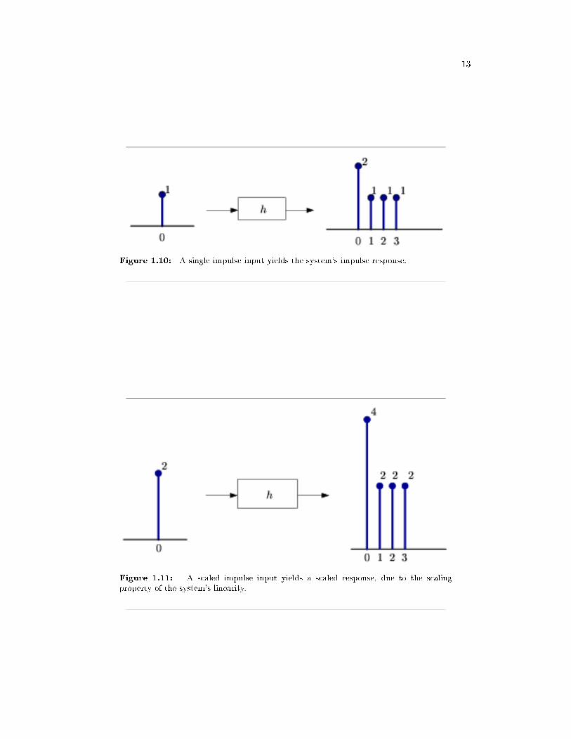
x [n] ∗ h [n] = h [n] ∗ x [n] (1.10)For more information on the characteristics of convolution, read about the Properties ofConvolution8.1.5.3 DerivationWe know that any discrete-time signal can be represented by a summation of scaled andshifted discrete-time impulses. Since we are assuming the system to be linear and time-invariant, it would seem to reason that an input signal comprised of the sum of scaled andshifted impulses would give rise to an output comprised of a sum of scaled and shiftedimpulse responses. This is exactly what occurs in convolution. Below we present a morerigorous and mathematical look at the derivation:
Letting H be a DT LTI system, we start with the following equation and work our waydown the convolution sum!
y [n] = H [x [n]]= H
[∑∞k=−∞ (x [k] δ [n− k])
]=
∑∞k=−∞ (H [x [k] δ [n− k]])
=∑∞
k=−∞ (x [k]H [δ [n− k]])=
∑∞k=−∞ (x [k]h [n− k])
(1.11)
Let us take a quick look at the steps taken in the above derivation. After our initial equation,we using the DT sifting property9 to rewrite the function, x [n], as a sum of the functiontimes the unit impulse. Next, we can move around the H operator and the summationbecause H [Ω] is a linear, DT system. Because of this linearity and the fact that x [k] is aconstant, we can pull the previous mentioned constant out and simply multiply it by H [Ω].Finally, we use the fact that H [Ω] is time invariant in order to reach our nal state - theconvolution sum!
A quick graphical example may help in demonstrating why convolution works.1.5.4 Convolution Through Time (A Graphical Approach)In this section we will develop a second graphical interpretation of discrete-time convolution.We will begin this by writing the convolution sum allowing x to be a causal, length-m signal
8http://cnx.org/content/m10088/latest/9http://cnx.org/content/m10059/latest/#sifting
13
Figure 1.10: A single impulse input yields the system's impulse response.
Figure 1.11: A scaled impulse input yields a scaled response, due to the scalingproperty of the system's linearity.

14 CHAPTER 1. FOUNDATIONS
Figure 1.12: We now use the time-invariance property of the system to show that adelayed input results in an output of the same shape, only delayed by the same amountas the input.
Figure 1.13: We now use the additivity portion of the linearity property of the systemto complete the picture. Since any discrete-time signal is just a sum of scaled and shifteddiscrete-time impulses, we can nd the output from knowing the input and the impulseresponse.

15
Figure 1.14: This is the end result that we are looking to nd.
and h to be a causal, length-k, LTI system. This gives us the nite summation,
y [n] =m−1∑l=0
(x [l]h [n− l]) (1.12)
Notice that for any given n we have a sum of the products of xl and a time-delayed h−l.This is to say that we multiply the terms of x by the terms of a time-reversed h and addthem up.
Going back to the previous example:What we are doing in the above demonstration is reversing the impulse response in time
and "walking it across" the input signal. Clearly, this yields the same result as scaling,shifting and summing impulse responses.
This approach of time-reversing, and sliding across is a common approach to presentingconvolution, since it demonstrates how convolution builds up an output through time.
1.6 Review of Linear AlgebraVector spaces are the principal object of study in linear algebra. A vector space is alwaysdened with respect to a eld of scalars.
1.6.1 FieldsA eld is a set F equipped with two operations, addition and mulitplication, and containingtwo special members 0 and 1 (0 6= 1), such that for all a, b, c ∈ F
1. (a) a + b ∈ F

16 CHAPTER 1. FOUNDATIONS
Figure 1.15: Here we reverse the impulse response, h , and begin its traverse at time0.
Figure 1.16: We continue the traverse. See that at time 1 , we are multiplying twoelements of the input signal by two elements of the impulse response.

17
Figure 1.17
(b) a + b = b + a
(c) (a + b) + c = a + (b + c)
(d) a + 0 = a
(e) there exists −a such that a + (−a) = 0
2. (a) ab ∈ F
(b) ab = ba
(c) (ab) c = a (bc)
(d) a · 1 = a
(e) there exists a−1 such that aa−1 = 1
3. a (b + c) = ab + ac
More concisely1. F is an abelian group under addition2. F is an abelian group under multiplication3. multiplication distributes over addition
1.6.1.1 ExamplesQ, R, C

18 CHAPTER 1. FOUNDATIONS
Figure 1.18: If we follow this through to one more step, n = 4, then we can see thatwe produce the same output as we saw in the initial example.

19
1.6.2 Vector SpacesLet F be a eld, and V a set. We say V is a vector space over F if there exist two operations,dened for all a ∈ F , u ∈ V and v ∈ V :• vector addition: (u, v) → u + v ∈ V
• scalar multiplication: (a,v) → av ∈ V
and if there exists an element denoted 0 ∈ V , such that the following hold for all a ∈ F ,b ∈ F , and u ∈ V , v ∈ V , and w ∈ V
1. (a) u + (v + w) = (u + v) + w
(b) u + v = v + u
(c) u + 0 = u
(d) there exists −u such that u + (−u) = 0
2. (a) a (u + v) = au + av
(b) (a + b)u = au + bu
(c) (ab)u = a (bu)
(d) 1 · u = u
More concisely,1. V is an abelian group under plus2. Natural properties of scalar multiplication
1.6.2.1 Examples• RN is a vector space over R
• CN is a vector space over C
• CN is a vector space over R
• RN is not a vector space over C
The elements of V are called vectors.
1.6.3 Euclidean SpaceThroughout this course we will think of a signal as a vector
x =
x1
x2...xN
=(
x1 x2 . . . xN
)T
The samples xi could be samples from a nite duration, continuous time signal, for ex-ample.
A signal will belong to one of two vector spaces:

20 CHAPTER 1. FOUNDATIONS
Figure 1.19: S is any line through the origin.
1.6.3.1 Real Euclidean spacex ∈ RN (over R)
1.6.3.2 Complex Euclidean spacex ∈ CN (over C)
1.6.4 SubspacesLet V be a vector space over F .
A subset S ⊆ V is called a subspace of V if S is a vector space over F in its own right.
Example 1.1:V = R2, F = R, S = any line though the origin.Are there other subspaces?Theorem 1.1:S ⊆ V is a subspace if and only if for all a ∈ F and b ∈ F and for all s ∈ S andt ∈ S, as + bt ∈ S
1.6.5 Linear IndependenceLet u1, . . . ,uk ∈ V .
We say that these vectors are linearly dependent if there exist scalars a1, . . . , ak ∈ Fsuch that
k∑i=1
(aiui) = 0 (1.13)
and at least one ai 6= 0.If Equation 1.13 only holds for the case a1 = · · · = ak = 0, we say that the vectors are
linearly independent.Example 1.2:

21
Figure 1.20: < S > is the xy-plane.
1
1−12
− 2
−230
+ 1
−57−2
= 0
so these vectors are linearly dependent in R3.
1.6.6 Spanning SetsConsider the subset S = v1, v2, . . . , vk. Dene the span of S
< S >≡ span (S) ≡
k∑
i=1
(aivi) |ai ∈ F
Fact: < S > is a subspace of V .Example 1.3:V = R3, F = R, S = v1, v2, v1 =
100
, v2 =
010
⇒ < S >= xy-plane.
1.6.6.1 AsideIf S is innite, the notions of linear independence and span are easily generalized:
We say S is linearly independent if, for every nite collection u1, . . . , uk ∈ S, (k arbitrary)we have
k∑i=1
(aiui) = 0⇒ ai = 0 ,
The span of S is< S >=
k∑
i=1
(aiui) |ai ∈ F ui ∈ S k < ∞
Note: In both denitions, we only consider nite sums.

22 CHAPTER 1. FOUNDATIONS
1.6.7 BasesA set B ⊆ V is called a basis for V over F if and only if
1. B is linearly independent2. < B >= V
Bases are of fundamental importance in signal processing. They allow us to decompose asignal into building blocks (basis vectors) that are often more easily understood.
Example 1.4:V = (real or complex) Euclidean space, RN or CN .
B = e1, . . . , eN ≡ standard basis
ei =
0...1...0
where the 1 is in the ith position.
Example 1.5:V = CN over C.
B = u1, . . . , uN
which is the DFT basis.
uk =
1
e−(j2π kN )
...e−(j2π k
N (N−1))
where j =
√−1.
1.6.7.1 Key FactIf B is a basis for V , then every v ∈ V can be written uniquely (up to order of terms) inthe form
v =N∑
i=1
(aivi)
where ai ∈ F and vi ∈ B.1.6.7.2 Other Facts• If S is a linearly independent set, then S can be extended to a basis.• If < S >= V , then S contains a basis.

23
1.6.8 DimensionLet V be a vector space with basis B. The dimension of V , denoted dim (V ), is the cardi-nality of B.
Theorem 1.2:Every vector space has a basis.Theorem 1.3:Every basis for a vector space has the same cardinality.⇒ dim (V ) is well-dened.If dim (V ) < ∞, we say V is nite dimensional.
1.6.8.1 Examples
vector space eld of scalars dimensionRN RCN CCN R
Every subspace is a vector space, and therefore has its own dimension.Example 1.6:Suppose S = u1, . . . , uk ⊆ V is a linearly independent set. Then
dim (< S >) =
Facts• If S is a subspace of V , then dim (S) ≤ dim (V ).• If dim (S) = dim (V ) < ∞, then S = V .
1.6.9 Direct SumsLet V be a vector space, and let S ⊆ V and T ⊆ V be subspaces.
We say V is the direct sum of S and T , written V = (S ⊕ T ), if and only if for everyv ∈ V , there exist unique s ∈ S and t ∈ T such that v = s + t.
If V = (S ⊕ T ), then T is called a complement of S.Example 1.7:
V = C ′ = leftf : R → R|f is continuousrightS = even funcitons inC ′
T = odd funcitons inC ′
f (t) =12
(f (t) + f (−t)) +12
(f (t)− f (−t))
If f = g + h = g′ + h′, g ∈ S and g′ ∈ S, h ∈ T and h′ ∈ T , then g − g′ = h′ − h isodd and even, which implies g = g′ and h = h′.

24 CHAPTER 1. FOUNDATIONS
1.6.9.1 Facts1. Every subspace has a complement2. V = (S ⊕ T ) if and only if
(a) S⋂
T = 0(b) < S, T >= V
3. If V = (S ⊕ T ), and dim (V ) < ∞, then dim (V ) = dim (S) + dim (T )
1.6.9.2 ProofsInvoke a basis.1.6.10 NormsLet V be a vector space over F . A norm is a mapping (V → F ), denoted by ‖ · ‖, such thatforall u ∈ V , v ∈ V , and λ ∈ F
1. ‖ u ‖> 0 if u 6= 0
2. ‖ λu ‖= |λ| ‖ u ‖
3. ‖ u + v ‖≤‖ u ‖ + ‖ v ‖
1.6.10.1 ExamplesEuclidean norms:
x ∈ RN :‖ x ‖=
(N∑
i=1
(xi
2)) 1
2
x ∈ CN :‖ x ‖=
(N∑
i=1
((|xi|)2
)) 12
1.6.10.2 Induced MetricEvery norm induces a metric on V
d (u,v) ≡‖ u− v ‖
which leads to a notion of "distance" between vectors.1.6.11 Inner productsLet V be a vector space over F , F = R or C. An inner product is a mapping V × V → F ,denoted · · ·, such that
1. v · v ≥ 0, and (v · v = 0 ⇔ v = 0)
2. u · v = v · u∗
3. au + bv · w = au · w + bv · w

25
1.6.11.1 ExamplesRN over R:
x · y = xT y =N∑
i=1
(xiyi)
CN over C:x · y = xHy =
N∑i=1
(xi∗yi)
If x = (x1, . . . , xN )T ∈ C, then
xH ≡
x1∗
...xN
∗
T
is called the "Hermitian," or "conjugate transpose" of x.1.6.12 Triangle InequalityIf we dene ‖ u ‖= u · u, then
‖ u + v ‖≤‖ u ‖ + ‖ v ‖
Hence, every inner product induces a norm.1.6.13 Cauchy-Schwarz InequalityFor all u ∈ V , v ∈ V ,
|u · v| ≤‖ u ‖‖ v ‖
In inner product spaces, we have a notion of the angle between two vectors:∠ (u,v) = arccos
(u · v
‖ u ‖‖ v ‖
)∈ [0, 2π)
1.6.14 Orthogonalityu and v are orthogonal if
u · v = 0
Notation: (u ⊥ v).If in addition ‖ u ‖=‖ v ‖= 1, we say u and v are orthonormal.In an orthogonal (orthonormal) set, each pair of vectors is orthogonal (orthonormal).
1.6.15 Orthonormal BasesAn Orthonormal basis is a basis vi such that
vi · vi = δij =
1 if i = j0 if i 6= j

26 CHAPTER 1. FOUNDATIONS
Figure 1.21: Orthogonal vectors in R2.
Example 1.8:The standard basis for RN or CN
Example 1.9:The normalized DFT basis
uk =1√N
1
e−(j2π kN )
...e−(j2π k
N (N−1))
1.6.16 Expansion CoecientsIf the representation of v with respect to vi is
v =∑
(aivi)
thenai = vi · v
1.6.17 Gram-SchmidtEvery inner product space has an orthonormal basis. Any (countable) basis can be madeorthogonal by the Gram-Schmidt orthogonalization process.1.6.18 Orthogonal ComplimentsLet S ⊆ V be a subspace. The orthogonal compliment S is
S⊥ = u |u ∈ V u · v = 0 v ∈ S ,
S⊥ is easily seen to be a subspace.If dim (v) < ∞, then V =
(S ⊕ S⊥
).

27
Aside: If dim (v) = ∞, then in order to have V =(S ⊕ S⊥
) we require V to bea Hilbert Space.
1.6.19 Linear TransformationsLoosely speaking, a linear transformation is a mapping from one vector space to anotherthat preserves vector space operations.
More precisely, let V , W be vector spaces over the same eld F . A linear transforma-tion is a mapping T : V → W such that
T (au + bv) = aT (u) + bT (v)
for all a ∈ F , b ∈ F and u ∈ V , v ∈ V .In this class we will be concerned with linear transformations between (real or complex)
Euclidean spaces, or subspaces thereof.
1.6.20 Imageimage (T ) = w |w ∈ W T (v) = wfor somev
1.6.21 NullspaceAlso known as the kernel:
ker (T ) = v |v ∈ V T (v) = 0
Both the image and the nullspace are easily seen to be subspaces.
1.6.22 Rankrank (T ) = dim (image (T ))
1.6.23 Nullitynull (T ) = dim (ker (T ))
1.6.24 Rank plus nullity theoremrank (T ) + null (T ) = dim (V )

28 CHAPTER 1. FOUNDATIONS
Figure 1.22
1.6.25 MatricesEvery linear transformation T has a matrix representation. If T : EN → EM , E = R orC, then T is represented by an M ×N matrix
A =
a11 . . . a1N... . . . ...aM1 . . . aMN
where (a1i, . . . , aMi)
T = T (ei) and ei = (0, . . . , 1, . . . , 0)T is the ith standard basis vector.Aside: A linear transformation can be represented with respect to any bases ofEN and EM , leading to a dierent A. We will always represent a linear transfor-mation using the standard bases.
1.6.26 Column spancolspan (A) =< A >= image (A)
1.6.27 DualityIf A : RN → RM , then
ker⊥ (A) = image(AT)
If A : CN → CM , thenker⊥ (A) = image
(AH)

29
1.6.28 InversesThe linear transformation/matrix A is invertible if and only if there exists a matrix B suchthat AB = BA = I (identity).
Only square matrices can be invertible.Theorem 1.4:Let A : FN → FN be linear, F = R or C. The following are equivalent:
1.A is invertible (nonsingular)2.rank (A) = N
3.null (A) = 0
4.detA 6= 0
5.The columns of A form a basis.If A−1 = AT (or AH in the complex case), we say A is orthogonal (or unitary).
1.7 Hilbert Spaces1.7.1 Hilbert SpacesA vector space S with a valid inner product10 dened on it is called an inner productspace, which is also a normed linear space. A Hilbert space is an inner product spacethat is complete with respect to the norm dened using the inner product. Hilbert spacesare named after David Hilbert11, who developed this idea through his studies of integralequations. We dene our valid norm using the inner product as:
‖ x ‖=√
x · x (1.14)Hilbert spaces are useful in studying and generalizing the concepts of Fourier expansion,Fourier transforms, and are very important to the study of quantum mechanics. Hilbertspaces are studied under the functional analysis branch of mathematics.1.7.1.1 Examples of Hilbert SpacesBelow we will list a few examples of Hilbert spaces12. You can verify that these are validinner products at home.• For Cn,
x · y = yT x =(
y0∗ y1
∗ . . . yn−1∗ )
x0
x1...xn−1
=n−1∑i=0
(xiyi∗)
• Space of nite energy complex functions: L2 (R)
f · g =∫ ∞
−∞f (t) g (t)∗dt
10http://cnx.org/content/m10755/latest/11http://www-history.mcs.st-andrews.ac.uk/history/Mathematicians/Hilbert.html12http://cnx.org/content/m10434/latest/

30 CHAPTER 1. FOUNDATIONS
• Space of square-summable sequences: `2 (Z)
x · y =∞∑
i=−∞
(x [i] y [i]∗
)
1.8 Signal Expansions1.8.1 Main IdeaWhen working with signals many times it is helpful to break up a signal into smaller, moremanageable parts. Hopefully by now you have been exposed to the concept of eigenvectors13and there use in decomposing a signal into one of its possible basis. By doing this we are ableto simplify our calculations of signals and systems through eigenfunctions of LTI systems14.
Now we would like to look at an alternative way to represent signals, through the useof orthonormal basis. We can think of orthonormal basis as a set of building blocks weuse to construct functions. We will build up the signal/vector as a weighted sum of basiselements.
Example 1.10:The complex sinusoids 1√
Tejω0nt for all −∞ < n < ∞ form an orthonormal basis
for L2 ([0, T ]).In our Fourier series15 equation, f (t) =
∑∞n=−∞
(cnejω0nt
), the cn are justanother representation of f (t).
note: For signals/vectors in a Hilbert Space16, the expansion coecients areeasy to nd.
1.8.2 Alternate RepresentationRecall our denition of a basis: A set of vectors bi in a vector space S is a basis if
1. The bi are linearly independent.2. The bi span17 S. That is, we can nd αi, where αi ∈ C (scalars) such that
x =∑
i
(αibi) , x ∈ S (1.15)
where x is a vector in S, α is a scalar in C, and b is a vector in S.Condition 2 in the above denition says we can decompose any vector in terms of the
bi. Condition 1 ensures that the decomposition is unique (think about this at home).note: The αi provide an alternate representation of x.
13http://cnx.org/content/m10736/latest/14http://cnx.org/content/m10500/latest/15http://cnx.org/content/m10496/latest/16http://cnx.org/content/m10755/latest/#sec217http://cnx.org/content/m10734/latest/#span_sec
31
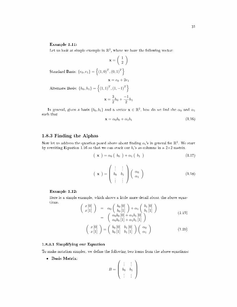
Example 1.11:Let us look at simple example in R2, where we have the following vector:
x =(
12
)Standard Basis: e0, e1 =
(1, 0)T
, (0, 1)T
x = e0 + 2e1
Alternate Basis: h0, h1 =
(1, 1)T, (1,−1)T
x =
32h0 +
−12
h1
In general, given a basis b0, b1 and a vector x ∈ R2, how do we nd the α0 and α1such thatx = α0b0 + α1b1 (1.16)
1.8.3 Finding the AlphasNow let us address the question posed above about nding αi's in general for R2. We startby rewriting Equation 1.16 so that we can stack our bi's as columns in a 2×2 matrix.(
x)
= α0
(b0
)+ α1
(b1
) (1.17)
(x)
=
... ...b0 b1... ...
( α0
α1
)(1.18)
Example 1.12:Here is a simple example, which shows a little more detail about the above equa-tions. (
x [0]x [1]
)= α0
(b0 [0]b0 [1]
)+ α1
(b1 [0]b1 [1]
)=
(α0b0 [0] + α1b1 [0]α0b0 [1] + α1b1 [1]
) (1.19)
(x [0]x [1]
)=(
b0 [0] b1 [0]b0 [1] b1 [1]
)(α0
α1
)(1.20)
1.8.3.1 Simplifying our EquationTo make notation simpler, we dene the following two items from the above equations:• Basis Matrix:
B =
... ...b0 b1... ...

32 CHAPTER 1. FOUNDATIONS
• Coecient Vector:α =
(α0
α1
)This gives us the following, concise equation:
x = Bα (1.21)which is equivalent to x =
∑1i=0 (αibi).
Example 1.13:Given a standard basis,
(10
),
(01
), then we have the following basis ma-
trix:B =
(0 11 0
)To get the αi's, we solve for the coecient vector in Equation 1.21
α = B−1x (1.22)Where B−1 is the inverse matrix18 of B.1.8.3.2 Examples
Example 1.14:Let us look at the standard basis rst and try to calculate α from it.
B =(
1 00 1
)= I
Where I is the identity matrix. In order to solve for α let us nd the inverse ofB rst (which is obviously very trivial in this case):
B−1 =(
1 00 1
)Therefore we get,
α = B−1x = x
Example 1.15:Let us look at a ever-so-slightly more complicated basis of
(11
),
(1−1
)=
h0, h1 Then our basis matrix and inverse basis matrix becomes:
B =(
1 11 −1
)
B−1 =(
12
12
12
−12
)18http://cnx.org/content/m2113/latest/

33
and for this example it is given thatx =
(32
)Now we solve for α
α = B−1x =(
12
12
12
−12
)(32
)=(
2.50.5
)and we get
x = 2.5h0 + 0.5h1
Exercise 1.1:Now we are given the following basis matrix and x:
b0, b1 =(
12
),
(30
)x =
(32
)For this problem, make a sketch of the bases and then represent x in terms of b0and b1.note: A change of basis simply looks at x from a "dierent perspective." B−1
transforms x from the standard basis to our new basis, b0, b1. Notice that thisis a totally mechanical procedure.
1.8.4 Extending the Dimension and SpaceWe can also extend all these ideas past just R2 and look at them in Rn and Cn. Thisprocedure extends naturally to higher (>2) dimensions. Given a basis b0, b1, . . . , bn−1 forRn, we want to nd α0, α1, . . . , αn−1 such that
x = α0b0 + α1b1 + · · ·+ αn−1bn−1 (1.23)Again, we will set up a basis matrix
B =(
b0 b1 b2 . . . bn−1
)where the columns equal the basis vectors and it will always be an n×n matrix (althoughthe above matrix does not appear to be square since we left terms in vector notation). Wecan then proceed to rewrite Equation 1.21
x =(
b0 b1 . . . bn−1
) α0...αn−1
= Bα
andα = B−1x
1.9 Fourier AnalysisFourier analysis is fundamental to understanding the behavior of signals and systems. Thisis a result of the fact that sinusoids are Eigenfunctions19 of linear, time-invariant (LTI)20
19http://cnx.org/content/m10500/latest/20http://cnx.org/content/m10084/latest/

34 CHAPTER 1. FOUNDATIONS
systems. This is to say that if we pass any particular sinusoid through a LTI system, we get ascaled version of that same sinusoid on the output. Then, since Fourier analysis allows us toredene the signals in terms of sinusoids, all we need to do is determine how any given systemeects all possible sinusoids (its transfer function21) and we have a complete understandingof the system. Furthermore, since we are able to dene the passage of sinusoids througha system as multiplication of that sinusoid by the transfer function at the same frequency,we can convert the passage of any signal through a system from convolution22 (in time) tomultiplication (in frequency). These ideas are what give Fourier analysis its power.
Now, after hopefully having sold you on the value of this method of analysis, we must ex-amine exactly what we mean by Fourier analysis. The four Fourier transforms that comprisethis analysis are the Fourier Series23, Continuous-Time Fourier Transform (Section 2.10),Discrete-Time Fourier Transform (Section 2.11) and Discrete Fourier Transform24. For thisdocument, we will view the Laplace Transform25 and Z-Transform (Section 4.3) as simplyextensions of the CTFT and DTFT respectively. All of these transforms act essentiallythe same way, by converting a signal in time to an equivalent signal in frequency (sinu-soids). However, depending on the nature of a specic signal i.e. whether it is nite- orinnite-length and whether it is discrete- or continuous-time) there is an appropriate trans-form to convert the signal into the frequency domain. Below is a table of the four Fouriertransforms and when each is appropriate. It also includes the relevant convolution for thespecied space.
Table of Fourier Representations
Transform Time Domain Frequency Domain ConvolutionContinuous-Time Fourier Series L2 ([0, T )) l2 (Z) Continuous-Time Circular
Continuous-Time Fourier Transform L2 (R) L2 (R) Continuous-Time LinearDiscrete-Time Fourier Transform l2 (Z) L2 ([0, 2π)) Discrete-Time Linear
Discrete Fourier Transform l2 ([0, N − 1]) l2 ([0, N − 1]) Discrete-Time Circular
1.10 Continuous-Time Fourier Transform (CTFT)1.10.1 IntroductionDue to the large number of continuous-time signals that are present, the Fourier series26provided us the rst glimpse of how me we may represent some of these signals in a generalmanner: as a superposition of a number of sinusoids. Now, we can look at a way torepresent continuous-time nonperiodic signals using the same idea of superposition. Belowwe will present the Continuous-Time Fourier Transform (CTFT), also referred to asjust the Fourier Transform (FT). Because the CTFT now deals with nonperiodic signals,we must now nd a way to include all frequencies in the general equations.1.10.1.1 EquationsContinuous-Time Fourier Transform
21http://cnx.org/content/m0028/latest/22http://cnx.org/content/m10088/latest/23http://cnx.org/content/m10097/latest/24http://cnx.org/content/m0502/latest/25http://cnx.org/content/m10110/latest/26http://cnx.org/content/m0039/latest/

35
Figure 1.23: Mapping L2 (R) in the time domain to L2 (R) in the frequency domain.
F (Ω) =∫ ∞
−∞f (t) e−(jΩt)dt (1.24)
Inverse CTFTf (t) =
12π
∫ ∞
−∞F (Ω) ejΩtdΩ (1.25)
warning: Do not be confused by notation - it is not uncommon to see the aboveformula written slightly dierent. One of the most common dierences amongmany professors is the way that the exponential is written. Above we used theradial frequency variable Ω in the exponential, where Ω = 2πf , but one will oftensee professors include the more explicit expression, j2πft, in the exponential. Clickhere27 for an overview of the notation used in Connexion's DSP modules.The above equations for the CTFT and its inverse come directly from the Fourier series
and our understanding of its coecients. For the CTFT we simply utilize integration ratherthan summation to be able to express the aperiodic signals. This should make sense sincefor the CTFT we are simply extending the ideas of the Fourier series to include nonperiodicsignals, and thus the entire frequency spectrum. Look at the Derivation of the FourierTransform28 for a more in depth look at this.1.10.2 Relevant SpacesThe Continuous-Time Fourier Transform maps innite-length, continuous-time signals inL2 to innite-length, continuous-frequency signals in L2. Review the Fourier Analysis (Sec-tion 2.9) for an overview of all the spaces used in Fourier analysis.
For more information on the characteristics of the CTFT, please look at the module onProperties of the Fourier Transform29.1.10.3 Example Problems
Exercise 1.2:Find the Fourier Transform (CTFT) of the function
f (t) =
e−(αt) if t ≥ 00 otherwise (1.26)
27http://cnx.org/content/m10161/latest/28http://cnx.org/content/m0046/latest/29http://cnx.org/content/m10100/latest/

36 CHAPTER 1. FOUNDATIONS
Figure 1.24: Mapping l2 (Z) in the time domain to L2 ([0, 2π)) in the frequency domain.
Exercise 1.3:Find the inverse Fourier transform of the square wave dened as
X (Ω) =
1 if |Ω| ≤ M0 otherwise (1.27)
1.11 Discrete-Time Fourier Transform (DTFT)Discrete-Time Fourier Transform
X (ω) =∞∑
n=−∞
(x (n) e−(jωn)
) (1.28)
Inverse Discrete-Time Fourier Transformx (n) =
12π
∫ 2π
0
X (ω) ejωndω (1.29)
1.11.1 Relevant SpacesThe Discrete-Time Fourier Transform 30maps innite-length, discrete-time signals in l2 tonite-length (or 2π-periodic), continuous-frequency signals in L2.
1.12 DFT as a Matrix Operation1.12.1 Matrix ReviewRecall:• Vectors in RN :
x =
x0
x1
. . .xN−1
, xi ∈ R
30http://cnx.org/content/m10247/latest/

37
• Vectors in CN :x =
x0
x1
. . .xN−1
, xi ∈ C
• Transposition:1. transpose:
xT =(
x0 x1 . . . xN−1
)2. conjugate:
xH =(
x0∗ x1
∗ . . . xN−1∗ )
• Inner product31:1. real:
xT y =N−1∑i=0
(xiyi)
2. complex:xHy =
N−1∑i=0
(xn∗yn)
• Matrix Multiplication:
Ax =
a00 a01 . . . a0,N−1
a10 a11 . . . a1,N−1... ... . . ....
aN−1,0 aN−1,1 . . . aN−1,N−1
x0
x1
. . .xN−1
=
y0
y1
. . .yN−1
yk =N−1∑n=0
(aknxn)
• Matrix Transposition:
AT =
a00 a10 . . . aN−1,0
a01 a11 . . . aN−1,1... ... . . ....
a0,N−1 a1,N−1 . . . aN−1,N−1
Matrix transposition involved simply swapping the rows with columns.
AH = AT ∗
The above equation is Hermitian transpose.[AT]kn
= Ank[AH]kn
= [A∗]nk
31http://cnx.org/content/m10755/latest/

38 CHAPTER 1. FOUNDATIONS
1.12.2 Representing DFT as Matrix OperationNow let's represent the DFT32 in vector-matrix notation.
x =
x [0]x [1]. . .
x [N − 1]
X =
X [0]X [1]. . .
X [N − 1]
∈ CN
Here x is the vector of time samples and X is the vector of DFT coecients. How are xand X related:
X [k] =N−1∑n=0
(x [n] e−(j 2π
N kn))
whereakn =
(e−(j 2π
N ))kn
= WNkn
soX = Wx
where X is the DFT vector, W is the matrix and x the time domain vector.Wkn =
(e−(j 2π
N ))kn
X = W
x [0]x [1]. . .
x [N − 1]
IDFT:
x [n] =1N
N−1∑k=0
(X [k]
(ej 2π
N
)nk)
where (ej 2π
N
)nk
= WNnk∗
WNnk∗ is the matrix Hermitian transpose. So,
x =1N
WHX
where x is the time vector, 1N WH is the inverse DFT matrix, and X is the DFT vector.
1.13 The FFT AlgorithmDenition 1: FFT(Fast Fourier Transform) An ecient computational algorithm for computingthe DFT33.
32http://cnx.org/content/m10249/latest/33http://cnx.org/content/m10249/latest/

39
Figure 1.25
Figure 1.26
1.13.1 The Fast Fourier Transform FFTDFT can be expensive to compute directly
X [k] =N−1∑n=0
(x [n] e−(j2π k
N n))
, 0 ≤ k ≤ N − 1
For each k, we must execute:• N complex multiplies• N − 1 complex adds
The total cost of direct computation of an N -point DFT is• N2 complex multiplies• N (N − 1) complex adds
How many adds and mults of real numbers are required?This " O
(N2)" computation rapidly gets out of hand, as N gets large:
N 1 10 100 1000 106
N2 1 100 10,000 106 1012
The FFT provides us with a much more ecient way of computing the DFT. The FFTrequires only " O (N logN)" computations to compute the N -point DFT.
N 10 100 1000 106
N2 100 10,000 106 1012
N log10N 10 200 3000 6× 10⁶
How long is 1012µsec? More than 10 days! How long is 6× 10⁶µsec?The FFT and digital computers revolutionized DSP (1960 - 1980).

40 CHAPTER 1. FOUNDATIONS
1.13.2 How does the FFT work?• The FFT exploits the symmetries of the complex exponentials WN
kn = e−(j 2πN kn)
• WNkn are called "twiddle factors"
Symmetry 1.1: Complex Conjugate SymmetryWN
k(N−n) = WN−(kn) = WN
kn∗
e−(j2π kN (N−n)) = ej2π k
N n = e−(j2π kN n)∗
Symmetry 1.2: Periodicity in n and kWN
kn = WNk(N+n) = WN
(k+N)n
e−(j 2πN kn) = e−(j 2π
N k(N+n)) = e−(j 2πN (k+N)n)
WN = e−(j 2πN )
1.13.3 Decimation in Time FFT• Just one of many dierent FFT algorithms• The idea is to build a DFT out of smaller and smaller DFTs by decomposing x [n] into
smaller and smaller subsequences.• Assume N = 2m (a power of 2)
1.13.3.1 DerivationN is even, so we can complete X [k] by separating x [n] into two subsequences each of lengthN2 .
x [n] →
N2 if n = evenN2 if n = odd
X [k] =N−1∑n=0
(x [n]WN
kn)
, 0 ≤ k ≤ N − 1
X [k] =∑(
x [n]WNkn)
+∑(
x [n]WNkn)
where 0 ≤ r ≤ N2 − 1. So
X [k] =∑N
2 −1r=0
(x [2r]WN
2kr)
+∑N
2 −1r=0
(x [2r + 1]WN
(2r+1)k)
=∑N
2 −1r=0
(x [2r]
(WN
2)kr)
+ WNk∑N
2 −1r=0
(x [2r + 1]
(WN
2)kr) (1.30)
where WN2 = e−(j 2π
N 2) = e−
„j 2π
N2
«= WN
2. So
X [k] =
N2 −1∑r=0
(x [2r]WN
2
kr)
+ WNk
N2 −1∑r=0
(x [2r + 1]WN
2
kr)

41
where∑N2 −1
r=0
(x [2r]WN
2
kr) is N
2 -point DFT of even samples ( G [k]) and∑N2 −1
r=0
(x [2r + 1]WN
2
kr)
is N2 -point DFT of odd samples ( H [k]).
X [k] = G [k] + WNkH [k] , 0 ≤ k ≤ N − 1
Decomposition of an N -point DFT as a sum of 2 N2 -point DFTs.Why would we want to do this? Because it is more ecient!
Recall: Cost to compute an N -point DFT is approximately N2 complex multsand adds.
But decomposition into 2 N2 -point DFTs + combination requires only(
N
2
)2
+(
N
2
)2
+ N =N2
2+ N
where the rst part is the number of complex mults and adds for N2 -point DFT, G [k]. The
second part is the number of complex mults and adds for N2 -point DFT, H [k]. The third
part is the number of complex mults and adds for combination. And the total is N2
2 + Ncomplex mults and adds.
Example 1.16: SavingsFor N = 1000,
N2 = 106
N2
2+ N =
106
2+ 1000
Because 1000 is small compared to 500,000,N2
2+ N ≈ 106
2
So why stop here?! Keep decomposing. Break each of the N2 -point DFTs into two
N4 -point DFTs, etc., ....We can keep decomposing:
N
21=
N
2,N
4,N
8, . . . ,
N
2m−1,
N
2m
= 1
wherem = log2N = times
Computational cost: N -pt DFT [U+F577] two N2 -pt DFTs. The cost is N2 → 2
(N2
)2+N .
So replacing each N2 -pt DFT with two N
4 -pt DFTs will reduce cost to
2
(2(
N
4
)2
+N
2
)+ N = 4
(N
4
)2
+ 2N =N2
22+ 2N =
N2
2p+ pN
As we keep going p = 3, 4, . . . ,m, where m = log2N . We get the costN2
2log2N+ N log2N =
N2
N+ N log2N = N + N log2N
N + N log2N is the total number of complex adds and mults.For large N , cost ≈ N log2N or " O (N log2N)", since (N log2N N) for large N .Note: Weird order of time samples

42 CHAPTER 1. FOUNDATIONS
Figure 1.27: N = 8 point FFT. Summing nodes Wnk twiddle multiplication factors.
Figure 1.28: This is called "butteries."
Solutions to Exercises in Chapter 1Solution to Exercise 1.1:In order to represent x in terms of b0 and b1 we will follow the same steps we used in theabove example.
B =(
1 23 0
)
B−1 =(
0 12
13
−16
)
α = B−1x =(
123
)And now we can write x in terms of b0 and b1.
x = b0 +23b1
And we can easily substitute in our known values of b0 and b1 to verify our results.Solution to Exercise 1.2:In order to calculate the Fourier transform, all we need to use is Equation 1.24, complexexponentials34, and basic calculus.
F (Ω) =∫∞−∞ f (t) e−(jΩt)dt
=∫∞0
e−(αt)e−(jΩt)dt=
∫∞0
e(−t)(α+jΩ)dt= 0− −1
α+jΩ
(1.31)
F (Ω) =1
α + jΩ(1.32)
34http://cnx.org/content/m10060/latest/

43
Solution to Exercise 1.3:Here we will use Equation 1.25 to nd the inverse FT given that t 6= 0.
x (t) = 12π
∫M
−MejΩtdΩ
= 12π ejΩt|Ω,Ω=ejw
= 1πt sin (Mt)
(1.33)
x (t) =M
π
(sinc
Mt
π
)(1.34)

44 CHAPTER 1. FOUNDATIONS

Chapter 2
Sampling and Frequency Analysis
2.1 IntroductionContents of Sampling chapter• Introduction(Current module)• Proof (Section 3.2)• Illustrations (Section 3.3)• Matlab Example (Section 3.4)• Hold operation1• System view (Section 3.5)• Aliasing applet2• Exercises3• Table of formulas4
2.1.1 Why sample?This section introduces sampling. Sampling is the necessary fundament for all digital signalprocessing and communication. Sampling can be dened as the process of measuring ananalog signal at distinct points.
Digital representation of analog signals oers advantages in terms of• robustness towards noise, meaning we can send more bits/s• use of exible processing equipment, in particular the computer• more reliable processing equipment• easier to adapt complex algorithms1http://cnx.org/content/m11458/latest/2http://cnx.org/content/m11448/latest/3http://cnx.org/content/m11442/latest/4http://cnx.org/content/m11450/latest/
45

46 CHAPTER 2. SAMPLING AND FREQUENCY ANALYSIS
Figure 2.1: Claude Elwood Shannon (1916-2001)
2.1.2 Claude E. ShannonClaude Shannon5 has been called the father of information theory, mainly due to his land-mark papers on the "Mathematical theory of communication"6. Harry Nyquist7 was therst to state the sampling theorem in 1928, but it was not proven until Shannon proved it21 years later in the paper "Communications in the presence of noise"8.
2.1.3 NotationIn this chapter we will be using the following notation• Original analog signal x (t)
• Sampling frequency Fs
• Sampling interval Ts (Note that: Fs = 1Ts)
• Sampled signal xs (n). (Note that xs (n) = x (nTs))• Real angular frequency Ω
• Digital angular frequency ω. (Note that: ω = ΩTs)
2.1.4 The Sampling TheoremThe Sampling theorem: When sampling an analog signal the sampling fre-quency must be greater than twice the highest frequency component of the analogsignal to be able to reconstruct the original signal from the sampled version.Finished? Have at look at: Proof (Section 3.2); Illustrations (Section 3.3); Matlab Exam-
ple (Section 3.4); Aliasing applet9; Hold operation10; System view (Section 3.5); Exercises11
2.2 ProofSampling theorem: In order to recover the signal x (t) from it's samples exactly,it is necessary to sample x (t) at a rate greater than twice it's highest frequencycomponent.
5http://www.research.att.com/∼njas/doc/ces5.html6http://cm.bell-labs.com/cm/ms/what/shannonday/shannon1948.pdf7http://www.wikipedia.org/wiki/Harry_Nyquist8http://www.stanford.edu/class/ee104/shannonpaper.pdf9http://cnx.org/content/m11448/latest/10http://cnx.org/content/m11458/latest/11http://cnx.org/content/m11442/latest/

47
2.2.1 IntroductionAs mentioned earlier (pg 45), sampling is the necessary fundament when we want to applydigital signal processing on analog signals.
Here we present the proof of the sampling theorem. The proof is divided in two. Firstwe nd an expression for the spectrum of the signal resulting from sampling the originalsignal x (t). Next we show that the signal x (t) can be recovered from the samples. Oftenit is easier using the frequency domain when carrying out a proof, and this is also the casehere.Key points in the proof• We nd an equation (Equation 2.8) for the spectrum of the sampled signal• We nd a simple method to reconstruct (Equation 2.14) the original signal• The sampled signal has a periodic spectrum...• ...and the period is 2πFs
2.2.2 Proof part 1 - Spectral considerationsBy sampling x (t) every Ts second we obtain xs (n). The inverse fourier transform of thistime discrete signal12 is
xs (n) =12π
∫ π
−π
Xs
(ejω)ejωndω (2.1)
For convenience we express the equation in terms of the real angular frequency Ω usingω = ΩTs. We then obtain
xs (n) =Ts
2π
∫ πTs
−πTs
Xs
(ejΩTs
)ejΩTsndΩ (2.2)
The inverse fourier transform of a continuous signal isx (t) =
12π
∫ ∞
−∞X (jΩ) ejΩtdΩ (2.3)
From this equation we nd an expression for x (nTs)
x (nTs) =12π
∫ ∞
−∞X (jΩ) ejΩnTsdΩ (2.4)
To account for the dierence in region of integration we split the integration in Equation 2.4into subintervals of length 2π
Tsand then take the sum over the resulting integrals to obtain
the complete area.
x (nTs) =12π
∞∑k=−∞
(∫ (2k+1)πTs
(2k−1)πTs
X (jΩ) ejΩnTsdΩ
)(2.5)
Then we change the integration variable, setting Ω = η + 2πkTs
x (nTs) =12π
∞∑k=−∞
(∫ πTs
−πTs
X
(j
(η +
2πk
Ts
))ej(η+ 2πk
Ts)nTsdη
)(2.6)
12http://cnx.org/content/m11476/latest/

48 CHAPTER 2. SAMPLING AND FREQUENCY ANALYSIS
We obtain the nal form by observing that ej2πkn = 1, reinserting η = Ω and multiplyingby Ts
Ts
x (nTs) =Ts
2π
∫ πTs
−πTs
∞∑k=−∞
(1Ts
X
(j
(Ω +
2πk
Ts
))ejΩnTs
)dΩ (2.7)
To make xs (n) = x (nTs) for all values of n, the integrands in Equation 2.2 and Equation 2.7have to agreee, that is
Xs
(ejΩTs
)=
1Ts
∞∑k=−∞
(X
(j
(Ω +
2πk
Ts
)))(2.8)
This is a central result. We see that the digital spectrum consists of a sum of shifted versionsof the original, analog spectrum. Observe the periodicity!
We can also express this relation in terms of the digital angular frequency ω = ΩTs
Xs
(ejω)
=1Ts
∞∑k=−∞
(X
(jω + 2πk
Ts
))(2.9)
This concludes the rst part of the proof. Now we want to nd a reconstruction formula,so that we can recover x (t) from xs (n).2.2.3 Proof part II - Signal reconstructionFor a bandlimited (Figure 2.3) signal the inverse fourier transform is
x (t) =12π
∫ πTs
−πTs
X (jΩ) ejΩtdΩ (2.10)
In the interval we are integrating we have: Xs
(ejΩTs
)= X(jΩ)
Ts. Substituting this relation
into Equation 2.10 we getx (t) =
Ts
2π
∫ πTs
−πTs
Xs
(ejΩTs
)ejΩtdΩ (2.11)
Using the DTFT13 relation for Xs
(ejΩTs
) we havex (t) =
Ts
2π
∫ πTs
−πTs
∞∑n=−∞
(xs (n) e−(jΩnTs)ejΩt
)dΩ (2.12)
Interchanging integration and summation (under the assumption of convergence) leads to
x (t) =Ts
2π
∞∑n=−∞
(xs (n)
∫ πTs
−πTs
ejΩ(t−nTs)dΩ
)(2.13)
Finally we perform the integration and arrive at the important reconstruction formula
x (t) =∞∑
n=−∞
xs (n)sin(
πTs
(t− nTs))
πTs
(t− nTs)
(2.14)
(Thanks to R.Loos for pointing out an error in the proof.)13http://cnx.org/content/m11450/latest/

49
2.2.4 Summaryspectrum sampled signal: Xs
(ejΩTs
)= 1
Ts
∑∞k=−∞
(X(j(Ω + 2πk
Ts
)))
Reconstruction formula: x (t) =∑∞
n=−∞
(xs (n)
sin( πTs
(t−nTs))π
Ts(t−nTs)
)Go to Introduction (Section 3.1); Illustrations (Section 3.3); Matlab Example (Sec-
tion 3.4); Hold operation14; Aliasing applet15; System view (Section 3.5); Exercises16 ?
2.3 IllustrationsIn this module we illustrate the processes involved in sampling and reconstruction. To seehow all these processes work together as a whole, take a look at the system view (Section 3.5).In Sampling and reconstruction with Matlab (Section 3.4) we provide a Matlab script fordownload. The matlab script shows the process of sampling and reconstruction live.
2.3.1 Basic examplesExample 2.1:To sample an analog signal with 3000 Hz as the highest frequency componentrequires sampling at 6000 Hz or above.
Example 2.2:The sampling theorem can also be applied in two dimensions, i.e. for image analy-sis. A 2D sampling theorem has a simple physical interpretation in image analysis:Choose the sampling interval such that it is less than or equal to half of the smallestinteresting detail in the image.
2.3.2 The process of samplingWe start o with an analog signal. This can for example be the sound coming from yourstereo at home or your friend talking.
The signal is then sampled uniformly. Uniform sampling implies that we sample everyTs seconds. In Figure 2.2 we see an analog signal. The analog signal has been sampledat times t = nTs. In signal processing it is often more convenient and easier to workin the frequency domain. So let's look at at the signal in frequency domain, Figure 2.3.For illustration purposes we take the frequency content of the signal as a triangle. (If youFourier transform the signal in Figure 2.2 you will not get such a nice triangle.) Notice thatthe signal in Figure 2.3 is bandlimited. We can see that the signal is bandlimited becauseX (jΩ) is zero outside the interval [−Ωg,Ωg]. Equivalentely we can state that the signal hasno angular frequencies above Ωg, corresponding to no frequencies above Fg = Ωg
2π .Now let's take a look at the sampled signal in the frequency domain. While proving(Section 3.2) the sampling theorem we found the the spectrum of the sampled signal consists
14http://cnx.org/content/m11458/latest/15http://cnx.org/content/m11448/latest/16http://cnx.org/content/m11442/latest/

50 CHAPTER 2. SAMPLING AND FREQUENCY ANALYSIS
Figure 2.2: Analog signal, samples are marked with dots.
Figure 2.3: The spectrum X (jΩ).
51
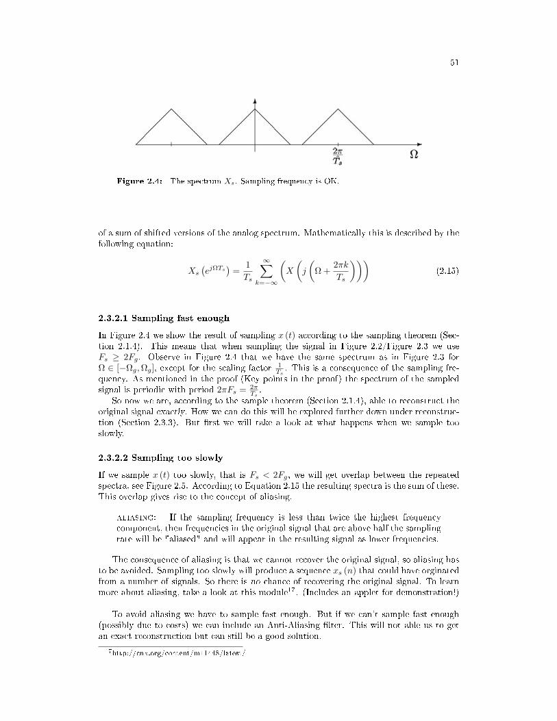
Figure 2.4: The spectrum Xs. Sampling frequency is OK.
of a sum of shifted versions of the analog spectrum. Mathematically this is described by thefollowing equation:
Xs
(ejΩTs
)=
1Ts
∞∑k=−∞
(X
(j
(Ω +
2πk
Ts
)))(2.15)
2.3.2.1 Sampling fast enoughIn Figure 2.4 we show the result of sampling x (t) according to the sampling theorem (Sec-tion 2.1.4). This means that when sampling the signal in Figure 2.2/Figure 2.3 we useFs ≥ 2Fg. Observe in Figure 2.4 that we have the same spectrum as in Figure 2.3 forΩ ∈ [−Ωg,Ωg], except for the scaling factor 1
Ts. This is a consequence of the sampling fre-
quency. As mentioned in the proof (Key points in the proof) the spectrum of the sampledsignal is periodic with period 2πFs = 2π
Ts.
So now we are, according to the sample theorem (Section 2.1.4), able to reconstruct theoriginal signal exactly. How we can do this will be explored further down under reconstruc-tion (Section 2.3.3). But rst we will take a look at what happens when we sample tooslowly.2.3.2.2 Sampling too slowlyIf we sample x (t) too slowly, that is Fs < 2Fg, we will get overlap between the repeatedspectra, see Figure 2.5. According to Equation 2.15 the resulting spectra is the sum of these.This overlap gives rise to the concept of aliasing.
aliasing: If the sampling frequency is less than twice the highest frequencycomponent, then frequencies in the original signal that are above half the samplingrate will be "aliased" and will appear in the resulting signal as lower frequencies.The consequence of aliasing is that we cannot recover the original signal, so aliasing has
to be avoided. Sampling too slowly will produce a sequence xs (n) that could have orginatedfrom a number of signals. So there is no chance of recovering the original signal. To learnmore about aliasing, take a look at this module17. (Includes an applet for demonstration!)
To avoid aliasing we have to sample fast enough. But if we can't sample fast enough(possibly due to costs) we can include an Anti-Aliasing lter. This will not able us to getan exact reconstruction but can still be a good solution.
17http://cnx.org/content/m11448/latest/

52 CHAPTER 2. SAMPLING AND FREQUENCY ANALYSIS
Figure 2.5: The spectrum Xs. Sampling frequency is too low.
Anti-Aliasing filter: Typically a low-pass lter that is applied before sam-pling to ensure that no components with frequencies greater than half the samplefrequency remain.
Example 2.3:The stagecoach eectIn older western movies you can observe aliasing on a stagecoach when it startsto roll. At rst the spokes appear to turn forward, but as the stagecoach increaseits speed the spokes appear to turn backward. This comes from the fact that thesampling rate, here the number of frames per second, is too low. We can vieweach frame as a sample of an image that is changing continuously in time. (Appletillustrating the stagecoach eect18)
2.3.3 ReconstructionGiven the signal in Figure 2.4 we want to recover the original signal, but the question ishow?
When there is no overlapping in the spectrum, the spectral component given by k = 0(see Equation 2.15),is equal to the spectrum of the analog signal. This oers an oppurtunityto use a simple reconstruction process. Remember what you have learned about ltering.What we want is to change signal in Figure 2.4 into that of Figure 2.3. To achieve this wehave to remove all the extra components generated in the sampling process. To remove theextra components we apply an ideal analog low-pass lter as shown in Figure 2.6 As we seethe ideal lter is rectangular in the frequency domain. A rectangle in the frequency domaincorresponds to a sinc19 function in time domain (and vice versa).
Then we have reconstructed the original spectrum, and as we know if two signals areidentical in the frequency domain, they are also identical in the time domain. End ofreconstruction.
2.3.4 ConclusionsThe Shannon sampling theorem requires that the input signal prior to sampling is band-limited to at most half the sampling frequency. Under this condition the samples give an
18http://owers.ofthenight.org/wagonWheel/wagonWheel.html19http://ccrma-www.stanford.edu/∼jos/Interpolation/sinc_function.html

53
Figure 2.6: H (jΩ) The ideal reconstruction lter.
exact signal representation. It is truly remarkable that such a broad and useful class signalscan be represented that easily!
We also looked into the problem of reconstructing the signals form its samples. Againthe simplicity of the principle is striking: linear ltering by an ideal low-pass lter will dothe job. However, the ideal lter is impossible to create, but that is another story...
Go to? Introduction (Section 3.1); Proof (Section 3.2); Illustrations (Section 3.3); MatlabExample (Section 3.4); Aliasing applet20; Hold operation21; System view (Section 3.5);Exercises22
2.4 Sampling and Reconstruction with Matlab2.4.1 Matlab lesSamprecon.m23
Introduction (Section 3.1); Proof (Section 3.2); Illustrations (Section 3.3); Aliasing ap-plet24; Hold operation (Section 3.4); System view (Section 3.5); Exercises25
2.5 Systems View of Sampling and Reconstruction2.5.1 Ideal reconstruction systemFigure 2.7 shows the ideal reconstruction system based on the results of the Samplingtheorem proof (Section 3.2).
Figure 2.7 consists of a sampling device which produces a time-discrete sequence xs (n).The reconstruction lter, h (t), is an ideal analog sinc26 lter, with h (t) = sinc
(t
Ts
). Wecan't apply the time-discrete sequence xs (n) directly to the analog lter h (t). To solvethis problem we turn the sequence into an analog signal using delta functions27. Thus wewrite xs (t) =
∑∞n=−∞ (xs (n) δ (t− nT )). But when will the system produce an output
x (t) = x (t)? According to the sampling theorem (Section 2.1.4) we have x (t) = x (t) whenthe sampling frequency, Fs, is at least twice the highest frequency component of x (t).
20http://cnx.org/content/m11448/latest/21http://cnx.org/content/m11458/latest/22http://cnx.org/content/m11442/latest/23http://cnx.rice.edu/content/m11549/latest/Samprecon.m24http://cnx.org/content/m11448/latest/25http://cnx.org/content/m11442/latest/26http://ccrma-www.stanford.edu/∼jos/Interpolation/sinc_function.html27http://cnx.org/content/m11450/latest/

54 CHAPTER 2. SAMPLING AND FREQUENCY ANALYSIS
Figure 2.7: Ideal reconstruction system
Figure 2.8: Ideal reconstruction system with anti-aliasing lter (pg 51)
2.5.2 Ideal system including anti-aliasingTo be sure that the reconstructed signal is free of aliasing it is customary to apply a lowpasslter, an anti-aliasing lter (pg 51), before sampling as shown in Figure 2.8. Again weask the question of when the system will produce an output x (t) = s (t)? If the signal isentirely conned within the passband of the lowpass lter we will get perfect reconstructionif Fs is high enough.
But if the anti-aliasing lter removes the "higher" frequencies, (which in fact is the jobof the anti-aliasing lter), we will never be able to exactly reconstruct the original signal,s (t). If we sample fast enough we can reconstruct x (t), which in most cases is satisfying.
The reconstructed signal, x (t), will not have aliased frequencies. This is essential forfurther use of the signal.
2.5.3 Reconstruction with hold operationTo make our reconstruction system realizable there are many things to look into. Amongthem are the fact that any practical reconstruction system must input nite length pulsesinto the reconstruction lter. This can be accomplished by the hold operation28. To alleviatethe distortion caused by the hold opeator we apply the output from the hold device to acompensator. The compensation can be as accurate as we wish, this is cost and applicationconsideration. By the use of the hold component the reconstruction will not be exact,but as mentioned above we can get as close as we want. Introduction (Section 3.1); Proof(Section 3.2); Illustrations (Section 3.3); Matlab example (Section 3.4); Hold operation30;
28http://cnx.org/content/m11458/latest/30http://cnx.org/content/m11458/latest/
Figure 2.9: More practical reconstruction system with a hold component29

55
Aliasing applet31; Exercises32
2.6 Sampling CT Signals: A Frequency Domain Perspec-tive2.6.1 Understanding Sampling in the Frequency DomainWe want to relate xc (t) directly to x [n]. Compute the CTFT of
xs (t) =∞∑
n=−∞(xc (nT ) δ (t− nT ))
Xs (Ω) =∫∞−∞
(∑∞n=−∞ (xc (nT ) δ (t− nT ))
)e(−j)Ωtdt
=∑∞
n=−∞
(xc (nT )
∫∞−∞ δ (t− nT ) e(−j)Ωtdt
)=
∑∞n=−∞
(x [n] e(−j)ΩnT
)=
∑∞n=−∞
(x [n] e(−j)ωn
)= X (ω)
(2.16)
where ω ≡ ΩT and X (ω) is the DTFT of x [n].Recall:
Xs (Ω) =1T
∞∑k=−∞
(Xc (Ω− kΩs))
X (ω) = 1T
∑∞k=−∞ (Xc (Ω− kΩs))
= 1T
∑∞k=−∞
(Xc
(ω−2πk
T
)) (2.17)where this last part is 2π-periodic.2.6.1.1 Sampling
Example 2.4: SpeechSpeech is intelligible if bandlimited by a CT lowpass lter to the band ±4 kHz.We can sample speech as slowly as _____?
2.6.2 Relating x[n] to sampled x(t)Recall the following equality:
xs (t) =∑
n
(x (nT ) δ (t− nT ))
Recall the CTFT relation: (x (αt) ↔ 1
αX
(Ωα
))(2.18)
where α is a scaling of time and 1α is a scaling in frequency.
Xs (Ω) ≡ X (ΩT ) (2.19)31http://cnx.org/content/m11448/latest/32http://cnx.org/content/m11442/latest/

56 CHAPTER 2. SAMPLING AND FREQUENCY ANALYSIS
Figure 2.10
Figure 2.11

57
Figure 2.12: Note that there is no mention of T or Ωs!
2.7 The DFT: Frequency Domain with a Computer Anal-ysis2.7.1 IntroductionWe just covered ideal (and non-ideal) (time) sampling of CT signals (Section 3.6). Thisenabled DT signal processing solutions for CT applications (Figure 2.14):
Much of the theoretical analysis of such systems relied on frequency domain representa-tions. How do we carry out these frequency domain analysis on the computer? Recall thefollowing relationships:
x [n] DTFT↔ X (ω)
x (t) CTFT↔ X (Ω)
where ω and Ω are continuous frequency variables.
2.7.1.1 Sampling DTFTConsider the DTFT of a discrete-time (DT) signal x [n]. Assume x [n] is of nite durationN ( i.e., an N -point signal).
X (ω) =N−1∑n=0
(x [n] e(−j)ωn
) (2.20)
where X (ω) is the continuous function that is indexed by the real-valued parameter −π ≤ω ≤ π. The other function, x [n], is a discrete function that is indexed by integers.

58 CHAPTER 2. SAMPLING AND FREQUENCY ANALYSIS
Figure 2.13
Figure 2.14

59
Finite Duration DT Signal
Figure 2.15
Sample X(ω)
Figure 2.16
We want to work with X (ω) on a computer. Why not just sample X (ω)?X [k] = X
(2πN k)
=∑N−1
n=0
(x [n] e(−j)2π k
N n) (2.21)
In Equation 2.21 we sampled at ω = 2πN k where k = 0, 1, . . . , N − 1 and X [k] for k =
0, . . . , N − 1 is called the Discrete Fourier Transform (DFT) of x [n].Example 2.5:The DTFT of the image in Figure 2.15 is written as follows:
X (ω) =N−1∑n=0
(x [n] e(−j)ωn
) (2.22)
where ω is any 2π-interval, for example −π ≤ ω ≤ π.where again we sampled at ω = 2π
N k where k = 0, 1, . . . ,M − 1. For example,we take
M = 10
. In the following section (Section 2.7.1.1.1) we will discuss in more detail how weshould choose M , the number of samples in the 2π interval.(This is precisely how we would plot X (ω) in Matlab.)
2.7.1.1.1 Choosing M2.7.1.1.1.1 Case 1Given N (length of x [n]), choose (M N) to obtain a dense sampling of the DTFT (Fig-ure 2.17):2.7.1.1.1.2 Case 2Choose M as small as possible (to minimize the amount of computation).
In general, we require M ≥ N in order to represent all information inx [n] , n = 0, . . . , N − 1

60 CHAPTER 2. SAMPLING AND FREQUENCY ANALYSIS
Figure 2.17
Let's concentrate on M = N :x [n] DFT↔ X [k]
for n = 0, . . . , N − 1 and k = 0, . . . , N − 1
numbers ↔ N numbers
2.7.2 Discrete Fourier Transform (DFT)Dene
X [k] ≡ X
(2πk
N
)(2.23)
where N = length (x [n]) and k = 0, . . . , N − 1. In this case, M = N .DFT
X [k] =N−1∑n=0
(x [n] e(−j)2π k
N n) (2.24)
Inverse DFT (IDFT)
x [n] =1N
N−1∑k=0
(X [k] ej2π k
N n) (2.25)
2.7.2.1 InterpretationRepresent x [n] in terms of a sum of N complex sinusoids33 of amplitudes X [k] and frequen-cies
ωk =2πk
N, k ∈ 0, . . . , N − 1
Think: Fourier Series with fundamental frequency 2πN
33http://cnx.org/content/m10060/latest/

61
Figure 2.18
2.7.2.1.1 Remark 1IDFT treats x [n] as though it were N -periodic.
x [n] =1N
N−1∑k=0
(X [k] ej2π k
N n) (2.26)
where n ∈ 0, . . . , N − 1
Exercise 2.1:What about other values of n?
2.7.2.1.2 Remark 2Proof that the IDFT inverts the DFT for n ∈ 0, . . . , N − 1
1N
∑N−1k=0
(X [k] ej2π k
N n)
= 1N
∑N−1k=0
(∑N−1m=0
(x [m] e(−j)2π k
N mej2π kN n))
= ???(2.27)
Example 2.6: Computing DFTGiven the following discrete-time signal (Figure 2.18) with N = 4, we will computethe DFT using two dierent methods (the DFT Formula and Sample DTFT):
1.DFT FormulaX [k] =
∑N−1n=0
(x [n] e(−j)2π k
N n)
= 1 + e(−j)2π k4 + e(−j)2π k
4 2 + e(−j)2π k4 3
= 1 + e(−j) π2 k + e(−j)πk + e(−j) 3
2 πk
(2.28)
Using the above equation, we can solve and get the following results:x [0] = 4
x [1] = 0
x [2] = 0
x [3] = 0

62 CHAPTER 2. SAMPLING AND FREQUENCY ANALYSIS
Figure 2.19
2.Sample DTFT. Using the same gure, Figure 2.18, we will take the DTFT ofthe signal and get the following equations:
X (ω) =∑3
n=0
(e(−j)ωn
)= 1−e(−j)4ω
1−e(−j)ω
= ???(2.29)
Our sample points will be:ωk =
2πk
4=
π
2k
where k = 0, 1, 2, 3 (Figure 2.19).
2.7.3 Periodicity of the DFTDFT X [k] consists of samples of DTFT, so X (ω), a 2π-periodic DTFT signal, can beconverted to X [k], an N -periodic DFT.
X [k] =N−1∑n=0
(x [n] e(−j)2π k
N n) (2.30)
where e(−j)2π kN n is an N -periodic basis function (See Figure 2.20).
Also, recall,x [n] = 1
N
∑N−1n=0
(X [k] ej2π k
N n)
= 1N
∑N−1n=0
(X [k] ej2π k
N (n+mN))
= ???
(2.31)
Example 2.7: Illustrationnote: When we deal with the DFT, we need to remember that, in eect,this treats the signal as an N -periodic sequence.
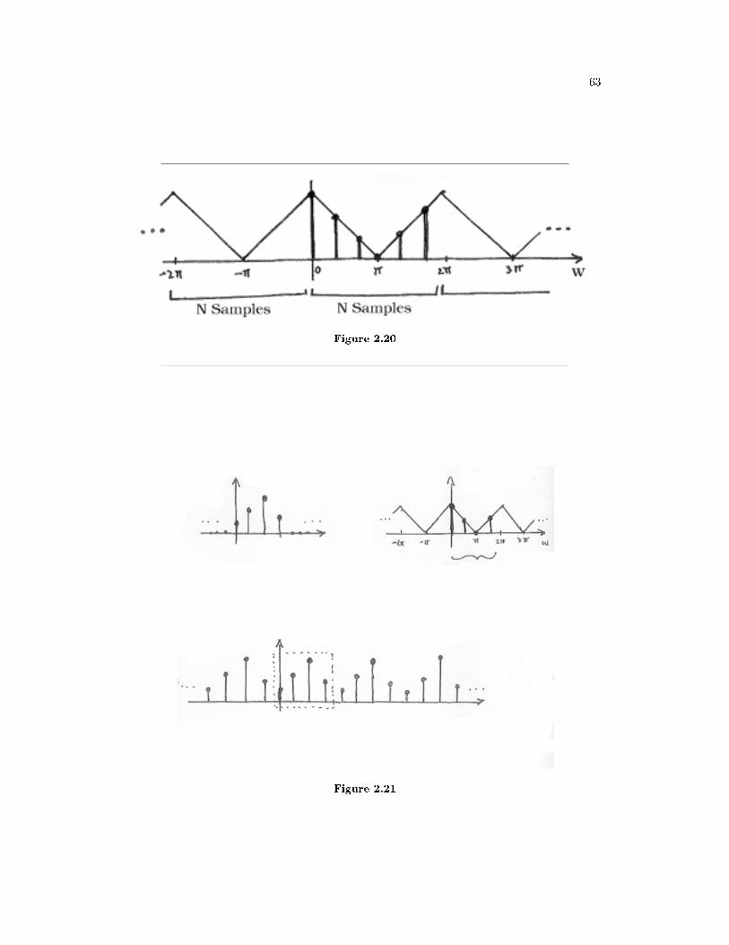
63
Figure 2.20
Figure 2.21

64 CHAPTER 2. SAMPLING AND FREQUENCY ANALYSIS
Figure 2.22
2.7.4 A Sampling PerspectiveThink of sampling the continuous function X (ω), as depicted in Figure 2.22. S (ω) willrepresent the sampling function applied to X (ω) and is illustrated in Figure 2.22 as well.This will result in our discrete-time sequence, X [k].
Recall: Remember the multiplication in the frequency domain is equal to con-volution in the time domain!
2.7.4.1 Inverse DTFT of S(ω)∞∑
k=−∞
(δ
(ω − 2πk
N
))(2.32)

65
Figure 2.23
Given the above equation, we can take the DTFT and get the following equation:N
∞∑m=−∞
(δ [n−mN ]) ≡ S [n] (2.33)
Exercise 2.2:Why does Equation 2.33 equal S [n]?So, in the time-domain we have (Figure 2.23):
2.7.5 ConnectionsCombine signals in Figure 2.24 to get signals in Figure 2.25.
2.8 Discrete-Time Processing of CT Signals2.8.1 DT Processing of CT Signals2.8.1.1 Analysis
Yc (Ω) = HLP (Ω) Y (ΩT ) (2.34)where we know that Y (ω) = X (ω) G (ω) and G (ω) is the frequency response of the DTLTI system. Also, remember that
ω ≡ ΩT
So,Yc (Ω) = HLP (Ω) G (ΩT ) X (ΩT ) (2.35)
where Yc (Ω) and HLP (Ω) are CTFTs and G (ΩT ) and X (ΩT ) are DTFTs.

66 CHAPTER 2. SAMPLING AND FREQUENCY ANALYSIS
Figure 2.24
Figure 2.25

67
DSP System
Figure 2.26
Figure 2.27
Recall:
X (ω) =2π
T
∞∑k=−∞
(Xc
(ω − 2πk
T
))OR
X (ΩT ) =2π
T
∞∑k=−∞
(Xc (Ω− kΩs))
Therefore our nal output signal, Yc (Ω), will be:
Yc (Ω) = HLP (Ω) G (ΩT )
(2π
T
∞∑k=−∞
(Xc (Ω− kΩs))
)(2.36)
Now, if Xc (Ω) is bandlimited to [− (Ωs
2
), Ωs
2
] and we use the usual lowpass reconstructionlter in the D/A, Figure 2.27:
Then,Yc (Ω) =
G (ΩT )Xc (Ω) if |Ω| < Ωs
20 otherwise (2.37)

68 CHAPTER 2. SAMPLING AND FREQUENCY ANALYSIS
Figure 2.28
2.8.1.2 SummaryFor bandlimited signals sampled at or above the Nyquist rate, we can relate the input andoutput of the DSP system by:
Yc (Ω) = Geff (Ω) Xc (Ω) (2.38)where
Geff (Ω) =
G (ΩT ) if |Ω| < Ωs
20 otherwise
2.8.1.2.1 NoteGeff (Ω) is LTI if and only if the following two conditions are satised:
1. G (ω) is LTI (in DT).2. Xc (T ) is bandlimited and sampling rate equal to or greater than Nyquist. For exam-
ple, if we had a simple pulse described byXc (t) = u (t− T0)− u (t− T1)
where T1 > T0. If the sampling period T > T1 − T0, then some samples might "miss"the pulse while others might not be "missed." This is what we term time-varyingbehavior.

69
Figure 2.29
Example 2.8:If 2π
T > 2B and ω1 < BT , determine and sketch Yc (Ω) using Figure 2.29.
2.8.2 Application: 60Hz Noise RemovalUnfortunately, in real-world situations electrodes also pick up ambient 60 Hz signals fromlights, computers, etc.. In fact, usually this "60 Hz noise" is much greater in amplitudethan the EKG signal shown in Figure 2.30. Figure 2.31 shows the EKG signal; it is barelynoticeable as it has become overwhelmed by noise.2.8.2.1 DSP Solution2.8.2.2 Sampling Period/RateFirst we must note that |Y (Ω) | is bandlimited to ±60 Hz. Therefore, the minimum rateshould be 120 Hz. In order to get the best results we should set
fs = 240Hz
.Ωs = 2π
(240
rads
)
2.8.2.3 Digital FilterTherefore, we want to design a digital lter that will remove the 60Hz component andpreserve the rest.

70 CHAPTER 2. SAMPLING AND FREQUENCY ANALYSIS
Figure 2.30
Figure 2.31: Our EKG signal, y (t), is overwhelmed by noise.
Figure 2.32

71
Figure 2.33
Figure 2.34
Figure 2.35

72 CHAPTER 2. SAMPLING AND FREQUENCY ANALYSIS
2.9 Short Time Fourier Transform2.9.1 Short Time Fourier TransformThe Fourier transforms (FT, DTFT, DFT, etc.) do not clearly indicate how the frequencycontent of a signal changes over time.
That information is hidden in the phase - it is not revealed by the plot of the magnitudeof the spectrum.
Note: To see how the frequency content of a signal changes over time, we cancut the signal into blocks and compute the spectrum of each block.
To improve the result,1. blocks are overlapping2. each block is multiplied by a window that is tapered at its endpoints.
Several parameters must be chosen:• Block length, R.• The type of window.• Amount of overlap between blocks. (Figure 2.36)• Amount of zero padding, if any.The short-time Fourier transform is dened as
X (ω, m) = (STFT (x (n)) [U+2254]DTFT (x (n−m)w (n)))=
∑∞n=−∞
(x (n−m) w (n) e−(jωn)
)=
∑R−1n=0
(x (n−m)w (n) e−(jωn)
) (2.39)
where w (n) is the window function of length R.1. The STFT of a signal x (n) is a function of two variables: time and frequency.2. The block length is determined by the support of the window function w (n).3. A graphical display of the magnitude of the STFT, |X (ω, m) |, is called the spectro-gram of the signal. It is often used in speech processing.
4. The STFT of a signal is invertible.5. One can choose the block length. A long block length will provide higher frequency
resolution (because the main-lobe of the window function will be narrow). A shortblock length will provide higher time resolution because less averaging across samplesis performed for each STFT value.
6. A narrow-band spectrogram is one computed using a relatively long block lengthR, (long window function).
7. A wide-band spectrogram is one computed using a relatively short block length R,(short window function).

73
STFT: Overlap Parameter
Figure 2.36

74 CHAPTER 2. SAMPLING AND FREQUENCY ANALYSIS
2.9.1.1 Sampled STFTTo numerically evaluate the STFT, we sample the frequency axis ω in N equally spacedsamples from ω = 0 to ω = 2π.
ωk =2π
Nk , 0 ≤ k ≤ N − 1 (2.40)
We then have the discrete STFT,(Xd (k, m) [U+2254]X
(2πN k,m
))=
∑R−1n=0
(x (n−m) w (n) e−(jωn)
)=
∑R−1n=0
(x (n−m) w (n) WN
−(kn))
= DFTN
(x (n−m) w (n) |R−1
n=0 , 0,. . . 0) (2.41)
where 0,. . . 0 is N −R.In this denition, the overlap between adjacent blocks is R − 1. The signal is shifted
along the window one sample at a time. That generates more points than is usually needed,so we also sample the STFT along the time direction. That means we usually evaluate
Xd (k, Lm)
where L is the time-skip. The relation between the time-skip, the number of overlappingsamples, and the block length is
Overlap = R− L
Exercise 2.3:Match each signal to its spectrogram in Figure 2.37.
2.9.1.2 Spectrogram ExampleThe matlab program for producing the gures above (Figure 2.38 and Figure 2.39).
% LOAD DATA
load mtlb;
x = mtlb;
figure(1), clf
plot(0:4000,x)
xlabel('n')
ylabel('x(n)')
% SET PARAMETERS
R = 256; % R: block length
window = hamming(R); % window function of length R
N = 512; % N: frequency discretization
L = 35; % L: time lapse between blocks
fs = 7418; % fs: sampling frequency
overlap = R - L;

75
(a)
(b)
Figure 2.37

76 CHAPTER 2. SAMPLING AND FREQUENCY ANALYSIS
Figure 2.38
Figure 2.39

77
% COMPUTE SPECTROGRAM
[B,f,t] = specgram(x,N,fs,window,overlap);
% MAKE PLOT
figure(2), clf
imagesc(t,f,log10(abs(B)));
colormap('jet')
axis xy
xlabel('time')
ylabel('frequency')
title('SPECTROGRAM, R = 256')
2.9.1.3 Eect of window length RHere is another example to illustrate the frequency/time resolution trade-o (See gures -Figure 2.40, Figure 2.41, and Figure 2.42).2.9.1.4 Eect of L and NA spectrogram is computed with dierent parameters:
L ∈ 1, 10
N ∈ 32, 256
• L = time lapse between blocks.• N = FFT length (Each block is zero-padded to length N .)
In each case, the block length is 30 samples.Exercise 2.4:For each of the four spectrograms in Figure 2.43 can you tell what L and N are?
L and N do not eect the time resolution or the frequency resolution. They only aectthe 'pixelation'.2.9.1.5 Eect of R and LShown below are four spectrograms of the same signal. Each spectrogram is computed usinga dierent set of parameters.
R ∈ 120, 256, 1024
L ∈ 35, 250
where• R = block length• L = time lapse between blocks.

78 CHAPTER 2. SAMPLING AND FREQUENCY ANALYSIS
Narrow-band spectrogram: better frequency resolution
Figure 2.40

79
Wide-band spectrogram: better time resolution
Figure 2.41

80 CHAPTER 2. SAMPLING AND FREQUENCY ANALYSIS
Eect of Window Length R
(a)
(b)
Figure 2.42

81
(a)
(b)
Figure 2.43

82 CHAPTER 2. SAMPLING AND FREQUENCY ANALYSIS
Figure 2.44

83
Figure 2.45
Exercise 2.5:For each of the four spectrograms in Figure 2.44, match the above values of L andR.If you like, you may listen to this signal with the soundsc command; the data is in the
le: stft_data.m. Here (Figure 2.45) is a gure of the signal.
2.10 SpectrogramsWe know how to acquire analog signals for digital processing (pre-ltering34, sampling35,and A/D conversion36) and to compute spectra of discrete-time signals (using the FFTalgorithm37), let's put these various components together to learn how the spectrogramshown in Figure 2.46, which is used to analyze speech38, is calculated. The speech wassampled at a rate of 11.025 kHz and passed through a 16-bit A/D converter.
point of interest: Music compact discs (CDs) encode their signals at a sam-pling rate of 44.1 kHz. We'll learn the rationale for this number later. The 11.025kHz sampling rate for the speech is 1/4 of the CD sampling rate, and was the low-est available sampling rate commensurate with speech signal bandwidths availableon my computer.
Exercise 2.6:Looking at Figure 2.46 the signal lasted a little over 1.2 seconds. How long was thesampled signal (in terms of samples)? What was the datarate during the samplingprocess in bps (bits per second)? Assuming the computer storage is organized interms of bytes (8-bit quantities), how many bytes of computer memory does thespeech consume?
34http://cnx.org/content/m0050/latest/#ve35http://cnx.org/content/m0050/latest/36http://cnx.org/content/m0051/latest/37http://cnx.org/content/m10250/latest/38http://cnx.org/content/m0049/latest/

84 CHAPTER 2. SAMPLING AND FREQUENCY ANALYSIS
speech spectrogram
Time (s)
Fre
qu
en
cy (
Hz)
0 0.2 0.4 0.6 0.8 1 1.20
1000
2000
3000
4000
5000
Ri ce Uni ver si ty
Figure 2.46

85
Spectrogram Hanning vs. Rectangular256
FFT (512)
RectangularWindow
f
HanningWindow
FFT (512)
n
f
Figure 2.47: The top waveform is a segment 1024 samples long taken from the begin-ning of the "Rice University" phrase. Computing Figure 2.46 involved creating frames,here demarked by the vertical lines, that were 256 samples long and nding the spectrumof each. If a rectangular window is applied (corresponding to extracting a frame from thesignal), oscillations appear in the spectrum (middle of bottom row). Applying a Hanningwindow gracefully tapers the signal toward frame edges, thereby yielding a more accuratecomputation of the signal's spectrum at that moment of time.
The resulting discrete-time signal, shown in the bottom of Figure 2.46, clearly changesits character with time. To display these spectral changes, the long signal was sectionedinto frames: comparatively short, contiguous groups of samples. Conceptually, a Fouriertransform of each frame is calculated using the FFT. Each frame is not so long that signi-cant signal variations are retained within a frame, but not so short that we lose the signal'sspectral character.
An important detail emerges when we examine each framed signal (Figure 2.47). At theframe's edges, the signal may change very abruptly, a feature not present in the originalsignal. A transform of such a segment reveals a curious oscillation in the spectrum, anartifact directly related to this sharp amplitude change. A better way to frame signals forspectrograms is to apply a window: Shape the signal values within a frame so that thesignal decays gracefully as it nears the edges. This shaping is accomplished by multiplyingthe framed signal by the sequence w (n). In sectioning the signal, we essentially applieda rectangular window: w (n) = 1, 0 ≤ n ≤ N − 1. A much more graceful window isthe Hanning window; it has the cosine shape w (n) = 1
2
(1− cos
(2πnN
)). As shown inFigure 2.47, this shaping greatly reduces spurious oscillations in each frame's spectrum.Considering the spectrum of the Hanning windowed frame, we nd that the oscillations

86 CHAPTER 2. SAMPLING AND FREQUENCY ANALYSIS
Hanning speech
n
n
Figure 2.48: In comparison with the original speech segment shown in the upper plot,the non-overlapped Hanning windowed version shown below it is very ragged. Clearly,spectral information extracted from the bottom plot could well miss important featurespresent in the original.
resulting from applying the rectangular window obscured a formant (the one located at alittle more than half the Nyquist frequency).
Exercise 2.7:What might be the source of these oscillations? To gain some insight, what is thelength- 2N discrete Fourier transform of a length-N pulse? The pulse emulatesthe rectangular window, and certainly has edges. Compare your answer with thelength- 2N transform of a length- N Hanning window.If you examine the windowed signal sections in sequence to examine windowing's af-
fect on signal amplitude, we see that we have managed to amplitude-modulate the signalwith the periodically repeated window (Figure 2.48). To alleviate this problem, frames areoverlapped (typically by half a frame duration). This solution requires more Fourier trans-form calculations than needed by rectangular windowing, but the spectra are much betterbehaved and spectral changes are much better captured.
Spectrograms, such as shown in the speech spectrogram (Figure 2.46), are sectioned intooverlapping, equal-length frames, with a Hanning window applied to each frame. The spectraof each of these is calculated, and displayed in spectrograms with frequency extendingvertically, window time location running horizontally, and spectral magnitude color-coded.Figure 2.49 illustrates these computations.
Exercise 2.8:Why the specic values of 256 for N and 512 for K? Another issue is how was thelength-512 transform of each length-256 windowed frame computed?
2.11 Filtering with the DFT2.11.1 Introduction
y [n] = x [n] ∗ h [n]=
∑∞k=−∞ (x [k]h [n− k]) (2.42)

87
Hanning windowsL
og
Sp
ectr
al M
ag
nitu
de
f
n
FFT FFT FFT FFT FFT FFT FFT
Figure 2.49: The original speech segment and the sequence of overlapping Hanningwindows applied to it are shown in the upper portion. Frames were 256 samples longand a Hanning window was applied with a half-frame overlap. A length-512 FFT of eachframe was computed, with the magnitude of the rst 257 FFT values displayed vertically,with spectral amplitude values color-coded.
Figure 2.50

88 CHAPTER 2. SAMPLING AND FREQUENCY ANALYSIS
Figure 2.51
Y (ω) = X (ω) H (ω) (2.43)
Assume that H (ω) is specied.
Exercise 2.9:How can we implement X (ω) H (ω) in a computer?
Recall that the DFT treats N -point sequences as if they are periodically extended (Fig-ure 2.51):

89
Figure 2.52
Figure 2.53: The above symbol for the circular convolution is for an N -periodicextension.
2.11.2 Compute IDFT of Y[k]y [n] = 1
N
∑N−1k=0
(Y [k] ej2π k
N n)
= 1N
∑N−1k=0
(X [k]H [k] ej2π k
N n)
= 1N
∑N−1k=0
((∑N−1m=0
(x [m] e−(j2π k
N m)))
H [k] ej2π kN n)
=∑N−1
m=0
(x [m]
(1N
∑N−1k=0
(H [k] ej2π k
N (n−m))))
=∑N−1
m=0 (x [m]h [((n−m))N ])
(2.44)
And the IDFT periodically extends h [n]:h [n−m] = h [((n−m))N ]
This computes as shown in Figure 2.52:
y [n] =N−1∑m=0
(x [m]h [((n−m))N ]) (2.45)
is called circular convolution and is denoted by Figure 2.53.
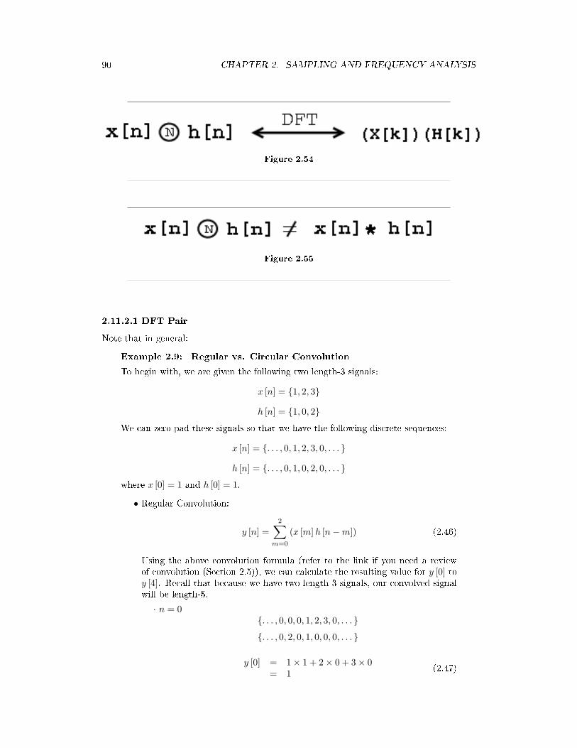
90 CHAPTER 2. SAMPLING AND FREQUENCY ANALYSIS
Figure 2.54
Figure 2.55
2.11.2.1 DFT PairNote that in general:
Example 2.9: Regular vs. Circular ConvolutionTo begin with, we are given the following two length-3 signals:
x [n] = 1, 2, 3
h [n] = 1, 0, 2
We can zero-pad these signals so that we have the following discrete sequences:x [n] = . . . , 0, 1, 2, 3, 0, . . .
h [n] = . . . , 0, 1, 0, 2, 0, . . .
where x [0] = 1 and h [0] = 1.• Regular Convolution:
y [n] =2∑
m=0
(x [m]h [n−m]) (2.46)
Using the above convolution formula (refer to the link if you need a reviewof convolution (Section 2.5)), we can calculate the resulting value for y [0] toy [4]. Recall that because we have two length-3 signals, our convolved signalwill be length-5.· n = 0
. . . , 0, 0, 0, 1, 2, 3, 0, . . .
. . . , 0, 2, 0, 1, 0, 0, 0, . . .
y [0] = 1× 1 + 2× 0 + 3× 0= 1 (2.47)

91
Regular Convolution Result
Figure 2.56: Result is nite duration, not periodic!
· n = 1. . . , 0, 0, 1, 2, 3, 0, . . . . . . , 0, 2, 0, 1, 0, 0, . . .
y [1] = 1× 0 + 2× 1 + 3× 0= 2 (2.48)
· n = 2. . . , 0, 1, 2, 3, 0, . . . . . . , 0, 2, 0, 1, 0, . . .
y [2] = 1× 2 + 2× 0 + 3× 1= 5 (2.49)
· n = 3y [3] = 4 (2.50)
· n = 4y [4] = 6 (2.51)
• Circular Convolution:y [n] =
2∑m=0
(x [m]h [((n−m))N ]) (2.52)
And now with circular convolution our h [n] changes and becomes a periodi-cally extended signal:
h [((n))N ] = . . . , 1, 0, 2, 1, 0, 2, 1, 0, 2, . . . (2.53)
· n = 0. . . , 0, 0, 0, 1, 2, 3, 0, . . . . . . , 1, 2, 0, 1, 2, 0, 1, . . .
y [0] = 1× 1 + 2× 2 + 3× 0= 5 (2.54)

92 CHAPTER 2. SAMPLING AND FREQUENCY ANALYSIS
Circular Convolution Result
Figure 2.57: Result is 3-periodic.
Circular Convolution from Regular
Figure 2.58: The left plot (the circular convolution results) has a "wrap-around" eectdue to periodic extension.
· n = 1. . . , 0, 0, 0, 1, 2, 3, 0, . . .
. . . , 0, 1, 2, 0, 1, 2, 0, . . .
y [1] = 1× 1 + 2× 1 + 3× 2= 8 (2.55)
· n = 2y [2] = 5 (2.56)
· n = 3y [3] = 5 (2.57)
· n = 4y [4] = 8 (2.58)
Figure 2.58 illustrates the relationship between circular convolution and regularconvolution using the previous two gures:

93
Figure 2.59: The sequence from 0 to 4 (the underlined part of the sequence) is theregular convolution result. From this illustration we can see that it is 5-periodic!
2.11.2.2 Regular Convolution from Periodic Convolution1. "Zero-pad" x [n] and h [n] to avoid the overlap (wrap-around) eect. We will zero-pad
the two signals to a length-5 signal (5 being the duration of the regular convolutionresult):
x [n] = 1, 2, 3, 0, 0
h [n] = 1, 0, 2, 0, 0
2. Now take the DFTs of the zero-padded signals:y [n] = 1
N
∑4k=0
(X [k]H [k] ej2π k
5 n)
=∑4
m=0 (x [m]h [((n−m))5])(2.59)
Now we can plot this result (Figure 2.59):General Result: We can compute the regular convolution result of a convolu-tion of an M -point signal x [n] with an N -point signal h [n] by padding each signalwith zeros to obtain two M + N − 1 length sequences and computing the circularconvolution (or equivalently computing the IDFT of H [k]X [k], the product of theDFTs of the zero-padded signals) (Figure 2.60).
2.11.3 DSP System1. Sample nite duration continuous-time input x (t) to get x [n] where n = 0, . . . ,M − 1.2. Zero-pad x [n] and h [n] to length M + N − 1.3. Compute DFTs X [k] and H [k]
4. Compute IDFTs of X [k]H [k]y [n] = y [n]
where n = 0, . . . ,M + N − 1.5. Reconstruct y (t)

94 CHAPTER 2. SAMPLING AND FREQUENCY ANALYSIS
Figure 2.60: Note that the lower two images are simply the top images that have beenzero-padded.
Figure 2.61: The system has a length N impulse response, h [n]

95
Figure 2.62: Fourier Transform (FT) relationship between the two functions.
(a) (b)
Figure 2.63
2.12 Image Restoration Basics2.12.1 Image RestorationIn many applications ( e.g., satellite imaging, medical imaging, astronomical imaging, poor-quality family portraits) the imaging system introduces a slight distortion. Often imagesare slightly blurred and image restoration aims at deblurring the image.
The blurring can usually be modeled as an LSI system with a given PSF h [m,n].The observed image is
g [m,n] = h [m,n] ∗ f [m,n] (2.60)
G (u, v) = H (u, v) F (u, v) (2.61)
F (u, v) =G (u, v)H (u, v)
(2.62)
Example 2.10: Image BlurringAbove we showed the equations for representing the common model for blurringan image. In Figure 2.63 we have an original image and a PSF function that wewish to apply to the image in order to model a basic blurred image.Once we apply the PSF to the original image, we receive our blurred image thatis shown in Figure 2.64:

96 CHAPTER 2. SAMPLING AND FREQUENCY ANALYSIS
Figure 2.64
2.12.1.1 Frequency Domain AnalysisExample 2.10 looks at the original images in its typical form; however, it is often useful tolook at our images and PSF in the frequency domain. In Figure 2.65, we take another lookat the image blurring example above and look at how the images and results would appearin the frequency domain if we applied the fourier transforms.

97
Figure 2.65

98 CHAPTER 2. SAMPLING AND FREQUENCY ANALYSIS
Solutions to Exercises in Chapter 2Solution to Exercise 2.1:
x [n + N ] = ???
Solution to Exercise 2.2:S [n] is N -periodic, so it has the following Fourier Series39:
ck = 1N
∫ N2
−(N2 ) δ [n] e(−j)2π k
N ndn
= 1N
(2.63)
S [n] =∞∑
k=−∞
(e(−j)2π k
N n) (2.64)
where the DTFT of the exponential in the above equation is equal to δ(ω − 2πk
N
).Solution to Exercise 2.3:Solution to Exercise 2.4:Solution to Exercise 2.5:Solution to Exercise 2.6:Number of samples equals 1.2 × 11025 = 13230. The datarate is 11025 × 16 = 176.4 kbps.The storage required would be 26460 bytes.Solution to Exercise 2.7:The oscillations are due to the boxcar window's Fourier transform, which equals the sincfunction.Solution to Exercise 2.8:These numbers are powers-of-two, and the FFT algorithm can be exploited with theselengths. To compute a longer transform than the input signal's duration, we simply zero-pad the signal.Solution to Exercise 2.9:Discretize (sample) X (ω) and H (ω). In order to do this, we should take the DFTs of x [n]and h [n] to get X [k] and X [k]. Then we will compute
y [n] = IDFT (X [k]H [k])
Does y [n] = y [n]?
39http://cnx.org/content/m10496/latest/

Chapter 3
Digital Filtering
3.1 Dierence Equation3.1.1 IntroductionOne of the most important concepts of DSP is to be able to properly represent the in-put/output relationship to a given LTI system. A linear constant-coecient dierenceequation (LCCDE) serves as a way to express just this relationship in a discrete-time sys-tem. Writing the sequence of inputs and outputs, which represent the characteristics of theLTI system, as a dierence equation help in understanding and manipulating a system.
Denition 2: dierence equationAn equation that shows the relationship between consecutive values of a sequenceand the dierences among them. They are often rearranged as a recursive formulaso that a systems output can be computed from the input signal and past outputs.
Example:y [n] + 7y [n− 1] + 2y [n− 2] = x [n]− 4x [n− 1] (3.1)
3.1.2 General Formulas from the Dierence EquationAs stated briey in the denition above, a dierence equation is a very useful tool in describ-ing and calculating the output of the system described by the formula for a given sample n.The key property of the dierence equation is its ability to help easily nd the transform,H (z), of a system. In the following two subsections, we will look at the general form of thedierence equation and the general conversion to a z-transform directly from the dierenceequation.
3.1.2.1 Dierence EquationThe general form of a linear, constant-coecient dierence equation (LCCDE), is shownbelow:
N∑k=0
(aky [n− k]) =M∑
k=0
(bkx [n− k]) (3.2)
99

100 CHAPTER 3. DIGITAL FILTERING
We can also write the general form to easily express a recursive output, which looks likethis:
y [n] = −
(N∑
k=1
(aky [n− k])
)+
M∑k=0
(bkx [n− k]) (3.3)From this equation, note that y [n− k] represents the outputs and x [n− k] represents theinputs. The value of N represents the order of the dierence equation and corresponds tothe memory of the system being represented. Because this equation relies on past values ofthe output, in order to compute a numerical solution, certain past outputs, referred to asthe initial conditions, must be known.3.1.2.2 Conversion to Z-TransformUsing the above formula, Equation 3.2, we can easily generalize the transfer function,H (z), for any dierence equation. Below are the steps taken to convert any dierenceequation into its transfer function, i.e. z-transform. The rst step involves taking theFourier Transform1 of all the terms in Equation 3.2. Then we use the linearity property topull the transform inside the summation and the time-shifting property of the z-transform tochange the time-shifting terms to exponentials. Once this is done, we arrive at the followingequation: a0 = 1.
Y (z) = −
(N∑
k=1
(akY (z) z−k
))+
M∑k=0
(bkX (z) z−k
) (3.4)
H (z) = Y (z)X(z)
=PM
k=0(bkz−k)1+
PNk=1(akz−k)
(3.5)
3.1.2.3 Conversion to Frequency ResponseOnce the z-transform has been calculated from the dierence equation, we can go one stepfurther to dene the frequency response of the system, or lter, that is being representedby the dierence equation.
note: Remember that the reason we are dealing with these formulas is to beable to aid us in lter design. A LCCDE is one of the easiest ways to representFIR lters. By being able to nd the frequency response, we will be able to lookat the basic properties of any lter represented by a simple LCCDE.
Below is the general formula for the frequency response of a z-transform. The conversion issimple a matter of taking the z-transform formula, H (z), and replacing every instance of zwith ejw.
H (w) = H (z) |z,z=ejw
=PM
k=0(bke−(jwk))PNk=0(ake−(jwk))
(3.6)
Once you understand the derivation of this formula, look at the module concerning FilterDesign from the Z-Transform2 for a look into how all of these ideas of the Z-transform(Section 4.2), Dierence Equation, and Pole/Zero Plots (Section 4.4) play a role in lterdesign.
1http://cnx.org/content/m0046/latest/2http://cnx.org/content/m10548/latest/

101
3.1.3 ExampleExample 3.1: Finding Dierence EquationBelow is a basic example showing the opposite of the steps above: given a transferfunction one can easily calculate the systems dierence equation.
H (z) =(z + 1)2(
z − 12
) (z + 3
4
) (3.7)
Given this transfer function of a time-domain lter, we want to nd the dierenceequation. To begin with, expand both polynomials and divide them by the highestorder z.
H (z) = (z+1)(z+1)
(z− 12 )(z+ 3
4 )= z2+2z+1
z2+2z+1− 38
= 1+2z−1+z−2
1+ 14 z−1− 3
8 z−2
(3.8)
From this transfer function, the coecients of the two polynomials will be our akand bk values found in the general dierence equation formula, Equation 3.2. Usingthese coecients and the above form of the transfer function, we can easily writethe dierence equation:
x [n] + 2x [n− 1] + x [n− 2] = y [n] +14y [n− 1]− 3
8y [n− 2] (3.9)
In our nal step, we can rewrite the dierence equation in its more common formshowing the recursive nature of the system.
y [n] = x [n] + 2x [n− 1] + x [n− 2] +−14
y [n− 1] +38y [n− 2] (3.10)
3.1.4 Solving a LCCDEIn order for a linear constant-coecient dierence equation to be useful in analyzing a LTIsystem, we must be able to nd the systems output based upon a known input, x (n), anda set of initial conditions. Two common methods exist for solving a LCCDE: the directmethod and the indirect method, the later being based on the z-transform. Below wewill briey discuss the formulas for solving a LCCDE using each of these methods.
3.1.4.1 Direct MethodThe nal solution to the output based on the direct method is the sum of two parts, expressedin the following equation:
y (n) = yh (n) + yp (n) (3.11)The rst part, yh (n), is referred to as the homogeneous solution and the second part,yh (n), is referred to as particular solution. The following method is very similar to thatused to solve many dierential equations, so if you have taken a dierential calculus courseor used dierential equations before then this should seem very familiar.

102 CHAPTER 3. DIGITAL FILTERING
3.1.4.1.1 Homogeneous SolutionWe begin by assuming that the input is zero, x (n) = 0. Now we simply need to solve thehomogeneous dierence equation:
N∑k=0
(aky [n− k]) = 0 (3.12)
In order to solve this, we will make the assumption that the solution is in the form of anexponential. We will use lambda, λ, to represent our exponential terms. We now have tosolve the following equation:
N∑k=0
(akλn−k
)= 0 (3.13)
We can expand this equation out and factor out all of the lambda terms. This will give usa large polynomial in parenthesis, which is referred to as the characteristic polynomial.The roots of this polynomial will be the key to solving the homogeneous equation. If thereare all distinct roots, then the general solution to the equation will be as follows:
yh (n) = C1(λ1)n + C2(λ2)
n + · · ·+ CN (λN )n (3.14)However, if the characteristic equation contains multiple roots then the above general solu-tion will be slightly dierent. Below we have the modied version for an equation where λ1has K multiple roots:yh (n) = C1(λ1)
n +C1n(λ1)n +C1n
2(λ1)n + · · ·+C1n
K−1(λ1)n +C2(λ2)
n + · · ·+CN (λN )n
(3.15)
3.1.4.1.2 Particular SolutionThe particular solution, yp (n), will be any solution that will solve the general dierenceequation:
N∑k=0
(akyp (n− k)) =M∑
k=0
(bkx (n− k)) (3.16)
In order to solve, our guess for the solution to yp (n) will take on the form of the input,x (n). After guessing at a solution to the above equation involving the particular solution,one only needs to plug the solution into the dierence equation and solve it out.
3.1.4.2 Indirect MethodThe indirect method utilizes the relationship between the dierence equation and z-transform,discussed earlier (Section 3.1.2), to nd a solution. The basic idea is to convert the dier-ence equation into a z-transform, as described above (Section 3.1.2.2), to get the resultingoutput, Y (z). Then by inverse transforming this and using partial-fraction expansion, wecan arrive at the solution.

103
3.2 The Z Transform: Denition3.2.1 Basic Denition of the Z-TransformThe z-transform of a sequence is dened as
X (z) =∞∑
n=−∞
(x [n] z−n
) (3.17)
Sometimes this equation is referred to as the bilateral z-transform. At times the z-transform is dened as
X (z) =∞∑
n=0
(x [n] z−n
) (3.18)
which is known as the unilateral z-transform.There is a close relationship between the z-transform and the Fourier transform of a
discrete time signal, which is dened as
X(ejω)
=∞∑
n=−∞
(x [n] e−(jωn)
) (3.19)
Notice that that when the z−n is replaced with e−(jωn) the z-transform reduces to theFourier Transform. When the Fourier Transform exists, z = ejω , which is to have themagnitude of z equal to unity.
3.2.2 The Complex PlaneIn order to get further insight into the relationship between the Fourier Transform and theZ-Transform it is useful to look at the complex plane or z-plane. Take a look at the complexplane:
The Z-plane is a complex plane with an imaginary and real axis referring to the complex-valued variable z. The position on the complex plane is given by rejω , and the angle fromthe positive, real axis around the plane is denoted by ω. X (z) is dened everywhere on thisplane. X
(ejω) on the other hand is dened only where |z| = 1, which is referred to as the
unit circle. So for example, ω = 1 at z = 1 and ω = π at z = −1. This is useful because, byrepresenting the Fourier transform as the z-transform on the unit circle, the periodicity ofFourier transform is easily seen.
3.2.3 Region of ConvergenceThe region of convergence, known as the ROC, is important to understand because itdenes the region where the z-transform exists. The ROC for a given x [n] , is dened as therange of z for which the z-transform converges. Since the z-transform is a power series, itconverges when x [n] z−n is absolutely summable. Stated dierently,
∞∑n=−∞
(|x [n] z−n|
)< ∞ (3.20)
must be satised for convergence. This is best illustrated by looking at the dierent ROC'sof the z-transforms of αnu [n] and αnu [n− 1].

104 CHAPTER 3. DIGITAL FILTERING
Z-Plane
Figure 3.1
Figure 3.2: x [n] = αnu [n] where α = 0.5.

105
Figure 3.3: ROC for x [n] = αnu [n] where α = 0.5
Example 3.2:For
x [n] = αnu [n] (3.21)
X (z) =∑∞
n=−∞ (x [n] z−n)=
∑∞n=−∞ (αnu [n] z−n)
=∑∞
n=0 (αnz−n)=
∑∞n=0
((αz−1
)n) (3.22)
This sequence is an example of a right-sided exponential sequence because it isnonzero for n ≥ 0. It only converges when |αz−1| < 1. When it converges,
X (z) = 11−αz−1
= zz−α
(3.23)
If |αz−1| ≥ 1, then the series, ∑∞n=0
((αz−1
)n) does not converge. Thus the ROCis the range of values where
|αz−1| < 1 (3.24)or, equivalently,
|z| > |α| (3.25)
Example 3.3:For
x [n] = (− (αn))u [−n− 1] (3.26)

106 CHAPTER 3. DIGITAL FILTERING
Figure 3.4: x [n] = (− (αn)) u [−n− 1] where α = 0.5.
X (z) =∑∞
n=−∞ (x [n] z−n)=
∑∞n=−∞ ((− (αn))u [−n− 1] z−n)
= −(∑−1
n=−∞ (αnz−n))
= −(∑−1
n=−∞
((α−1z
)−n))
= −(∑∞
n=1
((α−1z
)n))= 1−
∑∞n=0
((α−1z
)n)(3.27)
The ROC in this case is the range of values where|α−1z| < 1 (3.28)
or, equivalently,|z| < |α| (3.29)
If the ROC is satised, thenX (z) = 1− 1
1−α−1z
= zz−α
(3.30)
3.3 Table of Common z-TransformsThe table below provides a number of unilateral and bilateral z-transforms (Section 4.2).The table also species the region of convergence3.
3http://cnx.org/content/m10622/latest/

107
Figure 3.5: ROC for x [n] = (− (αn)) u [−n− 1]
note: The notation for z found in the table below may dier from that found inother tables. For example, the basic z-transform of u [n] can be written as eitherof the following two expressions, which are equivalent:
z
z − 1=
11− z−1
(3.31)
Signal Z-Transform ROCδ [n− k] z−k Allz
u [n] zz−1 |z| > 1
− (u [−n− 1]) zz−1 |z| < 1
nu [n] z(z−1)2
|z| > 1
n2u [n] z(z+1)
(z−1)3|z| > 1
n3u [n]z(z2+4z+1)
(z−1)4|z| > 1
(− (αn))u [−n− 1] zz−α |z| < |α|
αnu [n] zz−α |z| > |α|
nαnu [n] αz(z−α)2
|z| > |α|n2αnu [n] αz(z+α)
(z−α)3|z| > |α|Qm
k=1(n−k+1)
αmm! αnu [n] z(z−α)m+1
γncos (αn) u [n] z(z−γcos(α))z2−(2γcos(α))z+γ2 |z| > |γ|
γnsin (αn) u [n] zγsin(α)z2−(2γcos(α))z+γ2 |z| > |γ|

108 CHAPTER 3. DIGITAL FILTERING
3.4 Understanding Pole/Zero Plots on the Z-Plane3.4.1 Introduction to Poles and Zeros of the Z-TransformOnce the Z-transform of a system has been determined, one can use the information con-tained in function's polynomials to graphically represent the function and easily observemany dening characteristics. The Z-transform will have the below structure, based onRational Functions4:
X (z) =P (z)Q (z)
(3.32)
The two polynomials, P (z) and Q (z), allow us to nd the poles and zeros5 of theZ-Transform.
Denition 3: zeros1. The value(s) for z where P (z) = 0.2. The complex frequencies that make the overall gain of the lter transfer functionzero.
Denition 4: poles1. The value(s) for z where Q (z) = 0.2. The complex frequencies that make the overall gain of the lter transfer functioninnite.
Example 3.4:Below is a simple transfer function with the poles and zeros shown below it.
H (z) =z + 1(
z − 12
) (z + 3
4
)The zeros are: −1
The poles are: 12 ,−
(34
)
3.4.2 The Z-PlaneOnce the poles and zeros have been found for a given Z-Transform, they can be plotted ontothe Z-Plane. The Z-plane is a complex plane with an imaginary and real axis referring tothe complex-valued variable z. The position on the complex plane is given by rejθ and theangle from the positive, real axis around the plane is denoted by θ. When mapping polesand zeros onto the plane, poles are denoted by an "x" and zeros by an "o". The below gureshows the Z-Plane, and examples of plotting zeros and poles onto the plane can be found inthe following section.
4http://cnx.org/content/m10593/latest/5http://cnx.org/content/m10112/latest/

109
Z-Plane
Figure 3.6
3.4.3 Examples of Pole/Zero PlotsThis section lists several examples of nding the poles and zeros of a transfer function andthen plotting them onto the Z-Plane.
Example 3.5: Simple Pole/Zero PlotH (z) =
z(z − 1
2
) (z + 3
4
)The zeros are: 0The poles are: 1
2 ,−(
34
)Example 3.6: Complex Pole/Zero Plot
H (z) =(z − j) (z + j)(
z −(
12 −
12j)) (
z −(
12 + 1
2j))
The zeros are: j,−jThe poles are: −1, 1
2 + 12j, 1
2 −12j
MATLAB - If access to MATLAB is readily available, then you can use its functions toeasily create pole/zero plots. Below is a short program that plots the poles and zeros fromthe above example onto the Z-Plane.
% Set up vector for zeros

110 CHAPTER 3. DIGITAL FILTERING
Pole/Zero Plot
Figure 3.7: Using the zeros and poles found from the transfer function, the one zero ismapped to zero and the two poles are placed at 12and − `
34
´
Pole/Zero Plot
Figure 3.8: Using the zeros and poles found from the transfer function, the zeros aremapped to ±j, and the poles are placed at −1, 12
+ 12j and 1
2− 1
2j

111
z = [j ; -j];
% Set up vector for poles
p = [-1 ; .5+.5j ; .5-.5j];
figure(1);
zplane(z,p);
title('Pole/Zero Plot for Complex Pole/Zero Plot Example');
3.4.4 Pole/Zero Plot and Region of ConvergenceThe region of convergence (ROC) for X (z) in the complex Z-plane can be determined fromthe pole/zero plot. Although several regions of convergence may be possible, where each onecorresponds to a dierent impulse response, there are some choices that are more practical.A ROC can be chosen to make the transfer function causal and/or stable depending on thepole/zero plot.Filter Properties from ROC
• If the ROC extends outward from the outermost pole, then the system is causal.• If the ROC includes the unit circle, then the system is stable.
Below is a pole/zero plot with a possible ROC of the Z-transform in the Simple Pole/ZeroPlot (Example 3.5) discussed earlier. The shaded region indicates the ROC chosen for thelter. From this gure, we can see that the lter will be both causal and stable since theabove listed conditions are both met.
Example 3.7:H (z) =
z(z − 1
2
) (z + 3
4
)
3.4.5 Frequency Response and the Z-PlaneThe reason it is helpful to understand and create these pole/zero plots is due to their abilityto help us easily design a lter. Based on the location of the poles and zeros, the magnituderesponse of the lter can be quickly understood. Also, by starting with the pole/zero plot,one can design a lter and obtain its transfer function very easily. Refer to this module6 forinformation on the relationship between the pole/zero plot and the frequency response.
3.5 Filtering in the Frequency DomainBecause we are interested in actual computations rather than analytic calculations, we mustconsider the details of the discrete Fourier transform. To compute the length-N DFT, weassume that the signal has a duration less than or equal to N . Because frequency responses
6http://cnx.org/content/m10548/latest/

112 CHAPTER 3. DIGITAL FILTERING
Region of Convergence for the Pole/Zero Plot
Figure 3.9: The shaded area represents the chosen ROC for the transfer function.
have an explicit frequency-domain specication7 in terms of lter coecients, we don't havea direct handle on which signal has a Fourier transform equaling a given frequency response.Finding this signal is quite easy. First of all, note that the discrete-time Fourier transformof a unit sample equals one for all frequencies. Because of the input and output of linear,shift-invariant systems are related to each other by Y
(ej2πf
)= H
(ej2πf
)X(ej2πf
), a unit-sample input, which has X
(ej2πf
)= 1, results in the output's Fourier transform equaling
the system's transfer function.Exercise 3.1:This statement is a very important result. Derive it yourself.In the time-domain, the output for a unit-sample input is known as the system's unit-
sample response, and is denoted by h (n). Combining the frequency-domain and time-domain interpretations of a linear, shift-invariant system's unit-sample response, we havethat h (n) and the transfer function are Fourier transform pairs in terms of the discrete-timeFourier transform. (
h (n) ↔ H(ej2πf
)) (3.33)Returning to the issue of how to use the DFT to perform ltering, we can analytically
specify the frequency response, and derive the corresponding length-N DFT by samplingthe frequency response.
H (k) = H(e
j2πkN
), k = 0, . . . , N − 1 (3.34)
Computing the inverse DFT yields a length-N signal no matter what the actual durationof the unit-sample response might be. If the unit-sample response has a duration lessthan or equal to N (it's a FIR lter), computing the inverse DFT of the sampled frequencyresponse indeed yields the unit-sample response. If, however, the duration exceeds N , errorsare encountered. The nature of these errors is easily explained by appealing to the Sampling
7http://cnx.org/content/m0510/latest/#dtsinf

113
Theorem. By sampling in the frequency domain, we have the potential for aliasing in thetime domain (sampling in one domain, be it time or frequency, can result in aliasing inthe other) unless we sample fast enough. Here, the duration of the unit-sample responsedetermines the minimal sampling rate that prevents aliasing. For FIR systems theyby denition have nite-duration unit sample responses the number of required DFTsamples equals the unit-sample response's duration: N ≥ q.
Exercise 3.2:Derive the minimal DFT length for a length-q unit-sample response using theSampling Theorem. Because sampling in the frequency domain causes repetitionsof the unit-sample response in the time domain, sketch the time-domain result forvarious choices of the DFT length N .
Exercise 3.3:Express the unit-sample response of a FIR lter in terms of dierence equationcoecients. Note that the corresponding question for IIR lters is far more dicultto answer: Consider the example8.For IIR systems, we cannot use the DFT to nd the system's unit-sample response:
aliasing of the unit-sample response will always occur. Consequently, we can only implementan IIR lter accurately in the time domain with the system's dierence equation. Frequency-domain implementations are restricted to FIR lters.
Another issue arises in frequency-domain ltering that is related to time-domain aliasing,this time when we consider the output. Assume we have an input signal having durationNx that we pass through a FIR lter having a length-q + 1 unit-sample response. What isthe duration of the output signal? The dierence equation for this lter is
y (n) = b0x (n) + · · ·+ bqx (n− q) (3.35)This equation says that the output depends on current and past input values, with the inputvalue q samples previous dening the extent of the lter's memory of past input values. Forexample, the output at index Nx depends on x (Nx) (which equals zero), x (Nx − 1), throughx (Nx − q). Thus, the output returns to zero only after the last input value passes throughthe lter's memory. As the input signal's last value occurs at index Nx−1, the last nonzerooutput value occurs when n − q = Nx − 1 or n = q + Nx − 1. Thus, the output signal'sduration equals q + Nx.
Exercise 3.4:In words, we express this result as "The output's duration equals the input's du-ration plus the lter's duration minus one.". Demonstrate the accuracy of thisstatement.The main theme of this result is that a lter's output extends longer than either its
input or its unit-sample response. Thus, to avoid aliasing when we use DFTs, the dominantfactor is not the duration of input or of the unit-sample response, but of the output. Thus,the number of values at which we must evaluate the frequency response's DFT must be atleast q + Nx and we must compute the same length DFT of the input. To accommodatea shorter signal than DFT length, we simply zero-pad the input: Ensure that for indicesextending beyond the signal's duration that the signal is zero. Frequency-domain ltering,diagrammed in Figure 3.10, is accomplished by storing the lter's frequency response as

114 CHAPTER 3. DIGITAL FILTERING
DFTx(n)
H(k)
IDFTX(k) Y(k) y(n)
Figure 3.10: To lter a signal in the frequency domain, rst compute the DFT of theinput, multiply the result by the sampled frequency response, and nally compute theinverse DFT of the product. The DFT's lengthmust be at least the sum of the input's andunit-sample response's duration minus one. We calculate these discrete Fourier transformsusing the fast Fourier transform algorithm, of course.
the DFT H (k), computing the input's DFT X (k), multiplying them to create the output'sDFT Y (k) = H (k) X (k), and computing the inverse DFT of the result to yield y (n).
Before detailing this procedure, let's clarify why so many new issues arose in trying to de-velop a frequency-domain implementation of linear ltering. The frequency-domain relation-ship9 between a lter's input and output is always true: Y
(ej2πf
)= H
(ej2πf
)X(ej2πf
).This Fourier transforms in this result are discrete-time Fourier transforms; for example,X(ej2πf
)=∑
n
(x (n) e−(j2πfn)
). Unfortunately, using this relationship to perform lter-ing is restricted to the situation when we have analytic formulas for the frequency responseand the input signal. The reason why we had to "invent" the discrete Fourier transform(DFT) has the same origin: The spectrum resulting from the discrete-time Fourier transformdepends on the continuous frequency variable f . That's ne for analytic calculation, butcomputationally we would have to make an uncountably innite number of computations.
note: Did you know that two kinds of innities can be meaningfully dened?A countably innite quantity means that it can be associated with a limitingprocess associated with integers. An uncountably innite quantity cannot be soassociated. The number of rational numbers is countably innite (the numeratorand denominator correspond to locating the rational by row and column; the totalnumber so-located can be counted, voila!); the number of irrational numbers isuncountably innite. Guess which is "bigger?"
The DFT computes the Fourier transform at a nite set of frequencies samples the truespectrum which can lead to aliasing in the time-domain unless we sample sucientlyfast. The sampling interval here is 1
K for a length-K DFT: faster sampling to avoid aliasingthus requires a longer transform calculation. Since the longest signal among the input, unit-sample response and output is the output, it is that signal's duration that determines thetransform length. We simply extend the other two signals with zeros (zero-pad) to computetheir DFTs.
Example 3.8:Suppose we want to average daily stock prices taken over last year to yield arunning weekly average (average over ve trading sessions). The lter we wantis a length-5 averager (as shown in the unit-sample response10), and the input'sduration is 253 (365 calendar days minus weekend days and holidays). The output
8http://cnx.org/content/m10251/latest/#p09http://cnx.org/content/m0510/latest/#equation410http://cnx.org/content/m10251/latest/#g1002

115
Trading Day (1997)
Do
w-J
on
es I
nd
ustr
ial A
ve
rag
e
0 50 100 150 200 2500
1000
2000
3000
4000
5000
6000
7000
8000
Daily AverageWeekly Average
Figure 3.11: The blue line shows the Dow Jones Industrial Average from 1997, and thered one the length-5 boxcar-ltered result that provides a running weekly of this marketindex. Note the "edge" eects in the ltered output.
duration will be 253 + 5 − 1 = 257, and this determines the transform length weneed to use. Because we want to use the FFT, we are restricted to power-of-twotransform lengths. We need to choose any FFT length that exceeds the requiredDFT length. As it turns out, 256 is a power of two (28 = 256), and this length justundershoots our required length. To use frequency domain techniques, we mustuse length-512 fast Fourier transforms.Figure 3.11 shows the input and the ltered output. The MATLAB programs thatcompute the ltered output in the time and frequency domains are
Time Domain
h = [1 1 1 1 1]/5;
y = filter(h,1,[djia zeros(1,4)]);
Frequency Domain
h = [1 1 1 1 1]/5;
DJIA = fft(djia, 512);
H = fft(h, 512);
Y = H.*X;
y = ifft(Y);
note: The filter program has the feature that the length of its outputequals the length of its input. To force it to produce a signal having theproper length, the program zero-pads the input appropriately.
MATLAB's fft function automatically zero-pads its input if the specied trans-form length (its second argument) exceeds the signal's length. The frequency do-main result will have a small imaginary component largest value is 2.2×10⁻¹¹

116 CHAPTER 3. DIGITAL FILTERING
because of the inherent nite precision nature of computer arithmetic. Because ofthe unfortunate mist between signal lengths and favored FFT lengths, the numberof arithmetic operations in the time-domain implementation is far less than thoserequired by the frequency domain version: 514 versus 62,271. If the input sig-nal had been one sample shorter, the frequency-domain computations would havebeen more than a factor of two less (28,696), but far more than in the time-domainimplementation.An interesting signal processing aspect of this example is demonstrated at thebeginning and end of the output. The ramping up and down that occurs can betraced to assuming the input is zero before it begins and after it ends. The lter"sees" these initial and nal values as the dierence equation passes over the input.These artifacts can be handled in two ways: we can just ignore the edge eects orthe data from previous and succeeding years' last and rst week, respectively, canbe placed at the ends.
3.6 Linear-Phase FIR Filters3.6.1 THE AMPLITUDE RESPONSEIf the real and imaginary parts of Hf (ω) are given by
Hf (ω) = Re (ω) + jIm (ω) (3.36)the magnitude and phase are dened as
|Hf (ω) | =√
(Re (ω))2 + (Im (ω))2
p (ω) = arctan(
Im (ω)Re (ω)
)so that
Hf (ω) = |Hf (ω) |ejp(ω) (3.37)With this denition, |Hf (ω) | is never negative and p (ω) is usually discontinuous, but itcan be very helpful to write Hf (ω) as
Hf (ω) = A (ω) ejθ(ω) (3.38)where A (ω) can be positive and negative, and θ (ω) continuous. A (ω) is called the ampli-tude response. Figure 3.12 illustrates the dierence between |Hf (ω) | and A (ω).
A linear-phase phase lter is one for which the continuous phase θ (ω) is linear.Hf (ω) = A (ω) ejθ(ω)
withθ (ω) = (−M) ω + B
We assume in the following that the impulse response h (n) is real-valued.

117
Figure 3.12

118 CHAPTER 3. DIGITAL FILTERING
3.6.2 WHY LINEAR-PHASE?If a discrete-time cosine signal
x1 (n) = cos (ω1n + φ1)
is processed through a discrete-time lter with frequency responseHf (ω) = A (ω) ejθ(ω)
then the output signal is given byy1 (n) = A (ω1) cos (ω1n + φ1 + θ (ω1))
ory1 (n) = A (ω1) cos
(ω1
(n +
θ (ω1)ω1
)+ φ1
)The LTI system has the eect of scaling the cosine signal and delaying it by θ(ω1)
ω1.
Exercise 3.5:When does the system delay cosine signals with dierent frequencies by the sameamount?The function θ(ω)
ω is called the phase delay. A linear phase lter therefore has constantphase delay.3.6.3 WHY LINEAR-PHASE: EXAMPLEConsider a discrete-time lter described by the dierence equationy (n) = −0.1821x (n)+0.7865x (n− 1)−0.6804x (n− 2)+x (n− 3)+0.6804y (n− 1)−0.7865y (n− 2)+0.1821y (n− 3)
(3.39)When ω1 = 0.31π, then the delay is −θ(ω1)
ω1= 2.45. The delay is illustrated in Figure 3.13:
Notice that the delay is fractional the discrete-time samples are not exactly reproducedin the output. The fractional delay can be interpreted in this case as a delay of the underlyingcontinuous-time cosine signal.3.6.4 WHY LINEAR-PHASE: EXAMPLE (2)Consider the same system given on the previous slide, but let us change the frequency ofthe cosine signal.
When ω2 = 0.47π, then the delay is −θ(ω2)ω2
= 0.14.note: For this example, the delay depends on the frequency, because this systemdoes not have linear phase.
3.6.5 WHY LINEAR-PHASE: MOREFrom the previous slides, we see that a lter will delay dierent frequency components of asignal by the same amount if the lter has linear phase (constant phase delay).
In addition, when a narrow band signal (as in AM modulation) goes through a lter, theenvelop will be delayed by the group delay or envelop delay of the lter. The amountby which the envelop is delayed is independent of the carrier frequency only if the lter haslinear phase.
Also, in applications like image processing, lters with non-linear phase can introduceartifacts that are visually annoying.

119
Figure 3.13
3.7 Filter StructuresA realizable lter must require only a nite number of computations per output sample.For linear, causal, time-Invariant lters, this restricts one to rational transfer functions ofthe form
H (z) =b0 + b1z
−1 + · · ·+ bmz−m
1 + a1z−1 + a2z−2 + · · ·+ anz−n
Assuming no pole-zero cancellations, H (z) is FIR if ai = 0 , i > 0 , and IIR otherwise.Filter structures usually implement rational transfer functions as dierence equations.
Whether FIR or IIR, a given transfer function can be implemented with many dierentlter structures. With innite-precision data, coecients, and arithmetic, all lter structuresimplementing the same transfer function produce the same output. However, dierent lterstrucures may produce very dierent errors with quantized data and nite-precision or xed-point arithmetic. The computational expense and memory usage may also dier greatly.Knowledge of dierent lter structures allows DSP engineers to trade o these factors tocreate the best implementation.
3.8 Overview of Digital Filter DesignAdvantages of FIR lters
1. Straight forward conceptually and simple to implement

120 CHAPTER 3. DIGITAL FILTERING
Figure 3.14
2. Can be implemented with fast convolution3. Always stable4. Relatively insensitive to quantization5. Can have linear phase (same time delay of all frequencies)
Advantages of IIR lters
1. Better for approximating analog systems2. For a given magnitude response specication, IIR lters often require much less com-
putation than an equivalent FIR, particularly for narrow transition bandsBoth FIR and IIR lters are very important in applications.Generic Filter Design Procedure
1. Choose a desired response, based on application requirements2. Choose a lter class3. Choose a quality measure4. Solve for the lter in class 2 optimizing criterion in 3

121
3.8.1 Perspective on FIR lteringMost of the time, people do L∞ optimal design, using the Parks-McClellan algorithm (Sec-tion 4.11). This is probably the second most important technique in "classical" signalprocessing (after the Cooley-Tukey (radix-211) FFT).
Most of the time, FIR lters are designed to have linear phase. The most importantadvantage of FIR lters over IIR lters is that they can have exactly linear phase. Thereare advanced design techniques for minimum-phase lters, constrained L2 optimal designs,etc. (see chapter 8 of text). However, if only the magnitude of the response is important,IIR lers usually require much fewer operations and are typically used, so the bulk of FIRlter design work has concentrated on linear phase designs.
3.9 Window Design MethodThe truncate-and-delay design procedure is the simplest and most obvious FIR design pro-cedure.
Exercise 3.6:Is it any Good?
3.9.1 L2 optimization criterionnd h [n] , 0 ≤ n ≤ M−1 , maximizing the energy dierence between the desired responseand the actual response: i.e., nd
minh[n]
∫ π
−π
(|Hd (ω)−H (ω) |)2dω
by Parseval's relationship12minh[n]
∫ π
−π(|Hd (ω)−H (ω) |)2dω
= 2π
∑∞n=−∞
((|hd [n]− h [n] |)2
)= 2π
(∑−1n=−∞
((|hd [n]− h [n] |)2
)+∑M−1
n=0
((|hd [n]− h [n] |)2
)+∑∞
n=M
((|hd [n]− h [n] |)2
))(3.40)
Since = h [n] , n < 0n ≥ M this becomes
minh[n]
∫ π
−π
(|Hd (ω)−H (ω) |)2dω
=
−1∑h=−∞
((|hd [n] |)2
)+
M−1∑n=0
((|h [n]− hd [n] |)2
)+
∞∑n=M
((|hd [n] |)2
)Note: h [n] has no inuence on the rst and last sums.The best we can do is let
h [n] =
hd [n] if 0 ≤ n ≤ M − 10 if else
Thus h [n] = hd [n]w [n],w [n] =
1 if 0 ≤ n (M − 1)
0 if elseis optimal in a least-total-sqaured-error ( L2, or energy) sense!
11http://cnx.org/content/m12016/latest/12http://cnx.org/content/m0047/latest/

122 CHAPTER 3. DIGITAL FILTERING
Exercise 3.7:Why, then, is this design often considered undersirable?For desired spectra with discontinuities, the least-square designs are poor in a minimax
(worst-case, or L∞) error sense.3.9.2 Window Design MethodApply a more gradual truncation to reduce "ringing" (Gibb's Phenomenon13)
,
Note: H (ω) = Hd (ω) ∗W (ω)
The window design procedure (except for the boxcar window) is ad-hoc and not optimalin any usual sense. However, it is very simple, so it is sometimes used for "quick-and-dirty"designs of if the error criterion is itself heurisitic.
3.10 Frequency Sampling Design Method for FIR ltersGiven a desired frequency response, the frequency sampling design method designs a l-ter with a frequency response exactly equal to the desired response at a particular set offrequencies ωk.Procedure
Hd (ωk) =M−1∑n=0
(h (n) e−(jωkn)
), k = [o, 1, . . . , N − 1] (3.41)
Note: Desired Response must incluce linear phase shift (if linear phase is desired)Exercise 3.8:What is Hd (ω) for an ideal lowpass lter, coto at ωc?Note: This set of linear equations can be written in matrix form
Hd (ωk) =M−1∑n=0
(h (n) e−(jωkn)
) (3.42)
Hd (ω0)Hd (ω1)...
Hd (ωN−1)
=
e−(jω00) e−(jω01) . . . e−(jω0(M−1))
e−(jω10) e−(jω11) . . . e−(jω1(M−1))
... ... ... ...e−(jωM−10) e−(jωM−11) . . . e−(jωM−1(M−1))
h (0)h (1)...
h (M − 1)
(3.43)
orHd = Wh
Soh = W−1Hd (3.44)
Note: W is a square matrix for N = M , and invertible as long as ωi 6= ωj +2πl,i 6= j
13http://cnx.org/content/m10092/latest/

123
3.10.1 Important Special CaseWhat if the frequencies are equally spaced between 0 and 2π, i.e. ωk = 2πk
M + αThen
Hd (ωk) =M−1∑n=0
(h (n) e−(j 2πkn
M )e−(jαn))
=M−1∑n=0
((h (n) e−(jαn)
)e−(j 2πkn
M ))
= DFT!
soh (n) e−(jαn) =
1M
M−1∑k=0
(Hd (ωk) e+j 2πnk
M
)or
h [n] =ejαn
M
M−1∑k=0
(Hd [ωk] ej 2πnk
M
)= ejαnIDFT [Hd [ωk]]
3.10.2 Important Special Case 2h [n] symmetric, linear phase, and has real coecients. Since h [n] = h [−1], there are onlyM2 degrees of freedom, and only M
2 linear equations are required.H [ωk] =
∑M−1n=0
(h [n] e−(jωkn)
)=
∑M
2 −1n=0
(h [n]
(e−(jωkn) + e−(jωk(M−n−1))
)) if M even∑M− 32
n=0
(+h [n]
(e−(jωkn) + e−(jωk(M−n−1))
) (h[
M−12
]e−(jωk
M−12 ))) if M odd
=
e−(jωk
M−12 )2
∑M2 −1
n=0
(h [n] cos
(ωk
(M−1
2 − n))) if M even
e−(jωkM−1
2 )2∑M− 3
2n=0
(h [n] cos
(ωk
(M−1
2 − n))
+ h[
M−12
]) if M odd(3.45)
Removing linear phase from both sides yields
A (ωk) =
2∑M
2 −1n=0
(h [n] cos
(ωk
(M−1
2 − n))) if M even
2∑M− 3
2n=0
(h [n] cos
(ωk
(M−1
2 − n))
+ h[
M−12
]) if M oddDue to symmetry of response for real coecients, only M
2 ωk on ω ∈ [0, π) need be specied,with the frequencies −ωk thereby being implicitly dened also. Thus we have M
2 real-valuedsimultaneous linear equations to solve for h [n].3.10.2.1 Special Case 2ah [n] symmetric, odd length, linear phase, real coecients, and ωk equally spaced: ωk =nπkM , 0 ≤ k ≤ M − 1
h [n] = IDFT [Hd (ωk)]= 1
M
∑M−1k=0
(A (ωk) e−(j 2πk
M ) M−12 ej 2πnk
M
)= 1
M
∑M−1k=0
(A (k) ej( 2πk
M (n−M−12 ))
) (3.46)
To yield real coecients, A (ω) mus be symmetricA (ω) = A (−ω) ⇒ A [k] = A [M − k]

124 CHAPTER 3. DIGITAL FILTERING
h [n] = 1M
(A (0) +
∑M−12
k=1
(A [k]
(ej 2πk
M (n−M−12 ) + e−(j2πk(n−M−1
2 )))))
= 1M
(A (0) + 2
∑M−12
k=1
(A [k] cos
(2πkM
(n− M−1
2
))))= 1
M
(A (0) + 2
∑M−12
k=1
(A [k] (−1)kcos
(2πkM
(n + 1
2
)))) (3.47)
Simlar equations exist for even lengths, anti-symmetric, and α = 12 lter forms.
3.10.3 Comments on frequency-sampled designThis method is simple conceptually and very ecient for equally spaced samples, since h [n]can be computed using the IDFT.
H (ω) for a frequency sampled design goes exactly through the sample points, but itmay be very far o from the desired response for ω 6= ωk. This is the main problem withfrequency sampled design.
Possible solution to this problem: specify more frequency samples than degrees of free-dom, and minimize the total error in the frequency response at all of these samples.3.10.4 Extended frequency sample designFor the samples H (ωk) where 0 ≤ k ≤ M − 1 and N > M , nd h [n], where 0 ≤ n ≤ M − 1minimizing ‖ Hd (ωk)−H (ωk) ‖
For ‖ l ‖∞ norm, this becomes a linear programming problem (standard packages avail-ble!)
Here we will consider the ‖ l ‖2 norm.To minimize the ‖ l ‖2 norm; that is,∑N−1
n=0 (|Hd (ωk)−H (ωk) |), we have an overdeter-mined set of linear equations:
e−(jω00) . . . e−(jω0(M−1))
... ... ...e−(jωN−10) . . . e−(jωN−1(M−1))
h =
Hd (ω0)Hd (ω1)...
Hd (ωN−1)
or
Wh = Hd
The minimum error norm solution is well known to be h = (W ∗W )−1W ∗Hd; (W ∗W )−1
W ∗
is well known as the pseudo-inverse matrix.Note: Extended frequency sampled design discourages radical behavior of thefrequency response between samples for suciently closely spaced samples. How-ever, the actual frequency response may no longer pass exactly through any of theHd (ωk).
3.11 Parks-McClellan FIR Filter DesignVery often, the approximation tolerances for a lter are given in terms of the maximumdeviation within bands. For example, we might wish a lowpass lter in a (16-bit) CD playerto have no more than 1
2 -bit deviation in the pass and stop bands.H (ω) =
1− 1
217 ≤ |H (ω) | ≤ 1 + 1217 if |ω| ≤ ωp
1217 ≥ |H (ω) | if ωp ≤ |ω| ≤ π

125
Figure 3.15: The black boxes on the left and right are the passbands, the black boxesin the middle represent the stop band, and the space between the boxes are the transitionbands. Note that overshoots may be allowed in the transition bands.
Typically, we would like to have the shortest-length lter achieving these specications.See Figure 3.15.
Exercise 3.9:Must there be a transition band?
3.11.1 Formal Statement of the L-∞ (Minimax) Design ProblemFor a given lter length (M) and type (odd length, symmetric, linear phase, for example),and a relative error weighting function W (ω), nd the lter coecients minimizing themaximum error
argminh
argmaxω∈F
|E (ω) | = argminh‖ E (ω) ‖∞
whereE (ω) = W (ω) (Hd (ω)−H (ω))
and F is a compact subset of ω ∈ [0, π] ( i.e., all ω in the passbands and stop bands).

126 CHAPTER 3. DIGITAL FILTERING
Note: Typically, we would often rather specify ‖ E (ω) ‖∞ ≤ δ and minimizeover M and h; however, the design techniques minimize δ for a given M . One thenrepeats the design procedure for dierent M until the minimum M satisfying therequirements is found.
We will discuss in detail the design only of odd-length symmetric linear-phase FIR lters.Even-length and anti-symmetric linear phase FIR lters are essentially the same except fora slightly dierent implicit weighting function. For arbitrary phase, exactly optimal designprocedures have only recently been developed (1990).
3.11.2 Outline of L-∞ Filter Design1. Using results from Approximation Theory, simple conditions for determining whether
a given lter is L∞ optimal are found.2. Some ad-hoc iterative methods for nding a lter which satises these condition (and
which is thus optimal) are developed.That is, the L∞ lter design problem is actually solved indirectly.
3.11.3 Conditions for L-∞ Optimality of a Linear-phase FIR FilterAll conditions are based on Chebyshev's "Alternation Theorem," a mathematical fact frompolynomial approximation theory.
3.11.3.1 Alternation TheoremLet F be a compact subset on the real axis x, and let P (x) be and Lth-order polynomial
P (x) =L∑
k=0
(akxk
)Also, let D (x) be a desired function of x that is continuous on F , and W (x) a positive,continuous weighting function on F . Dene the error E (x) on F as
E (x) = W (x) (D (x)− P (x))
and‖ E (x) ‖∞ = argmax
x∈F|E (x) |
A necessary and sucient condition that P (x) is the unique Lth-order polynomial minimiz-ing ‖ E (x) ‖∞ is that E (x) exhibits at least L + 2 "alternations;" that is, there must existat least L+2 values of x, xk ∈ F , k = [0, 1, . . . , L + 1], such that x0 < x1 < · · · < xL+2 andsuch that E (xk) = − (E (xk+1)) = ± (‖ E ‖∞)
Exercise 3.10:What does this have to do with linear-phase lter design?
127
3.11.4 Optimality Conditions for Even-length Symmetric Linear-phase FiltersFor M even,
A (ω) =L∑
n=0
(h (L− n) cos
(ω
(n +
12
)))where L = M
2 −1 Using the trigonometric identity cos (α + β) = cos (α− β)+2cos (α) cos (β)to pull out the ω
2 term and then using the other trig identities (pg 134), it can be shownthat A (ω) can be written as
A (ω) = cos(ω
2
) L∑k=0
(αkcosk (ω)
)Again, this is a polynomial in x = cos (ω), except for a weighting function out in front.
E (ω) = W (ω) (Ad (ω)−A (ω))= W (ω)
(Ad (ω)− cos
(ω2
)P (ω)
)= W (ω) cos
(ω2
)( Ad(ω)
cos(ω2 ) − P (ω)
) (3.48)
which impliesE (x) = W ' (x)
(A'
d (x)− P (x)) (3.49)
whereW ' (x) = W
((cos (x))−1
)cos(
12(cos (x))−1
)and
A'd (x) =
Ad
((cos (x))−1
)cos(
12 (cos (x))−1
)Again, this is a polynomial approximation problem, so the alternation theorem holds. IfE (ω) has at least L + 2 = M
2 + 1 alternations, the even-length symmetric lter is optimalin an L∞ sense.
The prototypical lter design problem:W =
1 if |ω| ≤ ωp
δs
δpif |ωs| ≤ |ω|
See Figure 3.16.3.11.5 L-∞ Optimal Lowpass Filter Design Lemma
1. The maximum possible number of alternations for a lowpass lter is L + 3: Theproof is that the extrema of a polynomial occur only where the derivative is zero:∂∂xP (x) = 0. Since P ′ (x) is an (L− 1)th-order polynomial, it can have at most L− 1zeros. However, the mapping x = cos (ω) implies that ∂
∂ω A (ω) = 0 at ω = 0 andω = π, for two more possible alternation points. Finally, the band edges can also bealternations, for a total of L− 1 + 2 + 2 = L + 3 possible alternations.
2. There must be an alternation at either ω = 0 or ω = π.3. Alternations must occur at ωp and ωs. See Figure 3.16.

128 CHAPTER 3. DIGITAL FILTERING
Figure 3.16

129
4. The lter must be equiripple except at possibly ω = 0 or ω = π. Again see Figure 3.16.Note: The alternation theorem doesn't directly suggest a method for computingthe optimal lter. It simply tells us how to recognize that a lter is optimal, orisn't optimal. What we need is an intelligent way of guessing the optimal ltercoecients.
In matrix form, these L + 2 simultaneous equations become
1 cos (ω0) cos (2ω0) ... cos (Lω0) 1W (ω0)
1 cos (ω1) cos (2ω1) ... cos (Lω1) −1W (ω1)... ... . . . ...
... ...... ... ... . . . ... ...... ... ... .... . . ...
1 cos (ωL+1) cos (2ωL+1) ... cos (LωL+1) ±1W (ωL+1)
h (L)h (L− 1)...
h (1)h (0)
δ
=
Ad (ω0)Ad (ω1).........
Ad (ωL+1)
or
W
(hδ
)= Ad
So, for the given set of L + 2 extremal frequencies, we can solve for h and δ via (h, δ)T =W−1Ad. Using the FFT, we can compute A (ω) of h (n), on a dense set of frequencies. If theold ωk are, in fact the extremal locations of A (ω), then the alternation theorem is satisedand h (n) is optimal. If not, repeat the process with the new extremal locations.
3.11.6 Computational CostO(L3) for the matrix inverse and N log2N for the FFT (N ≥ 32L, typically), per iteration!
This method is expensive computationally due to the matrix inverse.A more ecient variation of this method was developed by Parks and McClellan (1972),
and is based on the Remez exchange algorithm. To understand the Remez exchange algo-rithm, we rst need to understand Lagrange Interpoloation14.
Now A (ω) is an Lth-order polynomial in x = cos (ω), so Lagrange interpolation can beused to exactly compute A (ω) from L + 1 samples of A (ωk), k = [0, 1, 2, ..., L].
Thus, given a set of extremal frequencies and knowing δ, samples of the amplituderesponse A (ω) can be computed directly from the
A (ωk) =(−1)k(+1)
W (ωk)δ + Ad (ωk) (3.50)
without solving for the lter coecients!This leads to computational savings!Note that Equation 3.50 is a set of L + 2 simultaneous equations, which can be solved
for δ to obtain (Rabiner, 1975)
δ =∑L+1
k=0 (γkAd (ωk))∑L+1k=0
((−1)k(+1)γk
W (ωk)
) (3.51)
14http://cnx.org/content/m1/latest/
130 CHAPTER 3. DIGITAL FILTERING
whereγk =
L+1∏i=0i6=k
(1
cos (ωk)− cos (ωi)
)
The result is the Parks-McClellan FIR lter design method, which is simply an applicationof the Remez exchange algorithm to the lter design problem. See Figure 3.17.
The cost per iteration is O(16L2
), as opposed to O(L3); much more ecient for large
L. Can also interpolate to DFT sample frequencies, take inverse FFT to get correspondinglter coecients, and zeropad and take longer FFT to eciently interpolate.
3.12 FIR Filter Design using MATLAB3.12.1 FIR Filter Design Using MATLAB3.12.1.1 Design by windowingThe MATLAB function fir1() designs conventional lowpass, highpass, bandpass, and band-stop linear-phase FIR lters based on the windowing method. The command
b = fir1(N,Wn)
returns in vector b the impulse response of a lowpass lter of order N. The cut-o fre-quency Wn must be between 0 and 1 with 1 corresponding to the half sampling rate.
The command
b = fir1(N,Wn,'high')
returns the impulse response of a highpass lter of order N with normalized cuto fre-quency Wn.
Similarly, b = fir1(N,Wn,'stop') with Wn a two-element vector designating the stop-band designs a bandstop lter.
Without explicit specication, the Hamming window is employed in the design. Otherwindowing functions can be used by specifying the windowing function as an extra argumentof the function. For example, Blackman window can be used instead by the command b =
fir1(N, Wn, blackman(N)).3.12.1.2 Parks-McClellan FIR lter designThe MATLAB command
b = remez(N,F,A)

131
Figure 3.17: The initial guess of extremal frequencies is usually equally spaced inthe band. Computing δ costs O`L2
´. Using Lagrange interpolation costs O (16LL) ≈O
`16L2
´. Computing h (n) costs O`L3
´, but it is only done once!

132 CHAPTER 3. DIGITAL FILTERING
returns the impulse response of the length N+1 linear phase FIR lter of order N designedby Parks-McClellan algorithm. F is a vector of frequency band edges in ascending orderbetween 0 and 1 with 1 corresponding to the half sampling rate. A is a real vector of thesame size as F which species the desired amplitude of the frequency response of the points(F(k),A(k)) and (F(k+1),A(k+1)) for odd k. For odd k, the bands between F(k+1) andF(k+2) is considered as transition bands.
3.13 MATLAB FIR Filter Design Exercise3.13.1 FIR Filter Design MATLAB Exercise3.13.1.1 Design by windowing
Exercise 3.11:Assuming sampling rate at 48kHz, design an order-40 low-pass lter having cut-ofrequency 10kHz by windowing method. In your design, use Hamming window asthe windowing function.
3.13.1.2 Parks-McClellan Optimal DesignExercise 3.12:Assuming sampling rate at 48kHz, design an order-40 lowpass lter having transi-tion band 10kHz-11kHz using the Parks-McClellan optimal FIR lter design algo-rithm.

133
Solutions to Exercises in Chapter 3Solution to Exercise 3.1:The DTFT of the unit sample equals a constant (equaling 1). Thus, the Fourier transformof the output equals the transfer function.Solution to Exercise 3.2:In sampling a discrete-time signal's Fourier transform L times equally over [0, 2π) to formthe DFT, the corresponding signal equals the periodic repetition of the original signal.(
S (k) ↔∞∑
i=−∞(s (n− iL))
)(3.52)
To avoid aliasing (in the time domain), the transform length must equal or exceed thesignal's duration.Solution to Exercise 3.3:The dierence equation for an FIR lter has the form
y (n) =q∑
m=0
(bmx (n−m)) (3.53)
The unit-sample response equals
h (n) =q∑
m=0
(bmδ (n−m)) (3.54)
which corresponds to the representation described in a problem15 of a length-q boxcar lter.Solution to Exercise 3.4:The unit-sample response's duration is q + 1 and the signal's Nx. Thus the statement iscorrect.Solution to Exercise 3.5:• θ(ω)
ω = constant
• θ (ω) = Kω
• The phase is linear.Solution to Exercise 3.6:Yes; in fact it's optimal! (in a certain sense)Solution to Exercise 3.7: Gibbs PhenomenonSolution to Exercise 3.8:
e−(jω M−12 ) if − ωc ≤ ω ≤ ωc
0 if − π ≤ ω < −ωc|ωc < ω ≤ π
15http://cnx.org/content/m10251/latest/#ex2001

134 CHAPTER 3. DIGITAL FILTERING
Solution to Exercise 3.10:It's the same problem! To show that, consider an odd-length, symmetric linear phase lter.
H (ω) =∑M−1
n=0
(h (n) e−(jωn)
)= e−(jω M−1
2 )(h(
M−12
)+ 2
∑Ln=1
(h(
M−12 − n
)cos (ωn)
)) (3.55)
A (ω) = h (L) + 2L∑
n=1
(h (L− n) cos (ωn)) (3.56)
Where (L .= M−12
).Using trigonometric identities (such as cos (nα) = 2cos ((n− 1) α) cos (α)− cos ((n− 2) α)),we can rewrite A (ω) as
A (ω) = h (L) + 2L∑
n=1
(h (L− n) cos (ωn)) =L∑
k=0
(αkcosk (ω)
)where the αk are related to the h (n) by a linear transformation. Now, let x = cos (ω).This is a one-to-one mapping from x ∈ [−1, 1] onto ω ∈ [0, π]. Thus A (ω) is an Lth-orderpolynomial in x = cos (ω)!
implication: The alternation theorem holds for the L∞ lter design problem,too!
Therefore, to determine whether or not a length-M , odd-length, symmetric linear-phase l-ter is optimal in an L∞ sense, simply count the alternations in E (ω) = W (ω) (Ad (ω)−A (ω))in the pass and stop bands. If there are L + 2 = M+3
2 or more alternations, h (n),0 ≤ n ≤ M − 1 is the optimal lter!Solution to Exercise 3.11:
b = fir1(40,10.0/48.0)
Solution to Exercise 3.12:
b = remez(40,[1 1 0 0],[0 10/48 11/48 1])

135
(a)
(b)
Figure 3.18: (a) A (ω), small M (b) A (ω), large M

136 CHAPTER 3. DIGITAL FILTERING

Chapter 4
Statistical and Adaptive Signal
Processing
4.1 Introduction to Random Signals and ProcessesBefore now, you have probably dealt strictly with the theory behind signals and systems, aswell as look at some the basic characteristics of signals1 and systems2. In doing so you havedeveloped an important foundation; however, most electrical engineers do not get to work inthis type of fantasy world. In many cases the signals of interest are very complex due to therandomness of the world around them, which leaves them noisy and often corrupted. Thisoften causes the information contained in the signal to be hidden and distorted. For thisreason, it is important to understand these random signals and how to recover the necessaryinformation.
4.1.1 Signals: Deterministic vs. StochasticFor this study of signals and systems, we will divide signals into two groups: those that havea xed behavior and those that change randomly. As most of you have probably alreadydealt with the rst type, we will focus on introducing you to random signals. Also, note thatwe will be dealing strictly with discrete-time signals since they are the signals we deal within DSP and most real-world computations, but these same ideas apply to continuous-timesignals.4.1.1.1 Deterministic SignalsMost introductions to signals and systems deal strictly with deterministic signals. Eachvalue of these signals are xed and can be determined by a mathematical expression, rule, ortable. Because of this, future values of any deterministic signal can be calculated from pastvalues. For this reason, these signals are relatively easy to analyze as they do not change,and we can make accurate assumptions about their past and future behavior.4.1.1.2 Stochastic SignalsUnlike deterministic signals, stochastic signals, or random signals, are not so nice.Random signals cannot be characterized by a simple, well-dened mathematical equation
1http://cnx.org/content/m10057/latest/2http://cnx.org/content/m10084/latest/
137

138 CHAPTER 4. STATISTICAL AND ADAPTIVE SIGNAL PROCESSING
Deterministic Signal
Figure 4.1: An example of a deterministic signal, the sine wave.
Random Signal
Figure 4.2: We have taken the above sine wave and added random noise to it to comeup with a noisy, or random, signal. These are the types of signals that we wish to learnhow to deal with so that we can recover the original sine wave.
and their future values cannot be predicted. Rather, we must use probability and statisticsto analyze their behavior. Also, because of their randomness, average values (Section 5.3)from a collection of signals are usually studied rather than analyzing one individual signal.
4.1.2 Random ProcessAs mentioned above, in order to study random signals, we want to look at a collection ofthese signals rather than just one instance of that signal. This collection of signals is calleda random process.
Denition 5: random processA family or ensemble of signals that correspond to every possible outcome of acertain signal measurement. Each signal in this collection is referred to as a real-ization or sample function of the process.
Example:As an example of a random process, let us look at the Random SinusoidalProcess below. We use f [n] = Asin (ωn + φ) to represent the sinusoidwith a given amplitude and phase. Note that the phase and amplitude ofeach sinusoid is based on a random number, thus making this a randomprocess.

139
Random Sinusoidal Process
Figure 4.3: A random sinusoidal process, with the amplitude and phase being randomnumbers.

140 CHAPTER 4. STATISTICAL AND ADAPTIVE SIGNAL PROCESSING
A random process is usually denoted by X (t) or X [n], with x (t) or x [n] used to representan individual signal or waveform from this process.
In many notes and books, you might see the following notation and terms used todescribe dierent types of random processes. For a discrete random process, sometimesjust called a random sequence, t represents time that has a nite number of values. Ift can take on any value of time, we have a continuous random process. Often timesdiscrete and continuous refer to the amplitude of the process, and process or sequence referto the nature of the time variable. For this study, we often just use random process torefer to a general collection of discrete-time signals, as seen above in Figure 4.3.
4.2 Stationary and Nonstationary Random Processes4.2.1 IntroductionFrom the denition of a random process (Section 5.1), we know that all random processesare composed of random variables, each at its own unique point in time. Because of this,random processes have all the properties of random variables, such as mean, correlation,variances, etc.. When dealing with groups of signals or sequences it will be important for usto be able to show whether of not these statistical properties hold true for the entire randomprocess. To do this, the concept of stationary processes has been developed. The generaldenition of a stationary process is:
Denition 6: stationary processa random process where all of its statistical properties do not vary with time
Processes whose statistical properties do change are referred to as nonstationary.Understanding the basic idea of stationarity will help you to be able to follow the more
concrete and mathematical denition to follow. Also, we will look at various levels of sta-tionarity used to describe the various types of stationarity characteristics a random processcan have.4.2.2 Distribution and Density FunctionsIn order to properly dene what it means to be stationary from a mathematical standpoint,one needs to be somewhat familiar with the concepts of distribution and density functions.If you can remember your statistics then feel free to skip this section!
Recall that when dealing with a single random variable, the probability distributionfunction is a simply tool used to identify the probability that our observed random variablewill be less than or equal to a given number. More precisely, let X be our random variable,and let x be our given value; from this we can dene the distribution function as
Fx (x) = Pr [X ≤ x] (4.1)This same idea can be applied to instances where we have multiple random variables aswell. There may be situations where we want to look at the probability of event X and Yboth occurring. For example, below is an example of a second-order joint distributionfunction.
Fx (x, y) = Pr [X ≤ x, Y ≤ y] (4.2)While the distribution function provides us with a full view of our variable or processes
probability, it is not always the most useful for calculations. Often times we will want tolook at its derivative, the probability density function (pdf). We dene the the pdf as
fx (x) =d
dxFx (x) (4.3)

141
fx (x) dx = Pr [x < X ≤ x + dx] (4.4)Equation 4.4 reveals some of the physical signicance of the density function. This equa-tions tells us the probability that our random variable falls within a given interval can beapproximated by fx (x) dx. From the pdf, we can now use our knowledge of integrals toevaluate probabilities from the above approximation. Again we can also dene a jointdensity function which will include multiple random variables just as was done for thedistribution function. The density function is used for a variety of calculations, such asnding the expected value or proving a random variable is stationary, to name a few.
note: The above examples explain the distribution and density functions interms of a single random variable, X. When we are dealing with signals andrandom processes, remember that we will have a set of random variables where adierent random variable will occur at each time instance of the random process,X (tk). In other words, the distribution and density function will also need to takeinto account the choice of time.
4.2.3 StationarityBelow we will now look at a more in depth and mathematical denition of a stationaryprocess. As was mentioned previously, various levels of stationarity exist and we will lookat the most common types.
4.2.3.1 First-Order Stationary ProcessA random process is classied as rst-order stationary if its rst-order probability densityfunction remains equal regardless of any shift in time to its time origin. If we let xt1 representa given value at time t1, then we dene a rst-order stationary as one that satises thefollowing equation:
fx (xt1) = fx (xt1+τ ) (4.5)The physical signicance of this equation is that our density function, fx (xt1), is completelyindependent of t1 and thus any time shift, τ .
The most important result of this statement, and the identifying characteristic of anyrst-order stationary process, is the fact that the mean is a constant, independent of anytime shift. Below we show the results for a random process, X, that is a discrete-time signal,x [n].
X = mx [n]= E [x [n]]= constant (independentofn)
(4.6)
4.2.3.2 Second-Order and Strict-Sense Stationary ProcessA random process is classied as second-order stationary if its second-order probabilitydensity function does not vary over any time shift applied to both values. In other words,for values xt1 and xt2 then we will have the following be equal for an arbitrary time shift τ .
fx (xt1 , xt2) = fx (xt1+τ , xt2+τ ) (4.7)

142 CHAPTER 4. STATISTICAL AND ADAPTIVE SIGNAL PROCESSING
From this equation we see that the absolute time does not aect our functions, rather itonly really depends on the time dierence between the two variables. Looked at anotherway, this equation can be described as
Pr [X (t1) ≤ x1, X (t2) ≤ x2] = Pr [X (t1 + τ) ≤ x1, X (t2 + τ) ≤ x2] (4.8)These random processes are often referred to as strict sense stationary (SSS) when
all of the distribution functions of the process are unchanged regardless of the time shiftapplied to them.
For a second-order stationary process, we need to look at the autocorrelation function(Section 5.5) to see its most important property. Since we have already stated that asecond-order stationary process depends only on the time dierence, then all of these typesof processes have the following property:
Rxx (t, t + τ) = E [X (t + τ)]= Rxx (τ) (4.9)
4.2.3.3 Wide-Sense Stationary ProcessAs you begin to work with random processes, it will become evident that the strict require-ments of a SSS process is more than is often necessary in order to adequately approximateour calculations on random processes. We dene a nal type of stationarity, referred to aswide-sense stationary (WSS), to have slightly more relaxed requirements but ones thatare still enough to provide us with adequate results. In order to be WSS a random processonly needs to meet the following two requirements.
1. X = E [x [n]] = constant
2. E [X (t + τ)] = Rxx (τ)
Note that a second-order (or SSS) stationary process will always be WSS; however, thereverse will not always hold true.
4.3 Random Processes: Mean and VarianceIn order to study the characteristics of a random process (Section 5.1), let us look at someof the basic properties and operations of a random process. Below we will focus on theoperations of the random signals that compose our random processes. We will denote ourrandom process with X and a random variable from a random process or signal by x.4.3.1 Mean ValueFinding the average value of a set of random signals or random variables is probably the mostfundamental concepts we use in evaluating random processes through any sort of statisticalmethod. The mean of a random process is the average of all realizations of that process. Inorder to nd this average, we must look at a random signal over a range of time (possiblevalues) and determine our average from this set of values. The mean, or average, of arandom process, x (t), is given by the following equation:
mx (t) = µx (t)= X= E [X]=
∫∞−∞ xf (x) dx
(4.10)

143
This equation may seem quite cluttered at rst glance, but we want to introduce you to thevarious notations used to represent the mean of a random signal or process. Throughouttexts and other readings, remember that these will all equal the same thing. The symbol,µx (t), and the X with a bar over it are often used as a short-hand to represent an average,so you might see it in certain textbooks. The other important notation used is, E [X], whichrepresents the "expected value of X" or the mathematical expectation. This notation is verycommon and will appear again.
If the random variables, which make up our random process, are discrete or quantizedvalues, such as in a binary process, then the integrals become summations over all thepossible values of the random variable. In this case, our expected value becomes
E [x [n]] =∑
x
(αPr [x [n] = α]) (4.11)
If we have two random signals or variables, their averages can reveal how the two signalsinteract. If the product of the two individual averages of both signals do not equal theaverage of the product of the two signals, then the two signals are said to be linearlyindependent, also referred to as uncorrelated.
In the case where we have a random process in which only one sample can be viewed ata time, then we will often not have all the information available to calculate the mean usingthe density function as shown above. In this case we must estimate the mean through thetime-average mean (Section 4.3.4), discussed later. For elds such as signal processing thatdeal mainly with discrete signals and values, then these are the averages most commonlyused.4.3.1.1 Properties of the Mean• The expected value of a constant, α, is the constant:
E [α] = α (4.12)• Adding a constant, α, to each term increases the expected value by that constant:
E [X + α] = E [X] + α (4.13)• Multiplying the random variable by a constant, α, multiplies the expected value by
that constant.E [αX] = αE [X] (4.14)
• The expected value of the sum of two or more random variables, is the sum of eachindividual expected value.
E [X + Y ] = E [X] + E [Y ] (4.15)
4.3.2 Mean-Square ValueIf we look at the second moment of the term (we now look at x2 in the integral), thenwe will have the mean-square value of our random process. As you would expect, this iswritten as
X2 = E[X2]
=∫∞−∞ x2f (x) dx
(4.16)This equation is also often referred to as the average power of a process or signal.

144 CHAPTER 4. STATISTICAL AND ADAPTIVE SIGNAL PROCESSING
4.3.3 VarianceNow that we have an idea about the average value or values that a random process takes,we are often interested in seeing just how spread out the dierent random values might be.To do this, we look at the variance which is a measure of this spread. The variance, oftendenoted by σ2, is written as follows:
σ2 = Var (X)= E
[(X − E [X])2
]=
∫∞−∞
(x−X
)2f (x) dx
(4.17)
Using the rules for the expected value, we can rewrite this formula as the following form,which is commonly seen:
σ2 = X2 −(X)2
= E[X2]− (E [X])2
(4.18)
4.3.3.1 Standard DeviationAnother common statistical tool is the standard deviation. Once you know how to calculatethe variance, the standard deviation is simply the square root of the variance, or σ.4.3.3.2 Properties of Variance• The variance of a constant, α, equals zero:
Var (α) = σ(α)2
= 0(4.19)
• Adding a constant, α, to a random variable does not aect the variance because themean increases by the same value:
Var (X + α) = σ(X + α)2
= σ(X)2(4.20)
• Multiplying the random variable by a constant, α, increases the variance by the squareof the constant:
Var (αX) = σ(αX)2
= α2σ(X)2(4.21)
• The variance of the sum of two random variables only equals the sum of the variancesif the variable are independent.
Var (X + Y ) = σ(X + Y )2
= σ(X)2 + σ(Y )2(4.22)
Otherwise, if the random variable are not independent, then we must also include thecovariance of the product of the variables as follows:
Var (X + Y ) = σ(X)2 + 2Cov (X, Y ) + σ(Y )2 (4.23)

145
4.3.4 Time AveragesIn the case where we can not view the entire ensemble of the random process, we must usetime averages to estimate the values of the mean and variance for the process. Generally,this will only give us acceptable results for independent and ergodic processes, meaningthose processes in which each signal or member of the process seems to have the samestatistical behavior as the entire process. The time averages will also only be taken over anite interval since we will only be able to see a nite part of the sample.4.3.4.1 Estimating the MeanFor the ergodic random process, x (t), we will estimate the mean using the time averagingfunction dened as
X = E [X]= 1
T
∫ T
0X (t) dt
(4.24)However, for most real-world situations we will be dealing with discrete values in our com-putations and signals. We will represent this mean as
X = E [X]= 1
N
∑Nn=1 (X [n])
(4.25)
4.3.4.2 Estimating the VarianceOnce the mean of our random process has been estimated then we can simply use thosevalues in the following variance equation (introduced in one of the above sections)
σx2 = X2 −
(X)2 (4.26)
4.3.5 ExampleLet us now look at how some of the formulas and concepts above apply to a simple example.We will just look at a single, continuous random variable for this example, but the calcula-tions and methods are the same for a random process. For this example, we will considera random variable having the probability density function described below and shown inFigure 4.4.
f (x) =
110 if 10 ≤ x ≤ 20
0 otherwise (4.27)First, we will use Equation 4.10 to solve for the mean value.
X =∫ 20
10x 1
10dx
= 110
(x2
2
)|20x=10
= 110 (200− 50)
= 15
(4.28)
Using Equation 4.16 we can obtain the mean-square value for the above density function.X2 =
∫ 20
10x2 1
10dx
= 110
(x3
3
)|20x=10
= 110
(8000
3 − 10003
)= 233.33
(4.29)

146 CHAPTER 4. STATISTICAL AND ADAPTIVE SIGNAL PROCESSING
Probability Density Function
Figure 4.4: A uniform probability density function.
And nally, let us solve for the variance of this function.σ2 = X2 −
(X)2
= 233.33− 152
= 8.33(4.30)
4.4 Correlation and Covariance of a Random SignalWhen we take the expected value (Section 5.3), or average, of a random process (Sec-tion 4.1.2), we measure several important characteristics about how the process behaves ingeneral. This proves to be a very important observation. However, suppose we have severalrandom processes measuring dierent aspects of a system. The relationship between thesedierent processes will also be an important observation. The covariance and correlationare two important tools in nding these relationships. Below we will go into more detailsas to what these words mean and how these tools are helpful. Note that much of the fol-lowing discussions refer to just random variables, but keep in mind that these variables canrepresent random signals or random processes.4.4.1 CovarianceTo begin with, when dealing with more than one random process, it should be obvious thatit would be nice to be able to have a number that could quickly give us an idea of howsimilar the processes are. To do this, we use the covariance, which is analogous to thevariance of a single variable.
Denition 7: CovarianceA measure of how much the deviations of two or more variables or processes match.
For two processes, X and Y , if they are not closely related then the covariance will be small,and if they are similar then the covariance will be large. Let us clarify this statement bydescribing what we mean by "related" and "similar." Two processes are "closely related" iftheir distribution spreads are almost equal and they are around the same, or a very slightlydierent, mean.

147
Mathematically, covariance is often written as σxy and is dened ascov (X, Y ) = σxy
= E[(
X −X) (
Y − Y)] (4.31)
This can also be reduced and rewritten in the following two forms:σxy = (xy)− (x) (y) (4.32)
σxy =∫ ∞
−∞
∫ ∞
−∞
(X −X
) (Y − Y
)f (x, y) dxdy (4.33)
4.4.1.1 Useful Properties• If X and Y are independent and uncorrelated or one of them has zero mean value,
thenσxy = 0
• If X and Y are orthogonal, thenσxy = − (E [X]E [Y ])
• The covariance is symmetriccov (X, Y ) = cov (Y, X)
• Basic covariance identitycov (X + Y,Z) = cov (X, Z) + cov (Y,Z)
• Covariance of equal variablescov (X, X) = Var (X)
4.4.2 CorrelationFor anyone who has any kind of statistical background, you should be able to see that theidea of dependence/independence among variables and signals plays an important role whendealing with random processes. Because of this, the correlation of two variables providesus with a measure of how the two variables aect one another.
Denition 8: CorrelationA measure of how much one random variable depends upon the other.
This measure of association between the variables will provide us with a clue as to how wellthe value of one variable can be predicted from the value of the other. The correlation isequal to the average of the product of two random variables and is dened as
cor (X, Y ) = E [XY ]=
∫∞−∞
∫∞−∞ xyf (x, y) dxdy
(4.34)

148 CHAPTER 4. STATISTICAL AND ADAPTIVE SIGNAL PROCESSING
(a) (b)
(c)
Figure 4.5: Types of Correlation (a) Positive Correlation (b) Negative Correlation (c)Uncorrelated (No Correlation)
4.4.2.1 Correlation CoecientIt is often useful to express the correlation of random variables with a range of numbers,like a percentage. For a given set of variables, we use the correlation coecient to giveus the linear relationship between our variables. The correlation coecient of two variablesis dened in terms of their covariance and standard deviations (Section 4.3.3.1), denoted byσx, as seen below
ρ =cov (X, Y )
σxσy(4.35)
where we will always have−1 ≤ ρ ≤ 1
This provides us with a quick and easy way to view the correlation between our variables. Ifthere is no relationship between the variables then the correlation coecient will be zero andif there is a perfect positive match it will be one. If there is a perfect inverse relationship,where one set of variables increases while the other decreases, then the correlation coecientwill be negative one. This type of correlation is often referred to more specically as thePearson's Correlation Coecient,or Pearson's Product Moment Correlation.
note: So far we have dealt with correlation simply as a number relating therelationship between any two variables. However, since our goal will be to relaterandom processes to each other, which deals with signals as a function of time,we will want to continue this study by looking at correlation functions (Sec-tion 5.5).

149
4.4.3 ExampleNow let us take just a second to look at a simple example that involves calculating thecovariance and correlation of two sets of random numbers. We are given the following datasets:
x = 3, 1, 6, 3, 4
y = 1, 5, 3, 4, 3
To begin with, for the covariance we will need to nd the expected value (Section 5.3), ormean, of x and y.
x =15
(3 + 1 + 6 + 3 + 4) = 3.4
y =15
(1 + 5 + 3 + 4 + 3) = 3.2
xy =15
(3 + 5 + 18 + 12 + 12) = 10
Next we will solve for the standard deviations of our two sets using the formula below (fora review click here (Section 4.3.3)).
σ =√
E[(X − E [X])2
]σx =
√15
(0.16 + 5.76 + 6.76 + 0.16 + 0.36) = 1.625
σy =
√16
(4.84 + 3.24 + 0.04 + 0.64 + 0.04) = 1.327
Now we can nally calculate the covariance using one of the two formulas found above.Since we calculated the three means, we will use that formula (Equation 4.32) since it willbe much simpler.
σxy = 10− 3.4× 3.2 = −0.88
And for our last calculation, we will solve for the correlation coecient, ρ.ρ =
−0.881.625× 1.327
= −0.408
4.4.3.1 Matlab Code for ExampleThe above example can be easily calculated using Matlab. Below I have included the codeto nd all of the values above.
x = [3 1 6 3 4];
y = [1 5 3 4 3];
mx = mean(x)
my = mean(y)
mxy = mean(x.*y)
% Standard Dev. from built-in Matlab Functions

150 CHAPTER 4. STATISTICAL AND ADAPTIVE SIGNAL PROCESSING
std(x,1)
std(y,1)
% Standard Dev. from Equation Above (same result as std(?,1))
sqrt( 1/5 * sum((x-mx).2))
sqrt( 1/5 * sum((y-my).2))
cov(x,y,1)
corrcoef(x,y)
4.5 Autocorrelation of Random ProcessesBefore diving into a more complex statistical analysis of random signals and processes (Sec-tion 5.1), let us quickly review the idea of correlation (Section 5.4). Recall that the correla-tion of two signals or variables is the expected value of the product of those two variables.Since our focus will be to discover more about a random process, a collection of randomsignals, then imagine us dealing with two samples of a random process, where each sampleis taken at a dierent point in time. Also recall that the key property of these randomprocesses is that they are now functions of time; imagine them as a collection of signals.The expected value (Section 5.3) of the product of these two variables (or samples) will nowdepend on how quickly they change in regards to time. For example, if the two variablesare taken from almost the same time period, then we should expect them to have a highcorrelation. We will now look at a correlation function that relates a pair of random vari-ables from the same process to the time separations between them, where the argument tothis correlation function will be the time dierence. For the correlation of signals from twodierent random process, look at the crosscorrelation function (Section 5.6).4.5.1 Autocorrelation FunctionThe rst of these correlation functions we will discuss is the autocorrelation, where eachof the random variables we will deal with come from the same random process.
Denition 9: Autocorrelationthe expected value of the product of a random variable or signal realization witha time-shifted version of itself
With a simple calculation and analysis of the autocorrelation function, we can discover afew important characteristics about our random process. These include:
1. How quickly our random signal or processes changes with respect to the time function2. Whether our process has a periodic component and what the expected frequency might
beAs was mentioned above, the autocorrelation function is simply the expected value of aproduct. Assume we have a pair of random variables from the same process, X1 = X (t1)and X2 = X (t2), then the autocorrelation is often written as
Rxx (t1, t2) = E [X1X2]=
∫∞−∞
∫∞−∞ x1x2f (x1, x2) dx2dx1
(4.36)

151
The above equation is valid for stationary and nonstationary random processes. For sta-tionary processes (Section 5.2), we can generalize this expression a little further. Given awide-sense stationary processes, it can be proven that the expected values from our ran-dom process will be independent of the origin of our time function. Therefore, we can saythat our autocorrelation function will depend on the time dierence and not some absolutetime. For this discussion, we will let τ = t2− t1, and thus we generalize our autocorrelationexpression as
Rxx (t, t + τ) = Rxx (τ)= E [X (t) X (t + τ)] (4.37)
for the continuous-time case. In most DSP course we will be more interested in dealingwith real signal sequences, and thus we will want to look at the discrete-time case of theautocorrelation function. The formula below will prove to be more common and useful thanEquation 4.36:
Rxx [n, n + m] =∞∑
n=−∞(x [n]x [n + m]) (4.38)
And again we can generalize the notation for our autocorrelation function asRxx [n, n + m] = Rxx [m]
= E [X [n]X [n + m]] (4.39)
4.5.1.1 Properties of AutocorrelationBelow we will look at several properties of the autocorrelation function that hold for sta-tionary random processes.• Autocorrelation is an even function for τ
Rxx (τ) = Rxx (−τ)
• The mean-square value can be found by evaluating the autocorrelation where τ = 0,which gives us
Rxx (0) = X2
• The autocorrelation function will have its largest value when τ = 0. This value canappear again, for example in a periodic function at the values of the equivalent periodicpoints, but will never be exceeded.
Rxx (0) ≥ |Rxx (τ) |
• If we take the autocorrelation of a period function, then Rxx (τ) will also be periodicwith the same frequency.
4.5.1.2 Estimating the Autocorrleation with Time-AveragingSometimes the whole random process is not available to us. In these cases, we would stilllike to be able to nd out some of the characteristics of the stationary random process,even if we just have part of one sample function. In order to do this we can estimate theautocorrelation from a given interval, 0 to T seconds, of the sample function.
xx (τ) =1
T − τ
∫ T−τ
0
x (t)x (t + τ) dt (4.40)

152 CHAPTER 4. STATISTICAL AND ADAPTIVE SIGNAL PROCESSING
n0
x[n]
Figure 4.6: Gaussian density function. By examination, can easily see that the abovestatement is true - the mean equals zero.
However, a lot of times we will not have sucient information to build a complete continuous-time function of one of our random signals for the above analysis. If this is the case, wecan treat the information we do know about the function as a discrete signal and use thediscrete-time formula for estimating the autocorrelation.
xx [m] =1
N −m
N−m−1∑n=0
(x [n]x [n + m]) (4.41)
4.5.2 ExamplesBelow we will look at a variety of examples that use the autocorrelation function. We willbegin with a simple example dealing with Gaussian White Noise (GWN) and a few basicstatistical properties that will prove very useful in these and future calculations.
Example 4.1:We will let x [n] represent our GWN. For this problem, it is important to rememberthe following fact about the mean of a GWN function:
E [x [n]] = 0
Along with being zero-mean, recall that GWN is always independent. With thesetwo facts, we are now ready to do the short calculations required to nd theautocorrelation.
Rxx [n, n + m] = E [x [n]x [n + m]]
Since the function, x [n], is independent, then we can take the product of theindividual expected values of both functions.
Rxx [n, n + m] = E [x [n]]E [x [n + m]]
153
Now, looking at the above equation we see that we can break it up further into twoconditions: one when m and n are equal and one when they are not equal. Whenthey are equal we can combine the expected values. We are left with the followingpiecewise function to solve:
Rxx [n, n + m] =
E [x [n]]E [x [n + m]] if m 6= 0E[x2 [n]
] if m = 0
We can now solve the two parts of the above equation. The rst equation is easyto solve as we have already stated that the expected value of x [n] will be zero. Forthe second part, you should recall from statistics that the expected value of thesquare of a function is equal to the variance. Thus we get the following results forthe autocorrelation:
Rxx [n, n + m] =
0 if m 6= 0σ2 if m = 0
Or in a more concise way, we can represent the results asRxx [n, n + m] = σ2δ [m]
4.6 Crosscorrelation of Random ProcessesBefore diving into a more complex statistical analysis of random signals and processes (Sec-tion 5.1), let us quickly review the idea of correlation (Section 5.4). Recall that the correla-tion of two signals or variables is the expected value of the product of those two variables.Since our main focus is to discover more about random processes, a collection of randomsignals, we will deal with two random processes in this discussion, where in this case wewill deal with samples from two dierent random processes. We will analyze the expectedvalue (Section 4.3.1) of the product of these two variables and how they correlate to oneanother, where the argument to this correlation function will be the time dierence. For thecorrelation of signals from the same random process, look at the autocorrelation function(Section 5.5).4.6.1 Crosscorrelation FunctionWhen dealing with multiple random processes, it is also important to be able to describethe relationship, if any, between the processes. For example, this may occur if more thanone random signal is applied to a system. In order to do this, we use the crosscorrelationfunction, where the variables are instances from two dierent wide sense stationary randomprocesses.
Denition 10: Crosscorrelationif two processes are wide sense stationary, the expected value of the product ofa random variable from one random process with a time-shifted, random variablefrom a dierent random process
Looking at the generalized formula for the crosscorrelation, we will represent our two randomprocesses by allowing U = U (t) and V = V (t− τ). We will dene the crosscorrelationfunction as
Ruv (t, t− τ) = E [UV ]=
∫∞−∞
∫∞−∞ uvf (u, v) dvdu
(4.42)Just as the case with the autocorrelation function, if our input and output, denoted asU (t) and V (t), are at least jointly wide sense stationary, then the crosscorrelation does not

154 CHAPTER 4. STATISTICAL AND ADAPTIVE SIGNAL PROCESSING
depend on absolute time; it is just a function of the time dierence. This means we cansimplify our writing of the above function as
Ruv (τ) = E [UV ] (4.43)or if we deal with two real signal sequences, x [n] and y [n], then we arrive at a morecommonly seen formula for the discrete crosscorrelation function. See the formula belowand notice the similarities between it and the convolution (Section 2.5) of two signals:
Rxy (n, n−m) = Rxy (m)=
∑∞n=−∞ (x [n] y [n−m]) (4.44)
4.6.1.1 Properties of CrosscorrelationBelow we will look at several properties of the crosscorrelation function that hold for twowide sense stationary (WSS) random processes.• Crosscorrelation is not an even function; however, it does have a unique symmetry
property:Rxy (−τ) = Ryx (τ) (4.45)
• The maximum value of the crosscorrelation is not always when the shift equals zero;however, we can prove the following property revealing to us what value the maximumcannot exceed.
|Rxy (τ) | ≤√
Rxx (0)Ryy (0) (4.46)• When two random processes are statistically independent then we have
Rxy (τ) = Ryx (τ) (4.47)
4.6.2 ExamplesExercise 4.1:Let us begin by looking at a simple example showing the relationship between twosequences. Using Equation 4.44, nd the crosscorrelation of the sequences
x [n] = . . . , 0, 0, 2,−3, 6, 1, 3, 0, 0, . . .
y [n] = . . . , 0, 0, 1,−2, 4, 1,−3, 0, 0, . . .
for each of the following possible time shifts: m = 0, 3,−1.
4.7 Introduction to Adaptive FiltersIn many applications requiring ltering, the necessary frequency response may not be knownbeforehand, or it may vary with time. (Example; suppression of engine harmonics in a carstereo.) In such applications, an adaptive lter which can automatically design itself andwhich can track system variations in time is extremely useful. Adaptive lters are usedextensively in a wide variety of applications, particularly in telecommunications.Outline of adaptive lter material

155
Figure 4.7
1. Wiener Filters - L2 optimal (FIR) lter design in a statistical context2. LMS algorithm - simplest and by-far-the-most-commonly-used adaptive lter algo-
rithm3. Stability and performance of the LMS algorithm - When and how well it works4. Applications of adaptive lters - Overview of important applications5. Introduction to advanced adaptive lter algorithms - Techniques for special
situations or faster convergence
4.8 Discrete-Time, Causal Wiener FilterStochastic L2 optimal (least squares) FIR lter design problem: Given a wide-sense sta-tionary (WSS) input signal xk and desired signal dk (WSS ⇔ E [yk] = E [yk+d], ryz (l) =E [ykzk+l], ryy (0) < ∞ , ) The Wiener lter is the linear, time-invariant lter minimizingE[ε2], the variance of the error.
As posed, this problem seems slightly silly, since dk is already available! However, thisidea is useful in a wide cariety of applications.
Example 4.2:active suspension system design
Note: optimal system may change with dierent road conditions ormass in car, so an adaptive system might be desirable.
Example 4.3:System identication (radar, non-destructive testing, adaptive control systems)Exercise 4.2:Usually one desires that the input signal xk be "persistently exciting," which,among other things, implies non-zero energy in all frequency bands. Why is thisdesirable?

156 CHAPTER 4. STATISTICAL AND ADAPTIVE SIGNAL PROCESSING
Figure 4.8
Figure 4.9

157
4.8.1 Determining the optimal length-N causal FIR Weiner lterNote: for convenience, we will analyze only the causal, real-data case; extensionsare straightforward.
yk =M−110∑l=010
(wlxk−l)
argminwl
E[ε210
]= E
[(dk − yk)210
]= E
[(dk −
∑M−110l=010
(wlxk−l))210
]= E
[dk
210]− 210
∑l
= 0M−110 (wlE [dkxk−l]) +
∑M−110l=010
≤ ft(∑M−110
m=010((wlwmE [xk−lxk−m]))
E[ε2]
= rdd (0)− 2M−1∑l=0
(wlrdx (l)) +M−1∑l=0
(M−1∑m=0
(wlwmrxx (l −m))
)where
rdd (0) = E[dk
2]
rdx (l) = E [dkXk−l]
rxx (l −m) = E [xkxk+l−m]
This can be written in matrix form asE[ε2]
= rdd (0)− 2PWT + WT RW
where
P =
rdx (0)rdx (1)...
rdx (M − 1)
R =
rxx (0) rxx (1) . . . . . . rxx (M − 1)
rxx (1) rxx (0). . . . . . ...... . . . . . . . . . ...... . . . . . . rxx (0) rxx (1)
rxx (M − 1) . . . . . . rxx (1) rxx (0)
To solve for the optimum lter, compute the gradient with respect to the top weights vectorW ∇ .=
∂
∂w0
(ε2)
∂∂w1
(ε2)
...∂
∂wM−1
(ε2)
∇ = − (2P) + 2RW
(recall ddW
(AT W
)= AT , d
dW (WMW) = 2MW for symmetric M) setting the gradientequal to zero ⇒ (
WoptR = P⇒ Wopt = R−1P)
Since R is a correlation matrix, it must be non-negative denite, so this is a minimizer. ForR positive denite, the minimizer is unique.

158 CHAPTER 4. STATISTICAL AND ADAPTIVE SIGNAL PROCESSING
4.9 Practical Issues in Wiener Filter ImplementationThe weiner-lter, Wopt = R−1P, is ideal for many applications. But several issues must beaddressed to use it in practice.
Exercise 4.3:In practice one usually won't know exactly the statistics of xk and dk (i.e. R andP) needed to compute the Weiner lter.How do we surmount this problem?Exercise 4.4:In many applications, the statistics of xk, dk vary slowly with time.How does one develop an adaptive system which tracks these changes over timeto keep the system near optimal at all times?Exercise 4.5:How can ˆrk
xx (l) be computed eciently?Exercise 4.6:how does one choose N?
4.9.1 TradeosLarger N → more accurate estimates of the correlation values → better Wopt. However,larger N leads to slower adaptation.
Note: The success of adaptive systems depends on x, d being roughly stationaryover at least N samples, N > M . That is, all adaptive ltering algorithms requirethat the underlying system varies slowly with respect to the sampling rate andthe lter length (although they can tolerate occasional step discontinuities in theunderlying system).
4.9.2 Computational ConsiderationsAs presented here, an adaptive lter requires computing a matrix inverse at each sample.Actually, since the matrix R is Toeplitz, the linear system of equations can be sovled withO(M2) computations using Levinson's algorithm, where M is the lter length. However,
in many applications this may be too expensive, especially since computing the lter out-put itself requires O (M) computations. There are two main approaches to resolving thecomputation problem
1. Take advantage of the fact that Rk+1 is only slightly changed from Rk to reduce thecomputation to O (M); these algorithms are called Fast Recursive Least Squaredsalgorithms; all methods proposed so far have stability problems and are dangerous touse.
2. Find a dierent approach to solving the optimization problem that doesn't requireexplicit inversion of the correlation matrix.Note: Adaptive algorithms involving the correlation matrix are calledRecursiveleast Squares (RLS) algorithms. Historically, they were developed after the LMSalgorithm, which is the slimplest and most widely used approach O (M). O
(M2)
RLS algorithms are used in applications requiring very fast adaptation.

159
Figure 4.10
4.10 Quadratic Minimization and Gradient Descent4.10.1 Quadratic minimization problemsThe least squares optimal lter design problem is quadratic in the lter coecients:
E[ε2]
= rdd (0)− 2PT W + WT RW
If R is positive denite, the error surface E[ε2](w0, w1, . . . , wM−1) is a unimodal "bowl"
in RN . The problem is to nd the bottom of the bowl. In an adaptive lter context, theshape and bottom of the bowl may drift slowly with time; hopefully slow enough that theadaptive algorithm can track it.
For a quadratic error surface, the bottom of the bowl can be found in one step by com-puting R−1P. Most modern nonlinear optimization methods (which are used, for example,to solve the LP optimal IIR lter design problem!) locally approximate a nonlinear func-tion with a second-order (quadratic) Taylor series approximation and step to the bottom ofthis quadratic approximation on each iteration. However, an older and simpler appraoch tononlinear optimaztion exists, based on gradient descent. The idea is to iteratively ndthe minimizer by computing the gradient of the error function: E∇ = ∂
∂wi
(E[ε2]). The
gradient is a vector in RM pointing in the steepest uphill direction on the error surface at agiven point Wi, with ∇ having a magnitude proportional to the slope of the error surfacein this steepest direction.
By updating the coecient vector by taking a step opposite the gradient direction :Wi+1 = Wi − µ∇i, we go (locally) "downhill" in the steepest direction, which seems tobe a sensible way to iteratively solve a nonlinear optimization problem. The performanceobviously depends on µ; if µ is too large, the iterations could bounce back and forth upout of the bowl. However, if µ is too small, it could take many iterations to approach thebottom. We will determine criteria for choosing µ later.
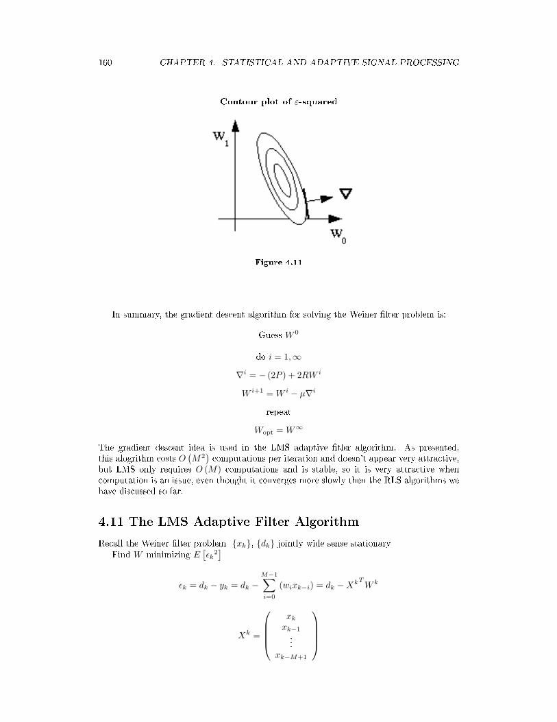
160 CHAPTER 4. STATISTICAL AND ADAPTIVE SIGNAL PROCESSING
Contour plot of ε-squared
Figure 4.11
In summary, the gradient descent algorithm for solving the Weiner lter problem is:Guess W 0
do i = 1,∞
∇i = − (2P ) + 2RW i
W i+1 = W i − µ∇i
repeatWopt = W∞
The gradient descent idea is used in the LMS adaptive tler algorithm. As presented,this alogrithm costs O
(M2) computations per iteration and doesn't appear very attractive,
but LMS only requires O (M) computations and is stable, so it is very attractive whencomputation is an issue, even thought it converges more slowly then the RLS algorithms wehave discussed so far.
4.11 The LMS Adaptive Filter AlgorithmRecall the Weiner lter problem xk, dk jointly wide sense stationary
Find W minimizing E[εk
2]
εk = dk − yk = dk −M−1∑i=0
(wixk−i) = dk −XkTW k
Xk =
xk
xk−1...xk−M+1

161
Figure 4.12
W k =
wk
0
wk1...
wkM−1
The superscript denotes absolute time, and the subscript denotes time or a vector index.
the solution can be found by setting the gradient = 0
∇k = ∂∂W
(E[εk
2])
= E[2εk
(−Xk
)]= E
[−2(dk −XkT
Wk
)Xk]
= −(2E[dkXk
])+(E[XkT
])W
= −2P + 2RW
(4.48)
⇒(Wopt = R−1P
)Alternatively, Wopt can be found iteratively using a gradient descent technique
W k+1 = W k − µ∇k
In practice, we don't know R and P exactly, and in an adaptive context they may be slowlyvarying with time.
To nd the (approximate) Wiener lter, some approximations are necessary. As always,the key is to make the right approximations!
Good idea: Approximate R and P : ⇒ RLS methods, as discussed last time.Better idea: Approximate the gradient!
∇k =∂
∂W
(E[εk
2])
Note that εk2 itself is a very noisy approximation to E
[εk
2]. We can get a noisy approxi-
mation to the gradient by nding the gradient of εk2! Widrow and Ho rst published the
LMS algorithm, based on this clever idea, in 1960.∇k =
∂
∂W
(εk
2)
= 2εk∂
∂W
(dk −W kT
Xk)
= 2εk
(−Xk
)= −
(2εkXk
)

162 CHAPTER 4. STATISTICAL AND ADAPTIVE SIGNAL PROCESSING
This yields the LMS adaptive lter algorithmExample 4.4: The LMS Adaptive Filter Algorithm
1.yk = W kTXk =
∑M−1i=0
(wk
i xk−i
)2.εk = dk − yk
3.W k+1 = W k − µ∇k = W k − µ(−2εkXk
)= W k + 2µεkXk (wk+1
i = wki +
2µεkxk−i)The LMS algorithm is often called a stochastic gradient algorithm, since ∇k is a noisy
gradient. This is by far the most commonly used adaptive ltering algorithm, because1. it was the rst2. it is very simple3. in practice it works well (except that sometimes it converges slowly)4. it requires relatively litle computation5. it updates the tap weights every sample, so it continually adapts the lter6. it tracks slow changes in the signal statistics well
4.11.1 Computational Cost of LMS
To Compute ⇒ yk εk W k+1 = Totalmultiplies M 0 M + 1 2M + 1
adds M − 1 1 M 2M
So the LMS algorithm is O (M) per sample. In fact, it is nicely balanced in that the ltercomputation and the adaptation require the same amount of computation.
Note that the parameter µ plays a very important role in the LMS algorithm. It can alsobe varied with time, but usually a constant µ ("convergence weight facor") is used, chosenafter experimentation for a given application.4.11.1.1 Tradeoslarge µ: fast convergence, fast adaptivity
small µ: accurate W → less misadjustment error, stability
4.12 First Order Convergence Analysis of the LMS Algo-rithm4.12.1 Analysis of the LMS algorithmIt is important to analyze the LMS algorithm to determine under what conditions it isstable, whether or not it converges to the Wiener solution, to determine how quickly itconverges, how much degredation is suered due to the noisy gradient, etc. In particular,we need to know how to choose the parameter µ.

163
4.12.1.1 Mean of Wdoes W k, k →∞ approach the Wiener solution? (since W k is always somewhat random inthe approximate gradient-based LMS algorithm, we ask whether the expected value of thelter coecients converge to the Wiener solution)
E[W k+1
]= W k+1∗
= E[W k + 2µεkXk
]= W k∗ + 2µE
[dkXk
]+ 2µE
[−((
W kTXk)
Xk)]
= W k∗ + 2µP +(−(2µE
[(W kT
Xk)
Xk])) (4.49)
4.12.1.1.1 Patently False AssumptionXk and Xk−i, Xk and dk−i, and dk and dk−i are statistically independent, i 6= 0. Thisassumption is obviously false, since Xk−1 is the same as Xk except for shifting down thevector elements one place and adding one new sample. We make this assumption becauseotherwise it becomes extremely dicult to analyze the LMS algorithm. (First good analysisnot making this assumption: Macchi and Eweda[?] ) Many simulations and much practicalexperience has shown that the results one obtains with analyses based on the patently falseassumption above are quite accurate in most situations
With the independence assumption, W k (which depends only on previous Xk−i, dk−i)is statitically independent of Xk, and we can simplify E
[(W kT
Xk)
Xk]
Now (W kTXk)
Xk is a vector, and
E[(
W kTXk)
Xk]
= E
...(∑M−1i=0
(wk
i xk−i
))xk−j
...
=
...∑M−1
i=0
(E[wk
i xk−ixk−j
])...
=
...∑M−1
i=0
((wk
i
)E [xk−ixk−j ]
)...
=
...∑M−1
i=0
(wk
i∗rxx (i− j)
)...
= RW k∗
(4.50)
where R = E[XkXkT
] is the data correlation matrix.Putting this back into our equation
W k+1 = W k + 2µP +(−(2µRW k
))= (I − 2µR) W k + 2µP
(4.51)

164 CHAPTER 4. STATISTICAL AND ADAPTIVE SIGNAL PROCESSING
Now if W k→∞ converges to a vector of nite magnitude ("convergence in the mean"), whatdoes it converge to?
If W k converges, then as k →∞, W k+1 ≈ W k, andW∞ = (I − 2µR) W∞ + 2µP
2µRW∞ = 2µP
RW∞ = P
orWopt = R−1P
the Wiener solution!So the LMS algorithm, if it converges, gives lter coecients which on average are the
Wiener coecients! This is, of course, a desirable result.4.12.1.2 First-order stabilityBut does W k converge, or under what conditions?
Let's rewrite the analysis in term of V k, the "mean coecient error vector" V k =W k −Wopt, where Wopt is the Wiener lter
W k+1 = W k − 2µRW k + 2µP
W k+1 −Wopt = W k −Wopt +(−(2µRW k
))+ 2µRWopt − 2µRWopt + 2µP
V k+1 = V k − 2µRV k + (− (2µRWopt)) + 2µP
Now Wopt = R−1, soV k+1 = V k − 2µRV k +
(−(2µRR−1P
))+ 2µP = (I − 2µR) V k
We wish to know under what conditions V k→∞ → 0?4.12.1.2.1 Linear Algebra FactSince R is positive denite, real, and symmetric, all the eigenvalues are real and positive.Also, we can write R as (Q−1ΛQ
), where Λ is a diagonal matrix with diagonal entries λiequal to the eigenvalues of R, and Q is a unitary matrix with rows equal to the eigenvectorscorresponding to the eigenvalues of R.
Using this fact,V k+1 =
(I − 2µ
(Q−1ΛQ
))V k
multiplying both sides through on the left by Q: we getQV k+1 = (Q− 2µΛQ)V k = (1− 2µΛ) QV k
Let V ' = QV :V 'k+1 = (1− 2µΛ) V 'k
Note that V ' is simply V in a rotated coordinate set in Rm, so convergence of V ' impliesconvergence of V .
Since 1−2µΛ is diagonal, all elements of V ' evolve independently of each other. Conver-gence (stability) bolis down to whether all M of these scalar, rst-order dierence equationsare stable, and thus → 0.
V 'k+1i = (1− 2µλi)V 'k
i , i = [1, 2, . . . ,M ]
165
These equations converge to zero if |1− 2µλi| < 1, or |µλi| < 1 , µ and λi are positive, sowe require µ < 1λi
, so for convergence in the mean of the LMS adaptive lter, we requireµ <
1λmax
(4.52)This is an elegant theoretical result, but in practice, we may not know λmax, it may be time-varying, and we certainly won't want to compute it. However, another useful mathematicalfact comes to the rescue...
tr (R) =M∑i=1
rii =M∑i=1
λi ≥ λmax
Since the eigenvalues are all positive and real.For a correlation matrix, rii = r (0) , i ∈ 1,M . So tr (R) = Mr (0) = ME [xkxk].
We can easily estimate r (0) with O (1) computations/sample, so in practice we might requireµ <
1
M ˆr (0)
as a conservative bound, and perhaps adapt µ accordingly with time.4.12.1.3 Rate of convergenceEach of the modes decays as
(1− 2µλi)k
Good news: The initial rate of convergence is dominated by the fastest mode1−2µλmax. This is not surprising, since a dradient descent method goes "downhill"in the steepest directionBad news: The nal rate of convergence is dominated by the slowest mode1− 2µλmin. For small λmin, it can take a long time for LMS to converge.
Note that the convergence behavior depends on the data (via R). LMS converges relativelyquickly for roughly equal eigenvalues. Unequal eigenvalues slow LMS down a lot.
4.13 Adaptive Equalizationgoal: Design an approximate inverse lter to cancel out as much distortion aspossible.
In principle, WH ≈ z−∆, or W ≈ z−∆
H , so that the overall response of the top path isapproximately δ (n−∆). However, limitations on the form of W (FIR) and the presence ofnoise cause the equalization to be imperfect.4.13.1 Important ApplicationChannel equalization in a digital communication system. If the channel distorts the pulseshape, the matched lter will no longer be matched, intersymbol interference may increase,and the system performance will degrade.
An adaptive lter is often inserted in front of the matched lter to compensate for thechannel. This is, of course, unrealizable, since we do not have access to the originaltransmitted signal, sk.There are two common solutions to this problem:

166 CHAPTER 4. STATISTICAL AND ADAPTIVE SIGNAL PROCESSING
Figure 4.13
Figure 4.14
Figure 4.15

167
Decision-directed equalizer
Figure 4.16
1. Periodically broadcast a known training signal. The adaptation is switched on onlywhen the training signal is being broadcast and thus sk is known.
2. Decision-directed feedback: If the overall system is working well, then the outputsk−∆0 should almost always equal sk−∆0 . We can thus use our received digital com-munication signal as the desired signal, since it has been cleaned of noise (we hope)by the nonlinear threshold device! As long as the error rate in sk is not too high (say< 75%), this method works. Otherwise, dk is so inaccurate that the adaptive lter cannever nd the Wiener solution. This method is widely used in the telephone systemand other digital communication networks.

168 CHAPTER 4. STATISTICAL AND ADAPTIVE SIGNAL PROCESSING
Solutions to Exercises in Chapter 4Solution to Exercise 4.1:
1.For m = 0, we should begin by nding the product sequence s [n] = x [n] y [n]. Doingthis we get the following sequence:
s [n] = . . . , 0, 0, 2, 6, 24, 1,−9, 0, 0, . . .
and so from the sum in our crosscorrelation function we arrive at the answer ofRxy (0) = 22
2.For m = 3, we will approach it the same was we did above; however, we will now shifty [n] to the right. Then we can nd the product sequence s [n] = x [n] y [n− 3], whichyields
s [n] = . . . , 0, 0, 0, 0, 0, 1,−6, 0, 0, . . .
and from the crosscorrelation function we arrive at the answer ofRxy (3) = −6
3.For m = −1, we will again take the same approach; however, we will now shift y [n] tothe left. Then we can nd the product sequence s [n] = x [n] y [n + 1], which yields
s [n] = . . . , 0, 0,−4,−12, 6,−3, 0, 0, 0, . . .
and from the crosscorrelation function we arrive at the answer ofRxy (−1) = −13
Solution to Exercise 4.3:Estimate the statistics
ˆrxx (l) ≈ 1N
N−1∑k=0
(xkxk+l)
ˆrxd (l) ≈ 1N
N−1∑k=0
(dkxk−l)
then solve Wopt = ˆR−1 = P
Solution to Exercise 4.4:Use short-time windowed estiamtes of the correlation functions.
Equation in Question:
(ˆrxx (l))k
=1N
N−1∑m=0
(xk−mxk−m−l)
(ˆrdx (l))k
=1N
N−1∑m=0
(xk−m−ldk−m)
and Woptk ≈
(Rk
)−1
Pk

169
Solution to Exercise 4.5:Recursively!
rkxx (l) = rk−1
xx (l) + xkxk−l − xk−Nxk−N−l
This is critically stable, so people usually do(1− α) rxx
k (l) = αrk−1xx (l) + xkxk−l

170 CHAPTER 4. STATISTICAL AND ADAPTIVE SIGNAL PROCESSING
Glossary
A Autocorrelation1. the expected value of the product
of a random variable or signalrealization with a time-shiftedversion of itself
C Correlation1. A measure of how much one
random variable depends uponthe other.
Covariance1. A measure of how much the
deviations of two or morevariables or processes match.
Crosscorrelation1. if two processes are wide sense
stationary, the expected value ofthe product of a random variablefrom one random process with atime-shifted, random variablefrom a dierent random process
D dierence equation1. An equation that shows the
relationship between consecutivevalues of a sequence and thedierences among them. Theyare often rearranged as arecursive formula so that asystems output can be computedfrom the input signal and pastoutputs.Example:
y [n] + 7y [n− 1] + 2y [n− 2]
=x[n]− 4x [n− 1] (4.1)F FFT
1. (Fast Fourier Transform) Anecient computational
algorithm for computing theDFT3.
P poles1.The value(s) for z where Q (z) = 0.2. The complex frequencies that
make the overall gain of the ltertransfer function innite.
R random process1. A family or ensemble of signals
that correspond to every possibleoutcome of a certain signalmeasurement. Each signal in thiscollection is referred to as arealization or samplefunction of the process.Example:
As an example of a randomprocess, let us look at theRandom Sinusoidal Processbelow. We usef [n] = Asin (ωn + φ) torepresent the sinusoid with agiven amplitude and phase. Notethat the phase and amplitude ofeach sinusoid is based on arandom number, thus makingthis a random process.
S stationary process1. a random process where all of its
statistical properties do not varywith time
Z zeros1.The value(s) for z where P (z) = 0.2. The complex frequencies that
make the overall gain of the ltertransfer function zero.
3http://cnx.org/content/m10249/latest/

171
Index of Keywords and TermsKeywords are listed by the section with that keyword (page numbers are in paren-theses). Keywords do not necessarily appear in the text of the page. They are merelyassociated with that section. Ex. apples, 1.1 (1) Terms are referenced by the pagethey appear on. Ex. apples, 1
A A/D, 3.7(57), 3.8(65), 3.11(86)adaptive, 155, 158Aliasing, 3.3(49)alphabet, 10amplitude response, 4.6(116), 116analog, 3.7(57), 3.8(65), 4.5(111)analog signal, 2.1(3)analog signals, 4.5(111)Applet, 3.3(49)autocorrelation, 5.2(140), 5.5(150),150, 150average, 5.3(142)average power, 143
B bandlimited, 69basis, 2.6(15), 22, 2.8(30), 30basis matrix, 2.8(30), 31bilateral z-transform, 103block diagram, 2.2(4)blur, 3.12(95)
C cascade, 2.2(4)causal, 111characteristic polynomial, 102circular convolution, 3.11(86), 89coecient vector, 2.8(30), 32commutative, 12complement, 2.6(15), 23complex, 4.4(108)complex exponential sequence, 8computational algorithm, 170continuous frequency, 2.10(34), 2.11(36)continuous random process, 140continuous time, 2.9(33), 2.10(34)Continuous-Time Fourier Transform,34convolution, 2.5(11), 12, 3.11(86), 3.12(95)convolution sum, 12
correlation, 147, 147, 5.5(150)correlation coecient, 148correlation functions, 148countably innite, 114covariance, 146, 146Crosscorrelation, 153crosscorrelation function, 153CT, 3.6(55)CTFT, 2.10(34), 2.13(38), 3.8(65)
D D/A, 3.7(57), 3.8(65), 3.11(86)deblurring, 3.12(95), 95decompose, 2.8(30), 30deconvolution, 3.12(95)delayed, 10density function, 5.2(140)design, 4.11(124)deterministic, 5.1(137)deterministic signals, 137DFT, 2.12(36), 2.13(38), 3.7(57), 3.10(83), 3.11(86), 4.5(111)dierence equation, 2.4(10), 11, 99,99, 4.5(111)digital, 3.7(57), 3.8(65), 4.11(124)digital lter, 4.5(111)digital signal, 2.1(3)digital signal processing, 1(1), 3.10(83), 4.5(111)direct method, 101direct sum, 2.6(15), 23discrete fourier transform, 3.7(57), 3.10(83), 3.11(86), 4.5(111)Discrete Fourier Transform (DFT), 59discrete random process, 140discrete time, 2.5(11), 2.9(33), 2.11(36), 4.3(106)discrete time fourier transform,

172 CHAPTER 4. STATISTICAL AND ADAPTIVE SIGNAL PROCESSING
3.7(57)discrete-time, 4.5(111)discrete-time convolution, 11discrete-time ltering, 4.5(111)distribution function, 5.2(140)DSP, 3.10(83), 3.12(95), 4.3(106), 4.5(111), 4.9(121), 4.10(122), 4.11(124), 5.2(140), 5.3(142), 5.5(150)DT, 2.5(11)DTFT, 2.11(36), 2.13(38), 3.7(57), 3.8(65)
E envelop delay, 118ergodic, 145Examples, 3.3(49)exercise, 4.13(132)
F fast fourier transform, 2.13(38)feedback, 2.2(4)FFT, 2.12(36), 2.13(38), 38lter, 4.10(122), 4.11(124)lter structures, 4.7(119)ltering, 4.5(111)lters, 3.11(86), 4.9(121)nite, 21nite dimensional, 2.6(15), 23FIR, 4.9(121), 4.10(122), 4.11(124), 4.12(130), 4.13(132)FIR lter, 4.8(119)rst order stationary, 5.2(140)rst-order stationary, 141fourier series, 2.9(33)fourier transform, 2.9(33), 2.10(34), 2.11(36), 3.8(65), 3.10(83), 3.11(86), 4.2(103), 103, 4.5(111)fourier transforms, 3.6(55)frames, 85frequency, 3.6(55)frequency domain, 2.13(38)FT, 3.6(55), 3.12(95)functional, 4
G gradient descent, 159group delay, 118
H Hanning window, 3.10(83), 85hilbert, 2.7(29), 2.8(30)Hilbert Space, 2.6(15), 27, 29hilbert spaces, 2.7(29), 2.8(30)Hold, 3.5(53)
homogeneous solution, 101I identity matrix, 32
IIR Filter, 4.8(119)Illustrations, 3.3(49)image, 3.12(95)impulse response, 2.5(11)independent, 144indirect method, 101information, 2.1(3)initial conditions, 100inner, 2.7(29)inner product, 2.7(29)inner product space, 29input, 2.2(4)invertible, 2.6(15), 29
J Java, 3.3(49)joint density function, 5.2(140), 141joint distribution function, 140
K key concepts, 1(1)L laplace transform, 2.9(33)
linear, 4.5(111)linear algebra, 2.12(36)linear and time-invariant, 11Linear discrete-time systems, 10linear transformation, 2.6(15), 27linear-phase FIR lters, 4.6(116)linearly dependent, 2.6(15), 20linearly independent, 2.6(15), 20,143live, 49LTI, 11LTI Systems, 3.8(65)
M Matlab, 3.4(53), 4.12(130), 4.13(132)matrix, 2.12(36)matrix representation, 2.6(15), 28mean, 5.3(142), 142mean-square value, 143moment, 143
N narrow-band spectrogram, 72nonstationary, 5.2(140), 140normed linear space, 29nyquist, 3.6(55)
O optimal, 129order, 100orthogonal, 2.6(15), 25, 29

173
orthogonal compliment, 2.6(15), 26orthonormal, 2.6(15), 25, 2.8(30)orthonormal basis, 2.8(30), 30output, 2.2(4)Overview, 3.1(45)
P parallel, 2.2(4)particular solution, 101pdf, 5.2(140)Pearson's Correlation Coecient, 148phase delay, 118pole, 4.4(108)poles, 108power series, 103probability, 5.2(140)probability density function (pdf), 140probability distribution function, 140probability function, 5.2(140)Proof, 3.2(46)
R random, 5.1(137), 5.3(142), 5.5(150)random process, 5.1(137), 138, 138,140, 5.2(140), 5.3(142), 5.5(150)random sequence, 140random signal, 5.1(137), 5.3(142)random signals, 5.1(137), 137, 5.3(142), 5.5(150)realization, 170Reconstruction, 3.2(46), 3.4(53), 3.5(53)Recursive least Squares, 158restoration, 3.12(95)ROC, 4.2(103), 103
S sample function, 170Sampling, 3.1(45), 3.2(46), 3.3(49), 3.4(53), 3.5(53), 3.6(55), 3.7(57)second order stationary, 5.2(140)second-order stationary, 141Shannon, 3.2(46)shift-invariant, 2.4(10), 11, 4.5(111)short time fourier transform, 3.9(72)signal, 2.1(3), 3, 2.2(4)signals, 2.5(11), 2.9(33)signals and systems, 2.5(11)span, 2.6(15), 21spectrogram, 72spectrograms, 3.10(83)SSS, 5.2(140)
stable, 111standard basis, 2.6(15), 28, 2.8(30)stationarity, 5.2(140)stationary, 5.2(140), 5.5(150)stationary process, 140stationary processes, 140stft, 3.9(72)stochastic, 5.1(137)stochastic gradient, 162stochastic signals, 137strict sense stationary, 5.2(140)strict sense stationary (SSS), 142subspace, 2.6(15), 20superposition, 2.4(10)symmetries, 40System, 3.5(53)system theory, 2.2(4)systems, 2.9(33)
T The stagecoach eect, 52time, 3.6(55)time-varying behavior, 68training signal, 167transfer function, 100, 4.5(111), 4.7(119)transform pairs, 4.3(106)transforms, 33twiddle factors, 40
U uncorrelated, 143uncountably innite, 114unilateral, 4.3(106)unilateral z-transform, 103unique, 30unit sample, 9unit-sample response, 112unitary, 2.6(15), 29
V variance, 5.3(142), 144vector, 2.12(36)vectors, 2.6(15), 19
W well-dened, 2.6(15), 23wide sense stationary, 5.2(140)wide-band spectrogram, 72wide-sense stationary (WSS), 142window, 85WSS, 5.2(140)
Z z transform, 2.9(33), 4.3(106)z-plane, 103, 4.4(108)z-transform, 4.2(103), 103, 4.3(106)

174 CHAPTER 4. STATISTICAL AND ADAPTIVE SIGNAL PROCESSING
z-transforms, 106zero, 4.4(108)
zero-pad, 113zeros, 108

![[Digital signal processing] [li tan] [digital signal processing, fundamentals and applications 2nd ed]](https://static.fdocuments.us/doc/165x107/554a4760b4c9055a408b53bc/digital-signal-processing-li-tan-digital-signal-processing-fundamentals-and-applications-2nd-ed.jpg)