Fundamentals of RF and Microwave Power Measurements (Part ... · damentals of RF and Microwave...

Keysight TechnologiesFundamentals of RF and Microwave Power Measurements (Part 1)

Application Note

Introduction to Power, History, Deinitions, International Standards & Traceability

02 | Keysight | Fundamentals of RF and Microwave Power Measurements (Part 1) – Application Note

Fundamentals of RF and Microwave

Power Measurements (Part 1)

For user convenience, Keysight’s Fun-

damentals of RF and Microwave Power

Measurements, application note 64-1,

literature number 5965-6330E, has been

updated and segmented into four tech-

nical subject groupings. The following

abstracts explain how the total ield of power measurement fundamentals is now

presented.

Fundamentals of RF and Microwave Power Measurements (Part 1)

Introduction to Power, History, Deinitions, International Standards, and Traceability AN 1449-1, literature number 5988-9213ENPart 1 introduces the historical basis for power measurements, and provides deinitions for average, peak, and complex modulations. This application note overviews various

sensor technologies needed for the diversity of test signals. It describes the hierarchy of

international power traceability, yielding comparison to national standards at worldwide

national measurement institutes (NMIs) like the U.S. National Institute of Standards and Technology. Finally, the theory and practice of power sensor comparison procedures are

examined with regard to transferring calibration factors and uncertainties. A glossary is

included which serves all four parts.


Power Sensors and Instrumentation AN 1449-1, literature number 5988-9214ENPart 2 presents all the viable sensor technologies required to exploit the wide range of

unknown modulations and signals under test. It starts with explanations of the sensor

technologies, and how they came to be to meet certain measurement needs. Sensor choices range from the venerable thermistor to the innovative thermocouple to more

recent improvements in diode sensors. In particular, clever variations of diode combina-

tions are presented, which achieve ultra-wide dynamic range and square-law detection

for complex modulations. New instrumentation technologies, which are underpinned

with powerful computational processors, achieve new data performance.


Power Measurement Uncertainty per International Guides AN 1449-1, literature number 5988-9215ENPart 3 discusses the all-important theory and practice of expressing measurement

uncertainty, mismatch considerations, signal lowgraphs, ISO 17025, and examples of typical calculations. Considerable detail is shown on the ISO 17025, Guide for the

Expression of Measurement Uncertainties, has become the international standard for

determining operating speciications. Keysight Technologies, Inc. has transitioned from ANSI/NCSL Z540-1-1994 to ISO 17025.


An Overview of Keysight Instrumentation for RF/Microwave Power Measurements AN 1449-1, literature number 5988-9216ENPart 4 overviews various instrumentation for measuring RF and microwave power,

including spectrum analyzers, microwave receivers, network/spectrum analyzers, and the most accurate method, power sensors/meters. It begins with the unknown signal, of arbitrary modulation format, and draws application-oriented comparisons for selection

of the best instrumentation technology and products.

Most of the chapter is devoted to the most accurate method, power meters and sensors.

It includes comprehensive selection guides,frequency coverages, contrasting accuracy

and dynamic performance to pulsed and complex digital modulations. These are

especially crucial now with the advances in wireless communications formats and

their statistical measurement needs.


Table of Contents Introduction . . . . . . . . . . . . . . . . . . . . . . . . . . . . . . . . . . . . . . . . . . . .4The importance of power . . . . . . . . . . . . . . . . . . . . . . . . . . . . . . . . . . . . . . . . . . . . . . . . . . . 5

A brief history of power measurements . . . . . . . . . . . . . . . . . . . . . . . . . . . . . . . . . . . . . . . . 6

A history of peak power measurements. . . . . . . . . . . . . . . . . . . . . . . . . . . . . . . . . . . . . . . . 7

Power Measurement Fundamentals . . . . . . . . . . . . . . . . . . . . . . . . 9Understanding the characteristics of the signal under test . . . . . . . . . . . . . . . . . . . . . . . 9

Units and deinitions . . . . . . . . . . . . . . . . . . . . . . . . . . . . . . . . . . . . . . . . . . . . . . . . . . . . . . 11

IEEE video pulse standards adapted for microwave pulses . . . . . . . . . . . . . . . . . . . . . . . 15

Peak power waveform deinitions. . . . . . . . . . . . . . . . . . . . . . . . . . . . . . . . . . . . . . . . . . . . 17A typical wireless modulation format. . . . . . . . . . . . . . . . . . . . . . . . . . . . . . . . . . . . . . . . . 18

Three technologies for sensing power . . . . . . . . . . . . . . . . . . . . . . . . . . . . . . . . . . . . . . . 18

An overview of power sensors and meters for pulsed and complex modulations . . . . . 19

Key power sensor parameters . . . . . . . . . . . . . . . . . . . . . . . . . . . . . . . . . . . . . . . . . . . . . . 19

Data computation for statistical parameters of power analysis. . . . . . . . . . . . . . . . . . . . 21

The Chain of Power Traceability . . . . . . . . . . . . . . . . . . . . . . . . . . 22The hierarchy of power measurement, national standards and traceability . . . . . . . . . . 22

The theory and practice of sensor calibration. . . . . . . . . . . . . . . . . . . . . . . . . . . . . . . . . . 24

Some measurement considerations for power sensor comparisons . . . . . . . . . . . . . . . . 25

Typical sensor comparison system. . . . . . . . . . . . . . . . . . . . . . . . . . . . . . . . . . . . . . . . . . . 25

Thermistors as power transfer standards . . . . . . . . . . . . . . . . . . . . . . . . . . . . . . . . . . . . . 27Other DC substitution meters. . . . . . . . . . . . . . . . . . . . . . . . . . . . . . . . . . . . . . . . . . . . . . . 27Peak power sensor calibration traceability . . . . . . . . . . . . . . . . . . . . . . . . . . . . . . . . . . . . 28

Network analyzer source system . . . . . . . . . . . . . . . . . . . . . . . . . . . . . . . . . . . . . . . . . . . 29

NIST six-port calibration system . . . . . . . . . . . . . . . . . . . . . . . . . . . . . . . . . . . . . . . . . . . 29

General references . . . . . . . . . . . . . . . . . . . . . . . . . . . . . . . . . . . . . . . . . . . . . . . . . . . . . . . 30

Glossary and List of Symbols . . . . . . . . . . . . . . . . . . . . . . . . . . . . 31


The purpose of the new series of Fundamentals of RF and Microwave Power

Measurements application notes, which were leveraged from former note 64-1, is to:

1. Retain tutorial information about historical and fundamental considerations of RF/microwave power measurements and technology which tend to remain timeless.

2. Provide current information on new meter and sensor technology.

3. Present the latest modern power measurement techniques and test equipment

that represents the current state-of-the-art.

Part 1, Chapter 1 reviews the commercial and technical importance of making power

measurements, equity in trade, the cost of measurement uncertainties, and the need for

two power measurements of the same unit under test will be the same at two locations in

the world. It then presents a brief history of power techniques, and additionally a history

of peak power techniques.

Chapter 2 shows why it is crucial to begin a power measurement task with a clear under-

standing of the characteristics of the signal under test. With the advent of new complex

combinations of modulations in the 1990s and forward, it also presents signal format

considerations that users must evaluate when pondering which sensor technologies to use.

The application note then deines the variety of terminology of units and deinitions of various power measuring terms. It shows how IEEE video pulse standards were adapted

by Keysight for use in microwave pulsed power envelopes. Brief descriptions of modern

wireless formats show how key sensor performance is required to faithfully capture the

system power. Various sensor technologies and instrumentation are previewed from the

complete descriptions in Fundamentals Part 2.

Considerations necessary for capturing and digitizing microwave signals which are used

in modern wireless systems are presented. These often consist of pulsed carriers plus

digital phase modulations, which look like noise, combined on the same signal. When

measured with digital sampling type instrumentation, the powerful micro-processors

can run statistical routines to reveal computed data, oriented to particular customer

requirements.

Chapter 3 presents the matter of basic measurement traceability to national and world

standards. It describes the hierarchy of international traceability, including comparison

processes to national standards at worldwide NMIs such as the U.S. National Institute of Standards and Technology, Boulder, CO.

The application note reviews the theory and practice of sensor calibration processes and

the need for transportable sensor artifacts which can transfer higher-echelon uncertainties

of the NMIs to company primary lab standards. It reviews special procedures needed for

extended calibration processes on pulse-power sensors.

Note: In this application note numerous technical references will be made to the other

published parts of the Fundamentals of RF and Microwave Power Measurements series.

For brevity, we will use the format Fundamentals Part X. This should insure that you

can quickly locate the concept in the other publication. Brief abstracts for the four-part

series are provided on the inside the front cover.

Introduction


The importance of power

The output power level of a system or component is frequently the critical factor in the

design, and ultimately the purchase and performance of almost all radio frequency and

microwave equipment. The irst key factor is the concept of equity in trade. When a cus-

tomer purchases a product with speciied power performance for a negotiated price, the inal production-line test results need to agree with the customer’s incoming inspection data. These shipping, receiving, installation or commissioning phases often occur at

different locations, and sometimes across national borders. The various measurements

must be consistent within acceptable uncertainties.

Secondly, measurement uncertainties cause ambiguities in the realizable performance of a transmitter. For example, a 10-W transmitter costs more than a 5-W transmitter. Twice

the power output means twice the geographical area is covered or 40% more radial

range for a communication system. Yet, if the overall measurement uncertainty of the

inal product test is on the order of ±0.5 dB, the unit actually shipped could have output power as much as 10% lower than the customer expects, with resulting lower operating

margins.

Because signal power level is so important to the overall system performance, it is also

critical when specifying the components that build up the system. Each component of a

signal chain must receive the proper signal level from the previous component and pass

the proper level to the succeeding component. Power is so important that it is frequently

measured twice at each level, once by the vendor and again at the incoming inspection

stations before beginning the next assembly level. It is at the higher operating power

levels where each decibel increase in power level becomes more costly in terms of

complexity of design, expense of active devices, skill in manufacture, dificulty of testing, and degree of reliability.

The increased cost per dB of power level is especially true at microwave frequencies,

where the high-power solid state devices are inherently more costly and the guard-bands

designed into the circuits to avoid maximum device stress are also quite costly. Many

systems are continuously monitored for output power during ordinary operation. This

large number of power measurements and their importance dictates that the measurement

equipment and techniques be accurate, repeatable, traceable, and convenient.

The goal of this application note, and others, is to guide the reader in making those

measurement qualities routine. Because many of the examples cited above used the

term “signal level,” the natural tendency might be to suggest measuring voltage instead

of power. At low frequencies, below about 100 kHz, power is usually calculated from

voltage measurements across an assumed impedance. As the frequency increases, the

impedance has large variations, so power measurements become more popular, and

voltage or current are the calculated parameters. At frequencies from about 30 MHz

on up through the optical spectrum, the direct measurement of power is more accurate

and easier. Another example of decreased usefulness is in waveguide transmission

conigurations where voltage and current conditions are more dificult to deine.


A brief history of power measurements

From the earliest design and application of RF and microwave systems, it was necessary

to determine the level of power output. Some of the techniques were quite primitive by today’s standards. For example, when Sigurd and Russell Varian, the inventors of the klystron microwave power tube in the late 1930s, were in the early experimental stages

of their klystron cavity, the detection diodes of the day were not adequate for those

microwave frequencies. The story is told that Russell cleverly drilled a small hole at the

appropriate position in the klystron cavity wall, and positioned a luorescent screen alongside. This technique was adequate to reveal whether the cavity was in oscillation

and to give a gross indication of power level changes as various drive conditions were

adjusted.

Some early measurements of high power system signals were accomplished by arranging to absorb the bulk of the system power into some sort of termination and measuring the

heat buildup versus time. A simple example used for high power radar systems was the

water-low calorimeter. These were made by fabricating a glass or low-dielectric-loss tube through the sidewall of the waveguide at a shallow angle. Since the water was an excellent absorber of the microwave energy, the power measurement required only a

measurement of the heat rise of the water from input to output and a measure of the

volumetric low versus time. The useful part of that technique was that the water low also carried off the considerable heat from the source under test at the same time it was

measuring the desired parameter. This was especially important for measurements on

kilowatt and megawatt microwave sources.

Going into World War II, as detection crystal technology grew from the early galena

cat-whiskers, detectors became more rugged and performed at higher RF and microwave

frequencies. They were better matched to transmission lines, and by using comparison

techniques with sensitive detectors, unknown microwave power could be measured

against known values of power generated by calibrated signal generators.

Power substitution methods emerged with the advent of sensing elements which were

designed to couple transmission line power into the tiny sensing element.[1] Barretters

were positive-temperature-coeficient elements, typically metallic fuses, but they were frustratingly fragile and easy to burn out. Thermistor sensors exhibited a negative tem-

perature coeficient and were much more rugged. By including such sensing elements as one arm of a 4-arm balanced bridge, DC or low-frequency AC power could be withdrawn

as RF/MW power was applied, maintaining the bridge balance and yielding a substitution value of power.[2]

Through the 1950s and 60s, coaxial and waveguide thermistor sensors were the work-

horse technology. Keysight was a leading innovator in sensors and power meters with

recognizable model numbers such as 430, 431 and 432. As the thermocouple sensor

technology entered in the early 1970s, it was accompanied by digital instrumentation. This led to a family of power meters that were exceptionally long-lived, with model

numbers such as 435, 436, 437, and 438.

Commercial calorimeters also had a place in early measurements. Dry calorimeters

absorbed system power and by measurement of heat rise versus time, were able to

determine system power. Keysight’s 434A power meter (circa, 1960) was an oil-low calorimeter, with a 10-W top range, which also used a heat comparison between the

RF load and another identical load driven by DC power.[3] Water-low calorimeters were offered by several vendors for medium to high power levels.


A history of peak power measurements

Historically, the development of radar and navigation systems in the late 1930s led to the

application of pulsed RF and microwave power. Magnetrons and klystrons were invented

to provide the pulsed power, and, therefore, peak power measurement methods developed

concurrently. Since the basic performance of those systems depended primarily on the peak power radiated, it was important to have reliable measurements.[4]

Early approaches to pulse power measurement have included the following techniques:

1) calculation from average power and duty cycle data; 2) notch wattmeter; 3) DC-pulse

power comparison; 4) barretter integration. Most straightforward is the method of

measuring power with a typical averaging sensor, and dividing the result by the duty

cycle measured with a video detector and an oscilloscope.

The notch wattmeter method arranged to combine the unknown pulsed signal with

another comparison signal usually from a calibrated signal generator, into a single

detector. By appropriate video synchronization, the generator signal was “notched out”

to zero power at the precise time the unknown RF pulse occurred. A microwave detector

responded to the combined power, which allowed the user to set the two power levels

to be equal on an oscilloscope trace. The unknown microwave pulse was equal to the

known signal generator level, corrected for the signal attenuation in the two paths.

The DC-power comparison method involved calibrating a stable microwave detector

with known power levels across its dynamic range, up into its linear detection region.

Then, unknown pulsed power could be related to the calibration chart. Keysight’s early 8900A peak power meter (acquired as part of the Boonton Radio acquisition in the early

1960s) was an example of that method. It used a biased detector technique to improve

stability, and measured in the 50 to 2000 MHz range, which made it ideal for the

emerging navigation pulsed applications of the 1960s.

Finally, barretter integration instrumentation was an innovative solution which depended

on measuring the fast temperature rise in a tiny metal wire sensor (barretter) which

absorbed the unknown peak power.[5] By determining the slope of the temperature rise

in the sensor, the peak power could be measured, the higher the peak, the faster the

heat rise and greater the heat slope. The measurement was quite valid and independent

of pulse width, but unfortunately, barretters were fragile and lacked great dynamic

range. Other peak power meters were offered to industry in the intervening years.

A major advance in peak power instrumentation was introduced in 1990, the 8990A peak

power analyzer. This instrument and its associated dual peak power sensors provided

complete analysis of the envelope of pulsed RF and microwave power to 40 GHz. The

analyzer was able to measure or compute 13 different parameters of a pulse waveform:

8 time values such as pulse width and duty cycle, and 5 amplitude parameters such as

peak power and pulse top amplitude.

Figure 1-1. Typical envelope of pulsed system with overshoot and pulse ringing, shown with 13 pulse

parameters which the Keysight 8990A characterized for time and amplitude.

Peak powerPulse-top amplitude Overshoot

PRF

Fall timeRise time

Pulse width

Duty cycle PRI

Pulse-base amplitude

Off time

Pulsedelay

Averagepower


Because it was really the irst peak power analyzer which measured so many pulse parameters, Keysight chose that point to deine for the industry certain pulse features in statistical terms, extending older IEEE deinitions of video pulse characteristics. One reason was that the digital signal processes inside the instrument were themselves

based on statistical methods. These pulsed power deinitions are fully elaborated in Chapter II on deinitions.

However, as the new wireless communications revolution of the 1990s took over, the

need for instruments to characterize complex digital modulation formats led to the

introduction of the Keysight E4416/17A peak and average power meters, and to the retirement of the 8990 meter. Complete descriptions of the new peak and average

sensors, and meters and envelope characterization processes known as “time-gated”

measurements are given in Fundamentals Part 2.

This application note allocates most of its space to the more modern, convenient, and

wider dynamic range sensor technologies that have developed since those early days

of RF and microwave. Yet, it is hoped that the reader will reserve some appreciation for

those early developers in this ield for having endured the inconvenience and primitive equipment of those times.

[1] B.P. Hand, “Direct Reading UHF Power Measurement,” Hewlett-Packard Journal,

Vol. 1, No. 59 (May, 1950).

[2] E.L. Ginzton, “Microwave Measurements,” McGraw-Hill, Inc., 1957.[3] B.P. Hand, “An Automatic DC to X-Band Power Meter for the Medium Power Range,”

Hewlett-Packard Journal, Vol. 9, No. 12 (Aug., 1958).

[4] M. Skolnik, “Introduction to Radar Systems,” McGraw-Hill, Inc., (1962).[5] R.E. Henning, “Peak Power Measurement Technique,” Sperry Engineering Review,

(May-June 1955).


Understanding the characteristics of the signal under test

The associated application note, Fundamentals Part 2, will be presenting the variety of

power sensor technologies. There are basically four different sensor choices for detecting

and characterizing power. It should be no surprise that all are needed, since users need

to match the best sensor performance to the speciic modulation formats of their signals under test. Users often need to have data pre-computed into formats common to their

industry speciications. An example would be to measure, compute and display peak-to average power ratio.

System technology trends in modern communications, radar and navigation signals have resulted in dramatically new modulation formats, some of which have become highly

complex. Some radar and EW (countermeasures) transmitters use spread spectrum or frequency-chirped and complex phase-coded pulse conigurations. These are used to reveal more precise data on the unknown target returns.

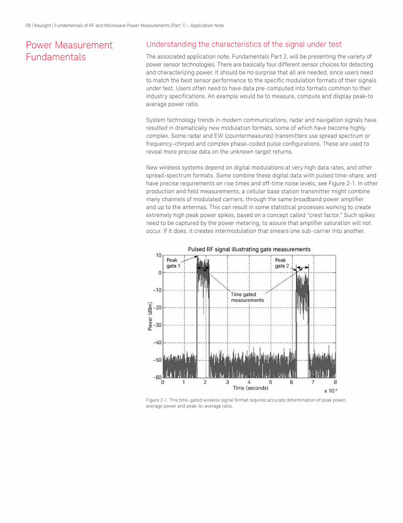
New wireless systems depend on digital modulations at very high data rates, and other

spread-spectrum formats. Some combine these digital data with pulsed time-share, and have precise requirements on rise times and off-time noise levels, see Figure 2-1. In other

production and ield measurements, a cellular base station transmitter might combine many channels of modulated carriers, through the same broadband power ampliier and up to the antennas. This can result in some statistical processes working to create

extremely high peak power spikes, based on a concept called “crest factor.” Such spikes need to be captured by the power metering, to assure that ampliier saturation will not occur. If it does, it creates intermodulation that smears one sub-carrier into another.

Power Measurement Fundamentals

Figure 2-1. This time-gated wireless signal format requires accurate determination of peak power,

average power and peak-to-average ratio.


Multiple signals, whether intentional or unintentional always stress a power sensor’s ability to integrate power, or to capture the modulation envelope. Average power sensors

such as thermistors and thermocouples inherently capture all power. No matter what

the format, they respond to the heat generated by the signal under test. Diode sensors,

feature much more sensitivity and dynamic range, but their conversion characteristic

ranges from square law detection (input power proportional to output voltage) through a

quasi-squarelaw region, to a linear region (input voltage proportional to output voltage).

Thus diode sensors can often be substituted for thermal sensors within their square-law

range, but if peak power or crest factors caused spikes of RF/microwave to exceed the square-law range, data errors will result. Diode sensors are the only choice for

characterizing pulsed waveform modulation envelopes or time-dependent formats

like spread-spectrum used in wireless systems.

Modern peak and average diode sensors are pre-calibrated for operation across a wide

dynamic range from square-law through the transition region to linear detection. They

do it by capturing calibration data and storing it internal to the sensor component in an

EEPROM. This correction data is then accessed for the inal digital readout of the asso-

ciated instrument. Diode calibration data also includes corrections for the all-important

sensitivity to temperature environments. Complete information on peak and average

diode sensors is given in Fundamentals Part 2.


Units and deinitions

WattThe International System of Units (SI) has established the watt (W) as the unit of power; one watt is one joule per second. Interestingly, electrical quantities do not even enter

into this deinition of power. In fact, other electrical units are derived from the watt. A volt is one watt per ampere. By the use of appropriate standard preixes the watt becomes the kilowatt (1 kW = 103 W), milliwatt (1 mW = 10-3 W), microwatt

(1 μW = 10-6 W), nanowatt (1 nW = 10-9 W), etc.

dBIn many cases, such as when measuring gain or attenuation, the ratio of two powers, or

relative power, is frequently the desired quantity rather than absolute power. Relative

power is the ratio of one power level, P, to some other level or reference level, Pref .

The ratio is dimensionless because the units of both the numerator and denominator

are watts. Relative power is usually expressed in decibels (dB).

The dB is deined by

dB = 10 log10 ( P ) (Equation 2-1) Pref

The use of dB has two advantages. First, the range of numbers commonly used is more

compact; for example +63 dB to –153 dB is more concise than 2 x 106 to 0.5 x 10-15. The

second advantage is apparent when it is necessary to ind the gain of several cascaded devices. Multiplication of numeric gain is then replaced by the addition of the power gain

in dB for each device.

dBmPopular usage has added another convenient unit, dBm. The formula for dBm is similar

to the dB formula except that the denominator, Pref, is always one milliwatt:

dB = 10 log10 ( P ) (Equation 2-2) 1 mW

In this expression, P is expressed in milliwatts and is the only variable, so dBm is used as a

measure of absolute power. An oscillator, for example, may be said to have a power output

of 13 dBm. By solving for P using the dBm equation, the power output can also be ex-

pressed as 20 mW. So dBm means “dB above one milliwatt” (no sign is assumed positive) but a negative dBm is to be interpreted as “dB below one milliwatt.” The advantages of the

term dBm parallel those for dB; it uses compact numbers and allows the use of addition

instead of multiplication when cascading gains or losses in a transmission system.

PowerThe term “average power” is very popular and is used in specifying almost all RF and

microwave systems. The terms “pulse power” and “peak envelope power” are more

pertinent to radar and navigation systems, and recently, TDMA signals in wireless

communication systems.

In elementary theory, power is said to be the product of voltage (V) and current (I). But

for an AC voltage cycle, this product V x I varies during the cycle as shown by curve P

in Figure 2-2, according to a 2f relationship. From that example, a sinusoidal generator

produces a sinusoidal current as expected, but the product of voltage and current has a

DC term as well as a component at twice the generator frequency. The word “power” as

most commonly used, refers to that DC component of the power product.

All the methods of measuring power to be discussed (except for one chapter on peak

power measurement) use power sensors which, by averaging, respond to the DC

component. Peak power instruments and sensors have time constants in the sub-

microsecond region, allowing measurement of pulsed power modulation envelopes.


The fundamental deinition of power is energy per unit time. This corresponds with the deinition of a watt as energy transfer at the rate of one joule per second. The important question to resolve is over what time is the energy transfer rate to be averaged when

measuring or computing power? From Figure 2-2 it is clear that if a narrow time interval

is shifted around within one cycle, varying answers for energy transfer rate are found.

But at radio and microwave frequencies, such microscopic views of the voltage-current

product are not common. For this application note, power is deined as the energy transfer per unit time averaged over many periods of the lowest frequency (RF or

microwave) involved.

A more mathematical approach to power for a continuous wave (CW) is to ind the average height under the curve of P in Figure 2-2. Averaging is done by inding the area under the curve, that is by integrating, and then dividing by the length of time over which

that area is taken. The length of time should be an exact number of AC periods. The

power of a CW signal at frequency (l/T0 ) is:

1

nT0 2π

2π

P = ——— ∫ ep sin (—— t)@ ip sin (—— + φ) (Equation 2-3) nT0

0

T0 T0

where T0 is the AC period, ep and ip represent peak values of e and i, φ is the phase angle

between e and i, and n is the number of AC periods. This yields (for n = 1, 2, 3 . . .):

P = epip

cos φ (Equation 2-4) 2

If the integration time is many AC periods long, then, whether or not n is a precise

integer makes a vanishingly small difference. This result for large n is the basis of power

measurement.

For sinusoidal signals, circuit theory shows the relationship between peak and rms values as:

__ __ ep = √2 Erms and ip = √2 Irms (Equation 2-5)

Using these in (2-4) yields the familiar expression for power:

P = Erms @ Irms cos φ (Equation 2-6)

Figure 2-2. The product of voltage and current, P, varies during the sinusoidal cycle.

DC component

e

P

Am

plitu

de

R

e

i

t

i


Average powerAverage power, like the other power terms to be deined, places further restrictions on the averaging time than just “many periods of the highest frequency.” Average power

means that the energy transfer rate is to be averaged over many periods of the lowest

frequency involved. For a CW signal, the lowest frequency and highest frequency are the

same, so average power and power are the same. For an amplitude modulated wave, the

power must be averaged over many periods of the modulation component of the signal

as well.

In a more mathematical sense, average power can be written as:

1

nTℓ

Pavg = —— — ∫ e(t) @ i(t)dt (Equation 2-7)

nT 0

where T is the period of the lowest frequency component of e(t) and i(t). The averaging

time for average power sensors and meters is typically from several hundredths of a

second to several seconds and therefore this process obtains the average of most

common forms of amplitude modulation.

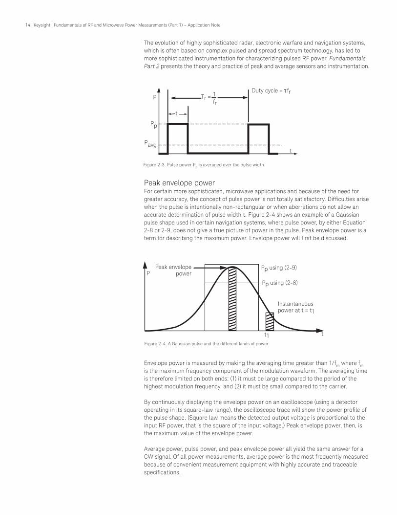
Pulse powerFor pulse power, the energy transfer rate is averaged over the pulse width, t. Pulse width

1 is considered to be the time between the 50% risetime/ fall-time amplitude points.

Mathematically, pulse power is given by:

1

t

Pp = —— ∫ e(t) @ i(t)dt (Equation 2-8)

t

0

By its very deinition, pulse power averages out any aberrations in the pulse envelope such as overshoot or ringing. For this reason it is called pulse power and not peak power

or peak pulse power as is done in many radar references. The terms peak power and

peak pulse power are not used here for that reason. Building on IEEE video pulse deini-tions, pulse-top amplitude also describes the pulse-top power averaged over its pulse

width. Peak power refers to the highest power point of the pulse top, usually the risetime

overshoot. See IEEE deinitions below.

The deinition of pulse power has been extended since the early days of microwave to be:

Pp = Pavg

(Equation 2-9)

Duty cycle

where duty cycle is the pulse width times the repetition frequency. See Figure 2-3. This extended deinition, which can be derived from Equations 2-7 and 2-8 for rectangular pulses, allows calculation of pulse power from an average power measurement and the

duty cycle.

For microwave systems which are designed for a ixed duty cycle, peak power is often calculated by use of the duty cycle calculation along with an average power sensor. See Figure 2-3. One reason is that the instrumentation is less expensive, and in a technical sense, the averaging technique integrates all the pulse imperfections into the average.


The evolution of highly sophisticated radar, electronic warfare and navigation systems,

which is often based on complex pulsed and spread spectrum technology, has led to

more sophisticated instrumentation for characterizing pulsed RF power. Fundamentals

Part 2 presents the theory and practice of peak and average sensors and instrumentation.

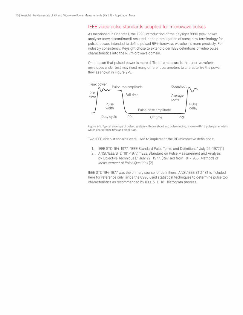
Figure 2-4. A Gaussian pulse and the different kinds of power.

Figure 2-3. Pulse power Pp is averaged over the pulse width.

Peak envelope powerFor certain more sophisticated, microwave applications and because of the need for

greater accuracy, the concept of pulse power is not totally satisfactory. Dificulties arise when the pulse is intentionally non-rectangular or when aberrations do not allow an

accurate determination of pulse width t. Figure 2-4 shows an example of a Gaussian

pulse shape used in certain navigation systems, where pulse power, by either Equation

2-8 or 2-9, does not give a true picture of power in the pulse. Peak envelope power is a

term for describing the maximum power. Envelope power will irst be discussed.

Envelope power is measured by making the averaging time greater than 1/fm where fm

is the maximum frequency component of the modulation waveform. The averaging time

is therefore limited on both ends: (1) it must be large compared to the period of the

highest modulation frequency, and (2) it must be small compared to the carrier.

By continuously displaying the envelope power on an oscilloscope (using a detector

operating in its square-law range), the oscilloscope trace will show the power proile of the pulse shape. (Square law means the detected output voltage is proportional to the input RF power, that is the square of the input voltage.) Peak envelope power, then, is

the maximum value of the envelope power.

Average power, pulse power, and peak envelope power all yield the same answer for a

CW signal. Of all power measurements, average power is the most frequently measured because of convenient measurement equipment with highly accurate and traceable

speciications.

t

P

Pp

Pavg

Tr = Duty cycle = t fr 1

fr

t

Peak envelopepowerP

Pp using (2-9)

Pp using (2-8)

Instantaneouspower at t = t1

t1 t


IEEE video pulse standards adapted for microwave pulses

As mentioned in Chapter I, the 1990 introduction of the Keysight 8990 peak power

analyzer (now discontinued) resulted in the promulgation of some new terminology for

pulsed power, intended to deine pulsed RF/microwave waveforms more precisely. For industry consistency, Keysight chose to extend older IEEE deinitions of video pulse characteristics into the RF/microwave domain.

One reason that pulsed power is more dificult to measure is that user-waveform envelopes under test may need many different parameters to characterize the power

low as shown in Figure 2-5.

Two IEEE video standards were used to implement the RF/microwave deinitions:

1. IEEE STD 194-1977, “IEEE Standard Pulse Terms and Deinitions,” July 26, 1977.[1]2. ANSI/IEEE STD 181-1977, “IEEE Standard on Pulse Measurement and Analysis

by Objective Techniques,” July 22, 1977. (Revised from 181-1955, Methods of

Measurement of Pulse Qualities.[2]

IEEE STD 194-1977 was the primary source for deinitions. ANSI/IEEE STD 181 is included here for reference only, since the 8990 used statistical techniques to determine pulse top

characteristics as recommended by IEEE STD 181 histogram process.

Figure 2-5. Typical envelope of pulsed system with overshoot and pulse ringing, shown with 13 pulse parameters

which characterize time and amplitude.

Peak powerPulse-top amplitude Overshoot

PRF

Fall timeRise time

Pulse width

Duty cycle PRI

Pulse-base amplitude

Off time

Pulsedelay

Averagepower


It was recognized that while terms and graphics from both those standards were written

for video pulse characteristics, most of the measurement theory and intent of the deini-tions can be applied to the waveform envelopes of pulse-modulated RF and microwave

carriers. Several obvious exceptions would be parameters such as pre-shoot, which is the negative-going undershoot that precedes a pulse risetime. Negative power would be

meaningless. The same reasoning would apply to the undershoot following the fall time

of a pulse.

For measurements of pulse parameters such as risetime or overshoot to be meaningful,

the points on the waveform that are used in the measurement must be deined unambig-

uously. Since all the time parameters are measured between speciic amplitude points on the pulse, and since all the amplitude points are referenced to the two levels named

“top” and “base,” Figure 2-6 shows how they are deined.

Figure 2-6. IEEE pulse deinitions and standards for video parameters applied to microwave pulse envelopes. ANSI/IEEE Std 194-1977, Copyright © 1977, IEEE all rights reserved.


Peak power waveform deinitionsThe following are deinitions for 13 RF pulse parameters as adapted from IEEE video deinitions:

Rise time The time difference between the proximal and distal irst transition points, usually 10 and 90% of pulse-top amplitude (vertical display is

linear power).

Fall time Same as risetime measured on the last transition.

Pulse width The pulse duration measured at the mesial level; normally taken as the

50% power level.

Off time Measured on the mesial (50%) power line; pulse separation, the interval between the pulse stop time of a irst pulse waveform and the pulse start time of the immediately following pulse waveform in a pulse train.

Duty cycle The previously measured pulse duration divided by the pulse repetition

interval.

PRI (Pulse repetition interval) The interval between the pulse start time

of a irst pulse waveform and the pulse start time of the immediately following pulse waveform in a periodic pulse train.

PRF (pulse repetition frequency) The reciprocal of PRI.

Pulse delay The occurrence in time of one pulse waveform before (after) another

pulse waveform; usually the reference time would be a video system

timing or clock pulse.

Pulse-top Pulse amplitude, deined as the algebraic amplitude difference between the top magnitude and the base magnitude; calls for a speciic procedure or algorithm, such as the histogram method.1

Pulse-base The pulse waveform baseline speciied to be obtained by the histogram algorithm.

Peak power The highest point of power in the waveform, usually at the irst over-shoot; it might also occur elsewhere across the pulse top if parasitic

oscillations or large amplitude ringing occurs; peak power is not the

pulse-top amplitude which is the primary measurement of pulse

amplitude.

Overshoot A distortion that follows a major transition; the difference between the peak power point and the pulse-top amplitude computed as a

percentage of the pulse-top amplitude.

Average power Computed by using the statistical data from pulse-top amplitude power

and time measurements.

1. In such a method, the probability histogram of power samples is computed. This is split in two around the mesial line and yields a peak in each segment. Either the mode or the mean of these histograms gives the pulse top and pulse bottom power.


A typical wireless modulation format

Modern wireless system designs use TDMA (time division multiple access) and CDMA

(code division multiple access) for combining many channels into broadband complex

signal formats. For the typical signal of Figure 2-1, the EDGE system (enhanced data rate

for GSM evolution) requires a characterization of peak, average and peak-to-average ratios during the pulse-burst interval.

The power sensor used must faithfully capture the fast rise/fall times of the system pulse, plus respond to the digital phase modulation in the time gate, without being

inluenced by the statistical crest factor spikes of the modulation. To render the power metering instrumentation insensitive to off-time noise, the instrument requires a

time-gating function which can capture data during speciied time intervals.

Modern digital computation routines provide for peak-to-average determinations.

Design engineers can obtain more complicated statistical data such as the CCDF, a

distribution function which states the percentage of the time a wireless signal is larger

than a speciied value. This is of great value in testing and troubleshooting non-linearity of power ampliiers.[3]

Three technologies for sensing power

There are three popular devices for sensing and measuring average power at RF and

microwave frequencies. Each of the methods uses a different kind of device to convert

the RF power to a measurable DC or low frequency signal. The devices are the thermistor,

the thermocouple, and the diode detector. Each of the next three chapters discusses

in detail one of those devices and its associated instrumentation. Fundamentals Part 2

discusses diode detectors used to measure pulsed and complex modulation envelopes.

Each method has some advantages and disadvantages over the others. After the individual

measurement sensors are studied, the overall measurement errors are discussed in

Fundamentals Part 2.

The general measurement technique for average power is to attach a properly calibrated

sensor to the transmission line port at which the unknown power is to be measured. The

output from the sensor is connected to an appropriate power meter. The RF power to

the sensor is turned off and the power meter zeroed. This operation is often referred to

as “zero setting” or “zeroing.” Power is then turned on. The sensor, reacting to the new

input level, sends a signal to the power meter and the new meter reading is observed.


An overview of power sensors and meters for pulsed and complex modulations

As the new wireless communications revolution of the 1990s took over, the need for

instruments to characterize the power envelope of complex digital modulation formats

led to the introduction of the Keysight E4416/17A peak and average power meters, and to the retirement of the 8990 meter. Complete descriptions of the new peak and

average sensors and meters along with envelope characterization processes known as

“time-gated” measurements are given in Fundamentals Part 2. “Time-gated” is a term

that emerged from spectrum analyzer applications. It means adding a time selective

control to the power measurement.

The E4416/17A peak and average meters also led to some new deinitions of pulsed parameters, suitable for the communications industry. For example, burst average

power is that pulsed power averaged across a TDMA pulse width. Burst average power

is functionally equivalent to the earlier pulse-top amplitude of Figure 2-5. One term serves the radar applications arena and the other, the wireless arena.

Key power sensor parameters

In the ideal measurement case above, the power sensor absorbs all the power incident

upon the sensor. There are two categories of non-ideal behavior that are discussed in

detail in Fundamentals Part 3, but will be introduced here.

First, there is likely an impedance mismatch between the characteristic impedance of

the RF source or transmission line and the RF input impedance of the sensor. Thus, some

of the power that is incident on the sensor is relected back toward the generator rather than dissipated in the sensor. The relationship between incident power Pi , relected power Pr , and dissipated power Pd , is:

Pi = Pr + Pd (Equation 2-10)

The relationship between Pi and Pr for a particular sensor is given by the sensor relection coeficient magnitude P

ℓ.

Pr = rℓ2 + Pi (Equation 2-11)

Relection coeficient magnitude is a very important speciication for a power sensor because it contributes to the most prevalent source of error, mismatch uncertainty,

which is discussed in Fundamentals Part 3. An ideal power sensor has a relection coeficient of zero, no mismatch. While a r

ℓ of 0.05 or 5% (equivalent to an SWR of

approximately 1.11) is preferred for most situations, a 50% relection coeficient would not be suitable for most situations due to the large measurement uncertainty it causes.

Some early waveguide sensors were speciied at a relection coeficient of 0.35.


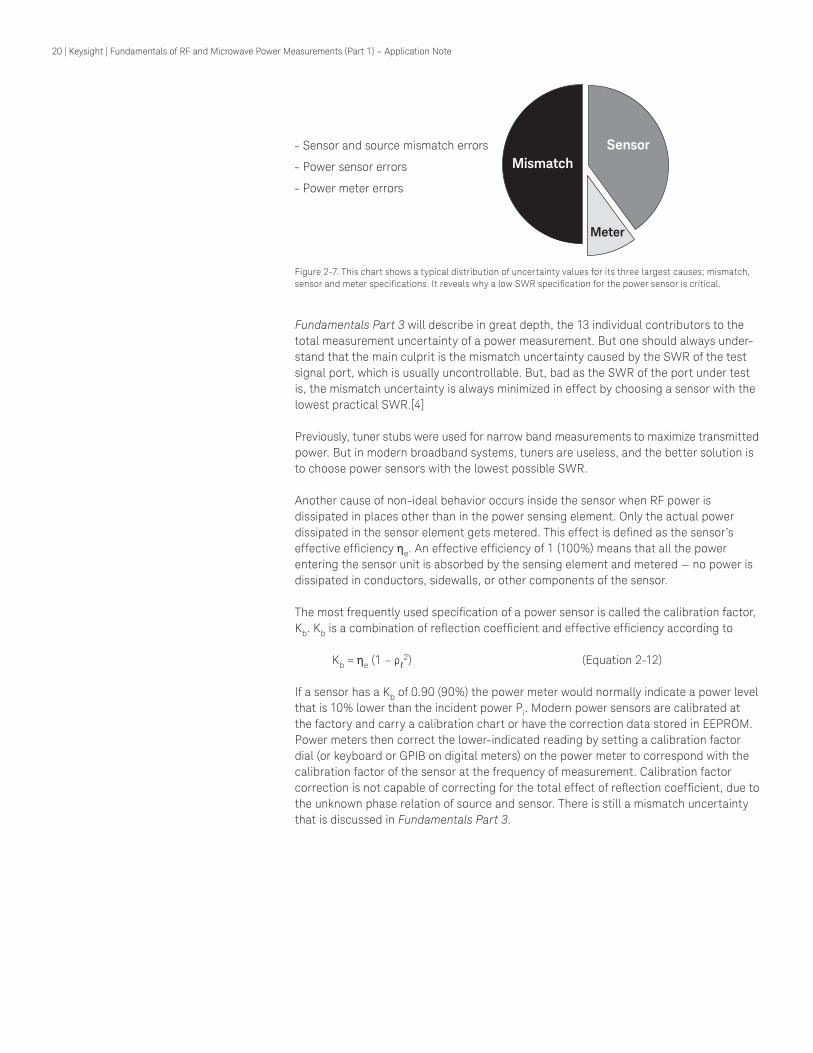
Fundamentals Part 3 will describe in great depth, the 13 individual contributors to the

total measurement uncertainty of a power measurement. But one should always under-

stand that the main culprit is the mismatch uncertainty caused by the SWR of the test signal port, which is usually uncontrollable. But, bad as the SWR of the port under test is, the mismatch uncertainty is always minimized in effect by choosing a sensor with the

lowest practical SWR.[4]

Previously, tuner stubs were used for narrow band measurements to maximize transmitted

power. But in modern broadband systems, tuners are useless, and the better solution is

to choose power sensors with the lowest possible SWR.

Another cause of non-ideal behavior occurs inside the sensor when RF power is

dissipated in places other than in the power sensing element. Only the actual power dissipated in the sensor element gets metered. This effect is deined as the sensor’s effective eficiency he. An effective eficiency of 1 (100%) means that all the power entering the sensor unit is absorbed by the sensing element and metered — no power is

dissipated in conductors, sidewalls, or other components of the sensor.

The most frequently used speciication of a power sensor is called the calibration factor, Kb. Kb is a combination of relection coeficient and effective eficiency according to

Kb = he (1 – ρℓ2) (Equation 2-12)

If a sensor has a Kb of 0.90 (90%) the power meter would normally indicate a power level

that is 10% lower than the incident power Pi. Modern power sensors are calibrated at

the factory and carry a calibration chart or have the correction data stored in EEPROM. Power meters then correct the lower-indicated reading by setting a calibration factor

dial (or keyboard or GPIB on digital meters) on the power meter to correspond with the

calibration factor of the sensor at the frequency of measurement. Calibration factor

correction is not capable of correcting for the total effect of relection coeficient, due to the unknown phase relation of source and sensor. There is still a mismatch uncertainty

that is discussed in Fundamentals Part 3.

Figure 2-7. This chart shows a typical distribution of uncertainty values for its three largest causes; mismatch, sensor and meter speciications. It reveals why a low SWR speciication for the power sensor is critical.

– Sensor and source mismatch errors

– Power sensor errors

– Power meter errors

Mismatch

Sensor

Meter


Data computation for statistical parameters of power analysis

With the advent of Keysight digital sampling power meters such as the E4416A/17A models, massive amounts of digital data can be harnessed to deliver power parameters

far more complex than average or peak power. Since many system modulations are characterized by noisy or digitally complex envelopes, digital data points are ideal for

providing computed results in formats useful to the customer.

A typical noisy waveform might be the combined channel output from a wireless base

station power ampliier. For operating eficiency, many wireless channels are multi-plexed onto a single output power stage. This technique works very well as long as the

power ampliier is not overdriven with crest factor signal spikes that move up out of the linear ampliier portion of the transmitter. This then presents the station installation and maintenance personnel with the responsibility of assuring the power data indicates the

ampliier linearity has not been exceeded.

Modern power meters like the E4417A with appropriate computational software can process the digital data to display such power parameters as the CCDF (complementary

cumulative distribution function). This parameter is critically important to design

engineers who need to know what percentage of the time their peak-to-average ratio

is above a speciied signal level.[5]

[1] IEEE STD 194-1977, “IEEE Standard Pulse Terms and Deinitions,” (July 26, 1977), IEEE, New York, NY.

[2] ANSI/IEEE STD181-1977, “IEEE Standard on Pulse Measurement and Analysis by Objective Techniques,” July 22, 1977. Revised from 181-1955, Methods of

Measurement of Pulse Qualities, IEEE, New York, NY.

[3] Anderson, Alan, “Measuring Power Levels in Modern Communications Systems,” Microwaves/RF, October 2000.

[4] Lymer, Anthony, “Improving Measurement Accuracy by Controlling Mismatch Uncertainty” TechOnLine, September 2002. Website: www.techonline.com

[5] Breakenridge, Eric, “Use a Sampling Power Meter to Determine the Characteristics of RF and Microwave Devices,” Microwaves/RF, September 2001


The hierarchy of power measurements, national standards and traceability

Since power measurement has important commercial ramiications, it is important that power measurements can be duplicated at different times and at different places. This

requires well-behaved equipment, good measurement technique, and common agreement

as to what is the standard watt. The agreement in the United States is established by the National Institute of Standards and Technology (NIST) at Boulder, Colorado, which main-

tains a National Reference Standard in the form of various microwave microcalorimeters for different frequency bands.[1, 2] When a power sensor can be referenced back to that

National Reference Standard, the measurement is said to be traceable to NIST.

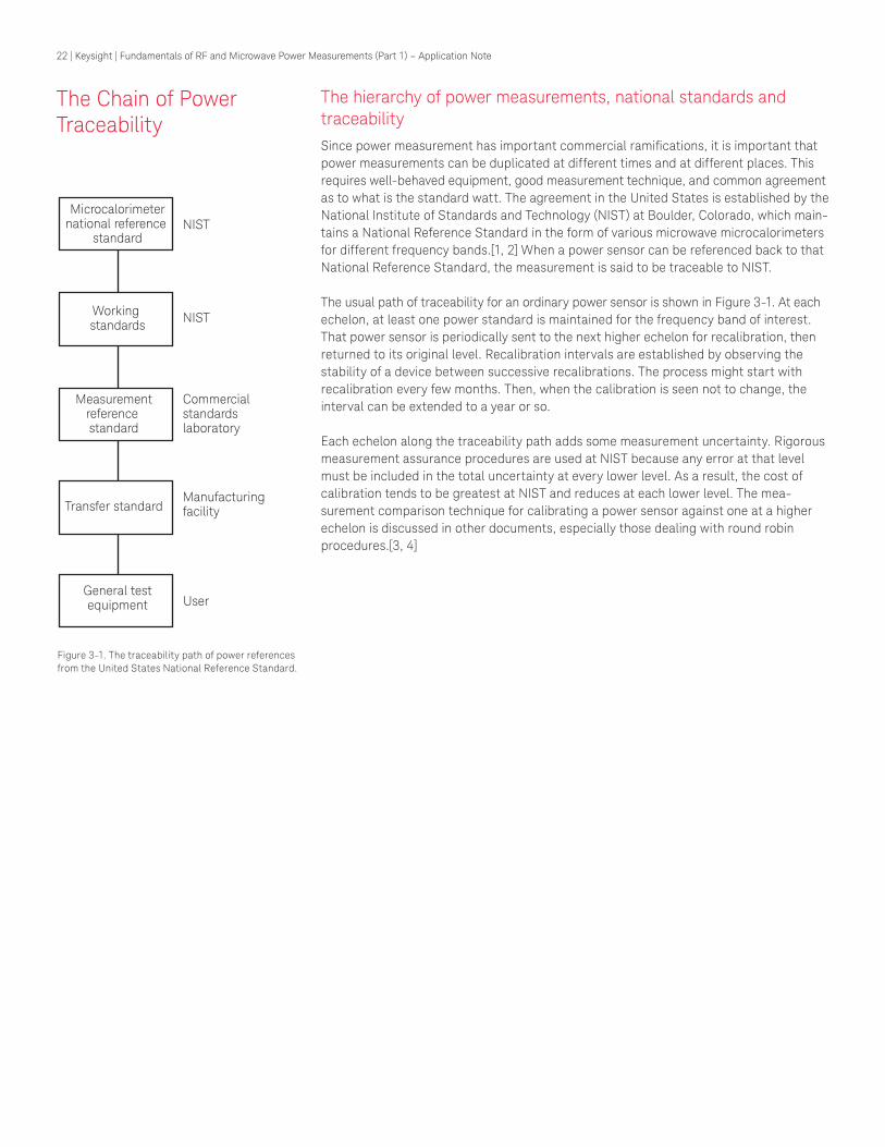
The usual path of traceability for an ordinary power sensor is shown in Figure 3-1. At each

echelon, at least one power standard is maintained for the frequency band of interest.

That power sensor is periodically sent to the next higher echelon for recalibration, then

returned to its original level. Recalibration intervals are established by observing the

stability of a device between successive recalibrations. The process might start with

recalibration every few months. Then, when the calibration is seen not to change, the

interval can be extended to a year or so.

Each echelon along the traceability path adds some measurement uncertainty. Rigorous

measurement assurance procedures are used at NIST because any error at that level must be included in the total uncertainty at every lower level. As a result, the cost of

calibration tends to be greatest at NIST and reduces at each lower level. The mea-

surement comparison technique for calibrating a power sensor against one at a higher

echelon is discussed in other documents, especially those dealing with round robin

procedures.[3, 4]

The Chain of Power Traceability

Figure 3-1. The traceability path of power references

from the United States National Reference Standard.

NIST

NIST

Commercial standards laboratory

Manufacturingfacility

User

Working standards

Measurementreference standard

Transfer standard

Microcalorimeternational reference

standard

General testequipment


The National Power Reference Standard for the U.S. is a microcalorimeter maintained at the NIST in Boulder, CO, for the various coaxial and waveguide frequency bands offered in their measurement services program. These measurement services are described in

NIST SP-250, available from NIST on request.[5] They cover coaxial mounts from 10 MHz to 50 GHz and waveguide from 18 GHz to the high millimeter ranges of 96 GHz.

A microcalorimeter measures the effective eficiency of a DC substitution sensor which is then used as the transfer standard. Microcalorimeters operate on the principle that after

applying an equivalence correction, both DC and absorbed microwave power generate

the same heat. Comprehensive and exhaustive analysis is required to determine the

equivalence correction and account for all possible thermal and RF errors, such as losses

in the transmission lines and the effect of different thermal paths within the microcalori-

meter and the transfer standard. The DC-substitution technique is used because the

fundamental power measurement can then be based on DC voltage (or current) and

resistance standards. The traceability path leads through the microcalorimeter (for

effective eficiency, a unit-less correction factor) and inally back to the national DC standards.

In addition to national measurement services, other industrial organizations often

participate in comparison processes known as round robins (RR). A RR provides mea-

surement reference data to a participating lab at very low cost compared to primary

calibration processes. For example, the National Conference of Standards Laboratories International (NCSLI), a non-proit association of over 1400 world-wide organizations, maintains RR projects for many measurement parameters, from dimensional to optical.

The NCSLI Measurement Comparison Committee oversees those programs.[3]

For RF power, a calibrated thermistor mount starts out at a “pivot lab,” usually one with

overall RR responsibility, then travels to many other reference labs to be measured,

returning to the pivot lab for closure of measured data. Such mobile comparisons are also carried out between National Laboratories of various countries as a routine procedure to assure international measurements at the highest level.

Microwave power measurement calibration services are available from many National

Laboratories around the world, such as the NPL in the United Kingdom and PTB in Germany. Calibration service organizations are numerous too, with names like NAMAS in the United Kingdom.

Figure 3-2. Schematic cross-section of the NIST coaxial microcalorimeter at Boulder, CO. The entire sensor coniguration is maintained under a water bath with a highly-stable temperature so that RF

to DC substitutions may be made precisely.


The theory and practice of sensor calibration

Every power sensor, even the DC-substitution types such as thermistor types, require

data correction for frequency response, temperature effects, substitution errors from

RF to DC, or conversion and heating effects. The ultimate power standard is usually a

microcalorimeter at a NMI, for example, in the United States, the NIST, as described previously. By carefully transferring the microcalorimeter power measurement data to

secondary standard sensors, the NMIs can supply comparison services to customer

sensors. These are transportable between the NMI and their organization’s primary standards labs, and in turn, down to the production line or ield measurement.

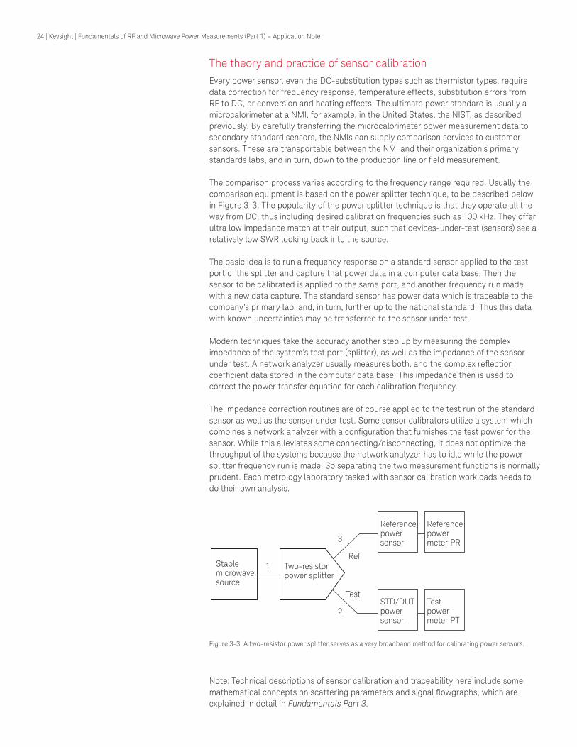
The comparison process varies according to the frequency range required. Usually the

comparison equipment is based on the power splitter technique, to be described below

in Figure 3-3. The popularity of the power splitter technique is that they operate all the

way from DC, thus including desired calibration frequencies such as 100 kHz. They offer

ultra low impedance match at their output, such that devices-under-test (sensors) see a

relatively low SWR looking back into the source.

The basic idea is to run a frequency response on a standard sensor applied to the test

port of the splitter and capture that power data in a computer data base. Then the

sensor to be calibrated is applied to the same port, and another frequency run made

with a new data capture. The standard sensor has power data which is traceable to the

company’s primary lab, and, in turn, further up to the national standard. Thus this data with known uncertainties may be transferred to the sensor under test.

Modern techniques take the accuracy another step up by measuring the complex

impedance of the system’s test port (splitter), as well as the impedance of the sensor under test. A network analyzer usually measures both, and the complex relection coeficient data stored in the computer data base. This impedance then is used to correct the power transfer equation for each calibration frequency.

The impedance correction routines are of course applied to the test run of the standard

sensor as well as the sensor under test. Some sensor calibrators utilize a system which combines a network analyzer with a coniguration that furnishes the test power for the sensor. While this alleviates some connecting/disconnecting, it does not optimize the throughput of the systems because the network analyzer has to idle while the power

splitter frequency run is made. So separating the two measurement functions is normally prudent. Each metrology laboratory tasked with sensor calibration workloads needs to

do their own analysis.

Figure 3-3. A two-resistor power splitter serves as a very broadband method for calibrating power sensors.

Stablemicrowavesource

1

2

3

Two-resistorpower splitter

Ref

Test

Referencepower sensor

Referencepower meter PR

STD/DUTpower sensor

Testpower meter PT

Note: Technical descriptions of sensor calibration and traceability here include some

mathematical concepts on scattering parameters and signal lowgraphs, which are explained in detail in Fundamentals Part 3.


Some measurement considerations for power sensor comparisonsFor metrology users involved in the acquisition, routine calibration, or roundrobin

comparison processes for power sensors, an overview might be useful. Since thermistor sensors are most often used as the transfer reference, the processes will be discussed

in this section.

Typical sensor comparison system

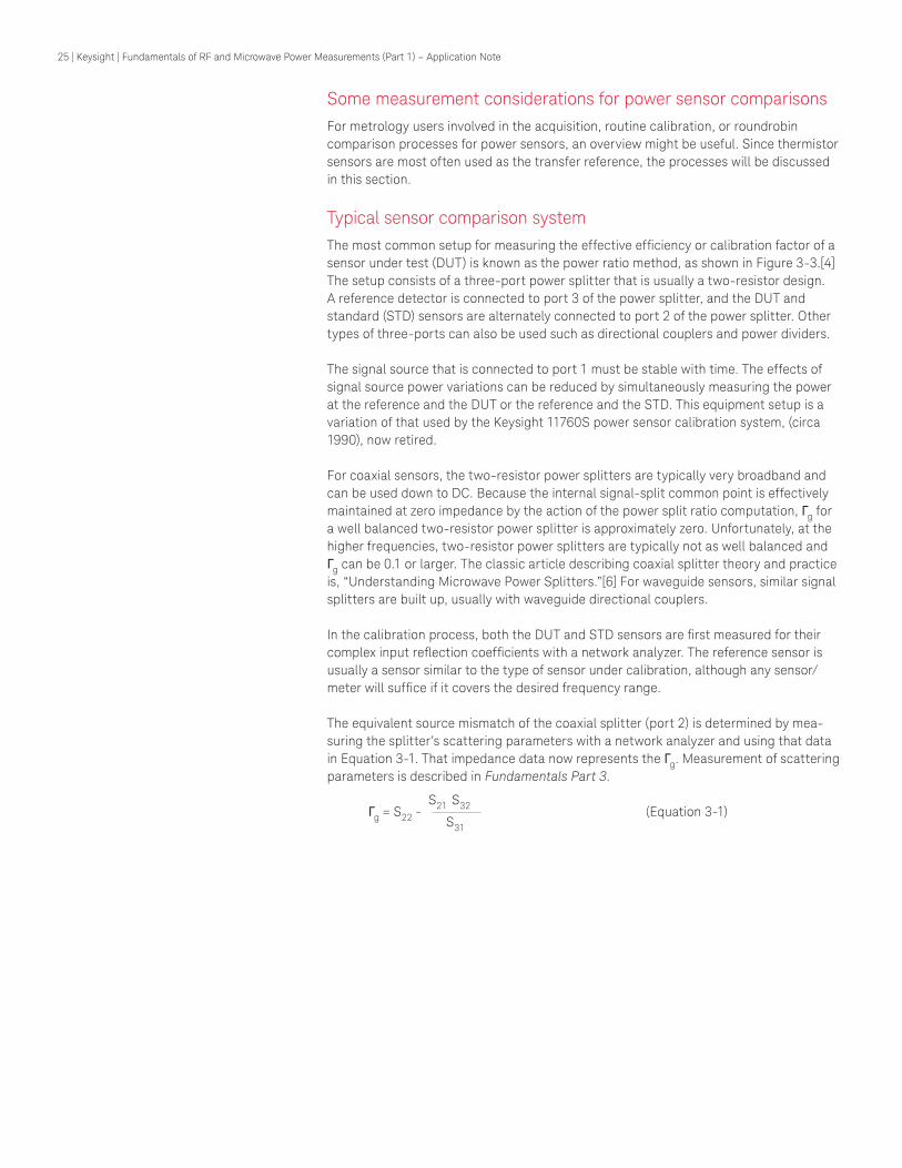
The most common setup for measuring the effective eficiency or calibration factor of a sensor under test (DUT) is known as the power ratio method, as shown in Figure 3-3.[4]

The setup consists of a three-port power splitter that is usually a two-resistor design.

A reference detector is connected to port 3 of the power splitter, and the DUT and

standard (STD) sensors are alternately connected to port 2 of the power splitter. Other types of three-ports can also be used such as directional couplers and power dividers.

The signal source that is connected to port 1 must be stable with time. The effects of

signal source power variations can be reduced by simultaneously measuring the power

at the reference and the DUT or the reference and the STD. This equipment setup is a variation of that used by the Keysight 11760S power sensor calibration system, (circa 1990), now retired.

For coaxial sensors, the two-resistor power splitters are typically very broadband and

can be used down to DC. Because the internal signal-split common point is effectively

maintained at zero impedance by the action of the power split ratio computation, Gg for

a well balanced two-resistor power splitter is approximately zero. Unfortunately, at the

higher frequencies, two-resistor power splitters are typically not as well balanced and

Gg can be 0.1 or larger. The classic article describing coaxial splitter theory and practice

is, “Understanding Microwave Power Splitters.”[6] For waveguide sensors, similar signal splitters are built up, usually with waveguide directional couplers.

In the calibration process, both the DUT and STD sensors are irst measured for their complex input relection coeficients with a network analyzer. The reference sensor is usually a sensor similar to the type of sensor under calibration, although any sensor/

meter will sufice if it covers the desired frequency range.

The equivalent source mismatch of the coaxial splitter (port 2) is determined by mea-

suring the splitter’s scattering parameters with a network analyzer and using that data in Equation 3-1. That impedance data now represents the Gg. Measurement of scattering

parameters is described in Fundamentals Part 3.

Gg = S22 - S21 S32

(Equation 3-1)

S31


There is also a direct-calibration method for determining Gg, that is used at NIST.[7] Although this method requires some external software to set it up, it is easy to use once

it is up and running.

Next, the power meter data for the standard sensor and reference sensor are measured

across the frequency range, followed by the DUT and reference sensor. It should be

noted that there might be two different power meters used for the “test” meter, since a

Keysight 432 meter would be used if the STD sensor was a thermistor, while a Keysight EPM meter would be used to read the power data for a thermocouple DUT sensor. Then

these test power meter data are combined with the appropriate relection coeficients according to the equation:

PTdut PRstd |1 - Gg Gd|2

Kb = Ks ———————————————————— (Equation 3-2)

PTstd PRdut |1 - Gg Gs|2

Where:

Kb = cal factor of DUT sensor

Ks = cal factor of STD sensorPTdut = reading of test power meter with DUT sensor

PTstd = reading of test power meter with STD sensorPRstd = reading of reference power meter when STD measuredPRdut = reading of reference power meter when DUT measured

Gg = equivalent generator relection coeficient ρg= |Gg|

Gd = relection coeficient of DUT sensor ρd = |Gd|

Gs = relection coeficient of STD sensor ρs= |Gs|

A 75 Ω splitter might be substituted for the more common 50 Ω splitter if the DUT sensor is a 75 Ω unit.

Finally, it should also be remembered that the effective eficiency and calibration factor of thermocouple and diode sensors do not have any absolute power reference,

compared to a thermistor sensor. Instead, they depend on their 50 MHz reference source

to set the calibration level. This is relected by the Equation 3-2, which is simply a ratio.


Thermistors as power transfer standards

For special use as transfer standards, the U.S. NIST, accepts thermistor mounts, both coaxial and waveguide, to transfer power parameters such as calibration factor, effective

eficiency and relection coeficient in their measurement services program. To provide those services below 100 MHz, NIST instructions require sensors specially designed for that performance.

One example of a special power calibration transfer is the one required to precisely calibrate the internal 50 MHz, 1 mW power standard in the Keysight power meters,

which use a family of thermocouples or diode sensors. That internal power reference is

needed since those sensors do not use the power substitution technique. For standard-

izing the 50 MHz power reference, a specially-modiied Keysight 478A thermistor sensor with a larger RF coupling capacitor is available for operation from 1 MHz to 1 GHz. It is

designated the 478A Special Option H55 and features an SWR of 1.35 over its range. For an even lower transfer uncertainty at 50 MHz, the 478A Special Option H55 can be selected for 1.05 SWR at 50 MHz. This selected model is designated the 478A Special Option H75.

478A Special Option H76 thermistor sensor is the H75 sensor that has been specially calibrated in the Keysight Microwave Standards Lab with a 50 MHz power reference traceable to NIST. Other coaxial and waveguide thermistor sensors are available for metrology use.

NIST sensor calibration services while mainly focused on DC-substitution technology using thermistor sensors ran out of frequency range at the upper limit of coaxial

thermistors. NIST now offers calibration service for thermocouple sensors that reach 50 GHz.[5]

Other DC-substitution metersOther self-balancing power meters can also be used to drive thermistor sensors for measurement of power. In particular, the NIST Type 4 power meter, designed by the NIST for high-accuracy measurement of microwave power is well suited for the purpose. The

Type 4 meter uses automatic balancing, along with a four-terminal connection to the

thermistor sensor and external high precision DC voltage instrumentation. This permits

lower uncertainty than commercial power meters are designed to accomplish


Peak power sensor calibration traceability

For years, ultimate power sensor traceability to national standards was limited to average

power parameters. One can understand this because the microcalorimeter-based standard inherently depends on a long-term power absorption at very stable signal

conditions. With the very long time-constants of microcalorimeters, the process calls

for characterizing the power transfer for a long averaging period.

The average power of real-world signal formats is seldom the only parameter of interest.

New wireless communications signals combine multiplexed channels that look like noise

power with pulsed formats for time-share. The EDGE signal of Figure 2-1 is a good

example. Naturally, manufacturers and users of peak power sensors would be requesting

traceability for such special formats.

As of this writing, the National Physical Laboratory (NPL) in the UK has sponsored a research program into the complexities of characterizing peak power sensors. These

are not trivial considerations because bandwidth of the instrumentation and the linearity

of the sensor both contribute to computed errors. In particular, the linearity of peak-

detecting sensors at low power levels was generally poorer than CW sensors. Peak

sensors also reveal more nonlinearities in the higher power areas where corrections are

applied to the detection characteristic. Range-switching transitions can lead to minor

data discontinuities. These all can lead to uncertainties in computed data such as

peak-to-average power and power statistics which are required for CDMA systems like

cdmaOne and W-CDMA.

The NPL calibration system work was validated against the sampling oscilloscope measurements that validated the waveform characteristics of the pulsed RF signal.

This is important because of the generally limited bandwidth of the peak power instru-

mentation associated with pulsed or complex-modulation power signals. Of course, the ultimate power standard was still a CW sensor, which served as the traceable link to the

NPL power standard.

NPL’s peak power project has involved various popular frequency bands and power levels. It is suggested that potential users of peak power sensor calibration services

make direct contact with the NPL website.[10]

In a summary presentation for peak power uncertainty budget for a DECT signal

(1900 MHz region), the total was computed at a 3.2% uncertainty for 95% conidence. The overall expanded uncertainty included sensor eficiency, power ratio, standard sensor mismatch, DUT sensor mismatch and repeatability, plus the CW—pulse transfer.


Network analyzer source method

For production situations, it is possible to modify an automatic RF/microwave network analyzer to serve as the test signal source, in addition to its primary duty measuring

impedance. The modiication is not a trivial process, however, due to the fact that the signal paths inside the analyzer test set sometimes do not provide adequate power

output to the test sensor because of directional coupler roll off.

NIST six-port calibration systemFor its calibration services of coaxial, waveguide, and power detectors, the NIST uses a number of different methods to calibrate power detectors. The primary standards

are calibrated in either coaxial or waveguide calorimeters.[9, 11] However, these mea-

surements are slow and require specially built detectors that have the proper thermal

characteristics for calorimetric measurements. For that reason the NIST calorimeters have historically been used to calibrate standards only for internal NIST use.

The calibration of detectors for NIST’s customers is usually done on either the dual six-port network analyzer or with a two-resistor power splitter setup such as the one

described above.[11] While different in appearance, both of these methods basically use

the same principles and therefore provide similar results and similar uncertainties.

The advantage of the dual six-ports is that they can measure Gg, Gs, and Gd, and the power

ratios in Equation 3-2 at the same time. The two-resistor power splitter setup requires

two independent measurement steps since Gg, Gs, and Gd are measured on a vector

network analyzer prior to the measurement of the power ratios. The disadvantage of the

dual six-ports is that the NIST systems typically use four different systems to cover the 10 MHz to 50 GHz frequency band. The advantage of the two-resistor power splitter is

its wide bandwidth and DC-50 GHz power splitters are currently commercially available.


1] J. Wade Allen, Fred R. Clague, Neil T. Larsen, and M. P. Weidman, “NIST Microwave Power Standards in Waveguide,” NIST Technical Note 1511, February 1999.

[2] F.R. Clague, “A Calibration Service for Coaxial Reference Standards for Microwave Power,” NIST Technical Note 1374, May, 1995.

[3] National Conference of Standards Laboratories, Measurement Comparison Committee, Suite 305B, 1800 30th St. Boulder, CO 80301.

[4] M.P. Weidman, “Direct Comparison Transfer of Microwave Power Sensor Calibration,” NIST Technical Note 1379, January, 1996.

[5] NIST Special Publication 250; NIST Calibration Services. The latest up-to-date information on NIST calibration services is also maintained on the following website: www.ts.nist.gov/ts/htdocs/230/233/calibrations/index.htm

[6] Russell A. Johnson, “Understanding Microwave Power Splitters,” Microwave Journal, Dec 1975.

[7] R.F. Juroshek, John R., “A direct calibration method for measuring equivalent source mismatch,” Microwave Journal, October 1997, pp 106-118.

[8] Clague, F. R. , and P. G. Voris, “Coaxial reference standard for microwave power,”

NIST Technical Note 1357, U. S. Department of Commerce, April 1993.[9] Allen, J.W., F.R. Clague, N.T. Larsen, and W. P Weidman, “NIST microwave power

standards in waveguide,” NIST Technical Note 1511, U. S. Department of Commerce, February 1999.

[10] Website for National Physics Laboratory, UK, pulsed power information (note caps): www.npl.co.uk/measurement_services/ms_EG.html#EG04

[11] Engen, G.F., “Application of an arbitrary 6-port junction to power-measurement

problems,” IEEE Transactions on Instrumentation and Measurement, Vol IM-21,

November 1972, pp 470-474.

General references

R.W. Beatty, “Intrinsic Attenuation,” IEEE Trans. on Microwave Theory and Techniques,

Vol. I I, No. 3 (May, 1963) 179-182.R.W. Beatty, “Insertion Loss Concepts,” Proc. of the IEEE. Vol. 52, No. 6 (June, 1966)

663-671.S.F. Adam, “Microwave Theory & Applications,” Prentice-Hall, 1969.C.G. Montgomery, “Technique of Microwave Measurements,” Massachusetts Institute of

Technology, Radiation Laboratory Series, Vol. 11. McGraw-Hill, Inc., 1948.Mason and Zimmerman. “Electronic Circuits, Signals and Systems,” John Wiley and

Sons, Inc., 1960.Fantom, A, “Radio Frequency & Microwave Power Measurements,” Peter Peregrinus Ltd,

1990

“IEEE Standard Application Guide for Bolometric Power Meters,” IEEE Std. 470-1972.“IEEE Standard for Electrothermic Power Meters,” IEEE Std. 544-1976.20

http://www.ts.nist.gov/ts/htdocs/230/233/calibrations/index.htm

http://www.npl.co.uk/measurement_services/ms_EG.html%23EG04


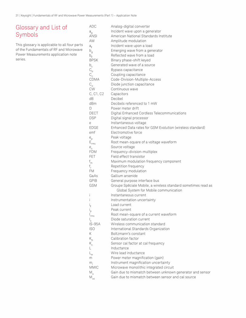
Glossary and List of Symbols

This glossary is applicable to all four parts

of the Fundamentals of RF and Microwave

Power Measurements application note

series.

ADC Analog-digital converter

ag Incident wave upon a generator

ANSI American National Standards InstituteAM Amplitude modulation

aℓ Incident wave upon a load

bg Emerging wave from a generator

bℓ Relected wave from a load

BPSK Binary phase-shift keyedbs Generated wave of a source

Cb Bypass capacitance

Cc Coupling capacitance

CDMA Code-Division-Multiple-Access

Co Diode junction capacitance

CW Continuous wave

C, C1, C2 Capacitors

dB Decibel

dBm Decibels referenced to 1 mW

D Power meter drift

DECT Digital Enhanced Cordless Telecommunications

DSP Digital signal processore Instantaneous voltage

EDGE Enhanced Data rates for GSM Evolution (wireless standard)emf Electromotive force

ep Peak voltage

Erms Root mean-square of a voltage waveform

es Source voltageFDM Frequency-division-multiplex

FET Field effect transistor

fm Maximum modulation frequency component

fr Repetition frequency

FM Frequency modulation

GaAs Gallium arsenide

GPIB General purpose interface bus

GSM Groupe Spêciale Mobile, a wireless standard sometimes read as Global System for Mobile communication

i Instantaneous current

i Instrumentation uncertainty

iℓ Load current

ip Peak current

Irms Root mean-square of a current waveform

Is Diode saturation current

IS-95A Wireless communication standardISO International Standards OrganizationK Boltzmann’s constantKb Calibration factor

Kc Sensor cal factor at cal frequencyL InductanceLw Wire lead inductance

m Power meter magniication (gain)mi Instrument magniication uncertaintyMMIC Microwave monolithic integrated circuit

Mu Gain due to mismatch between unknown generator and sensor

Muc Gain due to mismatch between sensor and cal source


n A diode correction constant

N Power meter noise

NADC North American Digital Cellular

NAMAS National Measurement Accreditation Scheme (UK)NBS National Bureau of Standards (now NIST)NCSLI National Conference of Standards Laboratories InternationalNIST U.S. National Institute of Standards & Technology (formerly NBS)NMI National Measurement Institute (such as NIST or NPL or PTB, etc)NPL National Physics Laboratory (UK)P Product of voltage and current

P Power

Pav Available generator power

Pavg Average power

Pcal Power delivered to Zo load by meter cal sourcePd Dissipated power

Pfs Power at full scale

Pgℓ Net power transferred to load from generator

Pgzo Power delivered to Zo load from generatorPi Incident power

Pm Meter indication of power

Pmc Power level indicated during calibration

Pp Pulse power

Pr Relected powerPref Reference power

Prf Radio frequency power

Psub Substituted power, dc or low frequency equivalent of an RF powerPDB Planar-doped-barrier (diode)

PTB Physikalisch-Technische Bundesanstalt (Germany)

Pl Power sensor linearity

q Charge of electron

QAM Quadrature-amplitude-modulation

QPSK Quadrature-phase-shift-keyed (digital modulation)R Resistance

RF Radio frequency

RSS Root-sum-of-the-squaresRb Bulk resistance of silicon

Rc Resistance of compensating thermistor

Rd Resistance of detecting thermistor

Ro Diode origin resistance

R, R1, R2, RL Resistor

RR Round robin

Rs Source resistanceRt Thermistor resistance

SWR1 Voltage standing wave ratio

SI International System of Units, time as a variableT Temperature in Kelvins

T Time lapse

TDMA Time-Division-Multiple-Access

To Period of a waveform

Tℓ Period of the lowest frequency

Tr Period of the repetition frequency

Time-gated Time window for power measurement

u Standard uncertaintyU Expanded uncertainty (for example catalog spec)


v Instantaneous voltage

v Voltage across a load

vo Output voltageV0, V1, V2, VT Voltages

Vc Voltage driving the compensating bridge

Vh Peltier emf at a hot junction

Vrf Voltage driving the rf thermistor bridge

Vrfo Voltage driving the rf thermistor bridge when no rf power is applied

W Watt

Z Load impedanceZc Power meter zero carryover value

Zg Generator impedance

Zo Reference impedance

Zr Reference impedance

Zs Power meter zero set value

π/8 8PSK π/8 shifted, 8-phase-shift-keyed (digital modulation)a q/nKTGg Complex relection coeficient looking back into a generatorGℓ Complex relection coeficient of a load

he Effective eficiencyrℓ Relection coeficient magnitude of a load

rg Relection coeficient magnitude of a generatort Pulse width

φ Phase angle between a sinusoidal waveform and a reference waveform

φg Relection coeficient angle of a generatorφℓ Relection coeficient angle of a load

Ω Ohms3G Third-generation wireless systems

8-PSK 8 phase-shift keyed (digital modulation)64-QAM 64 quadrature-amplitude-modulation

1. Due to infrequent use of the term power standing wave ratio, common usage in the U.S.A. has shortened VSWR to SWR. Some parts of the world continue to use VSWR to refer to voltage standing wave ratio.

This information is subject to change without notice.© Keysight Technologies, 2003 - 2014Published in USA, July 31, 20145988-9213ENwww.keysight.com


myKeysight

www.keysight.com/find/mykeysight

A personalized view into the information most relevant to you.

www.axiestandard.org

AdvancedTCA® Extensions for Instrumentation and Test (AXIe) is an

open standard that extends the AdvancedTCA for general purpose and

semiconductor test. Keysight is a founding member of the AXIe consortium.

ATCA®, AdvancedTCA®, and the ATCA logo are registered US trademarks of the PCI Industrial Computer Manufacturers Group.

www.lxistandard.org

LAN eXtensions for Instruments puts the power of Ethernet and the Web inside your test systems. Keysight is a founding member of the LXI consortium.

www.pxisa.org

PCI eXtensions for Instrumentation (PXI) modular instrumentation delivers a

rugged, PC-based high-performance measurement and automation system.

Three-Year Warranty

www.keysight.com/find/ThreeYearWarranty

Keysight’s commitment to superior product quality and lower total cost of ownership. The only test and measurement company with three-year

warranty standard on all instruments, worldwide.

Keysight Assurance Plans

www.keysight.com/find/AssurancePlans

Up to five years of protection and no budgetary surprises to ensure your

instruments are operating to specification so you can rely on accurate

measurements.

www.keysight.com/go/quality

Keysight Technologies, Inc.

DEKRA Certified ISO 9001:2008 Quality Management System

Keysight Channel Partners

www.keysight.com/find/channelpartners

Get the best of both worlds: Keysight’s measurement expertise and product breadth, combined with channel partner convenience.

This document was formerly known as

Application Note 1449-1

For more information on Keysight

Technologies’ products, applications or services, please contact your local Keysight

office. The complete list is available at:

www.keysight.com/find/contactus

Americas

Canada (877) 894 4414Brazil 55 11 3351 7010Mexico 001 800 254 2440United States (800) 829 4444

Asia PaciicAustralia 1 800 629 485China 800 810 0189Hong Kong 800 938 693India 1 800 112 929Japan 0120 (421) 345Korea 080 769 0800Malaysia 1 800 888 848Singapore 1 800 375 8100Taiwan 0800 047 866Other AP Countries (65) 6375 8100

Europe & Middle EastAustria 0800 001122Belgium 0800 58580Finland 0800 523252France 0805 980333Germany 0800 6270999Ireland 1800 832700Israel 1 809 343051Italy 800 599100Luxembourg +32 800 58580Netherlands 0800 0233200Russia 8800 5009286Spain 800 000154Sweden 0200 882255Switzerland 0800 805353

Opt. 1 (DE)Opt. 2 (FR)Opt. 3 (IT)

United Kingdom 0800 0260637

For other unlisted countries:

www.keysight.com/find/contactus(BP-09-23-14)

www.keysight.com

www.keysight.com/find/mykeysight

www.axiestandard.org

www.lxistandard.org

www.pxisa.org

www.keysight.com/find/ThreeYearWarranty

www.keysight.com/find/AssurancePlans

www.keysight.com/go/quality

www.keysight.com/find/channelpartners



Fundamentals of RF and Microwave Power Measurements (Part ... · damentals of RF and Microwave...

Documents

Transcript of Fundamentals of RF and Microwave Power Measurements (Part ... · damentals of RF and Microwave...