Fundamental Review Of The Trading Book (“Basel 4”): Default Risk Modelling

Fundamental Review of the Trading Book,

Center for Financial Professionals London, April 2016

Mirela Predescu, BNP Paribas (joint work with Sascha Wilkens, BNP Paribas)

Disclaimer

This presentation is for information and illustration purposes only. It does not, nor is it intended to, constitute an offer to acquire, or solicit an offer to acquire any securities or other financial instruments.

This document does not constitute a prospectus and is not intended to provide the sole basis for any evaluation of any transaction, securities or other financial instruments mentioned herein. To the extent that any transactions is subsequently entered between the recipient and BNP Paribas, such transaction will be entered into upon such terms as may be agreed by the parties in the relevant documentation. Although the information in this document has been obtained from sources which BNP Paribas believes to be reliable, BNP Paribas does not represent or warrant its accuracy and such information may be incomplete or condensed.

Any person who receives this document agrees that the merits or suitability of any transaction, security or other financial instrument to such person’s particular situation will have to be independently determined by such person, including consideration of the legal, tax, accounting, regulatory, financial and other related aspects thereof. In particular, BNP Paribas owes no duty to any person who receives this document (except as required by law or regulation) to exercise any judgement on such person’s behalf as to the merits or suitability of any such transaction, security or other financial instruments. All estimates and opinions included in this document may be subject to change without notice. BNP Paribas will not be responsible for the consequences of reliance upon any opinion or statement contained herein or for any omission.

This information is not tailored for any particular investor and does not constitute individual investment advice. This document is confidential and is being submitted to selected recipients only. It may not be reproduced (in whole or in part) or delivered to any other person without the prior written permission of BNP Paribas.

© BNP Paribas. All rights reserved. BNP Paribas London Branch (registered office: 10 Harewood Avenue, London NW1 6AA; tel: [44 20] 7595 2000; fax: [44 20] 7595 2555) is authorised and supervised by the Autorité de Contrôle Prudentiel and is authorised and subject to limited regulation by the Financial Services Authority. Details of the extent of our authorisation and regulation by the Financial Services Authority are available from us on request. BNP Paribas London Branch is registered in England and Wales under no. FC13447. www.bnpparibas.com

The views expressed by authors in this presentation are their own and do not necessarily reflect the views of BNP Paribas.

2

■  From Basel 2.5 to FRTB ■  Basel 2.5: A Reminder ■  Basel 2.5: Lessons Learnt ■  FRTB: Default Risk Modelling under IMA

■  An Default Risk Model Compliant Framework ■  Marginal Default Risk (PD) ■  Default Correlations ■  LGD

■  Default Risk Model Analysis ■  Example Portfolios ■  Comparison to Standardised Approach for Default Risk Charge ■  Convergence Analysis ■  Sensitivity Analysis

■  Conclusions 3

Agenda

■  Basel 2.5 ■  Set of rules designed to address the undercapitalisation of market risk in

the banks’ trading books during the crisis ■  10-day VaR measure complemented by:

■  Stressed-VaR ■  VaR for current portfolio where the market risk factors experience a period of

stress ■  IRC

■  Market risks from rating transitions and defaults of credit flow instruments over a longer horizon (one-year) and at higher confidence level (99.9%) than VaR

■  Allows for different liquidity horizons of trading positions under assumption of “constant level of risk” over one year

■  CRM ■  Capturing market risks of credit correlation products

4

Basel 2.5: A Reminder

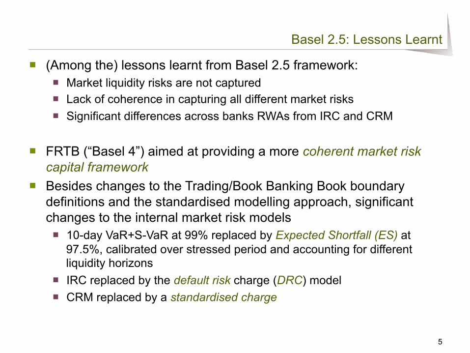
■  (Among the) lessons learnt from Basel 2.5 framework: ■  Market liquidity risks are not captured ■  Lack of coherence in capturing all different market risks ■  Significant differences across banks RWAs from IRC and CRM

■  FRTB (“Basel 4”) aimed at providing a more coherent market risk capital framework

■  Besides changes to the Trading/Book Banking Book boundary definitions and the standardised modelling approach, significant changes to the internal market risk models ■  10-day VaR+S-VaR at 99% replaced by Expected Shortfall (ES) at

97.5%, calibrated over stressed period and accounting for different liquidity horizons

■  IRC replaced by the default risk charge (DRC) model ■  CRM replaced by a standardised charge

5

Basel 2.5: Lessons Learnt

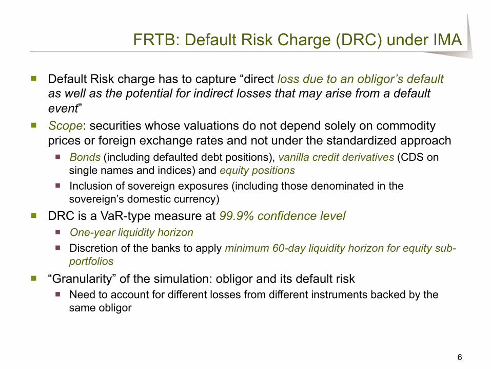
■  Default Risk charge has to capture “direct loss due to an obligor’s default as well as the potential for indirect losses that may arise from a default event”

■  Scope: securities whose valuations do not depend solely on commodity prices or foreign exchange rates and not under the standardized approach ■  Bonds (including defaulted debt positions), vanilla credit derivatives (CDS on

single names and indices) and equity positions ■  Inclusion of sovereign exposures (including those denominated in the

sovereign’s domestic currency) ■  DRC is a VaR-type measure at 99.9% confidence level

■  One-year liquidity horizon ■  Discretion of the banks to apply minimum 60-day liquidity horizon for equity sub-

portfolios ■  “Granularity” of the simulation: obligor and its default risk

■  Need to account for different losses from different instruments backed by the same obligor

6

FRTB: Default Risk Charge (DRC) under IMA

7

DRC Modelling

■  Standards for Minimum Capital Requirements for Market Risk published in Jan-2016

■  Regulatory requirements for the internal modelling in DRC tend to be more prescriptive than in the past

■  However the regulation still leaves some questions unanswered:

■  How to model and estimate default correlations under the new framework?

■  How to model loss given defaults (LGD)?

■  Two papers in the literature addressing these questions ■  Laurent et al. (2015) ■  Wilkens and Predescu (2016)

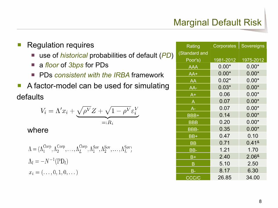
■  Regulation requires ■  use of historical probabilities of default (PD) ■  a floor of 3bps for PDs ■  PDs consistent with the IRBA framework

■  A factor-model can be used for simulating defaults

where

8

Marginal Default Risk

Rating (Standard and

Poor's)

Corporates Sovereigns

1981-2012 1975-2012 AAA 0.00* 0.00* AA+ 0.00* 0.00* AA 0.02* 0.00* AA- 0.03* 0.00* A+ 0.06 0.00* A 0.07 0.00* A- 0.07 0.00*

BBB+ 0.14 0.00* BBB 0.20 0.00* BBB- 0.35 0.00* BB+ 0.47 0.10 BB 0.71 0.41& BB- 1.21 1.70 B+ 2.40 2.06& B 5.10 2.50 B- 8.17 6.30

CCC/C 26.85 34.00

■  Regulation requires ■  default simulation model with two types of systematic risk factors ■  correlations based on listed equity prices or CDS spreads ■  correlations must be based on data covering a period of 10-years that

includes a period of stress and be based on a one-year liquidity horizon ■  Equity (and CDS) prices embed much more co-dependence than

the simple “default correlation” ■  Moody’s (2008): asset correlations used as predictors of default

correlations; ■  Düllmann et al. (2008): equity correlations overestimate asset

correlations; De Servigny and Renault (2002) and Qi et al. (2015): equity correlations are noisy indicators of default correlations

■  Nevertheless regulation points towards the use of a direct measure of correlation ■  Significant advantage for portfolio risk measurement, management and

analysis

9

Correlation of Defaults Across Obligors

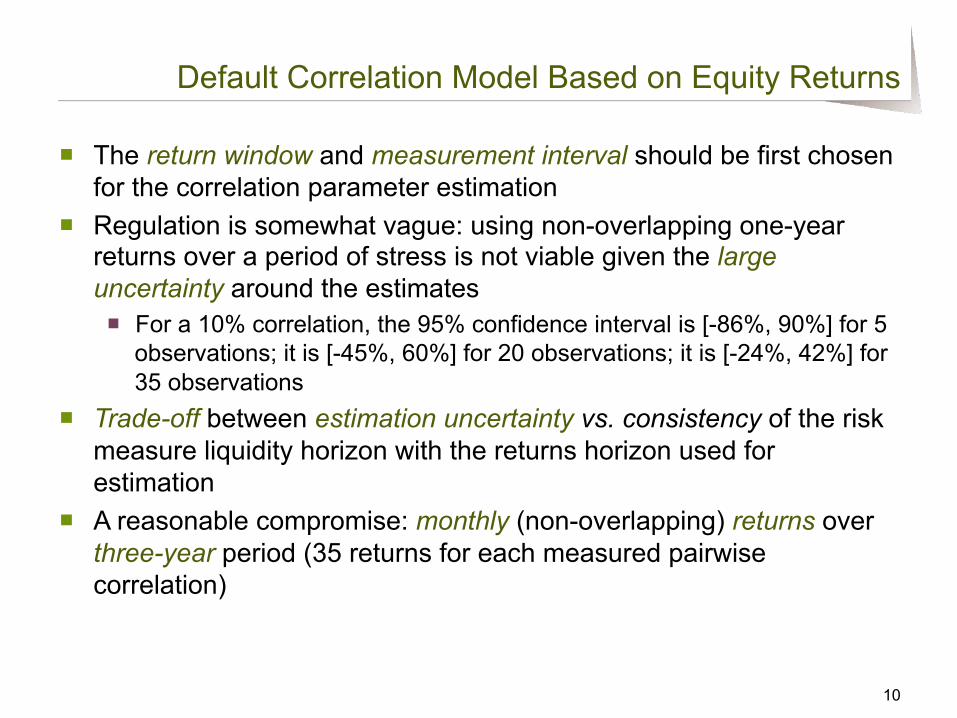
■  The return window and measurement interval should be first chosen for the correlation parameter estimation

■  Regulation is somewhat vague: using non-overlapping one-year returns over a period of stress is not viable given the large uncertainty around the estimates ■  For a 10% correlation, the 95% confidence interval is [-86%, 90%] for 5

observations; it is [-45%, 60%] for 20 observations; it is [-24%, 42%] for 35 observations

■  Trade-off between estimation uncertainty vs. consistency of the risk measure liquidity horizon with the returns horizon used for estimation

■  A reasonable compromise: monthly (non-overlapping) returns over three-year period (35 returns for each measured pairwise correlation)

10

Default Correlation Model Based on Equity Returns

11

Equity Returns Correlations over Time

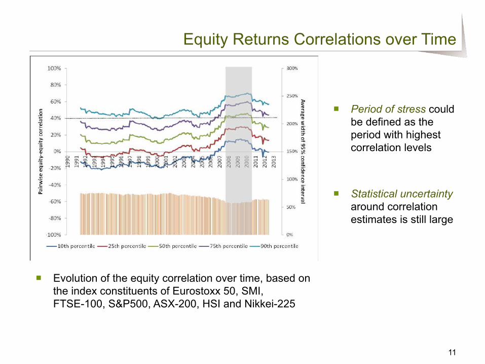
■  Evolution of the equity correlation over time, based on the index constituents of Eurostoxx 50, SMI, FTSE-100, S&P500, ASX-200, HSI and Nikkei-225

■  Statistical uncertainty around correlation estimates is still large

■  Period of stress could be defined as the period with highest correlation levels

12

Distribution of Correlations During The Stress Period

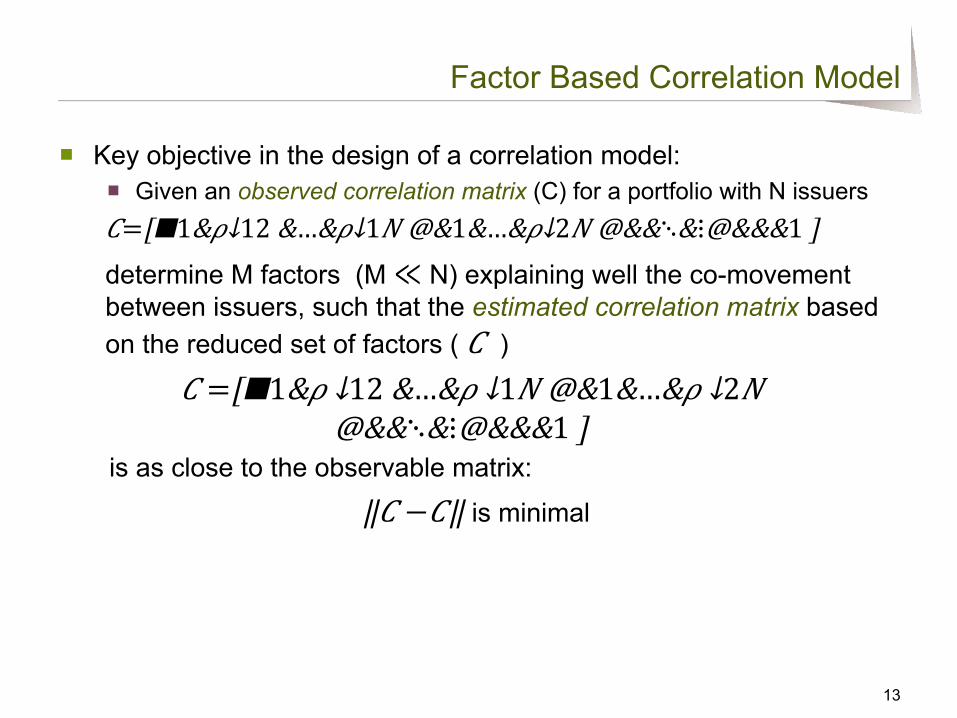
■  Key objective in the design of a correlation model: ■  Given an observed correlation matrix (C) for a portfolio with N issuers 𝐶=[█■1&𝜌↓12 &…&𝜌↓1𝑁 @&1&…&𝜌↓2𝑁 @&&⋱&⋮@&&&1 ] determine M factors (M ≪ N) explaining well the co-movement between issuers, such that the estimated correlation matrix based on the reduced set of factors ( 𝐶  )

𝐶 =[█■1&𝜌 ↓12 &…&𝜌 ↓1𝑁 @&1&…&𝜌 ↓2𝑁 @&&⋱&⋮@&&&1 ]

is as close to the observable matrix:

‖𝐶 −𝐶‖ is minimal

13

Factor Based Correlation Model

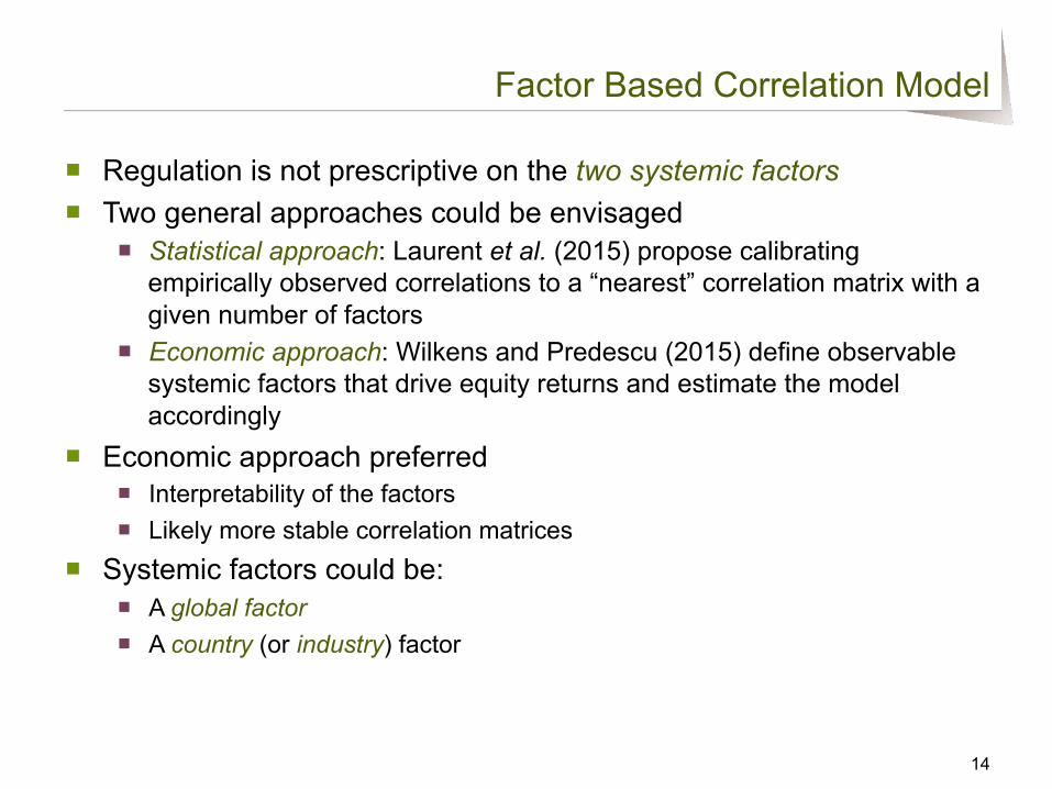
■  Regulation is not prescriptive on the two systemic factors ■  Two general approaches could be envisaged

■  Statistical approach: Laurent et al. (2015) propose calibrating empirically observed correlations to a “nearest” correlation matrix with a given number of factors

■  Economic approach: Wilkens and Predescu (2015) define observable systemic factors that drive equity returns and estimate the model accordingly

■  Economic approach preferred ■  Interpretability of the factors ■  Likely more stable correlation matrices

■  Systemic factors could be: ■  A global factor ■  A country (or industry) factor

14

Factor Based Correlation Model

■  Equity monthly non-overlapping returns time series are constructed from a large dataset of equity prices ■  1145 equities covering major equity indices (Eurostoxx 50, SMI,

FTSE-100, S&P500, ASX-200, HSI and Nikkei-2250)

■  Estimation approach ■  Construct standardized equity returns time series ( ) ■  Derive global ( ), country ( ) and industry ( ) returns at

each time point from the relevant cross-section of corporate returns

■  Dependence of country- or industry- factors on the global factor estimated via linear regressions

15

Equity Return Factor Model Estimation

16

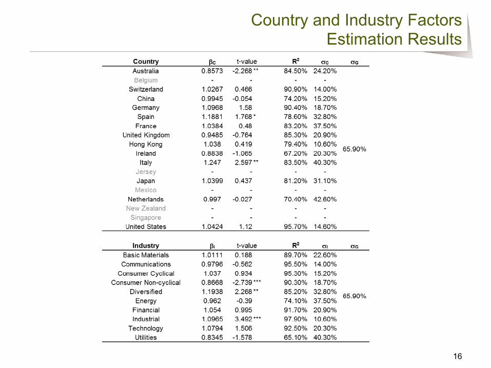
Country and Industry Factors Estimation Results

■  Linear dependence of individual equity returns on the systemic factors is estimated using panel regressions

■  Individual equity returns depend on the global factor and country specific and/or industry specific factors

17

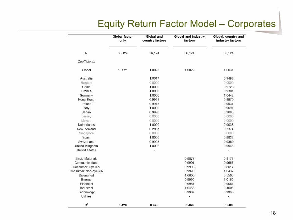
Equity Return Factor Model – Corporates

18

Equity Return Factor Model – Corporates

19

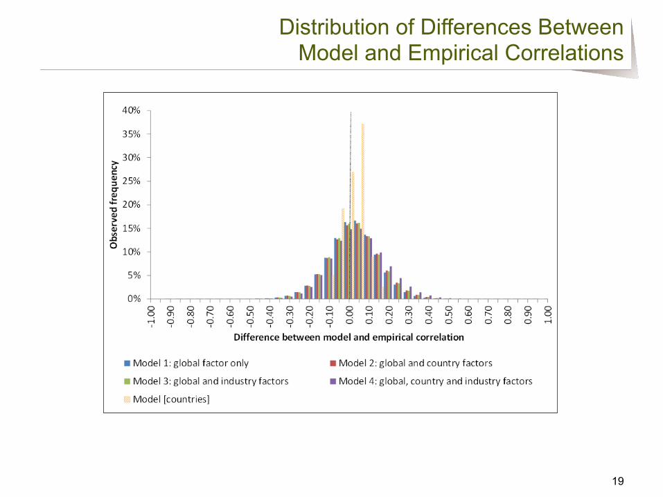
Distribution of Differences Between Model and Empirical Correlations

■  Regulation requires ■  dependence of recovery rates on the systemic risk factors ■  LGD estimates used as part of the IRBA approach for institutions with

such approved model ■  recovery rate of 0% for equities

■  Different approaches in the literature ■  Estimation of a linear inverse relation between historical average

recoveries and annual default rates (Altman et al. (2005)) ■  Recovery rate is linked to a systemic global factor and is assumed to

have a certain distribution ■  beta distribution - Moody’s (2005) and RiskMetrics Group (2007) ■  log-normal (Bade et al. (2011a, 2011b) ■  logit (Wilkens et al. (2013) ■  Vasicek-type distribution (Frye (2014))

20

Recovery Rate Risk

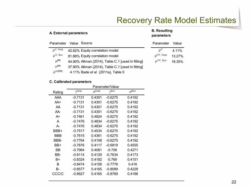
■  A log-normal recovery rate model similar to the one proposed in Bade et al. (2011a, 2011b) and based on previous work by Pykhtin (2003) is adopted

■  Log-recovery rate is assumed to be driven by a systemic factor and a purely idiosyncratic recovery rate component

■  The indicator vectors differentiate between rating categories

■  The deterministic vectors γ and σ reflect calibration parameters for corporates and sovereigns across different ratings

■  The estimate for is based on the Bade et al. (2011a) paper ■  The other parameters are estimated by fitting the first two moments

of the empirical distribution of recovery rates conditional on default

21

Recovery Rate Model

22

Recovery Rate Model Estimates

Parameter Value Parameter Value

ρV, Corp 42.82% ρY 4.11%ρV, Sov 81.88% ρVY, Corp 13.27%µRR 44.90% ρVY, Sov 18.35%σRR 37.90%ρ ln(RR) 4.11%

Rating σCorp γSov σSov

AAA 0.4301 -0.6275 0.4192AA+ 0.4301 -0.6275 0.4192AA 0.4301 -0.6275 0.4192AA- 0.4301 -0.6275 0.4192A+ 0.4824 -0.6275 0.4192A 0.4834 -0.6275 0.4192A- 0.4834 -0.6275 0.4192

BBB+ 0.4534 -0.6275 0.4192BBB 0.4361 -0.6275 0.4192BBB- 0.4108 -0.6275 0.4192BB+ 0.4117 -0.6819 0.4555BB 0.4081 -0.708 0.4271BB- 0.4129 -0.7634 0.4173B+ 0.4182 -0.769 0.4151B 0.4158 -0.7778 0.416B- 0.4165 -0.8099 0.4229

CCC/C 0.4165 -0.8769 0.4188

-0.8324-0.8474-0.8577-0.8927

-0.7517-0.7615-0.7764-0.7876-0.7964-0.8114

-0.7131-0.7131-0.7131-0.7461-0.7476-0.7476

C. Calibrated parametersParameter/Value

γCorp

-0.7131

Equity correlation modelAltman (2014), Table C.1 [used in fitting]Altman (2014), Table C.1 [used in fitting]Bade et al. (2011a), Table 5

A. External parameters B. Resulting parameters

Source

Equity correlation model

23

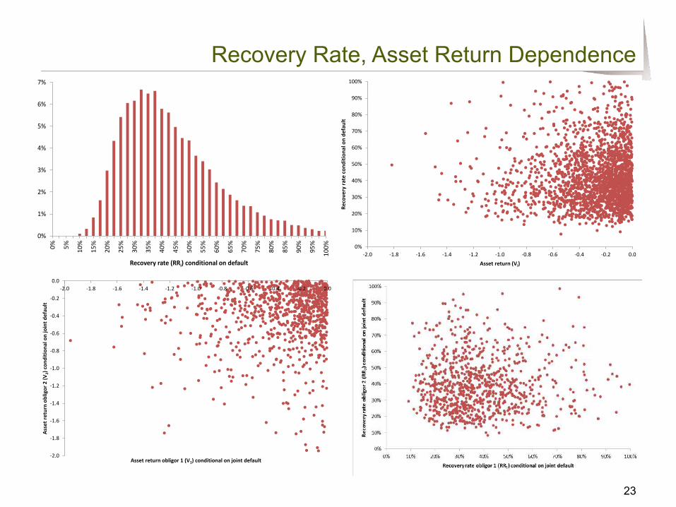
Recovery Rate, Asset Return Dependence

0%

1%

2%

3%

4%

5%

6%

7%

0% 5% 10%

15%

20%

25%

30%

35%

40%

45%

50%

55%

60%

65%

70%

75%

80%

85%

90%

95%

100%

Recovery  rate  (RRi)  conditional  on  default

0%

10%

20%

30%

40%

50%

60%

70%

80%

90%

100%

-­‐2.0 -­‐1.8 -­‐1.6 -­‐1.4 -­‐1.2 -­‐1.0 -­‐0.8 -­‐0.6 -­‐0.4 -­‐0.2 0.0

Recovery  ra

te  con

ditio

nal  on  de

fault

Asset  return  (Vi)

-­‐2.0

-­‐1.8

-­‐1.6

-­‐1.4

-­‐1.2

-­‐1.0

-­‐0.8

-­‐0.6

-­‐0.4

-­‐0.2

0.0-­‐2.0 -­‐1.8 -­‐1.6 -­‐1.4 -­‐1.2 -­‐1.0 -­‐0.8 -­‐0.6 -­‐0.4 -­‐0.2 0.0

Asset  return  ob

ligor  2  (V

2)  con

ditio

nal  on  joint  d

efau

lt

Asset  return  obligor  1  (V1)  conditional  on  joint  default

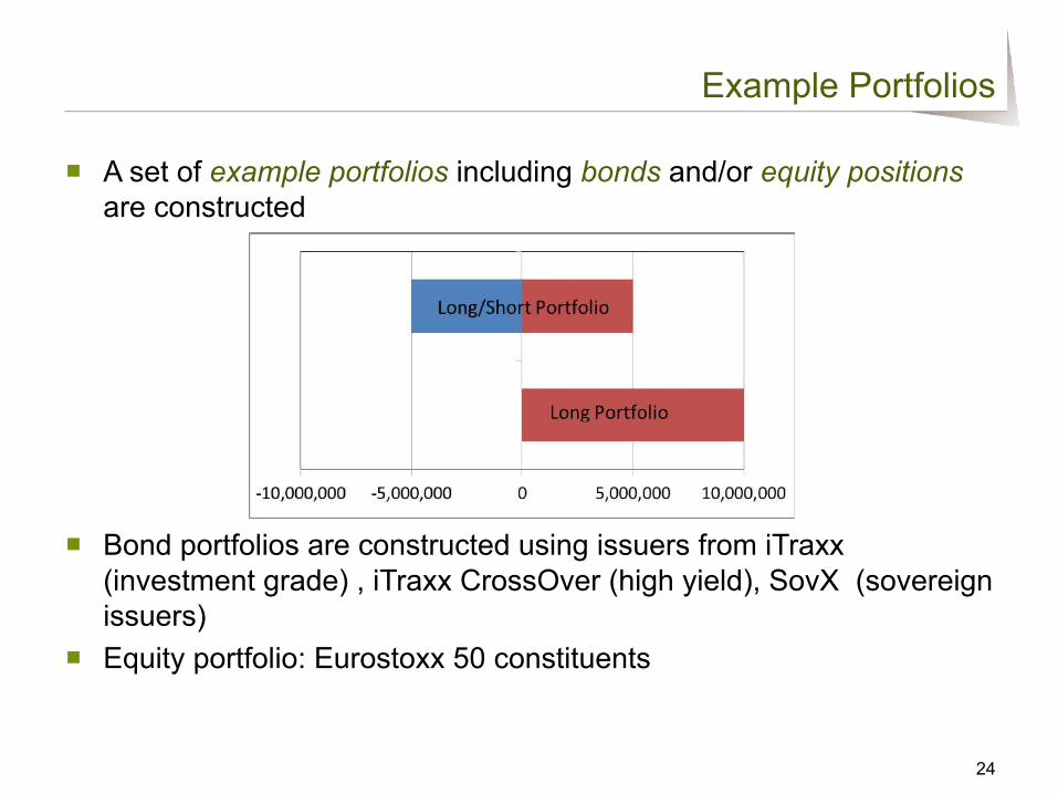
■  A set of example portfolios including bonds and/or equity positions are constructed

■  Bond portfolios are constructed using issuers from iTraxx (investment grade) , iTraxx CrossOver (high yield), SovX (sovereign issuers)

■  Equity portfolio: Eurostoxx 50 constituents

24

Example Portfolios

25

P&L distributions and DRC figures

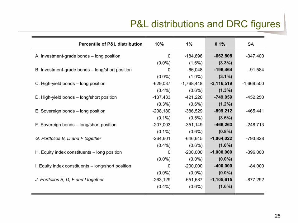
Percentile of P&L distribution 10% 1% 0.1% SA A. Investment-grade bonds – long position 0 -184,696 -662,808 -347,400

(0.0%) (1.6%) (3.3%) B. Investment-grade bonds – long/short position 0 -66,048 -196,464 -91,584

(0.0%) (1.0%) (3.1%) C. High-yield bonds – long position -629,037 -1,768,448 -3,116,519 -1,669,500

(0.4%) (0.6%) (1.3%) D. High-yield bonds – long/short position -137,433 -421,220 -749,059 -452,250

(0.3%) (0.6%) (1.2%) E. Sovereign bonds – long position -208,180 -386,529 -899,212 -465,441

(0.1%) (0.5%) (3.6%) F. Sovereign bonds – long/short position -207,003 -351,149 -466,263 -248,713

(0.1%) (0.6%) (0.8%) G. Portfolios B, D and F together -264,601 -646,645 -1,064,022 -793,828

(0.4%) (0.6%) (1.0%) H. Equity index constituents – long position 0 -200,000 -1,000,000 -396,000

(0.0%) (0.0%) (0.0%) I. Equity index constituents – long/short position 0 -200,000 -400,000 -84,000

(0.0%) (0.0%) (0.0%) J. Portfolios B, D, F and I together -263,129 -651,687 -1,105,615 -877,292

(0.4%) (0.6%) (1.6%)

26

Comparison to the Standardised Approach for DRC

■  Figures show Model-based DRC vs Standardised Approach (SA) -based DRC for an equity portfolio of BBB-rated obligors. (Nominal for each position =1, LGD=100%)

■  Difference between the Model-based and SA-based DRC depends on: ■  Returns Correlation in the model-based framework ■  Portfolio Size ■  Ratio of Long Jump-to-Default to total Jump-to-Default ■  Marginal PDs and LGDs in the model-based framework

27

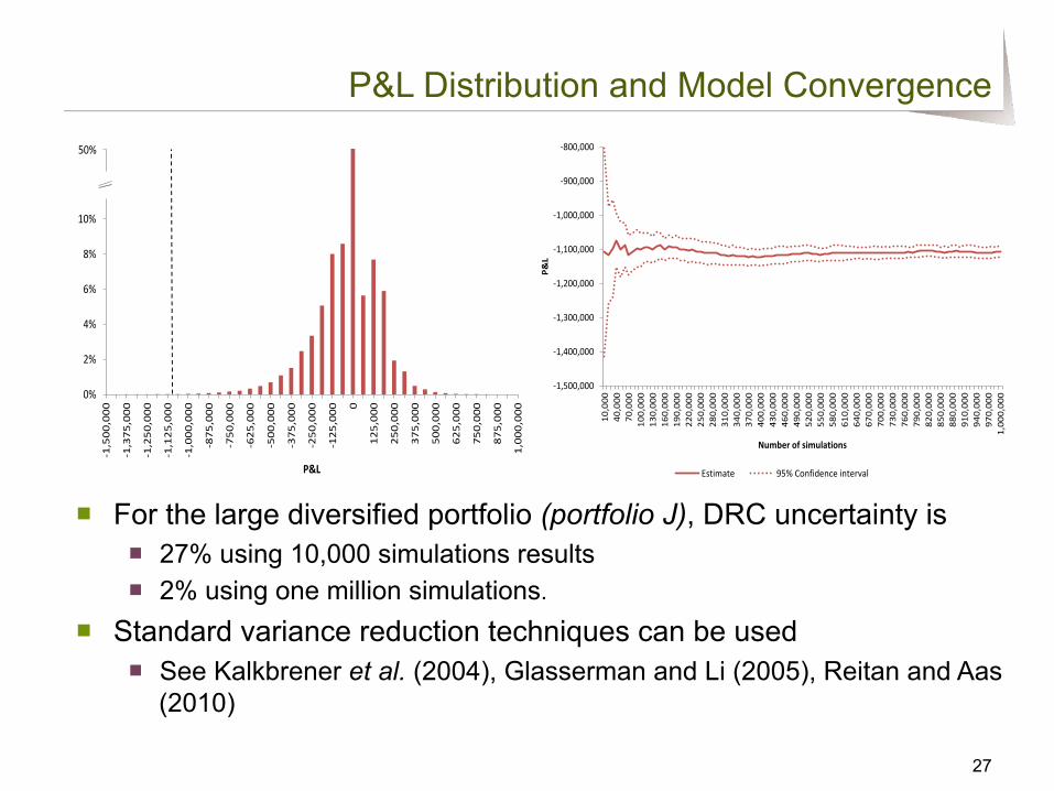
P&L Distribution and Model Convergence

0%

2%

4%

6%

8%

10%

12%

14%

-­‐1,500,000

-­‐1,375,000

-­‐1,250,000

-­‐1,125,000

-­‐1,000,000

-­‐875

,000

-­‐750

,000

-­‐625

,000

-­‐500

,000

-­‐375

,000

-­‐250

,000

-­‐125

,000 0

125,000

250,000

375,000

500,000

625,000

750,000

875,000

1,000,000

P&L

50%

-­‐1,500,000

-­‐1,400,000

-­‐1,300,000

-­‐1,200,000

-­‐1,100,000

-­‐1,000,000

-­‐900,000

-­‐800,000

10,000

40,000

70,000

100,00

013

0,00

016

0,00

019

0,00

022

0,00

025

0,00

028

0,00

031

0,00

034

0,00

037

0,00

040

0,00

043

0,00

046

0,00

049

0,00

052

0,00

055

0,00

058

0,00

061

0,00

064

0,00

067

0,00

070

0,00

073

0,00

076

0,00

079

0,00

082

0,00

085

0,000

880,00

091

0,000

940,00

097

0,00

01,00

0,00

0

P&L

Number  of  simulations

Estimate 95%  Confidence  interval

■  For the large diversified portfolio (portfolio J), DRC uncertainty is ■  27% using 10,000 simulations results ■  2% using one million simulations.

■  Standard variance reduction techniques can be used ■  See Kalkbrener et al. (2004), Glasserman and Li (2005), Reitan and Aas

(2010)

28

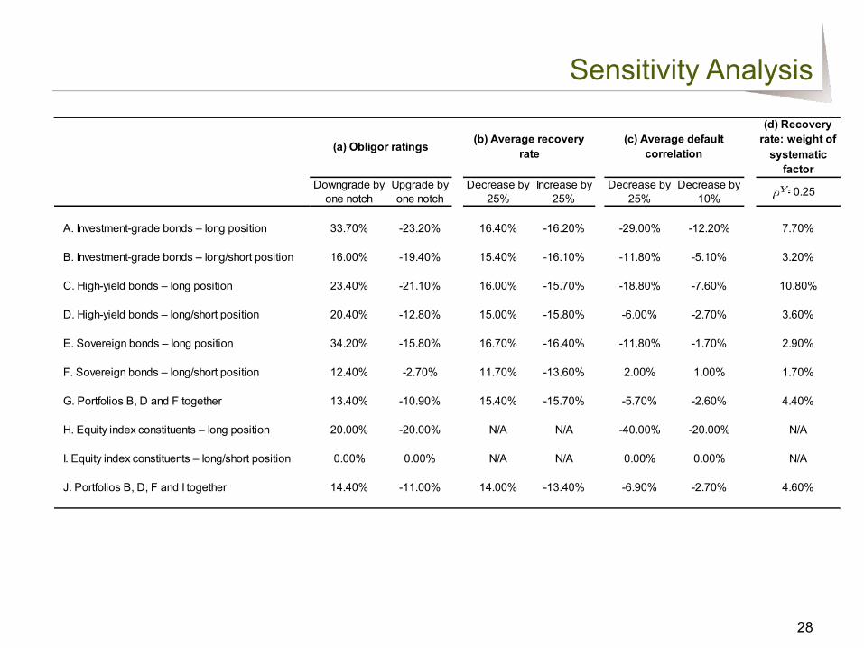
Sensitivity Analysis

(d) Recovery rate: weight of

systematic factor

Downgrade by Upgrade by Decrease by Increase by Decrease by Decrease byone notch one notch 25% 25% 25% 10%

A. Investment-grade bonds – long position 33.70% -23.20% 16.40% -16.20% -29.00% -12.20% 7.70%

B. Investment-grade bonds – long/short position 16.00% -19.40% 15.40% -16.10% -11.80% -5.10% 3.20%

C. High-yield bonds – long position 23.40% -21.10% 16.00% -15.70% -18.80% -7.60% 10.80%

D. High-yield bonds – long/short position 20.40% -12.80% 15.00% -15.80% -6.00% -2.70% 3.60%

E. Sovereign bonds – long position 34.20% -15.80% 16.70% -16.40% -11.80% -1.70% 2.90%

F. Sovereign bonds – long/short position 12.40% -2.70% 11.70% -13.60% 2.00% 1.00% 1.70%

G. Portfolios B, D and F together 13.40% -10.90% 15.40% -15.70% -5.70% -2.60% 4.40%

H. Equity index constituents – long position 20.00% -20.00% N/A N/A -40.00% -20.00% N/A

I. Equity index constituents – long/short position 0.00% 0.00% N/A N/A 0.00% 0.00% N/A

J. Portfolios B, D, F and I together 14.40% -11.00% 14.00% -13.40% -6.90% -2.70% 4.60%

= 0.25

(a) Obligor ratings (b) Average recovery rate

(c) Average default correlation

■  The new default risk charge should capture the risk arising from long/short positions from the timing of defaults within a one-year capital horizon ■  For example a long 1-year bond position hedged with a 3-month

CDS should take into account loss scenarios generated by the issuer defaulting between months four and twelve

■  Multi-step model allows for a consistent default risk simulation for obligors with equity and credit instruments attracting different liquidity horizons ■  For example the default probability for the credit instrument over

the first 60 days should be the same as for the equity instrument (with a 60-day liquidity horizon) given the same underlying obligor.

29

Multiple Time Horizons in DRC

■  A multi-step default model needed ■  Modelling the probability of default over the different sub-

periods ■ See Smillie and Epperlein (2007)

■  Modelling of default correlation over sub-periods ■ The “correlation wash-out” phenomenon (correlation

break-down generated by increasing sampling time steps) should be addressed

■ See Dunn (2008)

30

Multiple Time Horizons Modelling

■  FRTB is a major overhaul of the current market risk framework

■  Although targeted for 2019, banks will likely need to make significant changes to their internal market risk models

■  Wilkens and Predescu (2016) presents one comprehensive DRC model compliant with the current FRTB regulatory text

■  Potential future analyses: ■ Model risk (see e.g. Glasserman and Xu (2014)) ■ Variance reduction techniques and EVT ■ Default Risk portfolio risk analysis: risk drivers and

associated contributions 31

Concluding Remarks

■  Wilkens and Predescu (2016), “Default Risk Charge (DRC): Modeling Framework for the 'Basel 4' Risk Measure”

http://papers.ssrn.com/sol3/papers.cfm?abstract_id=2638415

32

Main Reference