Fundamental process design principles for the OBM ... · PDF fileFundamental process design...

Fundamental process design principles for the OBM, including cost assessment

Techneau, 06. January 2008

© 2006 TECHNEAU TECHNEAU is an Integrated Project Funded by the European Commission under the Sixth Framework Programme, Sustainable Development, Global Change and Ecosystems Thematic Priority Area (contractnumber 018320). All rights reserved. No part of this book may be reproduced, stored in a database or retrieval system, or published, in any form or in any way, electronically, mechanically, by print, photoprint, microfilm or any other means without prior written permission from the publisher

Fundamental process design principles for the OBM, including cost assessment

Techneau, 06. January 2008

Colofon

Title Fundamental process design principles for the OBM, including cost assessment Author(s) Kamal Azrague and Stein W. Osterhus Quality Assurance Stein W. Osterhus and Kamal Azrague Deliverable number D 2.2.1.

This report is: PU

Contents

Contents 1

1 Introduction and description of the OBM process 2

2 Design principles 4

2.1 Oxidation 4 2.1.1General 4 2.1.2Design configuration of ozonation systems 4

2.1.2.1Gas feed systems 5 2.1.2.2Ozone generators 7 2.1.2.3Ozone contactors 11 2.1.2.4Off-gas destruction Systems 14

2.1.3Ozone system design principles 15 2.1.3.1Color removal from NOM containing water 15 2.1.3.2Oxidation of inorganic and organic compounds 16 2.1.3.3Hygenic barrier and disinfection 19

2.1.4Factors affecting the ozone system design 21 2.1.5Alternative and additional oxidation methods 22

2.2 Biodegradation 22 2.2.1Biofilter design 23 2.2.2Filter media in biofilters 25

2.3 Membrane filtration 26 2.3.1Membrane design characteristics 27

2.3.1.1Types of UF/MF membrane systems 27 2.3.1.2Membrane material properties 29 2.3.1.3Performance characteristics 31

2.3.2Design of the membrane filtration plant after the oxidation-biofiltration 33 2.3.2.1Choice of the membrane 33 2.3.2.2Design of the plant 33

3 Preliminary cost assessment 36

3.1 Ozonation 36 3.1.1Capital cost 36 3.1.2O&M cost 37

3.2 Biofiltration 38

3.3 Membrane filtration 38 3.3.1Capital cost 38 3.3.2O&M cost 39

3.4 Total cost Estimate of the OBM 39

TECHNEAU Kamal Azrague and Stein W. Osterhus © TECHNEAU - 1 -

1 Introduction and description of the OBM process

Modern drinking water treatment has to meet many requirements, including high removal efficiency of NOM, iron, manganese, ammonia and various organic micro pollutants, in addition to provide satisfactory hygienic barriers for pathogens. The need to find methods that provide effective treatment processes at low costs combining different steps, have lead to the use of the term “multi-barrier”. The desirable characteristics of such treatment methods include:

Removal of pollutants (NOM, organic trace pollutant, etc) Inactivation of pathogenic organisms Reduction in disinfection by-products

In order to meet these characteristics, treatment trains have been developed that improve both removal of pollutant and disinfection in multiple steps of the water treatment. For example, ozone may be added to perform preliminary disinfection and oxidation of inorganic and organic materials including micro-pollutants, coagulation and separation followed by sand filtration for removal of disinfection by-product precursors, and chlorine addition immediately before the distribution network so that a disinfectant residual may be maintained. Another common train for the disinfection of sand filtered effluent is to use ultraviolet light, followed by the addition of chlorine to maintain a residual. Others, on the other hand, avoid having a chlorine residual in the network. Not only does a multi-barrier approach allow several contaminants to be removed, but the total number of pathogens removed will be increased, which reduces the possibility of pathogen ingestion by water users. Multi-barrier techniques may be expected to become more prevalent in the future, and will need to be matched to the source water quality to effectively meet water treatment goals. Ozonation followed by biofiltration is a well known process combination, and is considered as one of the most promising processes in the advanced drinking water treatment (Malley et al. 1993). However, the biofiltration step will produce/release sludge, bacteria and particles which should be removed from the water before distribution. This could be achieved by for instance membrane filtration. Consequently a novel process combination consisting of the three steps oxidation (ozonation), biodegradation and micro or ultra membrane filtration (OBM) is being developed (figure 1). The OBM process belong to the “multi-barrier” concept and it can be characterize as a strongly robust process since it comprises of an oxidation step (e.g. ozonation) which is known to be very efficient towards pollutants and pathogens, and a membrane filtration step which, depending on the pore size, remove bacteria, parasites and in the case of certain ultrafiltration membranes, also viruses. This makes the OBM a promising system which can meet required drinking water qualities.



In the present report the design principles and a cost assessment of the OBM process have been presented. Depending on the water quality, different recommendations will be given for the design of such process, and a preliminary assessment of the cost of this system will be presented for two treatment plants with a capacity of 20000 m3/day and 3600 m3/day, respectively.

Figure 1 Schematic sketch of the OBM process.

Chemicaloxidation• O3

• UV/H2O2• UV/TiO2

Biologicaloxidation• Biofilm reactor• Susp. biomass

Membranefiltration• Nanofiltration• Ultrafiltration• Microfiltration

Chemical degradation of:• Trace organics (NDMA, MTBE, ED)• NOM (color removal)• Taste and odor (MIB, Geosmin etc)• Oxidation of inorganics (Fe, Mn)Disinfection (1. barrier)

Biological degradation of organicchemical oxidation byproducts:• Trace organics residuals• NOM (aldehydes, ketones, etc)• Taste and odor residuals

Membrane separation of : • Inorganic trace pollutants• Biomass produced upstream• Oxidized/precipitated inorganics• Pathogens (2. barrier)

Chemicaloxidation• O3

• UV/H2O2• UV/TiO2

Biologicaloxidation• Biofilm reactor• Susp. biomass

Membranefiltration• Nanofiltration• Ultrafiltration• Microfiltration

Chemical degradation of:• Trace organics (NDMA, MTBE, ED)• NOM (color removal)• Taste and odor (MIB, Geosmin etc)• Oxidation of inorganics (Fe, Mn)Disinfection (1. barrier)

Biological degradation of organicchemical oxidation byproducts:• Trace organics residuals• NOM (aldehydes, ketones, etc)• Taste and odor residuals

Membrane separation of : • Inorganic trace pollutants• Biomass produced upstream• Oxidized/precipitated inorganics• Pathogens (2. barrier)

2 Design principles

2.1 Oxidation

2.1.1 General The purpose of the oxidation step could be very many, including:

To remove or reduce the concentration of harmful or undesirable compounds by oxidation.

o Remove color from NOM containing water o Remove taste and odor o Oxidize soluble inorganic compounds to compounds off less

concern o Completely mineralize persistent organic compounds and

micro pollutants, or partly oxidize them to compounds of less concern

Oxidative conversion of harmful or undesirable compounds to more easily removable compounds.

o Oxidize soluble inorganic compounds (i.e. Fe2+, Mn2+) to less soluble compounds that will precipitate and removed later in the process.

o Partly oxidize NOM to easy biodegradable organics o Oxidize persistent organic compounds and micro pollutants to

easy biodegradable compounds Provide hygienic barrier towards pathogens.

o Pre-disinfection Oxidation by ozone will be the reference method of oxidation, and the method that will be considered in this report. However, several other oxidation methods and combinations are also possible. They will only be mentioned in this report, but will be considered in more detail at a later stage.

2.1.2 Design configuration of ozonation systems As shown in Figure 2, ozone water treatment systems have four basic components: a gas feed system, an ozone generator, an ozone contactor, and an off-gas destruction system. The gas feed system provides a clean, dry source of air or oxygen to the generator. The ozone contactor transfers the ozone-rich gas into the water to be treated, and provides contact time for disinfection or other reactions. Consequently, the ozone contactor can be further divided into a transfer component and a reaction component, although they are often not easy to distinguish. The final process step, off-gas destruction, is required as ozone is toxic in the concentrations present in the off-gas.


Figure 2. Simplified schematic of the primary components of an ozone process.

2.1.2.1 Gas feed systems Ozone feed systems are classified as using air, high purity oxygen or mixture of the two. High purity oxygen can be purchased and stored as a liquid (LOX), or it can be generated on-site through either a cryogenic process, with vacuum swing adsorption (VSA), or with pressure swing adsorption (PSA). Cryogenic generation of oxygen is a complicated process and is feasible only in large systems. Pressure swing adsorption is a process whereby a special molecular sieve is used under pressure to selectively remove nitrogen, carbon dioxide, water vapor, and hydrocarbons from air, producing an oxygen rich (80–95 percent O2) feed gas. The components used in pressure swing adsorption systems are similar to high pressure air feed systems in that both use pressure swing molecular absorption equipment. Low pressure air feed systems use a heat reactivated desiccant dryer. Oxygen Feed Systems - Liquid oxygen feed systems are relatively simple, consisting of a storage tank or tanks, evaporators to convert the liquid to a gas, filters to remove impurities, and pressure regulators to limit the gas pressure to the ozone generators. Air Feed Systems - Air feed systems for ozone generators are fairly complicated as the air should be properly conditioned to prevent damage to the generator. Air should be clean and dry, with a maximum dew point of -


60º C (-80º F) and free of contaminants. Air preparation systems typically consist of air compressors, filters, dryers, and pressure regulators. Table 1 presents a comparison of the advantages and disadvantages of each gas feed system. Particles greater than 1 mm and oil droplets greater than 0.05 mm should be removed by filtration (Langlais et al. 1991). If hydrocarbons are present in the feed gas, granular activated carbon filters should follow the particulate and oil filters. Moisture removal can be achieved by either compression or cooling (for large-scale system), which lowers the holding capacity of the air, and by desiccant drying, which strips the moisture from the air with a special medium. Desiccant dryers are required for all air preparation systems. Large or small particles and moisture cause arcing which damages generator dielectrics. Typically, desiccant dryers are supplied with dual towers to allow regeneration of the saturated tower while the other is in service. Moisture is removed from the dryer by either an external heat source or by passing a fraction (10 to 30 percent) of the dried air through the saturated tower at reduced pressure. Formerly, small systems that require only intermittent use of ozone, a single desiccant tower is sufficient, provided that it is sized for regeneration during ozone decomposition time. Table 1. Comparison of air and high purity oxygen feed systems.

Air preparation systems can be classified by the operating pressure: ambient, low (less than 30 psig), medium, and high (greater than 60 psig) pressure. The distinguishing feature between low and high pressure systems is that high pressure systems can use a heatless dryer. A heatless dryer operates normally in the 100 psig range, rather than the 60 psig range. Rotary lobe, centrifugal,


rotary screw, liquid ring, vane, and reciprocating compressors can be used in air preparation systems. Table 2 lists the characteristics of many of these types of compressors. Reciprocating and liquid ring compressors are the most common type used in the United States, particularly in small systems, the former because the technology is so prevalent and the latter because liquid ring compressors do not need aftercoolers. Air receivers are commonly used to provide variable air flow from constant volume compressors. Oil-less compressors are used in modern systems to avoid hydrocarbons in the feed gas (Dimitriou, 1990). Table 2. Types of compressors used in air preparation systems.

2.1.2.2 Ozone generators Ozone can be produced several ways, although one method, corona discharge, predominates in the ozone generation industry. Ozone can also be produced by irradiating an oxygen-containing gas with ultraviolet light, electrolytic reaction and other emerging technologies as described by Rice (Rice 1996). Corona discharge, also known as silent electrical discharge, consists of passing an oxygen-containing gas through two electrodes separated by a dielectric and a discharge gap. Voltage is applied to the electrodes, causing an electron flow through across the discharge gap. These electrons provide the energy to disassociate the oxygen molecules, leading to the formation of ozone. Figure 3 shows a basic ozone generator.


Figure 3. Basic ozone generator. Ozone generator efficiency - Theoretically, ozone generation should yield an energy efficiency of 400 g/kWh (grams of ozone formed per hour, per kW of power input) in oxygen. Current ozone generators reach efficiencies of about 120 g/kWh. It is clear that ozone generation, even at the theoretical optimum value, is very energy inefficient. This is because almost 66 % of the input energy is converted to heat, which has to be removed from the ozone generator. Discharge physics provide a number of parameters to control the efficiency of ozone generation:

The value of the voltage peak (Vp) determines the applied electric field and therefore controls the energy of the electrons. An optimum peak voltage range exists.

The frequency of the applied voltage wave determines the concentration of micro discharges, and therefore controls the number density of the electrons, and the rate of oxygen dissociation. Higher frequency implies higher ozone generation, but also an increase in heat dissipation. Table 3 show a comparison between low, medium, and high frequency generators.

The air gap also determines the applied field, as well as the efficiency of cooling.

The dielectric barrier thickness and its value of dielectric constant controls the applied field, determines value of corona onset (Vc) and limits the amount of energy that can be deposited in the air gap in the form of micro-discharges.

The gas pressure determines the energy of the free electrons, as well as the concentration of oxygen molecules. It also determines the energy of ions in the discharge, which causes heat formation, and inefficient use of input energy.


Ozone generator design involves optimisation of these interrelated parameters with specific objectives in mind. Table 3. Comparison of low, medium, and high frequency ozone generators.

Volume discharge generators - The form of ozone generator shown in Figure 3 is known as a volume discharge generator. The dielectric barrier is intimately joined to the high-voltage electrode. An air gap separates the dielectric from the grounded electrode. Air or oxygen flows through the volume of this gap, where the micro-discharge cold plasma columns generate ozone. Gap distances vary between 0.5 and 3 mm, large gaps requiring higher voltage levels to operate. Water, oil, or air flowing across the outer surface cools the grounded wall of the generator. Sometimes the inner electrode is also cooled. Conventional ozone generators are built to the volume discharge configuration. In practice, the electrodes can be tubes (Wellsbach design) or plates (Lowther design). Considerable development and progress have been made in improving the generation efficiency of volume discharge ozone generators. The major thrust of most of the improvement lies in the dielectric barrier. Considering the effects mentioned above, two disadvantages of the volume discharge become apparent:

Heat is dissipated in the volume of the air gap, and is not efficiently transported to the cooled walls. It is difficult to properly cool volume discharges.


The gap is filled with micro-discharges. The air stream and diffusion processes transport ozone formed in the gap into these, where ozone molecules are destroyed.

Volume discharge requires relatively high voltage levels, adding to physical size and cost of power supply equipment.

Other disadvantages are more subtle, and relate to poor response to pressure increases, and a limited range of operational parameters (flexibility) (Masuda and Kiss 1986). Ozone yield of volume discharge ozone generators fed with oxygen is about two to three times higher than with air (Pietsch 1998). Surface discharge generators - Figure 4 shows another form of dielectric barrier discharge. The high-voltage electrode is a conductor in intimate contact with the dielectric layer. The conductor can be round or square in cross section. Corona discharge is initiated at the contact surface of the conductor and dielectric by a very specific mechanism (Kuffel and Zaengl 1992) different from volume discharge. This mechanism causes the corona onset voltage (Vc) to be much lower than for volume discharge, and high voltage levels as low as 1.5 kV may be used dependent on the layer thickness. Once initiated, micro discharge columns also extend from the conductor and spread over the surface of the dielectric. The discharge is in contact with the dielectric barrier. In practice, arrays of conductors are distributed across the surface of the dielectric in the form of strips on a flat dielectric, or wires wound around a tubular dielectric. The grounded electrode can be cooled as in volume discharge. The electrode structure is enclosed in a sheath, with air or oxygen flowing through the gap between the electrodes and the sheath. Ozone is formed in the micro discharges, and escapes into the flowing gas stream.

Figure 4. Surface discharge configuration. The low cost ozone generator provided by Chris Swartz Water Utilisatin Engineers which is being evaluated as part of the OBM process is a surface


discharge generator. The use of surface discharge in ozone generation is relatively new, and was pioneered by Masuda (Masuda and Kiss 1986; Masuda et al. 1986). The surface discharge has a number of advantages above the volume discharge configuration, which led to the choice of this configuration for the new development:

The discharge occurs on the surface of the dielectric. Heat formed in the discharge is therefore relatively easy to remove through the heat conducting dielectric layer. Better heat removal enables the use of higher frequency, and therefore higher power deposition in the reactor.

Ozone formed in the discharge diffuses to the discharge free zone above the discharge and cannot be destroyed in the corona.

By correct selection of dielectric material, a thin layer can be established. This allows considerable reduction in the high-voltage level required (e.g. 3 kV as opposed to 10 kV), and more compact power supply. It also allows the use of a much higher frequency of discharge (e.g. 20 kHz as opposed to 2 kHz and lower), again resulting in considerable size reductions, and higher power deposition.

More subtly, surface discharge allows a wide range of operational parameters to be optimised for given ozone generation requirements. E.g. the ozone concentration can be doubled by an increase in pressure from 101 to 150 kPa (Masuda and Kiss 1986). No such improvement is possible with conventional volume discharge.

Ozone formation in surface discharge is not as susceptible as volume discharge to moisture conditions in terms of reduction in concentration. Ozone production is reduced by only 30 % at a relative humidity of 95 % in surface discharge (Masuda and Kiss 1986).

Optimised surface discharge ozone generators can yield 5 times higher production rate with oxygen than with air (Pietsch 1998). Surface discharge ozone generators seem more susceptible to the effects of moisture than volume discharge, in terms of the corrosive effects of nitric acid formed in presence of moisture.

2.1.2.3 Ozone contactors Once ozone gas is transferred into water, the dissolved ozone reacts with the organic and inorganic constituents, including any pathogens. Ozone not transferred into the process water during contacting is released from the contactor as off-gas. Transfer efficiencies of greater than 80 percent typically are required for efficient ozone disinfection (DeMers and Renner 1992). Common ozone dissolution methods include: Bubble diffuser contactors; Injectors; and Turbine mixers.


Bubble diffuser contactor - This method offers the advantages of no additional energy requirements, high ozone transfer rates, process flexibility, operational simplicity, and no moving parts. Figure 5 illustrates a typical three stage ozone bubble diffuser contactor. This illustration shows a countercurrent flow configuration (ozone and water flowing in opposite directions), an alternating cocurrent/countercurrent arrangement, and a cocurrent flow configuration (ozone and water flowing in the same direction). Also, the number of stages can vary from two to six for ozone disinfection, with the majority of plants using two or three chambers for contacting and reaction (Langlais et al. 1991).

Figure 5. Ozone bubble contactors. Bubble diffuser contactors are typically constructed with 18 to 22 ft water depths to achieve 85 to 95 percent ozone transfer efficiency. Since all the ozone is not transferred into the water, the contactor chambers are covered to contain the off-gas. Off-gas is routed to an ozone destruct unit, usually catalysts, thermal, or thermal/catalysts.


Bubble diffuser contactors use ceramic or stainless steel diffusers that are either rod-type or disc-type to generate bubbles. Design considerations for these diffusers (Renner et al. 1988) include: Gas flow range of 0.5 to 4.0 scfm; Maximum headloss of 0.5 psig; Permeability of 2 to 15 cfm/ft2/in of diffuser thickness; and porosity of 35 to 45 percent. The configuration of the bubble diffuser contactor structure should best be designed to provide plug flow hydraulics. This configuration will minimize the overall volume and avoid short circuiting. Contactor volume is determined in conjunction with the applied ozone dosage and estimated residual ozone concentration to satisfy oxidation kinetics and the disinfection CT (concentration times hydraulic retention time) requirement. Also, diffuser pore clogging can be a problem when ozone dosages are intermittent and/ or when iron and manganese oxidation is required. Channeling of bubbles is dependent on the type of diffusers used and the spacing between diffusers. Injector dissolution - Ozone is injected into a water stream under negative pressure, which is generated in a venturi section, pulling the ozone into the water stream. In many cases, a sidestream of the total flow is pumped to a higher pressure to increase the available vacuum for ozone injection. After the ozone is injected into this sidestream, the sidestream containing all the added ozone is combined with the remainder of the plant flow under high turbulence to enhance dispersion of ozone into the water. Figure 6 illustrates typical in-line and sidestream ozone injection systems.

Figure 6. In-line and sidestream ozone injection systems. The gas to liquid ratio is a key parameter used in the design of injector contacting systems. This ratio should be less than 0.067 cfm/gpm to optimize ozone transfer efficiency (Langlais et al. 1991). Meeting this criterion typically requires relatively low ozone dosages and ozone gas concentrations greater than 6 percent by weight (DeMers and Renner 1992). High concentration


ozone gas can be generated using a medium-frequency generator and/or liquid oxygen as the feed gas. To meet the requirements for oxidation volume and/or CT disinfection, additional contact time is required after the injector, typically in a plug flow reactor. The additional contact volume is determined in conjunction with the applied ozone dosage and estimated residual ozone concentration to satisfy the oxidation kinetics and/or the disinfection CT requirement. Turbine mixer contactors - Turbine mixers are used to feed ozone gas into a contactor and mix the ozone with the water in the contactor. Figure 7 illustrates a typical turbine contactor. The illustrated turbine mixer design shows the motor located outside the basin, allowing for maintenance access. Other designs use a submerged turbine. Ozone transfer efficiency for turbine mixers can be in excess of 90 percent. However, the power required to achieve this efficiency is 2.2 to 2.7 kW-hr of energy per lb of ozone transferred (Dimitriou, 1990). Turbine mixing basins vary in water depth from 6 to 15 ft, and dispersion areas vary from 5 to 15 ft (Dimitriou 1990). Again, as with injector contacting, sufficient contact time may not be available in the turbine basin to meet the requirement for oxidation volume and/or disinfection CT; consequently additional contact volume may be required.

Figure 7. Turbin mixer ozone contactor.

2.1.2.4 Off-gas destruction Systems The concentration of ozone in the off-gas from a contactor is usually well above the fatal concentration. For example, at 90 percent transfer efficiency, a 3 percent ozone feed stream will still contain 3,000 ppm of ozone in the off-


gas. Off-gas is collected and the ozone converted back to oxygen prior to release to the atmosphere. Ozone is readily destroyed at high temperature (> 350° C or by a catalyst operating above 100° C) to prevent moisture buildup. The off-gas destruct unit is designed to reduce the concentration to 0.1 ppm of ozone by volume. A blower is used on the discharge side of the destruct unit to pull the air from the contactor, placing the contactor under a slight vacuum to ensure that no ozone escapes.

2.1.3 Ozone system design principles There are two primary conditions that has to be determined in the design of the ozone system; 1) The required ozone dose which determines the size of the ozone generators and its input components (compressors, air dryers, oxygen producer, etc), and 2) The required contact time or reaction time (size of the reaction tanks). However, these two conditions largely depend on the purpose of the ozonation system which would be site specific. Consequently, since the design principles are very different we have distinguished between ozonation for; 1) color removal from NOM containing water, 2) complete or partly oxidation of inorganic and organic compounds, and 3) hygienic barrier and disinfection. In addition, the formation of undesirable ozonation by-product may also affect the design.

2.1.3.1 Color removal from NOM containing water Ozone is effective in removing color from NOM containing waters. When the removal efficiency is plotted against color specific ozone dose (mgO3 mgPt-1), similar removal efficiencies are achieved regardless of water source and quality (Figure 8b). The following model was developed to estimate the color removal (Ødegaard, 1996):

00 /201

1

CDC

C

where C0 is color in the raw water (mgPt l-1), C is color after ozonation (mgPt l-1) and D is the ozone dose (mgO3 l-1). Figure 8b also illustrates that the practical color removal efficiency for ozonation is around 80%, and that this is achieved at doses around 0.15-0.20 mgO3 mgPt-1, which can be used as a design value for color removal by ozonation from NOM containing waters. By increasing ozone dose above this, little additional removal can be expected. The color removal kinetics is moderately rapid with a typical required contact time of 5 – 10 minutes. The removal of color is due to modification of the structure of NOM rather than complete oxidation of organic matter into CO2. Typically, TOC removal in ozonation stage may be about 10% with ozone doses required for about 80% color removal (Melin et al. 2002b; Melin and Odegaard 1999). However, this would depend on the water quality and the ozone dose, and considerable higher TOC removal has also been observed in the ozonation stage.


Specific ozone dose (mgO3 mgPt-1)

0.00 0.05 0.10 0.15 0.20 0.25 0.30

C/C

0

0.0

0.2

0.4

0.6

0.8

1.0

Ozone dose (mgO3 l-1)

0 3 6 9 12 15 18

Col

our

(mgP

t l-1

)

0

20

40

60

80

100

a) b)

Figure 8. Color removal in different source waters (a) and removal

efficiency as a function of color specific ozone dose (b). The solid line presents the model prediction (Ødegaard et al, 2006).

2.1.3.2 Oxidation of inorganic and organic compounds This includes oxidation of inorganic compounds such as iron, manganese, nitrite, hydrogen sulphide, etc, taste and odor compounds such as MIB, geosmin, etc, and organic micro pollutants such as pesticides, pharmaceuticals, industrial chemicals, gasoline components, etc. The reaction kinetics for ozonation of inorganics is very rapid requiring only a short contact time (seconds or a few minutes), whiles the reaction kinetics of the taste and odor compounds, and organic micro pollutants, are moderately fast requiring longer contact times. The oxidation of inorganic and organic compounds with ozone occurs via several primary reactions. The kinetics of the reactions of ozone with inorganic and organic compounds is typically second order, i.e. first order in ozone and first order in the compound. This yields the following rate equation:

S + O3 → products, - d[S] / dt = k [S] [O3]

For a batch-type or plug-flow reactor this yields:

Ln([S] / [S]o) = - k ∫ [O3] dt And the ozonation time required to decrease the concentration of S to 50% of its initial value becomes:

t½ = 0.69 / (k [O3]) where S is the inorganic or organic compound, k the second-order rate constant, (∫ [O3] dt) the ozone exposure, t½ the half-life for S. The ozonation step can then be designed (which include to determine the required ozone concentration and dose which will size the ozone generation system, and the


required contact/reaction time which will size the reaction tanks) by using the two latter equations together with second order rate constants for the compounds of interest. Examples of such rate constants are shown in table 4 and 5 for inorganic and organic compounds, respectively. In WP2.4 a comprehensive kinetic and mechanistic data base for the oxidation of various compounds will be developed, which also could be a valuable tool for designing the oxidation step in the OBM process. Table 4. Example of second order rate constants for the oxidation of drinking water relevant inorganic micro pollutants with ozone and OH radicals (Von Gunten 2003).

Compound kO3

(M−1s −1) t1/2 Refs. kOH (M−1 s −1) Refs.

Nitrite (NO2−) 3.7 105 0.1 s (Hoigne et al. 1985) 6 × 109 (Loegager and Sehested

1993) Ammonia

(NH3/NH4 +) 20/0 96 h (Hoigne et al. 1985) 9.7 × 107

(Hickel and Sehested 1992)

Cyanide (CN−) 103–105 ~ 1s (Hoigne et al. 1985) 8 × 109 (Bielski and Allen 1977)

Arsenite (H2AsO3−)

>7 82 min (Kim and Nriagu 2000) 8.5 × 109 (Klaening et al. 1989)

Bromide (Br−) 160 215 s (Haag and Hoigne 1983) 1.1 × 109 (Von Gunten U et al.

1996) Sulfide (Hoigne et al. 1985) (Karmann W et al. 1967;:)

H2S ≈3 × 104 ~¨1 s 1.5 × 1010

S22− 3 × 109 20 µs 9 × 109

Manganese (Mn(II)) 1.5 × 103 ~23 s (Frank Jacobsen 1998) 2.6 × 107 (Baral et al. 1986)

Iron (Fe(II)) 8.2 × 105 0.07 s (Loegager et al. 1992) 3.5 × 108 (Jayson GG et al. 1972)


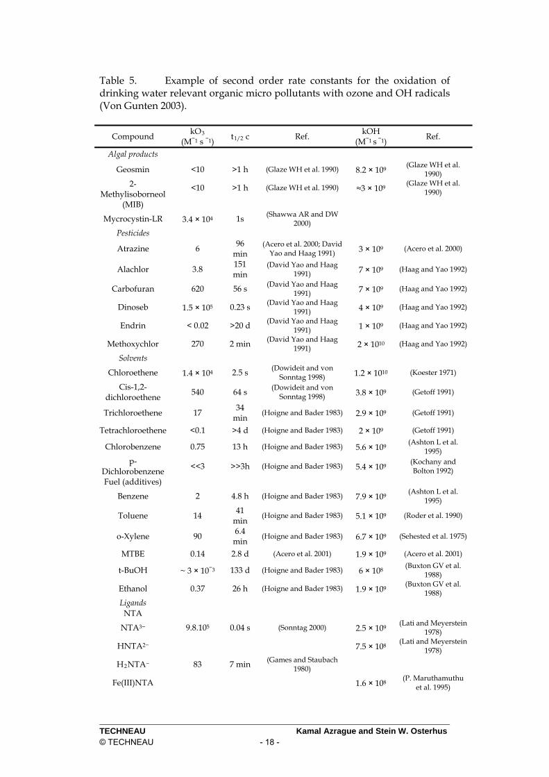
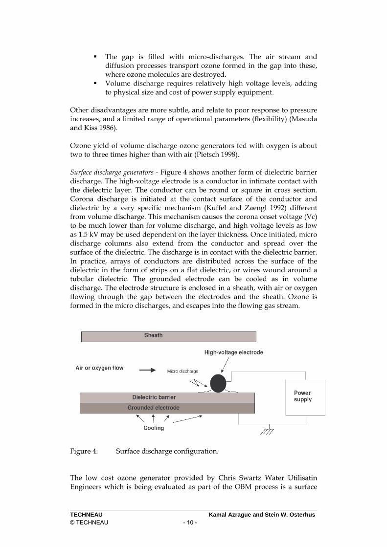
Table 5. Example of second order rate constants for the oxidation of drinking water relevant organic micro pollutants with ozone and OH radicals (Von Gunten 2003).

Compound kO3

(M−1 s −1) t1/2 c Ref.

kOH (M−1 s −1)

Ref.

Algal products

Geosmin <10 >1 h (Glaze WH et al. 1990) 8.2 × 109 (Glaze WH et al.

1990)

<10 >1 h (Glaze WH et al. 1990) ≈3 × 109 (Glaze WH et al.

1990) 2-

Methylisoborneol (MIB)

Mycrocystin-LR 3.4 × 104 1s (Shawwa AR and DW 2000)

Pesticides

Atrazine 6 96

min (Acero et al. 2000; David

Yao and Haag 1991) 3 × 109 (Acero et al. 2000)

Alachlor 3.8 151 min

(David Yao and Haag 1991) 7 × 109 (Haag and Yao 1992)

Carbofuran 620 56 s (David Yao and Haag 1991) 7 × 109 (Haag and Yao 1992)

Dinoseb 1.5 × 105 0.23 s (David Yao and Haag 1991) 4 × 109 (Haag and Yao 1992)

Endrin < 0.02 >20 d (David Yao and Haag 1991) 1 × 109 (Haag and Yao 1992)

Methoxychlor 270 2 min (David Yao and Haag 1991) 2 × 1010 (Haag and Yao 1992)

Solvents

Chloroethene 1.4 × 104 2.5 s (Dowideit and von Sonntag 1998) 1.2 × 1010 (Koester 1971)

Cis-1,2-dichloroethene

540 64 s (Dowideit and von Sonntag 1998) 3.8 × 109 (Getoff 1991)

Trichloroethene 17 34

min (Hoigne and Bader 1983) 2.9 × 109 (Getoff 1991)

Tetrachloroethene <0.1 >4 d (Hoigne and Bader 1983) 2 × 109 (Getoff 1991)

Chlorobenzene 0.75 13 h (Hoigne and Bader 1983) 5.6 × 109 (Ashton L et al.

1995) p-

Dichlorobenzene <<3 >>3h (Hoigne and Bader 1983) 5.4 × 109

(Kochany and Bolton 1992)

Fuel (additives)

Benzene 2 4.8 h (Hoigne and Bader 1983) 7.9 × 109 (Ashton L et al.

1995)

Toluene 14 41

min (Hoigne and Bader 1983) 5.1 × 109 (Roder et al. 1990)

o-Xylene 90 6.4

min (Hoigne and Bader 1983) 6.7 × 109 (Sehested et al. 1975)

MTBE 0.14 2.8 d (Acero et al. 2001) 1.9 × 109 (Acero et al. 2001)

t-BuOH ~ 3 × 10−3 133 d (Hoigne and Bader 1983) 6 × 108 (Buxton GV et al.

1988)

Ethanol 0.37 26 h (Hoigne and Bader 1983) 1.9 × 109 (Buxton GV et al.

1988) Ligands NTA

NTA3− 9.8.105 0.04 s (Sonntag 2000) 2.5 × 109 (Lati and Meyerstein

1978)

HNTA2− 7.5 × 108 (Lati and Meyerstein

1978)

H2NTA− 83 7 min (Games and Staubach 1980)

Fe(III)NTA 1.6 × 108 (P. Maruthamuthu

et al. 1995)


EDTA

HEDTA3− 1.6 × 105 0.2 s (Sonntag 2000) 2 × 109 (Lati and Meyerstein

1978)

EDTA4− 3.2 × 106 0.01 s (Sonntag 2000) 4 × 108 (Lati and Meyerstein

1978)

CaEDTA2− ≈ 105 0.35 s (Sonntag 2000) 3.5 × 109 (Lati and Meyerstein

1978)

Fe(III)EDTA 3.3 × 102 105 s (Sonntag 2000) 5 × 108 (Sharma and Sahul

1982) DTPA

CaDTPA3− 6200 6 s (Stemmler et al. 2001) Zn(HDTPA2−/H2

DTPA) ≈ 100 6 min (Stemmler et al. 2001) 2.3 × 109

(Stemmler et al. 2001)

ZnDTPA3− 3500 10 s (Stemmler et al. 2001)

Fe(III)(DTPA2−/ p10 X60 min

(Stemmler et al. 2001) 1.5 × 109 (Stemmler et al.

2001)

HDTPA) Fe(III)(OH)DTPA

3− 2.4 × 105 70 s (Stemmler et al. 2001)

Disinfection by-products

Chloroform ≤0.1 ≥100

h (Hoigne and Bader 1983) 5 × 107 (Haag and Yao 1992)

Bromoform ≤0.2 ≥50 h (Hoigne and Bader 1983) 1.3 × 108 (Haag and Yao 1992)

Iodoform < 2 >5 h (Bichsel 2000) 7 × 109 (Bichsel 2000)

Trichloroacetate <3 × 10_5 36 yr (Hoigne and Bader 1983) 6 × 107 (P. Maruthamuthu

et al. 1995) Pharmaceuticals

Diclofenac ~1 × 106 33 ms (Huber et al. 2003) 7.5 × 109 (Huber et al. 2003)

Carbamazepine ~3 × 105 0.1 s (Huber et al. 2003) 8.8 × 109 (Huber et al. 2003)

Sulfamethoxazole ~2.5 × 106 14 ms (Huber et al. 2003) 5.5 × 109 (Huber et al. 2003)

17α-Ethinylestradiol

~7 × 109 5 ms (Huber et al. 2003) 9.8 × 109 (Huber et al. 2003)

2.1.3.3 Hygenic barrier and disinfection Ozone is a strong and very efficient disinfectant, especially towards bacteria and viruses. It is also very efficient towards Giardia, but less efficient towards Cryptosporidium. The inactivation of micro organisms by ozone can be described by Chick’s law:

Log (N/No) = -k C T Where N is the number of organisms that remain viable, No is the initial number of viable organisms, k is the inactivation constant, C is the concentration of disinfectant (mg/L), and T is the exposure time (min). The relative impact of C and T is set to unity. The Chick’s law is the basis for design of the disinfection. In order to obtain a certain log inactivation of a certain type of target organism by ozone, a certain C T-value (the concentration of ozone times the contact time) is required. Tables 6, 7 and 8 show the required C T-values at different temperatures in order to obtain different log inactivation credit for the inactivation of Giardia, viruses and Cryptosporidium, respectively. There are no separate table for bacteria since they in general are more sensitive to ozone than i.e. viruses, and consequently inactivation of viruses ensures at least equal degree of inactivation of bacteria. The required C T-value found in tables 6, 7 and 8 (at the desired degree log


inactivation and temperature) would then be the design requirement for the disinfection by ozone giving the needed ozone concentration and contact time. Table 6. CT requirements to achieve inactivation of Giardia by ozone (USEPA 1991, Giudance manual for the compliance with the filtration and disinfection requirements for public water systems using surface water sources).

Temperature (ºC) Log inactivation ≤ 1 5 10 15 20 25

0,5 0,48 0,32 0,23 0,16 0,12 0,08 1,0 0,97 0,63 0,48 0,32 0,24 0,16 1,5 1,5 0,95 0,72 0,48 0,36 0,24 2,0 1,9 1,3 0,95 0,63 0,48 0,32 2,5 2,4 1,6 1,2 0,79 0,60 0,40 3,0 2,9 1,9 1,4 0,95 0,72 0,48 Table 7. CT requirements to achieve inactivation of viruses by ozone (USEPA 1991, Giudance manual for the compliance with the filtration and disinfection requirements for public water systems using surface water sources).

Temperature (ºC) Log inactivation ≤ 1 5 10 15 20 25

2,0 0,9 0,6 0,5 0,3 0,25 0,15 3,0 1,4 0,9 0,8 0,5 0,4 0,25 4,0 1,9 1,2 1,0 0,6 0,5 0,3 Table 8. CT requirements to achieve inactivation of Cryptosporidium by ozone using the T10 –method. (USEPA, LT2ESWTR).

Temperature (ºC) Log inactivation ≤

0,5 1 2 3 5 7 10 15 20 25

0,5 12 12 10 9,5 7,9 6,5 4,9 3,1 2,0 1,2 1,0 24 23 21 19 16 13 9,9 6,2 3,9 2,5 1,5 36 35 31 29 24 20 15 9,3 5,9 3,7 2,0 48 46 42 38 32 26 20 12 7,8 4,9 2,5 60 58 52 48 40 33 25 16 9,8 6,2 3,0 72 69 63 57 47 39 30 19 12 7,4


However, the design is not straight forward. The main question is which ozone concentration, C, and contact time, T, should be applied in the design. In general, the ozone consumed by other processes has to be accounted for since it is not available for disinfection. Similarly, short circuiting, dead volumes, etc also has to be taking into the consideration since it reduces the effective contact time. A common way to take the latter into account is using T10 (the time it takes for 90 percent of the water to pass the contactor) instead of the theoretical hydraulic detention time (HDT). Several methods to calculate the actual CT (in order to compare with the required C T-value for the design) may be used. USEPA discusses three main methods for calculating inactivation credit: the T10-method, the CSTR-method, and the Extended CSTR-method. The T10-method applies Ceffluent T10, but Caverage T10 may also be considered. The Extended CSTR-method may be used for Cryptosporidium inactivation and is applicable for compartmentalized ozone contactors such as over-under or serpentine baffled basins. The CSTR-method is a variation of the Extended CSTR-method and the T10-method and may be suitable for non-compartmentalized ozone contactors such as pipelines and long channels. USEPA are also considering other calculation methods. For more details about the design using the different methods we refer to the USEPA, Surface Water Treatment Rule (SWTR) Guidance Manual and USEPA, LT2ESWTR Toolbox Guidance Manual. Other countries may use more simplified calculation for the disinfection design. In Norway, a simplified version of the USEPA methods is suggested(Halvard Ødegaard et al. 2006).

2.1.4 Factors affecting the ozone system design Ozone is unstable in water. The decay of ozone in natural waters is characterized by a fast initial decrease of ozone, followed by a second phase in which ozone decreases with first-order kinetics. Depending on the water quality, the half-life of ozone is in the range of seconds to hours. This has to be taken into account when designing the ozone system. The major secondary oxidant formed from ozone decomposition in water is the OH radical (see figure 9).

Figure 9. Oxidation reaction pathways during ozonation of water.



The stability of ozone largely depends on the water matrix, especially its pH (high pH promotes ozone decomposition via OH radical), the type and content of natural organic matter (NOM) and its alkalinity (Hoigné 1998).

2.1.5 Alternative and additional oxidation methods The most common chemical oxidants used in water treatment are chlorine, ozone, chlorine dioxide, and permanganate. Free chlorine has traditionally been the oxidant (and disinfectant) of choice, but concerns about the formation of potentially harmful halogenated disinfection by-products (DBPs) produced by reactions between free chlorine and natural organic material (NOM), exacerbated in some cases by the presence of bromide, have caused many water systems to adopt alternative chemical oxidants (and disinfectants) to lower halogenated DBP formation. These other oxidants may also react with NOM and bromide to various degrees, depending upon the properties of the oxidant, to form oxidation by-products, some of which also have adverse public health effects or result in downstream operational problems in the treatment plant or distribution system. Recently, different studies have investigated the application of the advanced oxidation processes (AOP) to drinking water treatment to oxidize pollutants. The AOPs are defined as processes which involve reactions where takes place the accelerated production of the hydroxyl free radical (HO) which is the second strongest known oxidant (2.8 V) after fluorine. It is able to oxidize and mineralize almost every organic molecule, yielding CO2 and inorganic ions. The hydroxyl radical is nonselective with respect to its reactivity, in contrast to molecular ozone, which is highly selective in that its rate constants with various solutes range over more than 12 orders of magnitude. Atrazine, trichloroethylene, and tetrachloroethylene, all relatively inert toward molecular ozone, are oxidized at appreciable rates by the hydroxyl radical, and therefore by AOPs. Among the AOPs, the O3/high pH, O3/UV, O3/H2O2, UV/H2O2 and UV/TiO2 are the most promising system which can be applied within the OBM instead of the first ozonation step or in addition as for instance the UV/TiO2 can be applied as a final step to achieve a very low TOC level and to remove the trace of micropollutant which are difficultly removed by a single ozonation step.

2.2 Biodegradation When oxidizing organic matter, the biodegradable fraction or the AOC in the water typically increases. This fraction should be removed by a biodegradation step. In this report only biofiltration will be considered. Other types of biodegradtion reactors will be considered at a later stage.

2.2.1 Biofilter design Different authors (Wang et al. 1995) (Zhang and Huck 1996) have shown that the contact time with the biofilm is more important than the mass of biofilm above a minimum level of biomass. Generally, the longer the contact time the greater the removal of AOC. However, the increase in removal is not a linear-relationship; the removal rate decreases at extended contact times (Zhang and Huck 1996). Biofilter studies on the removal of ozonation by-products (aldehydes and keto-acids) demonstrated that their removal could be described well by a first order model in a plug flow reactor including a term for a minimum substrate concentration:

Sout = (Sin-Smin) . e-k + Smin Where Sin and Sout is the inlet and outlet concentration (µg/L), respectively, of substrate from the biofilter, Smin is the minimum substrate concentration that can maintain steady state biofilm (µg/L), k is the first order rate constant (min-1), and is the Empty Bed Contact Time, EBCT (min). Table 9 show example first order rate constants for the degradation of ozonation by-products in biofilters, and example of degradation of glyoxal at different starting concentrations and EBCT is shown in Figure 10. Table 9. Example of first order rate constants for degradation of ozonation by-products in biofilters. OBP k (min-1) Smin (µgl-1) OBP k (min-1) Smin (µgl-1)

Formaldehyde Glyoxal Methylglyoxal Acetone

0.39 0,21 0.22 0.19

1.0 – 3.0 <1 – 4.6 <1 – 2.2 <1 – 1.5

Glyozalic acid Pyruvic acid Ketomalonic acid

0.19 0.31 0.10

4.8 – 30 2.7 – 27 7.0 - 45

Figure 10. Example of degradation of an ozonation by-product (glyoxal) in a biofilter at different concentration and EBCT.


Bacteria which utilise readily available carbon is located in top layer (Moll SM et al. 1998) while bacteria able to degrade more recalcitrant carbon are living deeper in the filter. Griffini et al, (Griffini et al. 1999) observed that in steady-state, the removal of aldehydes and ketoacids most occurred at the top of the biofilter after 2.3 min EBCT. Little additional removal occurred in the rest of the biofilter. In case of BDOC, the samples taken along different biofilters showed also that majority of BDOC removal occurred in the top of the biofilter with some additional removal in the lower levels (Figure 11). The 10-15 min EBCT would have been enough in this case.

EBCT (min)

0 5 10 15 20 25

BD

OC

re

mov

al (

%)

0

20

40

60

80

100

GAC (Torbonite)GAC (Coconut shell)GAC (Wood)GAC (Bituminous)Biolite

Figure 11. BDOC removal in biofilters with samples taken along the filter column (Griffini et al, 1999). According to Uhl (Uhl 2000) such an empirical approach is very well suited to describe removal of DOC and AOC in biofilters. For process analysis the removal efficiency the removal efficiency ηz(x) for a parameter x at a given bed depth z is defined as:

fin

zinf

x

x- x z(x)

where the index inf indicated the value of the parameter at the influent e.g. BDOC or AOC. A maximal removal efficiency ηmax can be expressed and defined. If a first order reaction is assumed in the interstitial water of the bed, the removal efficiency as a function of bed depth can be calculated as:

EBCTbedkappze )(

max1


where kapp is apparent rate constant for a first order reaction, εbed is interstitial porosity and EBCT is empty bed contact time from influent to bed depth z. The parameters should be determined experimentally. Results of application of such model are shown in Figure 12.

Figure 12. Removal efficiency for AOC as function of bed depth and empirical modelling of a first order reactions (Uhl, 2000) In addition to the type and amount of substrate, several other factors are also important for the design of biofilters, such as temperature, nutrients, oxygen concentration, backwashing procedures, etc. Type of filter media also plays a role, but this is discussed in the chapter below. Nevertheless, typical EBCT range from 10 to 30 minutes.

2.2.2 Filter media in biofilters Any filter media which has sufficient surface area for microbes to attach to can be used for biological filtration. Slow sand, rapid sand, and GAC filters have all been successfully used for biologically active filtration. Biofilter media affects the amount of biomass accumulating in the biofilter (Table 10). Anthracite-sand removed also less OBPs at 12 min EBCT. Amount of biofilm in the biofilters does not directly compare with biofilter performance. Biofilm accumulation is highest at the top of the biofilter (in downflow filters) and amount of biofilm decreses along the filter depth (Wang et al., 1995) which correlates with high initial removal of BOM at the top layers of biofilter. Another advantage of GAC is that during start-up phase some of the organic matter (BDOC) is adsorbed while biological activity is building up (Carlson et al. 1994 ; Melin et al. 2002a; Servais et al. 1994). The length of adsorption phase can vary quite a lot depending on the type of GAC (Carlson et al., 1994).


Table 10. Biomass accumulation on biofilter media after 95 days (Wang et al., 1995).

Media Biomass nmol lipid-P g-1

media Mean Standard deviation

Anthracite prechlorinated 2.0 0.5 Anthracite backwashed with chlorinated

water 6.0 0.6

Anthracite 55.0 1.7 Sand 90.6 1.3

GAC1 (bituminous coal) 305 9 GAC2 (lignite coal) 465 9

GAC3 (wood) 382 11

2.3 Membrane filtration By introducing a biological step downstream the oxidation step (e.g. ozonation), growth may occur(Odegaard et al. 1999). Consequently a final filtration step is needed to reduce the possibility of pathogen growth into the network and the ingestion by waters users. Microfiltration (MF) and Ultrafiltration (UF) are low pressure or vacuum membrane filtration processes that are used for pathogen and suspended solids removal. MF/UF membrane processes have gained wide acceptance in the drinking water industry because of their ability to produce a high-quality and consistent product water. Thus, the candidate chosen for the final step is the membrane filtration. To imagine the advantages and limits for the design of membrane separation plants one has to consider the strong interrelationship between the feed in use, pretreatment, cleaning of the membrane separation plant, operating conditions and selection of the module (Fig. 13)(Gunther and Hapke 1996).


Figure 13 : Interrelationship for membrane plant deign In the present section different operational and design characteristics will be presented and from those characteristics a choice and operational method of membrane will be suggested for the OBM.

2.3.1 Membrane design characteristics Numerous manufacturers of MF/UF membrane systems exist, each with their own proprietary technologies. The differences between proprietary systems can be overwhelming and present significantly varying design considerations.

2.3.1.1 Types of UF/MF membrane systems Submerged Membrane Systems Submerged membrane systems are proprietary systems with Zenon and US Filter being the most prolific. Although the system components differ slightly between the manufacturers, the mode of operation remains similar regardless of the proprietary equipment used. Submerged membrane systems are those where the membrane fibers are immersed in an open tank and are exposed to the feed water. Groups of membrane fibers are bundled together in racks or modules. The membrane fibers are slightly longer than the distance between the upper and lower attachment points, allowing the membrane fiber to shake during operation to dislodge accumulated solids. Multiple modules can be submerged in the process tank, depending on the permeate flow required. During normal operation, raw water enters the process tank and completely submerges the


membrane modules. The raw water is drawn through the membrane fibers (outside-in) to the inside of the fiber (lumen) by a vacuum pump. Filtered water (permeate or filtrate) exits through the top of the module to the permeate manifold. Generally multiple modules are connected to one permeate pump through a common manifold. Concentrate is continuously withdrawn from the process tank so that the raw water flow is equal to the sum of both permeate and concentrate flow. Process tanks for submerged membrane systems are designed for a plug flow mode of operation, and recoveries will vary from 50% at the lead module to 99% at the end module. Suspended solids concentration also increases from the raw water inlet to the concentrate outlet. Since the solids concentration and module recovery increases from the lead module to the end module, flux decreases from the lead to the end module. However system recovery and flux is reported as an average of all modules.

Figure 14: Example of submerged membrane Submerged membrane systems can effectively replace clarifiers and multi-media type filters found in conventional water treatment plants and are capable of operating effectively and continuously in high solids environments. There is no need to create large flocculated particles for settling in clarifiers or for capture by granular media filters as the membranes are capable of removing pin flocs. Above 20000 m3 per day, capital and operating costs for submerged membrane systems are generally lower than encased membrane systems because of the need for less equipment and lower operating pressures. Additionally, submerged membrane systems can be particularly cost effective if an existing tank/basin can be utilized. Encased Membrane Systems Encased membrane systems are becoming increasingly non-proprietary in nature. As stated earlier, membrane elements from the various manufacturers are standardizing dimensions to allow for increased flexibility within a


particular system. This will allow for relatively simple changes to a system due to alterations in feed water quality, system performance standards, etc. The major manufacturers of UF are Pall, Koch, Norit (X-Flow), Aquasource, and Hydranautics. Encased membrane systems utilize the same hollow fibers as the submerged systems except that they are packed into a cylindrical casing, usually with a diameter of 200mm, and a length of 1m or 1,5m. These fiber packages, or elements, are then arranged end-to-end in a pipe, or vessel. Most commonly, in UF applications, the vessels are oriented vertically and each vessel houses one element. For large capacity systems – particularly in Europe – multiple modules can be installed in long vessels in a horizontal configuration similar to reverse osmosis systems. Some manufacturers provide their modules with end structures that are already configured to accept the required piping connections, thus eliminating the need for other housing. This can save a significant amount of capital cost. An encased system may utilize a cross-flow design, which can allow for a high flux with minimal solids build-up on the membrane surface, or it can operate in “dead-end” mode where all water processed through the filter comes out as filtrate.

Figure 15: Example of encased membrane

2.3.1.2 Membrane material properties Membranes can be manufactured in a wide variety of materials. These materials differ in their performance characteristics including mechanical strength, fouling resistance, hydrophobicity, hydrophilicity, and chemical tolerance. This section summarizes the differences in material properties. Membrane materials can be classified as either hydrophilic or hydrophobic. Hydrophilic means waterloving and such materials readily adsorb water. The


http://www.water-technology.net/projects/sulaibiya/index.html�

surface chemistry allows these materials to be wetted forming a water film or coating on their surface. Hydrophobic means water-hating and hydrophobic membrane materials have little or no tendency to adsorb water. Water tends to "bead" on hydrophobic surfaces into discrete droplets. The hydrophilic and hydrophobic properties of a membrane material are related to the surface tension of the material. The fundamental importance of surface tension comparison is that liquids having lower surface tension values will generally spread on materials of higher surface tension values. Table 11 below summarizes surface tension values of some polymeric membrane materials. The higher the surface tension value of the material, the more hydrophilic the material is. Table 11 : Calculated Surface Tension of Some Polymeric Materials

The degree of hydrophilicity or hydrophobicity influences the wettability and applied pressure requirements for water flow through the membrane. Hydrophilic membranes require less operating pressure than hydrophobic membranes. Hydrophilic membranes tend to exhibit greater fouling resistance than hydrophobic membranes. Particles that foul in aqueous media tend to be hydrophobic. Hydrophobic particles tend to cluster or group together to form colloidal particles because this lowers the interfacial free energy (surface tension) due to surface area exposure. General tendency will favor particle attachment to any material less hydrophilic than water because less exposure of hydrophobic particles can be achieved by attachment of the particles to the membrane surface. To prevent fouling, a membrane requires a surface chemistry which prefers binding to water over other materials. This implies that the material must be very hydrophilic. Membrane manufacturers offer membranes constructed of a wide variety of materials. These materials vary widely in their chemical and mechanical properties including mechanical strength, burst pressure, oxidant tolerance, VOC tolerance, pH operating range, and so forth. The end user must be aware of the strengths and limitation of each material type and ensure the selected material is compatible with raw water quality, pretreatment requirements, and other operating conditions.


2.3.1.3 Performance characteristics Flux Flux in a MF/UF membrane system is not a characteristic of a specific manufacturer so much as it is limited by the following parameters: • Raw water quality (temperature, solids content, NOM content, etc.). • Efficiency or existence of the pretreatment process. • Maximum transmembrane pressure as dictated by the physical properties of the membrane polymer and limitations of manufacturer’s equipment. • Acceptability of the resulting cleaning frequency All of these factors are interrelated and will therefore dictate the flux rate achievable on a case by case basis. Flux rates though can be as low as 8,5 LMH for challenging waters, and flux rates have been documented over 150 LMH for very clean feed waters. Average flux rates range from 40-70 LMH. Recovery Similar to flux, recovery rates in a MF/UF membrane system are not a characteristic of a specific manufacturer so much as recovery is limited by the following parameters: • Raw water quality (temperature, solids content, NOM content, etc.). • Efficiency or existence of the pretreatment process. • Maximum transmembrane pressure as dictated by the physical properties of the membrane polymer and limitations of manufacturer’s equipment. • Acceptability of the resulting cleaning frequency High recovery rates generally require high transmembrane pressures to operate higher cleaning frequencies because the membranes are forced to run in a higher solids environment. All of the above factors are interrelated and will therefore dictate the recovery rate achievable on a case by case basis. Recovery rates can be as low as 50% for challenging waters, while recovery rates have been documented at up to 99% for very clean feed waters. Average recovery rates range from 92% to 95%. Particle Rejection The main difference between membrane filtration and conventional filtration is that membranes reject particles based on size exclusion as opposed to media depth filtration. For all practical purposes, MF/UF membranes will produce a constant permeate water quality regardless of feedwater conditions because they act as an absolute barrier. This can be expected since most suspended solids present in raw water streams are larger than the pore size of most MF/UF elements. Permeate turbidity can be expected to be less than 0.1 NTU or lower and SDI less than 0.4. However, breaches in integrity such as a broken fiber or ruptured seal, or imperfections in the membrane due to the manufacturing process can allow particles to enter the permeate stream.


While it has been said that MF/UF membranes pose an absolute barrier to suspended solids, it is more appropriate to express solids removal in terms of log removal. Most membranes are capable of up to 6- log pathogen (protozoan cysts and bacteria) removal, though this will vary depending on the membrane manufacturer. Virus rejection varies significantly between manufacturers with some systems removing virtually no appreciable amount of viruses while others report greater than 6-log removal. Factors Affecting Fouling and Cleaning Frequency Fouling is the most serious disadvantage of pressure-driven membrane separation processes. Membrane fouling results in a decrease in flux and an increase in energy consumption and feed pressure. Fouling will occur in any MF/UF system, regardless of the membrane polymer, system manufacturer, and mode of operation. Fortunately, fouling can be effectively controlled through the proper use of pretreatment processes, chemical additions, and proper system design and operation. The following factors are the most common causes of membrane fouling and can be controlled by proper design and operation. Equipment Malfunctions. Malfunctioning equipment can increase cleaning frequencies. For example, malfunctioning level control equipment in a submerged membrane system can allow membranes to operate in partially full tanks, thus accelerating membrane fouling. Temperature. The effect of temperature on permeate flux is well documented in the membrane industry. Decreases in temperature decrease flux, increase TMP, and increase fouling rates. Cleaning frequencies can double with a 15-degree C change in water temperature. Flux. Increasing flux increases cleaning frequency. Recovery. Increasing recovery increases cleaning frequency due to higher solids concentrations in the feed water. For example, the solids concentration factor is 12.5 at 92% recovery and is 100 at 99% recovery. Cake Formation. Accumulation of particles near the surface of the membrane forms a cake layer which can be considered a second membrane. The cake layer can enhance the particle rejection characteristics of the membrane by depth filtration and adsorption. However, the cake layer increases the resistance to flux and leads to higher transmembrane pressures. This type of fouling is reversible and can be removed by cleaning and backpulsing. Adsorption. Organic matter present in the feedwater can lead to membrane fouling either be adsorbing into the cake formation or by adsorbing into the membrane itself. Some membrane polymers exhibit higher adsorptive rates than others, depending on the hydrophilicity of the polymer. Pretreatment can be optimized to remove as much organic matter from the feed to extend membrane life, and chemical cleaning can be optimized to remove adsorbed foulants.


Metals Precipitation. Though metals precipitation in MF/UF membranes is not as prevalent as in NF/RO processes, fouling due to metals precipitation has been documented. Calcium carbonate scale can form on the permeate side of membranes in scaling waters where carbon dioxide is driven off as part of the process. In operations using membrane filtration for iron and manganese removal, precipitation of these metals on the concentrate and permeate side can occur. Post-precipitation of iron and aluminium associated with metallic-based coagulants has been observed and can lead to fouling on the permeate side and increased particle counts in the permeate.

2.3.2 Design of the membrane filtration plant after the oxidation-biofiltration

2.3.2.1 Choice of the membrane The OBM can be assimilated to a membrane bioreactor (MBR) at list the two final steps. Thus, as it has been shown in the past for the MBR developments, the more suitable configuration of the UF or MF membrane module is a submerged membrane to avoid a high transmembrane pressure to maintain filtration. The reason also which can lead to this choice is that above 20000m3 per day, capital and operating costs for submerged membrane systems are generally lower than encased membrane systems. The selection of the membrane material depends considerably of the feed water coming from the bioreactor, the performance characteristics, the cost and the cleaning maintenance needed to remove the fouling which, in this case, is mainly biomass material (Le-Clech et al. 2006). As mentioned above, one has to choose a hydrophilic membrane because:

hydrophilic membranes require less operating pressure than hydrophobic membranes

And hydrophilic membranes tend to exhibit greater fouling resistance than hydrophobic membranes since the biomass is hydrophobic.

One alternative for the membrane module can be the ceramic membrane since the cost has decreased considerably.

2.3.2.2 Design of the plant The main objective of the design is to determine the total area of the membrane required for filtration. Towards this end, it is necessary to predict the permeate flux for the given influent characteristics and operating conditions which, in turn, depend on the membrane cleaning technique used. Once the optimal flux determined by taking into account the different parameters, an estimation of the membrane area needed can be done by using the following formulas (American Water Works Association (AWWA) 2005 ):

μR

TMP J

t


Where : J : instantaneous membrane flux (LMD) TMP: transmembrane pressure (psi) Rt : total membrane resistance (i.e. of the membrane resistance [Rm] and membrane fouling resistance [Rf] (psi/LMD-cP) µ: absolute viscosity of water (cP) Total filtrate production is:

Qt= Qp + Qbwp Where: Qt : total filtrate production (L/D) Qp: facility capacity (L/D) Qbwp: filtrate for backwashing (L/D) The membrane area required is:

.J

QA

t

Where: A : membrane area (m2) Qt : total filtrate production capacity (L/D) J: instantaneous membrane flux (LMD) η: online factor (dimensionless) The online factor is the percentage of time, expressed in decimal form, per day that the membrane system is producing filtrate. This parameter accounts for the amount of time lost because of backwashing, chemical cleaning, or other times when the membrane system is not producing filtrate. The online factor is:

η= 1-( ηbw + ηcip + ηother) Where: η: online factor ηbw: backwash online factor ηcip: CIP online factor ηother: other online factor (i.e. mini-clean) The number of membrane modules is:

modulemodules

A

A

Where: Modules: number of modules A: membrane area required Amodule: area per membrane module


The number of membrane units is:

unit

modules

Munits

Where: units: number of membrane units modules: modules Munit: modules per unit The recovery of the membrane facility is:

100f

p

Q

QR

Where: R: recovery (percent) Qf: total feed (L/D) Qp: facility capacity (L/D) The total amount of feed is:

Qf = Qp + Qbwp + Qbwf

Where:

Qf: total feed (L/D) Qp: facility capacity (L/D) Qbwp: filtrate used for backwashing (L/D) Qbwf: feed water for backwashing (L/D)


3 Preliminary cost assessment

The cost estimation is a very difficult task since all the three process within the OBM are strongly dependent on the water characteristics, in addition to the cost of the energy, land, etc which are different from place to place. However, based on different references, estimations for treatment plants with productions of 7 000, 20 000 and 100 000 m3/day have been made for a water containing 3 mg.L-1 of DOC using a specific ozone dose of 1 mg O3/mg DOC. The cost estimates are given in US dollar however an exchange rate of 1:1 between euro and US dollar could be used.

3.1 Ozonation For the ozone system, both capital and operating costs are key components for the overall cost estimate. Capital costs are the most difficult to estimate because there are many factors affecting the costs, such as level of instrumentation and automation, local construction costs, quantity of stainless steel piping (i.e., distance between equipment), and other factors. Charts that present capital cost estimates discussed here were obtained from Ozone in water treatment: Application and Engineering (Langlais et al. 1991b). These charts are 16 years old and were developed based on capital cost information for air-feed ozone systems. However, even though inflation has occurred over the years, the capital costs of a LOX-fed ozone system are lower and the charts are considered to still be applicable (Kerwin L. Rakness 2005).

3.1.1 Capital cost By using the method proposed Kerwin L. Rakness (Kerwin L. Rakness 2005) a capital cost can be calculated for different sizes of water treatment plants. The completed capital cost estimates for the different treatment plants are shown in the table 12. The contactor detention time chosen was 10 min, but longer or shorter detention times can be selected for the site-specific applications. Contactor cost increases as detention time increases, and vice-versa. For example, the costs will be 50% higher if the detention time is doubled to 20 min, or decrease by 25% if detention time is cut in half to 5 min. The total estimated ozone capital costs given below include costs for ozone equipment, ozone contactor, and ozone buildings. The estimates include equipment installation, but exclude other costs such as site work; design and construction management services; and owner’s administration, legal, and management expenses.



Table 12: Order of magnitude of the capital cost

Design Flow (m3/d) 7000 20000 100000

Ozone dose (mg/L) 3 3 3

Ozone production (kg/d) 21 60 300

Standby production (kg/d) 7 20 100

Installed generation capacity (kg/d) 28 80 400

Ozone equipment unit cost $/kg/d 23911 12786 4850

Projection equipment cost $ 669508 1022880 1940078

Anticipated contactor hydraulic detention time

Min 10 10 10

Projected contactor cost $ 500000 700000 1200000

Estimated unit building size m2/kg/d 0.51 0.44 0.34

Calculated building size m2 31.4 77.5 300

Estimated unit building cost $/m2 1625 1625 1625

Projected housing cost $ 51025 125937 487175

Total estimated ozone system cost

$ 1220533 1848817 3627253

3.1.2 O&M cost A completed calculated O&M costs form is shown in table 13 for the different size plants. O&M activities include daily equipment readings, spare parts replacement, preventive and emergency maintenance, and other activities. Table 13 : Order of magnitude of the operating cost

1. Operating information Average Annual Water Flow Rate m3/d Average Annual Dose mg/L

2. Average Annual Production kg/d 3. Estimated System Specific Energy kWh/kg 4. Estimated price of energy $/kWh 5. Estimated annual cost of energy $ 6. Estimated operating ozone concentration % 7. Estimated oxygen price $/kg O2 8. Estimated annual cost of oxygen $ 9. Estimated annual cost of energy and oxygen $ 10. Unit-Mass cost of ozone generation $/kg O3 11. Estimated cost factor of O&M % 12. Estimated annual cost for O&M $ 13. Total estimated ozone system annual operating cost $ 14. Unit-Volume cost of ozone $/m3 of treated water $/m3

7000

3 21 11

0.08 7419

10 0.09 6898

14909 1.86

20 2863

17181

0.0067

20000

3 60 11

0.08 21199

10 0.09

19710 40909

1.86 20

8181

49091

0.0067

100000

3 300 11

0.08 105996

10 0.09

98550 202356

1.86 20

40471

242827

0.0067

3.2 Biofiltration The O&M of the biofilter is considered negligible, and only the capital costs are considered. The empty bed contact time chosen for the biofilters is 20 min. The main factors affecting the price of the biofilter are the costs of the tanks, which depend largely on the materials used, and the costs of the housing/buildings requirements. The calculated biofiltration capital costs are shown in table 14. Table 14: Estimated biofiltration capital costs for three different size plants.

Production flow (m3/day) 7 000 20 000 100 000

Empty Bed Contact Time (min) 20 20 20

Stainless steal tanks ($) 287 000 820 000 4 100 000

Estimated unit building cost ($/m2)1625 1625 1625

Calculated building size (m2) 65 185 926

Housing/buildings ($) 52 650 300 950 1 504 750

3.3 Membrane filtration The American Water Works Association (AWWA) has developed a method to estimate the different capital and O&M costs for membrane systems (American Water Works Association 2005). Therefore we have used this approach to estimate the costs of the membrane filtration for the different treatment plant sizes chosen. All the calculations are given with accuracy of ±25%.

3.3.1 Capital cost The estimates are made for a water of high quality (low turbidity, low TOC) or where pre-treatment has been used to reduce the TOC of the feed water and increase the membrane flux, which is the case for the OBM process. This estimation has been made for a water temperature of 20˚C which has to be corrected if the temperature is different since it affects the water viscosity and consequently the flux. The calculated capital costs of the UF membrane filtration for the considered plant sizes are shown in table 15. Table 15: Estimated membrane filtration capital and O&M costs for three different sizes

Production flow (m3/day) 7 000 20 000 100 000 Capital cost ($) 748 000 1 602 000 4 770 000 Membrane facilities cost ($) 1 870 000 3 738 000 12 190 000 O&M ($) 72 562 188 340 843 150


3.3.2 O&M cost The O&M costs for the UF membrane filtration are given in table 15. The estimates have been made based on the following assumptions: • Energy

- Includes feed backwash pumps or intermittent air (e.g., air during backwashing) usage. - Electricity is 0.08 $/kWh. - No available or residual pressure requirements before or after the membrane system.

• Chemical washing - Daily use with sodium hypochlorite solution or applied with each backwash - Waste solution disposal via onsite neutralization or disposal to sewer at nominal cost, excluding neutralisation and any sewer connection volume charges or impact fees

• Chemical cleaning - Monthly frequency - Two separate cleanings using acid followed by sodium hydroxide or sodium hypochlorite with CIP reuse, if appropriate - Waste solution disposal via onsite neutralization or disposal to sewer, excluding neutralisation and any sewer connection volume charges or impact fees

• Membrane replacement - Assumes year-round operation at design capacity - ”Standard” membrane warranty (e.g., full replacement during first year and a pro-rata replacement in the range of 7 to 10 years)

• Exclusions/qualifiers - Equipment maintenance allowance not included (typically 0.004 to 0.008 $/m3) - Disposal or treatment cost for backwash water not included - No pre-treatment chemical costs - Cost of waste disposal excluded - Operates at design capacity year-round - No labour costs are included

3.4 Total cost Estimate of the OBM Table 16 presents the total estimated costs for OBM treatment plants with a capacity of 7 000, 20 000 or 100 000 m3/day. The capital costs were annualised considering an amortisation factor calculated as a function of the interest rate for capital investments (6%) and for a design life of the plant of 20 years. The annualised total capital cost was expressed as cost per unit volume of treated water produced in order to compare it with the operating costs and obtain the total treatment cost. The calculated total treatment costs for the OBM process are competitive with the costs for conventional water treatment (coagulation-sedimentation-sand filtration) which is assumed to be 0.25 $/m3 for a production of 20 000 m3/day (M. R. Wiesner et al. 1994; Pianta et al. 2000). According to these


estimations the main O&M and capital costs of the OBM process are due to the membrane filtration. Nevertheless, this step is needed to have an improved water quality. However, the costs per m3 are already lower than for conventional treatment plants, and since the prices on membranes are continuously decreasing, the OBM concept is very promising. Indeed, a new generation of ozone generator is able to produce ozone at lower energy consumption (Masuda and Kiss 1986; Masuda et al. 1986), and due to a competitive market, further cost reductions on membranes will be realized in coming decades. In addition to the cost reductions on membranes, membrane developments will permit higher fluxes, enhanced fouling mitigation/control and more efficient ways to operate membrane systems (S. Caothien et al. 2003), e.g. as it is for submerged membrane systems (Freeman et al. 2003). Table 16: Total costs estimation for the OBM with production flows of: 7 000, 20 000 and 100 000 m3/day

Production flow m3/day 7 000 20 000 100 000

Capital cost of equipment ($) 4 178 183 8 309 767 26 192 003

Number of years 20 20 20

Interest rate (%) 6 6 6 Amortization of capital

Annual payment ($) 359 205 714 396 2 251 764

Operational costs Annual O&M ($) 89 743 237 431 1 085 977

Total treatment cost Annual treatment cost ($) 448 948 951 827 3 337 741

Treatment cost ($/m3) produced

0.17 0.13 0.09


References Acero, J. L., Haderlein, S. B., Schmidt, T. C., Suter, M. J. F., and von Gunten,

U. (2001). "MTBE Oxidation by Conventional Ozonation and the Combination Ozone/Hydrogen Peroxide: Efficiency of the Processes and Bromate Formation." Environ. Sci. Technol., 35(21), 4252-4259.

Acero, J. L., Stemmler, K., and von Gunten, U. (2000). "Degradation Kinetics of Atrazine and Its Degradation Products with Ozone and OH Radicals: A Predictive Tool for Drinking Water Treatment." Environ. Sci. Technol., 34(4), 591-597.

American Water Works Association. (2005). "Microfiltration and Ultrafiltration membranes for drinking water.".

American Water Works Association (AWWA). (2005 ). "Microfiltration and Ultrafiltration membranes for drinking water.".

Ashton L, Buxton GV, and CR., S. (1995). "Temperature-dependence of the rate of reaction of OH with some aromatic compounds in aqueous solution — evidence of the formation of pi-complex intermediate." J Chem Soc Faraday Trans 91, 1631-3.

Baral, S., Lume-Pereira, C., Janata, E., and Henglein, A. (1986). "Chemistry of colloidal manganese oxides. 3. Formation in the reaction of hydroxyl radicals with manganese(2+) ions." J. Phys. Chem., 90(22), 6025-6028.

Bichsel, Y. (2000). "Behavior of iodine species in oxidative processes during drinking water treatment." PhD thesis, Swiss Federal Institute of Technology, Zürich, .

Bielski, B. H. J., and Allen, A. O. (1977). "Radiation chemistry of aqueous cyanide ion." J. Am. Chem. Soc., 99(18), 5931-5934.

Buxton GV, Greenstock CL, Helman WP, and WP., R. (1988). "Critical review of rate constants for reactions of hydrated electrons, hydrogen atoms and hydroxyl radicals in aqueous solution." J Phys Chem Ref Data 17, 513-886.

Carlson, M. A., Heffernan, K. M., Ziesemer, C. C., and Snyder, E. G. (1994 ). "Comparing two GACs for adsorption and biostabilization." Journal AWWA, 86(3 ), 91-102.

David Yao, C. C., and Haag, W. R. (1991). "Rate constants for direct reactions of ozone with several drinking water contaminants." Water Research, 25(7), 761-773.

DeMers, L. D., and Renner, R. C. (1992). "Alternative Disinfection Technologies for Small Drinking Water Systems." AWWARF and AWWA, Denver, CO.

Dimitriou, M. A. (1990). "Design Guidance Manual for Ozone Systems." International Ozone Association, Norwalk, CN.

Dowideit, P., and von Sonntag, C. (1998). "Reaction of Ozone with Ethene and Its Methyl- and Chlorine-Substituted Derivatives in Aqueous Solution." Environ. Sci. Technol., 32(8), 1112-1119.

Frank Jacobsen, J. H. K. S. (1998). "Oxidation of manganese(II) by ozone and reduction of manganese(III) by hydrogen peroxide in acidic solution." International Journal of Chemical Kinetics, 30(3), 207-214.

Freeman, S., Henderson, R., and Veerapaneni, V. (2003). "Procurement methods for low-pressure membrane filtration plants. Proceedings of


the Pacific Northwest SectionAWWA Conference, Boise, Idaho, May 2003. CD-ROM. AmericanWaterWorks Association, Denver, Colo."

Games, L. M., and Staubach, J. A. (1980). "Reaction of nitrilotriacetate with ozone in model and natural waters." Environ. Sci. Technol., 14(5), 571-576.

Getoff, N. (1991). "Radiation- and photoinduced degradation of pollutants in water. A comparative study." International Journal of Radiation Applications and Instrumentation. Part C. Radiation Physics and Chemistry, 37(5-6), 673-680.

Glaze WH, Schep R, Chauncey W, Ruth WH, Zarnoch JJ, M., Aieta E, Tate CH, and MJ., M. (1990). "Evaluating oxidants for the removal of model taste and odor compounds from a municipal water supply." J Am Water Works Assoc 87(5), 79-84.

Griffini, O., Bao, M. L., Barbieri, K., Burrini, D., Santianni, D., and Pantani, F. (1999). "Formation and removal of biodegradable ozonation by-products during ozonation-biofiltration treatment: Pilot-scale evaluation." Ozone Science & Engineering, 21, 79-98.

Gunther, R., and Hapke, J. (1996). "Design of membrane separation plants using a module data base." Desalination, 104(1-2), 119-128.

Halvard Ødegaard, Fiksdal, L., and W.Østerhus, S. (2006). "Optimal desinfeksjonspraksis for drikkevann." Hamar : Norsk vann og avløp.

Hickel, B., and Sehested, K. (1992). "Reaction of hydroxyl radicals with ammonia in liquid water at elevated temperatures." International Journal of Radiation Applications and Instrumentation. Part C. Radiation Physics and Chemistry, 39(4), 355-357.

Hoigné, J. (1998). Chemistry of aqueous ozone, and transformation of pollutants by ozonation and advanced oxidation processes., The handbook of environmental chemistry quality and treatment of drinking water. Berlin: Springer.

Hoigne, J., and Bader, H. (1983). "Rate constants of reactions of ozone with organic and inorganic compounds in water--I : Non-dissociating organic compounds." Water Research, 17(2), 173-183.

Hoigne, J., Bader, H., Haag, W. R., and Staehelin, J. (1985). "Rate constants of reactions of ozone with organic and inorganic compounds in water--III. Inorganic compounds and radicals." Water Research, 19(8), 993-1004.

Huber, M. M., Canonica, S., Park, G. Y., and von Gunten, U. (2003). "Oxidation of Pharmaceuticals during Ozonation and Advanced Oxidation Processes." Environ. Sci. Technol., 37(5), 1016-1024.

Haag, W. R., and Hoigne, J. (1983). "Ozonation of bromide-containing waters: kinetics of formation of hypobromous acid and bromate." Environ. Sci. Technol., 17(5), 261-267.

Haag, W. R., and Yao, C. C. D. (1992). "Rate constants for reaction of hydroxyl radicals with several drinking water contaminants." Environ. Sci. Technol., 26(5), 1005-1013.

Jayson GG, Parsons BJ, and AJ., S. (1972). "Oxidation of ferrous ions by hydroxyl radicals." J Chem Soc Faraday Trans, 18, 229-33.

Karmann W, Meissner G, A., H., Naturforsch, Z., and B, T. (1967;:). 22, 273-82.


Kerwin L. Rakness. (2005). "Ozone in Drinking Water Treatment: Process Design, Operation, and Optimization." Amer Water Works Assn.

Kim, M.-J., and Nriagu, J. (2000). "Oxidation of arsenite in groundwater using ozone and oxygen." The Science of The Total Environment, 247(1), 71-79.

Klaening, U. K., Bielski, B. H. J., and Sehested, K. (1989). "Arsenic(IV). A pulse-radiolysis study." Inorg. Chem., 28(14), 2717-2724.

Kochany, J., and Bolton, J. R. (1992). "Mechanism of photodegradation of aqueous organic pollutants. 2. Measurement of the primary rate constants for reaction of hydroxyl radicals with benzene and some halobenzenes using an EPR spin-trapping method following the photolysis of hydrogen peroxide." Environ. Sci. Technol., 26(2), 262-265.

Koester, R. (1971). Z Naturforsch Teil B, 26, 1108-16. Kuffel, E., and Zaengl, W. S. (1992). High Voltage Engineering Fundamentals.

Pergamon Press. Langlais, B., D., R., and Brink, D. (1991a). "Ozone in Water Treatment:

Application and Engineering." Lewis Publishers, Inc., Chelsea, MI. Langlais, B., Reckhow, D., and Brink, D. (1991b). Ozone in Water Treatment:

Application and Engineering, Lewis Publishers, Inc., Chelsea, MI. Lati, J., and Meyerstein, D. (1978). "Oxidation of first-row bivalent transition-

metal complexes containing ethylenediaminetetra-acetate and nitrilotriacetate ligands by free radicals: a pulse-radiolysis study." J. Chem. Soc., Dalton Trans., 1105 - 1118.

Le-Clech, P., Chen, V., and Fane, T. A. G. (2006). "Fouling in membrane bioreactors used in wastewater treatment." Journal of Membrane Science, 284(1-2), 17-53.

Loegager, T., Holcman, J., Sehested, K., and Pedersen, T. (1992). "Oxidation of ferrous ions by ozone in acidic solutions." Inorg. Chem., 31(17), 3523-3529.

Loegager, T., and Sehested, K. (1993). "Formation and decay of peroxynitrous acid: a pulse radiolysis study." J. Phys. Chem., 97(25), 6664-6669.

M. R. Wiesner, J. H. Hackney, S. Sethi, J. G. J., and J. M. Laîné. (1994). "Cost estimates for membrane filtration and conventional treatment, ." J. AWWA 86 .(12), 33-41.

Malley, J. P., Eighmy, T. T., Collins, M. R., Royce, J. A., and D.F.Morgan. (1993). "The True Performance and Microbiology of Ozone - Enhanced Biological Filtration." J. AWWA., 85(12), 47-57.

Masuda, S., and Kiss, E. (1986). Proc. 1986 Annual Conf. of Inst. Electrostatics Japan, 209 - 212.

Masuda, S., Sato, M., and Seki, T. (1986). IEEE Trans. On Industry Appl. Vol No IA, 22(5), 886 - 891.

Melin, E., Eikebrokk, B., Brugger, M., and H., Ø. (2002a). "Treatment of Humic Surface Water at Cold Temperatures by Ozonation and Biofiltration." Water Science and Technology: Water Supply, , 2(5-6), 451-457.

Melin, E., Eikebrokk, B., Brugger, M., and Ødegaard, H. (2002b). "Treatment of humic surface water at cold temperatures by ozonation and biofiltration." Water science & technology : Water supply, 2(5-6), 451–457.


Melin, E. S., and Odegaard, H. (1999). "Biofiltration of ozonated humic water in expanded clay aggregate filters." Water Science and Technology, 40(9), 165-172.

Moll SM, Summers RS, and A, B. (1998). "Microbial characterization of biological filters used for drinking water treatment" Applied and Environmental Microbiology, , 64(7), 2755-2759.

Odegaard, H., Eikebrokk, B., and Storhaug, R. (1999). "Processes for the removal of humic substances from water-- An overview based on norwegian experiences." Water Science and Technology, 40(9), 37-46.

P. Maruthamuthu, Padmaja, S., and Huie, R. E. (1995). "Rate constants for some reactions of free radicals with haloacetates in aqueous solution." Int J Chem Kinet 27, 605-612.

Pianta, R., Boller, M., Urfer, D., Chappaz, A., and Gmunder, A. (2000). "Costs of conventional vs. membrane treatment for karstic spring water." Desalination, 131(1-3), 245-255.

Pietsch, G. J. (1998). Gas discharges in ozone generators. Regional Conference on Ozone Generation and Application to Water and Waste Water Treatment. Moscow, Russia 26-28 May 13 - 28.

Renner, R. C., M.C. Robson, G.W. Miller, and Hill., A. G. (1988). "Ozone in Water Treatment -The Designer’s Role." Ozone Sci. Engrg., 10(1), 55-87.

Rice, R. G. (1996). "Ozone Reference Guide. Electric Power Research Institute, St. Louis, MO."

Roder, M., Wojnarovits, L., and Foldiak, G. (1990). "Pulse radiolysis of aqueous solutions of aromatic hydrocarbons in the presence of oxygen." International Journal of Radiation Applications and Instrumentation. Part C. Radiation Physics and Chemistry, 36(2), 175-176.

S. Caothien, C. Liu, and O´Connell, P. (2003). "Reducing fouling and the cost of membrane systems." Proceedings of the 2003 AWWA Membrane Technology Conference, 2-5 March 2003, Atlanta, Ga CD-ROM, American Water Works Association, Denver Colo.

Sehested, K., Corfitzen, H., Christensen, H. C., and Hart, E. J. (1975). "Rates of reaction of oxygen(1-) ions, hydroxyl radicals, and atomic hydrogen with methylated benzenes in aqueous solution. Optical spectra of radicals." J. Phys. Chem., 79(4), 310-315.

Servais, P., Billen, G., and Bouillot, P. (1994). "Biological colonization of granular activated carbon filters in drinking-water treatment.".Journal of Environmental Engineering, 120(4 ), 888-899.

Sharma, B. K., and Sahul, K. (1982). "60Co y-radiolysis of iron(III)nitrolotriacetate in aqueous solutions." Radiation Physics and Chemistry (1977), 20(5-6), 341-346.

Shawwa AR, and DW, S. (2000). "Kinetics of microcystin-LR oxidation by ozone." Ozone Sci Eng 23, 161-70.

Sonntag, F. M. a. C. v. (2000). "The reactions of ozone with tertiary amines including the complexing agents nitrilotriacetic acid (NTA) and ethylenediaminetetraacetic acid (EDTA) in aqueous solution." J. Chem. Soc., Perkin Trans. , 2, 2029 - 2033.

Stemmler, K., Glod, G., and von Gunten, U. (2001). "Oxidation of metal-diethylenetriamine-pentaacetate (DTPA) - complexes during drinking water ozonation." Water Research, 35(8), 1877-1886.



Uhl, W. (2000). "Biofiltration processes for organic matter removal." Biotechnology, Environmental Processes III, Wiley-VCK, Weinheim, New Your, 11, 457-478.

Von Gunten, U. (2003). "Ozonation of drinking water: Part I. Oxidation kinetics and product formation." Water Research, 37(7), 1443-1467.

Von Gunten U, Bruchet A, and E., C. (1996). "Bromate formation in advanced oxidation processes." J. Amer. Water Works Assoc., 88(6), 53-65.

Wang, J. Z., Summers, R. S., and Miltner, R. J. (1995). "Biofiltration performance: part 1, relationship to biomass." Journal AWWA, 87((12), 55-63.

Zhang, S., and Huck, P. M. (1996). "Removal of AOC in biological water treatment processes: A kinetic modeling approach." Water Research, 30(5), 1195-1207.

Fundamental process design principles for the OBM ... · PDF fileFundamental process design...

Documents

Transcript of Fundamental process design principles for the OBM ... · PDF fileFundamental process design...