Fundamental Limitations ofSemi-Supervised Learning

by

Tyler (Tian) Lu

A thesispresented to the University of Waterloo

in fulfillment of thethesis requirement for the degree of

Master of Mathematicsin

Computer Science

Waterloo, Ontario, Canada, 2009

c© Tyler (Tian) Lu 2009

Declaration

I hereby declare that I am the sole author of this thesis. This is a true copy of thethesis, including any required final revisions, as accepted by my examiners.

I understand that my thesis may be made electronically available to the public.

ii

Abstract

The emergence of a new paradigm in machine learning known as semi-supervisedlearning (SSL) has seen benefits to many applications where labeled data is ex-pensive to obtain. However, unlike supervised learning (SL), which enjoys a richand deep theoretical foundation, semi-supervised learning, which uses additionalunlabeled data for training, still remains a theoretical mystery lacking a sound fun-damental understanding. The purpose of this research thesis is to take a first steptowards bridging this theory-practice gap.

We focus on investigating the inherent limitations of the benefits semi-supervisedlearning can provide over supervised learning. We develop a framework underwhich one can analyze the potential benefits, as measured by the sample com-plexity of semi-supervised learning. Our framework is utopian in the sense that asemi-supervised algorithm trains on a labeled sample and an unlabeled distribution,as opposed to an unlabeled sample in the usual semi-supervised model. Thus, anylower bound on the sample complexity of semi-supervised learning in this modelimplies lower bounds in the usual model.

Roughly, our conclusion is that unless the learner is absolutely certain there issome non-trivial relationship between labels and the unlabeled distribution (“SSLtype assumption”), semi-supervised learning cannot provide significant advantagesover supervised learning. Technically speaking, we show that the sample complexityof SSL is no more than a constant factor better than SL for any unlabeled distri-bution, under a no-prior-knowledge setting (i.e. without SSL type assumptions).

We prove that for the class of thresholds in the realizable setting the samplecomplexity of SL is at most twice that of SSL. Also, we prove that in the agnosticsetting for the classes of thresholds and union of intervals the sample complexityof SL is at most a constant factor larger than that of SSL. We conjecture this tobe a general phenomenon applying to any hypothesis class.

We also discuss issues regarding SSL type assumptions, and in particular thepopular cluster assumption. We give examples that show even in the most accom-modating circumstances, learning under the cluster assumption can be hazardousand lead to prediction performance much worse than simply ignoring unlabeleddata and doing supervised learning.

This thesis concludes with a look into future research directions that builds onour investigation.

iii

Acknowledgements

I would like to thank my advisor, Shai Ben-David, for his support, encourage-ment, and guidance throughout my Master’s studies. I have benefitted a great dealfrom my advisor’s high standards of scholarship and intellectually engaging style.

It has been a pleasure to work with my collaborators and colleagues Alex Lopez-Ortiz, Kate Larson, David Pal, Martin Pal, Teresa Luu, Rita Ackerman, MiroslavaSotakova, Sharon Wulff, Pooyan Khajehpour, and Alejandro Salinger. In addition,I like thank my office mates Ke Deng, Jakub Gawryjolek, Ting Liu, Sharon Wulff,Derek Wong, and Teresa Luu for creating a livelier atmosphere at work.

I like to thank some faculty members including Pascal Poupart, Joseph Cheriyan,Peter van Beek, Anna Lubiw, Yuying Li, Jochen Konemann, and Ali Ghodsi forteaching great courses or having interesting discussions on various topics.

I like to thank Pascal Poupart and Ming Li for reading my thesis and providingvaluable and insightful feedback.

Lastly I would like to thank my parents and my extended family for their un-conditional support and hope in me.

iv

Contents

List of Figures vii

1 Introduction 1

1.1 Outline of Thesis . . . . . . . . . . . . . . . . . . . . . . . . . . . . 4

2 Background in Statistical Learning Theory 6

2.1 Some Notation . . . . . . . . . . . . . . . . . . . . . . . . . . . . . 6

2.2 Motivating the Probably Approximately Correct Model . . . . . . . 8

2.3 The Agnostic PAC Model . . . . . . . . . . . . . . . . . . . . . . . 10

2.4 The Realizable PAC Model . . . . . . . . . . . . . . . . . . . . . . . 12

2.5 Learnability and Distribution-Free Uniform Convergence . . . . . . 13

2.5.1 Agnostic Setting . . . . . . . . . . . . . . . . . . . . . . . . 14

2.5.2 Realizable Setting . . . . . . . . . . . . . . . . . . . . . . . . 16

3 Modelling Semi-Supervised Learning 18

3.1 Utopian Model of Semi-Supervised Learning . . . . . . . . . . . . . 19

3.2 Related Work . . . . . . . . . . . . . . . . . . . . . . . . . . . . . . 21

3.2.1 Previous Theoretical Approaches . . . . . . . . . . . . . . . 24

3.3 Issues with the Cluster Assumption . . . . . . . . . . . . . . . . . . 25

4 Inherent Limitations of Semi-Supervised Learning 30

4.1 Fundamental Conjecture on No-Prior-Knowledge SSL . . . . . . . . 31

4.2 Reduction to the Uniform Distribution on [0, 1] . . . . . . . . . . . 34

4.2.1 The Rough Idea . . . . . . . . . . . . . . . . . . . . . . . . . 35

4.2.2 Formal Proof . . . . . . . . . . . . . . . . . . . . . . . . . . 36

4.3 Learning Thresholds in the Realizable Setting . . . . . . . . . . . . 40

4.4 Thresholds and Union of Intervals in the Agnostic Setting . . . . . 48

4.5 No Optimal Semi-Supervised Algorithm . . . . . . . . . . . . . . . 54

v

5 Conclusion 56

5.1 Proving Conjectures 4.1 and 4.2 . . . . . . . . . . . . . . . . . . . . 57

5.2 Verifying SSL Assumptions . . . . . . . . . . . . . . . . . . . . . . . 57

5.3 SSL Sample Complexity Incorporating Assumptions . . . . . . . . . 58

APPENDICES 60

A Examples of VC Dimension 61

A.1 Thresholds . . . . . . . . . . . . . . . . . . . . . . . . . . . . . . . . 61

A.2 Union of Intervals . . . . . . . . . . . . . . . . . . . . . . . . . . . . 62

A.3 Linear Halfspaces . . . . . . . . . . . . . . . . . . . . . . . . . . . . 62

References 63

vi

List of Figures

1.1 Guarantees can be proved for supervised learning . . . . . . . . . . 2

1.2 Can guarantees be proved for semi-supervised learning? . . . . . . . 3

2.1 Example of the overfitting phenomenon . . . . . . . . . . . . . . . . 9

3.1 Example of problems with the cluster assumption on mixture of twoGaussian with same shape. . . . . . . . . . . . . . . . . . . . . . . . 27

3.2 Example of problems with the cluster assumption on mixture of twovery different Gaussians . . . . . . . . . . . . . . . . . . . . . . . . 28

3.3 Example of problems with the cluster assumption on mixture of twohomogeneous labeled distributions . . . . . . . . . . . . . . . . . . . 28

4.1 Reducing to the Uniform Distribution on [0, 1] . . . . . . . . . . . . 35

4.2 Illustrating the algorithm of Kaariainen (2005) . . . . . . . . . . . . 41

4.3 A sample complexity lower bound for distinguishing two similarBernoulli distributions. . . . . . . . . . . . . . . . . . . . . . . . . . 50

4.4 Example of a b-shatterable triple (R2,H, D) . . . . . . . . . . . . . 52

4.5 Union of at most d intervals 2d-shatters the uniform distribution over[0, 1] . . . . . . . . . . . . . . . . . . . . . . . . . . . . . . . . . . . 54

A.1 Class of thresholds . . . . . . . . . . . . . . . . . . . . . . . . . . . 61

vii

“The beginning of knowledge is the discov-ery of something we do not understand.”

— Frank Herbert (1920 - 1986)

viii

Chapter 1

Introduction

Machine learning is a field that is broadly concerned with designing computer al-gorithms that learn from experience or automatically discover useful patterns fromdatasets. Much theory and applied work have been focused in the area of super-vised learning, where the goal is to approximate a ground truth function f : X → Ywhere X is some domain, and Y is some label class. For example, X can be theset of all digital pictures, Y a set of some persons, and f tells us who appearsin the photograph. Of course, our purpose is for the machine to automatically“learn” f , that is, output a function approximating f , based on an input collectionof examples, of say, pictures and their correct labels, known as the training data,

(x1, y1), (x2, y2), . . . , (xm, ym), each xi ∈ X , yi ∈ Y .

In supervised learning, the theoretical frameworks defining learnability, the cor-responding mathematical results of what can be learned, and the tradeoffs betweenlearning an accurate predictor and the available training data are reasonably wellunderstood. This has been a major success in the theoretical analysis of machinelearning—a field known as computational learning theory, and statistical learningtheory when computational complexity issues are ignored. Many practically im-portant learning tasks can be cast in a supervised learning framework. Examplesinclude predicting a patient’s risk of heart disease given her medical records, mak-ing decisions about giving loans, face recognition in photographs, and many otherimportant applications. See Figure 1.1 for an example of a theoretically soundsupervised learning paradigm.

Outside of supervised learning, however, our current theoretical understandingof two important areas known as unsupervised learning and semi-supervised learning(SSL) leaves a lot to be desired. Unsupervised learning is concerned with discoveringmeaningful structure in a raw dataset. This may include grouping similar datapoints together, known as clustering, or finding a low dimensional embedding ofhigh dimensional input data that can help in future data prediction problems,known as dimensionality reduction.

1

Figure 1.1: Supervised learning: a maximum margin linear classifier separatingcircles and crosses. Guarantees on future predictions can be given.

Semi-supervised learning, as the name suggests, is the task of producing a pre-diction rule given example data predictions (labeled data) and extra data withoutany prediction labels (unlabeled data). See Figure 1.2 for an illustration. In manypractical scenarios, labeled data is expensive and hard to obtain as it usually re-quires human annotators to label the data, but unlabeled data are abundant andeasily obtainable. Consequently, researchers are interested in using unlabeled datato help learn a better classifier. Due to numerous applications in areas such as nat-ural language processing, bioinformatics, or computer vision, this use of auxiliaryunlabeled data has been gaining attention in both the applied and theoretical ma-chine learning communities. While semi-supervised learning heuristics abound (seefor example, Zhu, 2008), the theoretical analysis of semi-supervised learning is dis-tressingly scarce and does not provide a reasonable explanation of the advantagesof unlabeled data.

While it may appear that learning with the addition of unlabeled data ismagical—after all, what can one learn from data that does not provide any clueon a function that is to be approximated?—In fact most practitioners performingSSL make some type of assumptions on how the labels behave with respect to thestructure of the unlabeled data. In practice, this may provide great advantage. Forexample, a popular assumption asserts that a good predictor should go througha low density region of the data domain. However, the focus of this thesis is ona more fundamental question: what can be gained when no assumptions of abovetype are made? While this question may seem far from practical interest, it is afirst step towards the theoretical modelling of practical SSL and understanding itslimitations.

In this thesis, we focus on formalizing a mathematical model of semi-supervisedlearning and analyze its potential benefits and inherent limitations when compared

2

?

Figure 1.2: Semi-supervised learning: the extra boxes represent unlabeled data, butwhere to place the separator? What can be proved about the future performance?

with supervised learning. Our model is based on the Probably ApproximatelyCorrect (or PAC) learning framework proposed by Valiant (1984). The main con-clusion of our thesis is:

Unless the learner is absolutely sure of an assumption that holds onthe relationship between labels and the unlabeled data structure (if noassumptions are made then we refer to it as the no-prior-knowledgesetting) then one cannot hope to obtain a significant advantage in thesample complexity1 of semi-supervised learning over that of supervisedlearning.

See Chapter 4 for a precise statement. When SSL assumptions are made but do nothold, it can degrade the performance and can be worse than supervised learning (seeSection 3.3. The semi-supervised learning model used in our analysis is one in whichthe learner is provided with a labeled training sample and complete knowledge ofthe distribution generating unlabeled data. Of course, this differs from the real-world model where a sample of unlabeled data is given. However, our analysis showsthat even in such an optimistic scenario that we assume, one still cannot obtainbetter than constant factor improvement in the labeled sample complexity. Thisis done by proving lower bounds on the labeled sample complexity of SSL, whichalso applies to supervised learning, and comparing that with the upper bounds onthe labeled sample complexity of supervised learning, which also applies to SSL. Inthis thesis we are mainly concerned with lower bounds in our SSL model. At the

1Sample complexity refers to the amount of labeled training data needed to learn an accurateclassifier. An alternate measure is the error rate of the learned classifier, which happens to dependon the sample complexity.

3

same time, upper bounds in our SSL model apply to the real-world SSL model asthe unlabeled sample size grows.

We also show that common applications of SSL that assume some relationshipbetween labels and the unlabeled data distribution (such as the widely held clusterassumption that prefers decision boundaries through low density region) may leadto poor prediction accuracy, even when the labeled data distribution does satisfy theassumption to a large degree (e.g. the data comes from a mixture of two Gaussiandistributions, one for each class label).

Our thesis is not the first work on the merits of using unlabeled data withoutmaking assumptions regarding the relationship between labels and the unlabeleddata distribution. The transductive learning model of Vapnik (2006) and its per-formance bounds do not make SSL type assumptions. However, the transductivemodel is concerned with prediction of a fixed, unlabeled test data set rather thangeneralizing a predictor for all points in a domain. As well, Kaariainen (2005) pro-poses some SSL algorithms that do not depend on SSL type assumptions. Mean-while, the work of Balcan and Blum (2005, 2006) offers a PAC style frameworkfor formalizing SSL type assumptions. We discuss more about how our work com-pares with respect to these approaches and other related works in Section 3.2. Thefundamental difference with our work is that we are interested in understandingthe inherent limitations of the benefits that semi-supervised learning provides oversupervised learning, whereas some of the related work is on providing “luckiness”conditions under which SSL can be successful.

This thesis does not completely provide answers to the question of the merits ofsemi-supervised learning. But it does show that for some relatively natural classesof prediction functions over the real line, semi-supervised learning does not helpsignificantly unless additional assumptions are made. We also believe the resultsgeneralize to other classes of functions, as asserted in our conjectures in Section 4.1.Much of the results contained in this thesis has already appeared in preliminaryform Ben-David et al. (2008).

1.1 Outline of Thesis

Chapter 2. We first present some background material on the statistical learningtheory of supervised learning that will be essential to understanding our proposedformulation of semi-supervised learning in the later chapters. This chapter willstart off with a brief expository tour of the main motivations and issues that mustbe addressed by a formal framework of learning, while presenting definitions alongthe way that will ultimately lead to constructing a formal framework of learningknown as the Probably Approximately Correct (PAC) learning framework (Valiant,1984). We also discuss the subtleties of PAC learning.

In the last part of the chapter, we review a seminal result of Vapnik and Chervo-nenkis (1971) on empirical process theory and its relationship in fully characterizing

4

the informational requirements of PAC learning. Important theorems will be statedthat provide upper and lower bounds on the sample complexity, in other words, howmuch training data is needed to learn well.

Chapter 3. In this chapter we will motivate and present a utopian model of semi-supervised learning as well as definitions corresponding to measuring its samplecomplexity. We will then briefly describe related work on SSL from the perspec-tive of our work. We will also discuss in detail and critique previous theoreticalparadigms for SSL including the shortcomings of these approaches. Then we turnour attention to an important issue for practitioners performing SSL, that of the po-tential hazards of learning under the popular cluster assumption. We give examplesof scenarios that appear to be amenable for learning with the cluster assumption,but in actuality damages learning.

Chapter 4. We propose a fundamental conjecture under the no-prior-knowledgesetting2 that roughly asserts SSL cannot provide significant advantages over super-vised learning. Then, for the remaining part of the chapter we turn our attentionto proving the conjecture for some basic hypothesis classes over the real line.

For “natural” hypothesis classes over the real line, we present a reduction lemmathat reduces semi-supervised learning under “smooth” distributions to supervisedlearning under the fixed uniform distribution on the unit interval, while preservingits sample complexity. Using this lemma, we are able to prove the conjecture for theclass of thresholds in the realizable setting, and thresholds and union of intervalsthe agnostic setting. We also examine a different formulation of comparing SSLwith supervised learning with negative conclusions for SSL.

Chapter 5. We finally conclude by taking a step back and providing generalcommentary on the big picture of semi-supervised learning and what insights ourresults give. We describe three open questions for future research into the theory ofsemi-supervised learning, and offer some general directions researchers can take.

2when no assumptions are made on the relationship between labels and the unlabeled datastructure.

5

Chapter 2

Background in StatisticalLearning Theory

Before presenting a new framework for the theoretical analysis of semi-supervisedlearning, we will first review some background material on supervised learning the-ory, also known as statistical learning theory. Our framework will be an extensionof the usual Probably Approximately Correct (PAC) model of Valiant (1984) for su-pervised learning. We will also cover its “agnostic” version (Haussler, 1992; Kearnset al., 1992, 1994). Since this thesis is mostly concerned with the informationalor statistical aspects of learning—either supervised or semi-supervised—we avoidissues of computational complexity of learning, the study of such issues along withstatistical aspects is sometimes known as computational learning theory.

For a more comprehensive and pedagogical treatment of the material in thischapter, we refer the reader to the following expository works: Anthony and Bartlett(1999); Kearns and Vazirani (1994); Devroye et al. (1997); Vapnik (1998).

In the rest of this chapter, we will first lay down the notation in Section 2.1to be used throughout the thesis. Then in Section 2.2 we give an expository tourof the motivation behind the various aspects and definitions of the PAC model.In Section 2.3 and 2.4 we formally define notions of a learning algorithm and thesample size requirements of learning algorithms. Finally, in Section 2.5 we describethe incredible connection between characterizing learning and the seminal workof Vapnik and Chervonenkis (1971) on the foundations of statistics.

2.1 Some Notation

While we will also develop notation for new definitions found throughout the re-mainder of this thesis, we will now present some notation that can be digested forthe reader without a background in statistical learning theory. For backgroundin probability theory at the measure theoretic level, see for example (Billingsley,1995).

6

• Let X denote the input domain of a classification problem, Y = 0, 1, andS0 a σ-algebra over X . We define a measure space (X × Y ,S) where theσ-algebra S consists of sets of the form A × B where A ∈ S and B ⊆ Y .Typically, we will assume the input data to a learning algorithm are drawnindependently from some probability measure over this space (see Section 2.2for more details).

• For a probability distribution P , we denote by Pm the product distributionP × · · · × P︸ ︷︷ ︸

m times

.

• For a random variable X,

– we denote X ∼ P if X is distributed according to a probability distri-bution P ,

– we denote PrX∼P (A) the probability that X ∈ A of a measurable set A,

– and we denote the expectation of X with respect to P by EX∼P (X).

• For a probability distribution P over X×Y we denote P (Y |X) the conditionaldistribution of Y given X.

• For a positive integer n, denote [n] = 1, 2, . . . , n.• We use := to indicate a definition of an equality.

• For a subset T of a domain set, we use 1T to denote its characteristic function(i.e. equals to 1 if x ∈ T and 0 otherwise).

• We use R and N to denote the real numbers and non-negative integers, re-spectively.

• We use O(·) for the big-O notation, Ω(·) for big-omega notation and Θ(·) forbig-theta notation.

• We use for function composition.

• For an indicator function I over some domain X , we define set(I) := x ∈X : I(x) = 1.• For two sets A and B we denote their symmetric difference by A∆B =

(A\B) ∪ (B\A).

The next section we will discuss some issues in formalizing a model of compu-tational learning, and hence motivate the concepts of the Probably ApproximatelyCorrect model.

7

2.2 Motivating the Probably Approximately Cor-

rect Model

Let us begin with some basic definitions.

Definition 2.1. The labeled training data is a collection

(x1, y1), (x2, y2), . . . , (xm, ym)

where for each i ∈ [n], (xi, yi) ∈ X ×Y . Each element of the collection is known asan example.

In this thesis, we will let Y = 0, 1, which is known as the classification setting.When Y is a continuous set, then it is known as the regression setting.

For convenience we will sometimes refer to labeled training data as labeled data,labeled sample or simply training data. As an example of the above definitions, ifwe are interested in automatically classifying email as spam or not spam, we canmodel this by letting X be the set of all possible emails (e.g. represent it as a bag ofwords vector), 0 as not spam and 1 as spam. We want to design a spam detectingalgorithm that takes as input labeled training data and outputs a predictor forfuture emails.

Definition 2.2. A hypothesis (or predictor, or classifier) is a function h : X → Ysuch that h−1(1) ∈ S0, for a σ-algebra S0 over X . That is, the set representationof h, denoted by set(h) = h−1(1), is measurable. A hypothesis class (or space) 1 H

is a set of hypotheses.

Intuitively the input training data must be “representative” of future emailsotherwise you cannot learn useful rule for future prediction. For example, onecannot expect a student to do well in an exam on linear algebra if a classroomteacher always gives homework questions on calculus. The PAC model overcomesthis issue by assuming that the training data and future test data are sampled i.i.d.(independently, identically distributed) according to some fixed, but unknown (tothe learning algorithm) distribution P .

Definition 2.3. A data generating probability distribution, or a labeled distribution,P is a probability measure defined over (X × Y ,S).

Thus, the input training data is a random variable distributed according to Pm

where m is the training data size. Our aim is to design a learning algorithm thatgiven the training data, outputs a hypothesis h with low future error on examplesfrom P .

1Technically we should require that H be permissible, a notion introduced by Shai Ben-Davidin (Blumer et al., 1989) which is a “weak measure-theoretic condition satisfied by almost allreal-world hypothesis classes” that is required for learning.

8

Definition 2.4. Let P be a distribution over X × Y , and S be a labeled trainingsample. The true error of a hypothesis h with respect to P is

ErP (h) := E(x,y)∼P

(h(x) 6= y) = P(x, y) : h(x) 6= y.

The empirical error of a hypothesis h with respect to S is the fraction of misclassifiedexamples,

ErS(h) :=|(x, y) ∈ S : h(x) 6= y|

|S| .

Note that the curly braces above represent a collection rather than a set. TheBayesian optimal hypothesis with respect to P is

OPTP (x) =

0 if P (y = 0|x) ≥ 1/2,

1 otherwise.

It is easy to see that the Bayesian optimal classifier is the function with thesmallest possible error. Of course, we usually do not have access to P otherwisethe learning problem simply becomes outputting the Bayesian optimal.

Now we are almost ready to define what it is for an algorithm to learn. Oneattempt is to say that an algorithm learns if when we are given more and morelabeled data, we can output hypotheses that get closer and closer in true error tothe Bayesian optimal. However, there is one huge problem: a phenomenon knownas overfitting.

Figure 2.1: Which predictor is better—the “complicated” shape which makes nomistakes on separating the training data or the simple linear separator that makessmall mistakes? Occam’s razor: “one should not increase, beyond what is necessary,the number of entities required to explain anything.”

Here is an informal example that captures the essence of overfitting: a class-room teacher gives some questions and answers, there is a student who learns bymemorizing all the question and answers, should the student expect to do well on

9

an exam? If the exam questions are the same as those given earlier, then the stu-dent will do perfectly, but if the exam has entirely different questions then quitepossibly not. The major issue here is that it is difficult for the student to assessher own exam performance if she has not seen the exam, even though she can doperfectly given previously seen questions. In our setting, the exam plays the roleof future data to classify while questions and answers are training data. See 2.1 fora pictorial example. Below is a more formal example.

Example 2.1 (Overfitting). Let X = [0, 1] and P be such that its marginal over Xis the uniform distribution and for all x ∈ [0, 1], P (y = 1|x) = 1. For any m > 0,suppose a training sample is drawn S = (x1, y1), . . . , (xm, ym) ∼ Pm. Considerthe hypotheses

1x1, . . . , xm =

1 if ∃i ∈ [m], x = xi

0 otherwise, h(x) = 1.

Clearly ErP (h) = ErS(h) = 0. On the other hand ErS(χS) = 0, but ErP (χS) =P(x, y) /∈ S = 1. However, since the input to any algorithm is only S, it cannotdecide how to label the remaining points outside of S because the sample error maybe far from the P -error. How does the PAC model fix this?

2.3 The Agnostic PAC Model

The solution to overfitting in the PAC framework is to restrict oneself to a hypoth-esis class H that is in some way not “complex” (i.e. cannot be too rich a class thatcan overfit), and require that a learning algorithm be one in which the larger theinput training data, the closer the error of the algorithm’s output hypothesis to thebest hypothesis in H.

Definition 2.5. Let X be a domain, Y = 0, 1, and H a hypothesis class. Asupervised learning algorithm with respect to H is an algorithm

A :∞⋃i=0

(X × Y)i → YX ,

(YX is the set of all possible functions from X → Y) such that for every (ε, δ) ∈(0, 1]2, there exists a non-negative integer m such that for all probability distribu-tions P over X ×Y , with probability at least 1− δ over a random sample S ∼ Pm,

ErP (A(S))− infh∈H

ErP (h) ≤ ε .

The parameters ε and δ are referred to as the accuracy and confidence parameters,respectively. The above probability and condition can be succinctly written as

PrS∼Pm

(ErP (A(S))− inf

h∈HErP (h) ≤ ε

)≥ 1− δ . (2.1)

10

Occasionally we will be using the term supervised algorithm to refer to any algorithmthat takes training data and outputs a hypothesis (i.e. it does not need to “learn”).

Several things to note in the definition. First, the learning requirement isdistribution-free : there is a sample size for A that only depends on ε, δ,H suchthat for any data generating distribution P drawing a sample of size m(A, ε, δ,H)from P suffices to learn within ε accuracy and δ confidence. This may seem like avery strong condition, but one of the crowning achievements of learning theory isthat this condition can be satisfied given H is a “nice” class (see Section 2.5).

Second, the ε accuracy condition is relative to the “best” predictor in H (thebest may not exist, but for any ξ > 0 there exist predictors with true errors thatare ξ-close). We only require the learner do well with respect to the best in H andnot necessarily the Bayesian optimal. Of course, learning would not be interestingif one does not fix a H whose best hypothesis has small error. In the extreme case,if no hypothesis in H has less than 50% error, then learning is trivially achieved byoutputting a classifier that flips a fair coin to guess a label. Thus,

the learner must use her prior knowledge to choose an appropriate H

that contains a hypothesis with small error.

However, there’s another issue, as we have seen in Example 2.1 and as we will seein Section 2.5, if a H is chosen with “too many” functions in the hopes that it willinclude a hypothesis with low error, one runs into problems with overfitting. Thus,the learner faces a tradeoff in specifying a H that contains a hypothesis with lowerror and not having a class of “rich” functions.

Third, the algorithm can output any hypothesis, not just ones inside H. Theonly requirement is that the true error of the output hypothesis is close to the trueerror of the “best” hypothesis in H. For example, the algorithm may even restrictits output predictors to lie inside another hypothesis class H′ that does not overlapwith H.

While in the original PAC formulation the learning algorithm must run in poly-nomial time with respect to the training sample size, in this thesis we will ignore anycomputational complexity issues. Instead we focus on informational complexity.

Definition 2.6. We define the supervised learning (SL) sample complexity withrespect to supervised algorithm A, ε, δ > 0, hypothesis class H, and distribution Pover X × Y as

mSL(A, ε, δ,H, P ) := min

m

∣∣∣∣ PrS∼Pm

(ErP (A(S))− inf

h∈HErP (h) ≤ ε

)≥ 1− δ

and we define the supervised learning sample complexity as

mSL(ε, δ,H) := minA

supPmSL(A, ε, δ,H, P ).

11

That is, the sample complexity tells us that there exists a learning algorithmsuch that if the training data is of size at least mSL(ε, δ,H) then we can obtainaccuracy ε and confidence δ. If the input data size is any less than mSL(ε, δ,H)then there is no algorithm that can obtain the desired accuracy and confidence.The sample complexity for supervised learning and semi-supervised learning (to bedefined later) is the main focus of this thesis. In essence, we are interested in seeingif it is smaller for SSL compared with SL.

2.4 The Realizable PAC Model

What we have described in the previous section is the known as the agnostic ex-tension of the original PAC model. It is so-called because one does not assumeanything about the Bayesian optimal classifier—it can have positive error or it canhave zero error and may not lie inside H. In this section we describe the originalPAC model, one that assumes the labels of data generating distribution come fromsome hypothesis in H.

Definition 2.7. Fix H over X ,Y . A hypothesis h is a target hypothesis if theunderlying data generating distribution P over X ×Y has the property that P (y =h(x)|x) = 1. More succinctly, ErP (h) = 0. For such a P , we rewrite it as Ph. Therealizable setting occurs if a target hypothesis exists in H.

Indeed, the realizable assumption is quite strong: the learner must know inadvance that the Bayesian optimal has zero error and must lie in the chosen hy-pothesis class. On the other hand, one can obtain better bounds on the samplecomplexity (see Section 2.5). The modified definition of a learning algorithm is thesame as in Definition 2.5 except the set of distributions is restricted to those thatrespect the realizable property.

Definition 2.8. A supervised learning algorithm for realizable setting with respectto H is an algorithm

A :∞⋃i=0

(X × Y)i → YX ,

such that for every (ε, δ) ∈ (0, 1]2, there exists a non-negative integer m such thatfor all probability distributions Pg over X × Y , where g ∈ H,

PrS∼Pm

g

(ErPg(A(S))− inf

h∈HErPg(h) ≤ ε

)≥ 1− δ .

We will often use the term supervised learning algorithm to refer to both therealizable and agnostic settings, and it will be clear which definition is being usedby the context. The sample complexity can be defined analogously to Definition 2.6(again, we will use the term SL sample complexity to refer to both agnostic andrealizable settings).

12

Definition 2.9. We define the supervised learning (SL) sample complexity for re-alizable setting with respect to supervised algorithm A, ε, δ > 0, hypothesis classH, and distribution Pg over X × Y where g ∈ H as

mSL(A, ε, δ,H, Pg) := min

m

∣∣∣∣ PrS∼Pm

g

(ErPg(A(S))− inf

h∈HErPg(h) ≤ ε

)≥ 1− δ

and we define the supervised learning sample complexity for realizable setting as

mSL(ε, δ,H) := minA

supPg :g∈H

mSL(A, ε, δ,H, Pg).

Going back to address the issue in Example 2.1 on overfitting, we will now turnour attention to “complexity” or “richness” property of H that will affect both theissue of whether a learning algorithm exists at all and how the sample complexitydepends on it.

2.5 Learnability and Distribution-Free Uniform

Convergence

It turns out that there is a beautiful connection between PAC learning and the sem-inal work of Vapnik and Chervonenkis (1971) on empirical process theory. Roughly,their result says that given H is not too complex (to be defined shortly) then it ispossible to estimate the true error of all hypotheses via the sample error given asufficiently large sample that does not depend on the data generating distribution.Before we formally state this main theorem, we need to develop the notion of thecomplexity of H that will characterize PAC learning.

Definition 2.10. Let X be a domain, Y = 0, 1, and H a hypothesis class overX ,Y . For h ∈ H and a set A = a1, . . . , am ⊆ X let h(A) := (h(a1), . . . , h(am)) ∈Ym. Define the growth function as follows,

Π(m,H) := maxA⊆X :|A|=m

|h(A) : h ∈ H|.

For a set A such that |h(A) : h ∈ H| = 2|A| we say that H shatters A. TheVapnik-Chervonenkis dimension of H is the size of the largest shatterable set,

VC(H) := sup m : Π(m,H) = 2m

To see some examples of the VC dimension of some basic classes such as unionof intervals and linear halfspaces, refer to Appendix A.

The VC(H) fully characterizes uniform convergence of estimates of sample errorto the true error, with explicit upper and lower bounds on the convergence ratethat match to within a constant factor. The supremum in the definition of theVC-dimension covers the case when VC(H) = ∞, in which case, as we will see,imply no learning algorithm exists that can compete with the best hypothesis inH.

13

2.5.1 Agnostic Setting

Let us first state an upper bound on the uniform convergence. This result was firstproved by Vapnik and Chervonenkis (1971) and subsequently improved on withresults from Talagrand (1994) and Haussler (1995).

Theorem 2.1 (Distribution-Free Uniform Convergence). Fix a hypothesis classH over X ,Y = 0, 1. There exists a positive constant C, such that for everyε, δ ∈ (0, 1]2, if

m ≥ C

ε2

(VC(H) + ln

(1

δ

))then for every probability distribution P over X × Y,

PrS∼Pm

(∀h ∈ H,∣∣ErS(h)− ErP (h)

∣∣ ≤ ε) ≥ 1− δ . (2.2)

One may also express ε in terms of given values of m and δ or express δ asa function of ε and m. The crucial features of uniform convergence is that it isdistribution-free as discussed earlier, and the condition inside (2.2) holds for allhypotheses in H.

This uniform convergence result leads to a very natural, intuitive, and naivealgorithm: given a training sample S, pick any hypothesis h that has the smallestempirical error in H.

Definition 2.11 (ERM Paradigm). Given a training sample S, the empirical riskminimization paradigm is any algorithm that outputs a hypothesis with minimumsample error,

ErS(ERM(S)) = minh∈H

ErS(h) .

This is only a statistical principle and does not consider the computationalcomplexity of finding the empirical minimizer. We note that ERM actually refersto a class of possible algorithms that outputs the empirical error minimizer as ournext example shows.

Example 2.2 (Different ERM Algorithms). Suppose we are learning initial seg-ments (or thresholds) over X = R, that is, hypotheses

H = 1(∞, a] : a ∈ Rand our data generating distribution P is such that the marginal P over R is theuniform distribution over the unit interval, and the conditional

P (y = 1|x) =

1 if x < 1/2

0 otherwise,

so that 1(−∞, 1/2] has zero error. Now when a training sample

S = (x1, y1), . . . , (xm, ym)

14

is drawn i.i.d. from P , we can have several different ERM approaches. For simplicityreorder the indices of the sample so that x1 ≤ x2 ≤ · · · ≤ xm, and let ` = maxxi :yi = 1 and r = minxi : yi = 0.

LeftERM(S) = 1(−∞, `] (2.3)

RightERM(S) = 1(−∞, r)

ERMRandom(S)(x) =

1 if x ≤ `

0 if x ≥ r

1 with probability 1/2

RandomERM(S) ∼ Bernoulli(LeftERM(S),RightERM(S), 1/2). (2.4)

The deterministic algorithm ERMRandom outputs a stochastic classifier that out-puts a random guess in the interval [x`, xr], this is different than the randomizedalgorithm RandomERM that flips a fair coin and outputs the classifier LeftERM(S)or RightERM(S). Note that we need not output a hypothesis in H, just one that hassmallest empirical error with respect to those in H (of course we need to be carefulwith overfitting). For the rest of this thesis, we will assume that ERM chooses ahypothesis in H with smallest empirical error.

Now, this is the stage where we show the connection between uniform conver-gence and sample complexity. Namely, that uniform convergence justifies the ERMprinciple, which in turn imply an upper bound on the SL sample complexity.

Theorem 2.2 (Agnostic Supervised Learning Upper Bound). Let C be the constantin Theorem 2.1, and

m0 :=4C

ε2

(VC(H) + ln

(1

δ

)). (2.5)

If m ≥ m0 then for any distribution P over X × Y,

PrS∼Pm

(ErP (ERM(S))− inf

h∈HErP (h) ≤ ε

)≥ 1− δ .

In other words the SL sample complexity mSL(ε, δ,H) ≤ m0.

Proof. Let2 h∗P := argminh∈H ErP (h). By Theorem 2.1, assuming m ≥ m0, thenfor all P , with probability 1− δ over sample S, the following holds,

ErP (ERM(S)) ≤ ErS(ERM(S)) +ε

2by (2.2)

≤ ErS(h∗P ) +ε

2by definition of ERM

≤(

ErP (h∗P ) +ε

2

)+ε

2by (2.2)

= ErP (h∗P ) + ε ,

which is exactly the requirement from (2.1) for learning.

2While the optimal hypothesis in H with respect to P may not exist, we can take a hypothesisthat gets close enough to the infimum for the proof to follow through.

15

It turns out that ERM is optimal with respect to the SL sample complexity, upto constant factors. The following is a corresponding lower bound for the samplecomplexity (i.e. no algorithm has better than constant sample complexity). Thislower bound essential results from Vapnik and Chervonenkis (1974).

Theorem 2.3 (Agnostic Supervised Learning Lower Bound). For (ε, δ) ∈ (0, 1/64)2,

mSL(ε, δ,H) ≥ VC(H)

320ε2

if H contains at least two hypotheses then for ε ∈ (0, 1) and δ ∈ (0, 1/4), we alsohave

mSL(ε, δ,H) ≥ 2

⌊1− ε2ε2

ln1

8δ(1− 2δ)

⌋The proofs of Theorem 2.1 and Theorem 2.3 can be found in the expository

book of Anthony and Bartlett (1999, Chap. 4 and 5, respectively). Now we willturn our focus to the sample complexity of the realizable setting where one makesthe strong assumption that a zero error hypothesis lies in the chosen hypothesisspace.

2.5.2 Realizable Setting

For the realizable setting (see the definition in Section 2.4) there are better samplecomplexity bounds. Basically, the ε2 in the denominator of the sample complex-ity upper bound (see Equation (2.5)) reduces to ε. The corresponding algorithmwhich matches the sample complexity upper bounds is, unsurprisingly, ERM. Thefollowing upper bound was originally proved by Blumer et al. (1989).

Theorem 2.4 (Realizable Supervised Learning Upper Bound). The supervisedlearning sample complexity, mSL(ε, δ,H), for the realizable setting satisfies

mSL(ε, δ,H) ≤ 4

ε

(VC(H) ln

(12

ε

)+ ln

(2

δ

)).

This bound is achieved by ERM which outputs any hypothesis that is consistent withthe training sample.

The following lower bound, which matches the upper bound up to a factor ofln(1/ε), first appeared in Ehrenfeucht et al. (1989).

Theorem 2.5 (Realizable Supervised Learning Lower Bound). The supervisedlearning sample complexity, mSL(ε, δ,H), for the realizable setting satisfies

mSL(ε, δ) ≥ VC(H)− 1

32ε

and if H contains at least two hypotheses then for ε ∈ (0, 3/4) and δ ∈ (0, 1/100),

mSL(ε, δ) >1

2εln

(1

δ

).

16

The proofs of these bounds can also be found in (Anthony and Bartlett, 1999,Chap. 4 and 5).

Now we are ready to move onto the next chapter of this thesis, where we willpresent a new model for semi-supervised learning that is based on the PAC modeldiscussed in this chapter.

17

Chapter 3

Modelling Semi-SupervisedLearning

In this chapter we will present a new, formal mathematical model for semi-supervisedlearning. This model is “utopian,” where we assume that the distribution of theunlabeled data is given to the semi-supervised learner. The intuition here is thatunlabeled data is abundant and cheap and that the learner can essentially “re-construct” the distribution over the unlabeled data. From this point of view ofsemi-supervised learning, any positive result in the usual model of SSL, where asample of unlabeled data is given rather than an entire distribution, is a positiveresult in our utopian model. And of course, any inherent limitations of this utopianSSL model implies inherent limitations in the usual model. Our model is based onthe Probably Approximately Correct (PAC) model of Valiant (1984) and also itsagnostic version (Haussler, 1992; Kearns et al., 1992, 1994). See Chapter 2 forbackground on PAC learning.

The purpose of this new model is to analyze SSL in a clean way without dealingwith unlabeled data sampling issues, and to also compare the potential gains ofthis utopian model of SSL with that of supervised learning. This last part willbe investigated further in Chapter 4. This chapter will be devoted to presentingthe model, discussions about the model, and how it fits with related work on thepractice and theory of SSL.

In Section 3.1 we present the new model of semi-supervised learning, its motiva-tions and consequences for the ordinary model of semi-supervised learning. We dis-cuss related work in Section 3.2 on the theory of semi-supervised learning and howthey are unsatisfactory, as well as putting into perspective various approaches—both practically and theoretically inspired—in the use of unlabeled data. In Sec-tion 3.3 we investigate (naturally occurring) scenarios that can hurt semi-supervisedlearning under the practically popular “cluster assumption,” and show the inher-ent dangers with using inaccurate prior knowledge about the relationship betweenlabels and the unlabeled data structure.

18

3.1 Utopian Model of Semi-Supervised Learning

In the usual setup for semi-supervised learning a learner is given training data thatconsists of labeled data

(x1, y1), (x2, y2), . . . , (xm, ym) ∈ X × Y

and in addition, unlabeled data

xm+1, xm+2, . . . , xm+u ∈ X ,

and the goal, or rather hope, is to output a hypothesis h : X → Y that is betterthan what we can get from the labeled data alone. In applications such as nat-ural language processing or computer vision the unlabeled data is typically muchmore abundant than labeled data. Whereas labeled data may need to be obtainedthrough the use of specialized human annotators (e.g. labeling web pages), unla-beled data is typically widely available (e.g. web pages, emails). Let us first definesome terms before continuing our discussion.

Definition 3.1. An unlabeled probability distribution D is a distribution over X .For a labeled distribution P over X ×Y , we denote D(P ) the marginal distributionof P over X . That is, for every measurable set A ⊆ X, D(P )(A) := P (A × Y).The extension of an unlabeled distribution D is

Ext(D) := P : P is a distribution over X × Y , D(P ) = D.

For an unlabeled distribution D and a hypothesis h let Dh be the distribution overX ×Y such that Dh(y = h(x) | x) = 1. For an unlabeled sample S = x1, . . . , xm,we denote by (S, h(S)) the labeled sample (x1, h(x1)), . . . , (xm, h(xm)).

Of course, to provide theoretical guarantees for semi-supervised learning onemust make restrictions on the data generating process just as in the PAC model.A very natural extension is to assume that there is an underlying data generatingdistribution P from which the labeled training data is drawn i.i.d. and also theunderlying unlabeled distribution D(P ) from which the unlabeled data is drawni.i.d.

Because unlabeled data is usually plentiful, we are going to make the “utopian”assumption that the unlabeled distribution is fully given to the learner. That is,the learner gets as input a sample of labeled data from P and also the completedistribution D(P ). While this may seem like providing the learner with too muchhelp, we show that there is still limitations of what the learner can gain over notknowing the unlabeled distribution at all. We are being somewhat informal withwhat it means to compute with distributions (whose support can be continuous),but basically the algorithm has access to the probability of any measurable set aswell as samples drawn i.i.d.

19

One can imagine that in this model, we can obtain so much unlabeled datathat we can “reconstruct” the distribution. Of course, this is not completely truebecause we cannot uniformly estimate the probability of all measurable sets (i.e.there is always overfitting) with finite sample. But it gives a framework in which:

1. We steer clear of the sampling issues

2. Any negative result in our model implies negative results in the usual semi-supervised learning model

3. Any positive result in the usual model implies a positive result in our model.

Definition 3.2. Let H be a hypothesis class, and D the set of all unlabeled dis-tributions over X . A semi-supervised (SSL) learning algorithm is an algorithm

A :∞⋃i=0

(X × Y)i ×D→ YX ,

such that for every (ε, δ) ∈ (0, 1]2, there exists a non-negative integer m such thatfor all probability distributions P over X × Y ,

PrS∼Pm

(ErP (A(S,D(P )))− inf

h∈HErP (h) ≤ ε

)≥ 1− δ .

We will also use term semi-supervised algorithm to refer to an algorithm that takeas input a labeled sample and an unlabeled distribution and outputs a hypothesis(but need not “learn”).

In theory, the definition allows the semi-supervised algorithm to output hy-potheses not belonging to H. In fact, the algorithm can construct a hypothesisclass HD dependent on unlabeled distribution D, and output a hypothesis in HD,but as will be defined later on, the performance must be measured with respectto a hypothesis class fixed before seeing D. This requirement is necessary for awell-defined, and meaningful comparison between supervised and semi-supervisedlearning (see Section 4.1).

A semi-supervised learning algorithm for the realizable setting (see Section 2.4)can also be analogously defined, except the requirement “for all probability dis-tributions P” it can be replaced with “for all probability distributions Dh whereh ∈ H.”

Definition 3.3. We define the semi-supervised learning (SSL) sample complexitywith respect to semi-supervised algorithm A, ε, δ > 0, hypothesis class H, anddistribution P over X × Y as

mSSL(A, ε, δ,H, P ) :=

min

m

∣∣∣∣ PrS∼Pm

(ErP (A(S,D(P )))− inf

h∈HErP (h) ≤ ε

)≥ 1− δ

20

and we define semi-supervised learning (SSL) sample complexity as

mSSL(ε, δ,H) := minA

supPmSSL(A, ε, δ,H, P ).

Remark. We note that this sample complexity is only concerned with the amountof labeled data needed, since we are not concerned about the supply of unlabeleddata. We can also extend this definition to the realizable setting by restricting theset of data generating distributions to those P where there is some h ∈ H withErP (h) = 0.

It turns out that the semi-supervised learning sample complexity mSSL(ε, δ,H)(on worst P ) is uninteresting as it can be shown that the worst distribution givessample complexity bounds as bad as that of supervised learning. Specifically, thebad distribution is concentrated at shattered points with very high noise. SeeCorollary 4.10 for the sample complexity. Instead we are interested in comparingthe sample complexity of SL and SSL for any fixed unlabeled distribution. Beforemoving further to address this question, we discuss some previous semi-supervisedlearning paradigms—how they are related to our model and how they differ.

3.2 Related Work

Analysis of performance guarantees for semi-supervised learning can be carried outin two main setups. The first focuses on the unlabeled data distribution and doesnot make any prior assumptions about the conditional label distribution. The sec-ond approach focuses on assumptions about how the conditional labeled distribu-tion is related to the unlabeled distribution, under which semi-supervised learninghas potentially better label prediction performance than learning based on just la-beled samples. The investigation of the first setup was pioneered by Vapnik in thelate 1970s in his model of transductive learning (see for example, Chapelle et al.,2006, Chap. 24). There has been growing interest in this model in the recent yearsdue to the popularity of using unlabeled data in practical label prediction tasks.This model assumes that unlabeled examples are drawn i.i.d. from an unknowndistribution, and then the labels of some randomly picked subset of these exam-ples are revealed to the learner. The goal of the learner is to label the remainingunlabeled examples minimizing the error. The main difference between this modeland SSL is that the error of learner’s hypothesis is judged only with respect to theknown initial sample and not over the entire input domain X .

However, there are no known bounds in the transductive setting that are strictlybetter than supervised learning bounds1. The bounds in Vapnik (2006) are almostidentical. El-Yaniv and Pechyony (2007) prove bounds that are similar to the usual

1We are not formal about this, but we are comparing the accuracy parameter ε (betweentraining error and test data error) in the uniform convergence bounds of transductive learningwith that of supervised learning.

21

margin bounds using Rademacher complexity, except that the learner is allowed todecide a posteriori the hypothesis class given the unlabeled examples. But they donot show whether it can be advantageous to choose the class in this way. Theirearlier paper (El-Yaniv and Pechyony, 2006) gave bounds in terms of a notionof uniform stability of the learning algorithm, and in the broader setting whereexamples are not assumed to come i.i.d. from an unknown distribution. But again,it’s not clear whether and when the resulting bounds are better than the supervisedlearning bounds.

Kaariainen (2005) proposes a method for semi-supervised learning, in the re-alizable setting, without prior assumption on the conditional label distributions.The algorithm of Kaariainen is based on the observation that one can output thehypothesis that minimizes the unlabeled distribution probabilities of the symmetricdifference to all other hypothesis of the version space (i.e. consistent hypothesis).This algorithm can reduce the error of empirical risk minimization by a factor oftwo. For more details on this algorithm, see Definition 4.5 and the discussion thatfollows.

Earlier, Benedek and Itai (1991) presented a model of “learning over a fixeddistribution.” This is closely related to our model of semi-supervised learning, sinceonce the unlabeled data distribution is fixed, it can be viewed as being known to thelearner. The idea of Benedek and Itai’s algorithm is to construct a minimum ε-coverof the hypothesis space under the pseudo-metric induced by the data distribution.The learning algorithm they propose is to apply empirical risk minimization on thehypotheses in such a cover. Of course this ε-cover algorithm requires knowledge ofthe unlabeled distribution, without which the algorithm reduces to ERM over theoriginal hypothesis class. We will explain this algorithm in more detail below (SeeSection 3.2.1).

The second, certainly more popular, set of semi-supervised approaches focuseson assumptions about the conditional labeled distributions. A recent extension ofthe PAC model for semi-supervised learning proposed by Balcan and Blum (2005,2006) attempts to formally capture such assumptions. They propose a notion of acompatibility function that assigns a higher score to classifiers which “fit nicely”with respect to the unlabeled distribution. The rationale is that by narrowing downthe set of classifiers to only compatible ones, the complexity of the set of potentialclassifiers goes down and the generalization bounds of empirical risk minimizationover this new hypothesis class improve. However, since the set of potential classi-fiers is trimmed down by a compatibility threshold, if the presumed label-structurerelationship fails to hold, the learner may be left with only poorly performing classi-fiers. One serious concern about this approach is that it provides no way of verifyingthese crucial modelling assumptions. In Section 3.3 we demonstrate that this ap-proach may damage learning even when the underlying assumptions seem to hold.In Lemma 3.1 we show that without prior knowledge of such relationship that theBalcan and Blum approach has poor worst-case generalization performance.

Other investigations into theoretical guarantees of semi-supervised learning have

22

shed some light on specific approaches and algorithms. Typically, these generaliza-tion bounds become useful when some underlying assumption on the structure ofthe labeled distribution is satisfied. In the rest of the discussion we will point outsome of these assumptions used by popular SSL algorithms.

Common assumptions include the smoothness assumption and the related lowdensity assumption (Chapelle et al., 2006) which suggests that a good decisionboundary should lie in a low density region. For example, Transductive SupportVector Machines (TSVMs) proposed by Joachims (1999) implements the low den-sity assumption by maximizing the margin with respect to both the labeled andunlabeled data. It has, however, been observed in experimental studies (T. Zhang,2000) that performance degradation is possible with TSVMs.

In Section 3.3, we give examples of mixtures of two Gaussians showing thatthe low density assumption may be misleading even under favourable data gener-ation models, resulting in low density boundary SSL classifiers with larger errorthan the outcome of straightforward supervised learning that ignores the unlabeleddata. Such embarrassing situations can occur for any method implementing thisassumption.

Co-training Blum and Mitchell (1998) is another empirically successful tech-nique which has been backed by some generalization bounds by Dasgupta et al.(2001). The idea is to decompose an example x into two “views” (x1, x2) and tryto learn two classifiers that mostly agree in their classification with respect to thetwo views. The crucial assumption on the labeled distribution is that x1 occursindependently from x2 given the class labels.

Cozman and Cohen (2006) investigate the risks of using unlabeled data in ex-plicitly fitting parametric models (e.g. mixture of Gaussians) P (x, y | θ), where θis some parameter, to the ground truth data generating distribution P (x, y) (i.e.learning generative classifiers). They show a result of the form: if P (x, y) doesbelong in the parametric family, then the use of unlabeled data will indeed help,otherwise using unlabeled data can be worse than simply ignoring it and performingsupervised learning. The former (positive) statement has been known since the late1970s and is also shown in Castelli (1994); Castelli and Cover (1996); Ratsaby andVenkatesh (1995). Their result attempts to explain experimental observations thatshow unlabeled data can degrade the performance of generative classifiers (e.g.Bayes nets) when the wrong modelling assumptions are made (see for example,Bruce, 2001).

However, all these approaches, are based on very strong assumptions about therelationship between labels and the unlabeled distribution. These are assumptionsthat are hard to verify, or to justify on the basis of prior knowledge of a realisticlearner.

23

3.2.1 Previous Theoretical Approaches

Previous approaches to semi-supervised learning for the case when no assumptionsare made on the relation between labels and the unlabeled data structure (which wecall the no-prior-knowledge setting) have used the unlabeled sample to figure outthe “geometry” of the hypothesis space with respect to the unlabeled distribution.A common approach is to use that knowledge to reduce the hypothesis search space.In doing so, one may improve the generalization upper bounds.

Definition 3.4. Given an unlabeled distribution D and a hypothesis class H oversome domain X , an ε-cover is a subset H′ ⊆ H such that for any h ∈ H thereexists g ∈ H′ such that

D(set(g)∆ set(h)) ≤ ε.

Note that if H′ is an ε-cover for H with respect to D, then for every extensionP ∈ Ext(D),

infg∈H′

ErP (g) ≤ infh∈H

ErP (h) + ε.

In some cases the construction of a small ε-cover is a major use of unlabeleddata. Benedek and Itai (1991) analyze the approach, in the case when the unlabeleddistribution is fixed and therefore can thought of as being known to the learner.They show that the smaller an ε-cover is, the better its generalization bound forthe empirical risk minimization (ERM) algorithm over this cover. However, is it thecase that if the ε-cover is smaller, then supervised ERM can also do just as good?For example, if the unlabeled distribution has support on one point, the ε-cover willhave size at most two, and while the sample complexity goes down for the fixeddistribution learner, it also goes down for an oblivious supervised ERM algorithm.This latter question is what differentiates the focus of this thesis from the focus offixed distribution learning.

Balcan and Blum (2006) suggest a different way of using the unlabeled data toreduce the hypothesis space. However, we claim that without making any prior as-sumptions about the relationship between the labeled and unlabeled distributions,their approach boils down to the ε-cover construction described above.

Lemma 3.1. Let H be any hypotheses class, ε, δ > 0, and D be any unlabeleddistribution. Let H′ ⊆ H be the set of “compatible hypotheses.” Suppose A is anSSL algorithm that outputs any hypothesis in H′. If H′ does not contain an ε-coverof H with respect to D, the error of the hypothesis that A outputs is at least εregardless of the size of the labeled sample.

Proof. Since H′ does not contain an ε-cover of H, there exist a hypothesis h ∈ Hsuch that for all g ∈ H ′, D(set(g)∆ set(h)) > ε. Thus, for any g ∈ H ′, ErDh(g) > ε.Algorithm A outputs some g ∈ H ′ and the proof follows.

24

This lemma essentially says that either the “compatible hypotheses” form anε-cover—in which case it reduces to the algorithm of Benedek and Itai (1991) thatis not known to do better than supervised learning, or it hurts SSL by learning overa hypothesis class H′ whose best hypothesis is ε worse than the best in H.

Kaariainen (2005) utilizes the unlabeled data in a different way. Given thelabeled data his algorithm constructs the version space V ⊆ H of all sample-consistent hypotheses, and then applies the knowledge of the unlabeled distributionD to find the “centre” of that version space. Namely, a hypothesis g ∈ V thatminimizes maxh∈H D(set(g)∆ set(h)). See Definition 4.5 and the discussion thatfollows for a concrete example of this algorithm over thresholds on the real line.

Clearly, all the above paradigms depend on the knowledge of the unlabeleddistribution D. In return, better upper bounds on the sample complexity of therespective algorithms (or equivalently on the errors of the hypotheses produced bysuch algorithms) can be shown. For example, Benedek and Itai (1991) give (for therealizable case) an upper bound on the sample complexity that depends on the sizeof the ε-cover—the smaller ε-cover, the smaller the upper bound.

In the next section we analyze a concrete example of the issues inherent in doingsemi-supervised learning with assumptions on the relationship between labels andthe unlabeled distribution. This assumption, known as the cluster assumption orsometimes the low density assumption, is a widely held belief when performing SSL.However, it may mislead SSL and result in a worse classifier compared to simplyperforming supervised learning using only the labeled data.

3.3 Issues with the Cluster Assumption

One important point that can be raised against a no-prior-knowledge (i.e. notmaking assumptions on the relationship between labels and the unlabeled datastructure) analysis of semi-supervised learning is that in practice, people often makeassumptions on the relationship between labels and the unlabeled distribution.And while it may not be surprising that such a no-prior-knowledge analysis showsthat unlabeled can’t help by much, it is also worthwhile to note that even whenthese assumptions do hold to some degree, it is still possible for the learner toend up doing much worse than simply ignoring the unlabeled data and performingsupervised learning.

One very common assumption is known as the cluster assumption, which isloosely defined as the following, taken from Chapelle et al. (2006, Chap.1).

Cluster Assumption. “If points are in the same cluster, they arelikely to be of the same class.”

This seems like a very natural assumption. Data points that are “clustered” closelytogether should share the same labels, and two data points that are more distant

25

should belong to different classes (this is not explicitly stated in the assumption,though). Of course, this assumption as stated above depends on a definition ofwhat it means for two points to be in the same “cluster,” which is not a well-defined notion in unsupervised learning.

A popular intuition for what clusters are is the belief that if there is a high-density path (with respect to the data generating distribution) between two points,then those two points should belong in the same cluster, otherwise they shouldbelong in different clusters. This gives rise to a similar, sometimes known as beingequivalent, SSL assumption (taken from Chapelle et al., 2006, Chap. 1)

Low Density Boundary Assumption. “The decision boundaryshould lie in a low density region.”

For example, the popular Transductive Support Vector Machine of Joachims (1999)uses this assumption. However, this again, is an ill-defined assumption. While thedensity of a decision boundary is a well-defined mathematical notion, it is not clearwhat it means for the boundary to lie in a low density region. Should it be thelowest density boundary possible or should it have density some ε away from thelowest density boundary? What should this tolerance, ε, be?

To make the above issues concrete, consider the examples shown in Figures 3.1,3.2 and 3.3. In Figure 3.1, there is a mixture of two Gaussians on the real line withthe same variance but different means. Each Gaussian always generates labels ofone type and the other Gaussian generates labels of another type. The BayesianOptimal separation boundary is at x = 1. However, their combined distributionhas the highest density at x = 1! First, the cluster assumption does not even apply,and second the low density assumption is misleading as the highest density pointis the best decision boundary.

Figure 3.2 shows a similar phenomenon, except the two (homogeneous labeled)Gaussians have different variance and mean. Their combined density first reachesa high density point, then drops to a low density point and then rises to anotherhigh density point. The cluster assumption and the low density assumption saysthat there should be two clusters here, separated by the least dense threshold. Inthis case the lowest density threshold is close to x = 3, but the Bayesian Optimalthreshold is close to x = 2! This results in a significant difference in the error ofthe low density output and the optimal. Figure 3.3 shows a similar issue, exceptthe mixtures are not Gaussians but still homogeneous “blocks.” In this case, theerror of the low density classifier is twice as bad as that of the optimal.

In all three of the above examples, a supervised learning algorithm that performsa simple ERM scheme will pick something close to the optimal boundary, givensufficient labeled examples. But semi-supervised learning that implements theseassumptions can be mislead and always end up choosing the bad classifier regardlessof the size of the labeled examples.

The approach of Balcan and Blum (2005) suffers from the same issue. Thethreshold of the compatibility function may be such that the remaining compatible

26

−4 −3 −2 −1 0 1 2 3 4 5 6OPT

σ σ

12N(0, 1) 1

2N(2, 1)

12 (N(0, 1) + N(2, 1))

Figure 3.1: Mixture of two Gaussians N (0, 1) (labeled ’-’) and N (2, 1) (labeled ’+’)shows that the optimum threshold is at x = 1, the densest point of the unlabeleddistribution. The sum of these two Gaussians is unimodal.

hypothesess are all bad classifiers. For example, the compatible hypotheses mayonly be those ones that have the lowest possible density, of which none might bethe best classifier.

Rigollet (2007) presents a formal model of the cluster assumption. Given aprobability distribution, D over some Euclidean data domain and its correspondingdensity function f , define, for any positive real number, a, L(a) = x : f(x) > a.The cluster assumption says that points in each of the connected components ofL(a) (after removal of “thin ribbons”) have the same Bayesian optimum label.These components are the “clusters” and the SSL learner Rigollet proposes simplyassigns the majority label to each cluster, given the labeled data. This is a verystrong assumption under which one uses unlabeled data.

Since Rigollet’s SSL learner’s hypothesis space is data dependent (i.e. all pos-sible labellings of the discovered clusters), it does not fit our framework where thehypothesis space must be fixed before seeing the unlabeled distribution. Thus, itis not really comparable with supervised learning in our setting.

However, in spite of the strong cluster assumption of Rigollet and the datadependent hypothesis space, we can prove that the ratio between the sample com-plexity of SSL and SL is at most d, the Euclidean dimension of the input data.In particular, the results of Section 4.4 (see Theorem 4.9) show a lower bound of

Ω(k+ln(1/δ)

ε2

)on the sample complexity of SSL learning under this cluster assump-

tion2, where k is the number of connected components of L(a) (i.e. “clusters”).

2Note that technically this lower bound applies when the unlabeled distribution mass of each

27

−2 −1 0 1 2 3 4

12N(0, 1)

12 (N(0, 1) + N(4, 2))

12N(4, 2) OPT

min density

Figure 3.2: Mixture of two Gaussians N (0, 1) (labeled ’-’) and N (4, 2) (labeled ’+’)with difference variances. The minimum density point of the unlabeled data (thesum of the two distributions) does not coincide with the optimum label-separatingthreshold where the two Gaussians intersect. The classification error of optimumis ≈ 0.17 and that of the minimum density partition is ≈ 0.21.

P1, slope = −1

P2, slope = 1− ε

OPT

min density

Err(min density) ≈ 2Err(OPT)

Err(OPT)

Figure 3.3: The solid line indicates the distribution P1 (labeled ’-’) and the dottedline is P2 (labeled ’+’). The x coordinate of their intersection is the optimum labelprediction boundary. The slope of the solid line is slightly steeper than that of thedotted line (|−1| > 1− ε). The minimum density point occurs where the density ofP1 reaches 0. The error of the minimum unlabeled density threshold is twice thatof the optimum classifier.

28

For a supervised learner that only has access to labeled examples, the learner canapply a simple ERM algorithm to the class of all k-cell Voronoi partitions of thespace. Since the VC-dimension of the class of all k-cell Voronoi partitions in Rd isof order kd, the usual VC-bounds on the sample complexity of such a SL learner is

O(kd+ln(1/δ)

ε2

)examples.

In Chapter 4 we will formally analyze what semi-supervised learning can gainover supervised learning (in the labeled sample complexity) under our frameworkwhen no assumptions are made between the relationship of labels and the unlabeleddistribution (i.e. a no-prior-knowledge analysis).

of the clusters are the same, but its proof can be adapted so that there’s an extra constant hiddenin the lower bound that depends on how “evenly balanced” the cluster probability masses are.

29

Chapter 4

Inherent Limitations ofSemi-Supervised Learning

While it may appear that having complete knowledge of the unlabeled distribu-tion can provide great advantage in the labeled sample complexity required whendoing SSL in practice, compared to supervised learning, we give evidence in thischapter that there are in fact inherent limitations of the advantage of having thisextra knowledge. There is an important caveat here, we conjecture for any generalhypothesis space, and prove it for some basic hypothesis classes, that knowing theunlabeled distribution does not help without making assumptions about the rela-tionship between labels and the unlabeled distribution. That is, our analysis inthis chapter can be called a no-prior-knowledge analysis where one does not makeadditional assumptions than what is assumed in the typical PAC model (e.g. onedoes not assume the cluster assumption).

Of course, one may object and say that not making SSL specific assumptionsobviously implies unlabeled data is unuseful. However, there are a few points tomake about this issue:

1. We prove that the “center of version space” algorithm of Kaariainen (2005)(that do not make SSL assumptions) for thresholds over the real line can gaina factor of two over currently known upper bounds on the sample complexityof supervised learning.

2. We have shown in Section 3.3 that there is a potential danger of damag-ing learning when making SSL assumptions. The danger occurs when theseassumptions don’t fit, if even slightly.

3. The current state of the art in (unlabeled) distribution-specific learning do notprovide tight upper and lower bounds on the sample complexity that match,within a constant factor independent of the hypothesis class, the upper bound

30

of supervised learning, for any unlabeled distribution1. For example, the lowerbound of Benedek and Itai (1991) is very loose.

It is true that when doing SSL in practice, many practitioners make assump-tions on the relationship between labels and the unlabeled data distribution (e.g.cluster assumption). But we have seen that this can potentially lead to undesirablesituations. It remains to investigate for future research how to decrease the risksof SSL, relax strong assumptions, while guaranteeing significantly better samplecomplexity. However, this thesis attempts to understand under which scenariosunlabeled data can’t help and when it can potentially help.

In Section 4.1 we present an ambitious and fundamental conjecture that pro-claims for any fixed unlabeled distribution, the sample complexity of supervisedERM is not much worse than the sample complexity of the best SSL algorithm.This will set the stage for the remainder of the chapter where we prove the con-jecture for some basic hypothesis classes over the real line. In Section 4.2 we showthat for some natural hypothesis classes over the real line, doing SSL with “nice”unlabeled distributions is equivalent to supervised learning under the uniform dis-tribution. This simplification allows us to prove the conjecture for the realizablecase of thresholds in Section 4.3 and also for the agnostic case of thresholds andunion of intervals in Section 4.4. Finally we end the chapter in Section 4.5 withan alternate formulation of comparing SSL with SL and show that it still does notprovide advantages for SSL.

4.1 Fundamental Conjecture on No-Prior-Knowledge

SSL

The conjecture that we propose roughly asserts that semi-supervised learning inour utopian model cannot improve more than a constant factor over the samplecomplexity of supervised learning on any unlabeled distribution. The key pointhere is that no prior SSL assumptions are held, therefore any noisy labeled distri-bution is allowed, even ones that for example, do not intuitively satisfy the clusterassumption.

Conjecture 4.1. In the agnostic setting, there exists constants C ≥ 1, ξ, ξ′ > 0,and a fixed empirical risk minimization algorithm ERM0, such that for all X , ε ∈(0, ξ), δ ∈ (0, ξ′), for every hypothesis class H over X , for every distribution Dover X , we have

supP∈Ext(D)

mSL(ERM0, ε, δ,H, P ) ≤ C minA

supP∈Ext(D)

mSSL(A, ε, δ,H, P ) (4.1)

1Some bounds have been proven for specific distributions like the uniform distribution on theunit ball in Euclidean space, however proving tight bounds for any distribution still seems like afar goal.

31

There are several important things to note about this conjecture.

• The constant C. Notice the order of the quantifiers in the statement:the constant C cannot depend on H (or X , ε, δ). If the quantifiers werereversed and allowed to depend on H, and supposing H contains some hand h (i.e. h = 1 − h) then one can show the conjecture to be true by

letting c = O(VC(H)). This follows from a lower bound of Ω( ln(1/δ)ε2

) forSSL (see Lemma 4.7) and standard distribution-free ERM upper bounds of

O(VC(H)+ln(1/δ)ε2

) for supervised learning (see Theorem 2.1).

• Hypothesis class is same for both SSL and SL. If we compare the sam-ple complexities of SL under some hypothesis class H and that of SSL undera hypothesis class dependent on D it is not a well-defined or meaningful com-parison. For example, if H consist of a singleton, then SL sample complexityis trivially zero. Meanwhile if the SSL hypothesis class (that is dependent onD) is more complex, it can have much greater sample complexity. Also notethat the universal quantifier over the hypothesis class comes before that forthe unlabeled distribution.

• There can be different ERM algorithms. There can be many hypothesisthat have minimum sample error in H, so different ERM algorithms havedifferent rules when choosing. See Example 2.2.

• Algorithm ERM0 cannot depend on D, but A can. In the conjecture,the order of the quantifiers says that there exists an ERM algorithm ERM0

before the universal (i.e. for all) quantifier over unlabeled D’s. However, thesemi-supervised algorithm A can be dependent on D. In other words, A canpotentially exploit the knowledge of D. And this conjecture says that it can’tsignificantly exploit it to its advantage for all unlabeled distributions D, evenones that may behave “nicely.”

• Comparing ERM and best SSL algorithm on fixed distribution. Thecondition (4.1) must hold for all unlabeled distributions. Given any fixedD, the condition is essentially saying that the worst conditional distributionover D, with respect to sample complexity, for supervised ERM0 is not muchworse than the worst conditional distribution for the best SSL algorithm forD.

• ERM sample complexity may be better than O(VC(H)/ε2). For anunlabeled distribution with support on a single point, the best algorithm forboth SL and SSL is to predict the majority. Thus, the two algorithms are thesame and have the same sample complexity of Θ( ln(1/δ)

ε2) (see Lemma 4.7 for

lower bound, upper bound comes from Chernoff bound).

• Condition (4.1) is for all D. It is not interesting to compare the SL samplecomplexity and SSL sample complexity over a worst-case D. The quantifier

32

must be universal, not existential, otherwise it is not hard to show the con-jecture because we can let D to be concentrated on VC(H) shattered pointsand both SL and SSL will have same sample complexity (see Corollary 4.10).

Thus, what’s interesting about the for all quantifier over D is that it in-cludes D’s for which there exists a low density separator, which many prac-titioners doing SSL believe is a good predictor (it turns out the low densityseparator can be consistently estimated with unlabeled data (see Ben-Davidet al., 2009)), but the conjecture says there is some bad labeled distributionP ∈ Ext(D) for which SSL provides no significant advantage.

• Taking the supremum is considering the worst possible labeled dis-tribution. And perhaps this is the most unrealistic and controversial aspectof our analysis. In practice, people make assumptions when doing SSL. Theseassumptions are about the relationship between the labels (i.e. conditionaldistribution given x ∈ X ) and the unlabeled distribution. For example, forthe cluster assumption, one should expect that the low density region of Ddivides the domain into different label classes (of course there may still belabelling noise). Thus, rather than taking worst case over Ext(D) it is perhapsmore realistic to take the worst case over extensions of D that are reasonablewith respect to the cluster assumption.

There is also a form of this conjecture for the realizable setting. Much of theearlier discussion also applies to this setting.

Conjecture 4.2. In the realizable setting, there exists constants C ≥ 1, ξ, ξ′ > 0,and a fixed empirical risk minimization algorithm ERM0 such that for all X , ε ∈(0, ξ), δ ∈ (0, ξ′), for every hypothesis class H over X , for every distribution Dover X we have

suph∈H

mSL(ERM0, ε, δ,H, Dh) ≤ C minA

suph∈H

mSSL(A, ε, δ,H, Dh).

The results of this chapter are mainly concerned with lower bounds of samplecomplexity on SSL and upper bounds of sample complexity on SL (usually givenby a ERM type algorithm), and whether these match up to a constant factor. Anylower bound on SSL is also a lower bound on SL since, in particular, a SL algorithmis a SSL algorithm that does not use knowledge of D, the unlabeled distribution.What is meant by a lower bound on SSL is that there exists no SSL algorithm(one that must PAC learn according our earlier definitions) that can have samplecomplexity smaller than the lower bound, not even algorithms that make SSL typeassumptions since we are in the no prior knowledge setting.

The upper bounds on SL are given by ERM algorithms, typically as a resultof uniform convergence, however, this does not rule out any algorithms that mightperform better than ERM in some cases. For example, one might do regularizationand if one is lucky then one can do better in some cases. But regularization may

33

not always work well. For example, for some tasks, the optimal linear halfspace hassmall margin and the regularization algorithm would instead pick a separator withlarge margin resulting in larger error.

Thus, the real gap in sample complexity between SL and SSL might be smallerthan what we prove, but we prove that the gap must be smaller than a multiplicativefactor. Note also that when the VC dimension of a hypothesis class is infinity, thenit does not make sense to compare SSL and SL in our model as learning cannotbe done. Of course, in practical situations people use regularization to compensatefor infinite VC classes, but the success of such an approach depends on whetherthe regularizer is indeed good complexity control. For example, when using marginregularization it is possible that the task at hand does not have good margin tobegin with.

In the remainder of this thesis, we will prove the conjecture for some specificcases. Namely for the hypothesis classes of thresholds and union of intervals overthe real line. We do not prove the conjecture in its entirety, we obtain partialresults where the assertion of

“for every distribution D over X”

in Conjectures 4.1 and 4.2 is replaced with

“for every distribution D over X that has a density function.”

Note that in our examples X = R. First, in the next section we show that SSL overcertain natural hypothesis classes over the real line, assuming that the unlabeleddistribution is “smooth,” is equivalent to supervised learning with respect to theuniform distribution.

4.2 Reduction to the Uniform Distribution on

[0, 1]

In this section we show that, over some natural hypothesis classes over the realline, semi-supervised learning with respect to any nicely behaving distribution is,perhaps surprisingly, equivalent to supervised (or semi-supervised learning) withrespect to the uniform distribution over the unit interval. This reduction simplifiesthe proofs of upper and lower bounds on the sample complexity of semi-supervisedlearning as we will only need to consider the uniform distribution. Unfortunatelythis reduction technique is not useful for certain kinds of unlabeled distributions,for example, ones which put positive probability mass on a few points.

In Section 4.2.1 we informally describe this reduction technique and provide themain idea why it is sufficient to focus on semi-supervised learning on the uniformdistribution. We give a formal statement of this technique, its consequences andsome proofs in Section 4.2.2.

34

4.2.1 The Rough Idea

Given any “nice” unlabeled distribution D over R (to be defined in Section 4.2.2),we can map each point in R to D’s cumulative distribution function x 7→ F (x).The induced distribution F (D) is over the unit interval and is uniform because forany t ∈ R such that D((−∞, t]) = p, we have F (D)([0, p]) = p. Figure 4.1 showsthis reduction.

t pF (t)

U [0, 1]

D((−∞, t]) = p

Figure 4.1: One can simplify the problem of semi-supervised learning on any “nice”unlabeled distribution to learning with respect to the uniform distribution on [0, 1].The figure shows that the mapping F (t) = D((−∞, t]) induces the uniform distri-bution.

Given any semi-supervised algorithm A that “learns” with respect to all P ∈Ext(U) where U is the uniform distribution over [0, 1] (i.e. A is “tailored” for theuniform distribution), it can be turned into a semi-supervised learning algorithmthat learns any D (with a few restrictions on its niceness) as follows:

Semi-supervised algorithm B((xi, yi)mi=1, D)

1. Compute the cumulative distribution function of D, call it F .

2. Compute S ′ = (F (xi), yi)mi=1

3. Output A(S ′) F .

The last line essentially converts hypotheses that are restricted to the unit intervalto hypotheses over R.

In the other direction, we need to show that it is not advantageous to have accessto any unlabeled distribution (“nice” one) compared to learning on the uniformdistribution. Fix D, if we are given any semi-supervised algorithm B, then we cancreate a semi-supervised algorithm A for the uniform distribution that has at mostthe sample complexity of B.

Semi-supervised algorithm A((xi, yi)mi=1, U)

35

1. Let F−1 be the inverse cumulative distribution function of D

2. Compute S ′ = (F−1(xi), yi)mi=1

3. Output B(S ′, U) F−1.

The above algorithm A is designed for any B and any “nice” D. Thus, the samplecomplexity of any SSL algorithm for any “nice” D is equivalent to the samplecomplexity of any SSL algorithm for the uniform distribution. See Section 4.2.2 fora formal statement of this fact.

Thus, to prove that semi-supervised learning does not give much advantagecompared to supervised learning, we are essentially showing that

Distribution-free learning (supervised learning setting) is more or lessas hard as learning with respect to the uniform distribution.

By proving a sample complexity lower bound on learning under the uniformdistribution, we are really proving a lower bound on the sample complexity ofsemi-supervised learning under any nice unlabeled distribution. In Section 4.3and 4.4 we make use of this reduction to the uniform distribution in conjunctionwith an averaging argument to obtain lower bounds on the semi-supervised learningsample complexity that is within a constant factor of well-known upper bounds onsupervised learning sample complexity (e.g. distribution-free VC-dimension upperbounds on the sample complexity of ERM).

4.2.2 Formal Proof

Let us start by defining the hypothesis classes. Recall the class of thresholds isdefined as H = 1(−∞, t] : t ∈ R and the class of union of d intervals is

UId := 1[a1, a2) ∪ [a3, a4) ∪ · · · ∪ [a2`−1, a2`) : ` ≤ d, a1 ≤ a2 ≤ · · · ≤ a2` .

The reduction to the uniform distribution simplification says that the semi-supervisedlearning sample complexity of learning H (or UId) under any unlabeled distribution(having a probability density) is equivalent to the sample complexity of a super-vised learning algorithm “tailored” for the unlabeled uniform distribution (say onthe unit interval). In other words, assuming the unlabeled distribution has density,they are all essentially the same for semi-supervised learning algorithms.

In this section we formally prove that learning any “natural” hypothesis classon the real line has the same sample complexity for any unlabeled distribution(having density) and is independent of its “shape.” Intuitively, if we imagine thereal axis made of rubber, then a natural hypothesis class is one that is closed understretching of the axis. Classes of thresholds and union of d intervals are examplesof such natural classes, since under any rescaling an interval remains an interval.

36

The rescaling will apply also on the unlabeled distribution over the real line and itwill allow us to go from any unlabeled distribution (having density) to the uniformdistribution over (0, 1).

Definition 4.1. A rescaling function f : R→ [0, 1] is a function that is continuousand increasing.

Definition 4.2. Fix a hypothesis class H and let H|[0,1] = h|[0,1] : h ∈ H whereh[0,1] is the restriction of h to the domain [0, 1]. A hypothesis class H is closedunder rescaling f if for all h ∈ H, we have that 1f(set(h)) = h f ∈ H|[0,1].

Our technical results in the next few sections are for the continuous uniformdistribution on [0, 1]. Thus, we shall limit ourselves to unlabeled distributions thatunder rescaling, is equal to the uniform distribution. Such classes of distributionshave a probability density (as defined below). For example, distributions that havepositive probability on a single point does not belong to the class.

Definition 4.3. A distribution D over R has probability density g with respect tothe Lebesgue measure if for any Lebesgue measurable set A,

D(A) =

∫A

g(x) dx

where the integral is taken with respect to the Lebesgue measure.

The Radon–Nikodym theorem says that, on the real line, distributions withprobability densities are precisely those distributions that are absolutely continuous.In this thesis we will refer to these distributions as having probability densities orsimply having density in order to give a more intuitive understanding for those notfamiliar with measure theory. Note that this is in contrast with our terminologyin Ben-David et al. (2008). The following definition is reproduced for completeness.Our rescalings will be defined by the cumulative distribution, which when it hasdensity, is continuous.

Definition 4.4. For a distribution D over R, the cumulative distribution functionF is

F (x) = D((−∞, x]).

If D has density f , then F (x) =∫ x−∞ f(x) dx.

Example 4.1. Let D be any unlabeled distribution having density, then the cu-mulative distribution function F of D is continuous and strictly increasing. ThusF is a rescaling. The class of thresholds and the class of unions of d intervals areclosed under rescaling F . This can be observed from the fact that for any intervalI, F (I) is an interval in [0, 1].

We show that the sample complexity is unaffected by the rescalings providedthat the hypothesis class is closed under rescalings. We split the results into two

37

lemmas—Lemma 4.1 and Lemma 4.2. The first lemma shows that if we have asupervised algorithm with certain sample complexity for the case when the unla-beled distribution is the uniform distribution over [0, 1], then the algorithm can betranslated into a semi-supervised algorithm with the same sample complexity forthe case when the unlabeled distribution has density. The second lemma shows thetranslation in the other direction. Namely, that a semi-supervised algorithm withcertain sample complexity on some unlabeled distribution (having density) can betranslated to a supervised algorithm for the case when unlabeled distribution isuniform over [0, 1].

Lemma 4.1. Let H be a hypothesis class over R closed under rescaling. Let U bethe uniform distribution over (0, 1). Let ε, δ > 0.

(a) (Realizable case): If A is any semi-supervised algorithm, then there exists asemi-supervised learning algorithm B such that for any distribution D over R whichhas density (with respect to the Lebesgue measure)

suph∈H

mSSL(B, ε, δ,H, Dh) ≤ supg∈H

mSL(A, ε, δ,H, Ug) . (4.2)

(b) (Agnostic case): If A is any semi-supervised algorithm, then there exists asemi-supervised learning algorithm B such that for any distribution D over R whichhas density (with respect to the Lebesgue measure)

supP∈Ext(D)

mSSL(B, ε, δ,H, P ) ≤ supQ∈Ext(U)

mSL(A, ε, δ,H, Q) . (4.3)

Proof. We prove this lemma for the agnostic case, but can be easily extended tothe realizable case (by replacing some quantities).

Fix H and A. We construct algorithm B as follows. The algorithm B hastwo inputs, a sample S = (xi, yi)mi=1 and a distribution D. Based on D thealgorithm computes the cumulative distribution function F (t) = D((−∞, t]). Then,B computes from S the transformed sample S ′ = (x′i, yi)mi=1 where x′i = F (xi).On a sample S ′ and distribution U , the algorithm B simulates algorithm A andcomputes h = A(S ′). Finally, B outputs g = h F .

It remains to show that for any D with continuous cumulative distributionfunction (4.2) and (4.3) holds for any ε, δ > 0. We prove (4.3), the other equalityis proved similarly.

Let P ∈ Ext(D). Slightly abusing notation, we define the “image” distributionF (P ) over (0, 1)× 0, 1 to be

F (P )(M) = P ((x, y) : (F (x), y) ∈M)

for any (Lebesgue measurable) M ⊆ (0, 1)× 0, 1. It is not hard to see that if Sis distributed according to Pm, then S ′ is distributed according to (F (P ))m. SinceD has density and therefore F is continuous, it can be seen that D(F (P )) = U

38

(i.e. F (P ) ∈ Ext(U)). Further F is a rescaling (since it is also increasing). HenceErF (P )(h) = ErP (h F ) and infh∈H ErP (h) = infh∈H ErF (P )(h). We have for any εand any m ≥ 0

PrS∼Pm

[ErP (B(S,D))− infh∈H

ErP (h) > ε]

= PrS′∼F (P )m

[ErP (A(S ′) F )− infh∈H

ErF (P )(h) > ε]

= PrS′∼F (P )m

[ErF (P )(A(S ′))− infh∈H

ErF (P )(h) > ε] .

Therefore, for any ε, δ > 0,

mSSL(B, ε, δ,H, P ) = mSL(A, ε, δ,H, F (P )) (4.4)

≤ supQ∈Ext(U)

mSL(A, ε, δ,H, Q) .

Taking supremum over P ∈ Ext(D) over Equation (4.4) finishes the proof.

Lemma 4.2. Let H be a hypothesis class over R closed under rescaling. Let U bethe uniform distribution over [0, 1]. Let ε, δ > 0.

(a) (Realizable case): If B is any semi-supervised algorithm and D is any distri-bution over R which has density (with respect to the Lebesgue measure), then thereexists a semi-supervised algorithm A such that

supg∈H

mSL(A, ε, δ,H, Ug) ≤ suph∈H

mSSL(B, ε, δ,H, Dh) . (4.5)

(b) (Agnostic case): If B is any semi-supervised algorithm and D is any distri-bution over R which has density (with respect to the Lebesgue measure), then thereexists a semi-supervised algorithm A such that

supQ∈Ext(U)

mSL(A, ε, δ,H, Q) ≤ supP∈Ext(D)

mSSL(B, ε, δ,H, P ) . (4.6)

Proof. We prove the lemma for the agnostic case since the realizable case is similar.

Fix H, B and D. Let F be the be cumulative distribution function of D. SinceD has density, F is a rescaling and inverse F−1 exists.

Now, we construct algorithmA. AlgorithmAmaps input sample S ′ = (x′i, yi)mi=1

to sample S = (xi, yi)mi=1 where xi = F−1(x′i). On a sample S the algorithm Asimulates algorithm B and computes g = B(S,D). Finally, A outputs h = g F−1.

It remains to show that for any D with continuous cumulative distributionfunction (4.5) and (4.6) holds for any ε, δ > 0. We prove (4.6), the other equalityis proved similarly.

Let Q ∈ Ext(U). Slightly abusing notation, we define the “pre-image” distribu-tion F−1(Q) over I × 0, 1 to be

F−1(Q)(M) = Q ((F (x), y) : (x, y) ∈M)

39

for any (Lebesgue measurable) M ⊆ I × 0, 1. It is not hard to see that ifS ′ is distributed according to Q, then S is distributed according to (F−1(Q))m.We have D(F−1(U)) = D (i.e. F−1(Q) ∈ Ext(D)). Since F−1 is a rescaling,

ErF−1(Q)(h) = ErQ(h F−1) and infh∈H ErQ(h) = infh∈H ErF

−1(Q)(h). We have forany ε > 0 and any m ∈ N

PrS′∼Qm

[ErQ(A(S ′))− infh∈H

ErQ(h)]

= PrS∼F−1(Q)m

[ErQ(B(S,D) F−1)− infh∈H

ErF−1(Q)(h)]

= PrS∼F−1(Q)m

[ErF−1(Q)(B(S,D))− inf

h∈HErF

−1(Q)(h)] .

Therefore, for any ε, δ > 0,

mSL(A, ε, δ,H, Q) = mSSL(B, ε, δ,H, F−1(Q)) (4.7)

≤ supP∈Ext(D)

mSSL(B, ε, δ,H, P ).

Taking supremum over Q ∈ Ext(U) in Equation (4.7) finishes the proof.

4.3 Learning Thresholds in the Realizable Set-

ting

In this section we consider learning the class of thresholds, H = 1(−∞, t] : t ∈R, on the real line in the realizable setting and show that for any unlabeleddistribution (having density) semi-supervised learning has at most a factor of 2advantage over supervised learning in the sample complexity, taken over worst casedistributions on X × Y whose marginal over X is equal to D.

First, in Theorem 4.3, we reproduce a ln(1/δ)ε

upper bound on the sample com-plexity of supervised learning. This is a well-known “textbook” result in com-putational learning theory. Second, we consider the sample complexity of semi-supervised learning in the case when the unlabeled distribution has density withrespect to the Lebesgue measure on R (since we use the reduction technique in Sec-tion 4.2). In Theorems 4.4 and 4.5 we show that the sample complexity is betweenln(1/δ)

2ε+ O(1

ε) and ln(1/δ)

2.01 ε− O(1

ε).2 Ignoring the lower order terms, we see that the

sample complexity of supervised learning is (asymptotically) at most 2-times largerthan that of semi-supervised learning.

In the remainder of this section, we will be analyzing the sample complexityof the supervised learning algorithm LeftERM that chooses the right most posi-tive point as the threshold (for precise definition, see Equation 2.3) and the semi-supervised algorithm MedianERM proposed by Kaariainen (2005) which is definedas follows.

2The 2.01 in the lower bound can be replaced by arbitrary number strictly greater than 2.This slight imperfection is a consequence of that the true dependence of the sample complexityon ε, in this case, is of the form 1/ ln(1− 2ε) and not 1/(2ε).

40

MedianERM(S,D) = 1(−∞, α]

D

` r

D[`, α] = D[α, r]

Figure 4.2: Given a labeled sample S (squares are ‘1’, circles are ‘0’) and anunlabeled distribution D, MedianERM(S,D) first computes ` and r, the right most‘1’ and the left most ‘0’, respectively. Then it outputs the threshold at α such thatD[`, α] = D[α, r].

Definition 4.5 (Algorithm MedianERM). Let D be any unlabeled distribution and

S = (x1, y2), (x2, y2), . . . , (xm, ym)

be labeled training data. Let

` = maxxi : i ∈ [m], yi = 1 ,r = minxi : i ∈ [m], yi = 0 ,

t = supa : D((`, t′]) ≤ D((`, r])/2 ,

then (see Definition 3.2 for semi-supervised algorithm)

MedianERM(S,D) = 1(−∞, t] .

That is, the algorithm outputs the median of the distribution D restricted on theinterval [`, r). See Figure 4.2 for an illustration of this algorithm.

In general, MedianERM can be extended to arbitrary hypothesis classes for therealizable setting (see Kaariainen, 2005). The idea is to define a pseudo-metricspace3 (H, dD) where D is the input unlabeled distribution such that for h1, h2 ∈ H,

dD(h1, h2) = Dset(h1)∆ set(h2).

Then on a sample S the algorithm considers the consistent hypotheses V = h ∈H : ErS(h) = 0, and chooses the hypothesis

h = argminf∈V

maxg∈V

dD(f, g).

3A pseudo-metric space is a metric space in which the distance between two distinct points inthe domain can be zero.

41

Clearly this is an ERM paradigm, and intuitively one expects this to do twiceas good as a supervised learning algorithm that does not have access to D andtherefore may, in the worst case, choose a hypothesis that lies on the “boundary”of V whereas the semi-supervised algorithm would choose the “centre.” But it isunknown whether this will always provide a factor two advantage in the samplecomplexity over supervised ERM algorithms as it depends on the structure of H.

In our analysis below, we show that it appears to give a factor two advantagein sample complexity over supervised learning algorithms when H are thresholds.It remains an open question what the lower bound for supervised learning samplecomplexity is for thresholds in the realizable setting, although we strongly believeit is factor two worse than semi-supervised learning (e.g. one can show LeftERM inthe worse case is twice worse than MedianERM on learning the target 1(0, 1] whenX = (0, 1]).

Theorem 4.3 (Supervised Learning Upper Bound). Let H be the class of thresholdsand LeftERM be the supervised learning algorithm as in Definition 2.3. For any D,for any ε, δ > 0,

suph∈H

mSL(LeftERM, ε, δ,H,Dh) ≤ ln(1/δ)

ε.

Proof. This is a well-known result and can be found in textbooks such as Kearnsand Vazirani (1994), we prove it here for convenience. Suppose we fix a “target”h, and ε, δ > 0. For a fixed labeled sample S that is consistent with h, the eventthat ErP (LeftERM(S)) ≤ ε occurs if and only if the event (with a little abuse ofnotation) S ∩ [t− ξ, t] 6= ∅ occurs where ξ = infa ≤ t : D(P )([a, t]) ≤ ε (that is,some point hits the interval [t− ξ, t]). The probability that a point hits the interval[t− ξ, t] is exactly

PrS∼Pm

(ErP (LeftERM(S)) ≤ ε) = 1− (1− ε)m

Thus, we require that

δ ≤ (1− ε)m

m ≥ ln δ

ln(1− ε)≥ ln δ

−ε since exp(x) ≥ 1 + x for x ≤ 1.

=ln 1

δ

ε.

Now we show that MedianERM can take advantage of the knowledge of thedistribution by picking the unlabeled distribution’s median in the version space.The sample complexity indeed drops by a factor of two compared with LeftERM.

42

Theorem 4.4 (Semi-Supervised Learning Upper Bound). Let H be the class ofthresholds and MedianERM be the semi-supervised learning algorithm as in Defini-tion 4.5. For any unlabeled distribution D having density, any ε ∈ (0, 1

4), δ ∈ (0, 1

2),

and any “target” h ∈ H,

mSSL(MedianERM, ε, δ,H,Dh) ≤ ln(1/δ)

2ε+

ln 2

2ε.

Proof. By reduction to the uniform distribution (see Lemma 4.1 part (a)) we canassume that D is uniform over [0, 1]. Fix ε ∈ (0, 1

4), δ ∈ (0, 1

2) and h ∈ H. We show

that, for any m ≥ 2,

PrS∼Dm

h

[ErDh(MedianERM(S,D)) ≥ ε] ≤ 2(1− 2ε)m , (4.8)

from which the theorem easily follows, since if m ≥ ln(1/δ)2ε

+ ln 22ε

, then m ≥ 2 and2(1− 2ε)m ≤ 2 exp(−2mε) ≤ δ.

In order to prove (4.8), let h = 1(−∞, t] be the “target”. Without loss ofgenerality t ∈ [0, 1

2]. Let us assume that ` ∈ [0, t] and r ∈ [t, 1]. When given S, `, r

and D the uniform distribution, then MedianERM(S,D) = (`+ r)/2 the midpoint.For ErDh(MedianERM(S,D)) ≤ ε to hold, we require

t− ε ≤ `+ r

2≤ t+ ε

⇐⇒ r ∈ [max(2t− `− 2ε, t),min(2t− `+ 2ε, 1)]

Let a(`) = max(2t− `− 2ε, t) and b(`) = min(2t− `+ 2ε, 1). We lower bound theprobability of success

p = PrS∼Dm

h

[ErDh(MedianERM(S,D)) ≤ ε] .

There are two cases:

Case 1: If t > 2ε, then we integrate over all possible choices of the rightmostpositive example in S (which determines `) and leftmost negative example in S(which determines r). There arem(m−1) choices for the rightmost positive exampleand leftmost negative example. Also, we require that no other points (i.e. m − 2of them) fall in between [`, r], which occurs with probability (1− (r − `))m+2. Wehave

p ≥ p1 = m(m− 1)

∫ t

0

∫ b(`)

a(`)

(1− r + `)m−2 drd` .

This inequality is actually strict since we have not accounted for the case when nopositive points are in the sample, but the output can still be ε close to t.

Case 2: If t ≤ 2ε, then we integrate over all possible choices of the rightmostpositive example in S and leftmost negative example in S. Additionally we also

43

consider samples without positive examples (the second term in the sum), andintegrate over all possible choices of the leftmost (negative) example. We have

p ≥ p2 = m(m− 1)

∫ t

0

∫ b(`)

a(`)

(1− r + `)m−2 drd`+m

∫ 2ε

t

(1− r)m−1 dr

Both cases split into further subcases.

Subcase 1a: If t > 2ε and t + 4ε ≤ 1 and t + ε ≥ 1/2, then 0 ≤ 2t + 2ε − 1 ≤t− 2ε ≤ t and

p1 = m(m− 1)

[ ∫ 2t+2ε−1

0

∫ b(`)

a(`)

(1− r + `)m−2 drd`

+

∫ t−2ε

2t+2ε−1

∫ b(`)

a(`)

(1− r + `)m−2 drd`

+

∫ t

t−2ε

∫ b(`)

a(`)

(1− r + `)m−2 drd`

]= m(m− 1)

[ ∫ 2t+2ε−1

0

∫ 1

2t−`−2ε

(1− r + `)m−2 drd`

+

∫ t−2ε

2t+2ε−1

∫ 2t−`+2ε

2t−`−2ε

(1− r + `)m−2 drd`

+

∫ t

t−2ε

∫ 2t−`+2ε

t

(1− r + `)m−2 drd`

]= 1− 1

2(1− 2t− 2ε)m − 1

2(−1 + 2t+ 6ε)m − (1− 2ε)m

≥ 1− 2(1− 2ε)m .

Subcase 1b: If t > 2ε and t+ ε ≤ 1/2, then 2t+ 2ε− 1 ≤ 0 ≤ t− 2ε ≤ t and

p1 = m(m− 1)

[ ∫ t−2ε

0

∫ b(`)

a(`)

(1− r + `)m−2 drd`

+

∫ t

t−2ε

∫ b(`)

a(`)

(1− r + `)m−2 drd`

]= m(m− 1)

[ ∫ t−2ε

0

∫ 2t−`+2ε

2t−`−2ε

(1− r + `)m−2 drd`

+

∫ t

t−2ε

∫ 2t−`+2ε

t

(1− r + `)m−2 drd`

]= 1− (1− 2ε)m +

1

2(1− 2t− 2ε)m − 1

2(1− 2t+ 2ε)m

≥ 1− 3

2(1− 2ε)m .

44

Subcase 1c: If t > 2ε and t+ 4ε ≥ 1, then 0 ≤ t− 2ε ≤ 2t+ 2ε− 1 ≤ t, and

p1 = m(m− 1)

[ ∫ t−2ε

0

∫ b(`)

a(`)

(1− r + `)m−2 drd`

+

∫ 2t+2ε−1

t−2ε

∫ b(`)

a(`)

(1− r + `)m−2 drd`

+

∫ t

2t+2ε−1

∫ b(`)

a(`)

(1− r + `)m−2 drd`

]= m(m− 1)

[ ∫ t−2ε

0

∫ 1

2t−`−2ε

(1− r + `)m−2 drd`

+

∫ 2t+2ε−1

t−2ε

∫ 1

t

(1− r + `)m−2 drd`

+

∫ t

2t+2ε−1

∫ 2t−`+2ε

t

(1− r + `)m−2 drd`

]= 1− (1− 2ε)m − 1

2(1− 2t+ 2ε)m − 1

2(2t+ 2ε− 1)m

≥ 1− 2(1− 2ε)m .

Subcase 2a: If t ≤ 2ε and t+ ε ≥ 1/2, then t− 2ε ≤ 0 ≤ 2t+ 2ε− 1 ≤ t and

p2 = m(m− 1)

[ ∫ 2t+2ε−1

0

∫ b(`)

a(`)

(1− r + `)m−2 drd`

+

∫ t

2t+2ε−1

∫ b(`)

a(`)

(1− r + `)m−2 drd`

]+m

∫ 2ε

t

(1− r)m−1 dr

= m(m− 1)

[ ∫ 2t+2ε−1

0

∫ 1

t

(1− r + `)m−2 drd`

+

∫ t

2t+2ε−1

∫ 2t−`+2ε

t

(1− r + `)m−2 drd`

]+ (1− t)m − (1− 2ε)m

= 1− 3

2(1− 2ε)m − 1

2(2t+ 2ε− 1)m

≥ 1− 2(1− 2ε)m .

45

Subcase 2b: If t ≤ 2ε and t+ ε ≤ 1/2, then t− 2ε ≤ 0, 2t+ 2ε− 1 ≤ 0 and

p2 = m(m− 1)

∫ t

0

∫ b(`)

a(`)

(1− r + `)m−2 drd`

+m

∫ 2ε

t

(1− r)m−1 dr

= m(m− 1)

∫ t

0

∫ 2t−`+2ε

t

(1− r + `)m−2 drd`

+ (1− t)m − (1− 2ε)m

= 1− 3

2(1− 2ε)m − 1

2(1− 2t− 2ε)m

≥ 1− 2(1− 2ε)m .

We could have removed subcase 1c by assuming ε ∈ (0, 1/8), for example.

Finally, we can also show that MedianERM is the optimal semi-supervised learn-ing algorithm up to a constant additive factor of O(1/ε). Note that this lower boundalso applies to supervised learning, since any supervised learning algorithm can beturned into a semi-supervised learning algorithm by just ignoring the input unla-beled distribution.

Theorem 4.5 (Semi-Supervised Learning Lower Bound). For any randomizedsemi-supervised algorithm A that can output stochastic hypotheses, any ε ∈ (0, 0.001),any δ > 0, any unlabeled distribution D (with density), there exists h ∈ H, suchthat

mSSL(A, ε, δ,H,Dh) ≥ ln(1/δ)

2.01ε− ln 2

2.01ε.

Proof. By reduction to the uniform distribution (see Lemma 4.2 part (a)) we canassume that D is uniform over [0, 1]. Fix A, ε, δ. For a fixed labeled sample S, letQS be the distribution over all functions 0, 1[0, 1] such that A(S,D) ∼ QS (for adeterministic A, the support of QS is a single hypothesis). We show the existenceof a “bad” h by an averaging argument. Let t be a random variable uniformlydistributed on [0, 1] and let h = 1(−∞, t]. We prove that for all m ≥ 0,

Et

PrS∼Dm

h

EA(S,D)∼QS

[ErDh(A(S,D)) ≥ ε] ≥ 1

2(1− 2ε)m . (4.9)

For the remainder of this proof, we will simplify notation by ignoring the expecta-tion over QS (we show later it does not matter). The left-hand side can rewrittenas

Et

PrS∼Dm

h

[ErDh(A(S,D)) ≥ ε] = Et

ES∼Dm

h

1(t, S) : ErDh(A(S,D)) ≥ ε.

46

For t chosen from the uniform distribution on (0, 1) and then drawing S ∼ Dmh , S

has the same distribution as drawing S ′ ∼ Dm and labelling S ′ with a random t.Hence, we can flip the expectations on the right hand side to get

= ES∼Dm

Et

1(t, S) : ErDh(A((S, h(S)), D)) ≥ ε= E

S∼DmPrt

[ErDh(A((S, h(S)), D)) ≥ ε]

To lower bound the last expression, fix unlabeled points 0 ≤ x1 ≤ x2 ≤ · · · ≤ xm ≤1. For convenience, let x0 = 0 and xm+1 = 1. We claim that

Prt

[ErDh(A((S, h(S)), D)) ≥ ε

] ≥ m∑i=0

max(xi+1 − xi − 2ε, 0) . (4.10)

To prove it we fix i ∈ [m] and restrict t to lie in the interval (xi, xi+1]. The labels in(S, h(S)) are hence fixed. Let g = A((S, h(S)), D) ∼ Q(S,h(S)), the following holdsfor any g ∫ xi+1

xi

1t : ErDh(g) ≥ ε

dt ≥ max(xi+1 − xi − 2ε, 0) , (4.11)

which follows from the fact that t : ErDh(g) < ε is contained in an interval oflength at most 2ε. Taking the expectation over the right hand side over randomchoices of g does not affect the quantity since it is independent of g. Summing overall i we obtain (4.10). We note that (4.11) also holds if g is a stochastic function,the details are messier.

In order to prove (4.9) we will compute expectation over S ∼ Dm of both sidesof (4.10). Expectation of the left side of (4.10) equals to the left side of (4.9). Theexpectation of the right side of (4.10) is equal to

Im = m!

∫ xm+1

0

∫ xm

0

∫ xm−1

0

· · ·∫ x2

0︸ ︷︷ ︸m times

m∑i=0

max(xi+1 − xi − 2ε, 0)

dx1 · · · dxm−2dxm−1dxm ,

since there are m! equiprobable choices for the order of the points x1, x2, . . . , xmamong which we choose, without loss of generality, the one with x1 ≤ x2 ≤ · · · ≤xm. We look at Im as a function of xm+1 and we prove that

Im(xm+1) = (max(xm+1 − 2ε, 0))m+1 , (4.12)

for any m ≥ 0 and any xm+1 ∈ [0, 1]. The bound (4.9) follows from (4.12), sinceIm = Im(1) = (1 − 2ε)m+1 ≥ 1

2(1 − 2ε)m for ε ≤ 1/4. In turn, (4.12) follows, by

induction on m, from the recurrence

Im(xm+1) = m

∫ xm+1

0

Im−1(xm) + xm−1m max(xm+1 − xm − 2ε, 0) dxm ,

47

which is valid for all m ≥ 1. In the base case, m = 0, I0(x1) = max(x1 − 2ε, 0)trivially follows by definition. In the inductive case, m ≥ 1, we consider two cases.First case, xm+1 < 2ε, holds since max(xi+1−xi−2ε, 0) = 0 and hence by definitionIm(xm+1) = 0. In the second case, xm+1 ≥ 2ε, from the recurrence and the inductionhypothesis we have

Im(xm+1) = m

∫ xm+1

0

(max(xm − 2ε, 0))m

+ max(xm+1 − xm − 2ε, 0) · xm−1m dxm

= m

∫ xm+1

2ε

(xm − 2ε)m dxm

+m

∫ xm+1−2ε

0

(xm+1 − xm − 2ε)xm−1m dxm

=m

m+ 1(xm+1 − 2ε)m+1

+1

m+ 1(xm+1 − 2ε)m+1

= (xm+1 − 2ε)m+1 .

To finish the proof, suppose m < ln(1/δ)2.01ε

− ln 22.01ε

. Then 12(1− 2ε)m > δ, since

ln

(1

2(1− 2ε)m

)= − ln 2 +m ln(1− 2ε) > − ln 2−m(2.01ε) > ln δ ,

where we have used that ln(1− 2ε) > −2.01ε for any ε ∈ (0, 0.001). Therefore sincethe average over all targets is at least (4.9), there exists a target h = 1(−∞, t] suchthat with probability greater than δ, algorithm A fails to output a hypothesis witherror less than ε.

It is unknown if any supervised algorithm (deterministic or randomized) that

has asymptotic sample complexity c ln(1/δ)ε

for any constant c < 1. For example,perhaps surprisingly, the randomized algorithm RandomERM (see Equation 2.4)that outputs with probability 1/2 the hypothesis 1(−∞, `] and with probability 1/2the hypothesis 1(−∞, r) still cannot achieve the semi-supervised learning samplecomplexity.

We now turn our attention to the agnostic setting, in which we show (limiting to“nice” unlabeled distributions) that semi-supervised learning cannot provide morethan a constant factor advantage over supervised learning on the class of thresholdsand the union of the intervals.

4.4 Thresholds and Union of Intervals in the Ag-

nostic Setting

In this section, we show that even in the agnostic setting semi-supervised learningdoes not have more than a constant factor improvement over supervised learning.

48

We prove some lower bounds for some basic classes over the real line. We introducethe notion of a b-shatterable distribution, which intuitively, are unlabeled distribu-tions where there are b “clusters” that can be shattered by the hypothesis class.The main lower bound of this section are for such distributions (see Theorem 4.9).We show how this lower bound results in tight sample complexity bounds for twoconcrete problems. The first is learning thresholds on the real line where we show

a bound of Θ(ln(1/δ)/ε2). Then we show sample complexity of Θ(

2d+ln(1/δ)ε2

)for

the union of d intervals on the real line.

The sample complexity of the union of d intervals for a fixed distribution ina noisy setting has also been investigated by Gentile and Helmbold (1998). Theyshow a lower bound of Ω

(2d log 1

∆/(∆(1− 2η)2)

)where ∆ is the probability mass

of the symmetric difference between the true target hypothesis and the outputhypothesis that the algorithm should guarantee with high probability, and η isthe noise parameter (i.e. the probability that a correct label is corrupted, seeclassification noise model of Angluin and Laird (1987)). This notation implies thatthe difference in true error of the target and the algorithm’s output is ε = (1−2η)∆.Setting η = 1/2−ε/4 gives Ω(2d/ε2). We note that we do not make the assumptionof a constant level of noise for each unlabeled example. It turns out, however, thatin our proofs we do construct worst case distributions that have a constant noiserate that is slightly below 1/2.

We point out two main differences between our results and that of Gentile andHelmbold. The first being that we explicitly construct noisy distributions to obtainε2 in the denominator. The second difference is that our technique appears to bequite different from theirs, which uses an information theory approach, whereas wemake use of known techniques based on lower bounding how well one can distinguishsimilar noisy distributions, and then applying an averaging argument. The maintools used in this section come from Anthony and Bartlett (1999, Chapter 5).

We first cite a result on how many examples are needed to distinguish two simi-lar, Bernoulli distributions in Lemma 4.6. Then in Lemma 4.7 we prove an analogueof this for arbitrary unlabeled distributions. The latter result is used to give us alower bound in Theorem 4.9 for b-shatterable distributions (see Definition 4.6).Corollary 4.8 and 4.11 gives us tight sample complexity bounds for thresholds andunion of intervals on R.

Lemma 4.6 (Anthony and Bartlett (1999)). Suppose that P is a random vari-able uniformly distributed on P1, P2 where P1, P2 are Bernoulli distributions over0, 1 with P1(1) = 1/2 − γ and P2(1) = 1/2 + γ for 0 < γ < 1/2. Suppose thatξ1, . . . , ξm are i.i.d. 0, 1 valued random variables with Pr(ξi = 1) = P (1) for eachi. Let f be a function from 0, 1m → P1, P2. Then

EP

Prξ∼Pm

[f(ξ) 6= P ] >1

4

(1−

√1− exp

(−4mγ2

1− 4γ2

))=: F (m, γ).

49

12 − γ

12 + γP1 P2

0 1 0 1

Figure 4.3: Lemma 4.6 is saying one needs at least Ω(ln(1/δ)/γ2) examples chosenfrom P ∼ Bernoulli(P1, P2) to distinguish the two distributions with confidenceat least δ.

See Figure 4.3 for an illustration. One can view the lemma this way: if onerandomly picks two weighted coins with similar biases, then there’s a lower boundon the confidence with which one can accurately predict the coin that was picked.

The next result is similar except an unlabeled distribution D is fixed, and thedistributions we want to distinguish will be extensions of D.

Lemma 4.7. Fix any X , H, unlabeled distribution D, and m ≥ 0. Suppose thereexists h, g ∈ H with D(set(h)∆ set(g)) > 0. Let Ph and Pg be the extension of Dsuch that Ph(h(x)|x) = Pg(g(x)|x) = 1/2 + γ. Let AD : (h∆g × Y)m → H be anyfunction. Then for any x1, . . . , xm ∈ h∆g, there exists P ∈ Ph, Pg such that ifyi ∼ P (·|xi) for all i,

Pryi

[ErP (AD((x1, y1), . . . , (xm, ym)))−OPTP > γD(set(h)∆ set(g))] > F (m, γ),

where OPTP = 1/2− γ. Thus if the probability of failure is at most δ, we require

m ≥(

1

4γ2− 1

)ln

1

8δ. (4.13)

Proof. Suppose for a contradiction this is not true. Let P = Ph, Pg. Then thereexists an AD and x1, . . . , xm such that

∀P ∈ P, Pryi

[ErP (AD((x1, y1), . . . , (xm, ym)))−OPTP

> γD(set(h)∆ set(g))] ≤ F (m, γ). (4.14)

Then we will show that the lower bound in Lemma 4.6 can be violated. Nowset(h)∆ set(g) can be partitioned into

∆0 = x : h(x) = 0 and ∆1 = x : h(x) = 1.

50

Without loss of generality assume x1, . . . , x` ⊆ ∆0 and x`+1, . . . , xm ⊆ ∆1. Letα = AD((x1, y1), . . . , (xm, ym)). From the triangle inequality

D(set(α)∆ set(h)) +D(set(α)∆ set(g)) ≥ D(set(h)∆ set(g)).

Thus if α is closer to h then D(set(α)∆ set(g)) ≥ D(set(h)∆ set(g))/2 and viceversa. Let P be a random variable uniformly distributed on P. For any setting ofP ∈ P We have

Pry1∼P (·|x1)

(y1 = 1) = · · · = Pry`∼P (·|x`)

(yl = 1) = P (1|x ∈ ∆0) =

Pry`+1∼P (·|x`+1)

(y`+1 = 0) = · · · = Prym∼P (·|xm)

(ym = 0) = P (0|x ∈ ∆1).

Let ξ1, . . . , ξm ∼ P (·|x ∈ ∆0) so that

Pr(ξi = 1) =

12− γ if P = Ph

12

+ γ if P = Pg.

Let us define the function f : 0, 1m → P as follows. It will take as inputξ1, . . . , ξm then transform this to an input ofAD as I = (x1, ξ1), . . . , (xl, ξl), (x`+1, 1−ξ`+1), . . . , (xm, 1− ξm) so that ξi and 1− ξj is from the same distribution as yi andyj, respectively, for i ≤ `, j > `. Now define

f(ξ1, . . . , ξm) =

Ph if D(set(AD(I))∆ set(h)) < D(set(AD(I))∆ set(g))

Pg otherwise.

We have

EP

Prξ∼Pm(·|x∈∆0)

[f(ξ) 6= P ]

≤ EP

Prξ

[D(set(AD(I))∆ set(OPTP )) > D(set(h)∆ set(g))/2]

≤ EP

Prξ

[ErP (AD(I))−OPTP > γD(set(h)∆ set(g))

]≤ F (m, γ),

where the last inequality follows from (4.14). This is a contradiction, so the lowerbound from Lemma 4.6 must apply. If the probability of failure F (m, γ) is at mostδ, solving the inequality for m gives (4.13).

Corollary 4.8. Recall the class of thresholds is defined as H = 1(−∞, t] : t ∈ R.Let ε, δ ∈ (0, 1]2, and D any unlabeled distribution. Then the following holds,

minA

supP∈Ext(D)

mSSL(A, ε, δ,H, P ) = Θ

(ln 1

δ

ε2

).

51

C1 C2

C3

Figure 4.4: Here H consists of linear halfspaces over the Euclidean plane. Theunlabeled distribution D has support on sets C1, C2 and C3 (assigning equal prob-abilities to each). In this case the three sets are 3-shatterable.

Proof. Upper bound comes from any ERM algorithm (note that VC(H) = 1, useuniform convergence results in Section 2.5). Let h = 1(−∞, 0] and g = 1(−∞, 1]so D(set(h)∆ set(g)) = 1. Set γ = ε as in Lemma 4.7.

Definition 4.6. Let D be an unlabeled distribution. The triple (X , H, D) is b-shatterable if there exists disjoint sets C1, C2, . . . , Cb with D(Ci) = 1/b for each i,and for each S ⊆ 1, 2, . . . , b, there exists h ∈ H such that

set(h) ∩(

b⋃i=1

Ci

)=⋃i∈S

Ci.

See Figure 4.4 for an example.

Theorem 4.9. If (X , H, D) is b-shatterable then for any ε, δ ∈ (0, 1/64)2 we have

minA

supP∈Ext(D)

mSSL(A, ε, δ,H, P ) = Ω

(b+ ln 1

δ

ε2

).

Proof. The proof is similar to Theorem 5.2 in Anthony and Bartlett (1999). Theidea is to construct noisy distributions and use the probabilistic method to showthat there is at least one noisy distribution which the a priori fixed SSL algorithmdoes badly on. Let G = h1, h2, . . . , h2b be the class of functions that b-shattersD with respect to C = C1, . . . , Cb. We construct noisy extensions of D, P =P1, P2, . . . , P2b so that for each i,

Pi(x, hi(x)) =1 + 2γ

2b.

52

For any h ∈ H, let

snap(h) := argminh′∈G

D(set(h)∆ set(h′)).

Suppose P ∈ P, let h∗ denote the optimal classifier which is some g ∈ G dependingon the choice of P . If i 6= j and N(hi, hj) is the number of sets in C where hi andhj disagree, then D(set(hi)∆ set(hj)) ≥ N(hi, hj)/b, and since G is a 1/b-packing,

ErP (h) ≥ ErP (h∗) +γ

bN(snap(h), h∗) =

1

2

(ErP (snap(h)) + ErP (h∗)

). (4.15)

Modifying the proof of Anthony and Bartlett (1999, Chap. 5) with the use ofLemma 4.7 rather than Lemma 4.6 we get that there exists a P ∈ P such thatwhenever m ≤ b/(320ε2),

PrS∼Pm

[ErP (snap(A(D,S)))− ErP (h∗) > 2ε

]> δ.

Whenever A fails, we get from (4.15)

ErP (A(D,S))− ErP (h∗) ≥ 1

2

(ErP (snap(h)) + ErP (h∗)

) ≥ ε.

To get Ω(ln(1/δ)/ε2), we note that b-shatterability implies there exists the hypothe-ses h and g that predicts 0 and 1, respectively, on the support of D, now applyLemma 4.7 with h and g.

An easy consequence of Theorem 4.9 is that there is no semi-supervised learn-ing algorithm that has sample complexity asymptotically better than supervisedlearning, taking the worst-case over all distributions P over X × Y .

Corollary 4.10. Fix H, ε, δ > 0. Assume that H contains h, g with

D(set(h)∆ set(g)) = 1

we have the following:

minA

supP over X×Y

mSSL(A, ε, δ,H, P ) = Θ

(VC(H) + ln 1

δ

ε2

)Proof. Let A be a set of size VC(H) that is shattered by H, and let D be anunlabeled distribution such that for any a ∈ A, D(a) = 1/VC(H), then we applyTheorem 4.9 since (X ,H, D) is b-shatterable.

We will now apply Theorem 4.9 to give the SSL sample complexity for learningunion of intervals on the real line, for any unlabeled distribution having density.Recall that by the reduction to the uniform distribution technique in Section 4.2, weonly need to consider the sample complexity with respect to the uniform distributionon [0, 1].

53

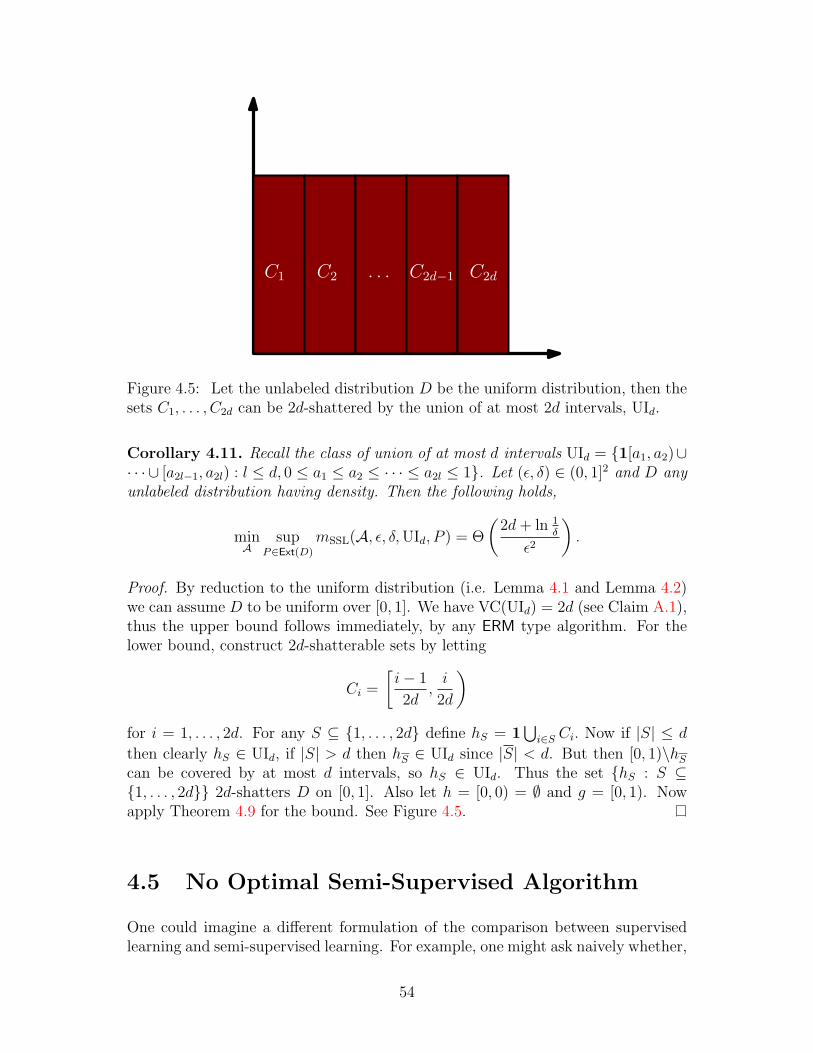
C1 C2 C2d−1 C2d. . .

Figure 4.5: Let the unlabeled distribution D be the uniform distribution, then thesets C1, . . . , C2d can be 2d-shattered by the union of at most 2d intervals, UId.

Corollary 4.11. Recall the class of union of at most d intervals UId = 1[a1, a2)∪· · · ∪ [a2l−1, a2l) : l ≤ d, 0 ≤ a1 ≤ a2 ≤ · · · ≤ a2l ≤ 1. Let (ε, δ) ∈ (0, 1]2 and D anyunlabeled distribution having density. Then the following holds,

minA

supP∈Ext(D)

mSSL(A, ε, δ,UId, P ) = Θ

(2d+ ln 1

δ

ε2

).

Proof. By reduction to the uniform distribution (i.e. Lemma 4.1 and Lemma 4.2)we can assume D to be uniform over [0, 1]. We have VC(UId) = 2d (see Claim A.1),thus the upper bound follows immediately, by any ERM type algorithm. For thelower bound, construct 2d-shatterable sets by letting

Ci =

[i− 1

2d,i

2d

)for i = 1, . . . , 2d. For any S ⊆ 1, . . . , 2d define hS = 1

⋃i∈S Ci. Now if |S| ≤ d

then clearly hS ∈ UId, if |S| > d then hS ∈ UId since |S| < d. But then [0, 1)\hScan be covered by at most d intervals, so hS ∈ UId. Thus the set hS : S ⊆1, . . . , 2d 2d-shatters D on [0, 1]. Also let h = [0, 0) = ∅ and g = [0, 1). Nowapply Theorem 4.9 for the bound. See Figure 4.5.

4.5 No Optimal Semi-Supervised Algorithm

One could imagine a different formulation of the comparison between supervisedlearning and semi-supervised learning. For example, one might ask naively whether,

54

for given class H, there is a semi-supervised algorithm A, such that for any super-vised algorithm B, and any sufficiently small ε, δ, on any data generating distri-bution P , the sample complexity of A is no larger than the sample complexity ofB. The answer to the question is easily seen to be negative, because for any Pthere exists a supervised learning algorithm BP that ignores the labeled examplesand simply outputs the hypothesis h ∈ H with minimum error ErP (h) (or eventhe Bayesian optimal classifier for P ). On P the sample complexity of BP is zero,unfortunately, on P ′, sufficiently different from P , the sample complexity of BP canbe infinite.

One might disregard algorithms such as BP and ask the same question as above,except that one quantifies over only the subset of algorithms that on any distribu-tion over X × 0, 1 have sample complexity that is distribution-free (e.g. poly-nomial in 1/ε and ln(1/δ)). That is, restricting oneself to learning algorithms (seeDefinition 2.5). The following theorem demonstrates that such restriction does nothelp and the answer to the question is still negative.

Theorem 4.12. Let H = 1(−∞, t] : t ∈ R be the class of thresholds overthe real line. For any unlabeled distribution D having density (with respect to theLebesgue measure), any semi-supervised algorithm A, any ε > 0 and δ ∈ (0, 1

2),

there exists a distribution P ∈ Ext(D) and a supervised learning algorithm B (seeDefinition 2.8) such that

mSSL(A, ε, δ,H, P ) > mSL(B, ε, δ,H, P ) .

Proof. Fix any A, D unlabeled distribution having density, and m. Let LeftERMbe the algorithm that chooses the right most positive point (for precise definition,see Equation 2.3). For any h ∈ H we also define algorithm

LeftERMh(S) :=

h if ErS(h) = 0

LeftERM(S) otherwise.

First, note that LeftERM = LeftERM1∅. Second, for any h, LeftERMh is an ERMparadigm (see Definition 2.11), and since VC(H) = 1, it is a learning algorithm.Third, clearly the sample complexity of LeftERMh on Dh is zero independently ofthe choice of ε and δ.

Theorem 4.5 shows that there exists a h ∈ H such that the sample complexityof A on Dh is positive, in fact, it is increasing as ε and δ approach zero. Thus,there exists a supervised algorithm B = LeftERMh with lower sample complexitythan A.

55

Chapter 5

Conclusion

This thesis has presented a fresh, new look at the theoretical underpinnings ofsemi-supervised learning. We proposed a novel, utopian model of semi-supervisedlearning where we assume the entire unlabeled distribution is given to the learnerand thus bypassing sampling issues of unlabeled training data.

Our analysis is concerned with the inherent limitations of semi-supervised learn-ing. In particular, we analyze the potential sample complexity gains in our utopianmodel of semi-supervised learning compared with that of supervised learning. Allthese analyses are done under what can be termed as the no-prior-knowledge set-ting, where no assumptions are made on the relationship between labels and theunlabeled data distribution.

Our main point is that semi-supervised learning cannot provide signifi-cant benefits over supervised learning, unless one is absolutely sure thatan assumption holds on the relationship between labels and the unlabeleddata distribution.

More technically, what we have proved is that for the class of thresholds (real-izable and agnostic) and union of intervals (agnostic) SSL cannot have better thana constant factor advantage in the sample complexity. We conjecture this to be amore general phenomenon that applies to any hypothesis class. Of course, this doesnot take into account the situation in which the learner makes SSL type assumptions(e.g. the cluster assumption) and is positive these assumptions hold. However, thedifficulty of verifying SSL assumptions or mathematically formalizing them is stilla wide open question. For example, we have illustrated counter-intuitive hazardsof learning under the cluster assumption.

Our work is the first in addressing the fundamental limitations of semi-supervisedlearning in a theoretical setting. We hope it is also a first step in bridging the gapbetween theory and practice of semi-supervised learning. There is still much futurework to be done and a few of them are given below.

56

5.1 Proving Conjectures 4.1 and 4.2

The main reason why one should believe the conjecture to be true (at least for therealizable case) is the algorithm of Kaariainen (2005). That is, a generalization ofMedianERM for arbitrary domains X where one finds the “centre” of the versionspace (i.e. consistent hypothesis on labeled data) where the (pseudo)-metric overthe hypothesis space is defined by the unlabeled distribution mass of the symmetricdifference of two hypotheses. Intuitively, supervised learning cannot find this centre,therefore in the worst-case it chooses a hypothesis on the “boundary” of the versionspace resulting in error at most the diameter of the version space whereas SSLachieves error at most the radius of the version space.

While we have shown the conjecture to be true for “smooth” unlabeled distri-butions (i.e. ones having a density function) for the class of thresholds in boththe realizable and agnostic settings, and union of intervals in the agnostic setting,it would be nice to prove it for unlabeled distributions that don’t have densities.These distributions include ones that are discrete, or a combination of discrete andcontinuous parts. For example, if the distribution is concentrated on one point, thebest SSL and SL algorithms do the same thing.

It would also be nice to prove a lower bound for supervised learning underthresholds in the realizable setting (for unlabeled distributions having density). Webelieve the lower bound should match the best known upper bound (e.g. LeftERM)of ln(1/δ)/ε within some negligible additive factor. This would imply that for anyunlabeled distribution having density, the SSL sample complexity is exactly twicebetter than SL sample complexity—without making SSL assumptions!

Of course, it will be quite interesting to prove the conjecture for classes inhigher dimensions. Unfortunately the reduction technique of Section 4.2 cannotbe easily extended for higher dimensions. For example, consider R2, and the map(x, y) 7→ (F1(x), F2(y)) where F1 and F2 are the CDFs for the x and y components,respectively. In order for this mapping to induce a uniform distribution over [0, 1]2,we need that F (x, y) = F1(x)F2(y) where F is the CDF over R2. In other words Fmust be a product distribution (having density). The class of axis-aligned rectangleswill retain its “shape” under this type of transformation, but not necessarily forlinear halfspaces (e.g. product Gaussian truncated beyond the unit square andhalfspace defined by y = 1 − x). However, we do not know of a lower bound onlearning axis-aligned rectangles with respect to the fixed uniform distribution overthe unit cube. Note that there are still transformations that will induce the uniformdistribution for non-product distributions, but it may disfigure the shape of say,axis-aligned rectangles.

5.2 Verifying SSL Assumptions

Our examples in Section 3.3 underscores the pitfalls when doing SSL with thecluster assumption. A natural question to consider is: is there’s a way to verify

57

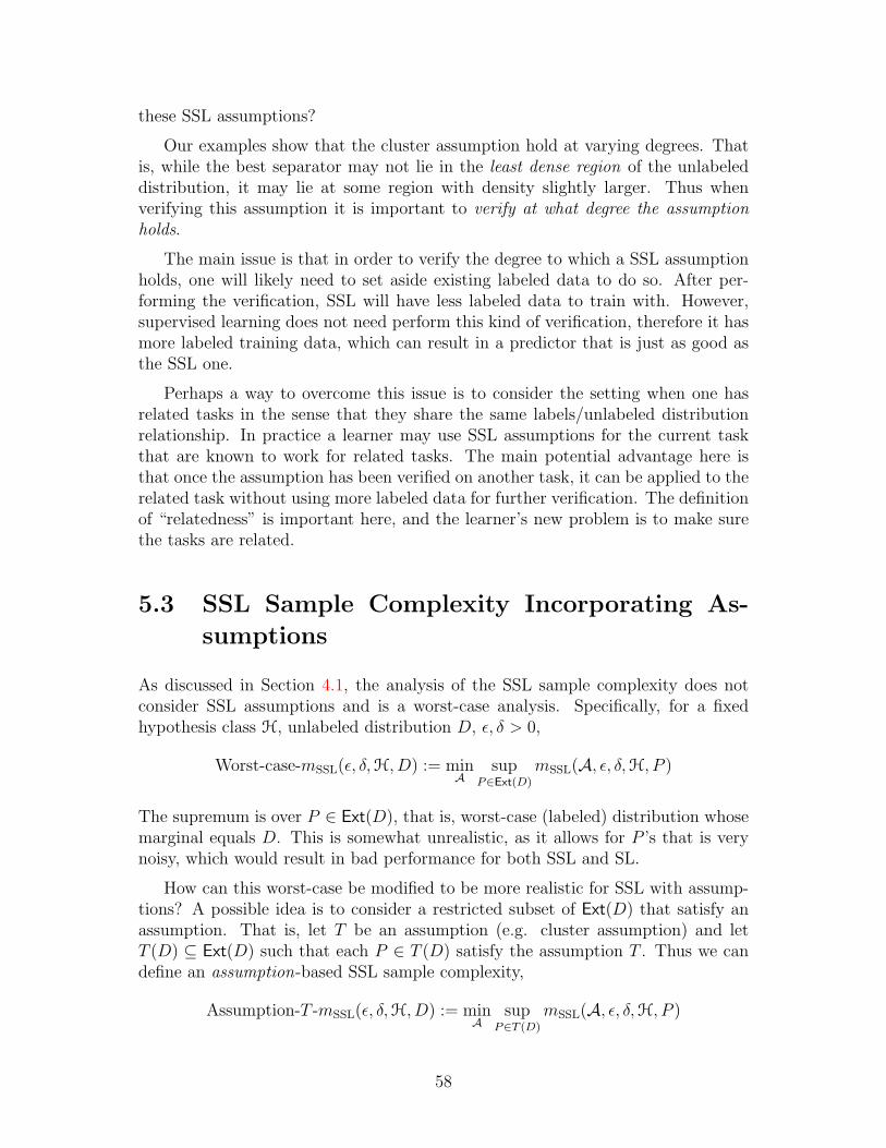
these SSL assumptions?

Our examples show that the cluster assumption hold at varying degrees. Thatis, while the best separator may not lie in the least dense region of the unlabeleddistribution, it may lie at some region with density slightly larger. Thus whenverifying this assumption it is important to verify at what degree the assumptionholds.

The main issue is that in order to verify the degree to which a SSL assumptionholds, one will likely need to set aside existing labeled data to do so. After per-forming the verification, SSL will have less labeled data to train with. However,supervised learning does not need perform this kind of verification, therefore it hasmore labeled training data, which can result in a predictor that is just as good asthe SSL one.

Perhaps a way to overcome this issue is to consider the setting when one hasrelated tasks in the sense that they share the same labels/unlabeled distributionrelationship. In practice a learner may use SSL assumptions for the current taskthat are known to work for related tasks. The main potential advantage here isthat once the assumption has been verified on another task, it can be applied to therelated task without using more labeled data for further verification. The definitionof “relatedness” is important here, and the learner’s new problem is to make surethe tasks are related.

5.3 SSL Sample Complexity Incorporating As-

sumptions

As discussed in Section 4.1, the analysis of the SSL sample complexity does notconsider SSL assumptions and is a worst-case analysis. Specifically, for a fixedhypothesis class H, unlabeled distribution D, ε, δ > 0,

Worst-case-mSSL(ε, δ,H, D) := minA

supP∈Ext(D)

mSSL(A, ε, δ,H, P )

The supremum is over P ∈ Ext(D), that is, worst-case (labeled) distribution whosemarginal equals D. This is somewhat unrealistic, as it allows for P ’s that is verynoisy, which would result in bad performance for both SSL and SL.

How can this worst-case be modified to be more realistic for SSL with assump-tions? A possible idea is to consider a restricted subset of Ext(D) that satisfy anassumption. That is, let T be an assumption (e.g. cluster assumption) and letT (D) ⊆ Ext(D) such that each P ∈ T (D) satisfy the assumption T . Thus we candefine an assumption-based SSL sample complexity,

Assumption-T -mSSL(ε, δ,H, D) := minA

supP∈T (D)

mSSL(A, ε, δ,H, P )

58

In the extreme case T (D) consists of only a single distribution and the (labeled)sample complexity is zero. For example, if T (D) consists of the distribution that isdefined by the lowest density linear separator (of D), then the task is to find thisseparator using only unlabeled data, since we know it has zero error. Clearly thisis too strong an assumption. On the other extreme, T consists of all Ext(D) whichprobably will not provide a significant advantage over supervised learning. Thus itis up to the learner to specify a T that takes into account this tradeoff.

59

APPENDICES

60

Appendix A

Examples of VC Dimension

This appendix shows some examples of the VC dimension of some basic hypothesisclasses. These classes include thresholds over the real line, finite union of intervalsand linear halfspaces in Euclidean space. In this thesis we make use of the VCdimension of the first two hypothesis classes, but the calculations for halfspaces isleft for didactical purposes.

Recall from Definition 2.10 that the Vapnik-Chervonenkis dimension of a hy-pothesis class H over input domain X is defined as

VC(H) := supd : ∃A ⊆ X , |A| = d, |H(A)| = 2d,where H(A) = h(A) : h ∈ H. That is, it is the size of the largest subset A of Xsuch that for any S ⊆ A, there is a hS ∈ H with set(hS) ∩ A = S.

A.1 Thresholds

The class of thresholds over the real line is defined as

H = 1(−∞, a] : a ∈ R.Figure A.1 shows an example hypothesis.

It is not hard to see that H can shatter one point, say 0, by the hypothesis1(−∞,−1] and 1(−∞, 1]. Let a, b ∈ R be any two points. Does there exist a tsuch that (−∞, t] ∩ a, b = b? No, because then t ≥ b which implies a must bein the intersection. Thus, VC(H) = 1.

t1(−∞, t] R1 0

Figure A.1: The class of thresholds consists of hypothesis that predicts 1 if a pointis less than the threshold, otherwise it predicts 0.

61

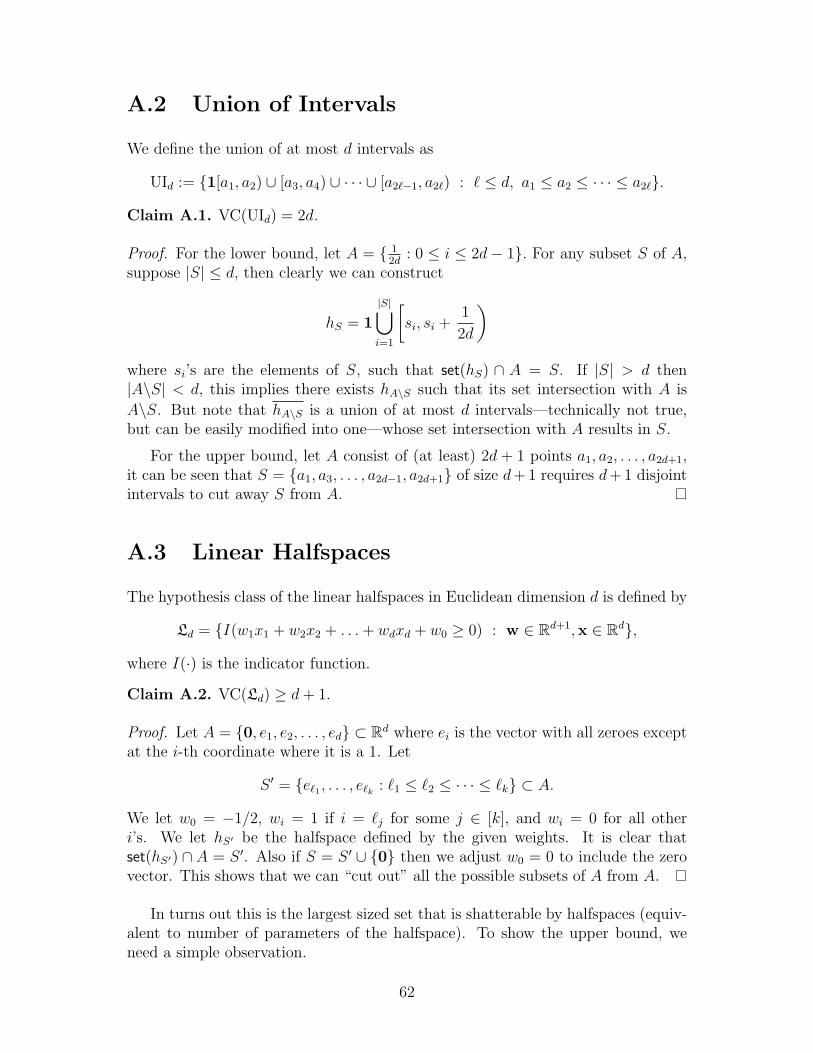
A.2 Union of Intervals

We define the union of at most d intervals as

UId := 1[a1, a2) ∪ [a3, a4) ∪ · · · ∪ [a2`−1, a2`) : ` ≤ d, a1 ≤ a2 ≤ · · · ≤ a2`.Claim A.1. VC(UId) = 2d.

Proof. For the lower bound, let A = 12d

: 0 ≤ i ≤ 2d− 1. For any subset S of A,suppose |S| ≤ d, then clearly we can construct

hS = 1

|S|⋃i=1

[si, si +

1

2d

)where si’s are the elements of S, such that set(hS) ∩ A = S. If |S| > d then|A\S| < d, this implies there exists hA\S such that its set intersection with A is

A\S. But note that hA\S is a union of at most d intervals—technically not true,but can be easily modified into one—whose set intersection with A results in S.

For the upper bound, let A consist of (at least) 2d + 1 points a1, a2, . . . , a2d+1,it can be seen that S = a1, a3, . . . , a2d−1, a2d+1 of size d+ 1 requires d+ 1 disjointintervals to cut away S from A.

A.3 Linear Halfspaces

The hypothesis class of the linear halfspaces in Euclidean dimension d is defined by

Ld = I(w1x1 + w2x2 + . . .+ wdxd + w0 ≥ 0) : w ∈ Rd+1,x ∈ Rd,where I(·) is the indicator function.

Claim A.2. VC(Ld) ≥ d+ 1.

Proof. Let A = 0, e1, e2, . . . , ed ⊂ Rd where ei is the vector with all zeroes exceptat the i-th coordinate where it is a 1. Let

S ′ = e`1 , . . . , e`k : `1 ≤ `2 ≤ · · · ≤ `k ⊂ A.

We let w0 = −1/2, wi = 1 if i = `j for some j ∈ [k], and wi = 0 for all otheri’s. We let hS′ be the halfspace defined by the given weights. It is clear thatset(hS′) ∩ A = S ′. Also if S = S ′ ∪ 0 then we adjust w0 = 0 to include the zerovector. This shows that we can “cut out” all the possible subsets of A from A.

In turns out this is the largest sized set that is shatterable by halfspaces (equiv-alent to number of parameters of the halfspace). To show the upper bound, weneed a simple observation.

62

Definition A.1. The convex hull of a finite1 set of points S = s1, . . . , sm ⊆ Rn

is

CH(S) =

λ1s1 + . . .+ λmsm : λ ≥ 0,

m∑i=1

λi = 1

.

Theorem A.3 (Radon). Let A = a1, . . . , ad+2 ⊂ Rd, then there exists two parti-tions of A, P,Q such that CH(P ) ∩ CH(Q) 6= ∅.

Proof. Consider the vectors A′ = (a1, 1), . . . , (ad+2, 1) ⊂ Rd+1 where an extra 1 isadded to the last coordinate. Basic linear algebra says that A′ is linearly dependent,that is, there exists constants c1, . . . , cd+2 ∈ R not all zero such that

c1(a1, 1) + c2(a2, 1) + . . .+ cd+2(ad+2, 1) = 0.

This implies these separate conditions,

d+2∑i=1

ciai = 0

d+2∑i=1

ci = 0

Let P = ai : ci > 0 and Q = A\P . By the above equations, the point

∑i:ai∈P

[ci∑

j:aj∈P cj

]ai =

∑i:ai∈Q

[ci∑

j:aj∈Q cj

]ai

is in both CH(P ) and CH(Q).

Corollary A.4. VC(Ld) = d+ 1.

Proof. The upper bound comes from Claim A.2. Given any A with at least d + 2points, we can find a partition of A, say P,Q such that their convex hulls do notintersect. A basic result in convex analysis says that a sufficient and necessarycondition for linear separability of two sets of points is that their convex hulls donot intersect. This means P and Q cannot be linearly separated, therefore neitherP nor Q can be “cut out” from A.

1The convex hull of any set (e.g. uncountable) can also be defined, but we will not need ithere.

63

References

Dana Angluin and Philip D. Laird. Learning from noisy examples. Machine Learn-ing, 2(4):343–370, 1987. 49

Martin Anthony and Peter L. Bartlett. Neural Network Learning: TheoreticalFoundations. Cambridge University Press, January 1999. 6, 16, 17, 49, 52, 53

Maria-Florina Balcan and Avrim Blum. A PAC-style model for learning from la-beled and unlabeled data. In Proceedings of 18th Annual Conference on LearningTheory, pages 111–126. Springer, 2005. 4, 22, 26

Maria-Florina Balcan and Avrim Blum. An augmented PAC model for semi-supervised learning. In Olivier Chapelle, Bernhard Scholkopf, and AlexanderZien, editors, Semi-Supervised Learning, chapter 21, pages 61–89. MIT Press,September 2006. 4, 22, 24

Shai Ben-David, Tyler Lu, and David Pal. Does unlabeled data provably help?worst-case analysis of the sample complexity of semi-supervised learning. InConference on Learning Theory, pages 33–44, 2008. 4, 37

Shai Ben-David, Tyler Lu, David Pal, and Miroslava Sotakova. Learning low densityseparators. In Proceedings of Artificial Intelligence and Statistics, 2009. Toappear. 33

Gyora M. Benedek and Alon Itai. Learnability with respect to fixed distributions.Theoretical Computer Science, 86(2):377–389, 1991. 22, 24, 25, 31

Patrick Billingsley. Probability and Measure. Wiley-Interscience, 3 edition, 1995. 6

Avrim Blum and Tom M. Mitchell. Combining labeled and unlabeled sata withco-training. In COLT, pages 92–100, 1998. 23

Avrim Blum and Ronald L. Rivest. Training a 3-node neural network is np-complete. In COLT, pages 9–18, 1988.

Anselm Blumer, Andrzej Ehrenfeucht, David Haussler, and Manfred K. Warmuth.Learnability and the vapnik-chervonenkis dimension. J. ACM, 36(4):929–965,1989. 8, 16

64

R. Bruce. Semi-supervised learning using prior probabilities and em. In IJCAIWorkshop on Text Learning: Beyond Supervision, August 2001. 23

Vittorio Castelli. The relative value of labeled and unlabeled samples in patternrecognition. PhD thesis, Stanford University, Stanford, CA, December 1994. 23

Vittorio Castelli and Thomas M. Cover. The relative value of labeled and unla-beled samples in pattern recognition with an unknown mixing parameter. IEEETransactions on Information Theory, 42(6):2102–2117, 1996. 23

Olivier Chapelle, Bernhard Scholkopf, and Alexander Zien, editors. Semi-SupervisedLearning. MIT Press, September 2006. 21, 23, 25, 26

Fabio Cozman and Ira Cohen. Risks of semi-supervised learning: How unlabeleddata can degrade performance of generative classifiers. In Olivier Chapelle, Bern-hard Scholkopf, and Alexander Zien, editors, Semi-Supervised Learning, chap-ter 4, pages 57–72. MIT Press, September 2006. 23

Sanjoy Dasgupta, Michael L. Littman, and David A. McAllester. Pac generalizationbounds for co-training. In NIPS, pages 375–382, 2001. 23

Luc Devroye, Laszlo Gyorfi, and Gabor Lugosi. A Probabilistic Theory of PatternRecognition (Stochastic Modelling and Applied Probability). Springer, February1997. ISBN 0387946187. 6

Andrzej Ehrenfeucht, David Haussler, Michael J. Kearns, and Leslie G. Valiant.A general lower bound on the number of examples needed for learning. Inf.Comput., 82(3):247–261, 1989. 16

Ran El-Yaniv and Dmitry Pechyony. Stable transductive learning. In COLT, pages35–49, 2006. 22

Ran El-Yaniv and Dmitry Pechyony. Transductive rademacher complexity and itsapplications. In COLT, pages 157–171, 2007. 21

Claudio Gentile and David P. Helmbold. Improved lower bounds for learning fromnoisy examples: and information-theoretic approach. In Proceedings of COLT1998, pages 104–115. ACM, 1998. 49

David Haussler. Decision theoretic generalizations of the pac model for neural netand other learning applications. Information and Computation, 100(1):78–150,1992. 6, 18

David Haussler. Sphere packing numbers for subsets of the boolean n-cube withbounded vapnik-chervonenkis dimension. Journal of Combinatorial Theory, Se-ries A, 69(2):217–232, 1995. 14

Thorsten Joachims. Transductive inference for text classification using supportvector machines. In ICML, pages 200–209, 1999. 23, 26

65

Matti Kaariainen. Generalization error bounds using unlabeled data. In Proceedingsof COLT 2005, pages 127–142. Springer, 2005. vii, 4, 22, 25, 30, 40, 41, 57

Michael J. Kearns and Umesh V. Vazirani. An introduction to computational learn-ing theory. MIT Press, Cambridge, MA, USA, 1994. ISBN 0-262-11193-4. 6,42

Michael J. Kearns, Robert E. Schapire, and Linda M. Sellie. Toward efficientagnostic learning. In COLT ’92: Proceedings of the fifth annual workshop onComputational learning theory, pages 341–352, New York, NY, USA, 1992. ACM.ISBN 0-89791-497-X. doi: http://doi.acm.org/10.1145/130385.130424. 6, 18

Michael J. Kearns, Robert E. Schapire, and Linda M. Sellie. Toward efficientagnostic learning. Machine Learning, 17(2):115–141, 1994. 6, 18

Philip M. Long. On the sample complexity of PAC learning half-spaces against theuniform distribution. IEEE Transactions on Neural Networks, 6(6):1556–1559,1995.

Philip M. Long. An upper bound on the sample complexity of PAC-learning half-spaces with respect to the uniform distribution. Information Processing Letters,87(5):229–234, 2003.

Joel Ratsaby and Santosh S. Venkatesh. Learning from a mixture of labeled andunlabeled examples with parametric side information. In COLT, pages 412–417,1995. 23

Philippe Rigollet. Generalization error bounds in semi-supervised classificationunder the cluster assumption. Journal of Machine Learning Research, 8:1369–1392, 2007. 27

A. Singh, R. Nowak, and X. Zhu. Unlabeled data: Now it helps, now it doesn’t. InNIPS, 2008.

F. Oles T. Zhang. A probability analysis on the value of unlabeled data for classi-fication problems. In ICML, pages 1191–1198, 2000. 23

M. Talagrand. Sharper bounds for gaussian and empirical processes. Annals ofProbability, 22(28-76), 1994. 14

Leslie G. Valiant. A theory of the learnable. Communications of the ACM, 27(11):1134–1142, 1984. 3, 4, 6, 18

Vladimir Vapnik and Alexei Chervonenkis. On the uniform convergence of relativefrequencies to their probabilities. Theoretical Probability and Its Applications, 2:264–280, 1971. 4, 6, 13, 14

Vladimir Vapnik and Alexei Chervonenkis. Theory of Pattern Recognition. Nauka,Moscow, 1974. in Russian. 16

66

Vladimir N. Vapnik. Statistical Learning Theory. Wiley-Interscience, September1998. 6

Vladimir N. Vapnik. Transductive inference and semi-supervised learning. In OlivierChapelle, Bernhard Scholkopf, and Alexander Zien, editors, Semi-SupervisedLearning, chapter 24, pages 453–472. MIT Press, September 2006. 4, 21

Xiaojin Zhu. Semi-supervised learning with graphs. PhD thesis, Carnegie MellonUniversity, 2005.

Xiaojin Zhu. Semi-supervised learning literature survey. Technical Report 1530,Computer Science, University of Wisconsin Madison, 2008. 2

67