FUNCTIONS AND MODELSFUNCTIONS AND MODELS

1

In this section, we assume that you

have access to a graphing calculator

or a computer with graphing software.

FUNCTIONS AND MODELS

1.4Graphing Calculators

and Computers

In this section, we will learn about:

The advantages and disadvantages of

using graphing calculators and computers.

FUNCTIONS AND MODELS

In this section, we:

Will see that the use of a graphing device enables us to graph more complicated functions and to solve more complex problems than would otherwise be possible.

Point out some of the pitfalls that can occur with these machines.

GRAPHING CALCULATORS AND COMPUTERS

Graphing calculators and computers

can give very accurate graphs of

functions.

However, we will see in Chapter 4 that, only through the use of calculus, can we be sure that we have uncovered all the interesting aspects of a graph.

GRAPHING CALCULATORS AND COMPUTERS

A graphing calculator or computer displays a rectangular portion of the graph of a function in a display window or viewing screen.

This is referred to as a viewing rectangle.

VIEWING RECTANGLE

The default screen often gives an

incomplete or misleading picture.

So, it is important to choose the viewing

rectangle with care.

VIEWING RECTANGLE

If we choose the x-values to range from a

minimum value of Xmin = a to a maximum

value of Xmax = b and the y-values to range

from a minimum of Ymin = c to a maximum of

Ymax = d, then the visible portion of the

graph lies in the rectangle

[ , ] [ , ] ( , ) | ,a b c d x y a x b c y d

VIEWING RECTANGLE

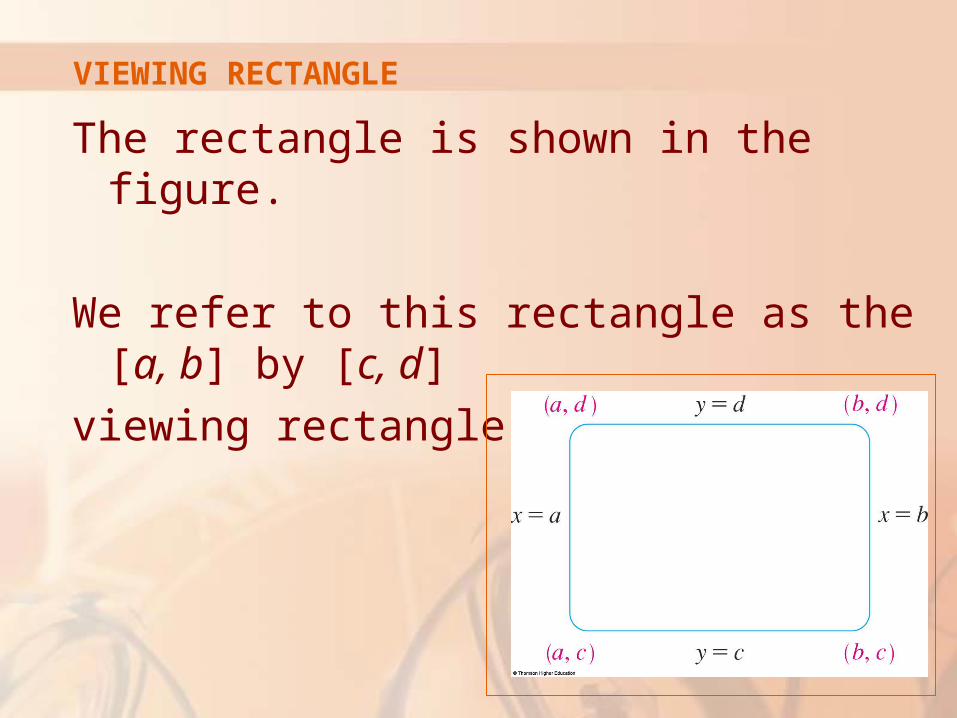
The rectangle is shown in the figure.

We refer to this rectangle as the [a, b] by [c, d]

viewing rectangle.

VIEWING RECTANGLE

The machine draws the graph of

a function f much as you would.

It plots points of the form (x, f(x)) for a certain number of equally spaced values of x between a and b.

If an x-value is not in the domain of f, or if f(x) lies outside the viewing rectangle, it moves on to the next x-value.

The machine connects each point to the preceding plotted point to form a representation of the graph of f.

GRAPHING

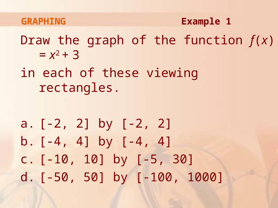
Draw the graph of the function f(x) = x2 + 3

in each of these viewing rectangles.

a. [-2, 2] by [-2, 2]

b. [-4, 4] by [-4, 4]

c. [-10, 10] by [-5, 30]

d. [-50, 50] by [-100, 1000]

Example 1GRAPHING

We select the range by setting Xmin = -2,

Xmax = 2,Ymin = -2 and Ymax = 2.

The resulting graph is shown. The display window is blank.

Example 1 aGRAPHING

A moment’s thought provides the explanation.

Notice that for all x, so for all x. Thus, the range of the function

is . This means that

the graph of f lies entirely outside the viewing rectangle by [-2, 2] by [-2, 2].

2 0x 2 3 3x 2( ) 3f x x

[3, )

Example 1 aGRAPHING

The graphs for the viewing rectangles

in (b), (c), and (d) are shown. Observe that we get a more complete picture

in (c) and (d). However, in (d), it is not clear that the y-intercept

is 3.

Example 1 b, c, dGRAPHING

From Example 1, we see that the choiceof a viewing rectangle can make a bigdifference in the appearance of a graph.

Often, it’s necessary to change to a larger viewing rectangle to obtain a more complete picture—a more global view—of the graph.

GRAPHING

In the next example, we see that knowledge

of the domain and range of a function

sometimes provides us with enough

information to select a good viewing rectangle.

GRAPHING

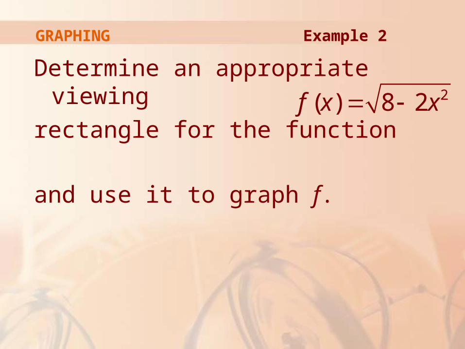
Determine an appropriate viewing

rectangle for the function

and use it to graph f.

2( ) 8 2f x x

Example 2GRAPHING

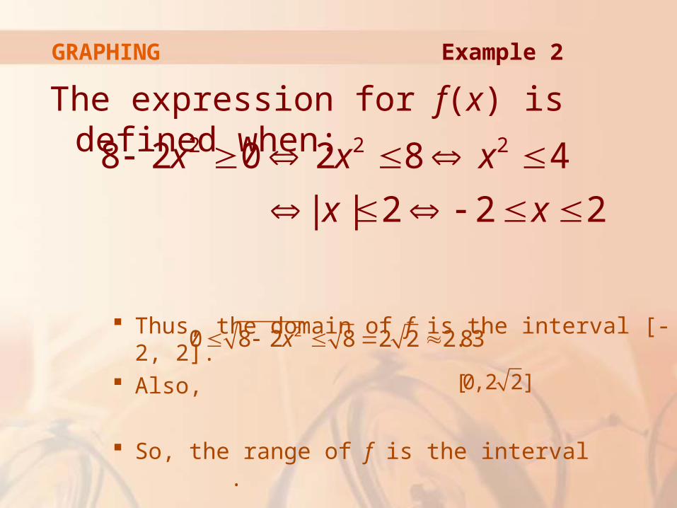
The expression for f(x) is defined when:

Thus, the domain of f is the interval [-2, 2]. Also,

So, the range of f is the interval .

2 2 28 2 0 2 8 4

| | 2 2 2

x x x

x x

20 8 2 8 2 2 2.83x

[0, 2 2]

Example 2GRAPHING

We choose the viewing rectangle so that

the x-interval is somewhat larger than

the domain and the y-interval is larger than

the range. Taking the viewing

rectangle to be [-3, 3] by [-1, 4], we get the graph shown here.

Example 2GRAPHING

Graph the function .

Here, the domain is , the set of all real numbers. That doesn’t help us choose a viewing rectangle.

3 150y x x Example 3GRAPHING

Let’s experiment.

If we start with the viewing rectangle [-5, 5] by [-5, 5], we get the graph shown here.

It appears blank. Actually, it is so nearly

vertical that it blends in with the y-axis.

GRAPHING Example 3

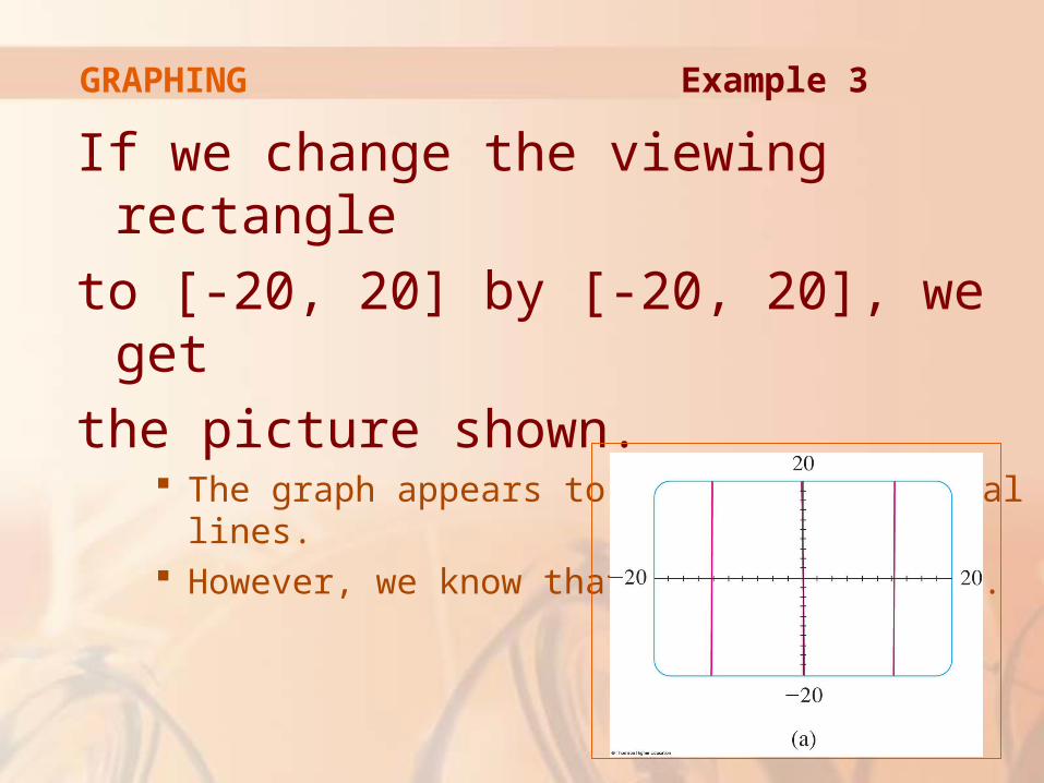
If we change the viewing rectangle

to [-20, 20] by [-20, 20], we get

the picture shown. The graph appears to consist of vertical lines. However, we know that can’t be correct.

Example 3GRAPHING

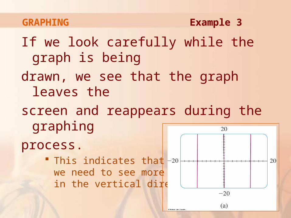
If we look carefully while the graph is being

drawn, we see that the graph leaves the

screen and reappears during the graphing

process. This indicates that

we need to see more in the vertical direction.

Example 3GRAPHING

So, we change the viewing rectangle to

[-20, 20] by [-500, 500].

The resulting graph is shown.

It still doesn’t quite reveal all the main features of the function.

Example 3GRAPHING

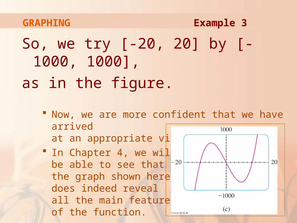
So, we try [-20, 20] by [-1000, 1000],

as in the figure.

Now, we are more confident that we have arrived at an appropriate viewing rectangle.

In Chapter 4, we will be able to see that the graph shown here does indeed reveal all the main features of the function.

GRAPHING Example 3

Graph the function

f(x) = sin 50x

in an appropriate viewing rectangle.

GRAPHING Example 4

The figure shows the graph of f produced by

a graphing calculator using the viewing

rectangle [-12, 12] by [-1.5, 1.5].

At first glance, the graph appears to be reasonable.

Example 4GRAPHING

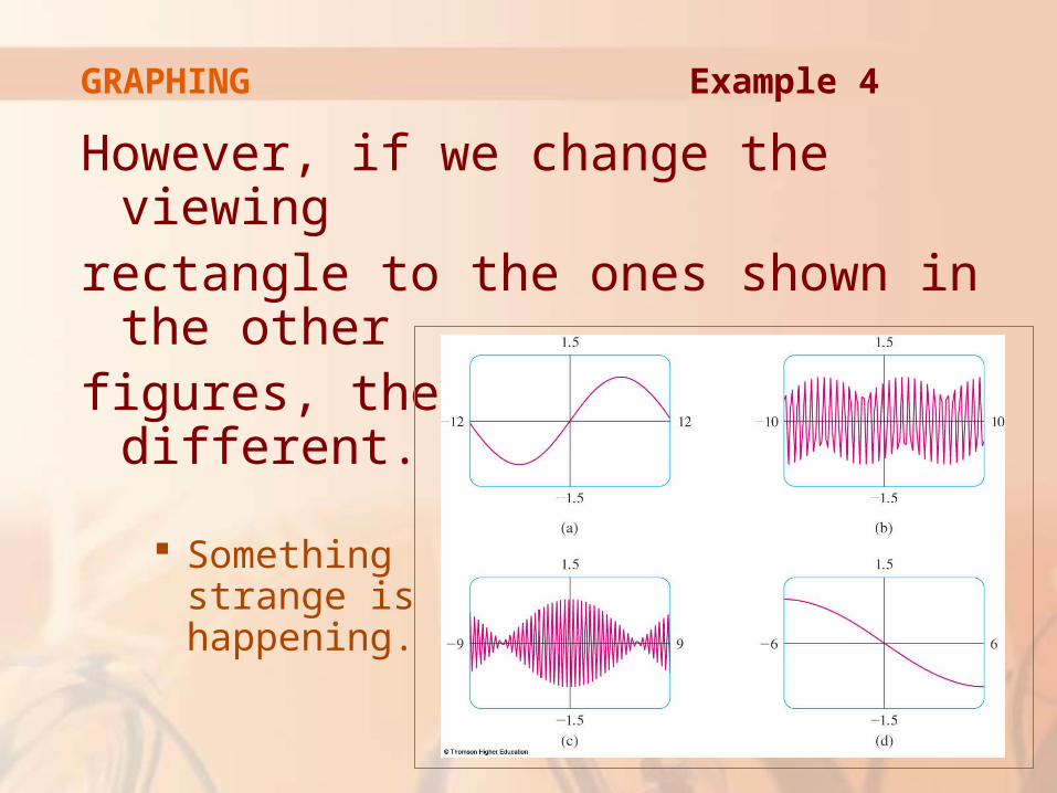
However, if we change the viewing rectangle to the ones shown in the other figures, the graphs look very different.

Something strange is happening.

Example 4GRAPHING

To explain the big differences in appearance

of those graphs and to find an appropriate

viewing rectangle, we need to find the period

of the function y = sin 50x.

GRAPHING Example 4

We know that the function y = sin x has

period and the graph of y = sin 50x

is compressed horizontally by a factor of 50.

So, the period of y = sin 50x is:

This suggests that we should deal only with small values of x to show just a few oscillations of the graph.

2

20.126

50 25

Example 4GRAPHING

If we choose the viewing rectangle

[-0.25, 0.25] by [-1.5, 1.5], we get

the graph shown here.

Example 4GRAPHING

Now, we see what went wrong in

the earlier graphs. The oscillations of y = sin 50x are so rapid that,

when the calculator plots points and joins them, it misses most of the maximum and minimum points.

Thus, it gives a very misleading impression of the graph.

Example 4GRAPHING

We have seen that the use of an

inappropriate viewing rectangle can

give a misleading impression of

the graph of a function.

GRAPHING

GRAPHING

In Examples 1 and 3, we solved the

problem by changing to a larger viewing

rectangle.

In Example 4, we had to make the

rectangle smaller.

In the next example, we look at a

function for which there is no single

viewing rectangle that reveals the true

shape of the graph.

GRAPHING

Graph the function

1100( ) sin cos 100f x x x

Example 5GRAPHING

The figure shows the graph of f produced by

a graphing calculator with viewing rectangle

[-6.5, 6.5] by [-1.5, 1.5].

It looks much like the graph of y = sin x, but perhaps with some bumps attached.

GRAPHING Example 5

If we zoom in to the viewing rectangle

[-0.1, 0.1] by [-0.1, 0.1], we can see much

more clearly the shape of these bumps—as

in the other figure.

Example 5GRAPHING

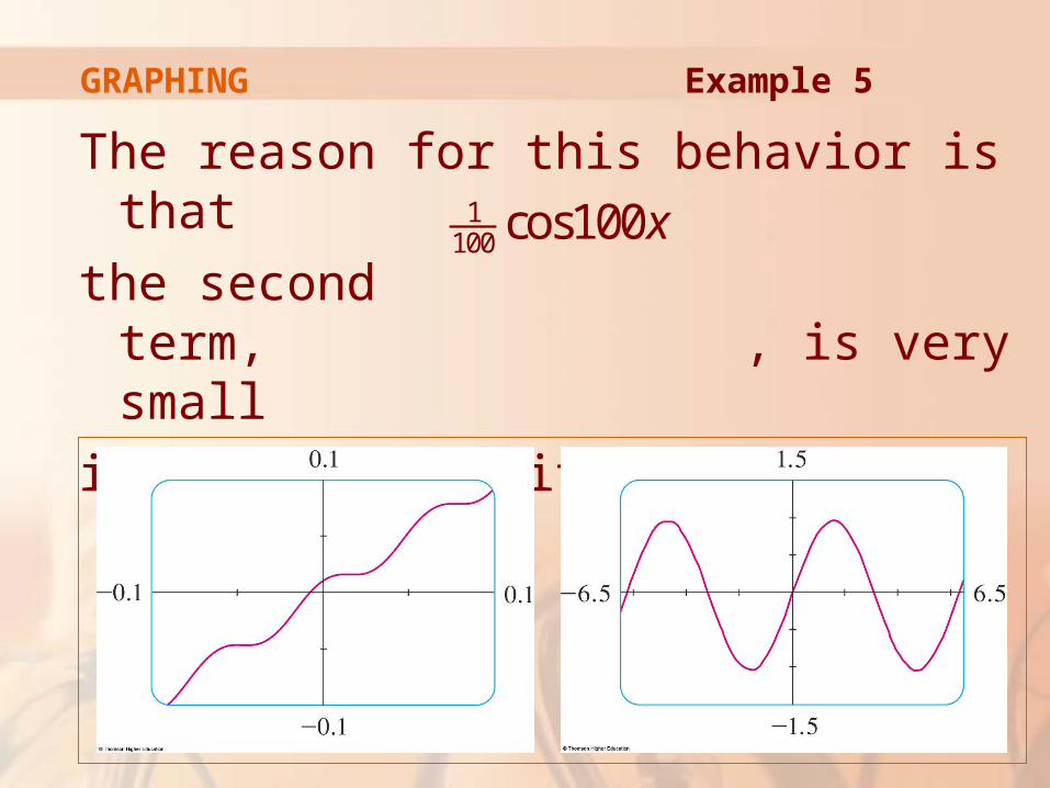
The reason for this behavior is that

the second term, , is very small

in comparison with the first term, sin x.

GRAPHING Example 5

1100 cos100x

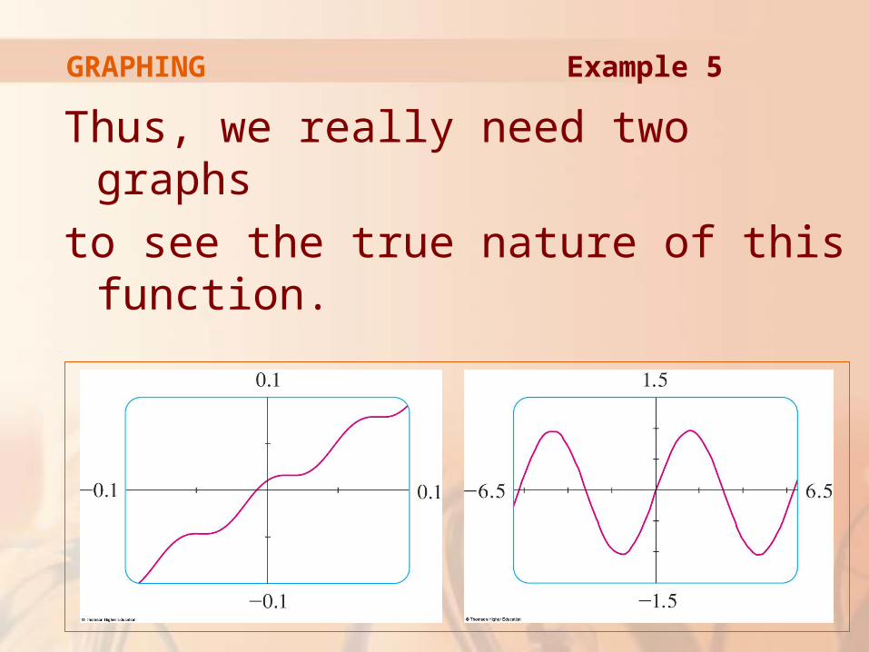
Thus, we really need two graphs

to see the true nature of this function.

GRAPHING Example 5

Draw the graph of the

function

GRAPHING Example 6

1

1y

x

The figure shows the graph produced

by a graphing calculator with viewing

rectangle [-9, 9] by [-9, 9].

Example 6GRAPHING

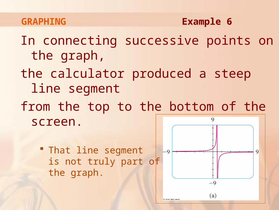
In connecting successive points on the graph,

the calculator produced a steep line segment

from the top to the bottom of the screen.

That line segment is not truly part of the graph.

GRAPHING Example 6

Notice that the domain of the function y = 1/(1 – x) is {x | x ≠ 1}.

Example 6GRAPHING

We can eliminate the extraneous

near-vertical line by experimenting

with a change of scale.

GRAPHING Example 6

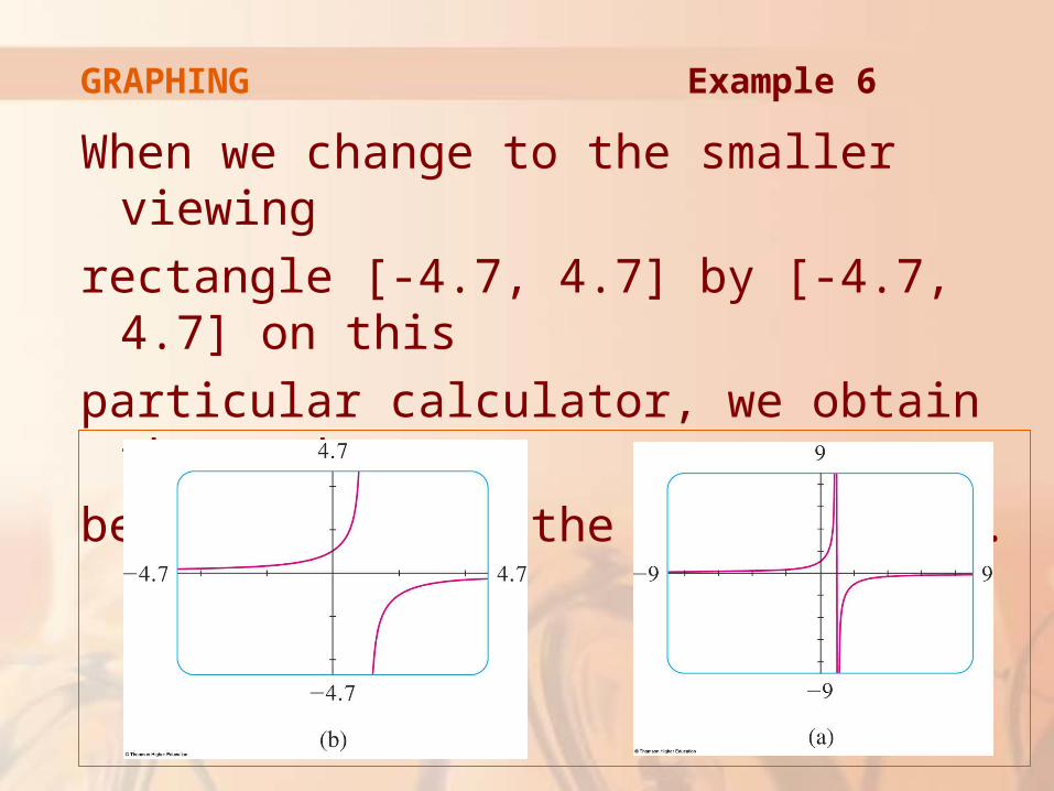
When we change to the smaller viewing

rectangle [-4.7, 4.7] by [-4.7, 4.7] on this

particular calculator, we obtain the much

better graph in the other figure.

Example 6GRAPHING

Graph the function .

Some graphing devices display the graph shown in the first figure.

However, others produce a graph like that in the second figure.

3y xExample 7GRAPHING

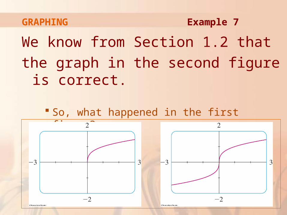
We know from Section 1.2 that

the graph in the second figure is correct.

So, what happened in the first figure?

GRAPHING Example 7

Here’s the explanation.

Some machines compute the cube root of using a logarithm—which is not defined if x is negative.

So, only the right half of the graph is produced.

GRAPHING Example 7

You should experiment with your

own machine to see which of these

two graphs is produced.

GRAPHING Example 7

If you get the graph in the first figure,

you can obtain the correct picture by

graphing the function

This function is equal to (except when x = 0).

1/3( ) | || |

xf x x

x

3 x

Example 7GRAPHING

To understand how the expression for

a function relates to its graph, it’s helpful

to graph a family of functions.

This is a collection of functions whose equations are related.

GRAPHING

In the next example, we graph

members of a family of cubic

polynomials.

GRAPHING

Graph the function y = x3 + cx for

various values of the number c.

How does the graph change when c

is changed?

Example 8GRAPHING

The graphs of y = x3 + cx for c = 2, 1, 0,

-1, and -2 are displayed.

We see that, for positive values of c, the graph increases from left to right with no maximum or minimum points (peaks or valleys).

GRAPHING Example 8

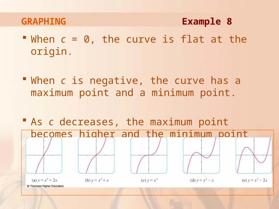
When c = 0, the curve is flat at the origin.

When c is negative, the curve has a maximum point and a minimum point.

As c decreases, the maximum point becomes higher and the minimum point lower.

Example 8GRAPHING

Find the solution of the equation

cos x = x correct to two decimal

places.

The solutions of the equation cos x = x are the x-coordinates of the points of intersection of the curves y = cos x and y = x.

Example 9GRAPHING

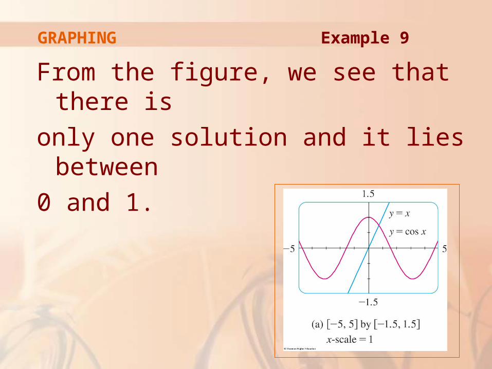
From the figure, we see that there is

only one solution and it lies between

0 and 1.

Example 9GRAPHING

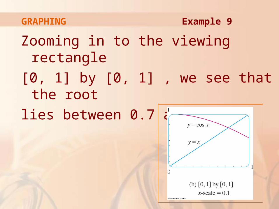
Zooming in to the viewing rectangle

[0, 1] by [0, 1] , we see that the root

lies between 0.7 and 0.8

GRAPHING Example 9

So, we zoom in further to the viewing

rectangle [0.7, 0.8] by [0.7, 0.8]

Example 9GRAPHING

By moving the cursor to the intersection point

of the two curves—or by inspection and

the fact that the x-scale is 0.01—we see that

the solution of the equation is about 0.74

Many calculators have a built-in intersection feature.

GRAPHING Example 9