FUNCTIONALANALYSIS - Departmentsrgelca/FUNCTANAL.pdf · Lecture notes by R˘azvan Gelca. 2. ......
89
FUNCTIONAL ANALYSIS Lecture notes by R˘azvan Gelca
Transcript of FUNCTIONALANALYSIS - Departmentsrgelca/FUNCTANAL.pdf · Lecture notes by R˘azvan Gelca. 2. ......

FUNCTIONAL ANALYSIS
Lecture notes by Razvan Gelca

2

Contents
1 Topological Vector Spaces 5
1.1 What is functional analysis? . . . . . . . . . . . . . . . . . . . . . . . . . . . 51.2 The definition of topological vector spaces . . . . . . . . . . . . . . . . . . . 51.3 Basic properties of topological vector spaces . . . . . . . . . . . . . . . . . . 71.4 Hilbert spaces . . . . . . . . . . . . . . . . . . . . . . . . . . . . . . . . . . . 81.5 Banach spaces . . . . . . . . . . . . . . . . . . . . . . . . . . . . . . . . . . . 161.6 Frechet spaces . . . . . . . . . . . . . . . . . . . . . . . . . . . . . . . . . . . 18
1.6.1 Seminorms . . . . . . . . . . . . . . . . . . . . . . . . . . . . . . . . . 181.6.2 Frechet spaces . . . . . . . . . . . . . . . . . . . . . . . . . . . . . . . 20
2 Linear Functionals 23
2.1 The Riesz representation theorem . . . . . . . . . . . . . . . . . . . . . . . . 232.2 The Riesz Representation Theorem for Hilbert spaces . . . . . . . . . . . . . 272.3 The Hahn-Banach Theorems . . . . . . . . . . . . . . . . . . . . . . . . . . . 282.4 A few results about convex sets . . . . . . . . . . . . . . . . . . . . . . . . . 312.5 The dual of a topological vector space . . . . . . . . . . . . . . . . . . . . . . 34
2.5.1 The weak∗-topology . . . . . . . . . . . . . . . . . . . . . . . . . . . . 342.5.2 The dual of a normed vector space . . . . . . . . . . . . . . . . . . . 36
3 Fundamental Results about Bounded Linear Operators 41
3.1 Continuous linear operators . . . . . . . . . . . . . . . . . . . . . . . . . . . 413.1.1 The case of general topological vector spaces . . . . . . . . . . . . . . 41
3.2 The three fundamental theorems . . . . . . . . . . . . . . . . . . . . . . . . 423.2.1 Baire category . . . . . . . . . . . . . . . . . . . . . . . . . . . . . . . 423.2.2 Bounded linear operators on Banach spaces . . . . . . . . . . . . . . 42
3.3 The adjoint of an operator between Banach spaces . . . . . . . . . . . . . . . 473.4 The adjoint of an operator on a Hilbert space . . . . . . . . . . . . . . . . . 503.5 The heat equation . . . . . . . . . . . . . . . . . . . . . . . . . . . . . . . . 56
4 Banach Algebra Techniques in Operator Theory 59
4.1 Banach algebras . . . . . . . . . . . . . . . . . . . . . . . . . . . . . . . . . . 594.2 Spectral theory for Banach algebras . . . . . . . . . . . . . . . . . . . . . . . 614.3 Functional calculus with holomorphic functions . . . . . . . . . . . . . . . . 644.4 Compact operators, Fredholm operators . . . . . . . . . . . . . . . . . . . . 674.5 The Gelfand transform . . . . . . . . . . . . . . . . . . . . . . . . . . . . . . 69
3

4 CONTENTS
5 C∗ algebras 73
5.1 The definition of C∗-algebras . . . . . . . . . . . . . . . . . . . . . . . . . . . 735.2 Commutative C∗-algebras . . . . . . . . . . . . . . . . . . . . . . . . . . . . 755.3 C∗-algebras as algebras of operators . . . . . . . . . . . . . . . . . . . . . . . 765.4 Functional calculus for normal operators . . . . . . . . . . . . . . . . . . . . 77
6 Topics presented by the students 87
A Background results 89
A.1 Zorn’s lemma . . . . . . . . . . . . . . . . . . . . . . . . . . . . . . . . . . . 89

Chapter 1
Topological Vector Spaces
1.1 What is functional analysis?
Functional analysis is the study of vector spaces endowed with a topology, and of the mapsbetween such spaces.
Linear algebra in infinite dimensional spaces.
It is a field of mathematics where linear algebra and geometry/topology meet.
Origins and applications
• The study of spaces of functions (continuous, integrable) and of transformations be-tween them (differential operators, Fourier transform).
• The study of differential and integral equations (understanding the solution set).
• Quantum mechanics (the Heisenberg formalism).
1.2 The definition of topological vector spaces
The field of scalars will always be either R or C, the default being C.
Definition. A vector space over C (or R) is a set V endowed with an addition and a scalarmultiplication with the following properties
• to every pair of vectors x, y ∈ V corresponds a vector x+ y ∈ V such thatx+ y = y + x for all x, yx+ (y + z) = (x+ y) + z for all x, y, zthere is a unique vector 0 ∈ V such that x+ 0 = 0 + x = x for all xfor each x ∈ V there is −x ∈ V such that x+ (−x) = 0.
5

6 CHAPTER 1. TOPOLOGICAL VECTOR SPACES
• for every α ∈ C (respectively R) and x ∈ V , there is αx ∈ V such that1x = x for all xα(βx) = (αβ)x for all α, β, xα(x+ y) = αx+ αy, (α + β)x = αx+ βx.
A set C ∈ V is called convex if tC + (1− t)C ⊂ C for every t ∈ [0, 1].A set B ⊂ V is called balanced if for every scalar α with |α| ≤ 1, αB ⊂ B.
Definition. If V and W are vector spaces, a map T : V → W is called a linear map (orlinear operator) if for every scalars α and β and every vectors x, y ∈ V ,
T (αx+ βy) = αTx+ βTy.
Definition. A topological space is a set X together with a collection T of subsets of X withthe following properties
• ∅ and X are in T
• The union of arbitrarily many sets from T is in T
• The intersection of finitely many sets from T is in T .
The sets in T are called open.
If X and Y are topological spaces, the X × Y is a topological space in a natural way, bydefining the open sets in X × Y to be arbitrary unions of sets of the form U1 ×U2 where U1
is open in X and U2 is open in Y .
Definition. A map f : X → Y is called continuous if for every open set U ∈ Y , the setf−1(U) is open in X.
A map is called a homeomorphism if it is invertible and both the map and its inverse arecontinuous. A topological space X is called Hausdorff if for every x, y ∈ X, there are opensets U1 and U2 such that x ∈ U1, y ∈ U2 and U1 ∩ U2 = ∅.
A neighborhood of x is an open set containing x. A system of neighborhoods of x is afamily of neighborhoods of x such that for every neighborhood of x there is a member of thisfamily inside it.
A subset C ∈ X is closed if X\C is open. A subset K ∈ X is called compact if everycovering of K by open sets has a finite subcover. The closure of a set is the smallest closedset that contains it. If A is a set then A denotes its closure. The interior of a set is thelargest open set contained in it. We denote by int(A) the interior of A.
Definition. A topological vector space over the field K (which is either C or R) is a vectorspace X endowed with a topology such that every point is closed and with the property thatboth addition and scalar multiplication,
+ : X ×X → X and · : K ×X → X,
are continuous.

1.3. BASIC PROPERTIES OF TOPOLOGICAL VECTOR SPACES 7
Example. Rn is an example of a finite dimensional topological vector space, while C([0, 1])is an example of an infinite dimensional vector space.
A subset E of a topological vector space is called bounded if for every neighborhood Uof 0 there is a number s > 0 such that E ⊂ tU for every t > s.
A topological vector space is called locally convex if every point has a system of neigh-borhoods that are convex.
1.3 Basic properties of topological vector spaces
Let X be a topological vector space.
Proposition 1.3.1. For every a ∈ X, the translation operator x 7→ x + a is a homeomor-phism.
As a corollary, the topology on X is completely determined by a system of neighborhoodsat the origin; the topology is translation invariant.
Proposition 1.3.2. Let W be a neighborhood of 0 in X. Then there is a neighborhood Uof 0 which is symmetric (U = −U) such that U + U ⊂ W .
Proof. Because addition is continuous there are open neighborhoods of 0, U1 and U2, suchthat U1 + U2 ⊂ W . Choose U = U1 ∩ U2 ∩ (−U1) ∩ (−U2).
Proposition 1.3.3. Suppose K is a compact and C is a closed subset of X such thatK ∩ C = ∅. Then there is a neighborhood U of 0 such that
(K + U) ∩ (C + U) = ∅.
Proof. Applying twice Proposition 1.3.2 twice we we deduce that for every neighborhood Wof 0 there is an open symmetric neighborhood U of 0 such that U + U + U +U ⊂ W . Sincethe topology is translation invariant, it means that for every neighborhood W of a point xthere is an open symmetric neighborhood of 0, Ux, such that x+ Ux + Ux + Ux + Ux ⊂ W .
Now let x ∈K and W = X\C. Then x + Ux + Ux + Ux + Ux ⊂ X\C, and since Ux issymmetric, (x+ Ux + Ux) ∩ (C + Ux + Ux) = ∅.
Since K is compact, there are finitely many points x1, x2, . . . , xk such that K ⊂ (x1 +Ux1
) ∪ (x2 + Ux2) ∪ · · · (xk + Uxk
). Set U = Ux1∩ Ux2
∩ · · · ∩ Uxk. Then
K + U ⊂ (x1 + Ux1) + U) ∪ (x2 + Ux2
+ U) ∪ · · · ∪ (xk + Uxk+ U)
⊂ (x1 + Ux1+ Ux1
) ∪ (x2 + Ux2+ Ux2
) ∪ · · · ∪ (xk + Uxk+ Uxk
)
⊂ X\[(C + Ux1+ Ux1
) ∩ · · · ∩ (C + Uxk+ Uxk
) ⊂ X\(C + U)],
and we are done.
Corollary 1.3.1. Given a system of neighborhoods of a point, every member of it containsthe closure of some other member.
Proof. Set K equal to a point.

8 CHAPTER 1. TOPOLOGICAL VECTOR SPACES
Corollary 1.3.2. Every topological vector space is Hausdorff.
Proof. Let K and C be points.
Proposition 1.3.4. Let X be a topological vector space.a) If A ⊂ X then A = ∩(A+ U), where U runs through all neighborhoods of 0.b) If A ⊂ X and B ⊂ X, then A+ B ⊂ A+ B.c) If Y is a subspace of X, then so is Y .d) If C is convex, then so are C and int(C).e) If B is a balanced subset of X, then so is B, if 0 ∈ int(B), then int(B) is balanced.f) If E is bounded, then so is E.
Theorem 1.3.1. In a topological vector space X,a) every neighborhood of 0 contains a balanced neighborhood of 0,b) every convex neighborhood of 0 contains a balanced convex neighborhood of 0.
Proof. a) Because multiplication is continuous, for every neighborhood W of 0 there are anumber δ > 0 and a neighborhood U of 0 such that αU ⊂ W for all α such that |α| < δ.The balanced neighborhood is the union of all αU for |α| < δ.
b) Let W be a convex neighborhood of 0. Let A = ∩αW , where α ranges over allscalars of absolute value 1. Let U be a balanced neighborhood of 0 contained in W . ThenU = αU ⊂ αW , so U ⊂ A. It follows that int(A) 6= ∅. Because A is the intersection ofconvex sets, it is convex, and hence so is int(A). Let us show that A is balanced, which wouldimply that int(A) is balanced as well. Every number α such that |α| < 1 can be written asα = rβ with 0 ≤ r ≤ 1 and |β| = 1. If x ∈ A, then βx ∈ A and so (1 − r)0 + rβx = αx isalso in A by convexity. This proves that A is balanced.
Proposition 1.3.5. a) Suppose U is a neighborhood of 0. If rn is a sequence of positivenumbers with limn→∞ rn = ∞, then
X = ∪∞n=1rnU.
b) If δn is a sequence of positive numbers converging to 0, and if U is bounded, then δnU ,n ≥ 0 is a system of neighborhoods at 0.
Proof. a) Let x ∈ X. Since α 7→ αx is continuous, there is n such that 1/rnx ∈ U . Hencex ∈ rnU .
b) Let W be a neighborhood of 0. Then there is s such that if t > s then U ⊂ tW .Choose δn < 1/s.
Corollary 1.3.3. Every compact set is bounded.
1.4 Hilbert spaces
Let V be a linear space (real or complex). An inner product on V is a function
〈 , 〉 : V × V → C
that sastisfies the following properties

1.4. HILBERT SPACES 9
• 〈y, x〉 = 〈x, y〉
• 〈ax1 + bx2, y〉 = a 〈x1, y〉+ b 〈x2, y〉
• 〈x, x〉 ≥ 0, with equality precisely when x = 0.
Example. The space Rn endowed with the inner product
〈x,y〉 = xTy.
Example. The space Cn endowed with the inner product
〈z,w〉 = zTw.
Example. The space C([0, 1]) of continuous functions f : [0, 1] → C with the inner product
〈f, g〉 =∫ 1
0
f(t)g(t)dt.
The norm of an element x is defined by
‖x‖ =√
〈x, x〉,
and the distance between two elements is defined to be ‖x− y‖. Two elements, x and y, arecalled orthogonal if
< x, y >= 0.
The norm completely determines the inner product by the polarization identity which inthe case of vector spaces over R is
〈x, y〉 = 1
4(‖x+ y‖2 − ‖x− y‖2)
and in the case of vector spaces over C is
〈x, y〉 = 1
4(‖x+ y‖2 − ‖x− y‖2 + i‖x+ iy‖2 − i‖x− iy‖2).
Note that we also have the parallelogram identity
‖x+ y‖2 + ‖x− y‖2 = 2‖x‖2 + 2‖y‖2.
Proposition 1.4.1. The norm induced by the inner product has the following properties:a) ‖αx‖ = |α|‖x‖,b) (the Cauchy-Schwarz inequality) | 〈x, y〉 | ≤ ‖x‖‖y‖,c) (the Minkowski inequality aka the triangle inequality) ‖x+ y‖ ≤ ‖x‖+ ‖y‖.

10 CHAPTER 1. TOPOLOGICAL VECTOR SPACES
Proof. Part a) follows easily from the definition. For b), choose α of absolute value 1 suchthat 〈αx, y〉 > 0. Let also t be a real parameter. We have
0 ≤ ‖αxt− y‖2 = 〈αxt− y, αxt− y〉= ‖αx‖2t2 − (〈αx, y〉+ 〈y, αx〉)t+ ‖y‖2= ‖x‖2t2 − 2| 〈x, y〉 |t+ ‖y‖2.
As a quadratic function in t this is always nonnegative, so its discriminant is nonpositive.The discriminant is equal to
4(| 〈x, y〉 |2 − ‖x‖2‖y‖2),
and the fact that this is less than or equal to zero is equivalent to the Cauchy-Schwarzinequality.
For c) we use the Cauchy-Schwarz inequality and compute
‖x+ y‖2 = 〈x+ y, x+ y〉 = ‖x‖2 + 〈x, y〉+ 〈y, x〉+ ‖y‖2≤ ‖x‖2 + | 〈x, y〉 |+ | 〈y, x〉 |+ ‖y‖2 = ‖x‖2 + 2| 〈x, y〉 |+ ‖y‖2≤ ‖x‖2 + 2‖x‖‖y‖+ ‖y‖2 = (‖x‖+ ‖y‖)2.
Hence the conclusion.
Proposition 1.4.2. The vector space V endowed with the inner product has a naturaltopological vector space structure in which the open sets are arbitrary unions of balls of theform
B(x, r) = {y | ‖x− y‖ ≤ r}, x ∈ V, r > 0.
Proof. The continuity of addition follows from the triangle inequality. The continuity of thescalar multiplication is straightforward.
Definition. A Hilbert space is a vector space H endowed with an inner product, which iscomplete, in the sense that if xn is a sequence of points in H that satisfies the condition‖xn − xm‖ → 0 for m,n→ ∞, then there is an element x ∈ H such that ‖xn − x‖ → 0.
We distinguish two types of convergence in a Hilbert space.
Definition. We say that xn converges strongly to x if ‖xn − x‖ → 0. We say that xnconverges weakly to x if 〈xn, y〉 → 〈x, y〉 for all y ∈ H.
Using the Cauchy-Schwarz inequality, we see that strong convergence implies weak con-vergence.
Definition. The dimension of a Hilbert space is the smallest cardinal number of a set ofelements whose finite linear combinations are everywhere dense in the space.
We will only be concerned with Hilbert spaces of either finite or countable dimension.

1.4. HILBERT SPACES 11
Definition. An orthonormal basis for a Hilbert space is a set of unit vectors that are pairwiseorthogonal and such that the linear combinations of these elements are dense in the Hilbertspace.
Proposition 1.4.3. Every separable Hilbert space has an orthonormal basis.
Proof. Consider a countable dense set in the Hilbert space and apply the Gram-Schmidtprocess to it.
From now on we will only be concerned with separable Hilbert spaces.
Theorem 1.4.1. If en, n ≥ 1 is an orthonormal basis of the Hilbert space H, then:a) Every element x ∈ H can be written uniquely as
x =∑
n
cnen,
where cn =< x, en >.b) The inner product of two elements x =
∑
n cnen and y =∑
n dnen is given by the Parsevalformula:
〈x, y〉 =∑
n
cndn,
and the norm of x is computed by the Pythagorean theorem:
‖x‖2 =∑
n
|cn|2.
Proof. Let us try to approximate x by linear combinations. Write
‖x−N∑
n=1
cnen‖2 =⟨
x−N∑
n=1
cnen, x−N∑
n=1
cnen
⟩
= 〈x, x〉 −N∑
k=1
ck 〈x, ek〉 −N∑
n=1
cn 〈en, x〉+N∑
n=1
cncn
= ‖x‖2 −N∑
n=1
‖ 〈x, en〉 |2 +N∑
n=1
| 〈x, en〉 − cn|2.
This expression is minimized when cn = 〈x, en〉. As a corollary of this computation, weobtain Bessel’s identity
‖x−N∑
n=1
〈x, en〉 en‖2 = ‖x‖2 −N∑
k=1
| 〈x, en〉 |2.
and then Bessel’s inequality
N∑
n=1
| 〈x, en〉 |2 ≤ ‖x‖2.

12 CHAPTER 1. TOPOLOGICAL VECTOR SPACES
Note that
‖N∑
n=1
〈x, en〉 en‖2 =N∑
n=1
| 〈x, en〉 |2,
and so Bessel’s inequality shows that∑
n≥1 〈x, en〉 en converges.
Given that the set of vectors of the form∑N
n=1 cnen is dense in the Hilbert space, andthat such a sum best approximates x if cn =< x, en >, we conclude that
x =∞∑
n=1
〈x, en〉 en.
This proves a).The identities form b) are true for finite sums, the general case folows by passing to the
limit.
Remark 1.4.1. Because strong convergence implies weak convergence, if xn → x in norm,then 〈xn, ek〉 → 〈x, ek〉 for all k. So if xn → x in norm then the coefficients of the series ofxn converge to the coefficients of the series of x.
Example. An example of a finite dimensional complex Hilbert space is Cn with the innerproduct 〈z,w〉 = zTw. The standard orthonormal basis consists of the vectors ek, k =1, 2, . . . , n where ek has all entries equal to 0 except for the kth entry which is equal to 1.
Example. An example of a separable infinite dimensional Hilbert space is L2([0, 1]) whichconsists of all square integrable functions on [0, 1]. This means that
L2([0, 1]) =
{
f : [0, 1] → C |∫ 1
0
|f(t)|2dt <∞}
.
The inner product is defined by
〈f, g〉 =∫ 1
0
f(t)g(t)dt.
An orthonormal basis for this space is
e2πint, n ∈ Z.
The expansion of a function f ∈ L2([0, 1]) as
f(t) =∞∑
n=−∞
⟨
f, e2πint⟩
e2πint
is called the Fourier series expansion of f .Note also that the polynomials with rational coefficients are dense in L2([0, 1]), and hence
the Gram-Schmidt procedure applied to 1, x, x2, . . . yields another orthonormal basis. Thisbasis consists of the Legendre polynomials
Ln(x) =1
2nn!
dn
dxn[(x2 − 1)n].

1.4. HILBERT SPACES 13
Example. The Hardy space on the unit disk H2(D). It consists of the holomorphic functionson the unit disk for which
sup0<r<1
(
1
2π
∫ 2π
0
|f(reiθ)|2dθ)1/2
is finite. This quantity is the norm ofH2(D); it comes from an inner product. An orthonormalbasis consists of the monomials 1, z, z2, z3, . . ..
Example. The Segal-Bargmann space
HL2(C, µ~)
which consists of the holomorphic functions on C for which∫
C
|f(z)|2e−|z|2/~dxdy <∞
(here z = x+ iy). The inner product on this space is
〈f, g〉 = (π~)−1
∫
C
f(z)g(z)e−|z|2/~dxdy.
An orthonormal basis for this space is
zn√n!~n
, n = 0, 1, 2, . . . .
Here is the standard example of an infinite dimensional separable Hilbert space.
Example. Let K = C or R. The space l2(K) consisting of all sequences of scalars
x = (x1, x2, x3, . . .)
with the property that
∞∑
n=1
|xn|2 <∞.
We set
< x, y >=∞∑
n=1
xnyn.
Then l2(K) is a Hilbert space (prove it!). The norm of an element is
‖x‖ =
√
√
√
√
∞∑
n=1
|xn|2.

14 CHAPTER 1. TOPOLOGICAL VECTOR SPACES
Theorem 1.4.2. Every two Hilbert spaces (over the same field of scalars) of the samedimension are isometrically isomorphic.
Proof. Let (en)n and (e′n)n be orthonormal bases of the first, respectively second space. Themap
∑
n
cnen 7→∑
n
cne′n
preserves the norm. The uniqueness of writing an element in an orthonormal basis impliesthat this map is linear.
Corollary 1.4.1. Every separable Hilbert space over C is isometrically isomorphic to eitherC
n for some n or to l2(C). Every separable Hilbert space over R is isometrically isomorphicto either Rn for some n or to l2(R).
Subspaces of a Hilbert space
Proposition 1.4.4. A finite dimensional subspace is closed.
Proof. Let E ⊂ H be an N -dimensional subspace. Using Gram-Schmidt, produce a basise1, e2, e3, . . . of H such that e1, e2, . . . , eN are a basis for E. Then every element in E is ofthe form
x =N∑
k=1
ckek,
and because convergence in norm implies the convergence of coefficients, it follows that thelimit of a sequence of elements in E is also a linear combination of e1, e2, . . . , eN , hence is inE.
However, if the Hilbert spaceH is infinite dimensional, then there are subspaces which arenot closed. For example if e1, e2, e3, . . . is an orthonormal basis, then the linear combinationsof these basis elements define a subspace which is dense, but not closed because it is not thewhole space.
Definition. We say that an element x is orthogonal to a subspace E if x⊥e for every e ∈ E.The orthogonal complement of a subspace E is
E⊥ = {x ∈ H | 〈x, e〉 = 0 for alle ∈ E} .
Proposition 1.4.5. E⊥ is a closed subspace of H.
Proof. If x, y ∈ E⊥ and α, β ∈ C, then for all e ∈ E,
〈αx+ βy, e〉 = α 〈x, e〉+ β 〈y, e〉 = 0,
which shows that E is a subspace. The fact that it is closed follows from the fact that strongconvergence implies weak convergence.

1.4. HILBERT SPACES 15
Theorem 1.4.3. (The decomposition theorem) If E is a closed subspace of the Hilbert spaceH, then every x ∈ H can be written uniquely as x = y + z, where y ∈ E and z ∈ E⊥.
Proof. (Following Riesz-Nagy) Consider y ∈ E as variable and consider the distances ‖x−y‖.Let d be their infimum, and yn a sequence such that
‖x− yn‖ → d.
Now we use the parallelogram identity to write
‖(x− yn) + (x− ym)‖2 + ‖(x− yn)− (x− ym)‖2 = 2‖x− yn‖2 + 2‖x− ym‖2.
Using it we obtain
‖yn − ym‖2 = 2(‖x− yn‖2 + ‖x− ym‖2)− 4‖x− yn + ym2
‖2
≤ 2(‖x− yn‖2 + ‖x− ym‖2)− 4d2.
The last expression converges to 0 when m,n → ∞. This implies that yn is Cauchy, henceconvergent. Let y ∈ E be its limit. Then ‖x− y‖ = d.
Set z = x − y. We will show that z is orthogonal to E. For this, let y0 be an arbitraryelement of E. Then for every λ ∈ C,
‖x− y‖2 = d2 ≤ ‖x− y − λy0‖2 = ‖x− y‖2 − λ 〈x− y, y0〉 − λ 〈y0, x− y〉+ λλ 〈y0, y0〉 .
Set λ = 〈x− y, y0〉 / 〈y0, y0〉 to obtain
| 〈x− y, y0〉 |2‖y0‖2
≤ 0.
(Adapt this proof to prove Cauchy-Schwarz!)It follows that 〈x− y, y0〉 = 0, and so z = x− y ∈ E⊥.If there are other y′ ∈ E, z′ ∈ E⊥ such that x = y′ + z′, then y + z = y′ + z′ so
y − y′ = z′ − z ∈ E ∩ E⊥. This implies y − y′ = z′ − z = 0, hence y = y′, z = z′ provinguniqueness.
Corollary 1.4.2. If E is a subspace of H then (E⊥)⊥ = E.
Proof. Clearly E⊥= E⊥ and E ⊂ (E⊥)⊥, because if xn ∈ E, n ≥ 1 and xn → x, and if
y ∈ E⊥, then 0 = 〈xn, y〉 → 〈x, y〉. We have
H = E ⊕ E⊥= E
⊥ ⊕ (E⊥)⊥.
Hence E cannot be a proper subspace of (E⊥)⊥.
Exercise. Show that every nonempty closed convex subset of H contains a unique elementof minimal norm.

16 CHAPTER 1. TOPOLOGICAL VECTOR SPACES
1.5 Banach spaces
Definition. A norm on a vector space X is a function
‖ · ‖ : X → [0,∞)
with the following properties
• ‖ax‖ = |a|‖x‖ for all scalars a and all x ∈ X.
• (the triangle inequality) ‖x+ y‖ ≤ ‖x‖+ ‖y‖.
• ‖x‖ = 0 if and only if x = 0.
The norm induces a translation invariant metric (distance) d(x, y) = ‖x− y‖.A vector space X endowed with a norm is called a normed vector space. Like in the case
of Hilbert spaces, X can be given a topology that turns it into a topological vector space.The open sets are arbitrary unions of balls of the form
Bx,r = {y ∈ X | ‖x− y‖ < r}, x ∈ X, r ∈ (0,∞).
Definition. A Banach space is a normed vector space that is complete, namely in whichevery Cauchy sequence of elements converges.
Example. Every Hilbert space is a Banach space. In fact, the necessary structure for aBanach space to have an underlying Hilbert space structure (prove it!) is that the normsatisfies
‖x+ y‖2 + ‖x− y‖2 = 2(‖x‖2 + ‖y‖2).
Example. The space Cn with the norm
‖(z1, z2, . . . , zn)‖∞ = supk
|zk|
is a Banach space.
Example. Let p ≥ 1 be a real number. The space Cn endowed with the norm
‖(z1, z2, . . . , zn)‖p = (|z1|p + |z2|p + · · ·+ |zn|p)1/p
is a Banach space.
Example. The space C([0, 1]) of continuous functions on [0, 1] is a Banach space with thenorm
‖f‖ = supt∈[0,1]
|f(t)|.

1.5. BANACH SPACES 17
Example. Let p ≥ 1 be a real number. The space
Lp(R) = {f : R → C |∫
R
|f(t)|pdt <∞},
with the norm
‖f‖p =(∫
R
|f(t)|pdt)1/p
,
is a Banach space. It is also separable. In general the Lp space over any measurable spaceis a Banach space.
The space L∞(R) of functions that are bounded almost everywhere is also Banach. Heretwo functions are identified if they coincide almost everywhere. The norm is defined by
‖f‖∞ = inf{C ≥ 0 | |f(x)| ≤ C for almost every x}.
The space L∞ is not separable.
Example. The Hardy space on the unit disk Hp(D). It consists of the holomorphic functionson the unit disk for which
sup0<r<1
(
1
2π
∫ 2π
0
|f(reiθ)|pdθ)1/p
is finite. This quantity is the norm of Hp(D). The Hardy space Hp(D) is separable.Also H∞(D), the space of bounded holomorphic functions on the unit disk with the sup
norm is a Banach space.
Example. Let D be a domain in Rn. Let also k be a positive integer, and 1 ≤ p < ∞.
The Sobolev space W k,p(D) is the space of all functions f ∈ Lp(D) such that for everymulti-index α = (α1, α2, . . . , αn) with |α1|+ |α2|+ · · ·+ |αn| ≤ k, the weak partial derivativeDαf belongs to Lp(D).
Here the weak partial derivative of f is a function g that satisfies∫
D
fDαφdx = (−1)|α|∫
D
gφdx,
for all real valued, compactly supported smooth functions φ on D.The norm on the Sobolev space is defined as
‖f‖k,p :=∑
|α|≤k
‖Dαf‖p.
The Sobolev spaces with 1 ≤ p <∞ are separable. However, for p = ∞, one defines thenorm to be
max|α|≤k
‖Dαf‖∞,
and in this case the Sobolev space is not separable.

18 CHAPTER 1. TOPOLOGICAL VECTOR SPACES
1.6 Frechet spaces
This section is taken from Rudin’s Functional Analysis book.
1.6.1 Seminorms
Definition. A seminorm on a vector space is a function
‖ · ‖ : X → [0,∞)
satisfying the folowing properties
• ‖x‖ ≥ 0 for all x ∈ X,
• ‖x+ y‖ ≤ ‖x‖+ ‖y‖ for all x, y ∈ X,
• ‖αx‖ = |α‖‖x‖ for all scalars α and x ∈ X.
We will also denote seminorms by p to avoid the confusion with norms.A convex set A in X is called absorbing if for every x ∈ X there is s > 0 such that
sx ∈ A. Every absorbing set contains 0. The Minkowski functional defined by an absorbingset is
µA : X → [0,∞), µA(x) = inf{t > 0, t−1x ∈ A}.
Proposition 1.6.1. Suppose p is a seminorm on a vector space X. Thena) {x | p(x) = 0} is a subspace of X,b) |p(x)− p(y)| ≤ p(x− y)c) The set B0,1 = {x : | p(x) < 1} is convex, balanced, absorbing, and p = µB0,1
.
Proof. a) For x, y such that p(x) = p(y) = 0, we have
0 ≤ p(αx+ βy) ≤ |α|p(x) + |β|p(y) = 0,
so p(αx+ βy) = 0.b) This is just a rewriting of the triangle inequality.c) The fact that is balanced follows from ‖αx‖ = |α‖‖x‖. For convexity, note that
p(tx+ (1− t)y) ≤ tp(x) + (1− t)p(y).
Proposition 1.6.2. Let A be a convex absorbing subset of X.a) µA(x+ y) ≤ µA(x) + µA(y),b) µA(tx) = tµA(x), for all t ≥ 0. In particular, if A is balanced then µA is a seminorm,c) If B = {x |µA < 1} and C = {x |µC ≤ 1}, then B ⊂ A ⊂ C and µA = µB = µC .

1.6. FRECHET SPACES 19
Proof. a) Consider ǫ > 0 and let t = µA(x) + ǫ, s = µA(y) + ǫ. Then x/t and y/s are in Aand so is their convex combination
x+ y
s+ t=
t
s+ t· xt+
s
s+ t· ys.
It follows that µA(x+ y) ≤ s+ t = µA(x) + µA(y) + 2ǫ. Now pass to the limit ǫ→ 0.b) follows from the definition and c) follows from a) and b).For d) note that the inclusions B ⊂ A ⊂ C show that µC ≤ µA ≤ µB. For the converse
inequalities, let x ∈ X and choose t, s such that µC(x) < s < t. Then x/s ∈ C so µA(x/s) ≤ 1and µA(x/t) < 1. Hence x/t ∈ B, so µB(x) ≤ t. Vary t to obtain µB ≤ µC .
A family of seminorms P on a vector space is called separating if for every x 6= y, thereis a seminorm p ∈ P such that p(x− y) > 0.
Proposition 1.6.3. Suppose X has a system of neighborhoods of 0 that are convex andbalanced. Associate so each open set V in this system of neighborhoods its Minkowskifunctional µV . Then V = {x ∈ X |µV (x) < 1}, and the family of functionals µV defined forall such V ’s is a separating family of continuous functionals.
Proof. If x ∈ V then x/t is still in V for some t > 1, so µV (x) < 1. If x 6∈ V , then x/t ∈ Vimplies t ≥ 1 because V is balanced and convex. This proves that V = {x ∈ X |µV (x) < 1}.
By Proposition 1.6.2, µV is a seminorm for all V . Applying Proposition 1.6.1 b) we havethat for every ǫ > 0 if x− y ∈ ǫV then
|µV (x)− µV (y)| ≤ µV (x− y) < ǫ,
which proves the continuity of µV at x. Finally, µV is separating because X is Hausdorff.
Theorem 1.6.1. Suppose P is a separating family of seminorms on a vector space X.Associate to each p ∈ P and to each positive integer n the set
B1/n,p = {x | p(x) < 1/n}.
Let V be the set of all finite intersections of such sets. Then V is a system of convex,balanced, absorbing neighborhoods of 0, which defines a topology on X and turns X into atopological vector space such that every p ∈ P is continuous and a set A is bounded if andonly if p|A is bounded for all p.
Proof. Proposition 1.6.1 implies that each set B1/n,p is convex and balanced, and hence so arethe sets in V . Consider all translates of sets in V , and let the open sets be arbitrary unionsof such translates. We thus obtain a topology on X. Because the family is separating,the topology is Hausdorff. We need to check that addition and scalar multiplication arecontinuous.
Let U be a neighborhood of 0 and let
B1/n1,p1 ∩ B1/n2,p2 ∩ · · · ∩B1/nk,pk ⊂ U.
Set
V = B1/2n1,p1 ∩B1/2n2,p2 ∩ · · · ∩B1/2nk,pk .

20 CHAPTER 1. TOPOLOGICAL VECTOR SPACES
Then V + V ⊂ U , which shows that addition is continuous.Let also V be as above. Because V is convex and balanced, αV ⊂ U for all |α| ≤ 1. This
shows that multiplication is continuous. We see that every seminorm is continous at 0 andso by Proposition 1.6.1 it is continuous everywhere.
Let A be bounded. Then for each B1/n,p, there is t > 0 such that A ⊂ tB1/n,p. Hencep < t/n on A showing that p is bounded on A. Conversely, if pj < tj on A, j = 1, 2, . . . , n,then A ⊂ tjB1,pj , and so
A ⊂ max(tj) ∩nj=1 B1,pj .
Since every open neighborhood of zero contains such an open subset, A is bounded.
1.6.2 Frechet spaces
Let us consider a vector space X together with a countable family of seminorms ‖ · ‖k,k = 1, 2, 3, . . .. We define a topology on X such that a set set is open if it is an arbitraryunion of sets of the form
Bx,r,n = {y ∈ X | ‖x− y‖k < r for all k ≤ n}.
If the family is separating then X is a topological vector space.The topology on X is Hausdorff if and only if for every x, y ∈ X there is k such that
‖x− y‖k > 0, namely if the family of seminorms is separating.
Definition. A Frechet space is a topological vector space with the properties that
• it is Hausdorff
• the topology is induced by a countable family of seminorms
• the topology is complete, meaning that every Cauchy sequence converges.
The topology is induced by the metric d : X ×X → [0,∞),
d(x, y) =∞∑
k=1
1
2k‖x− y‖k
1 + ‖x− y‖k.
This metric is translation invariant.Recall that a metric is a function d : X ×X → [0,∞) such that
• d(x, y) = 0 if and only if x = y,
• d(x, y) = d(y, x),
• d(x, y) + d(y, z) ≥ d(x, z).
Example. Every Banach space is a Frechet space.

1.6. FRECHET SPACES 21
Example. C∞([0, 1],C) becomes a Frechet space with the seminorms
‖f‖k = supx∈[0,1]
|f (k)(x)|.
Example. C(R,R) is a Frechet space with the seminorms
‖f‖k = sup‖x‖leqk
|f(x)|.
Example. Let D be an open subset of the complex plane. There is a sequence of compactsets K1 ⊂ K2 ⊂ K3 ⊂ · · · ⊂ D whose union is D. Let H(D) be the space of holomorphicfunctions on D endowed with the seminorms
‖f‖k = sup{f(z) | z ∈ Kj}.
Then H(D) endowed with these seminorms is a Frechet space.
Theorem 1.6.2. A topological vector space X has a norm that induces the topology if andonly if there is a convex bounded neighborhood of the origin.
Proof. If a norm exists, then the open unit ball centered at the origin is convex and bounded.For the converse, assume V is such a neighborhood. By Theorem 1.3.1, V contains a
convex balanced neighborhood, which is also bounded. Let ‖ · ‖ be the Minkowski functionalof this neighborhood. By Proposition 1.3.5, the rU , r ≥ 0, is a family of neighborhoods of 0.Moreover, because U is bounded, for every x there is r > 0 such that x 6∈ rU . Then ‖x‖ ≥ rso ‖x‖ = 0 if and only if x = 0. Thus ‖ · ‖ is a norm and the topology is induced by thisnorm.

22 CHAPTER 1. TOPOLOGICAL VECTOR SPACES

Chapter 2
Linear Functionals
In this chapter we will look at linear functionals
φ : X → C(or R),
where X is a vector space.
2.1 The Hamburger moment problem and the Riesz
representation theorem on spaces of continuous func-
tions
This section is based on a series of lectures given by Hari Bercovici in 1990 in Perugia.Problem: Given a sequence sn, n ≥ 0, when does there exist a positive function f such
that
sn =
∫ ∞
−∞
tnf(t)dt
for all n ≥ 0?
We ask the more general problem, if there is a measure σ on R such that tn ∈ L1(σ) forall n and
sn =
∫ ∞
−∞
tndσ(t).
It is easy to see that not all such sequences are moments. Set
p(t) =n∑
j=0
ajtj.
Then
0 ≤∫ ∞
−∞
|p(t)|2dσ(t) =n∑
j,k=0
∫ ∞
−∞
tj+kdσ(t)ajak
=n∑
j,k=0
sj+kajak.
23

24 CHAPTER 2. LINEAR FUNCTIONALS
This shows that for all n, the matrix
Sn
s0 s1 . . . sns1 s2 . . . , sn+1
· · · · · · · · · · · ·sn sn+1 . . . s2n
(2.1.1)
is positive semidefinite. So this is a necessary condition.We will show that this is also a sufficient condition.
Theorem 2.1.1. (M. Riesz) Let X be a linear space over R and C ⊂ X a cone, meaningthat if x, y ∈ C and t > 0 then x + y ∈ C and tx ∈ C. Assume moreover that the cone isproper, meaning that C ∩ (−C) = {0} and define the order x ≤ y if and only if y − x ∈ C.Let Y ⊂ X be a subspace and let φ0 : Y → R be a linear functional such that φ0(y) ≥ 0 forall y ∈ Y ∩ C. Supose that for every x ∈ X there is u ∈ Y ∩ C such that u− x ∈ C. Thenthere is a linear functional φ : X → R such that φ|Y = φ0 and φ(x) ≥ 0 for all x ∈ C.
Proof. First, let us assume X = Y + Rx with x 6∈ Y . Let us first consider the set
A = {φ0(y) | y ∈ Y, x− y ∈ C}.
We claim that A is bounded from above. Indeed, we can write x = u − c with u ∈ Y ∩ C,c ∈ C. Write also x − y = c(y). Then u − c − y = c(y), so u − y ∈ C. This implies thatu ≥ y, so φ0(u) ≥ φ0(y). We conclude that A is bounded from above. Define φ(x) = supA,then extend linearly to X so that φ|Y = φ0.
We have to show that if z = ±tx+ y ∈ C, then φ(z) ≥ 0. This is equivalent to showingthat φ(z/t) ≥ 0 for t > 0, so we only have to check the cases where z = y ± x.
In the first case,
φ(x+ y) = φ(x− (−y)) = φ(x)− φ0(−y) ≥ 0
because φ0(−y) ∈ A.In the second case, choose y1 ∈ Y such that z1 = x− y1 ∈ C and φ0(y1) ≥ φ(x)− ǫ (here
we use the definition of the supremum). Then y − y1 = z + z1 ≥ 0, so φ0(y) − φ0(y1) ≥ 0.Then
φ(z) = φ0(y)− φ(x) ≥ φ0(y)− φ0(y1)− ǫ.
Now make ǫ→ 0 to obtain φ(z) ≥ 0.For the general caseof a space X, use transfinite induction. In other words, we apply
Zorn’s Lemma. Consider the set M of functionals φ : Z → R such that Y ⊂ Z ⊂ X, φpositive, and φ|Y = φ0. Order it by
φ ≥ φ′ if and only if Z ⊂ Z ′ and φ′|Z = φ.
If (φa)a∈A is totally ordered, then Z = ∪aZa is a subspace, and φ = φa on Za for all a isa functional that is larger that all φa. Hence the conditions of Zorn’s Lemma are satisfied.If φ : Z → R is a maximal functional, then Z = X, for if x ∈ X but not in Z, then we canextend φ to Z + Rx as seen above.
2.1. THE RIESZ REPRESENTATION THEOREM 25
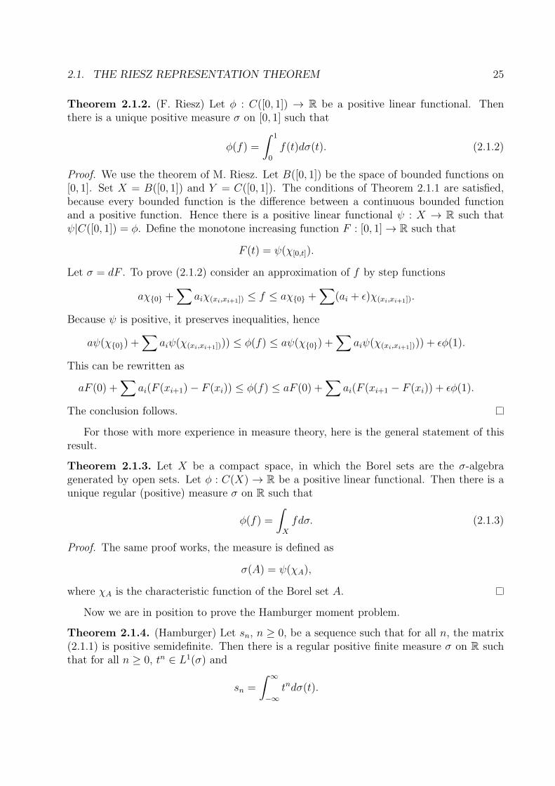
Theorem 2.1.2. (F. Riesz) Let φ : C([0, 1]) → R be a positive linear functional. Thenthere is a unique positive measure σ on [0, 1] such that
φ(f) =
∫ 1
0
f(t)dσ(t). (2.1.2)
Proof. We use the theorem of M. Riesz. Let B([0, 1]) be the space of bounded functions on[0, 1]. Set X = B([0, 1]) and Y = C([0, 1]). The conditions of Theorem 2.1.1 are satisfied,because every bounded function is the difference between a continuous bounded functionand a positive function. Hence there is a positive linear functional ψ : X → R such thatψ|C([0, 1]) = φ. Define the monotone increasing function F : [0, 1] → R such that
F (t) = ψ(χ[0,t]).
Let σ = dF . To prove (2.1.2) consider an approximation of f by step functions
aχ{0} +∑
aiχ(xi,xi+1]) ≤ f ≤ aχ{0} +∑
(ai + ǫ)χ(xi,xi+1]).
Because ψ is positive, it preserves inequalities, hence
aψ(χ{0}) +∑
aiψ(χ(xi,xi+1]))) ≤ φ(f) ≤ aψ(χ{0}) +∑
aiψ(χ(xi,xi+1]))) + ǫφ(1).
This can be rewritten as
aF (0) +∑
ai(F (xi+1)− F (xi)) ≤ φ(f) ≤ aF (0) +∑
ai(F (xi+1 − F (xi)) + ǫφ(1).
The conclusion follows.
For those with more experience in measure theory, here is the general statement of thisresult.
Theorem 2.1.3. Let X be a compact space, in which the Borel sets are the σ-algebragenerated by open sets. Let φ : C(X) → R be a positive linear functional. Then there is aunique regular (positive) measure σ on R such that
φ(f) =
∫
X
fdσ. (2.1.3)
Proof. The same proof works, the measure is defined as
σ(A) = ψ(χA),
where χA is the characteristic function of the Borel set A.
Now we are in position to prove the Hamburger moment problem.
Theorem 2.1.4. (Hamburger) Let sn, n ≥ 0, be a sequence such that for all n, the matrix(2.1.1) is positive semidefinite. Then there is a regular positive finite measure σ on R suchthat for all n ≥ 0, tn ∈ L1(σ) and
sn =
∫ ∞
−∞
tndσ(t).

26 CHAPTER 2. LINEAR FUNCTIONALS
Proof. Denote by R[x] the real valued polynomial functions on R and by Cc(R) the contin-uous functions with compact support. Consider
X = R[x] + Cc(R), Y = R[x],
and
C = {f ∈ X | f(t) ≥ 0 for all t}.
For a polynomial u(t) =∑N
n=0 antn, let
φ0(u) =N∑
n=0
ansn.
Let us show that φ0 is positive on C. We have u ≥ 0 if and only if u = p2 + q2. If p and q
are the vectors with coordinates the coefficients of p and q, then
φ0(u) = φ0(p2) + φ0(q
2) = pTSNp+ qTSNq ≥ 0.
The conditions of Theorem 2.1.1 are verified. Then there is a linear positive functionalφ : X → R such that φ|Y = φ0. By Theorem 2.1.2, on every interval [−m,m], m ≥ 1there is a measure σm such that if f is continuous with the support in [−m,m], then φ(f) =∫ m
−mf(t)dσm(t). Uniqueness implies that for m1 > m2, σm1
|[−m2,m2] = σm2. Hence we can
define σ on R such that σ|[−m,m] = σm. Then for all f ∈ Cc(R),
φ(f) =
∫ ∞
−∞
f(t)dσ(t).
The fact that σ is a finite measure is proved as follows. Given an interval [−m,m], let fbe compactly supported, such that
χ[−m,m] ≤ f ≤ 1.
Then
σ([−m,m]) = φ(χ[−m,m]) ≤ φ(f) ≤ φ0(1) = s0.
Hence σ is finite.Let us now show that
φ(p) =
∫ ∞
−∞
p(t)dσ(t).
If p is an even degree polynomial with positive dominant coefficient, then it can be approxi-mated from below by compactly supported continuous functions, and so using the positivityof φ we conclude that for every such function f
φ(p) ≥ φ(f) =
∫ ∞
−∞
f(t)dσ(t).

2.2. THE RIESZ REPRESENTATION THEOREM FOR HILBERT SPACES 27
By passing to the limit we find that
φ(p) ≥∫ ∞
−∞
p(t)dσ(t).
Let q be a polynomial of even degree with dominant coefficient positive, whose degree is lessthan the degree of p. Then for every a > 0,
φ(p− aq) ≥∫ ∞
−∞
(p− aq)(t)dσ(t).
Said differently
φ(p)−∫ ∞
−∞
p(t)dσ(t) ≥ a
(
φ(q)−∫ ∞
−∞
q(t)dσ(t)
)
.
This can only happen if
φ(q) =
∫ ∞
−∞
q(t)dσ(t).
Varying p and q we conclude that this is true for every q with even degree and with positivedominant coefficient. Since every polynomial can be written as the difference between twoeven degree polynomials with positive dominant coefficients, the property is true for allpolynomials.
2.2 The Riesz Representation Theorem for Hilbert spaces
Theorem 2.2.1. (The Riesz Representation Theorem) Let H be a Hilbert space and letφ : H → C be a continuous linear functional. Then there is z ∈ H such that
φ(x) = 〈x, z〉 , for all x ∈ H.
Proof. Let us assume that φ is not identically equal to zero, for otherwise we can choosez = 0.
Because φ is continuous, Kerφ = φ−1(0) is closed. Let Y = Kerφ⊥. Then Y is onedimensional, because if y1, y2 were linearly independent in Y , then φ(φ(y2)y1−φ(y1)y2) = 0,but φ(y2)y1 − φ(y1)y2 is a nonzero vector orthogonal to the kernel of φ.
Next, let y be a nonzero vector in Y , so that φ(y) 6= 0. Replace y by y′ = y/φ(y). Letz = y′/‖y′‖2. Then
φ(z) = 1/‖y′‖2 = 〈z, z〉 .
Every vector x ∈ H can be written uniquely as x = u + αz with u ∈ Kerφ and α a scalar.Then
φ(x) = φ(u+ αz) = αφ(z) = α 〈z, z〉= 〈u+ αz, z〉 = 〈x, z〉 .

28 CHAPTER 2. LINEAR FUNCTIONALS
Example. If φ : L2(R) 7→ C is a continuous linear functional, then there is an L2 functiong such that
φ(f) =
∫ ∞
−∞
f(t)g(t)dt,
for all f ∈ L2(R).
Example. Consider the Hardy space H2(D), and the linear functionals φz(f) = f(z), z ∈ D.Then for all z, φz is continuous, and so there is a function Kz(w) ∈ H2(D) such that
f(z) = 〈f,Kz〉 .
The function (z, w) 7→ Kz(w) is called the reproducting kernel of the Hardy space.
Example. Consider the Segal-Bargmann space HL2(C, µ~). The linear functionals φz(f) =f(z), z ∈ C are continuous. So we can find Kz(w) ∈ HL2(C, µ~) so that
f(z) =
∫
C
f(w)Kz(w)dµ~.
Again, (z, w) 7→ Kz(w) is called the reproducing kernel of the Segal-Bargmann space.
Remark 2.2.1. Using the Cauchy-Schwarz inequality, we see that
|φ(x)| ≤ ‖z‖‖x‖.
In fact it can be seen that the continuity of φ is equivalent to the existence of an inequalityof the form |φ(x)| ≤ C‖x‖ that holds for all x, where C is a fixed positive constant.
2.3 The Hahn-Banach Theorems
Theorem 2.3.1. (Hahn-Banach) Let X be a real vector space and let p : X → R be afunctional satisfying
p(x+ y) ≤ p(x) + p(y), p(tx) = tp(x)
if x, y ∈ X, t ≥ 0. Also, let Y be a subspace and let φ0 : Y → R be a linear functionalsuch that φ0(y) ≤ p(y) for all y ∈ Y . Then there is a linear functional φ : X → R such thatφ|Y = φ0 and φ(x) ≤ p(x) for all x ∈ X.
Remark 2.3.1. The functional p can be a seminorm, or more generally, a Minkowski func-tional.
Proof. First choose x1 ∈ X such that x1 6∈ Y and consider the space
Y1 = {y + tx1 | y ∈ Y, t ∈ R}.

2.3. THE HAHN-BANACH THEOREMS 29
Because
φ0(y) + φ0(y′) = φ0(y + y′) ≤ p(y + y′) ≤ p(y − x1) + p(x1 + y′)
we have
φ0(y)− p(y − x1) ≤ p(y′ + x1)− φ0(y′)
for all y, y′ ∈ Y . Then there is α ∈ R such that
φ0(y)− p(y − x1) ≤ α ≤ p(y′ + x1)− φ0(y′)
for all y, y′ ∈ Y . Then for all y ∈ Y ,
φ0(y)− α ≤ p(y − x1) and φ0(y) + α ≤ p(y + x1).
Define φ1 : Y1 → R, by
φ1(y + tx1) = φ0(y) + tα.
Then φ1 is linear and coincides with φ on Y . Also, when φ1(y + tα) ≥ 0,
φ1(y + tx1) = |t|φ1(y/|t| ± x1) = |t| (φ0(y/|t|)± α)
≤ |t|p(y/|t| ± x1) = p(y + tx1).
(The inequality obviously holds when φ1(y + tx1) < 0.)To finish the proof, apply Zorn’s lemma to the set of functionals φ : Z → R, with
Y ⊂ Z ⊂ X and φ|Y = φ0, φ(x) ≤ p(x), ordered by φ < φ′ if the domain Z of φ is asubspace of the domain of Z ′ of φ′ and φ′|Z = φ.
Theorem 2.3.2. (Hahn-Banach) Suppose Y is a subspace of the vector space X, p is aseminorm on X, and φ0 is a linear functional on Y such that |φ0(y)| ≤ p(y) for all y ∈ Y .Then there is a linear functional φ on X that extends φ0 such that |φ(x)| ≤ p(x) for allx ∈ X.
Proof. This is an easy consequence of the previous result. If we work with real vector spaces,then because φ is linear, by changing x to −x if necessary, we get |φ(x)| ≤ p(x) for all x.
If X is a complex vector space, note that a linear functional can be decomposed asφ = Reφ+ iImφ. Then Reφ(ix) = −Imφ(x), so φ(x) = Reφ(x) + iReφ(ix). So the real partdetermines the functional.
Apply the theorem to Reφ0 to obtain Reφ, and from it recover φ. Note that for everyx ∈ X, there is α ∈ C, |α| = 1 such that αφ(x) = |φ(x)|. Then
|φ(x)| = |φ(αx)| = φ(αx) = Reφ(αx) ≤ p(αx) = p(x).
The theorem is proved.
Definition. Let X be a vector space, A,A′ ⊂ X, φ : X → R. We say that a nontrivialfunctional φ separates A from A′ if φ(x) ≤ φ(x′) for all x ∈ A and x′ ∈ A′.

30 CHAPTER 2. LINEAR FUNCTIONALS
Definition. Let B be a convex set, x0 ∈ B. We say that x0 is internal to B if B − x0 ={b− x0 | b ∈ B} is absorbing.
Theorem 2.3.3. (Hahn-Banach) Let X be a vector space, A,A′ convex subsets of X, A ∩A′ = ∅ and A has an internal point. Then A and A′ can be separated by a nontrivial linearfunctional.
Proof. Fix a ∈ A, a′ ∈ A′ such that a is internal to A. Consider the set
B = {x− x′ − a+ a′ | x ∈ A, x′ ∈ A′}.
It is not hard to check that B is convex, it is also absorbing. Consider the Minkowskifunctional µB. Because A and A′ are disjoint, a′ − a 6∈ B. Hence µB(a
′ − a) ≥ 1.Set Y = R(a′ − a) and define φ0(λ(a
′ − a)) = λ. Then φ0(y) ≤ µB(y) for all y ∈ Y . Bythe first Hahn-Banach theorem, there is φ : X → R such that φ(x) ≤ µB(x) for all x ∈ X,and also φ(a′ − a) = φ0(a
′ − a) = 1.If x ∈ B, then µB(x) ≤ 1, so φ(x) ≤ 1. Hence if x ∈ A, x′ ∈ A′, then
φ(x− x′ − a+ a′) ≤ 1.
In other words
φ(x− x′) + φ(a′ − a) ≤ 1, for all x ∈ A, x′ ∈ A′.
Since φ(a′ − a) = 1, it follows that φ(x− x′) ≤ 0, so φ(x) ≤ φ(x′) for all x ∈ A, x′ ∈ A′.
Theorem 2.3.4. (Hahn-Banach) Suppose A and B are disjoint, nonempty, convex sets ina locally convex topological vector space X.a) If A is open then there is a continuous linear functional φ on X and γ ∈ R such that
Reφ(x) < γ ≤ Reφ(y) for all x ∈ A, y ∈ Y.
b) If A is compact and B is closed then there is a continuous linear functional φ and γ1, γ2 ∈ R
such that
Reφ(x) ≤ γ1 < γ2 ≤ Reφ(y)
for all x ∈ A and y ∈ B.
Proof. We consider only the real case. Because A is open, every point of A is internal. Sothere is φ and α such that A ⊂ {x |φ(x) ≤ α} and B ⊂ {x |φ(x) ≥ α}. Let x0 be a pointin A. Then for every x ∈ A, φ(x − x0) = φ(x) − φ(x0) ≤ α − φ(x0). So there is an openneighborhood A− x0 of 0 such that φ(y) ≤ β if y ∈ A− x0, where β = α− φ(x0). ChoosingV ⊂ A− x0 to be a balanced neighborhood of 0, we conclude that |φ(y)| ≤ β for all y ∈ V .But this is the condition that φ is continuous.
We claim that because A is open φ(x) < α for all x ∈ A. If not, let x be such thatφ(x) = α. Consider a neighborhood V ⊂ of x such that V − x is a balanced convexneighborhood of 0. Then for every y ∈ V there is z ∈ V such that x is the midpoint ofthe segment yz. We have φ(x) = 1
2φ(y) + 1
2φ(z), and because φ(y) and φ(z) are both less

2.4. A FEW RESULTS ABOUT CONVEX SETS 31
than or equal to α, φ(y) = φ(z) = φ(x) = α. Hence φ is constant in a neighborhood of x.Consequently φ is constant in a neighborhood of 0, and because the neighborhoods of 0 areabsorbing, it is constant everywhere. This is impossible. Hence a) is true.
For b) we use Proposition 1.3.3 to conclude that there is an open set U such that (A +U) ∩ (B + U) = ∅. By shrinking, we can make U balanced and convex. Then A + U andB+U are openand convex. Now use part a) to construct a continuous linear functional thatseparates A+ U from B + U . Let x0 ∈ U\{0} such that φ(x0) = γ > 0. Then
supx∈A
φ(x) + γ ≤ supx∈A+U
φ(x), infy∈B
φ(y)− γ ≥ infy∈B+U
φ(y).
The conclusion follows.
2.4 A few results about convex sets
For a subset A of a vector spaceX, we denote by Ext(A) the extremal points of A, namely thepoints x ∈ A which cannot be written as x = ty+(1− t)z with y, z ∈ A\{x}, t ∈ (0, 1). Thisdefinition can be extended from points to sets by saying that a subset B of A is extremal iffor x, y ∈ A and t ∈ (0, 1) such that tx+(1− t)y ∈ B, it automatically follows that x, y ∈ B.Note that a point x is extremal if an only if {x} is an extremal set.
Also, for a subset A of the vector space X, we denote by co(A) the convex hull of A,namely the convex set consisting of all points of the form tx + (1− t)y where x, y ∈ A andt ∈ [0, 1].
Theorem 2.4.1. (Krein-Milman) Suppose X is a locally convex topological vector space,and let K be a subset of X that is compact and convex. Then
K = co(Ext(K)).
Proof. Let us define the family of sets
F = {K ′ ⊂ K |K ′ : closed, convex, nonempty, and extremal in K}.
If G is a subfamily that is totally ordered by inclusion, then because K is compact,
K0 = ∩K′∈GK′ 6= ∅.
It is not hard to see that K0 is also extremal. Hence we are in the conditions of Zorn’sLemma. We deduce that F has minimal elements.
Let Km be a minimal element; we claim it is a singleton. Arguing by contradiction,let us assume that Km has two distinct points. By the Hahn-Banach Theorem there is acontinuous linear functional φ : X → R such that φ(x) 6= φ(y). Let
α = maxx∈Km
φ(x).
Define
K1 = {y ∈ K0 |φ(y) = α}.

32 CHAPTER 2. LINEAR FUNCTIONALS
Then K1 is a nonempty extremal subset of Km and consequently an extremal subset of K.It is also compact and convex, which contradicts the minimality of Km. Hence Km containsonly one point. This proves
Ext(K) 6= ∅.
Let Ke = co(Ext(K)). Note that Ke is compact. Assume Ke 6= K. Then there is x ∈ K\Ke.By the Hahn-Banach theorem, there is a continuous linear functional φ : X → R such thatmaxy∈Ke
φ(y) < φ(x). Set
K2 = {z ∈ K |φ(z) = maxy∈K
φ(y)}.
It is not hard to see that K2 is extremal in K. Hence K2 ∈ F . Applying again Zorn’sLemma, we conclude that there is a minimal extremal set in K that is included in K2. Thisminimal set is a singleton. So there is y ∈ K2 ∩ Ext(K). But K2 is disjoint from Ext(K),which is a contradiction. The conclusion follows.
Theorem 2.4.2. (Milman) Let X be a locally convex topological vector space. Let K be acompact set such that co(K) is also compact. Then every extreme point of co(K) lies in K.
Proof. Assume that some extreme point x0 ∈ co(K) is not in K. Then there is a convexbalanced neighborhood V of 0 in X such that
(x0 + V ) ∩K = ∅.
Choose x1, x2, . . . , xn ∈ K such that K ⊂ ∪nj=1(xj + V ). Each of the sets
Kj = co(K ∩ (xj + V )), 1 ≤ j ≤ n
is compact and convex. Note in particular that, because V is convex,
Kj ⊂ xj + V = xj + V .
Also K ⊂ K1 ∪ · · · ∪ Kn. We claim that co(K1 ∪ K2 ∪ · · · ∪ Kn) is compact as well.To prove this, let σ = {(t1, t2, . . . , tn) ∈ [0, 1]n | ∑j tj = 1}, and consider the functionf : σ ×K1 ×K2 . . .×Kn → X,
f(t1, . . . , tn, k1, . . . , kn) =∑
j
tjkj .
Let C be the image of f . Note that C ⊂ co(K1 ∪K2 · · · ∪Kn). Clearly C is compact, beingthe image of a compact set, and is also convex. It contains each Kj, and hence it coincideswith co(K1 ∪K2 · · · ∪Kn).
So
co(K) ⊂ co(K1 ∪ · · · ∪Kn).
The opposite inclusion also holds, because Kj ⊂ co(K) for every j. Hence
co(K) = co(K1 ∪ · · · ∪Kn).

2.4. A FEW RESULTS ABOUT CONVEX SETS 33
In particular,
x0 = t1y1 + t2y2 + · · ·+ tnyn,
where yj ∈ Kj and tj ≥ 0,∑
tj = 1. But x0 is extremal in co(K), so x0 coincides with oneof the yj. Thus for some j,
x0 ∈ Kj ⊂ xj + V ⊂ K + V ,
which contradicts our initial assumption. The conclusion follows.
We will show an application of these results. Given a convex subset K of a vector spaceX, and a vector space Y , a map T : K → Y is called affine if for every x, y ∈ K and t ∈ [0, 1],
T (tx+ (1− t)y) = tT (x) + (1− t)T (y).
The result is about groups of affine transformations from X into itself. If X has a topologicalvector space structure, a group G of affine transformations ofK is called equicontinuous if forevery neighborhood V of 0 in X, there is a neighborhood U of 0 such that T (x)− T (y) ∈ Vfor every x, y ∈ K such that x− y ∈ U and for every T ∈ G.
Theorem 2.4.3. (Kakutani’s Fixed Point Theorem) Suppose thatK is a nonempty compactconvex subset of a locally convex topological vector space X and that G is an equicontinuousgroup of affine transformations taking K into itself. Then there is x0 ∈ K such that T (x0) =x0 for all T ∈ G.
Proof. Let
F = {K ′ ⊂ K |K ′ : nonempty, compact, convex , T (K ′) ⊂ K ′ for all T ∈ G}.
Note that K ∈ F , so this family is nonempty. Order F by inclusion and note that if G is asubfamily that is totally ordered, then because K is compact,
K0 = ∩K′∈GK′ 6= ∅.
Clearly T (K0) ⊂ K0, so the conditions of Zorn’s lemma are satisfied. It follows that F hasminimal elements. Let K0 be such a minimal element. We claim that it is a singleton.
Assume, to the contrary, that K0 contains x, y with x 6= y. Let V be a neighborhood of0 such that x− y 6∈ V , and let U be the neighborhood of 0 associated to U by the definitionof equicontinuity. Then for every T ∈ G, T (x)− T (y) 6∈ U , for else, because T−1 ∈ G,
x− y = T−1(T (x))− T−1(T (y)) ∈ V.
Set z = 12(x+ y). Then z ∈ K0. Let
G(z) = {T (z) |T ∈ G}.
Then G(z) is G-invariant, hence so is its closure K1 = G(z). Consequently, co(K1) is aG-invariant, compact convex subset of K0. The minimality of K0 implies
K0 = co(K1).

34 CHAPTER 2. LINEAR FUNCTIONALS
By the Krein-Milman Theorem (Theorem 2.4.1), K0 has extremal points. Applying Milman’sTheorem (Theorem 2.4.2), we deduce that every extremal point of K0 lies in K1. Let x0 bean extremal point.
Consider the set
S = {(Tz, Tx, Ty) |T ∈ G} ⊂ K0 ×K0 ×K0.
Since x0 ∈ K1 = G(z), and K0 × K0 is compact, there is a point (x1, y1) ∈ K0 × K0 suchthat (x0, x1, y1) ∈ S. Indeed, if this were not true, then every (x1, y1) ∈ K0×K0 would havea neighborhood W(x1,y1) for which there would exist a neighborhood V(x1,y1) of x0 such thatV(x1,y1) ×W(x1,y1) ∩ S = ∅. Then K0 ×K0 is covered by finitely many of the W(x1,y1) and theintersection of the corresponding V(x1,y1)’s is a neighborhood of p that does not intersect K1.
Because 2Tz = Ty + Ty for all T , we get 2x0 = x1 + y1, hence x0 = x1 = y1, because x0is an extremal point. But Tx − Ty 6∈ V for all T ∈ G, hence x1 − y1 6∈ V , and so x1 6= y1.This is a contradiction, which proves our initial assumption was false, and the conclusionfollows.
2.5 The dual of a topological vector space
2.5.1 The weak∗-topology
Let X be a topological vector space.
Definition. The space X∗ of continuous linear functionals on X is called the dual of X.
X∗ is a vector space. We endow it with the weak∗ topology, in which a system ofneighborhoods of the origin is given by
V (x1, x2, . . . , xn, ǫ) = {φ ∈ X∗ | |φ(xj)| < ǫ, j = 1, 2, . . . , n},
where x1, x2, . . . , xn range in X and ǫ > 0.
Proposition 2.5.1. The space X∗ endowed with the weak∗ topology is a locally convextopological vector space.
The Hahn-Banach Theorem implies automatically that the weak∗-continuous linear func-tionals on X∗ separate the points of this space. Each point x ∈ X defines a weak∗-continuouslinear functional x∗ on X∗ defined by
x∗(φ) = φ(x).
In fact we have the following result.
Theorem 2.5.1. Every weak∗-continuous linear functional on X∗ is of the form x∗ for somex ∈ X. Hence (X∗)∗ = X. 1
1It is important that on X∗ we have the weak∗ topology, if we put a different topology on it, (X∗)∗ might
not equal X.

2.5. THE DUAL OF A TOPOLOGICAL VECTOR SPACE 35
Proof. Assume that φ∗ is a weak∗-continuous linear functional on X∗. Then |φ∗(φ)| < 1for all φ in some set V (x1, x2, . . . , xn, ǫ). This means that there is a constant C such that|φ∗(φ)| ≤ Cmaxj |x∗j(φ)| for all φ ∈ X∗.
Let N be the set on which x∗j = 0, j = 1, 2, . . . , n. Then φ∗ is zero on N , so we canfactor X∗ by N so that we are in the finite dimensional situation. We can identify X∗/Nwith Span(x1, x2, . . . , xn)
∗. In X∗/N , φ∗ =∑
j αjx∗j , and so this must be the case in X as
well. Hence
φ∗ = (∑
j
αjxj)∗,
and we are done.
Theorem 2.5.2. (Banach-Alaoglu) Let X be a topological vector space, V a neighborhoodof 0 and
K = {φ ∈ X∗ | |φ(x)| ≤ 1, for all x ∈ V }.
Then K is compact in the weak∗ topology.
Proof. Let x ∈ V , and define
Kx = {λ ∈ C | |λ| ≤ 1}.
The set∏
x∈V
Kx
is compact in the product topology, by Tychonoff’s Theorem. Define
Φ : K →∏
x∈V
Kx, Φ(φ) = (φ(x))x∈V .
We will show
(1) Φ(K) is closed.
(2) Φ : K → Φ(K) is a homeomorphism.
For (1) assume that (ax)x∈V is in Φ(K). Define φ(x) = 1tatx for t such that tx ∈ V ,
Approximating (ax)x∈V with linear functionals φn ∈ Φ(K), n = 1, 2, . . . , n. we have
φn(αx+ βy) = αφn(x) + βφn(y).
For n large enough, φn(αx+βy) approximates well φ(x), while φn(x) and φn(y) approximateφ(x) and φ(y). By passing to the limit n→ ∞ we obtain that φ is linear.
Also for x ∈ V , |φn(x)| ≤ 1, and again by passing to the limit, |φ(x)| ≤ 1. This impliesthe continuity of φ, as well as the fact that it lies in Φ(K). This proves (1).
For (2), note that Φ is one-to-one, hence it is an inclusion. Moreover, the weak∗ topologywas chosen so that it coincides with the topology induced by the product topology. Hence(2).

36 CHAPTER 2. LINEAR FUNCTIONALS
2.5.2 The dual of a normed vector space
If X is a normed vector space, then X∗ is also a normed space with the norm
‖φ‖ = sup{φ(x) | ‖x‖ ≤ 1}.
Proposition 2.5.2. The dual of a normed space is a Banach space.
Proof. The only difficult part is to show that X∗ is complete. Let φn, n ≥ 1, be a Cauchysequence in X∗. Define φ(x) = limn→∞ φn(x). It is not hard to check that φ is linear. Onthe other hand, because φn is Cauchy, ‖φn‖ is Cauchy as well, by the triangle inequality(|‖φn‖ − ‖φm‖| < ‖φn − φm‖). For a given x, if we choose n large enough then
|φ(x)− φn(x)| < ‖x‖,
so
|φ(x)| < (‖φn‖+ 1)‖x‖.
Because ‖φn‖, n ≥ 1 is a bounded sequence (being Cauchy), it follows that φ is a boundedlinear functional, and we are done.
So X∗ has two topologies the one induced by the norm, and the weak∗ topology. It isnot hard to check that the second is weaker than the first. Here is an example of the dualof a Banach space.
Theorem 2.5.3. Let p ∈ [1,∞). Then (Lp([0, 1]))∗ = Lq([0, 1]), where q satisfies
1
p+
1
q= 1.
A function g ∈ Lq([0, 1]) defines a functional by
φg(f) =
∫ 1
0
f(x)g(x)dx.
Proof. Note that every g ∈ Lq([0, 1]) defines a continuous linear functional by the aboveformula because of Holder’s inequality:
‖fg‖1 ≤ ‖f‖p‖g‖q.
Moreover, it is not hard to see that if g1 and g2 define the same functional then g1 = g2almost everywhere. This follows from the fact that if
∫ 1
0
f(x)[g1(x)− g2(x)]dx = 0
for all f then g1 − g2 = 0 almost everywhere.Let us show that every continuous linear functional φ is of this form. The map
µφ : A 7→ φ(χA)

2.5. THE DUAL OF A TOPOLOGICAL VECTOR SPACE 37
is a measure on the Lebesgue measurable sets in [0, 1]. Note that µφ is absolutely continuouswith respect to the Lebesgue measure, since if the Lebesgue measure of A is zero, then χA
is the zero vector in Lp([0, 1]), and so µφ(A) = φ(χA) = 0.Using the Radon-Nikodym Theorem, we deduce that there is a function g ∈ L1([0, 1])
such that
φ(χA) =
∫ 1
0
χA(x)g(x)dx. (2.5.1)
Case 1. p = 1. We have∣
∣
∣
∣
∫
A
g(x)dx
∣
∣
∣
∣
= |φ(χA)| ≤ ‖φ‖‖χA‖1 = ‖φ‖m(A),
where m(A) is the Lebesgue measure of A. So |g| ≤ ‖φ‖ almost everywhere, showing thatg ∈ L∞([0, 1]).Case 2. p > 1. Looking at (2.5.1) and approximating the functions in Lp([0, 1]) by stepfunctions, and using the continuity of both the left-hand side on Lp([0, 1]) and of the right-hand side on L∞([0, 1]) ⊂ Lp([0, 1]), we deduce that
φ(f) =
∫ 1
0
f(x)g(x)dx for all f ∈ Lp([0, 1]).
We want to show that if∫ 1
0f(x)g(x)dx is finite for all f ∈ Lp([0, 1]), then g ∈ Lq([0, 1]). By
multiplying f by |g|/g, we can make g be positive, so let us consider just this case.Let h be a step function that approximates gq from below, h ≥ 0. Consider
φ(h1/p) =
∫ 1
0
g(x)h1/p(x)dx ≥∫ 1
0
h1/q(x)h1/p(x)dx =
∫ 1
0
h(x)dx.
By the continuity of φ, this inequality forces∫ 1
0
h(x)dx ≤ ‖φ‖‖h1/p‖p. (2.5.2)
We also have
‖h1/p‖p =[∫ 1
0
h(x)dx
]1/p
,
so from (2.5.2) we get
∫ 1
0
h(x)dx ≤ ‖φ‖(∫ 1
0
h(x)dx
)1/p
.
Dividing through we get
(∫ 1
0
h(x)dx
)1/q
≤ ‖φ‖.
Passing to the limit with h→ gq, we obtain ‖g‖q ≤ ‖φ‖, as desired.

38 CHAPTER 2. LINEAR FUNCTIONALS
Here is this result in full generality.
Theorem 2.5.4. Let (X,µ) be a measure space, and let p ∈ [1,∞) and q such that 1/p +1/q = 1. Then (Lp(X))∗ = Lq(X), where g ∈ Lq(X) defines the functional
φ(f) =
∫
X
fgdµ.
Moreover ‖φ‖ = ‖g‖q.Theorem 2.5.5. (C([0, 1]))∗ is the set of finite complex valued measures on [0, 1].
Proof. Each finite measure µ defines a continuous linear functional by
φ(f) =
∫ 1
0
f(t)dµ.
Let us prove conversely, that every linear functional is of this form. For every complexcontinuous linear functional φ, we have φ = Reφ + iImφ where the real and the imaginarypart are themselves continuous. So we reduce the problem to real functionals. We show thateach such functional is the difference between two positive functionals, and then apply theRiesz Representation Theorem.
For f ≥ 0, set
φ+(f) = sup{φ(g) | g ∈ C([0, 1]), 0 ≤ g ≤ f}.Because φ is continuous, hence bounded, φ+ takes finite values. Since g = 0 ≤ f , andφ(0) = 0, we have that φ+ is positive.
It is clear that φ+(cf) = cφ+(f), for c ≥ 0, f ≥ 0.Also, for f1, f2 ≥ 0, φ+(f1 + f2) ≥ φ+(f1) + φ+(f2) because we can use for f1 + f2 the
function g1 + g2 with 0 ≤ g1 ≤ f1 and 0 ≤ g2 ≤ f2. On the other hand, if f = f1 + f2, andg ≤ f , set g1 = max(g − f2, 0) and g2 = min(g, f2). Then g1 + g2 = g, and 0 ≤ gj ≤ fj,j = 1, 2. Hence
φ(g) = φ(g1) + φ(g2) ≤ φ+(f1) + φ+(f2).
Consequently φ+(f) = φ+(f1 + f2) ≤ φ+(f1) + φ+(f2). Therefore we must have equality.For arbitrary f , write f = f1− f2, where f1, f2 ≥ 0, and define φ+(f) = φ+(f1)−φ+(f2).
It is not hard to see that φ+ is well defined, linear, and positive. Also φ+ − φ is a linearpositive functional. We have
φ = φ+ − (φ+ − φ),
and the claim is proved. We can therefore write every continuous complex linear functionalas
φ = φ1 − φ2 + i(φ3 − φ4),
where φj, j = 1, 2, 3, 4 are positive. Each of these is given by a positive measure µj, by theRiesz representation Theorem, so φ is given by the complex measure
µ = µ1 − µ2 + i(µ3 − µ4).

2.5. THE DUAL OF A TOPOLOGICAL VECTOR SPACE 39
Remark 2.5.1. Using the general form of the Riesz Representation Theorem, we see that[0, 1] can be replaced by any compact space.
Theorem 2.5.6. (Banach-Alaoglu) Let X be a normed vector space. Then the closed unitball in X∗ is weak∗-compact.
Here are some applications.
Proposition 2.5.3. Place a number from the interval [0, 1] at each node of the lattice Z2
such that the number at each node is the average of the four numbers at the closest nodes.Then all numbers are equal.
Proof. Consider the Banach space L∞(Z2). LetK be the set of elements in L∞(Z2) satisfyingthe condition from the statement. Then K is a weak∗-closed subset of the unit ball; byapplying the Banach-Alaoglu theorem we deduce that it is weak∗-compact. It is also convex.By the Krein-Milman Theorem, K = co(Ext(K)). Let f : Z2 → [0, 1] be an extremal point inK. Let L, U be the operators that shift up and left. Then Uf, U−1f, Lf, L−1f are functionswith the same property, and
f =1
4(Uf + U−1f + Lf + L−1f).
Because f is extremal, f = Uf = U−1f = Lf = L−1f , meaning that f is constant. Infact f = 0 or f = 1. The convex hull of the two extremal constant functions is the set ofall constant functions with values in [0, 1], this set is closed, so K consists only of constantfunctions. Done.
Theorem 2.5.7. The space L1(R) is not the dual of any normed space.
Proof. If L1(R) were the dual of a normed space, then the Banach-Alaoglu Theorem impliesthat the closed unit ball in L1(R) is weak∗-compact. By the Krein-Milman Theorem it hasextreme points. But this is not true, since every function in the closed unit ball of L1 canbe written as the convex combination of two functions in the unit ball.
Remark 2.5.2. Here we should compare with the case of Lp spaces. Just focus on positivefunctions. The convex combination of two norm 1 such functions in L1 has also norm 1. Butthis is not true for Lp spaces.
Consider C([0, 1]), the Banach space of continuous functions on [0, 1], with the norm‖f‖ = supx∈[0,1] |f(x)|.
Theorem 2.5.8. (Stone-Weierstrass) Let A ⊂ C([0, 1]) be a subalgebra with the followingproperties
(1) if f ∈ A then f ∈ A,
(2) the function identically equal to 1 is in A,
(3) A separates the points of [0, 1].
Then A is dense in C([0, 1]).

40 CHAPTER 2. LINEAR FUNCTIONALS
Proof. (de Brange) We argue by contradiction. Let
K = {φ ∈ C([0, 1])∗ | ‖φ‖ ≤ 1, φ|A = 0}.
By the Banach-Alaoglu Theorem, it is compact in the weak∗ topology. K is also convex, soby the Krein-Milman Theorem it has extremal points. Moreover, the Hahn-Banach Theoremimplies that K 6= {0}, so then Krein-Milman implies the existence of at least two extremalpoints. This means that there is an extremal functional φ ∈ K that is not identically equalto zero.
Because C([0, 1])∗ is the space of finite complex measures (Theorem 2.5.5), φ is given bya measure µ. We claim that every function in A is constant on the support of µ. If this is sothen because the functions in A separate points, the support of µ consists of just one point,so µ = cδx0
for x0 ∈ [0, 1] and c ∈ C. Because µ|A = 0, and 1 ∈ A, we get that c = 0, acontradiction. Hence the conclusion.
Let us prove the claim. Suppose there is f ∈ A not constant on the support of µ. Wehave f = f1 + if2, so f1 = (f + f)/2 and f2 = (f − f)/2i, and because f ∈ A, f1, f2 ∈ A aswell. One of these is nonconstant, so we may assume that f is real valued. Replacing f by(f + A)/B we may assume 0 ≤ f ≤ 1. Define the measures µ1 and µ2 by
dµ1 = fdµ, dµ2 = (1− f)dµ.
Then µ = µ1 + µ2. Note that µ1, µ2 are both zero on A.We have ‖µ1‖ =
∫ 1
0fd|µ|, ‖µ2‖ =
∫ 1
0(1− f)d|µ|. And also ‖µ‖ =
∫
d|µ| = ‖µ1‖ + ‖µ2‖.Then
µ =‖µ1‖‖µ‖
( ‖µ‖‖µ1‖
µ1
)
+‖µ2‖‖µ‖
( ‖µ‖‖µ2‖
µ2
)
.
Note that
‖µ‖‖µ1‖
µ1,‖µ‖‖µ2‖
µ2 ∈ K
Because µ is an extreme point, either µ1 or µ2 is zero. So f must be identically equal to 1,a contradiction. The claim is proved, and so it the theorem.
Remark 2.5.3. Using the general form of the Riesz Representation Theorem, we see that[0, 1] can be replaced by any compact space.

Chapter 3
Fundamental Results about Bounded
Linear Operators
3.1 Continuous linear operators
3.1.1 The case of general topological vector spaces
We now start looking at continuous linear operators between topological vector spaces:
T : X → Y.
Proposition 3.1.1. Let T : X → Y be a linear operator between topological vector spacesthat is continuous at 0. Then T is continuous everywhere, moreover, for every open neighbor-hood V of 0 there is an open neighborhood U of 0 such that if x− y ∈ U then Tx−Ty ∈ V .
Definition. A linear operator is called bounded if it maps bounded sets to bounded sets.
Proposition 3.1.2. A continuous linear operator is bounded.
Proof. Let T : X → Y be a continuous linear operator. Consider a bounded set E ⊂ X. Letalso V be a neighborhood of 0 in Y . Because T is continous, there is a neighborhood U of 0 inX such that T (U) ⊂ V . Choose λ ∈ C\{0} such that λE ⊂ U . Then T (λE) = λT (E) ⊂ V .It follows that T (E) is bounded.
Definition. Let T : X → Y be a linear operator. The kernel of T is
ker(T ) = {x ∈ X |Tx = 0}.
The range or image of T is
im(T ) = {y ∈ Y | there is x ∈ X with Tx = y}.
Both ker(T ) and im(T ) are vector spaces. If T is a continuous linear operator betweentopological vector spaces, then ker(T ) is closed. This is not necessarily true about im(T ).
41

42CHAPTER 3. FUNDAMENTAL RESULTS ABOUT BOUNDED LINEAROPERATORS
3.2 The three fundamental theorems
3.2.1 Baire category
Definition. A topological space is said to be of the first category if it is a countable unionof nowhere dense subsets. Otherwise it is said to be of the second category.
Theorem 3.2.1. (Baire Category Theorem) A complete metric space is of the second cat-egory.
Proof. Assume by contradiction that X is a complete metric space of the first category.Write X = ∪∞
n=1Xn, with Xn = X\Vn where Vn is a dense open set. Define inductively theset of balls Bn such that Bn ⊂ Vn and Bn ⊂ Bn−1. The centers of the balls form a Cauchysequence that converges to a point x ∈ X. This point x belongs to all Bn and hence it is inthe complement of every Xn. But this is impossible because X is the union of all Xn.
Corollary 3.2.1. If X is of second category and X = ∪∞n=1Xn, then there is n such that Xn
contains an open subset.
3.2.2 Bounded linear operators on Banach spaces
From now on we will focus just on continuous linear operators between Banach spaces.
Theorem 3.2.2. Let T : X → Y be a linear operator. Then T is continuous if and only ifit is bounded.
Proof. We have seen that if T is continuous then T is bounded. Let us show the converse.Assume that T is bounded by is not continuous. Then there is a neighborhood V ⊂ Yof 0 such that T−1(V ) is not a neighborhood of 0. This means that there is a sequencexn ∈ X\T−1(V ) such that xn → 0. So there is a sequence xn → 0 such that Txn 6∈ V , n ≥ 1.We know that T is bounded, so {Txn}n is bounded. But now we can write xn = αnyn, whereαn → 0 and yn → 0. Then {Tyn}n is still bounded, which implies that Txn = αnTyn → 0.This is a contradiction. Hence T is bounded.
Definition. Let T be a bounded linear operator (which is the same as a continuous operator).The norm of T is
‖T‖ = sup{‖Tx‖ | ‖x‖ ≤ 1}.Here is one example from P.D. Lax, Functional Analysis:
Example. An example of a bounded linear operator is the Laplace transform:
L : L2([0,∞)) → L2([0,∞)), (Lf)(s) =
∫ ∞
0
f(t)e−stdt.
Let us prove that it is indeed a bounded linear operator and let us compute its norm. Wehave
|(Lf)(s)|2 =(∫ ∞
0
f(t)e−stdt
)2
=
(∫ ∞
0
(f(t)e−st/2t1/4)(e−2st/2t−1/4)dt
)2
≤∫ ∞
0
|f(t)|2e−stt1/2dt
∫ ∞
0
e−stt−1/2dt,

3.2. THE THREE FUNDAMENTAL THEOREMS 43
where for the last step we have applied the Cauchy-Schwarz inequality. By changing variableswe can compute the second integral as
∫ ∞
0
e−stt−1/2dt = s−1/2
∫ ∞
0
e−uu−1/2du = s−1/2
∫ ∞
0
e−x2
x−12xdx
= 2s−1/2
∫ ∞
0
e−x2
dx = s−1/2√π.
We conclude that
|(Lf)(s)|2 ≤ s−1/2√π
∫ ∞
0
|f(t)|2e−stt1/2dt.
Integrating with respect to s we obtain
‖Lf‖2 =∫ ∞
0
|(Lf)(s)|2ds ≤ √π
∫ ∞
0
∫ ∞
0
|f(t)|2e−stt1/2s−1/2dtds
=√π
∫ ∞
0
∫ ∞
0
|f(t)|2e−stt1/2s−1/2dsdt =√π
∫ ∞
0
|f(t)|2∫ ∞
0
e−stt1/2s−1/2dsdt
=√π(√π‖f‖2),
where for the last step we have used the integral computed above. Hence ‖Lf‖ ≤ √π‖f‖.
Thus ‖L‖ ≤ √π.
By carefully choosing the function f we can show that ‖L‖ ≥ √π−ǫ for all ǫ (for example
for f = 1/√t on an interval [a, b] with a very small and b very large). Thus ‖L‖ =
√π.
Theorem 3.2.3. (Banach-Steinhaus) Let X be a Banach space, let Y be a normed space,and let F be a family of continuous operators from X to Y . Suppose that for all x ∈ X,supT∈F ‖Tx‖ <∞. Then supT∈F ‖T‖ <∞.
Proof. Let
Xn = {x ∈ X | ‖Tx‖ ≤ n for all T ∈ F}.These sets are convex and balanced. They are also closed, so by the Baire Category Theoremthere is n such that the interior of Xn is nonempty. Because Xn is convex and balanced, itsinterior contains the origin. Hence there is a ball B0,r centered at origin such that ‖Tx‖ ≤ nfor all T ∈ F and x with ‖x‖ ≤ r. We have ‖T‖ ≤ n/r for all T ∈ F , and the theorem isproved.
Here is an application that I have learned from Hari Bercovici. We have
1
x+ 1=
∞∑
n=1
(−1)n−1xn−1.
The left-hand side takes the value 1/2 when x = 1, so it is natural to impose that theright-hand side converges to 1/2. A way to do this is to consider the sequence sn =∑n
k=1(−1)k−1xk−1 and then notice that
1
n(s1 + s2 + · · ·+ sn) (3.2.1)
converges to the same limit as sn when the latter converges (Cesaro), but moreover for x = 1(3.2.1) converges to 1/2.

44CHAPTER 3. FUNDAMENTAL RESULTS ABOUT BOUNDED LINEAROPERATORS
Definition. A summation method associates to each convergent sequence sn, n ≥ 1 anotherconvergent sequence σn, n ≥ 1 such that
(1) limn→∞ σn = limn→∞ sn;
(2) σn =∑∞
k=1 αnksk for n = 1, 2, . . ., where αnk is an array of complex numbers that doesnot depend on sn and defines the summation method.
An example of a summation method, introduced by Cesaro, is αnk = 1/n, n = 1, 2, . . .,1 ≤ k ≤ n, and αnk = 0 otherwise.
Theorem 3.2.4. (Toeplitz) The array αnk, n, k ≥ 1, defines a summation method if andonly if it satisfies the following three conditions
(1) limn→∞ αnk = 0, for all k = 1, 2, . . .;
(2) limn→∞
∑∞k=1 αnk = 1;
(3) supn
∑∞k=1 |αnk| <∞.
Proof. Let us prove that the three conditions are necessary. If sn = δnk for some k, thenσn = αnk. The fact that sn → 0 implies limn→∞ αnk = 0, hence (1).
If sn = 1, n ≥ 1, then σn =∑∞
k=1 αnk. Because sn → 1, it follows that limn→∞
∑
k αnk =1, hence (2).
For (3) we apply the Banach-Steinhaus Theorem. Denote by C0 the Banach space ofconvergent sequences with the sup norm (i.e. continuous functions on N ∪ {∞} with thesup norm, where N ∪ {∞} is given the topology such that the map f(x) = 1/x from it to R
is a homeomorphism onto the image). Let αn, n ≥ 1, be a sequence such that∑∞
n=1 αnxnconverges for every convergent sequence xn, n ≥ 1. We claim that
∑∞n=1 |αn| <∞.
Indeed, if this is not the case, then choose rn > 0 such that that rn → 0 and∑ |αn|rn =
∞. The sequence xn = rnαn/|αn| converges to 0, but∑
n αnxn =∑ |αn|rn = ∞, which is
impossible. This proves our claim.Additionally,
sup(xn)n∈C0,‖(xn)n‖≤1
∣
∣
∣
∣
∣
∑
n
αnxn
∣
∣
∣
∣
∣
=∞∑
n=1
|αn|.
The fact that the left-hand side does not exceed the right-hand side follows from the triangleinequality. On the other hand, if xn = αn/|αn| for 1 ≤ n ≤ N and zero otherwise makes∑
αnxn =∑N
n=1 |αn|. Taking N → ∞ we obtain that the right-hand side is less than orequal to the left-hand side. Hence the two are equal.
Define
φn : C0 → C, φn((sk)k) =∞∑
k=1
αnksk.
Then φn ∈ (C0)∗ and
‖φn‖ =∞∑
k=1
|αnk|.

3.2. THE THREE FUNDAMENTAL THEOREMS 45
The sequence φn((sk)k), n ≥ 1 is bounded for all convergent sequences (sk)k. Hence by theBanach-Steinhaus Theorem, ‖φn‖, n ≥ 1, is bounded, which is (3).
Now let us check that the conditions are sufficient. Let M = supn
∑∞k=1 |αnk|. Consider
a sequence sn converging to s. We want to show that σn converges to s as well. We compute
|σn − s| ≤∣
∣
∣
∣
∣
∞∑
k=1
αnksk −∞∑
k=1
αnks
∣
∣
∣
∣
∣
+
∣
∣
∣
∣
∣
(
∞∑
k=1
αnk − 1
)
s
∣
∣
∣
∣
∣
≤∞∑
k=1
|αnk||sk − s|+∣
∣
∣
∣
∣
∞∑
k=1
αnk − 1
∣
∣
∣
∣
∣
|s|
≤N∑
k=1
|αnk||sk − s|+M supk≥N+1
|sk − s|+∣
∣
∣
∣
∣
∞∑
k=1
αnk − 1
∣
∣
∣
∣
∣
|s|.
We obtain limn→∞ |σn−s| = 0, since each of the three terms converges to zero as n→ ∞.
Theorem 3.2.5. (Open Mapping Theorem) Let T : X → Y be a surjective bounded linearoperator between Banach spaces. Then T maps open sets to open sets.
Proof. It is enough to show that the set
A = {Tx | ‖x‖ < 1}
is a neighborhood of 0 in Y . We have
Y = ∪∞n=1nA.
Because Y is of the second category (by the Baire Category Theorem), it follows that thereis n such that nA has nonempty interior. Consequently A has nonempty interior.
But A is convex and balanced, because it is the image through a linear map of a convexand balanced set. Hence so it A, and consequently A contains a neighborhood of 0. Letǫ > 0 be such that
{y | ‖y‖ < ǫ} ⊂ A = {Tx | ‖x‖ < 1}.
We want to show that
{y | ‖y‖ < ǫ} ⊂ {Tx | x ∈ X}.
Fix y ∈ Y , ‖y‖ < ǫ and fix 0 < δ < 1. Choose x1 in the unit ball ofX such that ‖y−Tx1‖ < δ.There is x2 ∈ X, ‖x2‖ < δ/ǫ with ‖y − Tx1 − Tx2‖ < δ2, ..., there is xn with ‖xn‖ < δn−1/ǫand ‖y − Tx1 − Tx2 − · · · − Txn‖ < δn. Because X is Banach, there is a point x ∈ X suchthat x =
∑∞n=1 xn. We have
‖y − Tx‖ = limn→∞
‖y − Tx1 − Tx2 − · · · − Txn‖ = 0,
so y = Tx. The theorem is proved.

46CHAPTER 3. FUNDAMENTAL RESULTS ABOUT BOUNDED LINEAROPERATORS
Corollary 3.2.2. Let T : X → Y be a bounded linear operator between Banach spaces thatis onto. Then there is a constant C > 0 such that for every y ∈ Y , there is x ∈ X such thatTx = y and ‖x‖ ≤ C‖y‖.
Proof. The image of the unit ball of X is open in Y . Let δ > 0 such that ‖y‖ < δ impliesy = Tx with ‖x‖ < 1. Then C = 1/δ does the job.
Theorem 3.2.6. (Inverse Mapping Theorem) Let T : X → Y be an invertible boundedlinear operator between Banach spaces. Then T−1 is also a bounded linear operator.
Proof. Because T maps open sets to open sets, the preimage of an open set through T−1 isopen, showing that T−1 is continuous.
Definition. Let f : A→ B be a function. The graph of f is the set
{(x, f(x)) | x ∈ A} ⊂ A×B.
We denote the graph of f by Gf .
Theorem 3.2.7. (Closed Graph Theorem) Let X and Y be Banach spaces and let T : X →Y be a linear operator such that the graph of T is closed in X×Y with the product topology.Then T is continuous.
Proof. The product space X × Y is a Banach space. The graph GT is a linear subspace. Byhypothesis it is closed, so it is a Banach subspace. Define
π1 : GT → X, π1(x, Tx) = x
and
π2 : GT → Y, π2(x, Tx) = Tx.
Both these operators are linear and continuous. The operator π1 is invertible and bijective.By the Inverse Mapping Theorem (Theorem 3.2.6) its inverse is also continuous. We haveT = π2 ◦ π−1
1 , and hence T is continuous.
Here is an application.
Definition. A linear operator P : X → X is called a projection if P 2 = P .
Proposition 3.2.1. Let X be a Banach space and let P : X → X be a projection. Then Pis continuous if and only if both the kernel and the image of P are closed.
Proof. Assume that the kernel and the image are closed. Because x = Px + (x− Px), andP (x − Px) = Px − P 2x = 0 every element in X is the sum of an element in kerP and anelement in imP . Moverover, if x ∈ kerP ∩ imP , then x = Py, for some y, so P 2y = Px = 0.But P 2y = Py = x, so x = 0. It follows that
X = kerP ⊕ imP.

3.3. THE ADJOINT OF AN OPERATOR BETWEEN BANACH SPACES 47
Let us show that the graph of P is closed. Consider a sequence (xn, Pxn), n ≥ 1, thatconverges to (x, y); we want to show that y = Px. Because imP is closed, y ∈ imP . Thesequence xn−Pxn converges to x−y. Because xn−Pxn ∈ kerP , there is z ∈ kerP such thatxn−Pxn → z. So x−y = z. It follows that x−y ∈ kerP . We thus have P (x−y) = Pz = 0.But Py = y, so P (x−y) = Px−y. It follows that Px = y. From the Closed Graph Theoremit follows that P is continuous.
Conversely, if P is continuous, then kerP = P−1(0) is closed. Also, imP = ker(1− P ),and 1− P is also continuous. Hence imP is closed.
Corollary 3.2.3. If P is a continuous projection then X = kerP ⊕ imP is a decompositionof X as a direct sum of two closed subspaces.
Example. Let A be a closed subset of [0, 1], and let CA([0, 1]) be the set of continuousfunctions that are zero on A. Then there is a closed subspace Y of C([0, 1]) such that
C([0, 1]) = CA([0, 1])⊕ Y.
Indeed, there is a bounded linear operator T : C(A) → C([0, 1]) such that Tg|A = g(the complement of A is a disjoint union of open intervals, and on such an interval (a, b)we can define Tg(ta + (1 − t)b) = tg(a) + (1 − t)g(b)). If R : C([0, 1]) → C(A) is therestriction operator, then P = T ◦ R is a projection. It is also continuous because T and Rare continuous. Hence
C([0, 1]) = kerP ⊕ imP = CA([0, 1])⊕ imP.
Set Y = imP .
The operator T defined in this example is called a simultaneous extension. It has beenproved that such operators exist in more general situations (e.g. for compact spaces). Theexistence of such an operator is a stronger version of the Tietze Extension Theorem.
3.3 The adjoint of an operator between Banach spaces
Definition. Let T : X → Y be a bounded linear operator between Banach spaces. Theadjoint of T , denoted by T ∗, is the operator T ∗ : Y ∗ → X∗ given by T ∗ = φ ◦ T .
Theorem 3.3.1. The operator T ∗ is linear and bounded, and ‖T ∗‖ = ‖T‖.
Proof. We have
(αφ1 + βφ2) ◦ T = αφ1 ◦ T + βφ2 ◦ T
which shows that T ∗ is linear.
Lemma 3.3.1. If X is a Banach space and x ∈ X, then
‖x‖ = sup{|φ(x)| |φ ∈ X∗, ‖φ‖ ≤ 1}

48CHAPTER 3. FUNDAMENTAL RESULTS ABOUT BOUNDED LINEAROPERATORS
Proof. We have |φ(x)| ≤ ‖φ‖‖x‖, so the left-hand side is greater than or equal to the right-hand side. For the converse inequality, define φ0 : Rx → C, φ0(tx) = t‖x‖. Then ‖φ0‖ = 1.By the Hahn-Banach Theorem, there is a continuous linear functional φ : X → C such that‖φ‖ = 1, and φ(x0) = ‖x0‖.
Returning to the theorem and using the lemma, we have
‖T‖ = sup{‖Tx‖ | ‖x‖ ≤ 1} = sup{‖φ(Tx) | ‖x‖ ≤ 1, ‖φ‖ ≤ 1}= sup{‖(T ∗φ)(x)‖ | ‖x‖ ≤ 1, ‖φ‖ ≤ 1} = sup{‖T ∗φ‖ | ‖φ‖ ≤ 1} = ‖T ∗‖.
Proposition 3.3.1. Let T : X → Y be a bounded linear operator between Banach spacesand let T ∗ be its adjoint. Then φ ∈ ker(T ∗) if and only if φ|im(T ) = 0 and x ∈ ker(T ) if andonly if φ(x) = 0 for all φ ∈ im(T ∗).
Proof. We have
φ ∈ ker(T ∗) ⇔ T ∗φ = 0 ⇔ (T ∗φ)(x) = φ(Tx) = 0, ∀x⇔ φ|im(T ) = 0.
and
x ∈ ker(T ) ⇔ Tx = 0 ⇔ φ(Tx) = (T ∗φ)(x) = 0, ∀φ⇔ φ(x) = 0, ∀φ ∈ im(T ∗).
Corollary 3.3.1. ker(T ∗) is weak∗ closed, im(T ) is dense if and only if T ∗ is injective, andT is injective if and only if im(T ∗) is weak∗ dense.
Theorem 3.3.2. Let T : X → Y be a bounded linear operator between Banach spaces.The following conditions are equivalent:(a) im(T ) is closed in Y ;(b) im(T ∗) is weak∗ closed in X∗;(c) im(T ∗) is norm closed in X∗.
Proof. Suppose (a) holds. Then by Proposition 3.3.1, φ(x) = 0 for all φ ∈ im(T ∗) if and onlyif x ∈ ker(T ). We claim that the functionals that are zero on ker(T ) are the weak∗ closureof im(T ∗). Indeed, this set is weak∗ closed and contains im(T ∗). To prove the converseinclusion, recall that the dual of X∗ with the weak∗ topology is X. Assume that there isφ0 that is zero on ker(T ) but φ is not in the weak∗-closure of im(T ∗). Then by the Hahn-Banach Theorem, there is x ∈ X such that φ0(x) 6= 0 and φ(x) = 0 for all φ ∈ im(T ∗).But φ(Tx) = 0 for all φ ∈ Y ∗ means that Tx = 0, so x ∈ ker(T ). Then φ0(x) = 0, acontradiction. This proves our claim.
We are left to show that any functional that is zero on ker(T ) is in the image of T ∗. Letφ be such a functional. Define a linear functional ψ on im(T ) by
ψ(Tx) = φ(x).

3.3. THE ADJOINT OF AN OPERATOR BETWEEN BANACH SPACES 49
It is not hard to see that ψ is well defined. Apply the Open Mapping Theorem to
T : X → im(T )
to conclude that there is C > 0 such that for every y ∈ im(T ) there is x ∈ X such thatTx = y and ‖x‖ ≤ C‖y‖. Hence
|ψ(y)| = |ψ(Tx)| = |φ(x)| ≤ ‖φ‖‖x‖ ≤ C‖φ‖‖y‖.
Hence ψ is continuous. Extend ψ to the entire space using Hahn-Banach. Because
φ(x) = ψ(Tx) = (T ∗ψ)(x),
it follows that φ = T ∗ψ. Hence φ ∈ im(T ∗), as desired. We thus proved that (a) implies (b).(b)⇒(c) is straightforward.Now let us suppose that (c) holds. Let Z be the closure of im(T ) in Y . Define S : X → Z,
Sx = Tx. As a corollary to Proposition 3.3.1, S∗ : Z∗ → X∗ is one-to-one.If φ ∈ Z∗, the Hahn-Banach Theorem provides an extension ψ ∈ Y ∗ of φ. For every
x ∈ X, we have
(T ∗ψ)(x) = ψ(Tx) = φ(Sx) = (S∗φ)(x).
Hence S∗φ = T ∗ψ. It follows that S∗ and T ∗ have identical images, in particular the imageof S∗ is closed. Apply the Inverse Mapping Theorem to S∗ : Z∗ → im(S∗) to conclude thatit is invertible. The conclusion follows from the following result.
Lemma 3.3.2. Suppose S : X → Z is a bounded linear operator such that S∗ : Z∗ → X∗
is invertible. Then S is onto.
Proof. Because S∗ is invertible, there is C > 0 such that ‖φ‖ ≤ C‖S∗φ‖ for all φ ∈ Z∗.Let BX and BZ be the unit balls in X and Z. We will show that BZ ⊂ CS(BX), namely
that δBZ ⊂ S(BX), where δ = 1/C.Choose z0 6∈ S(BX). Because S(BX) is convex, closed, and balanced, an application of
the Hahn-Banach Theorem shows that we can separate it from z0, so there is φ ∈ Z∗ suchthat ‖φ(z)‖ ≤ 1 for z ∈ S(BX) but |φ(z0)| > 1. If x ∈ BX , then
|S∗φ(x)| = |φ(Sx)| ≤ 1.
Hence ‖S∗φ‖ ≤ 1. We have
δ < δ|φ(z0)| ≤ δ‖φ‖‖z0‖ ≤ ‖z0‖‖S∗φ‖ ≤ ‖z0‖.
We deduce that if ‖z‖ ≤ δ then necessarily z ∈ S(BX).Now let us show that moreover z ∈ S(BX). Rescaling S we may assume δ = 1. Then
BZ ⊂ T (BX), and hence for every z ∈ Z and every ǫ > 0 there is x ∈ X such that ‖x‖ ≤ ‖y‖and ‖y − Tx‖ < ǫ. Choose z1 ∈ BZ . Let ǫn = 1
3n(1 − ‖z1‖). Define the sequences xn and
zn inductively as follows. Assume zn is already picked, and let xn be such that ‖xn‖ ≤ ‖zn‖and ‖zn − Txn‖ < ǫn. Set zn+1 = zn − Txn.
If x =∑
xn, then Tx =∑
Txn =∑
(yn − yn+1) = z1. Hence z1 ∈ T (BX). This provesour claim. The conclusion follows.

50CHAPTER 3. FUNDAMENTAL RESULTS ABOUT BOUNDED LINEAROPERATORS
Using the lemma we conclude that im(S) = im(S), and so the image of S is closed. Butim(S) = im(T ), and so the theorem is proved.
Theorem 3.3.3. Let T : X → Y be a bounded linear operator between Banach spaces.Then im(T ) = Y if and only if T ∗ is one-to-one and im(T ∗) is norm closed.
Proof. ⇒ By Proposition 3.3.1 T ∗ is one-to-one. By the Open Mapping Theorem there isδ > 0 such that
{y ∈ Y | ‖y‖ ≤ δ} ⊂ {T (x) | ‖x‖ ≤ 1}.
Then for a functional φ,
‖T ∗φ‖ = sup{|(T ∗φ)(x)| | ‖x‖ ≤ 1} = sup{|φ(Tx)| | ‖x‖ ≤ 1}≥ sup{|φ(y)| | ‖y‖ ≤ δ} = δ‖φ‖.
We claim that given this inequality, im(T ∗) is closed. Let ψ ∈ im(T ∗), and let φn be suchthat T ∗φn → ψ. Then T ∗φn is Cauchy, so the above inequality implies φn is Cauchy. If φ isits limit, then T ∗φ = ψ. The implication is proved.
⇐ By Theorem 3.3.2, im(T ) is closed, and by Proposition 3.3.1 it is dense. Henceim(T ) = Y .
3.4 The adjoint of an operator on a Hilbert space
Let H be a Hilbert space over C and let T : H → H be a bounded linear operator. There isa different construction of T ∗ based on the Riesz representation theorem. Recall that there isan antilinear isometry between H∗ and H which associates to each functional φ the elementz ∈ H such that φ(x) = 〈x, z〉 .
The linear operator φ 7→ T ∗φ induces a linear operator z 7→ T ∗z. Moreover, the twooperators have the same norm. We will use the notation T ∗ for the second. A direct way todefine this operator is by the equality
〈Tx, y〉 = 〈x, T ∗y〉 . (3.4.1)
Because the adjoint is defined using the inner product, we will use the following lemmaseveral times.
Lemma 3.4.1. Two linear operators S and T on a Hilbert space H are equal if and only if
〈Sx, x〉 = 〈Tx, x〉 for all x ∈ H.
Proof. Recall the polarization formula for the inner product:
〈x, y〉 = 1
4(‖x+ y‖2 − ‖x− y‖2 + i‖x+ iy‖2 − i‖x− iy‖2).
We can adapt it to write
〈Tx, y〉 = 1
4(〈T (x+ y), x+ y〉 − 〈T (x− y), x− y〉+ i 〈T (x+ iy), x+ iy〉 − i 〈T (x− iy), x− iy〉).

3.4. THE ADJOINT OF AN OPERATOR ON A HILBERT SPACE 51
So if 〈Tx, x〉 = 〈Sx, x〉 for all x ∈ H, then
〈Tx, y〉 = 〈Sx, y〉 for all x, y ∈ H.
This condition implies Tx = Sx for all x ∈ H, i.e. T = S.
By Theorem 3.3.1 ‖T ∗‖ = ‖T‖. Note that (3.4.1) implies that
(T ∗)∗ = T.
Also, it is easy to check that
(T + S)∗ = T ∗ + S∗
(αT )∗ = αT ∗
(ST )∗ = T ∗S∗.
Example. If H = Cn, and T : H → H is linear, then the matrix of T is the transpose
conjugate of the matrix of T .
Proposition 3.4.1. If T : H → H is a bounded linear operator on a Hilbert space, then
‖T ∗T‖ = ‖T‖2.
Proof. We have
‖Tx‖2 = 〈Tx, Tx〉 = 〈T ∗Tx, x〉 ≤ ‖T ∗Tx‖‖x‖ ≤ ‖T ∗T‖‖x‖2.
So ‖T‖2 ≤ ‖T ∗T‖. On the other hand,
‖T ∗T‖ ≤ ‖T ∗‖‖T‖ = ‖T‖2.
Hence the equality.
As a corollary of Proposition 3.3.1, we obtain the following result.
Proposition 3.4.2. Let T : H → H be a bounded linear operator on a Hilbert space. Then
ker(T ∗) = im(T )⊥ and ker(T ) = im(T ∗)⊥.
Proof. T ∗y = 0 if and only if 〈x, T ∗y〉 = 0 for all x. This is further equivalent to 〈Tx, y〉 = 0for all x, meaning that y ∈ im(T )⊥.
Definition. A bounded linear operator T on a Hilbert space is said to be
• normal if TT ∗ = T ∗T
• self-adjoint if T = T ∗
• unitary if TT ∗ = T ∗T = I
• an isometry if T ∗T = I

52CHAPTER 3. FUNDAMENTAL RESULTS ABOUT BOUNDED LINEAROPERATORS
It is standard to denote unitaries by U and isometries by V . An alternative way to saythat V is an isometry is to say that ‖V x‖ = ‖x‖. It is also important to note that isometrieskeep the inner product invariant, that is
〈V x, V y〉 = 〈x, y〉 .U is unitary if it is an invertible isometry. Isometries and in particular unitaries have norm1. Note also that self-adjoint operators are normal.
Example. If we consider the real vector space L2([0,∞)) of square integrable real valuedfunctions on [0,∞), then the Laplace transform
L : L2([0,∞)) → L2([0,∞)), (Lf)(s) =
∫ ∞
0
f(t)e−stdt.
is self-adjoint. Indeed,
〈Lf, g〉 =∫ ∞
0
(Lf)(s)g(s)ds =
∫ ∞
0
(∫ ∞
0
f(t)e−stdt
)
g(s)ds
=
∫ ∞
0
f(t)
(∫ ∞
0
g(s)e−stds
)
dt = 〈f, Lg〉 .
By Proposition 3.4.1, L2 = L∗L has norm equal to the square of the norm of the Laplacetransform. Thus
‖L2‖ = π.
We compute
(L2f)(u) =
∫ ∞
0
(Lf)(s)e−usds =
∫ ∞
0
∫ ∞
0
f(t)e−stdte−usds
=
∫ ∞
0
f(t)
∫ ∞
0
e−(t+u)sdsdt =
∫ ∞
0
f(t)
t+ udt.
The later is called the Hilbert-Hankel operator, and we have shown that it is a bounded(self-adjoint) operator with norm equal to π.
Example. Let ℓ2 be the Hilbert space of complex valued square integrable sequences. Theoperator S : ℓ2 → ℓ2, S(x1, x2, x3, . . .) = (0, x1, x2, . . .) is an isometry that is not onto. It iscalled a shift.
Theorem 3.4.1. (H. Wold) Every isometry of a Hilbert space into itself can be decomposedas an orthogonal sum of operators that are unitary equivalent to the shift and a unitaryoperator.
Proof. Let H be the Hilbert space and let V be the isometry. Consider the inclusions
H ⊃ V (H) ⊃ V 2(H) ⊃ V 3(H) ⊃ · · · ⊃ ∩∞n=1V
n(H).
Let Hβ = ∩∞n=1V
n(H) and Vα = H ⊖Hβ. Then V |Hβ is onto so it is unitary.Let us examine V |Hα. Define Hk = V k(H) ⊖ V k−1(H), k ≥ 1. Then V : Hk → Hk+1 is
an isometric isomorphism. Decompose H1 = ⊕iCei. Then V |⊕nCVn(ei), is a shift for every
i, so we obtain the decomposition of V |Hα as an orthogonal sum of shifts.

3.4. THE ADJOINT OF AN OPERATOR ON A HILBERT SPACE 53
Proposition 3.4.3. T is normal if and only if
‖Tx‖ = ‖T ∗x‖, for all x ∈ H.
Consequently ker(T ) = ker(T ∗).
Proof. Note that the equality from the statement yields
‖Tx‖2 = 〈Tx, Tx〉 = 〈T ∗Tx, x〉 = 〈TT ∗x, x〉= 〈T ∗x, T ∗x〉 = ‖T ∗x‖2
For the converse, note that all equalities in this sequence are obvious except 〈T ∗Tx, x〉 =〈TT ∗x, x〉. By Lemma 3.4.1 this condition is equivalent to the fact that T is normal.
Proposition 3.4.4. If T is normal then the following properties hold:
• im(T ) is dense if and only if T is one-to-one.
• T is invertible if and only if there is δ > 0 such that ‖Tx‖ ≥ δ‖x‖.Proof. The first property is a consequence of Proposition 3.4.3 and Proposition 3.4.2.
Assume that T is invertible. Then by the Inverse Mapping Theorem the inverse of T iscontinuous, so we can choose δ = ‖T−1‖.
For the converse, the existence of such a δ implies that ker(T ) = {0}. Moreover, im(T ) isclosed, because if (Txn)n is Cauchy, then so is (xn)n, and if the limit of the latter is x, thenTx = limTxn. Finally, by the first property im(T ) is dense. So T is one-to-one and onto,hence invertible.
Proposition 3.4.5. An operator A is self-adjoint if and only if 〈Ax, x〉 is real for all x ∈ H.
Proof. If A is self-adjoint, then 〈Ax, x〉 = 〈x,Ax〉. But by the properties of the inner product,〈x,Ax〉 = 〈Ax, x〉. Hence the quantity must be real. Conversely, if the quantity is real then
〈x,A∗x〉 = 〈Ax, x〉 = 〈x,Ax〉 .So A = A∗ by Lemma 3.4.1.
It is important to point out that if T is an arbitrary operator, then T ∗T is not onlyself-adjoint, but 〈T ∗Tx, x〉 is nonnegative for all x.
A projection P is called orthogonal if im(P ) = ker(P )⊥.
Proposition 3.4.6. A projection P is orthogonal if and only if P is self-adjoint.
Proof. Assume that P is orthogonal. Then every x ∈ H is of the form x = y + z withy ∈ ker(P ) and z ∈ im(P ). Then
〈Px, x〉 = 〈z, y + z〉 = ‖z‖2
and
〈x, Px〉 = 〈y + z, z〉 = ‖z‖2.Hence P = P ∗.
For the converse, note that P = P ∗ implies P normal, so ker(P ) = im(P ∗)⊥ = im(P )⊥.But P is a projection, so im(P ) is closed. The conclusion follows.

54CHAPTER 3. FUNDAMENTAL RESULTS ABOUT BOUNDED LINEAROPERATORS
As a corollary, a property that characterizes orthogonal projections is 〈Px, x〉 = ‖Px‖2.
Proposition 3.4.7. Let N be a normal operator. Then there are self-adjoint operators A1
and A2 that commute such that N = A1 + iA2.
Proof. A1 = (N +N∗)/2, A2 = (N −N∗)/2i.
For a bounded linear operator A on a Banach space we can define
exp(A) = I +A
1!+A2
2!+A3
3!+ · · ·
This operator can be defined by
exp(A)x = x+A
1!x+
A2
2!x+
A3
3!x+ · · ·
and because
‖Am
m!x+
Am+1
(m+ 1)!x+ · · ·+ An
n!x‖ ≤ ‖A
m
m!x‖+ ‖ Am+1
(m+ 1)!x‖+ · · ·+ ‖A
n
n!x‖
≤ ‖A‖mm!
‖x‖+ ‖A‖m+1
(m+ 1)!‖x‖+ · · ·+ ‖A‖n
n!‖x‖
we see that the truncations of the series form a Cauchy sequence in the Banach space, whichconverges. Clearly the limit is a linear operator. Moreover, setting m = 0 in the above weobtain ‖ exp(A)x‖ ≤ e‖A‖‖x‖, showing that the limit is a bounded operator. Thus exp(A) isa well defined bounded operator on a Banach space.
Note that in the same manner for every bounded operator A and every holomorphicfunction f on the entire plane we can define f(A). Later we will extend this definition tofunctions that are not defined on the whole plane, and in the case of normal and self-adjointoperators, to L∞ functions.
Proposition 3.4.8. Let A be a self-adjoint operator. Then exp(iA) is unitary.
Proof. First, note that
exp(iA) = I +iA
1!− A2
2!− iA3
3!+ · · · .
We have
exp(iA)∗ = exp(−iA),
and because iA and −iA commute,
exp(iA) exp(−iA) = exp(−iA) exp(iA) = I.
It follows that exp(iA) is unitary.

3.4. THE ADJOINT OF AN OPERATOR ON A HILBERT SPACE 55
Corollary 3.4.1. If T is a bounded operator, then exp[i(T + T ∗)] and exp(T − T ∗) areunitary.
Proof. We have (T + T ∗)∗ = T + T ∗, and [(T − T ∗)/i]∗ = (T − T ∗)/i.
Theorem 3.4.2. (Fuglede-Putnam-Rosenblum) Assume that M , N , T are bounded linearoperators on a Hilbert space such that M and N are normal and
MT = TN.
Then
M∗T = TN∗.
Proof. From the statement we obtain by induction that MnT = TNn for all n, so
exp(M)T = T exp(N).
It follows that
T = exp(−M)T exp(N).
Multiply to the right by exp(M∗) and to the left by exp(−N∗) to obtain
exp(M∗)T exp(−N∗) = exp(M∗) exp(−M)T exp(N) exp(−N∗),
and because MM∗ =M∗M and NN∗ = N∗N , we obtain
exp(M∗)T exp(−N∗) = exp(M∗ −M)T exp(N −N∗).
Set U1 = exp(M∗−M), U2 = exp(N−N∗). In view of the above corollary, these are unitary,in particular ‖U‖1 = ‖U2‖. We then obtain
‖ exp(M∗)T exp(−N∗)‖ ≤ ‖ exp(M∗)‖‖T‖‖ exp(N∗)‖ = ‖T‖.
Now replace M and N by λM and λN and repeat the same argument to conclude that
‖ exp(λM∗)T exp(−λN∗)‖ ≤ ‖T‖ for all λ ∈ C.
Define the operator valued function
f(λ) = exp(λM∗)T exp(−λN∗).
Then for every pair of vectors x, y ∈ H, the function
fx,y : C → C, fx,y(λ) = 〈f(λ)x, y〉
is holomorphic. Using the Cauchy-Schwarz inequality, we conclude that
|fx,y(λ)| ≤ ‖f(λ)x‖‖y‖ ≤ ‖f(λ)‖‖x‖‖y‖ ≤ ‖T‖‖x‖‖y‖,

56CHAPTER 3. FUNDAMENTAL RESULTS ABOUT BOUNDED LINEAROPERATORS
namely that fx,y is bounded. By Liouville’s theorem fx,y is constant. It follows that f itselfis constant, so f(λ) = f(0) = T for all λ. Hence
exp(λM∗)T exp(λ−N∗) = f(λ) = T.
Write this as
exp(λM∗)T = T exp(λN∗).
This gives for every x, y ∈ H, the equality of two power series
〈exp(λM∗)Tx, y〉 = 〈T exp(λN∗)x, y〉 ,
which must be equal term-by-term. Considering the λ-term we obtain that for all x, y,
〈M∗Tx, y〉 = 〈TN∗x, y〉 .
Hence M∗T = TN∗, as desired.
Corollary 3.4.2. If N is normal and T commutes with N , then T commutes with N∗ andN commutes with T ∗.
Show that the hypothesis of the theorem does not necessarily imply MT ∗ = T ∗N .
3.5 The heat equation
This section is taken from P.D. Lax, Functional Analysis.Let us consider the solutions u(x, t) to the heat equation
ut = uxx,
that are defined for all x and t ≥ 0 and which tend to zero sufficiently rapidly as |x| → ∞.
Lemma 3.5.1. Let u(x, t) be a solution as above. Then for T > 0,(1) ‖u(·, T )‖∞ ≤ ‖u(·, 0)‖∞; (2) ‖u(·, T )‖1 ≤ ‖u(·, 0)‖1; (3) ‖u(·, T )‖2 ≤ ‖u(·, 0)‖2.Proof. (1) Let k > 0. Define v(x, t) = ue−kt. Then v satisfies the equation
vt + kv = vxx.
Since u was assume to tend to zero rapidly as |x| → ∞, the same is true for v. So in thestrip R× [0, T ], |v(x, t)| has a max, say at t0. We claim t0 = 0. If v(x, t0) > 0, then the leftside of the equation satisfied by v is positive at the max and the right side must be negative(both follow from the criteria for the max). If v is negative at the max, then the max of |v|is a min for v, and we get another contradiction.
(2) Consider the space of solutions w(x, t)to the backward heat equation wt = −wxx
defined for 0 ≤ t ≤ T and that tend rapidly to zero at infinity. Multiply this equation by u,the heat equation by w then add to obtain
(uw)t = wuxx − uwxx.

3.5. THE HEAT EQUATION 57
Integrate (by parts) this with respect to x and use the condition at ∞ to write
0 =
∫
(uw)tdx =d
dt
∫
uwdx,
so∫
uwdx = (u, w) is independent of time. We have
∫
u(x, 0)w(x, 0)dx =
∫
u(x, T )w(x, T )dx.
In particular, if we let u(·, T ) = S(T )u(·, 0) and w(·, 0) = S ′(T )w(·, T ), then we have(u, S ′(T )w) = (S(T )u, w). It is not hard to check that
‖u‖1 ≤ sup‖w‖∞=1
|(u, w)|.
By part (1), ‖S ′(T )w(·, T )‖∞ ≤ ‖w(·, T )|, and using the equality (u, S ′(T )w) = (S(T )u, w)we obtain the desired conclusion.
(3) Multiply the heat equation by 2u and integrate with respect to x. Integrate by partsthe right-hand side. Then
d
dt
∫
u2dx = −∫
u2xdx.
This shows that∫
u2(x, t)dx is a decreasing function of t. The lemma is proved.
We obtain in particular that the solution, if exists, is determined by the initial condition.In fact, we can solve the equation explicitly:
u(x, t) =1
2√πt
∫
u(y, 0)e−(x−y)2/4tdy.
If we check that this gives, indeed, a solution for every initial condition in Lp, p = 1, 2,∞,then the operator S(t) : Lp → Lp, p = 1, 2∞, Su(x, 0) = u(x, t) has the property that|S(t)| ≤ 1. We notice that the solution is an integral operator K of the form
f 7→∫
K(x, y)f(y)dy.
And we have the following theorem:
Theorem 3.5.1. (1) If supx
∫
|K(x, y)|dy <∞ then K : L∞ → L∞ is bounded.(2) If supy
∫
|K(x, y)|dx <∞ then K : L1 → L1 is bounded.(3) If both quantities defined above are bounded then K : L2 → L2 is bounded.
Proof. For (1) we have
‖(Kf)(x)‖ ≤∫
|K(x, y)|dy‖f‖∞.

58CHAPTER 3. FUNDAMENTAL RESULTS ABOUT BOUNDED LINEAROPERATORS
For (2) we have
‖(Kf)(x) ≤∫∫
|K(x, y)|f(y)|dydx =
∫ (∫
|K(x, y)|dx)
|f(y)|dx
≤ supy
∫
|K(x, y)|dx‖f‖1.
For (3) we start with the observation that the Cauchy-Schwarz inequality implies ‖g‖ =max‖h‖=1 〈g, h〉. We have
〈Kf, h〉 =∫∫
K(x, y)f(y)h(x)dydx.
Using the fact that if a, b, c > 0 then ab ≤ ca2/2 + b2/2c, we see that the right-hand side ofthe above is less than or equal to
∫∫
|K(x, y)|(
c
2|f(y)|2 + 1
2c|h(x)|2
)
dxdy.
Integrate in the first term first with respect to x then with respect to y, and the other wayaround in the second to obtain that this is further less than or equal to
c
2supy
∫
|K(x, y)|ds‖f‖22 +1
2csupx
∫
|K(x, y)dy‖h‖22.
Next take ‖f‖2 = ‖h‖ = 1, and vary c in this expression. Note that its min is
(supy
∫
|K(x, y)|ds)1/2(supy
∫
|K(x, y)|ds)1/2.
So this is an upper bound for the norm of K. The theorem is proved.
It is easy to see that the solution to the heat equation satisfies all three hypotheses ofthe theorem.

Chapter 4
Banach Algebra Techniques in
Operator Theory
4.1 Banach algebras
This section and the next follow closely R.G. Douglas, Banach Algebra Techniques in Oper-
ator Theory, Academic Press 1972 with some input from Rudin’s Functional Analysis.
Definition. A Banach algebra is an associative algebra with unit 1 over the complex (orreal) numbers that is at the same time a Banach space, and so that the norm satisfies
‖ab‖ ≤ ‖a‖‖b‖, and ‖1‖ = 1.
Example. The Banach algebra B(X) of bounded linear operators on a Banach space X.
Example. The Banach algebra of continuous functions C([0, 1]).
We will almost always be concerned with Banach algebras over the complex numbers.
Definition. A series
∞∑
n=0
cnan
with cn ∈ C and an ∈ B is called absolutely convergent if
∞∑
n=0
|cn|‖an‖ <∞
Proposition 4.1.1. An absolutely convergent series is convergent.
Theorem 4.1.1. Let B be a Banach algebra and let a ∈ B be an element such that ‖1−a‖ <1. Then a is invertible and
‖a−1‖ ≤ 1
1− ‖1− a‖ .
59

60 CHAPTER 4. BANACH ALGEBRA TECHNIQUES IN OPERATOR THEORY
Proof. Set b = 1− a. Then ‖b‖ ≤ 1. Then the series
1 + b+ b2 + b3 + · · ·
is absolutely convergent so it is convergent. We have
(1− b)(1 + b+ b2 + b3 + · · · ) = limn→∞
(1− b)(1 + b+ b2 + · · ·+ bn)
= 1− limn→∞
bn = 1.
Hence
a−1 = (1− b)−1 = 1 + b+ b2 + b3 + · · · .
By the triangle inequality
‖a−1‖ ≤ 1 + ‖b‖+ ‖b‖2 + ‖b‖3 + · · · = 1
1− ‖b‖ =1
1− ‖1− a‖ .
Definition. For a Banach algebra B, let G, Gr, and Gl be respectively the sets of invertibleelements, right invertible elements that are not invertible, and left invertible elements thatare not invertible.
Proposition 4.1.2. If B is a Banach algebra, then each of the sets G, Gr, and Gl is open.
Proof. If a is invertible, and
‖a− b‖ ≤ 1
‖a−1‖ ,
then
‖1− a−1b‖ ≤ ‖a−1‖‖a− b‖ < 1.
Hence 1− a−1b is invertible, and so is a(1− a−1b) = a− b. This proves that for every a ∈ Gthere is a ball of radius 1/‖a−1‖ centered at a and contained in G. Hence G is open.
By the same argument, if a ∈ Gl and b ∈ B is such that ba = 1, then if c is such that‖c−a‖ < 1/‖b‖ then bc is invertible. We have ((bc)−1b)c = 1, showing that c is left invertible.Note that c itself cannot be invertible, or else a, being “close” to it would be invertible too.This proves Gl open. The proof that Gr is open is similar.
Proposition 4.1.3. If B is a Banach algebra and G is the subgroup of invertible elements,then the map
G → G, a 7→ a−1
is continuous.

4.2. SPECTRAL THEORY FOR BANACH ALGEBRAS 61
Proof. Fix a ∈ G. We want to show that for every ǫ > 0, there is δ > 0 such that if‖b− a‖ < δ then ‖b−1 − a−1‖ < ǫ. We have
‖a−1 − b−1‖ = ‖a−1(a− b)b−1‖ ≤ ‖a−1‖‖a− b‖‖b−1‖.
So we have to choose δ so that ‖b−1‖δ < ǫ/‖a−1‖ for all b such that ‖b − a‖ < δ. If‖b− a‖ < 1/(2‖a−1‖), then ‖1− a−1b‖ < 1/2 and so by Theorem 4.1.1
‖b−1‖ ≤ ‖b−1a‖‖a−1‖ = ‖(a−1b)−1‖‖a−1‖ ≤ 1
1− 12
‖a−1‖ = 2‖a−1‖.
Hence it suffices to choose
δ = min
(
1
2‖a−1‖ ,ǫ
2‖a−1‖2)
.
We conclude that G is a topological group.
Proposition 4.1.4. Let B be a Banach algebra whose group of invertible elements is G. LetG0 be the connected component of G that contains the identity element. Then G0 is an openand closed normal subgroup of G. Consequently G/G0 is a group whose induced topology isdiscrete.
Proof. B is a locally path connected space, so connected is equivalent to path connected. Itis a standard fact in topology that G0 is open and closed. If a and b are in G0 and γa and γbare paths connecting them to the identity, then γaγb and (γa)
−1 are paths connecting 1 toab respectively 1 to a−1. Hence G0 is a group. Moreover, for every a ∈ G0 and c ∈ G, cγac−1
connects 1 to cac−1, hence cac−1 ∈ G0. This shows that G0 is normal.
Definition. The group ΛB = G/G0 is called the abstract index group for B. The abstract
index is the natural homomorphism G → ΛB.
4.2 Spectral theory for Banach algebras
Let B be a Banach algebra.
Definition. Let a be an element of B. The spectrum of a is the set
σB(a) = {λ ∈ C | a− λ 6∈ G} .
The resolvent is the set
ρB(a) = {λ ∈ C | a− λ ∈ G} .
So the spectrum consists of those λ for which a − λ is not invertible, and the resolventis the complement in C of the spectrum. When there is no risk of confusion, we ignore thesubscript, but be careful, the spectrum depends on the algebra in which your element lies(in case the given element can be put inside several Banach algebras).

62 CHAPTER 4. BANACH ALGEBRA TECHNIQUES IN OPERATOR THEORY
Example. If B = Mn(C), the algebra of n× n matrices, and A ∈ Mn(C), then σ(A) is theset of eigenvalues.
Theorem 4.2.1. The spectrum of an element a ∈ B is nonempty and compact. Moreover,the spectrum lies inside the closed disk of radius ‖a‖ centered at the origin.
Proof. First, note that if |λ| > ‖a‖, then by Theorem 4.1.1, 1 − a/λ is invertible. Henceλ(1− a/λ) = λ− a is invertible. This shows that the spectrum is included in the closed diskof radius ‖a‖ centered at the origin.
Let us show that the spectrum is nonempty. Assume to the contrary that for someelement a the spectrum is empty. Let φ be a continuous linear functional on B. Considerthe function
fφ : C → C, fφ(λ) = φ((a− λ)−1).
We claim that fφ is holomorphic. Indeed,
limλ→λ0
fφ(λ)− fφ(λ0)
λ− λ0= φ
(
limλ→λ0
(a− λ0)−1[(a− λ0)− (a− λ)](a− λ)−1
λ− λ0
)
= φ( limλ→λ0
(a− λ0)−1(a− λ)−1) = φ((a− λ0)
−2).
For |λ| > ‖a‖, we have by Theorem 4.1.1 that 1− a/λ is invertible and
∥
∥(1− a/λ)−1∥
∥ <1
1− ‖a/λ‖ .
Hence
lim sup|λ|→∞
|fφ(λ)| = lim sup|λ|→∞
|φ(
1
λ(a/λ− 1)−1
)
≤ lim sup1
|λ|‖φ‖‖(a/λ− 1)−1‖ ≤ lim sup1
|λ|‖φ‖1
1− ‖a/λ‖where for the last step we used Theorem 4.1.1. This last limit is zero. Hence fφ is a boundedholomorphic function. By Liouville’s Theorem it is constant.
Using the Hahn-Banach Theorem we deduce that λ 7→ (a − λ)−1 is constant, and sincethe inverse is unique, it follows that λ 7→ a − λ is constant. But this is clearly not true.Hence our assumption was false, and the spectrum is nonempty.
Since the map λ → a − λ is continuous, and G (the set of invertible elements) is open,the inverse image of G through this map is open. But the inverse image of G is the resolvent.Hence the resolvent is open, and therefore the spectrum is closed. Being bounded (as it liesinside the disk of radius ‖a‖), it is compact.
Example. Let
A =
0 1 00 0 00 0 0
.
Then σ(A) = {0}. Note that ‖A‖ = 1.

4.2. SPECTRAL THEORY FOR BANACH ALGEBRAS 63
Example. Let S : ℓ2 → ℓ2, S(x1, x2, . . . , xn, . . .) = (0, x1, . . . , xn−1, . . .) be the shift. Then byProposition 3.4.1, ‖S‖2 = ‖S∗S| = ‖I‖ = 1, since S is an isometry. Thus by Theorem 4.2.1,σ(S) ⊂ {λ ∈ C ‖ |λ| ≤ 1}.
Note that 0 ∈ σ(S) because S = S − 0 is not onto. Also, if |λ| < 1, then the sequence(λn)n≥1 is in ℓ2. However, if we try to solve (λ− S)((xn)n≥1) = (λn−1)n≥1, we notice that
xn = λ−n
(
1 +1− λ2n
λ−1 − λ
)
,
and it is not hard to see that limn→∞ xn 6= 0, so λ − S is not onto. Thus the spectrumcontains the closure of the unit disk, and so σ(S) = {λ ∈ C | |λ| ≤ 1}.Example. Let T : L2(R) → L2(R) be the translation operator (Tf)(x) = f(x + 1). Itis unitary, so its spectrum is a priori in the closed unit disk. If we consider the Fouriertransform
(F)f(y) =1√2π
∫
R
e−ixyf(x)dx,
then FTF−1 is the operator of multiplication by the function f(y) = e−iy. This operatorhas the spectrum equal to the unit circle, so the same is true for T .
In view of Theorem 4.2.1 we define the spectral radius to be
rB(a) = sup{|λ| |λ ∈ σB(a)}.
Proposition 4.2.1. (Beurling-Gelfand) The spectral radius is given by the formula
rB(a) = limn→∞
‖an‖1/n = inf{‖an‖1/n |n ≥ 1}
Proof. Fix an element a ∈ B and let |λ| > ‖a‖. Then using Theorem 4.1.1 we can write
(λ− a)−1 = λ−1 + λ−2a+ λ−3a2 + · · · .
The series converges absolutely on every circle C(0, r) centered at the origin and radiusr > ‖a‖. We can therefore multiply by λn, then integrate term by term and write
an =1
2πi
∫
C(0,r)
λn(λ− a)−1dλ, n = 1, 2, 3, . . . (4.2.1)
Here we used the fact that λk has an antiderivative in the plane for all k 6= −1, so its integralis zero, while the integral of λ−1 on the circle is 2πi. Let φ be a continuous linear functional.Then as we saw before φ((λ− a)−1) is holomorphic. From (4.2.1) we deduce
φ(an) =1
2πi
∫
C(0,r)
λnφ((λ− a)−1)dλ.
The right-hand side is an integral of a holomorphic function, and so by Cauchy’s theoremthe equality also holds true for all circles for which φ((λ−a)−1) is defined. Thus the equalityholds for r ≥ rB(a). Because the Hahn-Banach theorem we can conclude that
an =1
2πi
∫
C(0,r)
λn(λ− a)−1dλ, for n ≥ 0, r ≥ rB(a).
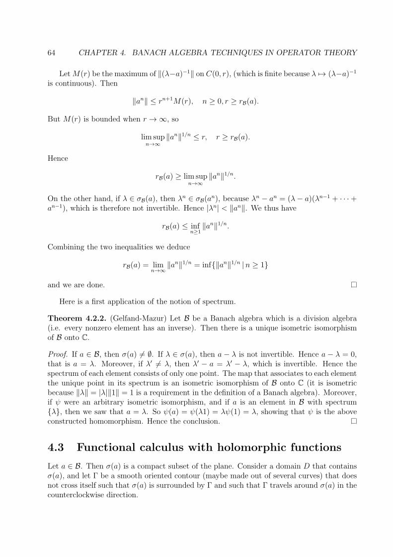
64 CHAPTER 4. BANACH ALGEBRA TECHNIQUES IN OPERATOR THEORY
LetM(r) be the maximum of ‖(λ−a)−1‖ on C(0, r), (which is finite because λ 7→ (λ−a)−1
is continuous). Then
‖an‖ ≤ rn+1M(r), n ≥ 0, r ≥ rB(a).
But M(r) is bounded when r → ∞, so
lim supn→∞
‖an‖1/n ≤ r, r ≥ rB(a).
Hence
rB(a) ≥ lim supn→∞
‖an‖1/n.
On the other hand, if λ ∈ σB(a), then λn ∈ σB(a
n), because λn − an = (λ− a)(λn−1 + · · ·+an−1), which is therefore not invertible. Hence |λn| < ‖an‖. We thus have
rB(a) ≤ infn≥1
‖an‖1/n.
Combining the two inequalities we deduce
rB(a) = limn→∞
‖an‖1/n = inf{‖an‖1/n |n ≥ 1}
and we are done.
Here is a first application of the notion of spectrum.
Theorem 4.2.2. (Gelfand-Mazur) Let B be a Banach algebra which is a division algebra(i.e. every nonzero element has an inverse). Then there is a unique isometric isomorphismof B onto C.
Proof. If a ∈ B, then σ(a) 6= ∅. If λ ∈ σ(a), then a − λ is not invertible. Hence a − λ = 0,that is a = λ. Moreover, if λ′ 6= λ, then λ′ − a = λ′ − λ, which is invertible. Hence thespectrum of each element consists of only one point. The map that associates to each elementthe unique point in its spectrum is an isometric isomorphism of B onto C (it is isometricbecause ‖λ‖ = |λ|‖1‖ = 1 is a requirement in the definition of a Banach algebra). Moreover,if ψ were an arbitrary isometric isomorphism, and if a is an element in B with spectrum{λ}, then we saw that a = λ. So ψ(a) = ψ(λ1) = λψ(1) = λ, showing that ψ is the aboveconstructed homomorphism. Hence the conclusion.
4.3 Functional calculus with holomorphic functions
Let a ∈ B. Then σ(a) is a compact subset of the plane. Consider a domain D that containsσ(a), and let Γ be a smooth oriented contour (maybe made out of several curves) that doesnot cross itself such that σ(a) is surrounded by Γ and such that Γ travels around σ(a) in thecounterclockwise direction.

4.3. FUNCTIONAL CALCULUS WITH HOLOMORPHIC FUNCTIONS 65
For a holomorphic function in D, we have the Cauchy formula
f(z0) =1
2πi
∫
Γ
f(z)(z − z0)−1dz.
Now let us replace z0 by a. Then on Γ, the element (z − a)−1 is defined. With Cauchy’sformula in mind, we can define
f(a) =1
2πi
∫
Γ
f(z)(z − a)−1dz. (4.3.1)
Lemma 4.3.1. The operator f(a) is well defined and does not depend on the contour Γ.
Proof. Because on z 7→ ‖(z− a)−1‖ is continuous on ρ(a) and Γ is a compact subset of ρ(a),it follows that ‖ supΓ(z−a)−1‖ <∞. So the integral can be defined using limits of Riemannsums, which converge by Proposition 4.1.1. Hence the definition makes sense.
Let φ be a continuous linear functional. The function z 7→ f(z)φ((z − a)−1) is holomor-phic. By Cauchy’s theorem, the integral
1
2πi
∫
Γ
f(z)φ((z − a)−1)dz = φ
(
1
2πi
∫
Γ
f(z)(z − a)−1dz
)
does not depend on Γ. So f(a) itself does not depend on Γ.
However, if f(z) =∑
n cnzn is an entire function, then we can define the element
f(a) =∑
n
cnan,
since again the series converges. The integral formula (4.3.1) would be meaningful only if inthis particular situation the two versions coincide. And indeed, we have the following result.
Proposition 4.3.1. If f(z) =∑
n cnzn is a series that converges absolutely in a disk centered
at the origin that contains σ(a), then
∑
n
cnan =
1
2πi
∫
Γ
f(z)(z − a)−1dz
for every oriented contour Γ that surrounds σ(a) counterclockwise.
Proof. Choose N large enough so that∑
n>N |cn|‖a‖n and supΓ
∑
n>N |cnzn| are as small as
we wish. Then we can ignore these sums and consider just the case where f(z) =∑N
n=0 cnzn.
To prove the result in this case, it suffices to check it for f a power of z. Thus let us showthat
an =1
2πi
∫
Γ
zn(z − a)−1dz.
Now we can rely on Cauchy’s theorem about the integral of a holomorphic function, to tomake Γ a circle of radius greater than ‖a‖. Because on Γ |z| > ‖a‖, we can expand
(z − a)−1 =∑
k≥0
ak/kk+1.

66 CHAPTER 4. BANACH ALGEBRA TECHNIQUES IN OPERATOR THEORY
The series on the right is absolutely convergent, so we can integrate term-by-term to write
1
2πi
∫
Γ
zn(z − a)−1dz =∞∑
k=0
1
2πi
(∫
Γ
zn−k−1dz
)
ak.
All of the integrals are zero, except for the one where k = n, which is equal to 2πi. Hencethe result is an, as desired.
A slight modification of the proof yields the following more general result.
Proposition 4.3.2. Suppose R(z) = P (z)/Q(z) is a rational function with poles outside ofthe spectrum of a. Then R(a) is well defined and Q(a) is invertible, and
R(a) = P (a)Q(a)−1.
Theorem 4.3.1. (The Spectral Mapping Theorem for Polynomials) Let P (z) be a polyno-mial and a an element in B. Then
σ(P (a)) = P (σ(a)).
Proof. Let λ ∈ σ(a). Then
P (a)− P (λ) = (a− λ)Q(a).
Because a−λ is not invertible, neither is P (a)−P (λ). Hence P (λ) ∈ σ(P (a)). ConsequentlyP (σ(a)) ⊂ σ(P (a)).
Let λ ∈ σ(P (a)), and let λ1, λ2, . . . , λn be the roots of P (z) = λ. Then
P (a)− λ = (a− λ1)(a− λ2) · · · (a− λn).
Because P (a) − λ is not invertible, there is k such that a − λk is not invertible. Thenλk ∈ σ(a), and λ = P (λk) ∈ P (σ(a)). This proves σ(P (a)) ⊂ P (σ(a)). The double inclusionyields the desired equality.
Theorem 4.3.2. Let D be a domain in C that contains σ(a). Endow the space of holomor-phic functions on D, Hol(D), with the topology of uniform convergence on compact subsets.Then the map Hol(D) → B, f 7→ f(a) is a continuous algebra homomorphism.
Proof. The only difficult step is multiplicativity. But we have multiplicativity for polynomi-als, and hence for rational functions. By Runge’s theorem, every function in Hol(D) is thelimit of rational functions. By passing to the limit in fn(a)gn(a) = (fngn)(a), we concludethat multiplicativity holds in general.
Theorem 4.3.3. (The Spectral Mapping Theorem for Holomorphic Functions) Let f be aholomorphic function in a neighborhood of the spectrum of a. Then
σ(f(a)) = f(σ(a)).

4.4. COMPACT OPERATORS, FREDHOLM OPERATORS 67
Proof. Let λ ∈ σ(a). Then as before f(z)−f(λ) = (z−λ)g(z) with g a holomorphic functionwith the same domain as f . By the previous theorem
f(a)− f(λ) = (a− λ)g(a),
so f(a)− f(λ) is not invertible. Hence f(σ(a)) ⊂ σ(f(a)).For the opposite inclusion, let λ ∈ σ(f(a)). If f(z)− λ is nowhere zero on the spectrum
of a, then g(z) = (f(z)− λ)−1 is defined on the spectrum of a, and then
(f(a)− λ)(f − λ)−1(a) = 1
which cannot happen. So f(z)− λ is zero for some z ∈ σ(a), that is λ ∈ f(σ(a)).
4.4 Compact operators, Fredholm operators
In this section we will construct a Banach algebra which is not the algebra of bounded linearoperators on a Banach space. For this we introduce the notion of a compact operator.
Definition. Let X be a Banach space. An operator K ∈ B(X) is called compact if theclosure of the image of the unit ball is compact.
Example. If R is such that im(R) is finite dimensional, then R is compact. Such an operatoris said to be of finite rank.
Theorem 4.4.1. The set K(X) of compact linear operators on X is a closed two-sided idealof B(X).
Proof. Let K1 and K2 be compact operators. Then K1(B0,1) and K2(B0,1) are compact.Then
(K1 +K2)(B0,1) ⊂ K1(B0,1) +K2(B0,1)
and the latter is compact because is the image through the continuous map (x, y) 7→ x + yof the compact set K1(B0,1 ×K2(B0,1) ⊂ X ×X. This proves that K1 +K2 is compact.
Also for every λ ∈ C, if K is compact then λK is compact, because the image of the setK1(B0,1) through the continuous map x 7→ λx is compact.
Finally, if T ∈ B(X) and K ∈ K(X) then T (K(B0,1)) is the image of a compact setthrough a continuous map, so it is compact. It follows that TK(B0,1) lies inside a compactset, so its closure is compact. So TK is compact.
On the other hand, T (B0,1) is a subset of B0,n for some n, so KT (B0,1) is a closed subset
of the compact set K(B0,n), hence is compact. This proves that KT is compact.We thus showed that K(X) is an ideal. Let us prove that it is closed. Let Kn, n ≥ 1,
be a sequence of compact operators that is norm convergent to an operator T . We wantto prove that T is compact. For this we use the characterization of compactness in metricspaces: “Every sequence contains a convergent subsequence.”

68 CHAPTER 4. BANACH ALGEBRA TECHNIQUES IN OPERATOR THEORY
Let xk, k ≥ 1 be a sequence of points in the unit ball of X. Let us examine the sequenceTxk, n ≥ 1. For every ǫ > 0, there is n(ǫ) such that for n ≥ n(ǫ), ‖Knxk−Txk‖ ≤ ‖Kn−T‖ ≤ǫ. For n ≥ n(ǫ),
‖Txk − Txl‖ ≤ ‖Txk −Knxk‖+ ‖Knxk −Knxl‖+ ‖Knxl − Txl‖ ≤ 2ǫ+ ‖Knxk −Knxl‖.
The sequence Knxk has a convergent subsequence, and so we can find a subsequence Tnxkmsuch that ‖Txkm − Txkr‖ < 3ǫ for all m, r. Do this for ǫ = 1, then choose the first term of asequence yk to be xk1 . Inductively let ǫ = 1/k, and choose from the previous sequence xkma subseqence such that ‖Txkm −Txkr‖ < 3ǫ and let yk be the first term of this subsequence.The result is a Cauchy sequence Tyk, which therefore converges. We conclude that T iscompact.
Theorem 4.4.2. Let K ∈ B(X) be a compact operator. Then
(a) If im(K) is closed, then dimim(K) <∞.
(b) If λ 6= 0, then dimker(K − λI) <∞.
(c) If dimX = ∞, then λ ∈ σ(K).
Proof. (a) If im(K) is closed, then it is a Banach space. The Open Mapping Theoremimplies that the image of the unit ball is a neighborhood of the origin. This neighborhoodis compact, and this only happens if im(K) is finite dimensional.
(b) The operator K|ker(K − λI) is a multiple of the identity operator. This operator isalso compact. By (a) this can only happen if we are in a finite dimensional situation.
(c) The operator K cannot be onto.
Theorem 4.4.3. Let B be a Banach algebra and let M be a two-sided closed ideal. ThenB/M is a Banach algebra with the norm
‖[a]‖ = inf{‖a+m‖ |m ∈ M}.
Here we denote by [a] the image of a under the quotient map.
Proof. Let us show first that ‖ · ‖ is a norm. Clearly if [a] = 0 then a ∈ M so ‖[a]‖ ≤‖a − a‖ = 0. Now assume that ‖[a]‖ = 0. Then There is a sequence mn ∈ M such thatlimn→∞ ‖a+mn‖ = 0. Since M is closed, it follows that a ∈ M, so [a] = 0. Thus ‖[a]‖ = 0if and only if [a] = 0.
If a ∈ B and α ∈ C, then
‖α[a]‖ = ‖[αa]‖ = inf{‖a+ αm‖ |m ∈ M} = |α| inf{‖a+m′‖ |m′ ∈ M} = |α|‖[a]‖.
Also
‖[a] + [b]‖ = ‖[a+ b]‖ = inf{‖a+ b+m‖ |m ∈ M} = inf{‖a+m+ b+m′‖ |m,m′ ∈ M}≤ inf{‖a+ αm‖ |m ∈ M}+ inf{‖a+ αm‖ |m ∈ M} = ‖[a]‖+ ‖[b]‖.

4.5. THE GELFAND TRANSFORM 69
Thus ‖ · ‖ is a norm.Next, let us show that the norm satisfies the requirements from the definition of a Banach
algebra. First,
‖[1]‖ = inf{‖1−m‖ |m ∈ M} = 1,
where the equality is attained for m = 0, and one cannot have ‖1−m‖ < 1 for in that casem must be invertible and hence cannot be an element of an ideal.
Secondly, for a, b ∈ B, we have
‖[a][b]‖ = ‖[ab]‖ = inf{‖ab−m‖ |m ∈ M} ≤ inf{‖(a−m1)(b−m2) |m1,m2 ∈ M}≤ inf{‖a−m1‖ |m1 ∈ M} inf{‖b−m2‖ |m2 ∈ M} = ‖[a]‖‖[b]‖.
Finally, let us show that B/M is complete. Showing that every Cauchy sequence isconvergent is equivalent to showing that every absolutely convergent series is convergent. Itis clear that the fact that every Cauchy sequence is convergent implies that every absolutelyconvergent series is convergent. For the converse, let xn, n ≥ 1 be a Cauchy sequence. Bychoosing a subsequence, we may assume that |yn − ym| ≤ 1/2k whenever n,m ≥ k. Setxk = yk+1 − yk. Then
∑
xk is absolutely convergent, and its sum is the limit of yk.So let
∑
n[an] be a series such that∑
n ‖[an]‖ = M < ∞. Then for each n there is mn
sucht that ‖an + mn‖ ≤ ‖an‖ + 1/2n. Hence∑
n(an + mn) is absolutely convergent, andtherefore convergent in B. If a is its sum, then a + M is the sum of the original series inB/M. This concludes the proof that B/M is a Banach algebra.
Corollary 4.4.1. The algebra B(X)/K(X) is a Banach algebra.
Definition. The algebra B(X)/K(X) is called the Calkin algebra.
Definition. An operator with finite dimensional kernel and with closed image of finitecodimension is called Fredholm.
Theorem 4.4.4. (Atkinson) Let H be a Hilbert space. Then the Fredholm operators formthe preimage through the quotient map of the invertible elements of B(H)/K(H).
Corollary 4.4.2. The Fredholm operators form an open set.
Definition. If T is Fredholm, then the index of T is
ind(T ) = dimker(T )− codim im(T ) = codim im(T ∗)− dimker(T ∗).
One can show that the index is continuous and invariant under compact perturbations.
4.5 The Gelfand transform
Definition. Let B be a Banach algebra. A complex linear functional φ on B is said to bemultiplicative if(a) φ(ab) = φ(a)φ(b) for all a, b,(b) φ(1) = 1.

70 CHAPTER 4. BANACH ALGEBRA TECHNIQUES IN OPERATOR THEORY
We denote the set of all multiplicative functionals by MB.
Proposition 4.5.1. If B is a Banach algebra and φ ∈MB, then ‖φ‖ = 1.
Proof. Since φ(a − φ(a)) = 0 it follows that every element in B is of the form λ + a, forsome λ ∈ C and a ∈ ker(φ). Note that if λ 6= 0 and ‖λ + a‖ < |λ| = |φ(λ + a)|, then a isinvertible. This cannot happen, because φ(a) = 0 implies 1 = φ(aa−1) = φ(a)φ(a−1) = 0.Hence |φ(b)| ≤ ‖b‖ for all b. Because φ(1) = 1, the equality is attained, so ‖φ‖ = 1.
Proposition 4.5.2. MB is a compact subspace of X∗ endowed with the weak∗ topology.
Proof. As a corollary of the previous proposition, MB is a subset of the unit ball in X∗.Because of the Banach-Alaoglu theorem, all we have to show is that MB is weak∗-closed.This amounts to showing that if a linear functional is in the weak∗-closure of this set, thenit is multiplicative.
Assume φ(1) 6= 1, and let ǫ < |φ(1)− 1|. If ψ ∈MB ∩ V (1, ǫ), then
ǫ < |φ(1)− 1| = |φ(1)− ψ(1)| < ǫ.
This is impossible, so φ(1) = 1.Similarly, if φ(ab) 6= φ(a)φ(b) for some a, b (which we may assume to lie in the unit ball),
choose ǫ = |φ(ab)− φ(a)φ(b)|, and ψ ∈ V (a, b, ab, ǫ/3). Then
ǫ < |φ(ab)− φ(a)φ(b)| = |φ(ab)− ψ(ab) + ψ(ab)− ψ(a)ψ(b) + ψ(a)ψ(b)− φ(a)φ(b)|≤ |φ(ab)− ψ(ab)|+ |φ(a)φ(b)− ψ(a)ψ(b)| ≤ ǫ/3 + |φ(a)φ(b)− φ(a)ψ(b) + φ(a)ψ(b)− ψ(a)ψ(b)|≤ ǫ/3 + |φ(a)||φ(b)− ψ(b)|+ |ψ(b)||φ(a)− ψ(a)| < ǫ/3 + ǫ/3 + ǫ/3 = ǫ.
Again this is impossible, so φ is multiplicative.
Proposition 4.5.3. If B is a commutative Banach algebra, then MB is in one-to-one corre-spondence with the set of maximal two-sided ideals in B.
Proof. The correspondence is φ 7→ ker(φ).So first, let us show that if φ is a multiplicative linear functional, then ker(φ) is a maximal
two-sided ideal. That it is an ideal follows from φ(a) = 0 → φ(ab) = φ(a)φ(b) = 0. It ismaximal because every element in B is of the form λ + a where a ∈ ker(φ). If a were in anideal and λ+a were in an ideal, then λ and hence 1 would be in an ideal, which is impossible.Hence the kernel is maximal.
Conversely, let M be a maximal two-sided ideal. We will prove that there is φ ∈ MB
such that ker(φ) = M. Because if a ∈ M, then a is not invertible, then ‖1− a‖ ≥ 1, so 1 isnot in the closure of M. Thus the closure of M is an ideal, and because of maximality, thisideal must be M. So M is closed.
The quotient algebra B/M is a division algebra, because M is maximal. So by theGelfand-Mazur Theorem it is C. The quotient map is the desired multiplicative functional.
Recall that for every a ∈ B, the function a : (B∗)1 → C given by a(φ) = φ(a) is continuous,where (B∗)1 is the unit ball in B∗, endowed with the weak∗ topology.

4.5. THE GELFAND TRANSFORM 71
Definition. The Gelfand transform of the Banach algebra B is the function Γ : B → C(MB)given by Γ(a) = a|MB.
Theorem 4.5.1. The Gelfand transform is an algebra homomorphism and ‖Γ(a)‖ ≤ ‖a‖for all a ∈ B.
Proof. Γ is clearly linear and Γ(1) = 1. Let us check that Γ is multiplicative. We have
[Γ(ab)](φ) = φ(ab) = φ(a)φ(b) = [Γ(a)](φ)[Γ(b)](φ) = [Γ(a)Γ(b)](φ).
Next, let us check that Γ is contractive. We have
‖Γ(a)‖ = sup{|φ(a)| |φ ∈MB} ≤ sup{‖φ‖‖a‖ |φ ∈MB} = ‖a‖.
If B is not commutative, the Gelfand transform has large kernel which is generated bythe elements of the form ab− ba. For this reason it is not so interesting.
Proposition 4.5.4. If B is a commutative Banach algebra and a ∈ B, then a is invertiblein B if and only if Γ(a) is invertible in C(MB).
Proof. If a is invertible, then Γ(a−1) = (Γ(a))−1. If a is not invertible, thenM0 = {ab | b ∈ B}is a proper ideal. It is contained in a maximal ideal, whose associated functional is zero ona. Hence Γ(a) is not invertible.
Remark 4.5.1. The fact that a invertible implies Γ(a) invertible does not use the fact thatthe Banach algebra is commutative. Because Γ(ab−ba) = Γ(a)Γ(b)−Γ(b)Γ(a) = 0, it followsthat ab− ba is not invertible. This means that the canonical commutation relations for theposition and momentum operators in quantum mechanics
PQ−QP =~
iI
cannot be modeled with bounded linear operators.
Proposition 4.5.5. If B is a commutative Banach algebra and a ∈ B, then σB(a) = im(Γ(a))and rB(a) = ‖Γ(a)‖.
Proof. If λ is not in σ(a), then a−λ is invertible. This is equivalent to Γ(a)−λ is invertible.And this is further equivalent to the fact that λ is not in the image of Γ(a).

72 CHAPTER 4. BANACH ALGEBRA TECHNIQUES IN OPERATOR THEORY

Chapter 5
C∗ algebras
5.1 The definition of C∗-algebras
Again, most of this chapter is from the book of Ronald Douglas.
Definition. A C∗-algebra is a Banach algebra over the complex numbers with an involution∗ that satisfies
• (a+ b)∗ = a∗ + b∗
• (λa)∗ = λa∗
• (ab)∗ = b∗a∗
• (a∗)∗ = a.
Additionally, the involution should satisfy
‖a∗a‖ = ‖a‖‖a∗‖. (5.1.1)
Alternatively, the involution should satisfy
‖a∗a‖ = ‖a‖2. (5.1.2)
The two conditions (5.1.1) and (5.1.2) are equivalent, though it is hard to show that(5.1.1) implies (5.1.2). Thus our working definition will be the one with (5.1.2), what isusually called a B∗-algebra. This condition implies (5.1.1) as follows:
‖x‖2 = ‖x∗x‖ ≤ ‖x‖‖x∗‖.
Hence ‖x‖ ≤ ‖x∗‖ and ‖x∗‖ ≤ ‖(x∗)∗‖ = ‖x‖. So ‖x‖ = ‖x∗‖. Then ‖x∗x‖ = ‖x‖2 =‖x‖‖x∗‖. From these calculations we conclude that in a C∗ algebra the involution is anisometry.
Example. The algebra B(H) of bounded linear operators on a Hilbert space with the invo-lution defined by taking the adjoint.
73

74 CHAPTER 5. C∗ ALGEBRAS
Example. Let X be a compact Hausdorff space. The algebra C(X) of complex valuedcontinuous linear functions on X with the sup norm and the involution given by (f ∗)(x) =f(x) is a C∗-algebra.
Example. The algebra K(H) of compact operators on a Hilbert space H is a C∗-algebra.We know that it is a subalgebra of B(H), so all we have to check is that it is closed undertaking the adjoint. Thus we have to show that the adjoint of a compact operator is compact.
Let T be compact and consider a sequence yn, n ≥ 1 in the unit ball B0,1 centered atthe origin of H. Let us prove that T ∗yn has a convergent subsequence. Define the functionsfn : T (B0,1) → C,
fn(x) = 〈x, yn〉where 〈·, ·〉 is the inner product. Note that since T is compact, the domain of these functionsis compact. Then
|fn(x)| ≤ ‖x‖‖yn‖ ≤ 1.
So ‖fn‖, n ≥ 1 is a bounded sequence. Also,
|fn(x)− fn(x′)| ≤ ‖yn‖‖x− x′‖ ≤ ‖x− x′‖,
so the sequence fn is also equicontinuous. By the Arzela-Ascoli theorem, it has a convergentsubsequence in C(T (B0,1)). Note also that
‖fn‖ = sup{|fn(x)| | x ∈ T (B0,1)} = sup{| 〈Tx, yn〉 | | x ∈ B0,1} = sup{| 〈x, T ∗yn〉 | | x ∈ B0,1}= ‖T ∗yn‖.
Thus T ∗yn has a norm convergent subsequence, showing that T ∗ is compact.
Definition. If B and B′ are C∗-algebras then f : B → B′ is called a homomorphism if it isan algebra homomorphism and f(a∗) = f(a)∗ for all a.
An element a is called self-adjoint if a = a∗, normal if aa∗ = a∗a and unitary if aa∗ =a ∗ a = 1.
Theorem 5.1.1. In a C∗-algebra the spectrum of a unitary element is contained in the unitcircle, and the spectrum of a self-adjoint element is contained in the real axis.
Proof. If u is unitary, then 1 = ‖1‖ = ‖u∗u‖ = ‖u2‖, so ‖u‖ = ‖u∗‖ = ‖u−1‖ = 1. Thenif |λ| > 1, then λ − u is invertible. Also, if |λ| < 1, then 1 − λu−1 is invertible, and so is−u(1− λu−1) = λ− u. Hence
σB(u) ⊂ {λ ∈ C | |λ| < 1}.Let B be the C∗-algebra. If a ∈ B is self-adjoint, then u = exp(ia) is unitary. Indeed,
u∗ = exp(ia)∗ = exp(−ia), anduu∗ = exp(ia) exp(−ia) = exp(ia− ia) = 1 = u∗u.
Because σB(u) is a subset of the unit disk, and, by the Spectral Mapping Theorem, σ(u) =exp(iσ(a)), the spectrum of a must be real.

5.2. COMMUTATIVE C∗-ALGEBRAS 75
5.2 Commutative C∗-algebras
Theorem 5.2.1. (Gelfand-Naimark) If B is a commutative C∗-algebra and MB is the set ofmultiplicative functionals on B, then the Gelfand transform is a ∗-isometrical isomorphismof B onto C(MB).
Proof. Let us show that Γ is a ∗-map. If a ∈ B, then b = 12(a + a∗) and c = 1
2i(a − a∗) are
self-adjoint operators such that a = b + ic and a∗ = b− ic. Recall that σB(b) and σB(c) aresubsets of R, by Theorem 5.1.1. By Proposition 4.5.5, the functions Γ(b) and Γ(c) are realvalued. Hence
Γ(a) = Γ(b) + iΓ(c) = Γ(b)− iΓ(c) = Γ(a∗).
This shows that Γ is a homomorphism of C∗-algebras.Let us show that it is an isometry. We have
‖a‖2 = ‖a∗a‖ = ‖(a∗a)2n‖1/2n = limn→∞
‖(a∗a)2n‖1/2n = rB(a∗a).
By Proposition 4.5.5, this is equal to the sup norm of Γ(a∗a). We have
‖Γ(a∗a)‖ = ‖Γ(a∗)Γ(a)‖ = ‖Γ(a)2‖ = ‖Γ(a)‖2.
Hence ‖a‖ = ‖Γ(a)‖, as desired.Finally, if φ and ψ are multiplicative functionals, then Γ(a)(φ) = Γ(a)(ψ) for all a means
that φ(a) = ψ(a) for all a, hence φ = ψ. This shows that the functions in the imageof Γ separate points. The image contains the identity function, and for each function itcontains its complex conjugate. So by the Stone-Weierstrass theorem, they are all continuousfunctions on MB.
Theorem 5.2.2. (The Spectral Theorem) If H is a Hilbert space and N is a normal operatoron H, then the C∗-algebra CN generated by N and N∗ is commutative. Moreover, themaximal ideal space of CN is homeomorphic to σ(N) and hence the Gelfand map is a ∗-isometrical isomorphism of CN onto C(σ(N)).
Proof. The algebra CN is commutative because it is the closure of the algebra of all polyno-mials in N and N∗.
Let us show that the set of multiplicative functionals, MCN , is homeomorphic to σ(N).In view of Proposition 4.5.5, we can define the onto function
Ψ :MCN → σ(N), Ψ(φ) = Γ(N)(φ).
This function is also one-to-one, because if Ψ(φ) = Ψ(φ′), then
φ(N) = Γ(N)(φ) = Γ(N)(φ′) = φ′(N),
and also
φ(N∗) = Γ(N∗)(φ) = Γ(N)(φ) = Γ(N)(φ′) = Γ(N∗)(φ′) = φ′(N∗).

76 CHAPTER 5. C∗ ALGEBRAS
Hence φ and φ′ coincide on CN , so they are equal.Finally, let us show that Ψ is continuous. Let
Bλ0,r = {λ ∈ σ(N) | |λ− λ0| < r}.
Set φλ0= Ψ−1(λ0). Then
Ψ−1(Bλ0,r) = {φ ∈MCN | |φ(N)− φλ0(N)| < r},
which is open in the weak∗ topology. Hence Ψ is continuous.Because MCN and σ(N) are compact Hausdorff spaces, Ψ is a homeomorphism.
5.3 C∗-algebras as algebras of operators
Definition. Given a C∗-algebra B, a ∗-representation is a (continuous) C∗-homomorphism
ρ : B → B(H),
for some Hilbert space H, that is non-degenerate in the sense that ρ(a)x is dense when aranges through a and x ranges throughH. A vector x is called cyclic if the set {ρ(a)x | a ∈ B}is dense in H; in this case the representation is called cyclic.
Definition. A state on a C∗-algebra is a linear functional φ such that φ(a∗a) ≥ 0 for all aand ‖φ‖ = 1.
Note that a state φ has the property that φ(1) = 1.
Theorem 5.3.1. (The Gelfand-Naimark-Segal Construction) Given a state φ of B, there isa ∗-representation ρ : B → B(H) which is cyclic, and a cyclic vector x such that
φ(a) = 〈ρ(a)x, x〉 for all a ∈ B.
Proof. Let a ∈ B act on the left on B by
ρφ(a)b = ab.
This is the left regular representation. We want this to be a representation on a Hilbertspace, and for that reason we attempt to turn B into a Hilbert space. We define the innerproduct by
〈a, b〉 = φ(b∗a).
This has all the nice properties of an inner product, except that it might be degenerate, inthe sense that there might be a such that 〈a, a〉 = φ(a∗a) = 0. Adapting the Cauchy-Schwarzinequality, we deduce that the set Nφ of elements a such that 〈a, a〉 = 0 form a subspace ofB.
Let us show that Nφ is also a left ideal of B. This is because of the Cauchy-Schwarzinequality:
|φ((a∗b∗ba)|2 ≤ φ(a∗a)φ((b∗ba)(a∗b∗b)) = 0.

5.4. FUNCTIONAL CALCULUS FOR NORMAL OPERATORS 77
Then B/Nφ is an inner product space. Consider the completion Hφ of this space, whichis therefore a Hilbert space. We have
‖a‖2b∗b− b∗a∗ab = b∗(‖a‖2 − a∗a)b = b∗c∗cb,
where
c = c∗ = (‖a‖2 − a∗a)1/2 = (‖a∗a‖ − a∗a)1/2.
The element c can by defined because the function f(t) = (‖a∗a‖ − a∗a)1/2 is continuous onσ(a∗a), so we can use Theorem 5.2.2. So, because φ is positive,
φ(b∗a∗ab) ≤ φ(‖a‖2b∗b) = ‖a‖2φ(b∗b).
It follows that
‖a(b+Nφ)‖Hφ≤ ‖a‖2‖b+Nφ‖Hφ
,
so ρφ(a) is continuous. This implies that ρφ(a) can be extended to the entire Hilbert spaceHφ. This representation is cyclic, with cyclic vector 1 + Nφ. Also, 〈ρφ(a)1, 1〉 = φ(1∗a1) =φ(a).
The set of states is a weak∗ closed convex subset of the unit ball of B∗. The extremalpoints are called pure states.
Theorem 5.3.2. (Gelfand-Naimark) Every C∗-algebra admits an isometric ∗-representation.If the C∗-algebra is separable, then the Hilbert space can be chosen to be separable as well.
Proof. Consider the set of pure states and define
ρ : B → ⊕φB(Hφ), ρ = ⊕ρφ
where the sum is taken over all pure states. It suffices to show that ρ is faithful, namelyone-to-one, because the fact that it is an isometric ∗-homomorphsm then follows from The-orem 5.4.3 proved in next section. For this we use the theorem of M. Riesz about extensionof positive functionals. Let a be a nonzero element of B. Then there is a state φ such thatφ(a∗a) > 0.
Consider the GNS representation associated to φ, and let x be its cyclic vector. Then
‖ρφ(a)x‖2 = 〈ρφ(a)x, ρφ(a)x〉 = 〈ρφ(a∗a)x, x〉 = φ(a∗a) > 0.
By the Krein-Milman theorem, there is a pure state φ that satisfies φ(a∗a) > 0. In this caseρφ 6= 0, hence the representation is faithful. The theorem is proved.
5.4 Functional calculus for normal operators
Throughout this section we assume that the Hilbert space H is separable.

78 CHAPTER 5. C∗ ALGEBRAS
Definition. Let H be a Hilbert space. The weak operator topology is the topology definedby the open sets
V (T0; x1, x2, . . . , xk; y1, y2, . . . , yk; r) = {T ∈ B(H) | | 〈(T − T0)xj, yj〉 | < r, j = 1, 2, . . . , k}.
The strong operator topology is the topology defined by the open sets
V (T0; x1, x2, . . . , xk; r) = {T ∈ B(H) | ‖(T − T0)xj‖ < r, j = 1, 2, . . . , k}.
Definition. A von Neumann algebra is a C∗-subalgebra of B(H) that is weakly closed.
Remark 5.4.1. If C is a self-adjoint subalgebra of B(H), then its weak closure is a vonNeumann algebra. If C is commutative, then its closure is commutative.
Proposition 5.4.1. If N is a normal operator on H, then the von Neumann algebra WN
generated by N is commutative. IfMWNis the set of multiplicative functionals on WN , then
the Gelfand transform is a ∗-isometrical isomorphism of WN onto C(MWN).
We want to show that there is a unique L∞ space structure on MWNand a unique ∗-
isometrical isomorphism Γ∗ : WN → L∞(σ(N)) which extends the functional calculus withcontinuous functions defined by the Spectral Theorem (Theorem 5.2.2).
Assume we have a finite positive regular Borel measure on MWN. We can assume that
the measure of the entire space is 1, so that we have a probability measure. For the moment,we work in this hypothesis.
The map φ 7→ Mf , where Mf : L2(MWN) → L2(MWN
), Mfg = fg identifies L∞(MWN)
with a maximal commutative von Neumann subalgebra of the algebra of operators onL2(MWN
).
Proposition 5.4.2. The weak operator topology and the weak∗ topology on L∞ coincide.
Proof. L∞ = L∗1, and recall that every function in L1 is the product of two L2 functions.
Thus an element of the form
φ(f) =
∫
fg
with f ∈ L∞ and g ∈ L1, can also be represented as
∫
Mfg1g2 = 〈Mfg1, g2〉
where g = g1g2. Hence the conclusion.
Proposition 5.4.3. The space C(σ(N)) is weak∗-dense in L∞(σ(N)).
Proof. We will show that the unit ball in C(σ(N)) is weak∗-dense in the unit ball inL∞(σ(N)). Consider a step function in the unit ball of L∞, f =
∑
αjχEj, |αj| ≤ 1 with Ej
disjoint and their union is σ(N)). For each j, choose Kj ⊂ Ej. Using Tietze’s Extension

5.4. FUNCTIONAL CALCULUS FOR NORMAL OPERATORS 79
Theorem we can find g in the unit ball of C(σ(N)) such that g(x) = αj for x ∈ Kj. Thenfor h ∈ L1,
∣
∣
∣
∣
∫
h(f − g)
∣
∣
∣
∣
≤∫
|h||f − g|
=n∑
j=1
∫
Ej\Kj
|h||f − g| ≤n∑
j=1
∫
Ej\Kj
|h|
Because the measure is regular, we can choose Kj such that the integrals are as small asdesired.
Recall that a vector x is cyclic for an algebra B ⊂ B(H) if Bx is dense in H and separatingif Tx = 0 implies T = 0. If B is commutative, then x cyclic implies x separating, becauseTx = 0 implies Bx ∈ ker(T ), hence T = 0.
Theorem 5.4.1. If N is a normal operator on H such that CN has a cyclic vector, thenthere is a positive regular Borel measure ν supported on σ(N) = MCN and an isometricalisomorphism γ from H onto L2(σ(N), ν) such that the map
Γ∗ : WN → B(L2(σ(N), ν), Γ∗(T ) = γTγ−1
is a ∗-isometrical isomorphism from WN onto L∞(σ(N), ν). Moreover, Γ∗ is an extension ofthe Gelfand transform Γ : CT → C(σ(N)). Lastly, if ν1 is a positive regular Borel measureon σ(N) and Γ∗
1 us a ∗-isometrical isomorphism from WN that extends Γ, then ν and ν1 aremutually absolutely continuous, L∞(σ(N), ν) = L∞(σ(N), ν1) and Γ∗
1 = Γ∗.
Proof. Let x be a cyclic vector for CN with ‖x‖ = 1. Consider the linear functional onC(σ(N)) defined by φ(f) = 〈f(N)x, x〉. Then φ is positive because if f ≥ 0 then f = g2 forsome real valued function g, and then
f(N) = g(N)g(N) = g(N)g(N) = (g(N))∗g(N),
and hence
〈f(N)x, x〉 = 〈g(N)x, g(N)x〉 = ‖g(N)x‖2 ≥ 0.
We also have
|φ(f)| = | 〈f(N)x, x〉 | ≤ ‖f(N)‖‖x2‖ = ‖f‖,
thus φ is continuous. By the Reisz Representation Theorem (Theorem 2.1.2), there is apositive regular measure ν on σ(N) such that
∫
σ(N)
fdν = 〈f(N)x, x〉 for f ∈ C(σ(N)).
If the support of ν were not the entire spectrum, then, by Urysohn’s lemma, we could finda continuous function f that is 1 somewhere on the spectrum and is zero on the support of

80 CHAPTER 5. C∗ ALGEBRAS
ν. Then because f is not identically equal to zero, f(N) 6= 0 and because x is separating,we have
0 6= ‖f(N)x‖2 = 〈f(N)x, f(N)x〉 =⟨
|f |2(N)x, x⟩
=
∫
σ(N)
|f |2dν = 0,
impossible. So supp(ν) = σ(N).Define
γ0 : CNx→ L2(σ(N), ν), γ0(f(T )x) = f.
The computation
‖f‖22 =∫
σ(N)
|f |2dν =⟨
|f |2(N)x, x⟩
= ‖f(N)x‖2
shows that γ0 is a Hilbert space isometry. Because CN is dense in H and C(σ(N)) is densein L2(σ(N), ν), γ0 can be extended uniquely to an isometrical isomorphism
γ : H → L2(σ(N), ν).
Moreover, if we define
Γ∗ : WN → B(L2(σ(N), ν)), Γ∗(T ) = γTγ−1
then Γ∗ is a ∗-isometrical isomorphism onto the image.Let us show that Γ∗ extends the Gelfand transform
Γ : CN → B(L2(σ(N), ν)).
Indeed, if f ∈ C(σ(N)), then for all g ∈ C(σ(N)),
[Γ∗(f(N))]g = γf(N)γ−1g = γf(N)g(N)x = γ[(fg)(N)x] = fg =Mfg.
Since C(σ(N)) is dense in L2(σ(N), ν), it follows that
Γ∗(f(N)) =Mf = Γ(f(N)).
Because the weak operator topology and the weak∗ topology coincide on L∞ (Proposi-tion 5.4.2), Γ∗ is a continuous map fromWT with the weak operator topology to L∞(σ(N), ν)with the weak∗ topology. And because continuous functions are weak∗-dense in L∞, it fol-lows that Γ∗(WT ) = L∞(σ(N), ν). Thus Γ∗ is a ∗-isometrical isomorphism mapping WT ontoL∞(σ(N), ν).
Finally, if (ν1,Γ1) are a different pair with the above properties, then Γ∗Γ∗1−1 is a
∗-isometrical isomorphism from L∞(σ(N), ν1) onto L∞(σ(N), ν) which is the identity onC(σ(N)). Then ν and ν1 are mutually absolutely continous, L∞(σ(N)ν) = L∞(σ(N), ν1)and Γ∗Γ∗−1
1 is the identity. This completes the proof.

5.4. FUNCTIONAL CALCULUS FOR NORMAL OPERATORS 81
However, not all operators have cyclic vectors. Instead we will use non-separating vectorsand replace H by the smallest invariant subspace containing a non-separating vector. Weproceed to show that every normal has a separating vector.
An easy application of Zorn’s lemma yields the following result.
Proposition 5.4.4. Every commutative C∗-algebra is contained in a maximal commutativevon Neumann algebra.
Definition. If A ⊂ L(H), then the commutant of A, denoted A′, is the set of operators inL(H) which commute with every operator in A.
Proposition 5.4.5. A C∗-algebra in L(H) is a maximal commutative von Neumann algebraif and only if it is equal to its own commutant.
Proof. Let B be the C∗-algebra. If B is commutative, then B ⊂ B′. If B is maximalcommutative then necessarily we have equality.
Conversely, if equality holds, then B is a von Neumann algebra. It must be maximalcommutative, for if A commutes with everything in B, then A ∈ B′ = B.
Lemma 5.4.1. Let T ∈ B(H), V is a closed subspace ofH, and PV the orthogonal projectiononto V . Then PV T = TPV if and only if V is an invariant subspace for both T and T ∗.Moreover, in this case both V and V ⊥ are invariant for T .
Proof. V is invariant for T if and only if PV TPV = TPV . So V is invariant for both T and T ∗
if and only if PV TPV = TPV and PV T∗PV = T ∗PV . The latter is equivalent, by conjugating
to PV TPV = PV T . So V is invariant for both T and T ∗ if and only if PV T = TPV (in whichcase the equality to PV TPV is superfluous). Note also that V invariant for T∗ implies V ⊥
invariant for T (by the equality 〈Tx, y〉 = 〈x, T ∗y〉).
Definition. A subspace V ofH is a reducing subspace for T if it satisfies any of the equivalentconditions from the statement of the above lemma.
Lemma 5.4.2. If B is a C∗-algebra contained in B(H) and v ∈ H, then the projection ontoBv is in B′.
Proof. By Lemma 5.4.1, it suffices to show that Bv is invariant for both T and T ∗ for everyT ∈ B. Note that T ∗ ∈ B so both T and T ∗ leave Bv invariant.
Theorem 5.4.2. If B is a maximal commutative von Neumann algebra on a separableHilbert space H, then B has a cyclic vector.
Proof. Let E be the set of all collections of projections {Eα}α∈A in B such that
• For each α ∈ A there is vα ∈ H\{0} so that Eα is the projection onto Bvα
• EαEα′ = Eα′Eα = 0 for α 6= α′.

82 CHAPTER 5. C∗ ALGEBRAS
Clearly E is not empty, since we can build an element in E starting with one vector, viaLemma 5.4.2. Order E by inclusion. The hypothesis of Zorn’s Lemma is satisfied. Pick amaximal element {Eα}α∈A.
Let F be the collection of all finite subsets of the index set A partially ordered by inclusionand let {PF}F∈F be the net of the orthgonal projections defined by
PF =∑
α∈F
Eα.
Then the net is increasing. If F > F ′ then
‖(PF − PF ′)x‖2 =⟨
(PF − PF ′)2x, x⟩
= 〈(PF − PF ′)x, x〉 = 〈PFx, x〉 − 〈PF ′x, x〉 .The net 〈PFx, x〉 is increasing and bounded from above by ‖x‖2, so it is convergent. Henceit is Cauchy, and so is ‖PFx‖. Then PFx is norm convergent. Define Px = limF PFx. ThenP is an orthgonal projection.
The range V of P has the property that both V and V ⊥ are invariant under B. MoreoverP ∈ B by Lemma 5.4.2. Note that if v ∈ V ⊥, then Bv is orthogonal to each Eα so we canadd the projection onto this space to the family {Eα}α, contradicting maximality. HenceV ⊥ = 0.
Because H is separable, A is countable. Thus we can define w =∑
α vα. Then for eachα, the range of Eα is contained in Bw. So w is a cyclic vector for B.Corollary 5.4.1. Every commutative C∗-algebra of operators on a separable Hilbert spacehas a separating vector.
Theorem 5.4.3. If Φ : B1 → B2 is a ∗-homomorphism of C∗-algebras, then ‖Φ‖ ≤ 1 and Φis an isometry if and only if it is one-to-one.
Proof. If a ∈ B1 and a = a∗ (i.e. a is self-adjoint), then Ca is a commutative C∗-algebra con-tained in B1 and Φ(Ca) is a commutative C∗-algebra contained in B2. If φ is a multiplicativelinear functional on Φ(Ca), then φ ◦Φ is a multiplicative linear functional on Ca. Because ofthe Gelfand-Naimark Theorem, we can choose φ so that |φ(Φ(a))| = ‖Φ(a)‖. Then
‖a‖ ≥ |φ(Φ(a))| = ‖Φ(a)‖,so Φ is a contraction on self-adjoint elements. For arbitrary b ∈ B1,
‖b‖2 = ‖b∗b‖ ≥ ‖Φ(b∗b)‖ = ‖Φ(b)∗Φ(b)‖ = ‖Φ(b)‖2.Hence ‖Φ‖ ≤ 1.
For the second part, clearly if Φ is an isometry than it is one-to-one. Assume that Φ isnot an isometry and choose b such that ‖b‖ = 1 but ‖Φ(b)‖ < 1. Set a = b∗b; then ‖a‖ = 1but ‖Φ(a)‖ = 1 − ǫ with ǫ > 0. Choose a function f ∈ C([0, 1]) such that f(1) = 1 andf(x) = 0 if 0 ≤ x ≤ 1− ǫ. Using the functional calculus on Ca, define f(a). Since
σ(f(a)) = im(Γ(f(a)) = f(σ(a)),
we conclude that 1 ∈ σ(f(a)), so f(a) 6= 0. We have Φ(f(a)) = f(Φ(a)) (true on polynomialsthen pass to the limit). But ‖Φ(a)‖ = 1 − ǫ, so σ(Φ(f(a)) ⊂ [0, 1 − ǫ]. Hence Φ(f(a)) =f(Φ(a)) = 0. Thus Φ is not one-to-one.

5.4. FUNCTIONAL CALCULUS FOR NORMAL OPERATORS 83
Let H be a separable Hilbert space and N normal on H. By Corollary 5.4.1, the com-mutative von Neumann algebra WN has a separating vector x. If we set Hx = WNx, thenboth Hx and H⊥
x are invariant under WN . We can therefore define a map Φ : WN → B(Hx)by Φ(N) = N |Hx.
Lemma 5.4.3. The map Φ defined above is a ∗-isometrical isomorphism. Moreover σB(H)(T ) =σB(Hx)(T |Hx) for all T ∈ WN .
Proof. In view of the previous theorem, let us show that Φ is one-to-one. And indeed, ifΦ(T ) = 0 then Tx = 0, because x = Ix ∈ WNx. So T = 0, because x is separating of WN .The equality of spectra is proved as follows.
First,
σB(H)(T ) = σWN(T ).
Indeed, σB(H)(T ) ⊂ σWN(T ) because the inverse of λ − T might or might not be in WN .
Moreover, because the resolvent is open both for B(H) and for WN , σWN(T ) is obtained
from σB(H)(T ) by adding to it some bounded components of its complement. So if T − λ isinvertible in B(H), then (T − λ)(T ∗ − λ) is self-adjoint, so its spectrum is real and hencenecessarily the same in B(H) and WN . So this operator must be invertible in WN , and henceso is T − λ. Next
σWN(T ) = σΦ(WN )(T |Hx)
because Φ is a ∗-isometrical isomorphism onto the image. Repeating the above argument wealso have
σΦ(WN )(T |Hx) = σB(Hx)(T |Hx)
and we are done.
Theorem 5.4.4. (Functional Calculus for Normal Operators - Version I) Let N be a normaloperator on the separable Hilbert space H let the Γ : CN → C(σ(N)) be the Gelfandtransform. Then there is a positive regular Borel measure ν having support σ(N) and a∗-isometrical isomorphism Γ∗ from WN onto L∞(σ(N), ν) which extends Γ. Moreover ν isunique up to mutual absolute continuity while L∞(σ(N), ν) and Γ∗ are unique.
Proof. Let x be a separating vector for WN , Hx = WNx, and
Φx : WN → B(Hx), Φx(T ) = T |Hx.
Let Wx be the von Neumann algebra generated by T |Hx. The map Φ is continuous in theweak operator topology (because it is obtained by restricting the domain). Hence Φ(WN) ⊂Wx. Moreover, if
Γ0 : CN |Hx→ C(σ(N))
is the Gelfand transform, then Γ = Γ0 ◦ Φ.

84 CHAPTER 5. C∗ ALGEBRAS
Because N |Hx is normal and has the cyclic vector x, by Theorem 5.4.1 there is a positiveregular Borel measure ν with support σ(N |Hx) = σ(N) (here we use the previous lemma),and a ∗-isometrical (onto) isomorphism
Γ∗0 : Wx → L∞(, σ(N), ν), such that Γ∗
0|CN |Hx= Γ.
Moreover, Γ∗0 is continuous form the weak operator topology of Wx to the weak∗-topology on
L∞(σ(N), ν). Hence Γ∗ = Γ∗0 ◦Φ is a ∗-isometrical isomorphism from WN into L∞(σ(N), ν),
continuous in the weak/weak∗ topologies, and which extends the Gelfand transform.The only thing that remains to show is that Γ∗ takes WN onto L∞(σ(N), ν). For this we
need the following result.
Lemma 5.4.4. Let H be a Hilbert space. Then the unit ball of B(H) is compact in theweak operator topology.
Proof. The proof is from the book of Kadison and Ringrose, Fundamental of the theory ofoperator algebras. For two vectors x, y ∈ H, let Dx,y be the closed disk of radius ‖x‖ · ‖y‖in the complex plane. The mapping which assigns to each T ∈ (B(H))1 the point
{〈Tx, y〉 | x, y ∈ H} ⊂∏
x,y
Dx,y
is a homeomorphism of (B(H))1 with the weak operator topology onto its image X in thetopology induced on X by the product topology of
∏
x,yDx,y. As the latter is a compactHausdorff topology by Tychonoff’s theorem, X is compact if it is closed. So let us provethat X is closed.
Let b ∈ X. Choose x1, y2, x2, y2 ∈ H. Then for every ǫ > 0 there is T ∈ (B(H))1 suchthat each of
|a · b(xj, yk)− a 〈Txj, yk〉 , |b(xj, yk)− 〈Txj, yk〉 |,|b(ax1 + x2, yj)− 〈T (ax1 + x2), yj〉 |, |b(xj, ay1 + y2)− 〈Txj, ay1 + y2〉 |
is less than ǫ. It follows that
|b(ax1 + x2, y1)− a · b(x1, y1)− b(x2, y1)| < 3ǫ
|b(x1, ay1 + y2)− a · b(x1, y1)− b(x1, y2)| < 3ǫ.
Thus
b(ax1 + x2, y1) = a · b(x1, y1) + b(x2, y1) b(x1, ay1 + y2) = ab(x1, y1) + b(x1, y2).
Additionally, |b(x, y)| ≤ ‖x‖ · ‖y‖. Hence b is a conjugate-bilinear functional on H boundedby 1. Using the Riesz representation theorem we conclude that there is an operator T0 suchthat b(x, y) = 〈T0x, y〉. This operator has norm at most 1 and we are done.
Using the lemma, we obtain that the unit ball in WN is compact in the weak operatortopology. It follows that its image is weak∗-compact in L∞(σ(N), ν), and hence weak∗-closed.Since this image contains the unit ball of C(σ(N)), it follows that it contains the unit ballin L∞(σ(N), ν). Hence Γ∗ takes the unit ball in WN onto the unit ball of L∞(σ(N), ν). SoΓ∗ is onto.
The uniqueness is as in Theorem 5.4.1. We are done.

5.4. FUNCTIONAL CALCULUS FOR NORMAL OPERATORS 85
Definition. If N is a normal operator and Γ∗ : WN → L∞(σ(N), ν) is the map constructedin the above theorem, then for each f ∈ L∞(σ(N), ν) we can define
f(N) = Γ∗−1(f).
The spectral measure of a normal operator is defined as follows. For each Borel set∆ ∈ σ(N), let
E(∆) = Γ∗−1(χ∆).
Because
χ2∆ = χ∆ = χ∆
E(∆) is an orthogonal projection. Moreover, if ∆∩∆′ = ∅, then E(∆)E(∆′) = E(∆′)E(∆) =0. Hence
E (⊔∞k=1∆k) =
∞∑
k=1
E(∆k).
Hence E is a projection-valued measure.For every x, y ∈ H, µx,y(∆) = 〈E(∆)x, y〉 is a genuine positive regular Borel measure.
Thus we can define for each function f ∈ C(σ(N)) an operator f(N) by
〈f(N)x, y〉 =∫
σ(N)
fdµx,y.
It turns out that f(N) is the functional calculus defined by the Gelfand transform. In factmuc more is true.
Let f : σ(N) → C be a measurable function. There is a countable collection of opendisks, Di, i ≥ 1, that form a basis for the topology on σ(N). Let V be the union of thosedisks Di for which ν(f−1(Di)) = 0. Then ν(f−1(D)) = 0. The complement of V is theessential range of f . We say that f is essentially bounded if its essential range is bounded.
Theorem 5.4.5. (Functional Calculus for Normal Operators - Version II) There is a ∗-isometrical isomorphism Ψ : L∞(σ(N), ν) → WN which is onto, defined by the formula
〈Ψ(f)x, y〉 =∫
σ(N)
fdµx,y.
Moreover, Ψ = Γ∗−1.
Proof. Check on step functions, then use density.
This justifies the notation
f(N) =
∫
σ(N)
fdE.
In particular,
N =
∫
σ(N)
tdE.
86 CHAPTER 5. C∗ ALGEBRAS
Theorem 5.4.6. (The spectral mapping theorem) The spectrum of f(N) is the essentialrange of f .
Proposition 5.4.6. If N is normal and has spectral measure EN , and if f ∈ L∞(EN), thenf(N) is also normal and the spectral measure of f(N) is defined by Ef(N)(∆) = E(f−1(∆)).
Example. If A is self-adjoint, then the spectral measure of A is supported on a compactsubset of R. If U is unitary, then the spectral measure of U is supported on a compact subsetof the unit circle.
Example. Let N be a normal operator on Rn. Let λ1, . . . , λn be the eigenvalues of N . The
spectral measure associates to each eigenvalue the projection onto its eigenspace.

Chapter 6
Topics presented by the students
• The abstract index
• Volterra operators; the Fredholm alternative
• Multiplication operators
• The Fourier transform
• Applications of the spectral theorem for normal operators
• Distributions
87

88 CHAPTER 6. TOPICS PRESENTED BY THE STUDENTS

Appendix A
Background results
A.1 Zorn’s lemma
Theorem A.1.1. Suppose a partially ordered set M has the property that every totallyordered subset has an upper bound in M . Then the set M contains at least one maximalelement.
Remark A.1.1. This result is proved using the Axiom of Choice.
89


![New York Journal of Mathematics - University at …nyjm.albany.edu/j/2015/21-4v.pdf94 RAZVAN GELCA AND ALASTAIR HAMILTON 1. Introduction In 1989, Witten [31] introduced a series of](https://static.fdocuments.us/doc/165x107/5e380626529e340e2b14b759/new-york-journal-of-mathematics-university-at-nyjm-94-razvan-gelca-and-alastair.jpg)