Ocean Engineering 59 (2013) 73–85

Contents lists available at SciVerse ScienceDirect

Ocean Engineering

0029-80

http://d

n Corr

E-m

journal homepage: www.elsevier.com/locate/oceaneng

Fully nonlinear viscous wave generation in numerical wave tanks

M. Anbarsooz n, M. Passandideh-Fard, M. Moghiman

Mechanical Engineering Department, Ferdowsi University of Mashhad, Mashhad 9177948944, Iran

a r t i c l e i n f o

Article history:

Received 22 May 2012

Accepted 25 November 2012

Keywords:

Numerical wave tank

Viscous wave generation

Flap-type wavemaker

Piston-type wavemaker

Solitary wave

18/$ - see front matter & 2012 Elsevier Ltd. A

x.doi.org/10.1016/j.oceaneng.2012.11.011

esponding author. Tel.: þ98511 8763304; fa

ail address: m.anbarsooz@gmail.com (M. Anb

a b s t r a c t

A numerical method for simulating the complete physics of the fully nonlinear viscous wave generation

phenomenon is presented. To accomplish this objective, the motion of a solid body representing the

wave generating mechanism is modeled. In this paper, both the piston-type and flap-type wavemakers

are simulated and the results of the model are compared with those of the experiments and analytics.

The unsteady, two dimensional Navier–Stokes equations are solved in conjunction with the volume-of-

fluid method for treating the free surface. A wide range of waves from linear to nonlinear generated by

piston and flap-type wavemakers in intermediate and deep water cases are studied in this paper. The

accuracy of the numerical results is verified by a comparison with the results of the wavemaker theory,

the available experimental data in the literature, and the experiments preformed in this study. For the

cases with small wave steepness, the numerical results agree well with the theoretical and experi-

mental results for both the piston and flap-type wavemakers. However, for cases with large wave

steepness, the numerical and experimental wave heights are slightly lower than the analytics. In both

the piston and flap-type wavemakers, the numerical results are in good agreement with the

measurements.

& 2012 Elsevier Ltd. All rights reserved.

1. Introduction

Studying water wave impacts on costal structures and variousrelated coastal phenomena are often performed in physical wavetanks and flumes, where a paddle with prescribed motionproduces the desired waves. A numerical wave tank is an alter-native to the physical modeling because studying different waveconditions and implementing the modifications are more con-veniently performed using numerical models. However, thereexist some difficulties in wave-making problems using numericalmodels. These difficulties include moving boundaries at the freesurface, wavemaker boundary conditions, and the selection ofappropriate nonreflecting far-field boundary conditions. In theliterature, three different approaches have been reported forwave-making problems: analytical models, numerical modelsassuming an inviscid fluid, and numerical models considering aviscous fluid. What follows is a review of these models and thecorresponding studies.

Assuming an inviscid flow, analytical solutions for piston-typeand flap-type wavemakers are derived using linear wave theoryby Havelock (1929) and Hyun (1976). However, the experimentalmeasurements of Ursell et al. (1960) for varying the wavesteepness produced by a piston type wavemaker revealed that

ll rights reserved.

x: þ98511 8626541.

arsooz).

for a large wave steepness, the measured wave heights aretypically 10% below the values predicted by the linear wavetheory. Madsen (1971) extended classical linear wave theory tosecond-order accuracy in order to study the generation of longwaves. The second-order theory was used by other researcherssuch as (Flick and Guza, 1980; Moubayed and Williams, 1993;Schaffer, 1996, etc.) and was developed to higher orders bySchwartz (1974). The second-order wave theory leads to ananomalous bump in the wave trough for large waves (Dean andDalrymple, 1984). Therefore, higher order solutions were pro-posed such as third order by Borgman and Chappelear (1958) andfifth order by Fenton (1985). Expanding the wave theory to higherorders becomes extremely complicated. As a result, wave theorieswith higher orders are studied numerically. The need for numer-ical models also arises from the fact that studying surface wavesin the presence of an arbitrary shaped solid object cannot beaccomplished using analytical models of any order.

A numerical high-order wave theory for highly non-linearwaves based on stream function wave theory was first introducedby Chappelear (1961) and further developed by (Dean,1965;Chaplin, 1979; Fenton, 1988; Zhang and Schaffer, 2007, etc.).Other numerical methods developed for generating waves arebased on internal wave generation models. These models have theadvantage of avoiding the interference with the boundary condi-tions. Larsen and Dancy (1983) were the first to use the sourceline method with the Boussinesq equations to make short waves.Several researchers developed this approach to generate linear

Nomenclature

a wave amplitudec wave celerityd still water depthF!

b body forcesf liquid volume fractionH wave height¼2a

Hc height of the computational domaink wave numberL wave lengthLc length of the computational domainLd1, Ld2 length of the damping zonesp pressure

S stroket timeUr Ursell numberV!

velocity vectort duration of motionx horizontal coordinate distancey vertical coordinate distancem dynamic viscosityr densityt! stress tensorjs solid volume fractionx(t) piston trajectoryZ free surface elevationDy angular span of the flapper motion

M. Anbarsooz et al. / Ocean Engineering 59 (2013) 73–8574

and non-linear waves for regular waves, irregular waves andmultidirectional waves (Brorsen and Larsen, 1987; Li et al., 1999;Wei et al., 1999; Liu et al., 2005, etc.).

The inviscid fluid and irrotational flow assumptions used in theabove-mentioned studies are not acceptable in many practicalapplications. Therefore, using numerical models with viscous fluidassumptions is inevitable. Chan and Street (1970) used a modifiedversion of the so called marker and cell (MAC) method introducedby Harlow and Welch (1965) for free-surface flows to study thepropagation of a solitary wave in a shallow channel. In themodified version, called the Stanford University modified MAC(SUMMAC), a more accurate technique was used to determine thevelocity components at the surface cells. Tang et al. (1990) applieda more accurate mathematical expression for the dynamic bound-ary conditions on a free surface that included the viscosity andsurface tension effects. The SUMMAC method along with exact freesurface boundary conditions was also used by Huang et al. (1998)to investigate the nonlinear viscous wavefields generated by apiston-type wavemaker. The numerical scheme developed byHuang et al. (1998) was employed by Huang and Dong (2001)and Dong and Huang (2004) to generate different incident waves,including small- and finite-amplitude waves and solitary waves ina two dimensional wave flume. The same method was applied byWang et al. (2007) for simulating a three dimensional numericalviscous wave tank equipped with a piston type wavemaker.

In 1981, Hirt and Nichols (1981) introduced the volume of fluid(VOF) method for treating the flows with a free surface. Since thenmany numerical wave tanks have been developed based on thismethod. The literature on the use of the VOF method for wavegeneration can be classified under two main categories. In the firstcategory named here VOF-inflow method, the inflow boundaryconditions are set based on the free surface elevation and thevelocity components obtained from analytical solution of thedesired wave. Lin and Liu (1998) were first to use this techniquefor wave generation in a two dimensional wave flume. This methodwas also used by Troch and De Rouck (1999) to develop an activewave generating-absorbing boundary condition. They also pro-vided an overview of the development of the VOF type modelswith more attention to coastal engineering applications. However,Li and Fleming (2001) and Apsley and Hu (2003) developed a threedimensional viscous wave flume using the VOF-inflow technique.The wave generation using this method was also used by severalresearchers (Huang and Dong, 2001; Karim et al., 2009; Park et al.,2003; Shen and Chan, 2008; Suea et al., 2005; Zhao et al., 2010a,etc.) in various coastal applications.

The second category of the VOF based models for the wavegeneration is the so called internal wave generation method in

which a mass source function is introduced in a certain regioninside the computational domain (Lin and Liu, 1999). In thismethod, the fluid is alternatively injected or sucked into thisregion such that it produces the same physical effect as of thedesired wave. Various types of waves including linear monochro-matic; irregular; the Stokes second and higher orders; solitary;and cnoidal can be generated using this method through theproper definition of the source function (Lin and Liu, 1999). Thismodel has been successfully used by Kawasaki (1999) to studywave breaking over submerged breakwater, by Hieu andTanimoto (2006) to simulate wave–structure interactions, andby Hur and Mizutani (2003) and Hur et al. (2004) to determinethe transverse wave forces that act on 3D asymmetric structureson a submerged permeable breakwater. A modification of thismethod was introduced by Hafsia et al. (2009) whose work resultedin the reduction of the source domain to a one-dimensional region.

Although the two above mentioned categories are capable ofproducing a desired free surface profile artificially, they aredifferent from the real physical wave generation phenomenon.In the first category, the velocity components at the inflowboundary are set according to an analytical solution of the desiredwave. Therefore, the velocity profile at this boundary is a functionof vertical direction, while for example a piston-type wavemakermoves horizontally with a velocity that has no vertical variation.Similarly in the internal wave generation method, the added masssource term is computed according to a prescribed free surfaceprofile. Clearly the flow pattern close to the source region isdifferent from the flow pattern around a real physical wavegenerator paddle.

On the other hand, in a real wave generation mechanism, theresultant wave length is a function of the wavemaker period,stroke and the still water depth. Predicting the wavelength isperformed using wavemaker theories. The linear wavemakertheory as completely presented by Dean and Dalrymple (1984)and the second order wavemaker theory as presented by Madsen(1971) are widely used for this purpose. However, in the wave-maker theories higher than the first order, if the wavelength is notknown, either the wave speed or the mean velocity at a point inthe fluid or the mass flux induced by the waves must be known,so that the wavelength can be obtained. If none of these areknown, then application of the theory is irrational and likely to bein error at first order as stated by Fenton (1985). This is why forthe steeper waves, the discrepancy between the experimentalresults and those of the wavemaker theory becomes morepronounced (Ursell et al., 1960).

Therefore, developing a numerical viscous wave tank whichsimulates the real physical process of wave generation is of great

M. Anbarsooz et al. / Ocean Engineering 59 (2013) 73–85 75

interest. This goal can be accomplished by modeling the pre-scribed motion of the wave paddle inside the fluid. In this case,one only needs to specify the period and stroke of the wave-maker’s motion in a water of specific depth; the wave length andwave height will be calculated through the complete solution ofthe Navier–Stokes equations. Wood et al. (2003) used the Fluentsoftware for the piston-type wavemaker, and Finnegan andGoggins (2012) used the Ansys CFX commercial software for theflap-type wavemaker. In their Navier–Stokes solvers, the fluid–solid interaction is based on unstructured grids where solid zonesare not considered in the computational domain and the objectsurfaces are treated as boundary conditions. As the solid bodymoves inside the fluid, the geometry of the fluid computationaldomain changes. Therefore, a re-meshing is inevitable in eachtime step or after a large distortion of the generated grid. The re-meshing is seen by most researchers as a process that should beavoided. As a result, this method has been rarely employed forwave generation as reviewed above. Furthermore, as Finneganand Goggins (2012) pointed out, the wave generation in AnsysCFX using a flap-type wavemaker is restricted to a low normal-ized wavenumber.

In this study, a numerical method is presented which simu-lates the real physics of wave generation phenomenon. Thenumerical model employed for this purpose is the one developedby Mirzaii and Passandideh-Fard (2012) for modeling fluid flowscontaining a free surface in presence of an arbitrary movingobject. The method is implemented in a VOF-based numericalprogram to accurately model the wave generation performed bypiston and flap-type wavemakers. The presented model is capableof producing linear to strongly nonlinear waves in both theintermediate and deep water cases. The accuracy of the presentednumerical model is verified by comparing the results of simula-tions with the analytical and experimental data. In the case ofpiston-type wavemaker, the experimental results of Ursell et al.(1960) are used, while in the case of flap-type wavemaker, theresults of the experiments performed in this study are employed.

2. Governing equations and boundary conditions

The schematic of the wavemaker mechanisms considered in thisstudy is given in Fig. 1 where both the piston and flap types areillustrated. The domain of the computation is a rectangle (Lc�Hc)

L

HcInitial water

d

Ld1

Dam

ping

Zon

e

S

Xp W

Wal

l

Ou

Water

Air( )V t

L

HcInitial water

d

S

Ld1

Dam

ping

Zon

e

Xp

retaW

riA

W

Wal

l

Ou

( )tω

Fig. 1. Computational domain and boundary conditions for: (

with two damping zones at both ends as shown in the figure. Asolid object representing the wavemaker (piston or flap) is posi-tioned at x¼Xp from the left and forced to move according to aprescribed harmonic motion. Both the linear motion of the piston-type wavemaker and the rotational motion of the flap-type wave-maker are simulated. What follows is a brief description of themodel used for simulating the fluid flow and the solid object.

2.1. Fluid flow governing equations

The governing equations for fluid flow are the Navier–Stokesequations in 2D, Newtonian, incompressible and laminar flow:

rV!¼ 0 ð1Þ

@V

@tþ V!�rV!¼�

1

rrpþ

1

rr � t!þ g

!þ

1

rF!

b ð2Þ

t!¼ m½ rV!� �þ rV

!� �T

� ð3Þ

where V!

is the velocity vector, r the density, m the dynamicviscosity, p the pressure, t! the stress tensor and F

!b represents

body forces acting on the fluid. The interface is advected using theVOF method by means of a scalar field (f), the so-called liquidvolume fraction, defined as:

f ¼

0 in the gas phase

0o , o1 in the liquid-gas interface

1 in the liquid phase

8><>: ð4Þ

The discontinuity in f is a Lagrangian invariant, propagatingaccording to:

df

dt¼@f

@tþ V!�rf ¼ 0 ð5Þ

2.2. Solid object treatment

In this study, the wavemaker’s paddle (piston-type or flap-type) is modeled as a solid object using the fast-fictitious-domainmethod (Sharma and Patankar, 2005) in which the solid isconsidered as a fluid with a high viscosity with a prescribedmotion. In the first stage of a computation in each time step, thegoverning equations of fluid motion are solved everywhere in the

c

free surface

Ld2

Damping Zone

all

Wall

tlet

Water

Air

c

free surface

Ld2

Damping Zone

retaW

riA

all

Wall

tlet

a) piston-type wavemaker; and (b) flap-type wavemaker.

M. Anbarsooz et al. / Ocean Engineering 59 (2013) 73–8576

computational domain including the paddle (solid zone) withoutany additional equation. Next, the paddle velocity is calculated(based on the pre-determined motion) and is imposed only withinthe solid zone; the change; however, is not projected into the fluiddomain. Attributing an average velocity to the solid, leads to anunrealistic slip condition in the solid–liquid interface as stated bySharma and Patankar (2005). In this study, therefore, we proposeto correct the above drawback by attributing a high viscosity to thesolid zone. A summary of the computational procedure followed ineach time step of simulation is given below:

(1)

The solid object in the computational domain is identifiedusing a scalar parameter js defined as:

js ¼

0 Out of the solid

0o , o1 Solid boundary

1 Within the solid

8><>: ð6Þ

(2)

The fluid flow equations are solved everywhere in thecomputational domain including the solid zone as discussed

above to obtain V!nþ1

. In this step, the density and viscosity ineach cell is defined as

r¼ frlþ 1�f�js

� �rgþjsrs ð7Þ

m¼ fmlþ 1�f�js

� �mgþjsms ð8Þ

where subscripts l, g and s refer to liquid, gas and solid,respectively. The viscosity of the solid is set by a largemagnitude in comparison with that of the liquid. This largemagnitude of viscosity implicitly imposes the no-slip conditionon the solid–liquid interface. It has been shown by Mirzaii andPassandideh-Fard (2012) that using a viscosity two orders ofmagnitude larger than that of the fluid is large enough to havean accurate solid body movement. It should be noted thatwithin the solid zone, the value of f is set to zero.

(3)

The position and orientation of the solid object (piston or flap)are next calculated based on its prescribed motion and thecorresponding velocity distribution inside the solid zone isupdated accordingly. When the velocity in the computationaldomain is updated, the interface is advected using Eq. (5).

2.3. Initial and boundary conditions

The initial condition considered in this study is a still water withzero velocity and no surface waves. At the left, right and bottomboundaries of the computational domain as displayed in Fig. 1, theno slip condition for the velocity components is imposed. At the topof the domain, the outlet boundary with atmospheric pressure isused. For modeling the damping zone, wave absorption boundaryconditions must be applied. The conditions set for this zone must besuch that to allow running simulations for a long period of time,avoiding most of the effects of reflected waves. Lin and Liu (2004)introduced a friction source term in the momentum equation withan exponential damping law. Hafsia et al. (2009) employed the sameconcept but with a linear damping law used only in the verticaldirection. In the present study, two passive absorption zones (seeFig. 1) are modeled in the simulations, one just behind the wave-maker and the other at the end of the computational domain. Themethod used for treating these regions is increased viscosity to alevel high enough to effectively damp the energy of incident waves.

2.4. Numerical method

For the discretization of the governing equations, a three-stepprojection method is used in which the continuity and momentum

equations are solved in three fractional steps (Mirzaii andPassandideh-Fard, 2012). In the first step, the convective and bodyforce terms in the momentum equations are discretized using anexplicit scheme. The viscosity and pressure terms in this step arenot considered. An intermediate velocity field, V nþ1/3; is thenobtained as:

V!nþ1=3�V

!n

dt¼ �V

!r � V!� �n

þ1

rnF!n

b ð9Þ

In this study, the no-slip condition on the solid–liquid interface isimposed by attributing a high viscosity to the solid region. As aresult, the allowable time step for numerical simulation willdecrease dramatically if the viscous term discretization is per-formed using an explicit scheme. This fact is due to a linearstability time step constraint for an explicit scheme (Harlow andAmsden, 1971). Therefore, in the second step, an implicit discre-tization scheme is used to model the viscous term of the momen-tum equation to obtain the intermediate velocity from this step,V nþ2/3 as:

V!nþ2=3

�V!nþ1=3

dt¼

1

rnr � m rV

!nþ2=3� �

þ rV!nþ2=3

� �T" #

ð10Þ

In this equation, the viscous term is discretized in the fractionaltime step t nþ2/3. This leads to an implicit treatment of the viscousterm which, in turn, allows using a large time step for simulation offluids with high viscosities. Eq. (10) is solved using a TDMA (Tri-Diagonal Matrix Algorithm) method to obtain V nþ2/3.

In the final step, the second intermediate velocity is projectedto a divergence free velocity field as:

V!nþ1

�V!nþ2=3

dt¼�

1

rn� rpnþ1 ð11Þ

The continuity equation is also satisfied for the velocity field atthe new time step:

r � V!nþ1

¼ 0 ð12Þ

Taking the divergence of Eq. (11) and substituting from Eq. (12)results in a pressure Poisson equation as:

r �1

rnrpnþ1

� ¼r � V!nþ2=3

dtð13Þ

The obtained pressure field can then be used to find the finalvelocity field by applying Eq. (11). The resulting set of equations issymmetric and positive definite; a solution is obtained in eachtime step using an Incomplete Cholesky–Conjugate Gradient(LDLT) solver (Kershaw, 1978).

Eq. (5) is used to track the location of the interface and issolved according to the Youngs PLIC algorithm (Youngs, 1984).More details regarding the model and the free surface treatmentare given elsewhere (Mirzaii and Passandideh-Fard, 2012).

3. Experimental setup

Various types of wavemakers have been reported in theliterature to perform experiments in laboratories including pis-ton, flap and plunger-type wavemakers. One of the most remark-able experiments ever reported in the literature is the oneperformed by Ursell et al. (1960) for small and large wavesteepness using piston-type wavemaker, the results of whichare used in this paper to validate the results of the numericalmodel. However, for the experimental setup in this study, a flap-type wavemaker is considered. The laboratory experiments were

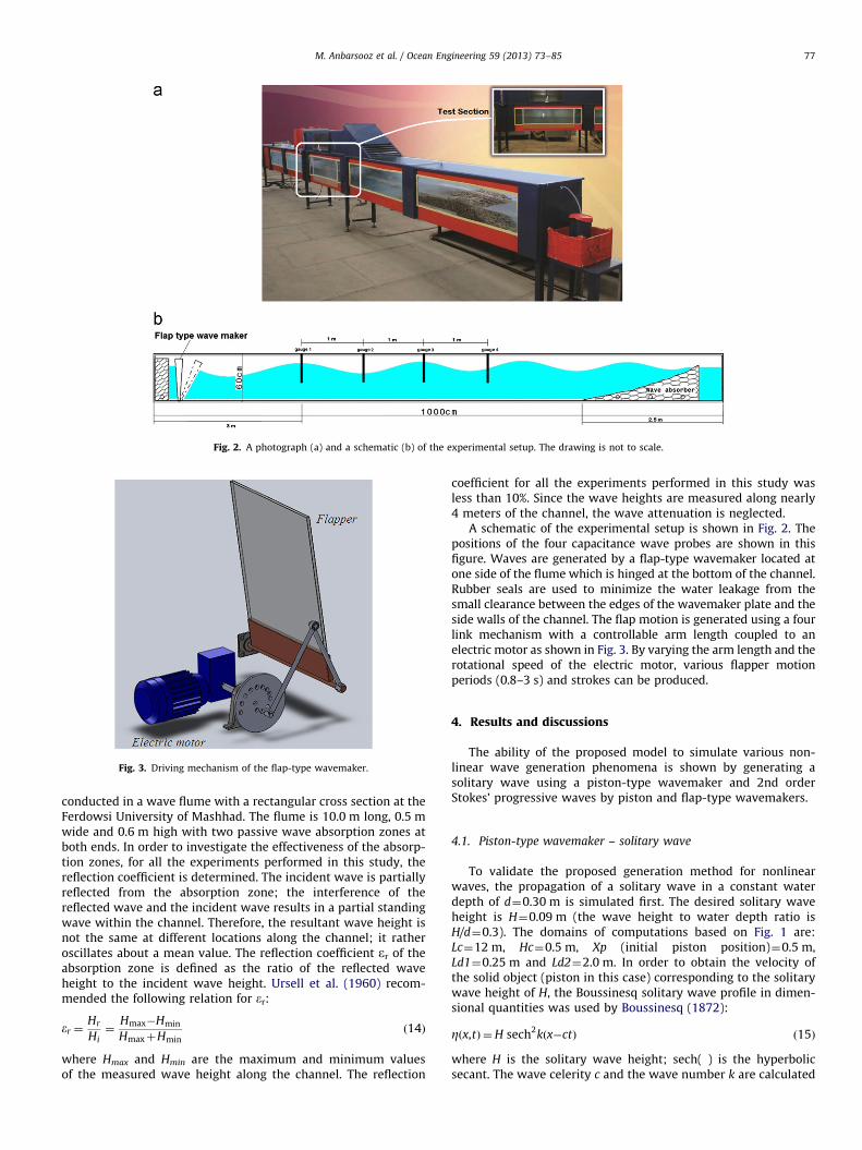
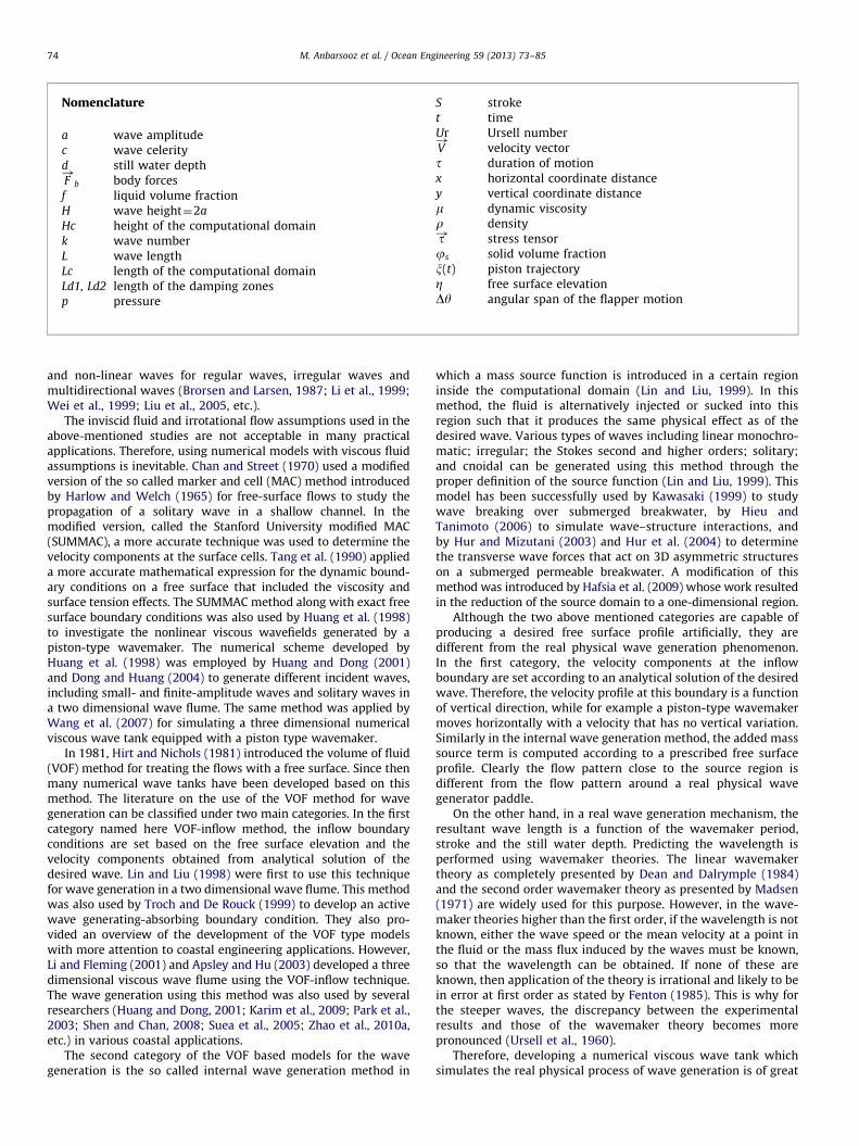
Fig. 2. A photograph (a) and a schematic (b) of the experimental setup. The drawing is not to scale.

Fig. 3. Driving mechanism of the flap-type wavemaker.

M. Anbarsooz et al. / Ocean Engineering 59 (2013) 73–85 77

conducted in a wave flume with a rectangular cross section at theFerdowsi University of Mashhad. The flume is 10.0 m long, 0.5 mwide and 0.6 m high with two passive wave absorption zones atboth ends. In order to investigate the effectiveness of the absorp-tion zones, for all the experiments performed in this study, thereflection coefficient is determined. The incident wave is partiallyreflected from the absorption zone; the interference of thereflected wave and the incident wave results in a partial standingwave within the channel. Therefore, the resultant wave height isnot the same at different locations along the channel; it ratheroscillates about a mean value. The reflection coefficient er of theabsorption zone is defined as the ratio of the reflected waveheight to the incident wave height. Ursell et al. (1960) recom-mended the following relation for er:

er ¼Hr

Hi¼

Hmax�Hmin

HmaxþHminð14Þ

where Hmax and Hmin are the maximum and minimum valuesof the measured wave height along the channel. The reflection

coefficient for all the experiments performed in this study wasless than 10%. Since the wave heights are measured along nearly4 meters of the channel, the wave attenuation is neglected.

A schematic of the experimental setup is shown in Fig. 2. Thepositions of the four capacitance wave probes are shown in thisfigure. Waves are generated by a flap-type wavemaker located atone side of the flume which is hinged at the bottom of the channel.Rubber seals are used to minimize the water leakage from thesmall clearance between the edges of the wavemaker plate and theside walls of the channel. The flap motion is generated using a fourlink mechanism with a controllable arm length coupled to anelectric motor as shown in Fig. 3. By varying the arm length and therotational speed of the electric motor, various flapper motionperiods (0.8–3 s) and strokes can be produced.

4. Results and discussions

The ability of the proposed model to simulate various non-linear wave generation phenomena is shown by generating asolitary wave using a piston-type wavemaker and 2nd orderStokes’ progressive waves by piston and flap-type wavemakers.

4.1. Piston-type wavemaker – solitary wave

To validate the proposed generation method for nonlinearwaves, the propagation of a solitary wave in a constant waterdepth of d¼0.30 m is simulated first. The desired solitary waveheight is H¼0.09 m (the wave height to water depth ratio isH/d¼0.3). The domains of computations based on Fig. 1 are:Lc¼12 m, Hc¼0.5 m, Xp (initial piston position)¼0.5 m,Ld1¼0.25 m and Ld2¼2.0 m. In order to obtain the velocity ofthe solid object (piston in this case) corresponding to the solitarywave height of H, the Boussinesq solitary wave profile in dimen-sional quantities was used by Boussinesq (1872):

Z x,tð Þ ¼H sech2k x�ctð Þ ð15Þ

where H is the solitary wave height; sech( ) is the hyperbolicsecant. The wave celerity c and the wave number k are calculated

5 10 15 20 25 30 35 40

0

0.3

0.6

Boussinesq,analyticalNumerical,CPD=24Numerical,CPD=36Numerical,CPD=48

η/d

M. Anbarsooz et al. / Ocean Engineering 59 (2013) 73–8578

as:

c¼ffiffiffiffiffiffiffiffiffiffiffiffiffiffiffiffiffig Hþdð Þ

pð16Þ

k¼

ffiffiffiffiffiffiffiffi3H

4d3

sð17Þ

Referring to the solitary wave generation theory developed byGoring (1979), the piston trajectory for generating the solitarywaves of all heights is:

xðtÞS¼ tanh7:6

t

t�1

2

� �ð18Þ

where S is the piston stroke and t is the duration of motioncalculated as:

S¼2H

kd¼

ffiffiffiffiffiffiffiffiffiffi16H

3d

rd ð19Þ

and

t¼ 2

kc3:80þ

H

d

� �ð20Þ

In the developed model in this study as described above, thevelocity of the solid object is set during the computations in eachtime step. Therefore, the velocity of the piston is calculated bytaking derivative of Eq. (18) with respect to time leading to:

VðtÞ

S¼

7:6

tsech27:6

t

t�

1

2

� �ð21Þ

When generating a solitary wave using a piston-type wavemaker,an oscillatory tail is always formed behind the wave. Goring(1979) reported the height of the oscillatory wave to be around25% of the main wave when using a linear trajectory for the pistonmovement. The height of the oscillatory wave, however, wasreduced to 10%of the main wave when the trajectory of the piston was set basedon Eq. (18).

The water free surface profile as the piston moves inside thefluid based on Eq. (18) is depicted in Fig. 4. The time duration andstroke of the piston motion are 3.35 s and 0.379 m, respectively.The generation of the solitary wave is completed in this time after

Fig. 4. Evolution of the numerical free surface profile for the solitary wave

(H/d¼0.3).

which the shape of the wave remains nearly unchanged. Thecomputational grid size was set based on a mesh refinementstudy in which the mesh size was progressively increased until nosignification changes were observed in the results. For the entirecases in this study, a uniform mesh was used; therefore, the meshsize was characterized by the number of grids used for a lengthscale considered to be the initial water depth in this case. Threedifferent mesh sizes corresponding to 24, 36 and 48 cells perdepth (CPD) in the still water were considered. The solitary waveprofiles generated using the three mesh sizes are compared withthat of the analytical solution in Fig. 5. A good agreement can beseen between the results of simulations and analytics. The figurealso illustrates that the results are independent of the mesh size;as a result, for most simulations in this study, a mesh size ofCPD¼24 was selected. The discrepancy observed between simu-lations and analytics at the tail of the solitary wave is due to theexistence of the oscillatory wave as described above. The height ofthis oscillatory wave is about 10% of that of the solitary wave. Itshould be mentioned that the same procedure taken to obtain theoptimum mesh size was also followed for the computational time

x/d

Fig. 5. Free surface profile compared to analytical results for various mesh sizes

characterized by CPD (cell-per-depth).

x/d10 20 30 40

-0.3

-0.2

-0.1

0

0.1

0.2

0.3

0.4

0.5

0.6

η/d

(a) (b) (c)

Fig. 6. Numerical free surface profiles at different times: (a) ta¼3.0 s; (b) tb¼4.0 s;

(c) tc¼5.0 s.

u and v (m/s)

y (m

m)

-0.2 0 0.2 0.4 0.6 0.80

50

100

150

200

250

300 u Numericalu Analyticalv Numericalv Analytical

u and v (m/s)

y (m

m)

0 0.20

50

100

150

200

250

300u Numericalu Analyticalv Numericalv Analytical

Fig. 7. Horizontal (u) and vertical (v) velocity profiles induced by a solitary wave of H/d¼0.3.

x[mm]

y[m

m]

4000 5000 6000 7000 8000 90000

50

100

150

200

250

300

350

400

450

500

1 m/s

x/L=0.0 x/L=0.2

Fig. 8. The solitary wave profile (H/d¼0.3) and the velocity field at t¼4.0 s.

M. Anbarsooz et al. / Ocean Engineering 59 (2013) 73–85 79

step after which a time step of 0.001 s was found to be theoptimum value.

The calculated shape of the solitary wave at progressive timesis plotted in Fig. 6. The oscillatory tail behind the wave can bewell observed in the figure. The wave propagates with a constantvelocity and a stable shape towards the end of the computationaldomain. This is seen in the figure by the equal distances traveledby the wave in the same time intervals.

The accuracy of the numerical results are also validated bycomparing the generated velocity field due to wave motion withthe analytical results of inviscid fluid (Dean and Dalrymple, 1984).The horizontal and vertical velocity components are plotted incomparison with those of the analytical in Fig. 7 at t¼4 s elapsedafter the start of the piston motion for the solitary wave ofH/d¼0.3. The vertical variation of the velocity components areshown at two positions; just under the wave crest (x/L¼0.0) andat 0.2L after the crest (x/L¼0.2) (the two positions are alsodisplayed in Fig. 8). A good agreement is seen between the tworesults; the small discrepancy that exists in the horizontalvelocity under the crest may be due to the error in the analytics.The order of accuracy of the analytical solution is O((H/d)2,

(H/d)(d/L)2) as presented in Dean and Dalrymple (1984). For thesolitary wave studied in this paper, H/d¼0.3 and d/L¼0.0756,therefore, the accuracy of the analytical solution is in the order of0.09. Thus, the discrepancy observed between the numericalresults and the analytical solution in Fig. 7 may be due to theerror in the analytics.

A better representation of the solitary wave profile and thecorresponding velocity field at t¼4 sec are shown in Fig. 8. It isobserved that the velocity before the wave crest is downwardwhile after the crest the fluid attains an upward velocity. How-ever, right under the crest the fluid has no vertical velocity.

4.2. Piston type wavemaker – progressive waves

To verify the accuracy of the numerical results in the case of apiston-type wavemaker, the results are compared with reportedexperiments, analytics and other numerical results. For thispurpose, the experimental measurements of Ursell et al. (1960),the second order wavemaker theory of Madsen (1971), and thenumerical results of Huang et al. (1998) are considered.

M. Anbarsooz et al. / Ocean Engineering 59 (2013) 73–8580

Ursell et al. (1960) performed experiments in a 100-ft-longchannel that had an inclined plate with a slope of 1:15 at the farend to absorb the wave energy. The effect of the wave reflectionwas also taken into account. They divided their experiments intotwo categories, namely, small wave steepness (0.002rH/Lr0.03)and large wave steepness (0.045rH/Lr0.048). Most of theexperiments (20 cases) were classified as small wave steepness;while the cases with large wave steepness were limited to fourcases. Huang et al. (1998) recalculated seven of the 24 experi-mental cases of Ursell et al. (1960) using their numerical model.In this paper, nine cases including all the four cases of Ursell et al.(1960) with large wave steepness are simulated. A typical casewith a higher wave steepness (H/L¼0.06) is also studied. Theexperimental conditions corresponding to these cases are shownin Table 1.

In all the numerical simulations, the piston is initially locatedat Xp¼0.5 m (Fig. 1a). The piston is placed inside the fluid domainto better visualize the capability of the model to capture the freesurface variation as the solid body movies inside the fluid. Thedomains of computations based on

Fig. 1 are considered as: Lc48L, Hc41.5d, Ld1¼0.25 m andLd242L. The mesh size considered in this case had 36 cells in thewater depth (i.e. CPD¼36). Also a time step of T/100 (where T isthe wave period) is found to be sufficiently small such that theresults are independent of time step.

Table 1Piston type wavemaker conditions; nMeasured values from Ursell et al. (1960).

Case number Period (s) Stroke (cm) Still water

depth (m)

(H/S)theor (H/S)measn

High wave steepness1 0.79 2.54 0.6096 1.99 1.88

2 0.85 3.15 0.4572 1.85 1.67

3 0.95 4.50 0.3048 1.39 1.22

4 0.96 5.73 0.2012 1.05 0.90

5 1.00 6.40 0.3000 1.30 –

Small wave steepness6 0.92 1.51 0.7315 1.97 1.90

7 1.11 1.56 0.7315 1.82 1.77

8 1.27 1.88 0.5090 1.32 1.20

9 2.09 2.06 0.4785 0.70 0.68

H/S

0 1 2 3 4 5 60

0.5

1

1.5

2

2.5

3 Wavemaker theoryExperiments of Ursell et al.Numerical results of Huang et al.Present numerical method

2πd/L

Fig. 9. Comparison between the solution of the wavemaker theory, experiments of Urs

of the present study.

The numerical results for the aforementioned experimentalconditions are shown in Fig. 9 in comparison with the experi-mental and analytical results. To obtain the values of the waveprofile from numerical calculations, a section close to the middleof the channel away from the piston and the damping zone at theend of the channel is considered. This section was selectedbetween two positions distanced 5d and 25d away from thepiston location. Specifically, the numerical wave height is calcu-lated by averaging the wave heights from the free surface timehistory at a fixed position with a distance equal to 15d away fromthe wavemaker initial position. However, the wavelength iscalculated by averaging the wave lengths taken from the freesurface space distribution inside the selected section.

The numerical results from the present study for both smalland large wave steepness are compared with those of the Ursellet al. (1960) experiments and Huang et al. (1998) numericalcalculations in Fig. 9. The results from the wavemaker theory arealso displayed in the figure. As observed in the figure, thenumerical results from the present model agree well with thoseof the experiments for both small and large wave steepness.Compared to the analytical results, however, it is seen that bothnumerical simulations and experiments indicate a better agree-ment in small wave steepness. The time evolution of the numer-ical free surface profile as the piston starts its motion inside thewater for a case with maximum wave steepness (the Case #5 of

(H/S)num (2pd/L)theor (2pd/L)num (H/L)theory Experiment number in

Ursell et al. (1960)

1.86 3.98 3.85 0.0488 21

1.65 2.55 2.43 0.0485 22

1.24 1.51 1.45 0.0439 23

0.92 1.09 1.04 0.0409 24

1.10 1.37 1.30 0.0602 –

1.98 3.52 3.28 0.0230 9

1.70 2.44 2.36 0.0153 13

1.28 1.42 1.39 0.0094 17

0.73 0.72 0.70 0.0096 15

2πd/L

H/S

0 1 2 3 4 5 60

0.5

1

1.5

2

2.5

3 Wavemaker theoryExperiments of Ursell et al.Numerical results of Huang et al.Present numerical method

ell et al. (1960), numerical results of Huang et al. (1998) and the numerical results

Fig. 10. Evolution of the numerical free surface profile for the piston type wavemaker.

t/T0 2 4 6 8

-0.1

-0.05

0

0.05

0.1 AnalyticalNumerical

(m)

η

Fig. 11. Comparison between the numerical and analytical free surface elevation

at x¼5 m.

x(m)4 5 6 7

-0.1

-0.05

0

0.05

0.1AnalyticalNumerical

(m)

η

Fig. 12. Comparison between the numerical and analytical wave profile at t/T¼10.

M. Anbarsooz et al. / Ocean Engineering 59 (2013) 73–85 81

Table 1) is shown in Fig. 10. It is seen that after nearly 10T thewave profile reaches a steady state shape. It should be mentionedthat the piston stroke for this case is 6.4 cm (see Table 1) which istoo small compared to the channel length (12 m); as a result, thepiston displacement cannot be recognized in the figure. Fig. 11shows time evolution of the numerical water free surface eleva-tion (measured from the still water height) at 15 water depthsaway from the wavemaker in comparison with the analyticalresults. After nearly four periods, the wave approaches its steady

profile. The numerical and analytical results are also comparedwith each other at the dimensionless time of t/T¼10.0 in Fig. 12.The wave profiles from the two results almost coincide in phasebut the analytical wave heights are slightly larger than those ofthe simulations.

4.3. Flap type wavemaker – progressive waves

In the case of flap type wavemaker, the numerical results arecompared with the measurements performed in this study asdescribed in Section 3, analytical results as presented in Dean and

Table 2Flap type wavemaker conditions. nMeasured values from the current study.

Case number Period (sec) Stroke (cm) Still water depth (m) (H/S)theor (H/S)num (H/S)measn (2pd/L)theor (2pd/L)num (H/L)theor

Small wave steepness

1 2.1 8.45 0.30 0.28 0.27 0.32 0.548 0.531 0.0069

2 1.40 8.45 0.30 0.46 0.47 0.47 0.875 0.877 0.0180

3 1.05 3.15 0.45 0.93 0.92 — 1.747 1.756 0.0181

4 1.05 2.40 0.8 1.34 1.25 — 2.941 2.717 0.0188

5 1.00 3.00 1.0 1.51 1.40 — 4.030 4.189 0.0291

6 1.40 8.57 0.50 0.65 0.62 0.63 1.222 1.208 0.0217

High wave steepness7 0.84 8.47 0.40 1.17 0.96 0.99 2.330 2.244 0.0919

8 1.05 8.45 0.30 0.68 0.65 0.63 1.279 1.160 0.0389

9 0.84 8.45 0.30 0.96 0.76 0.80 1.808 1.804 0.0778

10 1.05 6.30 0.90 1.41 1.25 — 3.299 3.250 0.0518

11 1.05 8.40 1.20 1.55 1.31 — 4.384 4.076 0.0757

12 1.05 4.69 0.67 1.22 1.09 — 2.485 2.392 0.0337

Fig. 13. Evolution of the numerical free surface profile for the flap type wavemaker.

M. Anbarsooz et al. / Ocean Engineering 59 (2013) 73–8582

Dalrymple (1984) and the numerical results of the Finnegan andGoggins (2012). Twelve cases are studied in this section, whichare again classified as small and large wave steepness includingintermediate and deep water, as tabulated in Table 2. However,the experimental results of the present study are limited tointermediate water depths (p/10rkdrp). As a result, for the

deep water cases, the numerical results are only compared withthe analytical results of the wavemaker theory (Dean andDalrymple, 1984).

In the numerical simulations, the solid body representing theflapper is initially located at Xp¼0.5 m (Fig. 1b). The solid bodyhas no translational velocity, but a simple harmonic angular

M. Anbarsooz et al. / Ocean Engineering 59 (2013) 73–85 83

velocity as:

y tð Þ ¼Dy2

cos2pT

t

� �ð22Þ

where Dy is the angular span of the flapper motion. The stroke ofthe flapper depends on both the angular span and the still waterdepth as:

S¼ 2d� tanDy2

� �ð23Þ

For the cases with a high wave steepness and for the deep watercases, the motion of the flapper is initiated using a linear timeramp according to Zhao et al. (2010b). A duration of 2T for thetime ramp was enough to eliminate the initial instabilities.

The time evolution of the numerical free surface profile as theflap starts its motion inside the water for a typical case withrelatively large wave steepness (the Case #9 of Table 2) is shownin Fig. 13. The duration of the time ramp used in this case was 2T.The rotation of the flap and the consequent formation of theprogressive waves can be well observed in this figure. Thenumerical wave heights for all the cases listed in Table 2 arecalculated as described for the piston wavemaker, in Section 4.2.The comparison between the numerical results, the wavemakertheory and the experimental data is presented in Fig. 14. In thefigure, the ranges of shallow, intermediate and deep water arespecified based on the classifications presented by Dean andDalrymple (1984). For the waves with a small steepness, a goodagreement between the numerical and experimental results canbe observed especially at intermediate water depths (seeFig. 14a). As observed in the figure, the numerical model of

2πd/L

H/S

0 2 4 60

0.5

1

1.5

Wavemaker theoryNumerical results of Finnegan et al.Numerical results of the present studyMeasurments of the present study

intermediate water deep water

shal

low

wat

er

Fig. 14. Comparison between the solution of the wavemaker theory, numerical resu

of the present study.

Table 3Inputs required for the two mavemakers, generating a wave with c

Desired wave characterestics

Height (cm) Normalized wave number

2.84 2.44

Input required for piston-type wavemaker motion

Stroke (cm) Period (s)

1.56 1.11

Finnegan and Goggins (2012) fails at deep water waves for aflap-type wavemaker hinged at the bottom of the flume. Theyfound that wave generation in the ANSYS CFX using a flap-typewavemaker is restricted to a low normalized wave number, kd. Inorder to increase this restriction, the hinge of the wavemaker wasraised and, with this alteration, it was possible to generate deepwater linear waves. This is while the results of the present modeldo not reveal such a limitation. As seen in Fig. 14a, the modelpresented in this paper can predict deep water waves with anacceptable accuracy (less than 5%). However, for the cases with alarge wave steepness (Fig. 14b) both the numerical and experi-mental results are about 10% below those of the wavemakertheory; this finding is the same as was observed for the pistontype wavemaker (Section 4.2).

The discrepancy between the experiments and the wavemakertheory for the cases with large wave steepness may be attributed tothe error in calculating the wave length in the theory. In thewavemaker theory, the wavelength is calculated using the well-known dispersion relation, s2

¼gk tanh kdþO(ka)2 (Whitham,1974). This relation shows that as the wave steepness (ka/p)increases, the error in calculating the wave length increases.However, using the proposed method in this paper, one only needsto specify the period and stroke of the wavemaker’s trajectory in awater of specific depth. The wave length and the wave height willbe calculated through the complete solution of the Navier-Stokesequations. Therefore, the results of the proposed numerical methodshow a better agreement with the experimental data especially forthe waves with high wave steepness.

In order to generate a desired wave, one may use either a piston-type or a flap-type wavemaker by appropriately adjusting the

2πd/L

H/S

0 2 4 60

0.5

1

1.5

Wavemaker theoryNumerical results of the present studyMeasurments of the present study

deep waterintermediate water

shal

low

wat

er

lts of Finnegan and Goggins (2012) and the numerical and experimental results

haracteristics of Case #7 of Table 1.

Water depth (m) Period (s)

0.7315 1.11

Input required for flap-type wavemaker motion

Stroke (cm) Period (s)

1.20 1.11

y coordinate (mm)

u (m

/s)

0 100 200 300 400 500 600 700-0.1

-0.05

0

0.05

0.1

0.15 AnalyticalPiston-typeFlap-type

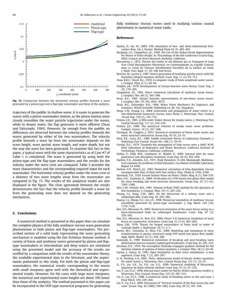
Fig. 15. Comparison between the horizontal velocity profiles beneath a wave

generated by a piston-type and a flap-type wavemaker and those of the analytics.

M. Anbarsooz et al. / Ocean Engineering 59 (2013) 73–8584

trajectory of the paddle. In shallow water, it is easier to generate thewaves with a piston wavemaker motion, as the piston motion moreclosely resembles the water particle trajectories under the waves,while in deeper water, the flap generator is more efficient (Deanand Dalrymple, 1984). However, far enough from the paddle, nodifferences are observed between the velocity profiles beneath thewaves generated by either of the two wavemakers. The velocityprofile beneath a wave far from the wavemaker depends on thewave height, wave period, wave length, and water depth, but notthe way the wave has been generated. To examine this fact in thispaper, a typical wave with the same characteristics as of Case #7 ofTable 1 is considered. The wave is generated by using both thepiston-type and the flap-type wavemakers and the results for thevelocity under the wave crest are compared. Table 3 provides thewave characteristics and the corresponding required input for eachwavemaker. The horizontal velocity profiles under the wave crest ata distance of two wave lengths away from the wavemaker arecompared in Fig. 15. The results of the analytical model are alsodisplayed in the figure. The close agreement between the resultsdemonstrates the fact that the velocity profile beneath a wave farfrom the generating zone does not depend on the generatingmechanism.

5. Conclusions

A numerical method is presented in this paper that can simulatethe complete physics of the fully nonlinear viscous wave generationphenomenon in both piston and flap-type wavemakers. The pre-scribed motion of a solid body representing the wave generatingmechanism is modeled using the fast fictitious domain method. Avariety of linear and nonlinear waves generated by piston and flap-type wavemakers in intermediate and deep waters are simulatedusing the presented model and the accuracy of the results areverified by a comparison with the results of the wavemaker theory,the available experimental data in the literature, and the experi-ments preformed in this study. For both the piston and flap-typewavemakers, the numerical results corresponding to the waveswith small steepness agree well with the theoretical and experi-mental results. However, for the cases with large wave steepness,the numerical and experimental wave heights are about 10% lowerthan those of the analytics. The method presented in this paper canbe incorporated in the VOF-type numerical programs for generating

fully nonlinear viscous waves used in studying various coastalphenomena in numerical wave tanks.

References

Apsley, D., Hu, W., 2003. CFD simulation of two- and three-dimensional free-surface flow. Int. J. Numer. Method Fluid 42 (5), 465–491.

Borgman, L.E., Chappelear, J.E., 1958. The Use of the Stokes-Struik Approximationfor Waves of Finite Height. In: Proceedings of the 6th Conference Coastal Eng.,ASCE, Council on Wave Research, Berkeley, California.

Boussinesq, J., 1872. Theorie des Ondes et des Remous qui se Propagent le Longd’un Canal Rectangulaire Horizontal, en Communiquant au Liquide Contenudans ce Canal de Vitesses Sensiblement Parreilles de la Surface au Fond.J. Math. Pure Appl. 17, 55–108 2nd Series.

Brorsen, M., Larsen, J., 1987. Source generation of nonlinear gravity waves with theboundary integral equation method. Coast. Eng. 11 (2), 93–113.

Chan, R.K.C., Street, R.L., 1970. A computer study of finite-amplitude water waves.J. Comput. Phys. 6 (1), 68–94.

Chaplin, J.R., 1979. Developments of stream-function wave theory. Coast. Eng. 3(0), 179–205.

Chappelear, J.E., 1961. Direct numerical calculation of nonlinear ocean waves.J. Geophys. Res. 66 (2), 501–508.

Dean, R.G., 1965. Stream function representation of non-linear ocean waves.J. Geophys. Res. 70 (18), 4561–4572.

Dean, R.G., Dalrymple, R.A., 1984. Water Wave Mechanics for Engineers andScientists. World Scientific Publishing Co. Re. ttd., Singapore.

Dong, C.M., Huang, C.J., 2004. Generation and propagation of water waves in atwo-dimensional numerical viscous wave flume. J. Waterway, Port, Coastal,.Ocean Eng. 130 (3), 143–153.

Fenton, J.D., 1985. A fifth-order Stokes theory for steady waves. J. Waterway PortCoastal Ocean Eng. 111 (2), 216–234.

Fenton, J.D., 1988. The numerical solution of steady water wave problems.Comput. Geosci. 14 (3), 357–368.

Finnegan, W., Goggins, J., 2012. Numerical simulation of linear water waves andwave–structure interaction. Ocean Eng. 43 (0), 23–31.

Flick, R.E., Guza, R.T., 1980. Paddle Generated Waves in Laboratory Channels. J.Waterway Port Coastal .Ocean Div. 106 (1), 79–97.

Goring, D.G., 1979. Tsunamis-the propagation of long waves onto a shelf, W.M.Keck Laboratory of Hydraulics and Water Resources, California Institute ofTechnology, Pasadena, California, California.

Hafsia, Z., Hadj, M.B., Lamloumi, H., Maalel, K., 2009. Internal inlet for wavegeneration and absorption treatment. Coast Eng. 56 (9), 951–959.

Harlow, F.H., Amsden, A.A., 1971. Fluid Dynamics: A LASL Monograph, Mathema-tical solutions for problems in fluid dynamics. Los Alamos Scientific LaboratoryReport LA 4700.

Harlow, F.H., Welch, J.E., 1965. Numerical calculation of time-dependent viscousincompressible flow of fluid with free surface. Phys. Fluids 8, 2182–2189.

Havelock, T.H., 1929. Forced Surface Wave on Water. Philos. Mag. 8 (7), 569–576.Hieu, P.D., Tanimoto, K., 2006. Verification of a VOF-based two-phase flow model

for wave breaking and wave-structure interactions. Ocean Eng. 33 (11–12),1565–1588.

Hirt, C.W., Nichols, B.D., 1981. Volume of fluid (VOF) method for the dynamics offree boundaries. J. Comput. Phys. 39 (1), 201–225.

Huang, C.J., Dong, C.M., 2001. On the interaction of a solitary wave and asubmerged dike. Coast Eng. 43, 265–286.

Huang, C.J., Zhang, E.C., Lee, J.F., 1998. Numerical simulation of nonlinear viscouswavefields generated by piston-type wavemaker. J. Eng. Mech. 124 (10),1110–1120.

Hur, D.S., Mizutani, N., 2003. Numerical estimation of the wave forces acting on athree-dimensional body on submerged breakwater. Coast. Eng. 47 (3),329–345.

Hur, D.S., Mizutani, N., Kim, D.S., 2004. Direct 3-D numerical simulation of waveforces on asymmetric structures. Coast Eng. 51 (5–6), 407–420.

Hyun, J.M., 1976. Theory for hinged wavemakers of finite draft in water ofconstant depth. J. Hydronaut. 10 (1), 2–7.

Karim, M.F., Tanimoto, K., Hieu, P.D., 2009. Modelling and simulation of wavetransformation in porous structures using VOF based two-phase flow model.Appl. Math. Model. 33 (1), 343–360.

Kawasaki, K., 1999. Numerical simulation of breaking and post-breaking wavedeformation process around a submerged breakwater. Coast Eng. 41, 201–223.

Kershaw, D.S., 1978. The incomplete Cholesky-conjugate gradient method for theiterative solution of systems of linear equations. J. Comput. Phys. 26 (1), 43–65.

Larsen, J., Dancy, H., 1983. Open boundaries in short wave simulations—a newapproach. Coast Eng. 7 (3), 285–297.

Li, B., Fleming, C.A., 2001. Three -dimensional model of Navier–Stokes equationsfor water waves. J. Waterway, Port, Coastal Ocean Eng. 127 (1), 16–25.

Li, Y.S., Liu, S.X., Yu, Y.X., Lai, G.Z., 1999. Numerical modeling of Boussinesqequations by finite element method. Coast Eng. 37 (2), 97–122.

Lin, P., Liu, P.L.F., 1999. Internal wave-maker for Navier-Stokes equations models. J.Waterway, Port, Coastal, Ocean Eng. 125 (4), 207–215.

Lin, P., Liu, P.L.F., 1998. A numerical study of breaking waves in the surf zone. JFluid Mech. 359, 239–264.

Lin, P., Liu, P.L.F., 2004. Discussion of ‘‘Vertical variation of the flow across the surfzone’’ [Coast. Eng. 45 (2002) 169–198]. Coast Eng. 50 (3), 161–164.

M. Anbarsooz et al. / Ocean Engineering 59 (2013) 73–85 85

Liu, S.X., Teng, B., Yu, Y.X., 2005. Wave generation in a computation domain. Appl.Math. Model. 29 (1), 1–17.

Madsen, O.S., 1971. On the Generation of Long Waves. J. Geophys. Res. 76,8672–8683.

Mirzaii, I., Passandideh-Fard, M., 2012. Modeling free surface flows in presence ofan arbitrary moving object. Int. J. Multiphase Flow 39 (0), 216–226.

Moubayed, W., Williams, A., 1993. Second-order bichroamatic waves produced bya generic planar wavemaker in a two-dimensional flume. J. Fluid Struct. 8(73–92), 73.

Park, J.C., Kim, M.H., Miyata, H., Chun, H.H., 2003. Fully nonlinear numerical wavetank (NWT) simulations and wave run-up prediction around 3-D structures.Ocean Eng. 30 (15), 1969–1996.

Schaffer, H.A., 1996. Second-order wavemaker theory for irregular waves. OceanEng. 23 (1), 47–88.

Schwartz, L.W., 1974. Computer extension and analytic continuation of Stokes’expansion for gravity waves. J. Fluid Mech. 62 (03), 553–578.

Sharma, N., Patankar, N.A., 2005. A fast computation technique for the directnumerical simulation of rigid particulate flows. J. Comput. Phys. 205, 439–457.

Shen, L., Chan, E.-S., 2008. Numerical simulation of fluid–structure interactionusing a combined volume of fluid and immersed boundary method. OceanEng. 35 (8-9), 939–952.

Suea, Y.C., Chernb, M.J., Hwanga, R.R., 2005. Interaction of nonlinear progressiveviscous waves with a submerged obstacle. Ocean Eng. 32, 893–923.

Tang, C.T., Patel, V.C., Landweber, L., 1990. Viscous effects on propagation andreflection of solitary waves in shallow channels. J. Comput. Phys. 88 (1),86–113.

Troch, P., De Rouck, J., 1999. An active wave generating-absorbing boundarycondition for VOF type numerical model. Coast Eng. 38 (4), 223–247.

Ursell, F., Dean, R.G., Yu, Y.S., 1960. Forced small-amplitude water waves:A comparison of theory and experiment. J. Fluid Mech. 7, 32–53.

Wang, H.W., Huang, C.J., Wu, J., 2007. Simulation of a 3D Numerical Viscous WaveTank. J. Eng. Mech. 133 (7), 761–772.

Wei, G., Kirby, J.T., Sinha, A., 1999. Generation of waves in Boussinesq modelsusing a source function method. Coast Eng. 36 (4), 271–299.

Whitham, G.B., 1974. Linear and Nonlinear Waves. Wiley, New York.Wood, D.J., Pedersen, G.K., Jensen, A., 2003. Modelling of run up of steep non-

breaking waves. Ocean Eng. 30 (5), 625–644.Youngs, D.L., 1984. An interface tracking method for a 3D Eulerian hydrodynamics

code. Technical Report 44/92/35, AWRE.Zhang, H., Schaffer, H.A., 2007. Approximate stream function wavemaker theory

for highly non-linear waves in wave flumes. Ocean Eng. 34 (8-9), 1290–1302.Zhao, X.Z., Hu, C.H., Sun, Z.C., 2010a. Numerical simulation of extreme wave

generation using VOF method. J. Hydrodyn. Ser. B 22 (4), 466–477.Zhao, X.Z., Hu, C.H., Sun, Z.C., Liang, S.X., 2010b. Validation of the initialization of a

numerical wave flume using a time ramp. Fluid Dyn. Res. 42, 045504.