Full waveform seismic inversion using a distributed system ... · seismic inversion of a large...

CONCURRENCY AND COMPUTATION: PRACTICE AND EXPERIENCEConcurrency Computat.: Pract. Exper. 2005; 17:1365–1385Published online in Wiley InterScience (www.interscience.wiley.com). DOI: 10.1002/cpe.897

Full waveform seismic inversionusing a distributed systemof computers

Indrajit G. Roy1, Mrinal K. Sen1,∗,† andCarlos Torres-Verdin2

1Institute for Geophysics, John A. and Katherine G. Jackson School of Geosciences,The University of Texas at Austin, Austin, TX 78759, U.S.A.2Department of Petroleum and Geo-systems Engineering, The University of Texas at Austin, Austin,TX 78759, U.S.A.

SUMMARY

The aim of seismic waveform inversion is to estimate the elastic properties of the Earth’s subsurface layersfrom recordings of seismic waveform data. This is usually accomplished by using constrained optimizationoften based on very simplistic assumptions. Full waveform inversion uses a more accurate wave propagationmodel but is extremely difficult to use for routine analysis and interpretation. This is because computationaldifficulties arise due to: (1) strong nonlinearity of the inverse problem; (2) extreme ill-posedness; and(3) large dimensions of data and model spaces. We show that some of these difficulties can be overcomeby using: (1) an improved forward problem solver and efficient technique to generate sensitivity matrix;(2) an iteration adaptive regularized truncated Gauss–Newton technique; (3) an efficient technique formatrix–matrix and matrix–vector multiplication; and (4) a parallel programming implementation witha distributed system of processors. We use a message-passing interface in the parallel programmingenvironment. We present inversion results for synthetic and field data, and a performance analysis of ourparallel implementation. Copyright c© 2005 John Wiley & Sons, Ltd.

KEY WORDS: seismic waveform; inversion; adaptive regularization; distributed systems

1. INTRODUCTION

Full waveform inversion of seismic data in a pre-stack domain is important for delineating detailedmaps of elastic properties, e.g. bulk and shear moduli and density, of hydrocarbon reservoirs that aid in

∗Correspondence to: Mrinal K. Sen, Institute for Geophysics, John A. and Katherine G. Jackson School of Geosciences,The University of Texas at Austin, Austin, TX 78759, U.S.A.†E-mail: [email protected]

Contract/grant sponsor: U.S. Department of Energy; contract/grant number: #DE-FC26-00BC15305

Copyright c© 2005 John Wiley & Sons, Ltd.Received 1 May 2003

Revised 5 December 2003Accepted 26 February 2004

1366 I. G. ROY, M. K. SEN AND C. TORRES-VERDIN

fluid flow modeling and in the characterization of a hydrocarbon producing reservoir. The seismicmeasurements or data are the digitized version of the measured wave field generated due to anexplosive source, which propagates through the subsurface and returns to the receiving instrumentsafter reflection, refraction, diffraction and scattering from a medium with varying elastic propertiesand density. The wave field is measured in spatially distributed receivers, where each receiver records aseismogram (e.g. ground displacements or pressure variation as a function of time, often called traces).All such seismograms may be distributed into subgroups such that all of the elements in each subgroupshare the same property (usually geometrical distribution or layout). In a pre-stack full waveformseismic inversion, we deal with one such group of seismic traces. Note that each measured seismictrace is the digitized time series with equal sampling interval. Each seismic trace in a group is definedwith a unique value of source–receiver distance, known as the offset value. Therefore, the ensemble ofthe traces in a group is defined in the offset-time domain.

At the outset we define two important terminologies: inverse and forward problems. The simplestand the most successful approach to inversion is based on model-based data fitting in which a set ofobserved data is compared with the numerically computed data corresponding to some feasible Earthmodel using some measure of misfit or norm. If the misfit is not acceptable, the model is perturbed; dataare regenerated and compared with the observations until an acceptable model is found. Thus inversionis the process of deriving Earth models from observations. On the other hand, by forward modeling,we mean the computational scheme to generate a set of data or observations, given a model and aphysical theory. A forward problem solver is thus one of the important computational componentsof a model-based inversion in which a new model is generated recursively and the forward problemsolver is executed in every step of recursion until the acceptance criterion is reached. The complexity ofthe model and its parameterization often make the forward problem solver computationally intensive,resulting in computer-intensive inverse problems. Since we are interested in delineating the variationof elastic properties of the subsurface in detail, the model parameter space can also be very large(depending upon the parameterization scheme). Therefore, the practical application of a full waveformseismic inversion of a large volume of data in the pre-stack domain remains one of the outstandingchallenges in exploration seismics. The difficulties encountered in pre-stack waveform inversion areoutlined below:

• full waveform seismic inverse problem is extremely nonlinear;• inverse problem is ill-posed;• large dimensions of data and model could generate the curse of dimensionality;• non-uniqueness of the inverse problem.

These difficulties are intrinsic to many inverse problems in science and engineering and need specialattention. The large dimensionality of data and model spaces and the computationally intensive forwardmodeling procedure makes seismic waveform inversion impractical for any routine use. However,with the recent technological advancements in low-cost high-speed computational facilities, it is notunrealistic to hope to develop a robust and efficient pre-stack inversion algorithm for application to thethree-dimensional volume of a seismic data set using a cluster of PCs in a high-speed network with anefficient paradigm of parallelization of computational tasks.

To this end, we have designed and implemented a parallel version of a full waveform pre-stackseismic inversion algorithm on a homogeneous cluster of distributed memory parallel computer(DMPC) environment. Producing a parallel implementation of the inversion algorithm is generally

Copyright c© 2005 John Wiley & Sons, Ltd. Concurrency Computat.: Pract. Exper. 2005; 17:1365–1385

FULL WAVEFORM SEISMIC INVERSION USING A DISTRIBUTED SYSTEM OF COMPUTERS 1367

more complex than producing an equivalent sequential implementation. Nevertheless, implementationof a parallel programming paradigm is being increasingly used in seismic data processing, especially intime/depth migration (e.g. [1–3]), spectral analysis of the seismic trace [4], seismic wave propagationin elastic media [5] and acoustic inversion [6]. In this paper, we demonstrate the achievable practicalityin inverting a pre-stack two-dimensional set of seismic data using an efficient gradient-based iterativealgorithm and parallel computing with distributed systems connected by a high-speed network.Although we have applied our inversion algorithm to two-dimensional seismic data sets, our inversionalgorithm is valid for locally one-dimensional model in which we have assumed that Earth’s propertyvaries with depth only. In realizing pre-stack inversion on an entire two-dimensional seismic data set,we implement our inversion algorithm sequentially in every surface located Grid point.

To make the inversion algorithm robust and efficient we consider the following improvements in ouralgorithm:

• formulation of inversion in the plane-wave domain;• efficient forward modeling and sensitivity matrix computation;• design of truncated regularized Gauss–Newton (RGN) optimization algorithm;• selection of an iteration adaptive regularization parameter;• implementation of loop-level parallelization of the inversion algorithm using distributed systems

in a cluster.

Since we have designed our inversion algorithm in the plane-wave domain, we transform theensemble defined in the offset-time (x − t) domain to the slowness-intercept time (τ −p) domain usinga radon transform and scale the seismic traces appropriately. Inversion of plane-wave decomposedreflection seismic data was used earlier [7,8]. The rationale in considering plane-wave decomposeddata is to achieve rapid computational ability in the forward problem solver. We formalize our inversionalgorithm in a least squares sense and use a gradient-based optimization. To improve robustness andstability in computation, we improvise our gradient-based optimization scheme in the light of iteration-adaptive regularization.

2. THEORETICAL BACKGROUND

2.1. Forward problem solver and sensitivity matrix

We consider seismic wave propagation in a one-dimensional Earth where physical parameters(elastic moduli and density) vary vertically below the receiver position. We further consider thatthe inhomogeneous medium in which the seismic wave propagates is composed of a stack ofhomogeneous and isotropic layers having distinct values of the Earth model parameters. The seismicwave propagation in such a medium is characterized with a system of ordinary differential equations(ODEs). The theoretical background in developing a system of ODEs for seismic wave propagationin one-dimensional media is well established (see [9,10]). We start with the linearized momentumequation in the frequency domain given by

−ρω2u = ∇ · τ + f (1)

and the constitutive relation is given byτ = C : ε (2)



Region 1

A

B

Region 2

C

Region 1

A

B

Region 2

Region 1

A

B

Region 2

Region 1

A

B

Region 2

C

Figure 1. Schematic pole of the recursive scheme used to compare the response of the region AC. Each regionconsists of a stack of layers with varying values of elastic properties.

where, τ and ε are the infinitesimal stress and strain tensors, ρ is the density, u is the elasticdisplacement vector, f is the body force and C is a fourth-order elastic tensor. From the above twoequations, using Fourier–Hankel transform we can immediately derive the following system of ODEsas

∂zb = −iωAb + f (3)

where b = [ux uy uz τxz τyz τzz]T is called the stress-displacement vector whose elementsare displacements and tractions. The matrix A(ω, p) is called the system matrix, which is a functionof elastic coefficients and f is a body force term. Out of various techniques for solving (3), themethod of invariant imbedding or the reflection matrix [10], popularly known as the reflectivitymethod, is considered in our forward problem computation. The eigenvalues and eigenvectors of thematrix A are used to define four up-going and down-going reflection and transmission coefficientmatrices RD, TD, RU and TU. Those coefficients are propagated through the stack of layers to obtaina composite reflection matrix that includes the effects of reflection, transmission, mode conversion,internal multiples, etc.

Kennett [10] proposed that if the reflection and transmission matrices for two adjacent stack oflayers, say AB and BC (Figure 1) are known, then reflection/transmission matrices for a composite



layer AC can be obtained through the recursion relation given by

RACD = RAB

D + TABU RBC

D [I − RBCD ]−1TAB

D

TACD = TBC

D [I − RABU RBC

D ]−1TABD

RACU = RBC

U + TBCD RAB

U [I − RBCD RAB

U ]−1TBCU

TACU = TAB

U [I − RBCD RAB

U ]−1TBCU

(4)

The above recursion can be continued through the entire stack of layers by adding one new layerat a time. After computing reflection/transmission matrices through invariant imbedding we obtainsynthetic seismograms in the frequency-ray parameter domain. An inverse temporal Fourier transformgives the plane wave synthetics.

The generation of a sensitivity matrix is an essential element for any gradient-based optimizationmethod. Since model and data spaces for full waveform pre-stack inversion are very large, anefficient computational scheme is required for the generation of such matrices. A conventional bruteforce perturbation technique with finite difference is not considered, as it is very inefficient dueto a large number of calls to the forward problem solver corresponding to each model parameter.Randall [11] proposed a variant of the perturbation technique in which synthetic seismograms dueto perturbations in layer parameters are computed by combining partial upward and downwardreflection/transmission matrices. Such a technique enhances the efficiency of generation of thesensitivity matrix. Here we employed an approach developed in [12] that is more efficient than theapproach considered in [11], in which we avoid two steps of upward and downward propagationand simply evaluate new seismograms by reusing pre-computed reflectivity matrices from eitherupward or downward propagation alone. In a forward problem computation, we compute all fourreflection/transmission coefficient matrices for each layer in a top-down fashion and use the recursiveequations (4) to compute the above matrices for composite media. As we proceed in a top-downfashion, we store the composite response up to the current layer as a new layer is introduced intothe stack. We observe that a change in any one of the layer parameters corresponding to one layer ofthe model only affects reflection/transmission through itself and through layers that are immediatelyabove and below the current layers. Hence, for derivative calculation we take the following steps:

• perturb the parameters for one layer and compute reflection/transmission matrices for itself andthe layers above and below it;

• use the recursion relation to compute reflection/transmission matrices from the top layer all theway to the zone right above the perturbed layer;

• combine these with the reflection/transmission matrices of all the layers below it to computecomplete response.

The details of the algorithm for the computation of sensitivity matrix are outlined in [12].

2.2. Regularized least squares optimization

The pre-stack full waveform data set contain an ensemble of seismograms defined in τ − p (intercepttime-ray parameter) domain. We define such data as a vector d with a long chain of trace samples foreach seismic trace corresponding to each ray-parameter. We assume that each trace is of finite length



and contains the same number of samples, say n. Hence, the dimension of the data vector becomesnt(N = nt), where, t is the number of seismic traces in the ensemble. Suppose that the model vector mcontains three vectors for P - and S-velocity and density concatenated into a vector with a long chainof samples of the time series. The dimension of the model vector is 3m(M = 3m), where m is thenumber of samples of the time series. Since 3m ≤ nt in general, the dimension of the data vector isgreater than or equal to that of the model vector. Suppose that the data vector d and model vector mbelong to the Hilbert spaces Hd and Hm, respectively, and there exists a continuous nonlinear mappingF(m) defined over the domain �(F) ⊆ Hd such that F(m) : �(F) ∈ Hd → Hm. Hence,

d = F(m) (5)

We assume that F(m) is regular within the domain �. Therefore, the first-order partial derivatives ofF(m) with respect to the model parameters are continuous and the second-order partial derivativesexist. If the model m is not a true representation, then we hope to attain it through an iterative processin which we minimize the square of the discrepancy between the observed and the computed data.Suppose that at the kth iterative step the error becomes

Ek = ‖d − F(mk)‖22 (6)

Minimization of Ek at (6) through Newton type iteration yields

(∇∇Ek)sk = −∇Ek (7)

The term within the parenthesis in (7) is known as the Hessian of the error function. For the sake ofnotational simplicity, we rewrite (7) as

Hksk = −gk (8)

where Hk and gk are the Hessian matrix and gradient vector, respectively, of the error function Ek andsk is the path vector or the model update vector. The negative sign in (7) or (8) indicates the descentdirection. The updated model vector at the end of kth iterative step becomes

mk+1 = mk + γksk, sk = −(Hk)−1gk (9)

where γk is the step length factor. If Gk is the matrix of first-order partial derivatives at the kth iterativestep, then with Gauss–Newton methodology [13], (8) is modified to

(GTk Gk)sk = −GT

k (d − F(mk)) (10)

where the superscript T denotes the transpose of the matrix. The (10) provides the least squares solutionto the linear equation

Gksk = u, where u = F(mk) − d (11)

There are two aspects to reckon with. First, the operator F and hence the error functional in (6) arenonlinear and multimodal, in general. This causes difficulties for a gradient-based iterative processin attaining a robust estimate of the solution when the starting solution is far away from the truesolution. Second, the iterative process will not generate a stable solution of the path vector if thesystem (11) is ill-posed. If there were any data errors, the second condition would cause the solutionto be grossly independent of the data. In a linear case, a robust estimate of the solution throughTikhonov’s regularization is well established [14]. Extension of Tikhonov’s regularization for nonlinear



case under the appropriate source condition has also been reported in [15]. In a recent publication(e.g. [16,17]), it was shown that Tikhonov’s regularization method for the linear case can be generalizedto a nonlinear problem and the robust estimate of the solution is possible to attain within the frameworkof gradient descent optimization provided an appropriate selection of the regularization parameteris made. As a generalization to Tikhonov’s smoothing functional for nonlinear case we write thesmoothed error functional for nonlinear operator F at the end of kth model update as

Tk+1 = ‖d − F(mk+1)‖22 + α‖B(mk+1 − mk)‖2

2 (12)

where B is a positive definite operator, known as the regularizing operator, which controls the order ofsmoothness. Now, Tk+1 ≈ Ek+1, when either α → 0 or mk+1 = mk . Therefore, with the finite valueof α and with the finite value of ‖mk+1 − mk‖2

2 the error functional Tk will represent the smoothedversion of Ek . The degree of smoothness, however, will be controlled by the value of the regularizationweight α. Suppose that the nonlinear operator F at two consecutive models vary linearly. Hence,

F(mk+1) = F(mk) + F ′(mk)sk, where sk = mk+1 − mk (13)

Using (12) and (13) and with a little algebraic manipulation we can write

Tk+1 = ‖u − Gksk‖22 + α‖Bsk‖2

2, where u = d − F(mk) (14)

Note that the functional Tk+1 closely approximates a quadratic. Minimization of Tk+1 for each α

will generate a solution sk . We denote it as sαk . Therefore, at the minimum of Tk , the gradient of the

functional vanishes and hence

12∇Tk+1 ≡ (GT

k Gk + αB)sαk − GT

k u = 0 (15)

The solution of the normal equation (15) is the RGN update. Note that such an update is α dependent.Roy [17] showed that in an iterative gradient descent type minimization, if the path vector sα

k in everyiterative step is chosen with an optimal value of α, then sα

k ensures a robust descent. To this end, wewill seek an a posteriori optimal value of α at every iterative step.

2.3. Determination of regularization parameter

Equation (14) is Tikhonov–Philips regularization for the linear system as defined in (11). Suppose thatthe Gaussian random noise vector e defined with the norm ν is associated with the data d. The presenceof noise will modify the data vector d to dν such that ‖dν − d‖ ≤ ν. All of the equations developedin the previous sections remain valid except that the vectors d and u will now be replaced by dν anduν , respectively. In a linear system defined with a pair (Gk, uν) the classical approach in selecting ana posteriori regularization parameter is to use Morozov’s discrepancy principle [18], which states thatan a posteriori α can be selected for which sα

k satisfies the discrepancy equation

D(α, uν ) ≡ ‖Gksαk − uν‖2

2 = ν2 (16)

However, the major drawback with Morozov’s discrepancy principle as pointed out by Ramlau [19]is that it requires an additional optimization scheme to find the regularization parameter numerically.To get around such problems, one needs an explicit relationship between regularization parameter and



Let m0 be the starting model at the outset of the Gauss–Newton optimization, τ is the pre-assigned thresholdlimit for the error functional Ek (7) to attain at its minimum and η is the noise estimate in the data.

Set maximum iteration counter (ITMAX); mnew = m0; compute F(mnew); G and EkFor k = 0, 1, 2, . . .

If either Ek > τ or k < ITMAXSet mold = mnewMinimize Tk (14) through NLCG, which gives mα

Update mnew = mold + mα

Else if Ek > τ and k ≥ ITMAX; Retry with new starting modelCompute a posteriori α using (17) and (18)

Else ‘Print new solution upon convergence’End If

End Loop

Figure 2. A pseudo-code describing the inversion algorithm.

the discrepancy term. Engl [20] proposed a modified discrepancy equation, which is a variant of theMorozov’s discrepancy equation as

D(α, uν ) ≡ ‖GTk Gksα

k − GTk uν‖2

2 = νp

αqfor p, q > 0 (17)

where p and q satisfy1.5p − 2 = q ≥ 1 (18)

For a linear system, it was shown that under a strong regularity condition the regularization parameterthat satisfies (17) ensures an optimal convergence rate O(ν2/3). Once the noise estimate of the data isknown, an a posteriori optimal α can be obtained in every iterative step using (17). Sen and Roy [12]evaluated various schemes based on L-curve, generalized cross validation and the discrepancy principlefor computing iteration adaptive regularization weights in seismic waveform inversion applications andconcluded that Engl’s approach is the most efficient when an initial estimate of noise can be made.

2.4. RGN algorithm

The RGN as implemented here differs from the ordinary Gauss–Newton by the way in which theGauss–Newton update is selected. It was also shown in [17] that such an update ensures robustdescent. We compute the RGN update corresponding to each a posteriori regularization parameterα by minimizing Tikhonov’s functional Tk (14), using nonlinear conjugate gradient (NLCG) method.We prefer NLCG because of its intrinsic property of providing stable and robust computational regimeand minimum storage requirements. In Figure 2, we describe our algorithm with a pseudo-code.

3. COMPUTATIONAL ISSUES

While developing an inversion algorithm, the computational efficiency and robustness of the algorithmare of primary concern. Since in a model-based inversion scheme, the forward problem solver gets



executed repeatedly, the efficiency of forward computation plays a major role in computationalefficiency of the algorithm. In the following section, we discuss the algorithmic improvement of theforward problem solver along with the computation of the sensitivity matrix. Our data and modelspaces are very large; hence the dimension of the sensitivity matrix is also very large. For example,if in an ensemble of seismic traces there are 40 seismic traces, each with 512 samples, the dimensionof the data vector is 40 × 512 (20 480). Again if the layered Earth model consists of 512 layers, thenthe dimension of the model vector is 3 × 512 (1536). We therefore immediately realize that the majorcomputational time in Gauss–Newton optimization will be spent in matrix–matrix and matrix–vectormultiplications.

3.1. Matrix multiplication—fast implementation

Matrix–matrix multiplication is an essential computational step in realizing Gauss–Newtonoptimization. In a standard sequential algorithm the time complexity of multiplication of transpose ofthe sensitivity matrix G of order (N×M) with itself is O(MN2). If we assume that G is a square matrixof order N , then as shown in [21], a sequential algorithm can achieve the best possible order of timecomplexity O(N2.3755). We, however, desire a more substantial reduction in complexity order, whichis only possible if the matrix is considerably sparse. In our application, we identify that the G matrixis indeed sparse (Figure 3). Note that a change in the parameters of one layer affects the responseof all the layers below it. In other words, the shallowest layer affects contributions of all the layersand the deepest layer only affects the contribution by itself. Thus, for each seismogram (p trace), wecompute delay times for the layer in consideration and that of the deepest layer to compute a timewindow that is used to define a band in the G matrix for use in GTG evaluation. We also include thewidth of the source wavelet in defining the band. Note that the computation of the bandwidth is basedon the ‘P -wave primaries only’ model. A tolerance in it (∼25 samples) in either end works well ingeneral. This reduces the computation cost in a sequential algorithm for matrix–matrix multiplicationsignificantly (Figure 3) resulting in an increase in computation speed by a factor of seven. However, itwas shown in [22] that on a DMPC architecture with P processors, a fully scalable parallel algorithmfor matrix–matrix multiplication would take O(Nα/P) time, where N is the order of the matrices and2 < α ≤ 3.

3.2. Truncated RGN

We used a truncated regularized Gauss–Newton (TRGN), a variant of RGN, to improve thecomputation efficiency of our inversion algorithm. At the onset of RGN while the starting model isfar from the optimal one, a precise estimate of RGN update does not make much difference in theupdated model [23]. On the other hand, a precise estimate of the RGN update will be necessary asthe updated model approaches the optimal one. Thus, the wasteful computation for a precise estimateof the model update can be avoided if any early termination in the inner loop of RGN is invokedadaptively. Dembo and Steihaug [24] originally proposed such strategy of early termination in a large-scale unconstrained optimization problem through a truncated Newton (TN) algorithm. Since then,several variants of the TN algorithm have been reported in the literature [25–27]. However, invokingearly termination not only lowers the computational burden, but also offers an additional regularizationin the computation [28].



1 31 61 91 121 151 181 211 241 271 301 331 361 391 421 451

0.00

0.50

1.00

1.50

2.00

Vp (km/s)

1 31 61 91 121 151 181 211 241 271 301 331 361 391 421 451

0.00

0.50

1.00

1.50

2.00

Vp (km/s)

1 31 61 91 121 151 181 211 241 271 301 331 361 391 421 451

0.00

0.50

1.00

1.50

2.00

Vp (km/s)

2 32 62 92 122 152 182 212 242 272 302 332 362 392 422

0.00

0.50

1.00

1.50

2.00

Vs (km/s)

2 32 62 92 122 152 182 212 242 272 302 332 362 392 422

0.00

0.50

1.00

1.50

2.00

Vs (km/s)

2 32 62 92 122 152 182 212 242 272 302 332 362 392 422

0.00

0.50

1.00

1.50

2.00

Vs (km/s)

3 33 63 93 123 153 183 213 243 273 303 333 363 393 423

0.00

0.50

1.00

1.50

2.00

Density (gm/cc)

3 33 63 93 123 153 183 213 243 273 303 333 363 393 423

0.00

0.50

1.00

1.50

2.00

Density (gm/cc)

3 33 63 93 123 153 183 213 243 273 303 333 363 393 423

0.00

0.50

1.00

1.50

2.00

Density (gm/cc)

1 61 121 181 241 301 361 421 1 61 121 181 241 301 361 421 1 61 121 181 241 301 361 421

0.0

1.0

2.0

0.0

1.0

2.0

0.0

1.0

2.0

Vp Vp

Vs

Vp

VsVs

p = 0

p = 0

p = 1 p = 2

p = 1 p = 2

p = 0 p = 1 p = 2

p = 0.1

p = 0.1

p = 0.1

p = 0.2

p = 0.2

p = 0.2

TIM

E (

S)

Number of Layers

Figure 3. Plots of differential seismograms with respect to P -wave velocity (top row), S-wave velocity (middlerow) and density (bottom row) of different layers of an Earth model for three different values of ray-parameters(0.0, 0.1 and 0.2 s km−1 in the left, middle and right column, respectively). Each differential seismogram is avector of Frechet derivatives with respect to model parameters. It is obvious that for p = 0, the seismograms are

not sensitive to changes in the shear wave velocity.

3.3. Parallel computation

Easy availability of low-cost high-performance computational facilities, demand of intrinsically highcomputational cost due to the presence of strong nonlinearity in a full waveform pre-stack inversionand the large dimension of the computational regime (large data and model spaces) are some of the



motivating factors for parallelization of the inversion algorithm. As our interest lies with resourceutilization and portability of the software in different platforms, we design our algorithm using themessage-passing interface (MPI) on a DMPC with a homogeneous cluster of PCs that are connectedwith a high-speed network. A DMPC consists of a finite number of processors each with its ownlocal memory. These processors (if identical) form a homogeneous cluster and communicate witheach other via MPI using a high-speed network. The computations and communications in DMPCare globally synchronized into either a computation or communication step. In any of the steps, aprocessor either remains in operation or idle. Hence, a busy processor in a computation step generallyperforms arithmetic or logical operation and spends a constant amount of time. On the other hand, ina communication step, the processors send and receive messages via the network and build a one-to-one communication. Note that each processor can receive at most one message in a communicationstep and elapse time of communication for each processor is assumed to be constant. Hence, the timecomplexity of a parallel computation on a DMPC is the sum of a number of computation steps andcommunication steps. To reduce the waiting time in communication mode, the implementation of afast electronic network is important. In our present numerical experiment, we use 32 PCs aided withAMD Athlon processors, 1 GB RAM connected in a Linux cluster interconnected with high-speedMyrinetTM.

3.4. Algorithmic structure

For a nonlinear optimization problem, Schnabel [29] identified three stages of parallelization:(1) parallelization of the function and/or the derivative evaluation in the algorithm; (2) parallelizationof linear algebra kernels; and (3) modifications of the basic algorithms, which increase the degreeof intrinsic parallelism. While a coarse-grained parallelism can be invoked in stages (1) and (3) ofparallelization, fine-grained parallelism often becomes necessary in stage (2) of the parallelization.

In many occasions, with a single-level parallelism, a coarse-grained parallelism is favored overfine-grained parallelism. The reasons for such a preference are: (1) availability of concurrency ata high-level language representation; and (2) the superiority of concurrency achieved over fine-grained parallelism in a distributed system [30]. Note that in a fine-grained parallelism, concurrencyis available at a low-level language representation. In our parallel implementation of the inversionalgorithm, we have primarily adopted a single-level coarse-grained parallelism. Within the DMPCarchitecture while evaluating a numerical method, a coarse-grained parallelization requires very littleinter-processor communication and therefore the loss of parallel efficiency due to communicationdelay as the number of processor increases (assuming that there are enough separable computations toutilize the additional processors) is insignificant. Fine-grained parallelism, on the other hand, involvesmuch more communication among processors and care must be taken to avoid the case of inefficientmachine utilization in which the communication demand among processors outperform the amount ofactual computational work to be performed [31]. We discard fine-grained parallelization in the presentcontext as we primarily focus on single-level coarse-grained parallelization of the algorithm. We adopthere a master–slave paradigm using the MPI standard [32]. Such a paradigm increases granularity asdesired. Figure 4 is a schematic plot of the algorithmic architecture that we have implemented in ourapplication.

Depending on the numerical method being designed, the first step of a parallel algorithm is themodule specification in which a method is decomposed into appropriate sub-methods with necessary



Data Slice (contains group p traces of each - p gather)

Node 1 Node 2 Node 3 Node 4

Earth Model

Compute -p seismogram and derivative matrix

E1 S1 G1 E2 S2 G2 E3 S3 G3E4 S4 G4

Generate ET ST GT OptimizerStop

criteria

Update model

Print model

Fail

Pass

Partials

Total

Figure 4. Schematic plot of algorithmic structure. The data are distributed from the master node to several nodes(slaves). Note that algorithm uses single program multiple data (SPMD) type parallel computation. Ei , Si , Gi

correspond to the partial values of error function, sensitivity matrix and GTG computed at processor i. The totalET , ST , GT are computed using a global 2 sum.

specification of data dependency of the entire data structure. All such sub-methods are recognized asmodules. Once the module is specified, the next step is to design a schedule for the execution of eachindependent module. As in the DMPC architecture, the communication between each processor is one-to-one and is of constant time, the design of the schedule becomes rather simple. The remaining laststep is load balancing at each node, which is primarily a data distribution strategy.

3.5. Load balancing strategy

Load balancing is the method of dividing the amount of work to two or more processors so that anoptimal amount of work gets done in the same amount of time with a minimal waiting time for eachprocessor. Load balancing can be implemented with hardware, software or a combination of both.Successful load balancing improves the scalability of the parallel program. A pure exploitation ofparallelism does not lead to scalable parallel programs if the number of concurrent modules is notequal to the number of processors [33]. Note that in our application (Figure 5) of the inversion ofplane-wave seismograms, the computations of plane-wave seismograms are independent of each other.



0.00 0.10 0.20

0.000

0.500

1.000

1.500

2.000

second

s

km

Line 1 C:\MyData\seismic\prestack\GasModel\2000_new\data.dir

0.0

0.5

1.0

1.5

2.00.0 0.1 0.2 0.3

Tim

e (s

)

p (s/Km) 1.6 2.4 3.2

2

1.6

1.2

0.8

0.4

0

(Km/s)

0 0.8 1.6

(Km/s)

1.2 2 2.8

(Kg/m3)x103

a b

(a) (b)

Figure 5. (a) Synthetic seismograms with 5% random noise computed for a layered Earth model shown in theadjacent panel. The source wavelet used is a Ricker wavelet with a peak frequency of 3.5 Hz. (b) Plots of P - and

S-velocities and density against two-way P -wave time.

Thus, we distribute the tasks of generation of plane-wave seismograms and their sensitivity matricesto different processors. If there are N seismograms to be modeled and the number of availableprocessors is P , each processor is assigned N/P seismograms. If N is an integral multiple of P ,we have a perfectly balanced distribution of tasks. Otherwise, the tasks are so distributed that thedifference in load distribution between the different processors is minimal. Note that with a SPMDprogramming paradigm, such a strategy has the advantage of providing high scalability. Once thesynthetic seismograms and the sensitivity matrices are computed, they are transferred to the masternode where model updates are computed using the Newton update formula.

4. PERFORMANCE ANALYSIS

4.1. Case study

We have implemented the parallelized version of the full waveform inversion algorithm for two-dimensional seismic data in the pre-stack domain. The two-dimensional seismic data are represented



by groups of seismic traces, where each group corresponds to a surface nodal point (also called acommon mid-point (CMP) gather) of the two-dimensional grid. In order to realize inversion of entiretwo-dimensional seismic data (also known as the two-dimensional seismic line), we invert the seismicdata corresponding to each surface nodal point. Thus, our parallelized version of inversion algorithmin any computation cycle handles groups of seismic traces belonging to a CMP. Note that we haveused (τ − p) transformed seismic data in our algorithm. We invoked the master–slave paradigm wherein the master node we first divide the group (domain) into subgroups (subdomain) such that the sizeof the subgroups remains the same, i.e. in each subgroup we assign certain number of seismic traces.Efforts are made to distribute the traces equally, if possible. Otherwise, the differences are kept toa minimum. Each subgroup is then allocated with the processing elements (PEs) as slaves. Each PEreads the Earth model and computes synthetic response and the sensitivity matrix corresponding tothe designated observed seismic traces. Once computation is completed, all results are summed inthe designated node (usually the master node), where optimization code runs. Efficient summation isachieved using a power of two global sum method [3]. We use our algorithm on both the test case andthe real data set. The run of the algorithm on the test case is important, as it allows the study of theapplicability of the method to a real-world situation and performance analysis of the algorithm. In ourperformance analysis test for the parallel algorithm, the dimension of both data and model spaces playa major role in computational demand. Hence, we will focus mainly how our parallel algorithm isaffected by data and model space dimensions and the number of PEs used in the computation. In ourtest case, we use two sets of (τ −p) seismic gathers with 30 and 60 traces within a ray-parameter rangeof 0–0.3 s km−1. Each trace contains 512 data samples with a sampling interval of 4 ms. The Earthmodel is made up of three profiles corresponding to P - and S-velocity and density of the medium.The number of data points and the sampling interval of those profiles are 453 and 4 ms, respectively.This means that the Earth model is assumed to be a stack of 453 layers whose thickness in terms of two-way time is 4 ms. Note that the two-way normal reflection time is computed by dividing the thicknessby half of the P -wave velocity of the layer. The synthetic data used in the performance analysis areshown in Figure 5(a); the Earth model parameters used in the computation of test seismograms areshown in Figure 5(b). We use the compute time for single iteration on the synthetic data set for adetailed performance analysis described below.

4.2. Elapsed time versus number of processors

In Figures 6(a) and (b) we plot elapsed time versus number of processors and inverse of the number ofprocessors, respectively, using 30 and 60 traces. Figure 6(a) clearly demonstrates that with the increaseof processors in the system elapsed time continues to fall. However, the rate of decrease slows down forthe increase of processors from 10 to 20 in both of the synthetic data examples. Figure 6(b) also depictsan almost linear trend, which immediately indicates that the sequential components of the algorithmremain nearly constant with an increase in the number of processors.

4.3. Speedup, overhead, efficiency, performance measure and efficacy on homogeneous clusters

The speedup is the measure of acceleration for a parallel algorithm running on distributed processorswith respect to the best sequential algorithm running on a sequential computer. Hence, with a parallelarchitecture if T (P ) is the time taken by P processors in executing a parallel algorithm and T (1) is the



(a)

(b)

Figure 6. (a) The plot of the elapsed time versus the number of processors. Elapsed time decreases with the additionof processors. (b) Plot of the elapsed time versus the inverse of the number of processors: the plot is almost linear,indicating that the sequential components of the algorithm are nearly constant. Similar trends are observed for the

two datasets containing 30 and 60 traces.

time taken by the best sequential algorithm on a single processor, then the speedup due to P processorscan be written as

S(P ) = T (1)

T (P )(19)



(a)

(b)

(c)

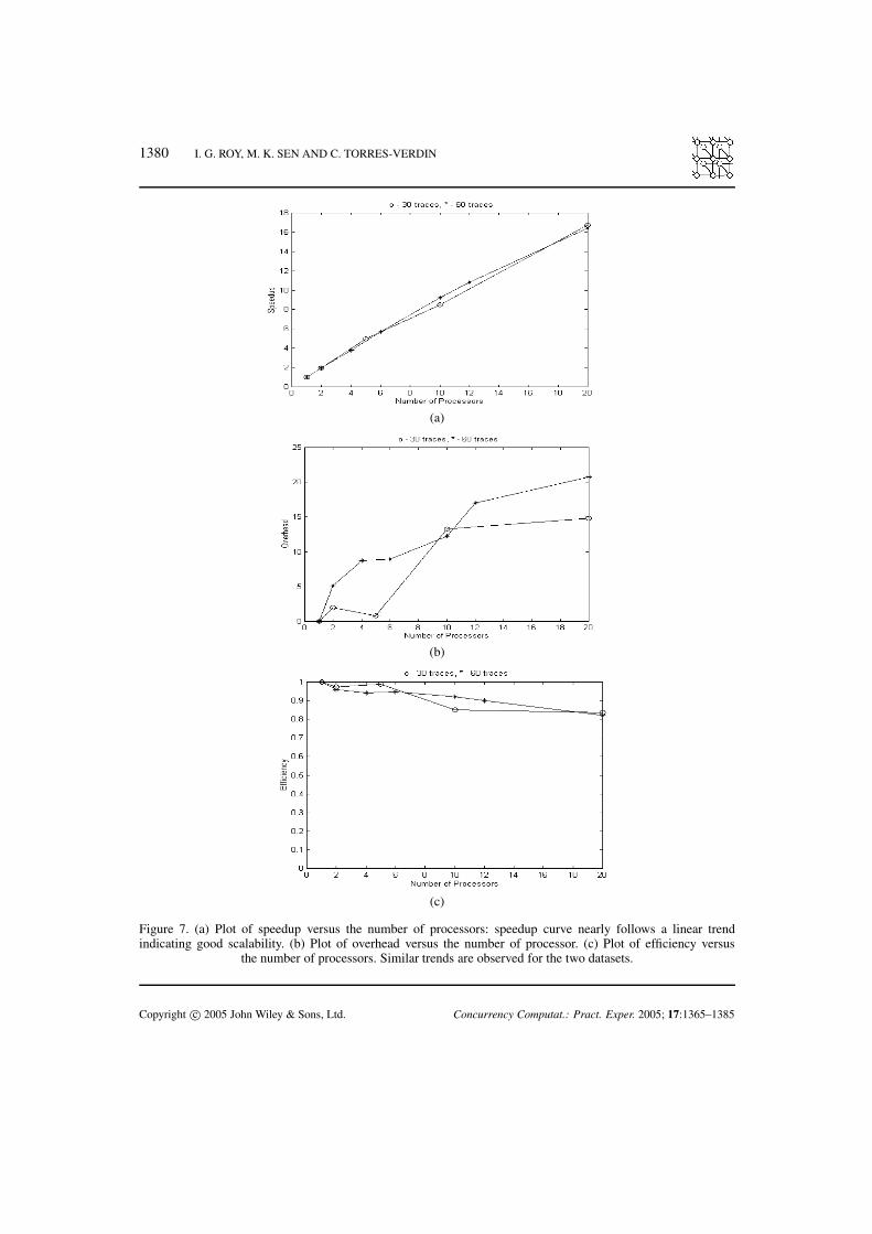
Figure 7. (a) Plot of speedup versus the number of processors: speedup curve nearly follows a linear trendindicating good scalability. (b) Plot of overhead versus the number of processor. (c) Plot of efficiency versus

the number of processors. Similar trends are observed for the two datasets.



0.00 0.00 0.00 0.00 0.00 0.00 0.00 0.00 0.00

0.000

0.500

1.000

1.500

2.000

seco

nds

km

Line 1 C:\MyData\seismic\prestack\GasModel\2000_noise\data_all.dir

0.0

0.5

1.0

1.5

2.0

Tim

e (

s)I II III

0.0 0.1 0.2 0.3 0.0 0.1 0.2 0.3 0.0 0.1 0.2 0.3

p (s/Km) p (s/Km) p (s/Km)

(a)

2 2.4 2.8 3.2

2

1.8

1.6

1.4

1.2

1

1 3 5 0 0.2 0.4

Tim

e (s

)

Vp Zp

Km/s (Kg/sm2)X106

(b)

Figure 8. Plot of data-fit presented in three panels: the left panel is observed data, the middle panelis the best fit data and the right panel is the data residual. (b) Plots of true (full curve), initial guess

(dashed curve), and the inverted model (dotted curve).

In an alternative definition due to Amdahl [34], if a parallel algorithm A is such that part of it, say α

fraction (known as the Amdahl fraction), is not parallelizable, then the speedup S(P ) is given by

S(P ) = P

1 + (P − 1)α(20)



Figure 9. Inversion results on field data. Data presented in the figure are described in the plane-wavedomain. The left panel is the observed seismic gather, the middle panel is the computed seismicgather for the inverted model and the right-most panel shows the inverted acoustic impedance and

Poisson’s ratio profiles. The interpreted gas zone is marked with arrows.

The above equation suggests that the speedup can attain the maximum value 1/α no matter how manyprocessors are used for parallel computation. Hence, if 5% of the algorithm is not parallelizable, thenthe maximum possible speedup is 20. In a most ideal situation, when α ≈ 0, the curve of speedupversus number of processors follows a linear trend else it deviates to a sublinear trend and maysaturate normally. The above definition of speedup thus provides the basis for selecting an optimalnumber of processors for parallel algorithm. Interestingly, with a given problem size, the efficiency(which is a measure of average fraction of time that each processor effectively uses while running aparallel algorithm) decreases with an increase in the number of processors. Note that as the number ofprocessors increases, inter-processor communication cost, idle time due to synchronization, etc. [35],increase; this is expressed in terms of a metric called overhead, which is defined as

Overhead = PT(P ) − T (1) (21)



Therefore, there exists a functional relationship between efficiency and overhead and this is expressedas

E(P) = T (1)

PT (P )= 1

1 + Overhead/T (1)(22)

Thus, while the overhead increases, the efficiency of the parallel architecture decreases. However,substantial reduction of overhead can be achieved by increasing the granularity, which is ameasure of the amount of computational work done before the processors have to communicate.Figures 7(a)–(c) are the plots of speedup, overhead and efficiency versus number of processors for thetwo sets of synthetic data. The speedup curve demonstrates a near linear trend, which indicates a goodscalability of the algorithm and suggests that only a small fraction of the code used is not parallelizable.We have found that only about 2% of our code is not parallelizable. A full-scale parallelization ofan algorithm for a highly nonlinear inverse problem is difficult to achieve unless the algorithm isintrinsically decomposable. Nevertheless, in most practical situations, full-scale decomposition andparallelization of an algorithm is not advisable as overhead grows considerably with the addition ofprocessors. We observe (Figure 7(b)) that the overhead is minimal using five processors and it increaseswith increasing numbers of processors. However, if the problem size increases on a fixed number ofprocessors, efficiency increases. We may keep the efficiency fixed and increase the problem size andthe number of processors, as overhead increases less quickly than problem size. This indicates goodscalability of our algorithm [36,37].

5. RESULTS

We have applied the inversion algorithm to both synthetic and field seismic data. Inversion resultsfor the synthetic example shown in Figure 5 are presented in Figures 8(a) and (b). Note that data-fit is excellent, and so is the model recovery. Convergence was reached in 50 iterations. The resultsobtained are in good agreement with the true model. In Figure 9, we present the inversion results forone CMP gather taken from a seismic survey line from the Gulf of Thailand. The normal move out(NMO) corrected observed and computed seismic gathers obtained after inversion and the invertedmodel with acoustic impedance (the product of the compressional wave velocity and density) andPoisson’s ratio are plotted in the same panel for the sake of comparison and interpretation. The zoneof low acoustic impedance and low Poisson’s ratio (marked by arrows in the figure) possibly containsfree gas in the formation. Detailed inversion results of the entire two-dimensional line from Gulf ofThailand including a correlation with well-log, are reported in [38].

6. CONCLUSIONS

We have designed an efficient gradient-based algorithm to invert large-scale pre-stack seismic datawithin an affordable time limit. Since the seismic inverse problem is extremely nonlinear and highlyill-posed, we adopt an adaptively RGN method that introduces stability and robustness of the gradient-based optimization technique. We have discussed various issues of parallel programming and thenmodified a sequential inversion algorithm to run on a parallel platform. Our parallel algorithm usesDMPC architecture connected with a high-speed network. The tests on parallelism indicate that ourparallel algorithm shows a sufficient speedup, allowing us to invert a large volume of seismic data(see [38]).



ACKNOWLEDGEMENTS

This work was supported by U.S. Department of Energy contract number #DE-FC26-00BC15305. We thankUnocal Corporation for providing us with the field dataset. We thank three anonymous reviewers and the editorsMalgo Peszynska and Mary Wheeler for their constructive criticisms of our paper.

REFERENCES

1. Highnam PT, Pieprzak A. Implementation of fast 3-D migration on a massively parallel computer. Proceedings of 61stAnnual International Meeting of Society of Exploration Geophysicists, 1991; 338–340.

2. Chang H, VanDyke JP, Solano M, McMechan GA, Epili D. 3-D prestack Kirchhoff depth migration: From prototype toproduction in a massively parallel processor environment. Geophysics 1998; 63:546–556.

3. Sen V, Sen MK, Stoffa PL. PVM based 3-D Kirchhoff depth migration using dynamically computed travel times:An application in seismic data processing. Parallel Computing 1999; 25:231–248.

4. Furumara T, Kennet BLN, Takenaka H. Parallel 3-D pseudospectral simulation of seismic wave propagation. Geophysics1998; 63:279–288.

5. Minkoff SE. Spatial parallelism of a 3D finite difference velocity–stress elastic wave propagation code. SIAM Journal onScientific Computing 2002; 24:1–19.

6. Kern M, Symes WW. Loop level parallelization of a seismic inversion codes. Proceedings of 63rd Annual InternationalMeeting of Society of Exploration Geophysicists, Tulsa, OK, 1993; 189–192.

7. Minkoff SE, Symes WW. Full waveform inversion of marine reflection data in plane-wave domain. Geophysics 1997;62(2):540–553.

8. Sen MK, Stoffa PL. Nonlinear one-dimensional seismic waveform inversion using simulated annealing. Geophysics 1991;56:1624–1638.

9. Aki K, Richards PG. Quantitative Seismology. W. H. Freeman: San Francisco, CA, 1980.10. Kennett BLN. Seismic Wave Propagation in Stratified Media. Cambridge University Press: Cambridge, 1984.11. Randall GE. Efficient calculation of differential seismograms for lithospheric receiver functions. Geophysical Journal

International 1989; 99:469–481.12. Sen MK, Roy IG. Computation of differential seismograms and iteration adaptive regularization in pre-stack waveform

inversion. Geophysics 2003; 6:2026–2039.13. Tarantola A. Inverse Problem Theory: Methods of Data Fitting and Model Parameter Estimation. Elsevier: Amsterdam,

1987.14. Engl HW, Hanke M, Neubauer A. Regularization of Inverse Problems. Kluwer: Dordrecht, 1996.15. Engl HW, Kunisch K, Neubauer A. Optimal a posteriori parameter choice for Tikhonov regularization for solving nonlinear

ill-posed problems. SIAM Journal of Numerical Analysis 1993; 30:1796–1838.16. Ramlau R. A steepest descent algorithm for the global minimization of the Tikhonov functional. Inverse Problems 2002;

18:381–403.17. Roy IG. A robust descent type algorithm for geophysical inversion through adaptive regularization. Applied Mathematical

Modelling 2002; 26:610–634.18. Morozov VA. Methods for Solving Incorrectly Posed Problems. Springer: New York, 1986.19. Ramlau R. Morozov’s discrepancy principle for Tikhonov regularization of nonlinear operators. Numerical Functional

Analysis and Optimization 2002; 23(1–2):147–172.20. Engl HW. Discrepancy principles of Tikhonov regularization of ill-posed problems leading to optimal convergence rates.

Journal of Optimization Theory and Applications 1987; 52:209–215.21. Coppersmith D, Winograd S. Matrix multiplication via arithmetic progressions. Journal of Symbolic Computing 1990;

9:251–280.22. Li K. Scalable parallel matrix multiplication on distributed memory parallel computers. Journal of Parallel and Distributed

Computing 2001; 61:1709–1731.23. Nash SG. A survey of truncated Newton methods. Journal of Computational and Applied Mathematics 2000; 124:45–59.24. Dembo RS, Steihaug T. Truncated-Newton algorithms for large scale unconstrained optimization. Mathematical

Programming 1983; 26:190–212.25. Nash SG. Preconditioning of truncated-Newton methods. SIAM Journal of Scientific and Statistical Computing 1985;

6:599–616.26. Nash SG, Nocedal J. A numerical study of the limited memory BFGS method and the truncated-Newton method for large-

scale optimization. SIAM Journal of Optimization 1991; 1:358–372.



27. Zou X, Navon IM, Berger M, Phua PKH, Schlick T, Le Dimet FX. Numerical experience with limited-memory andtruncated Newton methods. SIAM Journal of Optimization 1993; 3:582–608.

28. Hanke M. Regularizing properties of a truncated Newton-CG algorithm for nonlinear inverse problems. NumericalFunctional Analysis and Optimization 1997; 18:971–993.

29. Schnabel RB. A view of the limitation and opportunities and challenges in parallel nonlinear optimization. ParallelComputing 1995; 21(6):875–905.

30. Dubey PK, Adams GB, Flynn JM. Evaluating performance tradeoff between fine-grained and coarse-grained alternatives.IEEE Transactions on Parallel and Distributed Systems 1995; 6(1):17–27.

31. Eldred MS, Hart WE. Design and implementation of multilevel parallel optimization on the Intel teraflops. Paper AIAA-98-4707 in Proceedings of the 7th AIAA/USFA/NASA/ISSMO Symposium on Multidisciplinary Analysis and Optimization,1998; 44–54.

32. Snir M, Otto S, Huss-Lederman S, Walker D, Dongarra J. MPI: The Complete Reference. MIT Press: Cambridge, MA,1996.

33. Rauber T, Runger G, Wilhelm R. Deriving optimal data distributions for group parallel numerical algorithms. Proceedingson Programming Models for Massively Parallel Computers, Berlin, 9–12 October 1995, Giloi WK, Jahnichen S, Shriver BD(eds.).

34. Amdahl G. Keynote address. Proceedings of the 2nd International Supercomputer Conference, Santa Clara, CA, May 1987.35. Kumar V, Grama A, Gupta A, Karypis G. Introduction to Parallel Computing. Benjamin Cummings: New York, 1994.36. Gustafson JL, Montry GR, Benner RE. Development of parallel methods for a 1024 processor hypercube. SIAM Journal

on Scientific and Statistical Computing 1988; 9(4):609–638.37. Kumar V, Gupta A. Analyzing scalability of parallel algorithms and architectures. Journal of Parallel and Distributed

Computing 1994; 22:379–391.38. Roy IG, Sen MK, Torres-Verdin C, Varela OJ. Pre-stack inversion of Gulf of Thailand data. Geophysics 2004; 69(6):1470–

1477.


Full waveform seismic inversion using a distributed system ... · seismic inversion of a large...

Documents

Transcript of Full waveform seismic inversion using a distributed system ... · seismic inversion of a large...