Full-wave seismic illumination and resolution analyses:A Poynting-vector-based method

Zhe Yan1 and Xiao-Bi Xie2

ABSTRACT

Illumination and resolution analysis provides vital informationregarding the response of an imaging system to subsurface struc-tures. However, generating the resolution function is often com-putationally intensive, which prevents it from being widely used inpractice. This problem is particularly severe for the time-domainmigrationmethod, such as reverse time migration (RTM). To solvethis problem, we have developed a fast full-wave-based illumina-tion and resolution analysis method. The source- and receiver-sidewaves are extrapolated to the subsurface for simulating the imag-ing process. To create the relations linking the incident and scat-tering directions to the target wavenumber components, we haveadopted an efficient Poynting-vector-based method for wavefield

angle decomposition. By taking the approximation that the time-domain wavefield preserves the source spectrum during propaga-tion, massive input/output and trace-by-trace Fourier transformcan be avoided and the finite-frequency calculated broadband sig-nal can be directly converted to the wavenumber domain for cal-culating the point spreading functions (PSFs). Combining theseapproaches, the resulting method avoids intensive calculations,massive input/output, and huge storage requirements commonlyinvolved in generating the illumination and resolution functions.The method is highly efficient and particularly suitable to teamwith RTM for resolution analysis. Numerical examples are usedto validate this method. We have determined how to calculate theacquisition dip response and PSFs, based on which, the quality ofthe depth image can be significantly improved.

INTRODUCTION

Illumination analysis has been widely used in optimizing theacquisition system design, evaluating the image quality, and cor-recting for the distorted depth image caused by uneven illumination.To calculate the illumination measurement, the source and receiverwaves should be extrapolated to the subsurface target area. Theillumination and resolution calculations are closely related to thepropagation angles of incidence and scattering waves and the targetstructural dip angle. Therefore, the earlier illumination and resolu-tion analyses were built on ray-based methods because theynaturally provided directional information (Hubral et al., 1999;Schneider and Winbow, 1999; Bear et al., 2000; Muerdter andRatcliff, 2001; Gelius et al., 2002). However, the ray-based methodsare limited by the high-frequency asymptotic approximation (Hoff-mann, 2001); thus, the wave-equation-based methods were adoptedfor the illumination calculation.

Because the wave-equation-based methods do not explicitlyprovide the propagation direction, several methods were developedto extract angle information from the wavefield. These methods canbe separated under two categories. The first group uses the integralmethod, e.g., the local-plane wave decomposition and wavelettransform-based methods (Xie and Lay, 1994; Wu and Chen,2002, 2006; Xie and Wu, 2002; Mao et al., 2010), local Fouriertransform-based methods (Xu et al., 2010, 2011; Zhang et al.,2010), and methods that convert the local offset-domain image intolocal angle-domain image (de Bruin et al., 1990; Prucha et al., 1999;Sava and Fomel, 2003). The second group uses the differentialmethod, e.g., the Poynting-vector- or gradient-vector-based method(Yoon and Marfurt, 2006; Yoon et al., 2011; Zhang and McMechen,2011). The differential type methods require only the calculation ofspatial or temporal derivatives at given locations. Instead, the inte-gral type methods analyze the wavefield within a neighboringregion with the dimension of a wavelength. Therefore, the latter

Manuscript received by the Editor 2 January 2016; revised manuscript received 9 July 2016; published online 07 September 2016.1China University of Geosciences, Institute of Geophysics and Geomatics, Wuhan, China and University of California, IGPP, Santa Cruz, California, USA.

E-mail: yanzhe@cug.edu.cn.2University of California, IGPP, Santa Cruz, California, USA. E-mail: xxie@ucsc.edu.© 2016 Society of Exploration Geophysicists. All rights reserved.

S447

GEOPHYSICS, VOL. 81, NO. 6 (NOVEMBER-DECEMBER 2016); P. S447–S458, 11 FIGS.10.1190/GEO2016-0003.1

Dow

nloa

ded

09/1

3/16

to 1

28.1

14.6

9.14

2. R

edis

trib

utio

n su

bjec

t to

SEG

lice

nse

or c

opyr

ight

; see

Ter

ms

of U

se a

t http

://lib

rary

.seg

.org

/

involves more calculations and is much more time consuming.However, compared with the differential method, the integral meth-od is physically sound, more reliable, and can handle cases suchas multiply simultaneously arriving waves. Depending on the pur-poses, trade-offs between the accuracy and efficiency are often re-quired. Yan and Xie (2012) and Jin et al. (2014) review variousangle decomposition methods. These methods have been combinedwith the one-way propagator and successfully used in illuminationand resolution analyses (Wu and Chen, 2002, 2006; Jin and Wal-raven, 2003; Xie et al., 2003, 2006; Jin et al., 2006; Mao et al.,2010; Mao and Wu, 2011). Recently, along with the increasing ap-plications of the reverse time migration (RTM), there have been de-mands for the full-wave-based illumination analysis technique. Xieand Yang (2008) propose the illumination and resolution analysismethod based on the time-domain local slowness analysis. Cao andWu (2009a), Yan and Xie (2012), and Yan et al. (2014) propose theillumination method based on the frequency-domain angle decom-position. An alternative method, which first calculates the pointspreading function (PSF) by directly imaging a point scatter, fol-lowed by converting the PSF into the wavenumber domain for il-lumination analysis, was also proposed (Fletcher et al., 2012; Cao,2013; Chen and Xie, 2015; Valenciano et al., 2015).Illumination and resolution analysis provides useful information

for image correction. Rickett (2003) applies wave-equation-basedillumination analysis to normalize the depth image. Based on theray-tracing method, Gelius et al. (2002), Sjoeberg et al. (2003),and Lecomte (2008) derive the resolution function and use it to cor-rect the image in the wavenumber domain. Based on the one-waypropagator, Xie et al. (2005) propose to correct the image using thePSF. Wu et al. (2004, 2006), Cao and Wu (2009b), and Mao and Wu(2010) use the wavelet transform for illumination and resolutionanalysis. Fletcher et al. (2012) use the resolution for post image in-version. Yang et al. (2013) use an illumination compensation strategyfor wavefield tomography in the image domain. Cao (2013) and Yanet al. (2014) test image correction for the full-wave RTM image.In this paper, we propose an efficient illumination and resolution

analysis method under the full-wave frame, in which the angle-domain information is extracted using the Poynting vector. We firstbriefly review the relationship between the seismic image and theillumination and resolution functions. Then, we present the methodto calculate the local illumination matrix (LIM) and convert it to thePSF and the acquisition dip response (ADR). Numerical examplesare used to demonstrate the proposed method in illumination andresolution analysis.

METHODOLOGY

Using a survey system composed of a source at xs and a receiverat xg to investigate a small target region VðxÞ in the vicinity oflocation x, the seismic data recorded at xg can be expressed as(e.g., Wu et al., 2007)

Dðx;xg;xs;ωÞ¼sðωÞZVðxÞ

k20Gðx0;xs;ωÞMðx0ÞGðx0;xg;ωÞdx0;

(1)

where ω is the frequency, x 0 is the local coordinate defined insidethe VðxÞ, k0 ¼ ω∕c0ðxÞ is the local wavenumber, c0ðxÞ is the back-ground velocity, Mðx 0Þ ¼ δcðx 0Þ∕cðxÞ is the relative velocity per-

turbation, δcðx 0Þ is the velocity perturbation, sðωÞ is the sourcespectrum,Gðx 0; xs;ωÞ is the Green’s function propagating the wavefrom xs to the target at x 0, and Gðx 0; xg;ωÞ is the Green’s functionpropagating the wave from the target to the receiver at xg. Boththese Green’s functions are calculated in the background model,and the reciprocity Gðx 0; xg;ωÞ ¼ Gðxg; x 0;ωÞ is used. For an ac-quisition system composed of multiple sources and receivers, thedepth image at x 0 0 can be expressed as

Iðx; x 0 0;ωÞ ¼ sðωÞXxs

Xxg

Gðx 0 0; xs;ωÞ

×D�ðx; xg; xs;ωÞGðx 0 0; xg;ωÞ: (2)

Substituting equation 1 into equation 2, the depth image can beexpressed as (e.g., Xie et al., 2005; Yan et al., 2014)

Iðx; x 0 0;ωÞ ¼ZVðxÞ

Mðx 0ÞRðx; x 0; x 0 0;ωÞdx 0; (3)

where

Rðx;x0;x00;ωÞ¼2k20sðωÞs�ðωÞ×Xxs

Xxg

Gðx00;xs;ωÞG�ðx0;xs;ωÞG�ðx0;xg;ωÞGðx00;xg;ωÞ:

(4)

The resolution function Rðx; x 0; x 0 0Þ, through forward and back-ward propagations, maps the velocity perturbation at x 0 to the imageat x 0 0. Because of the limitations of the system, e.g., the incompleteacquisition aperture or the error in migration velocity model, it maynot exactly map the perturbation to its original location, causing theimage smearing. Thus, Rðx; x 0; x 0 0Þ is also known as the PSF that isthe response of the imaging system to a point scatter (Chen andSchuster, 1999; Gelius et al., 2002; Gibson and Tzimeas, 2002; Xieet al., 2005). Equation 3 is similar to a convolution, i.e., the PSFconvolving with the velocity perturbation to give the image. How-ever, Rðx; x 0; x 0 0Þ is localized; i.e., it is defined near location x andvaries in the space due to the variable illumination. Introducing thelocal Fourier transform over VðxÞ, the space convolution in equa-tion 3 can be converted into the multiplication in the wavenumberdomain kd ¼ ks þ kg (Gelius et al., 2002; Xie et al., 2005)

Iðx; kd;ωÞ ¼ Rðx; kd;ωÞ · Mðx; kdÞ; (5)

where

Mðx; kdÞ ¼ZVðxÞ

Mðx 0Þeikd ·x 0dx 0; (6)

Rðx; kd;ωÞ ¼ 2k20sðωÞs�ðωÞXxs

Xxg

Aðx; kd; xs; xg;ωÞ;

(7)

and

S448 Yan and Xie

Dow

nloa

ded

09/1

3/16

to 1

28.1

14.6

9.14

2. R

edis

trib

utio

n su

bjec

t to

SEG

lice

nse

or c

opyr

ight

; see

Ter

ms

of U

se a

t http

://lib

rary

.seg

.org

/

Aðx;kd;xs;xg;ωÞ ←kd¼ksþkg

G�ðx;ks;xs;ωÞG�ðx;kg;xg;ωÞGðx;ks;xs;ωÞGðx;kg;xg;ωÞ;(8)

where kd ¼ ks þ kg is the wavenumber related to structural dip, ksand kg are the incident and scattered wavenumbers near the imagepoint, and Rðx; kd;ωÞ is the wavenumber-domain PSF. The map-ping in equation 8 converts the response from ðks; kgÞ, the wave-number domain in acquisition coordinate, to kd, the wavenumberdomain in target coordinate (refer to Figure 1).Given the acquisition system and the overburden structure, meth-

ods have been proposed to calculate Rðx; kdÞ or Rðx; x 0Þ, followedby using it in seismic illumination and resolution analyses (Xieet al., 2006; Lecomte, 2008). It is relatively straightforward to cal-culate the Rðx; kdÞ using the frequency-domain method. For a time-domain method such as the finite difference, theoretically, one canuse Fourier transform to convert the entire time-space wavefield intofrequency domain. Then, the wavefield can be decomposed into itswavenumber component by using the local slant stacking or localfast Fourier transform (FFT), followed by calculating the PSF usingequations 7 and 8 (Yan et al. 2014). However, such a procedureoften involves intensive calculations, huge input/output, and storageand is computationally inefficient. Instead, we propose using thePoynting vector to decompose the wavefield into its angle compo-nent directly in time domain. Then, by assuming the frequency con-tents are unchanged during the propagation, the broadband signalcan be directly converted into its frequency component. Finally, thisfrequency-angle-domain information is used in equations 7 and 8 tocreate the PSF. The resulted method is highly efficient.Given a broadband source time function, such as a Ricker wave-

let, the finite-difference calculated wavefield can be expressed as

uðx; xs; tÞ ¼Z

sðωÞGðx; xs;ωÞe−iωtdω: (9)

Using the Poynting vector method, the source wavefield canbe decomposed into a superposition of local beams uðx; xs; tÞ ¼P

θsuðx; θs; xs; tÞ, where θs is the local incident angle, and

uðx; θs; xs; tÞ ¼Z

sðωÞGðx; θs; xs;ωÞe−iωtdω: (10)

We calculate the average mean square amplitude of equation 10within a short time interval T

1

T

Zu2ðx;θs;xs;tÞdt

¼Z

sðωÞs�ðωÞGðx;θs;xs;ωÞG�ðx;θs;xs;ωÞdω: (11)

Assuming that, during the propagation, the wavefield keeps itsspectrum unchanged, we have

Gðx; θs; xs;ωÞG�ðx; θs; xs;ωÞ

¼ 1

TR ½sðωÞs�ðωÞ�dω

Zu2ðx; θs; xs; tÞdt: (12)

Similarly, for receiver-side wave, we have

Gðx; θg; xg;ωÞG�ðx; θg; xg;ωÞ

¼ 1

TR ½sðωÞs�ðωÞ�dω

Zu2ðx; θg; xg; tÞdt; (13)

where θg is the local scattered angle.From equations 12 and 13, we can create the LIM for the acquis-

ition system (Xie et al., 2006)

LIMðx;θs;θg;ωÞ¼2k20sðωÞs�ðωÞXxs

Xxg

Aðx;θs;θg;xs;xg;ωÞ;

(14)

where

Aðx;θs;θg;xs;xg;ωÞ¼G�ðx;θs;xs;ωÞG�ðx;θg;xg;ωÞGðx;θs;xs;ωÞGðx;θg;xg;ωÞ;

¼ 1

T2nR ½sðωÞs�ðωÞ�dωo2

Zu2ðx;θs;xs;tÞdt

×Z

u2ðx;θg;xg;tÞdt: (15)

The LIMðx; θs; θg;ωÞ can be directly calculated from the time-domain wavefield. We convert it to Rðx; kd;ωÞ for resolution analy-sis. The LIM (equations 14 and 15) is similar to the PSF in equa-tions 7 and 8, except that the former decomposes the illuminationinto the incidence/scattering angle domain θs and θg, and the latterdecomposes the illumination into dip wavenumber domain kd. In-tegrating their components sums up all angle-dependent illumina-tion together, and the two should be equivalent with each other.Therefore, we integrate equation 15 with respect to dθsdθg and thenconvert variables from ðθs; θgÞ to ðkd; θdÞZ

Aðx; θs; θg; xs; xg;ωÞdθsdθg

¼Z

Aðx; kd; θd; xs; xg;ωÞJ�∂ðθs; θgÞ∂ðkd; θdÞ

�dkddθd; (16)

Figure 1. Cartoon showing the coordinate system.

Illumination and resolution analysis S449

Dow

nloa

ded

09/1

3/16

to 1

28.1

14.6

9.14

2. R

edis

trib

utio

n su

bjec

t to

SEG

lice

nse

or c

opyr

ight

; see

Ter

ms

of U

se a

t http

://lib

rary

.seg

.org

/

where kd ¼ jkdj and θd is the dipping angle, J½∂ðθs; θgÞ∕∂ðkd; θdÞ�is the Jacobian. The coordinate transforms involve first rotatingthe incident/scattering angles ðθs; θgÞ to dipping/reflection anglesðθd; θrÞ with θd ¼ ðθs þ θgÞ∕2 and θr ¼ ðθs − θgÞ∕2 (refer toFigure 1), followed by converting them to the dipping wavenumberdomain ðkd; θdÞ with kd ¼ 2k0 cos θr and θd ¼ θd (refer to Alkha-lifah, 2015; Xie, 2015). The two transforms can be combined into(

θs ¼ θd þ cos−1ð kd2k0

Þ;θg ¼ θd − cos−1ð kd

2k0Þ: (17)

The Jacobian is

J

�∂ðθs; θgÞ∂ðkd; θdÞ

�¼ 1

k0

ffiffiffiffiffiffiffiffiffiffiffiffiffiffiffiffiffiffiffiffiffi1 −

�kd2k0

�2

r : (18)

Thus, we have

Aðx;kd;xs;xg;ωÞ

¼A

�x;�θdþcos−1

�kd2k0

�;

�θd−cos−1

�kd2k0

�;xs;xg;ω

×1

k0

ffiffiffiffiffiffiffiffiffiffiffiffiffiffiffiffiffiffiffi1−

�kd2k0

�2

r : (19)

Substituting equation 15 into equation 19, and then into equa-tion 7, the PSF can be calculated from the LIM

Rðx; kd;ωÞ ¼2sðωÞs�ðωÞk20

T2

�R ½sðωÞs�ðωÞ�dω2

×Xxs

Xxg

�Zu2�x;�θd þ cos−1

�kd2k0

�; xs; t

dt

×Z

u2�x;�θd − cos−1

�kd2k0

�; xg; t

dt

×1

k0

ffiffiffiffiffiffiffiffiffiffiffiffiffiffiffiffiffiffiffiffiffi1 −

�kd2k0

�2

r : (20)

Illumination response for a locally planar reflector at target loca-tion x with a dipping angle θd is defined as the ADR (Wu et al.,2003; Xie et al., 2006), which can be calculated from the LIM

ADRðx;θdÞ¼Z

LIM

�x;θdþθr

2;θd−θr

2;ω

dθrdω: (21)

THE POYNTING VECTOR METHOD

Poynting vector gives the wave energy flux direction. Therefore,by calculating the Poynting vector, we can obtain the wave propa-

gation direction at a given time and space location. For scalar waveequation, the Poynting vector can be calculated as (Yoon et al.,2004, 2011; Yoon and Marfurt, 2006)

p ¼ −∂u∂t

· ∇u; (22)

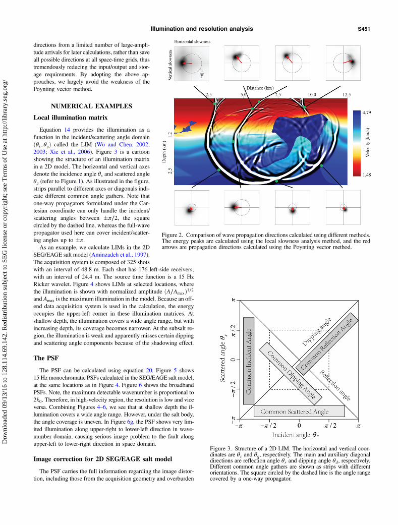
where u is the finite-difference calculated wavefield and∇u is its spatialgradient. In a staggered-grid finite-difference scheme, the time deriva-tive and spatial gradient are intermediate variables that can be obtainedwithout extra effort. Thus, the resulted method is highly efficient andwidely used for several purposes. Yoon et al. (2004) and Pestana et al.(2014) use the Poynting vector method to eliminate the low-wavenum-ber artifacts in the RTM image. Dickens and Winbow (2011) use thismethod to generate common angle image gathers in RTM. Wang et al.(2013) test the Poynting vector method in illumination analysis, andXie (2015) uses this method in the full-waveform inversion.To compare different angle measurement methods, we calculate

the wave propagation directions in the BP salt model (Billette andBrandsberg-Dahl, 2005) using the local slowness analysis method(Xie and Lay, 1994; Yan and Xie, 2012; Yan et al., 2014) and thePoynting vector method, and the result is shown in Figure 2. Thelocations of energy peaks from slowness analysis give the slownessvectors, which provide the wave propagation directions. The redarrows give propagation directions calculated using the Poyntingvector method. At space-time locations where only one wavefrontis encountered, the estimated directions by both methods are consis-tent. However, if more than one wavefront coexist, slowness analysismethod can give propagation directions of individual waves, whereasthe Poynting vector method can only provide one single propagationdirection, which may be incorrect. Jin et al. (2014) indicate that thewave propagation direction estimated using the Poynting vectormethod may be unreliable under low amplitudes. To improve its reli-ability, certain methods were proposed, e.g., averaging the resultsover multiple time steps (Yoon et al., 2011), smoothing the Poyntingvectors in the space domain (Dickens and Winbow, 2011), using aleast-squares solution over the time or space (Yan and Ross, 2013), orusing the optical flow method to stabilize Poynting vector directions(Vyas et al., 2011; Zhang, 2014). All these methods can improve theaccuracy but often with large computation and/or storage cost.Although the Poynting vector method can encounter certain dif-

ficulties in a complicated wavefield, these situations usually onlyaccount for a very small portion in the entire space-time domainduring the wave propagation process. Unlike in the migration, theillumination calculation does not involve the “data.” To simulate thepropagation effect from the receiver side, we use the simple impulseas the “fictitious” data, which is injected from individual receiverlocations one after another. Thus, the receiver-side extrapolation issimply calculating a Green’s function from the receiver location,exactly the same as dealing with a source. This largely relaxes therequirement of dealing with complex situations. To further improvethe stability, we limit our measurement to within several time win-dows with most energetic arrivals. This can be easily accomplishedby scanning the wavefield twice, locating the time windows in thefirst scan, and measuring the wave propagation directions and meansquare amplitudes in located time windows in the second scan. InRTM imaging, to correlate with the time-reversed receiver wave-field, the source wavefield needs to be stored or regenerated. There-fore, the scanning procedure does not require additional calculation.In addition, this method only saves mean square amplitudes and

S450 Yan and Xie

Dow

nloa

ded

09/1

3/16

to 1

28.1

14.6

9.14

2. R

edis

trib

utio

n su

bjec

t to

SEG

lice

nse

or c

opyr

ight

; see

Ter

ms

of U

se a

t http

://lib

rary

.seg

.org

/

directions from a limited number of large-ampli-tude arrivals for later calculations, rather than saveall possible directions at all space-time grids, thustremendously reducing the input/output and stor-age requirements. By adopting the above ap-proaches, we largely avoid the weakness of thePoynting vector method.

NUMERICAL EXAMPLES

Local illumination matrix

Equation 14 provides the illumination as afunction in the incident/scattering angle domainðθs; θgÞ called the LIM (Wu and Chen, 2002,2003; Xie et al., 2006). Figure 3 is a cartoonshowing the structure of an illumination matrixin a 2D model. The horizontal and vertical axesdenote the incidence angle θs and scattered angleθg (refer to Figure 1). As illustrated in the figure,strips parallel to different axes or diagonals indi-cate different common angle gathers. Note thatone-way propagators formulated under the Car-tesian coordinate can only handle the incident/scattering angles between �π∕2, the squarecircled by the dashed line, whereas the full-wavepropagator used here can cover incident/scatter-ing angles up to �π.As an example, we calculate LIMs in the 2D

SEG/EAGE salt model (Aminzadeh et al., 1997).The acquisition system is composed of 325 shotswith an interval of 48.8 m. Each shot has 176 left-side receivers,with an interval of 24.4 m. The source time function is a 15 HzRicker wavelet. Figure 4 shows LIMs at selected locations, wherethe illumination is shown with normalized amplitude ðA∕AmaxÞ1∕2and Amax is the maximum illumination in the model. Because an off-end data acquisition system is used in the calculation, the energyoccupies the upper-left corner in these illumination matrices. Atshallow depth, the illumination covers a wide angle range, but withincreasing depth, its coverage becomes narrower. At the subsalt re-gion, the illumination is weak and apparently misses certain dippingand scattering angle components because of the shadowing effect.

The PSF

The PSF can be calculated using equation 20. Figure 5 shows15 Hz monochromatic PSFs calculated in the SEG/EAGE salt model,at the same locations as in Figure 4. Figure 6 shows the broadbandPSFs. Note, the maximum detectable wavenumber is proportional to2k0. Therefore, in high-velocity region, the resolution is low and viceversa. Combining Figures 4–6, we see that at shallow depth the il-lumination covers a wide angle range. However, under the salt body,the angle coverage is uneven. In Figure 6g, the PSF shows very lim-ited illumination along upper-right to lower-left direction in wave-number domain, causing serious image problem to the fault alongupper-left to lower-right direction in space domain.

Image correction for 2D SEG/EAGE salt model

The PSF carries the full information regarding the image distor-tion, including those from the acquisition geometry and overburden

Figure 2. Comparison of wave propagation directions calculated using different methods.The energy peaks are calculated using the local slowness analysis method, and the redarrows are propagation directions calculated using the Poynting vector method.

Figure 3. Structure of a 2D LIM. The horizontal and vertical coor-dinates are θs and θg, respectively. The main and auxiliary diagonaldirections are reflection angle θr and dipping angle θd, respectively.Different common angle gathers are shown as strips with differentorientations. The square circled by the dashed line is the angle rangecovered by a one-way propagator.

Illumination and resolution analysis S451

Dow

nloa

ded

09/1

3/16

to 1

28.1

14.6

9.14

2. R

edis

trib

utio

n su

bjec

t to

SEG

lice

nse

or c

opyr

ight

; see

Ter

ms

of U

se a

t http

://lib

rary

.seg

.org

/

structures. According to equation 5, the imagecan be seen as a convolution between the PSFand the velocity perturbation. Ideally, by decon-volving the PSF from the image in space domainor by dividing PSF from the image in wavenum-ber domain, the uneven illumination can be com-pensated, and the overall quality of the image canbe improved.As the first example, we apply the illumination

and resolution analysis to the 2D SEG/EAGE saltmodel. To conduct the image correction, we firstdecompose the source and receiver waves intolocal beams using equations 12 and 13. Then, useequations 14 and 15 to create LIMs as shown inFigure 3. Using equations 19 and 20, the LIMsare converted to PSFs, which are shown in Fig-ure 6. Finally, by using a 2D sampling functionwith cosine tapers and the windowed FFT, thedepth image is transformed to the local wave-number domain and corrected by the PSF. Theabove-mentioned process is demonstrated in Fig-ure 7. Figure 7a shows the conventional RTMimage. The acquisition system is the same as thatused in generating Figure 4. The area markedby the white square is chosen to demonstratethe procedure of image correction. In the middle,from left to right are the conventional imagesampled by the white square (Figure 7b), thewavenumber spectrum of the conventional image(Figure 7c), the wavenumber-domain PSF (Fig-ure 7d), the corrected spectrum computed by di-viding panel (c) by panel (d) (Figure 7e), andcorrected space-domain image (Figure 7f). In Fig-ure 7b, from upper left to lower right is the imageof the fault. Along the upper-right to lower-leftdirection are several artifacts caused by internalmultiples. In Figure 7d, we see strong illuminationalong the upper-left to the lower-right direction inthewavenumber domain. The uneven illuminationweakens the image of the fault and enhancesartifacts. In Figure 7e, after correction, the wave-number spectrum for the fault is enhanced,whereas the spectrum for the artifacts is effec-tively suppressed. After converting back to thespace domain, the image for the fault is largelyimproved. Using the sampling window to scanthe entire image and repeatedly using the correc-tion process mentioned above, we obtain thecorrected image shown in Figure 7g. ComparingFigure 7a and 7g, subsalt structures in the cor-rected image are more balanced, and severalsteep-dip structures are more emphasized. As acomparison, we apply automatic gain control(AGC) to the conventional RTM, and the resultis shown in Figure 7h. By comparing with Fig-ure 7a, the AGC can raise the image amplitudeat a deeper depth. However, comparing with Fig-ure 7g, the AGC result cannot match the quality ofthe illumination corrected image. The image in the

Figure 4. Local illumination matrices at selected locations in the 2D SEG/EAGE saltmodel. At the shallow part, the target is illuminated by wide aperture, but the aperturebecomes narrower with the increase of the depth. At the subsalt region, the energy isgenerally weak and apparently misses certain angle components due to the shadowingeffect.

Figure 5. Wavenumber-domain PSF at selected locations in the 2D SEG/EAGE saltmodel, calculated using the single (dominant) frequency signal.

S452 Yan and Xie

Dow

nloa

ded

09/1

3/16

to 1

28.1

14.6

9.14

2. R

edis

trib

utio

n su

bjec

t to

SEG

lice

nse

or c

opyr

ight

; see

Ter

ms

of U

se a

t http

://lib

rary

.seg

.org

/

Figure 7. (a) The conventional RTM image forthe 2D SEG/EAGE salt model, in which the areamarked by a white square is chosen to demonstratethe correction procedure. (b) The original image,(c) its wavenumber spectrum, (d) wavenumber-do-main PSF, (e) corrected spectrum, and (f) correctedimage. The entire corrected image is shown in (g).(h) The conventional RTM image with the AGC.

Figure 6. Wavenumber-domain PSF at selectedlocations in the 2D SEG/EAGE salt model, calcu-lated using the broadband signal.

Illumination and resolution analysis S453

Dow

nloa

ded

09/1

3/16

to 1

28.1

14.6

9.14

2. R

edis

trib

utio

n su

bjec

t to

SEG

lice

nse

or c

opyr

ight

; see

Ter

ms

of U

se a

t http

://lib

rary

.seg

.org

/

subsalt area is still weak, and some steeply dipping structures aremissing.The image can also be corrected using the ADR maps in the dip

angle domain (Wu et al., 2004; Mao and Wu, 2011; Yan et al.,2014). First, we apply the FFT to transform the conventionalRTM image shown in Figure 7a to wavenumber domain, in whichthe image is divided into 24 equal-sized fan-shaped areas, each oc-cupying a 15° interval and using its center angle as the nominal dipangle. Using inverse FFT, the images in individual wedges are trans-formed back to space domain to form 24 common dip angle images.Figure 8c and 8d shows two examples at θd ¼ 45° and 45°. Second,we calculate ADR maps using equation 21, and two correspondingexamples are shown in Figure 8a and 8b. The common dip imagesare corrected by dividing the correspondent ADRs, and the resultsare shown in Figure 8e and 8f. Finally, sum up all 24 ADR correctedcommon dip images to obtain the corrected image, which is shownin Figure 8g. Comparing Figures 7g and 8g, image corrected usingthe ADR is usually less accurate as that using the PSF because theformer uses only the information in dip angle θd, but the latter fur-ther uses the scale information in kd.

Image correction for the Sigsbee 2A velocity model

In this example, we investigate the Sigsbee 2A salt model(Paffenholz et al., 2002). The acquisition system is composed of

500 shots with a source interval of 45.7 m. Minimum and maximumoffsets are 0 and 7932 m, respectively, and the receiver interval is22.9 m. The source is a 20 Hz Ricker wavelet. The conventionalRTM image is shown in Figure 9a. Because subsalt structuresare nearly horizontal, shown in Figure 9b is the 0° ADR map, whichis generated by half of the sources and receivers used for the RTM.From the ADR map, we see that near-horizontal structures belowthe overhang part of the salt body are poorly illuminated. Theseareas are responsible for the missing image in the RTM result(circled by ellipses). Similar to the previous example, we use thePSF to correct the RTM image, and the result is shown in Figure 10a.Compared with the conventional RTM image in Figure 9a, the im-age quality is significantly improved. In general, the amplitudes aremore balanced, particularly in the subsalt region. By magnificationin the areas labeled by white squares, Figure 10b and 10d shows theenlarged details in the corrected image. Compared with the conven-tional images shown in Figure 10c and 10e, the corrected imageshave consistent layered structures that can be traced to closer to thesalt flank, improved focusing to point like scatters, and generallysharper images. Comparing Figure 10a with Figure 9a, the correc-tion also removes long-wavelength artifacts in the image (can alsobe shown in Figure 7). At shallow depth, the PSFs have very strongnear-zero-wavenumber components generated by diving waves, thesame source causing the low-wavenumber artifacts. After dividing

Figure 8. (a and b) The −45° and 45° ADR maps, (c and d) correspondent common-dip images, (e and f) common-dip images after ADRcorrection, and (g) the final image after summing up partial images for all dipping angles.

S454 Yan and Xie

Dow

nloa

ded

09/1

3/16

to 1

28.1

14.6

9.14

2. R

edis

trib

utio

n su

bjec

t to

SEG

lice

nse

or c

opyr

ight

; see

Ter

ms

of U

se a

t http

://lib

rary

.seg

.org

/

the PSF in wavenumber domain, low-wavenumber artifacts are ef-fectively eliminated from the image.

COMPUTATIONAL ISSUES AND THE EFFICIENCYOF THE METHOD

From the formulations of the illumination and resolution analy-sis, we see that intensive computations are required to calculateGreen’s functions and decompose the wavefield into angle compo-nents. In RTM imaging, the wavefield needs to be extrapolated fromsources to the subsurface. If the illumination and resolution analysisis accompanying the imaging (e.g., for related quality control or im-age correction purpose), we actually use the existing source wave-fields as the Green’s functions without having to recalculate them.In the resolution calculation, one of the important steps is convertingthe measurement from the incident/scattering angle domain to dip-ping wavenumber domain (equation 20). Because ðθs; θgÞ andðkd; θdÞ are defined in discretized grids, proper interpolations shouldbe adopted.The illumination and resolution related functions, the LIM, PSF,

and ADR, are all slowly varying functions. We can use a coarser gridto calculate these functions and use interpolation to extend them tothe entire model. In addition because the illumination calculationis intrinsically a modeling, there is no noise being involved. Their

calculations usually do not need as much of sources and receiversused in a RTM. Taking the 2D SEG/EAGE salt model as an example,we calculate the 45° ADRmap using different grid sizes and numbersof sources and receivers. The results are shown in Figure 11, in whichFigure 11a shows the ADR calculated for all grid points using allsources and receivers as used in the RTM. Figure 11b shows theADR calculated for a 2 × 2 interval, and interpolated to every point.Figure 11c shows the ADR calculated for a 3 × 3 interval, and inter-polated to every point. We see even using the 3 × 3 interval, the resultis still acceptable. Note that in a 3D case, using the 2 × 2 × 2 intervalcan cut the calculation and storage to one-eighth, and using the 3 ×3 × 3 interval can cut the cost to 1/27. Figure 11d and 11e showsADRs calculated using one-half and one-quarter of the sources

Figure 9. (a) The conventional RTM image of the Sigsbee 2Amodel and (b) the ADR map for horizontal (zero dipping angle)reflector.

Figure 10. (a) Corrected RTM image by deconvolving with thePSF. To illustrate the details, (b and d) are enlarged corrected im-ages indicated by white squares in (a), and (c and e) are originalimages at the same area.

Illumination and resolution analysis S455

Dow

nloa

ded

09/1

3/16

to 1

28.1

14.6

9.14

2. R

edis

trib

utio

n su

bjec

t to

SEG

lice

nse

or c

opyr

ight

; see

Ter

ms

of U

se a

t http

://lib

rary

.seg

.org

/

and receivers. The results show that, even with one quarter of thesources and receivers, the generated ADR maps are still reasonablyaccurate, except at very shallow depth. In correcting the RTM imageusing the PSF, we actually sample the image using a 21 × 21 spacewindow. After correction, we use 5 × 5 corrected pixels at the centerof the sampling window to reconstruct the corrected image. Then,move the sampling window according to a 5 × 5 interval to scanthe model and repeat the calculation. In this way, the PSFs are onlycalculated in a 5 × 5 interval. All the above-mentioned parameterscan be adjusted by trade-off between the quality and efficiencyand the resulted method can be highly flexible.The illumination and resolution analysis is a useful tool as a sup-

plement to seismic imaging, but it usually demands intensive cal-culations and huge storage, which prevent it from being used inpractice. This problem is particularly severe for the time-domainmigration, such as the RTM. We introduce several techniquesto mitigate the efficiency and storage problem encountered in thebroadband analysis, i.e., (1) measuring the wave propagation direc-tion using the Poynting vector method, (2) selecting several most en-ergetic phases to calculate and store, instead of measuring the entirewave train, and (3) assuming the wavefield preserves the source spec-trum instead of actually calculating Fourier transforms of waveforms.For a typical 2D case, if the illumination analysis is conducted along

with the RTM, compared with the time spend by the RTM itself, theangle decomposition using the Poynting vector at a 1 × 1 intervaltakes approximately 10%–20% of extra time. Creating the LIMand ADR at a 1 × 1 interval using all sources and receivers spendsapproximately 10% of extra time. Creating the PSF and conduct theimage correction at a 5 × 5 interval will take approximately 20% ad-ditional time. Although current numerical examples are all calculatedin 2D models, extending the method to 3D is straightforward. Underthe 3D case, the integral type methods for angle decomposition areextremely slow. Roughly speaking, to extend the problem from 2D to3D, the differential type methods (e.g., the Poynting vector method)will increase computations by a factor of Ny, but the integral typemethods will increase computations by a factor of Ny × L, whereNy is the model grid size in the third dimension and L is the gridsize for a dominant wavelength. Even worse, integral type methodsoften require to output local space-time wavefield for processing. Themassive input/output and the storage can cause further problem.Therefore, the method proposed here will be even more attractiveunder the 3D case.

DISCUSSION

In the proposed method, the Poynting vector is adopted to de-compose the wavefield into its angle components. Compared withlocal slant stacking or local Fourier transform, the Poynting vectormethod is much more efficient, although less accurate when en-countered multiple incoming waves simultaneously. We use severalapproaches to mitigate its disadvantages. However, the effective-ness of these approaches under more complex environment mayneed further testing. To conduct the resolution analysis, the fre-quency information is required to convert the angle-domain infor-mation into the wavenumber-domain information. To avoid savingthe entire space-time wavefield and formally carry out Fourier trans-forms at all space locations, we assume that the wavefield keeps thespectrum of the source wavelet and directly convert the broadbandsignal into its spectrum. In an actual wave propagation process, fre-quency-dependent phenomena such as the attenuation, scattering,and diffraction may modify the original source spectrum. Thus, thisapproximation may generate certain errors in resolution analysis.However, compared with the huge savings in computations andstorage, it is worth to adopt this approximation. If the analysis isconducted along with the RTM imaging, the source wavefield cal-culated for the image can be used as the Green’s functions for thesources and receivers in the resolution analysis. Because the reso-lution analysis uses much less sources and receivers than the actualimaging, we usually do not need calculate additional Green’s func-tions, and this can save a lot of computational effort. However,under certain cases, such as the 3D wide azimuth acquisition, cal-culating additional Green’s functions may be required.

CONCLUSION

A full-wave-equation-based broadband method is proposed forillumination and resolution analysis. By using the Poynting vectormethod to calculate the wave propagation direction, the proposedmethod is highly efficient and flexible. If the source wavefield gen-erated in the RTM is used as Green’s functions, the illumination andresolutions analysis only takes an extra time that is a fraction of thetime used for the migration imaging. It is particularly suitable forillumination and resolution analysis, when teamed with the RTM

Figure 11. (a-e) The 45° ADR maps generated using different num-bers of sources and receivers (details refer to text).

S456 Yan and Xie

Dow

nloa

ded

09/1

3/16

to 1

28.1

14.6

9.14

2. R

edis

trib

utio

n su

bjec

t to

SEG

lice

nse

or c

opyr

ight

; see

Ter

ms

of U

se a

t http

://lib

rary

.seg

.org

/

imaging. We present several numerical examples to demonstratehow to calculate the LIM, ADR, and PSF, as well as correctingdepth images using the PSF or ADR.

ACKNOWLEDGMENTS

The authors wish to thank the associate editor F. Liu, the assistanteditor J. Shragge, and three anonymous reviewers for their com-ments that greatly improved the manuscript. This research is sup-ported by the WTOPI Research Consortium at the University ofCalifornia, Santa Cruz. Author Z. Yan wishes to thank the ChinaScholarship Council for support to study abroad. Z. Yan is also par-tially supported by the National Natural Science Foundation ofChina under grant no. 41574115.

REFERENCES

Alkhalifah, T., 2015, Scattering-angle based filtering of the waveform inver-sion gradients: Geophysical Journal International, 200, 363–373, doi: 10.1093/gji/ggu379.

Aminzadeh, F., J. Brac, and T. Kunz, 1997, 3-D salt and overthrust model:SEG, SEG/EAGE 3-D Modeling Series 1.

Bear, G., C. Liu, R. Lu, and D. Willen, 2000, The construction of subsurfaceillumination and amplitude maps via ray tracing: The Leading Edge, 19,726–728, doi: 10.1190/1.1438700.

Billette, F., and S. Brandsberg-Dahl, 2005, The 2004 BP velocity bench-mark: 67th Annual International Conference and Exhibition, EAGE, Ex-tended Abstracts, B035.

Cao, J., 2013, Resolution/illumination analysis and imaging compensationin 3D dip-azimuth domain: 83rd Annual International Meeting, SEG, Ex-panded Abstracts, 3931–3936.

Cao, J., and R. S. Wu, 2009a, Full-wave directional illumination analysis inthe frequency domain: Geophysics, 74, no. 4, S85–S93, doi: 10.1190/1.3131383.

Cao, J., and R. S. Wu, 2009b, Fast acquisition aperture correction in prestackdepth migration using beamlet decomposition: Geophysics, 74, no. 4,S67–S74, doi: 10.1190/1.3116284.

Chen, B., and X. B. Xie, 2015, An efficient method for broadband seismicillumination and resolution analyses: 85th Annual International Meeting,SEG, Expanded Abstracts, 4227–4231.

Chen, J., and G. Schuster, 1999, Resolution limits of migrated images: Geo-physics, 64, 1046–1053, doi: 10.1190/1.1444612.

de Bruin, C. G. M., C. P. A. Wapenaar, and A. J. Berkhout, 1990, Angle-dependent reflectivity by means of prestack migration: Geophysics, 55,1223–1234, doi: 10.1190/1.1442938.

Dickens, T. A., and G. A. Winbow, 2011, RTM angle gathers using Poyntingvectors: 81st Annual International Meeting, SEG, Expanded Abstracts,3109–3113.

Fletcher, P. R., S. Archer, D. Nichols, and W. Mao, 2012, Inversion afterdepth imaging: 82nd Annual International Meeting, SEG, Expanded Ab-stracts, doi: 10.1190/segam2012-0427.1.

Gelius, L. J., I. Lecomte, and H. Tabti, 2002, Analysis of the resolution func-tion in seismic prestack depth imaging: Geophysical Prospecting, 50,505–515, doi: 10.1046/j.1365-2478.2002.00331.x.

Gibson, R. L., and C. Tzimeas, 2002, Quantitative measures of image res-olution for seismic survey design: Geophysics, 67, 1844–1852, doi: 10.1190/1.1527084.

Hoffmann, J., 2001, Illumination, resolution, and image quality of PP- andPS-waves for survey planning: The Leading Edge, 20, 1008–1014, doi: 10.1190/1.1487305.

Hubral, P., G. Hoecht, and R. Jaeger, 1999, Seismic illumination: The Lead-ing Edge, 18, 1268–1271, doi: 10.1190/1.1438196.

Jin, H., G. A. McMechan, and H. Guan, 2014, Comparison of methods forextracting ADCIGs from RTM: Geophysics, 79, no. 3, S89–S103, doi: 10.1190/geo2013-0336.1.

Jin, S., M. Luo, S. Xu, and D. Walraven, 2006, Illumination amplitude cor-rection with beamlet migration: The Leading Edge, 25, 1046–1050, doi:10.1190/1.2349807.

Jin, S., and D. Walraven, 2003, Wave equation GSP prestack depth migra-tion and illumination: The Leading Edge, 22, 606–660, doi: 10.1190/1.1599687.

Lecomte, I., 2008, Resolution and illumination analyses in PSDM: Aray-based approach: The Leading Edge, 27, 650–663, doi: 10.1190/1.2919584.

Mao, J., and R. S. Wu, 2010, Target oriented 3D acquisition aperture cor-rection in local wavenumber domain: 80th Annual International Meeting,SEG, Expanded Abstracts, 3237–3241.

Mao, J., and R. S. Wu, 2011, Fast image decomposition in dip angle domainand its application for illumination compensation: 81st Annual Interna-tional Meeting, SEG, Expanded Abstracts, 3201–3205.

Mao, J., R. S. Wu, and J. H. Gao, 2010, Directional illumination analysisusing the local exponential frame: Geophysics, 75, no. 4, S163–S174, doi:10.1190/1.3454361.

Muerdter, D., and D. Ratcliff, 2001, Understanding subsalt illuminationthrough ray-trace modeling. Part 1: Simple 2-D salt models: The LeadingEdge, 20, 578–594, doi: 10.1190/1.1438998.

Paffenholz, J., B. McLain, J. Zaske, and P. Keliher, 2002, Subsalt multipleattenuation and imaging: Observations from the Sigsbee 2B synthetic da-taset: 72nd Annual International Meeting, SEG, Expanded Abstracts,2122–2125.

Pestana, R. C., A. W. G. Santos, and E. S. Araujo, 2014, RTM imagingcondition using impedance sensitivity kernel combined with Poyntingvector: 84th Annual International Meeting, SEG, Expanded Abstracts,3763–3768.

Prucha, M., B. Biondi, and W. Symes, 1999, Angle-domain common imagegathers by wave-equation migration: 69th Annual International Meeting,SEG, Expanded Abstracts, 824–827.

Rickett, J. E., 2003, Illumination-based normalization for wave-equationdepth migration: Geophysics, 68, 1371–1379, doi: 10.1190/1.1598130.

Sava, P., and S. Fomel, 2003, Angle-domain common-image gathers bywavefield continuation methods: Geophysics, 68, 1065–1074, doi: 10.1190/1.1581078.

Schneider, W. A., and G. A. Winbow, 1999, Efficient and accurate modelingof 3-D seismic illumination: 69th Annual International Meeting, SEG,Expanded Abstracts, 633–636.

Sjoeberg, T. A., L. J. Gelius, and I. Lecomte, 2003, 2-D deconvolution ofseismic image blur: 73rd Annual International Meeting, SEG, ExpandedAbstracts, 1055–1058.

Valenciano, A., S. Lu, N. Chemingui, and J. Yang, 2015, High resolutionimaging by wave equation reflectivity inversion: 77th Annual Interna-tional Conference and Exhibition, EAGE, Extended Abstracts, WeN103 15.

Vyas, M., X. Du, E. Mobley, and R. Fletcher, 2011, Methods for computingangle gathers using RTM: 73rd Annual International Conference and Ex-hibition, EAGE, Extended Abstracts, F020.

Wang, M. X., H. Yang, A. Osen, and D. H. Yang, 2013, Full-wave equationbased illumination analysis by NAD method: 75th Annual InternationalConference and Exhibition, EAGE, Extended Abstracts, Tu P06 11.

Wu, R. S., and L. Chen, 2002, Mapping directional illumination and acquis-ition-aperture efficacy by beamlet propagators: 72nd Annual InternationalMeeting, SEG, Expanded Abstracts, 1352–1355.

Wu, R. S., and L. Chen, 2003, Prestack depth migration in angle-domainusing beamlet decomposition: Local image matrix and local AVA: 73rdAnnual International Meeting, SEG, Expanded Abstracts, 973–976.

Wu, R. S., and L. Chen, 2006, Directional illumination analysis using beam-let decomposition and propagation: Geophysics, 71, no. 4, S147–S159,doi: 10.1190/1.2204963.

Wu, R. S., L. Chen, and X. B. Xie, 2003, Directional illumination and ac-quisition dip-response: 65th Annual International Conference and Exhi-bition, EAGE, Extended Abstracts, P147.

Wu, R. S., M. Q. Luo, S. C. Chen, and X. B. Xie, 2004, Acquisition aperturecorrection in angle-domain and true-amplitude imaging for wave equationmigration: 74th Annual International Meeting, SEG, Expanded Abstracts,937–940.

Wu, R. S., X. B. Xie, M. Fehler, and L. J. Huang, 2006, Resolution analysisof seismic imaging: 68th Annual International Conference and Exhibi-tion, EAGE, Extended Abstracts, GO48.

Wu, R. S., X. B. Xie, and X. Y. Wu, 2007, One-way and one-return approx-imations for fast elastic wave modeling in complex media, in R. S. Wu,and V. Maupin, eds., Advances in wave propagation in heterogeneousearth: Elsevier, 266–323.

Xie, X. B., 2015, An angle-domain wavenumber filter for multi-scale full-waveform inversion: 85th Annual International Meeting, SEG, ExpandedAbstracts, 1132–1137.

Xie, X. B., S. W. Jin, and R. S. Wu, 2003, Three-dimensional illuminationanalysis using wave-equation based propagator: 73rd Annual Interna-tional Meeting, SEG, Expanded Abstracts, 989–992.

Xie, X. B., S. W. Jin, and R. S. Wu, 2006, Wave equation-based seismicillumination analysis: Geophysics, 71, no. 5, S169–S177, doi: 10.1190/1.2227619.

Xie, X. B., and T. Lay, 1994, The excitation of Lg waves by explosions: Afinite-difference investigation: Bulletin of the Seismological Society ofAmerica, 84, 324–342.

Xie, X. B., and R. S. Wu, 2002, Extracting angle domain information frommigrated wavefield: 72nd Annual International Meeting, SEG, ExpandedAbstracts, 1360–1363.

Illumination and resolution analysis S457

Dow

nloa

ded

09/1

3/16

to 1

28.1

14.6

9.14

2. R

edis

trib

utio

n su

bjec

t to

SEG

lice

nse

or c

opyr

ight

; see

Ter

ms

of U

se a

t http

://lib

rary

.seg

.org

/

Xie, X. B., R. S. Wu, M. Fehler, and L. Huang, 2005, Seismic resolution andillumination: A wave-equation-based analysis: 75th Annual InternationalMeeting, SEG, Expanded Abstracts, 1862–1865.

Xie, X. B., and H. Yang, 2008, A full-wave equation based seismic illumi-nation analysis methods: 70th Annual International Conference and Ex-hibition, EAGE, Extended Abstracts, P284.

Xu, S., Y. Zhang, and G. Lambaré, 2010, Antileakage Fourier transform forseismic data regularization in higher dimension: Geophysics, 75, no. 6,WB113–WB120, doi: 10.1190/1.3507248.

Xu, S., Y. Zhang, and B. Tang, 2011, 3D angle gathers from reverse timemigration: Geophysics, 76, no. 2, S77–S92, doi: 10.1190/1.3536527.

Yan, J., and W. Ross, 2013, Improving the stability of angle gather compu-tation using Poynting vectors: 83rd Annual International Meeting, SEG,Expanded Abstracts, 3784–3788.

Yan, R., H. Guan, X. B. Xie, and R. S. Wu, 2014, Acquisition aperturecorrection in the angle domain toward true-reflection reverse timemigration: Geophysics, 79, no. 6, S241–S250, doi: 10.1190/geo2013-0324.1.

Yan, R., and X. B. Xie, 2012, An angle-domain imaging condition for elasticreverse-time migration and its application to angle gather extraction: Geo-physics, 77, no. 5, S105–S115, doi: 10.1190/geo2011-0455.1.

Yang, T., J. Shragge, and P. Sava, 2013, Illumination compensation for im-age-domain wavefield tomography: Geophysics, 78, no. 5, U65–U76,doi: 10.1190/geo2012-0278.1.

Yoon, K., M. Guo, J. Cai, and B. Wang, 2011, 3D RTM angle gathers fromsource wave propagation direction and dip of reflector: 81st AnnualInternational Meeting, SEG, Expanded Abstracts, 3136–3140.

Yoon, K., and K. J. Marfurt, 2006, Reverse-time migration using the Poyntingvector: Exploration Geophysics, 37, 102–107, doi: 10.1071/EG06102.

Yoon, K., K. J. Marfurt, and E. W. Starr, 2004, Challenges in reverse timemigration: 74th Annual International Meeting, SEG, Expanded Abstracts,1057–1060.

Zhang, Q., 2014, RTM angle gathers and specular filter (SF) RTM usingoptical flow: 84th Annual International Meeting, SEG, Expanded Ab-stracts, 3816–3820.

Zhang, Q., and G. A. McMechan, 2011, Direct vector-field method to obtainangle-domain common-image gathers from isotropic acoustic and elasticreverse-time migration: Geophysics, 76, no. 5, WB135–WB149, doi: 10.1190/geo2010-0314.1.

Zhang, Y., S. Xu, B. Tang, B. Bai, Y. Huang, and T. Huang, 2010, Anglegathers from reverse time migration: The Leading Edge, 29, 1364–1371,doi: 10.1190/1.3517308.

S458 Yan and Xie

Dow

nloa

ded

09/1

3/16

to 1

28.1

14.6

9.14

2. R

edis

trib

utio

n su

bjec

t to

SEG

lice

nse

or c

opyr

ight

; see

Ter

ms

of U

se a

t http

://lib

rary

.seg

.org

/