Frontier firms and followers in the Netherlands

Estimating productivity and identifying the frontier

Gerrit Hugo van HeuvelenLeon BettendorfGerdien Meijerink

CPB Background Document | July 2018

Contents 1 Introduction ..................................................................................................................................................... 4

2 Literature review ........................................................................................................................................... 4 2.1 Frontier firms and followers ..................................................................................................................... 4 2.2 Literature on policy ....................................................................................................................................... 6

3 Data ...................................................................................................................................................................... 8 3.1 Introduction ..................................................................................................................................................... 8 3.2 Merging the datasets.................................................................................................................................. 10 3.3 Variable construction ................................................................................................................................ 11 3.4 Missing observations ................................................................................................................................. 12

4 Methods ........................................................................................................................................................... 13 4.1 Measuring productivity ............................................................................................................................ 13 4.2 Averaging TFP level and growth rates ............................................................................................... 15 4.3 Testing for convergence ........................................................................................................................... 16

5 Results ............................................................................................................................................................. 18 5.1 Average TFP dynamics .............................................................................................................................. 18 5.2 Transitions ..................................................................................................................................................... 19 5.3 Survival on the frontier ............................................................................................................................ 21 5.4 Why do firms exit the frontier? ............................................................................................................. 23 5.5 Composition of the Frontier ................................................................................................................... 23 5.6 Growth rates.................................................................................................................................................. 24 5.7 Convergence regressions ......................................................................................................................... 25 5.8 Heterogeneity over sectors ..................................................................................................................... 27 5.9 Convergence speed over sectors and time ....................................................................................... 29 5.10 Robustness of the frontier ....................................................................................................................... 31 5.11 Robustness of TFP of frontier and laggard firms to productivity method .......................... 34 5.12 Robustness of transition probabilities and convergence speeds ............................................ 37

6 Conclusions and discussion .................................................................................................................... 38 6.1 Conclusions .................................................................................................................................................... 38 6.2 Discussion: global frontier ...................................................................................................................... 40

Appendix ................................................................................................................................................................ ..... 45

4

1 Introduction

This research is part of a three-year research project on productivity growth in the Netherlands commissioned by the Ministry of Economic Affairs and Climate. A previous study (Grabska et al., 2017) finds that, as in many other OECD countries, productivity growth in the Netherlands is slowing. We follow up this study by analysing the productivity frontier firms and laggard firms, based on the work that is ongoing at the OECD in this area.1 This study aims to uncover the dynamics at a national level in terms of firm productivity in the Netherlands. This background document is a technical report that described the literature review, data, methodology and results used in the “Notitie koplopers en volgers” and the ESB article “Geen divergentie in productiviteit van koplopers en volgers in Nederland”, both published (only in Dutch) on 28th June 2018.

2 Literature review

2.1 Frontier firms and followers

Firm productivity is in essence the efficiency with which a firm turns inputs into outputs. An increase in productivity implies that a firm can produce more or the same output with less inputs. Therefore, increasing productivity increases potential national income. Over the past decade, aggregate productivity growth has slowed down in many OECD countries (Adler et al., 2017). Also in the Netherlands, productivity growth has been slowing down in recent years (Grabska et al., 2017). There is still little understanding what causes the productivity slowdown. Distinguishing between firms with high productivity growth (frontier firms) and low productivity growth (followers or laggards) may help understand productivity growth and its slowdown.2 Previous studies (Andrews et al., 2015, 2016; McGowan et al., 2017) find an increasing divergence between global frontier firms and laggards: the productivity of global frontier firms is accelerating, but laggards are not catching up. Bartelsman et al. (2008) were the first to make a distinction between global and national frontier firms in terms of productivity. They find convergence of laggard firms to the national frontier, no matter the size of the gap between the two groups. Several studies find more convergence between the national frontier and laggards than between the global frontier and the national frontier (c.f. Andrews et al. (2015) for a sample of 23 countries, van der Wiel et al., (2008) for the Netherlands and Iacovone and Crespi (2010) for Mexico).3

1 See the Global Forum on Productivity (link). 2 Of course, technology diffusion and widening dispersion in productivity are by no means the only alleged cause of the aggregate productivity slowdown. Increasingly, the firm-level research is linking the aggregate slowdown to the rising resource misallocation (Gopinath et al., 2015) and declining business dynamism (Decker et al., 2016). 3 Comin and Ferrer (2013) make a distinction between rich and poor countries and find that cross-country differences in adoption lags have narrowed over the last 200 years. However, the gap in penetration rates (the number of units of any new technology a country uses) has widened over the last 200 years.

5

Andrews et al (2016) argue that global frontier technologies diffuse to the laggards only after adoption by the national leaders. These pioneers take new technologies, test them and adapt to country-specific circumstances. National firms seem to copy technology from their most productive compatriots, not from the global top performers. Growing divergence between frontier and non-frontier firms could reflect a slowdown in the technology diffusion process. Andrews et al. (2015) document that the productivity gap between the global frontier and other firms has been increasing over time. The finding that productivity growth has further slowed down in recent years, seems to suggest that the transmission of successful technologies has also slowed down. An increasing productivity gap between firms on the national and global frontier can have major implications for current and future productivity growth. It may imply, for instance, that catching up has become increasingly more difficult, leading to sluggish productivity growth. Various studies find that the national frontier is not very stable in the medium to long term. Abraham and White (2006) and Foster et al. (2008) show that firm productivity level at t-1 is a good predictor for the productivity level at time t, which means that in the short term, the national frontier is relatively stable. For the mid- to longer term however, Andrews et al. (2015) show that highly productive firms do not stay on the global frontier for long: after 4 years, 14.1% of the manufacturing firms and 10.9% of service firms remained on the global frontier. There is evidence that IT raises the volatility of firm performance. A number of studies, based on national data only, show a wide range of estimated productivity differences (levels) between leaders and followers for different countries (Alvarez and Crespi, 2003; Girma and Kneller, 2005; Chevalier et al., 2012; Conway et al., 2015; Atabek et al., 2016). For example, Atabek et al. (2016) find for Turkey, that sales per worker by frontier firms were four times higher in 2013 than for intermediary firms, and 10 times higher than for laggard firms. In New Zealand, the average MFP level of frontier firms was just over 1.5 higher as compared to the laggards (Conway et al., 2015). Research has found large differences in firm-level productivity levels within sectors (Bartelsman and Doms, 2000; Syverson, 2004). But also between the manufacturing and services, differences have been found. With respect to technology diffusion, Conway et al. (2015) find a slower technology absorption in services than in manufacturing. Firms in the services sector have either much slower convergence speeds or a much larger dispersion of firm-specific steady states than firms in the other parts of the economy. Nishimura et al. (2005) find that manufacturing industries exhibit faster convergence rates than non-manufacturing industries. The speed of convergence is fastest in the goods producing sectors, followed by primary sector. Services sectors exhibit much slower convergence. Rodrik (2012) produces international evidence on stronger convergence across countries in manufacturing sectors than in services sectors. These differences may be related to the FDI. Lee (2009) shows that trade and FDI can better explain convergence in manufacturing than services. Given huge importance of FDI for international technology diffusion (Keller, 2004), it may have a large effect on the aggregate productivity trends. A few studies have analysed differences in productivity and technology adoption of small firms compared to large firms. Kox et al (2010) find that the most efficient scale in business services is

6

close to twenty employees; the smallest firms operate under competitive conditions, but they are too small to be efficient. Alvarez and Crespi (2003) state there is evidence that small firms are less productive than larger ones, which they test for the case of Chilean manufacturing firms.

2.2 Literature on policy

The OECD has done extensive research on productivity with a special focus on policy, among which a survey on how productivity is shaped by public policies and which channels are relevant (see e.g. Hsieh, 2015). In general, policies affect incentives to take risks and innovate. The OECD (Andrews et al., 2016) suggests that the observed rise in productivity divergence might be at least partly due to policy weakness stifling diffusion in OECD economies. However, there are significant differences in regulatory policies (especially in service sectors) and labour market policies among OECD countries (Andrews et al., 2016). We discuss the policies that are discussed in the main OECD reports on productivity and relate these to the Netherlands. Product market reform Product market regulations may restrict the ability of economies to capitalize on innovation via rapid changes in market shares of successful firms (Andrews and Criscuolo, 2013). In terms of product market regulation, the Netherlands is no longer amongst the more heavily regulated countries in the OECD area. The overall level of product market regulation has been substantially reduced in the past twenty years and is now the lowest in the OECD area (Koske et al., 2015). The OECD Reviews of Innovation Policy of 2014 (OECD, 2014) recommends improving the environment for experimentation by young firms, including further improvement in product market regulation. Examples of such improvements are easier access to licensing and permits and stronger financing for innovative firms. Employment protection legislation The OECD (Andrews and Criscuolo, 2013) shows that a high level of Employment Protection Legislation (EPL) lowers productivity growth. This may handicap in particular firms that operate in environments that are subject to rapid technological change. EPL may reduce the much needed flexibility that firms need to experiment with uncertain technologies. The firm-level evidence shows that in ICT-intensive sectors, where experimentation is common, more stringent EPL is associated with lower productivity growth and particularly so for firms at or just below the technology frontier. The effect of EPL on productivity is, however, not clear-cut. Some authors (Vergeer and Kleinknecht, 2014) find that supply-side labour market reforms have contributed to reducing labour productivity growth. CPB (2015), in a review of empirical literature finds opposing results: a less stringent employment protection may lead to a better allocation of employees, thus increasing productivity, but may also hinder the stimulation of innovation, thus decreasing productivity. The OECD measures EPL (“strictness of employment protection legislation”) through four indicators4: 1. individual and collective dismissals (regular contracts) 2. individual dismissals (regular contracts)

4 See OECD stat (link).

7

3. temporary contracts 4. collective dismissals (additional restrictions) For regular contracts, the Netherlands has one of the highest levels of employment protection legislation in the OECD area, while regulation for temporary contracts is relatively low (even after the introduction of the Work and Security Act (WWZ)). This gives the Dutch labour market an increasingly segmented character. Groups of workers have different rights and the transfer to the contracts with the most rights (permanent employment contracts) is limited. Employers increasingly use employment relationships for which there is little or no protection against dismissal, and increasingly constructions to hire self-employed consultants (zzp’ers) (CPB, 2015). Testing whether employment policy affects productivity growth requires heterogeneity. The OECD (Andrews et al., 2015) tested this by using the variation of EPL in a panel of different countries and years. Testing this for one country is more difficult because the EPL is not implemented for specific sectors. Future research may include an analysis whether in the Netherlands sectors that are more labour intensive are affected differently by labour market policies such as EPL. Insolvency regimes (bankruptcy legislation) According to a number of OECD studies, the contribution of firm exits to aggregate productivity growth tends to be significant (OECD, 2003; Westmore, 2013; Andrews and Cingano, 2014; Saia et al., 2015), highlighting the potential relevance of policies that influence the exit of low productivity firms for growth. A high cost to close a business is connected to weak productivity outcomes, via less scope for productivity spillovers and the misallocation of labour, capital and skills. The World Bank “doing business” indicators5 show that the Netherlands ranks as one of the highest in resolving insolvency; it is easy to file for bankruptcy. Also the OECD (McGowan and Andrews, 2016) finds that the Netherlands has an insolvency regime that is relatively conducive to entrepreneurs. However, restarting after bankruptcy is less easy, the Netherlands scores below the OECD average on the indicator for this (European Commission, 2014; McGowan and Andrews, 2016), which is a composite of: • Difference in treatment of honest vs. fraudulent entrepreneurs; • Special procedures for SMEs; • Possibility to get full discharge; • Period of time to obtain discharge; • Possibility of automatic discharge; • Period of time of negative scoring is being maintained / documented; • Deleting from a credit database after discharge. In the Netherlands, previous bankruptcy negatively affects the new credit score after a restart (European Commission, 2014; McGowan and Andrews, 2016).

5 (link).

8

An important question is whether very unproductive firms survive in the laggard group, dragging down productivity growth. This can be analysed by how many and which firms terminate; whether they are frontier firms or laggard firms, and from which sectors. Fiscal incentives for R&D Research and development (R&D) stimulates innovation, thus enhancing productivity but may also facilitate technology transfer, which enhances the productivity of other firms. Griffith et al., (2004) explore this idea empirically using a panel of industries across twelve OECD countries. They find R&D to be statistically and economically important in both technological catch-up and innovation. A recent study by Ladinska et al. (2015) on R&D tax incentives finds these help to increase the level of private R&D, but are probably not a major determinant of a country’s innovativeness. In the Netherlands, the R&D fiscal incentives consist of WBSO, RDA and the innovatiebox, which are indirect subsidies as firms need to pay less tax. The incentive scheme is relatively favourable to young firms. The innovatiebox is more likely to end up supporting large multinational firms and incumbents, rather than young innovative firms (Panteia, 2014).Whether R&D leads to productivity growth and may explain the difference between frontier firms and followers is an empirical question for the Netherlands. It is possible to check whether the convergence speed of a sector is related to its R&D intensity, which may be included in future research.

3 Data

3.1 Introduction

The data used in the analysis are obtained by combining three datasets obtained from Statistics Netherlands (or CBS Central Bureau of Statistics). Firstly, the ABR (business registry) dataset, which contains information on important events in the life-cycle of the firms and some basic background statistics such as birth date, sector and size; secondly, the NFO (non-financial firms) dataset, which contains book value data of Dutch firms; and thirdly, the Polisbus dataset, which contains employee level data and is used to construct the labour hours variable. Each dataset is briefly discussed below. ABR The ABR dataset spans the period 1994 to 2015. During that period, a few changes were made in terms of definitions and the way firm data information is obtained over time. The main changes that have taken place are summarized below. Before 2006, the ABR was based on the registry from the chamber of commerce. As a consequence, firms not obligated to register did not appear in the ABR. This mainly affected firms located in the agricultural, governmental and health sectors and part of the business services sector. After 2006, the BBR (Basis Bedrijven Register) became the backbone of the ABR. The BBR obtains input from both the chamber of commerce and the tax authorities. As a result, firms not obliged to register at the chamber of commerce but did pay vat, payroll tax, etc. do appear in the ABR.

9

In January 2009, the economic classification of firms changed from SBI1993 to SBI2008. For a few years after the change, both definitions were retained. In January 2010, Statistics Netherlands made the transition to the use of the OG-plus algorithm6, which led to the bundling of both definitions on the basis of information from the trade registry and the business registry of the tax authority. The major implication of this transition is that an enterprise can only consist of one firm with the notable exception of the largest 2200 firms. After April 2014, the NHR (Nieuwe Handels Register) and the Chamber of Commerce register form the backbone of the ABR. The obligation to register has been significantly expanded for certain sectors and only a few exemptions from business registry remain. We also exploit the event database of the ABR. The events database allows us to see what events (a merger, acquisition, restructuring, termination, birth, etc.) have taken place at a firm or enterprise level. Multiple events may happen within a year. This is why we create a variable for the events that have taken place within an enterprise in chronological order. We tried using the number of employees from the ABR as a proxy for labour input but decided against this for two reasons. Firstly, there are slight but multiple changes in the definition over the sample period that lead to level shifts. Secondly, this variable is reported in rounded integer values of the fulltime equivalent number of employees. This might be a good approximation for large firms but problematic for small firms. NFO The NFO data are obtained from two different sources. For large firms, surveys are used and for smaller firms, tax information (vennootschapsbelasting) obtained from the tax authority is used. We define a small firm as having twenty or fewer fulltime equivalents. The NFO data span the period 2000 to 2015. Due to major changes in the ABR in 2006, we only use the data from 2006 onwards. The NFO data are, in Statistics Netherlands terminology, at the enterprise level. An enterprise can contain multiple firms. In most cases, however, the enterprise is equal to one firm.7 Polisbus A proxy for labour input is obtained using the dataset Polisbus.8 The Polisbus dataset spans the period 2006 to 2017. The data contain a long list of variables related to the employment of individuals who work and pay taxes in the Netherlands. We use the number of payed hours that an individual works for a certain firm. This includes the contract hours and the extra payed hours; non-working contract hours due to furlough or sickness are included in this measure

6 OG stands for Ondernemingen Groep, a group of firms; we call this an enterprise in this study 7 In the dataset used in this study (2006-2015) 95.5% of the enterprises consist of only one firm. The majority (77.2%) of the observations where an enterprise consists of multiple firms appear in the 2006-2009 subsample. 8 The Statistics Netherlands labour employee data is split up into two data sets: Polisbus and Spolisbus. Slight differences have led to the name change. However, for our analysis these two datasets are perfectly compatible. Therefore no further distinction between Spolisbus and Polisbus will be made. We will refer to the whole sample of Polisbus and Spolisbus data as the Polisbus data.

10

3.2 Merging the datasets

The NFO dataset is at a higher level of aggregation (enterprise level) than the Polisbus data (employee level). After 2010, however, the distinction between the two no longer exists except for large enterprises. But also before 2010, most enterprises consist of only one firm. The larger the enterprise, the more likely that it consists of multiple firms. We use the ABR registry to match the enterprise level to the firm level. We have data for 2006 to 2015. A small share (around 2,7%) are firm-year observations for which ABR firms that are part of an NFO enterprise do not have corresponding employee data in the Polisbus.9 For these cases there is a partial match (i.e. some firms that are part of an enterprise do have employee data while other firms do not). We estimate the partial matches by using the information available in both datasets. As an example: say there are four firms (A, B, C and D) in one enterprise for which the ABR has registered that each firm has three employees. In the Polisbus there is data on hours for firms A and B but not C and D, so this is a partial match. Because we have data on hours for six fte (full time equivalent) of the total of 12 fte that the enterprise employs, the partial match equals 50%. When the partial match is higher than 90%, we use the Polisbus data of A and B to infer labour hours data for the enterprise. In the example we would discard the enterprise from the analysis (the partial match being less than 90%). Enterprises for which the check indicates that we have data for at least 90% of the employees are kept in the sample and scaled by the estimated missing number of full-time equivalent employees. In the majority of cases, the partial match check indicates that only a very small number of the total employed individuals are missing. In 25,269 observations the check indicates that no full-time equivalent employee is missing. We apply the scaling procedure for 7,626 enterprise observations.10 We recode labour hours as missing for the remaining 16,554 enterprise observations for which the partial match was smaller than 90%. Table 3.1shows the effects of matching the NFO database with the employee data. On average, 18% of the enterprises did not match and therefore do not have corresponding labour hours data.11 Table 3.1 % of NFO firms for which we have Polisbus data

2006 2007 2008 2009 2010 2011 2012 2013 2014 2015 Average Partial Match 88.6 87.0 82.8 80.0 84.7 83.5 82.5 81.9 81.2 79.4 83.2 Match with diff. < 10% 86.8 85.6 81.0 78.3 84.5 83.4 82.4 81.9 81.1 79.4 82.4 Full Match 83.5 82.1 77.3 74.4 84.2 83.0 82.1 81.7 80.9 79.2 80.8 Note: Matched to an NFO enterprise does not automatically imply that this enterprise also has information on the other variables needed to estimate productivity

From here onwards, we will refer to enterprises as firms to simplify terminology.

9 The majority (89%) of these partial matches take place in 2006-2009 (Polisbus data). 10 therefore we divide total hours by a minimum scaling factor of 0.90. However, a large portion (35%) of the enterprises with a partial match had a scaling factor which was greater than 0.98 for whom only a small portion (less than 2%) of the total number of hours was missing. 11 The match retains most (i.e. 90.9%) of the firms for which we can calculate TFP with labour costs as input variable. For small firms the match obtains the greatest loss, as 9.9% of the firm observations are lost. While for large firms (>20 fte) the loss is minimal as only 2,8% of the firms observations do not have corresponding labour hours data.

11

3.3 Variable construction

To estimate labour productivity, only a firm output variable (revenue or value added) and a labour input variable are required. To calculate TFP, a capital input and possibly a material or investment input variable are also required. We create proxies for all these variables with the available data (see Table 3.2). So, for example, we can calculate TFP with labour hours as labour input variable(𝑇𝑇𝑇𝑇𝑃𝑃ℎ) or TFP with labour costs as labour input variable (𝑇𝑇𝑇𝑇𝑃𝑃𝑐𝑐). Table 3.2 Variable Definitions

Output variable Revenues Net sales minus returned goods, payed damages and discounts

Value added Revenues – Production costs

Labour Labour hours Number of payed working hours

Labour costs Wages and social security contributions

Capital Capital stock Capital Stock =Tangible fixed assets + Intangible assets – Depreciation

Tangible fixed assets These are the physical assets that are intended for the sustainable support of a company's business operations (end of period and before depreciation). Examples: buildings, machines, installations, computers, transport equipment.

Intangible assets An identifiable non-monetary asset without physical form used for the production and delivery of goods or services, rental to third parties or for administrative purposes (end of period and before depreciation).

Examples: licenses, patents, goodwill.

Depreciation Accounting for impairment resulting from wear and tear (e.g. buildings, machinery, inventory), price drops (e.g. stocks) or other causes. In the dataset it is not possible to separate depreciation from intangible and non-intangible assets.

Materials Materials/ Production costs

This concerns the (raw) material consumption and the purchase value of the commodities and other operating expenses included in net sales. Other operating expenses include all costs, insofar as they do not relate to wages, depreciation and interest expenses.

Investment Investment 𝐼𝐼𝐼𝐼𝐼𝐼𝐼𝐼𝐼𝐼𝐼𝐼𝐼𝐼𝐼𝐼𝐼𝐼𝐼𝐼𝑡𝑡 = 𝑐𝑐𝑐𝑐𝑐𝑐𝑐𝑐𝐼𝐼𝑐𝑐𝑙𝑙𝑡𝑡 − 𝑐𝑐𝑐𝑐𝑐𝑐𝑐𝑐𝐼𝐼𝑐𝑐𝑙𝑙𝑡𝑡−1 + 𝑑𝑑𝐼𝐼𝑐𝑐𝑑𝑑𝐼𝐼𝑐𝑐𝑐𝑐𝑐𝑐𝐼𝐼𝑐𝑐𝑑𝑑𝐼𝐼𝑡𝑡

Deflators Deflator The nominal values of the variables are deflated by the appropriate sector prices obtained from the

input-output tables from the national accounts. We use the following variables to construct a deflator.

1. The capital deflator uses gross operating surplus ("Bruto exploitatieoverschot"). 2. The value added deflator uses gross value added in basic prices ("Bruto toegevoegde waarde basisprijzen").

3. The labour cost deflator uses wages ("Lonen") and employer social security contributions ("Sociale premies t.l.v. werkgevers").

4. The revenue deflator uses total ("Totaal").

5. The materials deflator uses consumption at purchasing prices ("Verbruik tegen aankoopprijzen").

The input-output table contains values in current prices and values in prices of last year. Therefore, by dividing the two we obtain the change in prices from one year to the next. We can then use these values to create a deflator for each input and output and set the index year to any year we want. All the inputs and outputs are in terms of 2010 prices.

12

3.4 Missing observations

The NFO dataset contains on average 197,427 firms per year. After dropping sectors (2-digit NACE rev. 2) for which we could not calculate TFP or that had fewer than 100 firms per year12, we were left with a sample of on average 180,044 firms per year. Our main results are based on the non-financial business sector. For a complete list of the included sectors see appendix Table A.0.1. Our data is unbalanced because firms exit and enter every year.13 TFP with labour hours as labour input variable(𝑇𝑇𝑇𝑇𝑃𝑃ℎ) can be calculated on average for 142,296 firms per year, while TFP with labour costs as labour input variable (𝑇𝑇𝑇𝑇𝑃𝑃𝑐𝑐) can be calculated for 156,494 firms per year. The total number of firms in our merged dataset is 400,737.14 We discuss the main causes of missing observations. With the ABR we can identify firms that appear in the ABR but not in the NFO (“NFO unobserved”). On average, 31,289 firms per year have no NFO data but are, according to the ABR, still operational. This may happen due to non-response (the majority of cases) or changes in the business characteristics of the firm. The majority of these firms are small. The fact that on average 17.4% of the firm observations drop out of the NFO each year might have implications for our results in terms of sample selection. For the majority (65.5%) of the NFO firms in our merged dataset, the NFO firm appears both in the ABR and NFO over the whole life cycle. Nearly 94% of the NFO unobserved cases occur at the end or at the beginning of the sample period of the firm. In 60.9% of the NFO unobserved cases, the firm appears in the ABR before entering the NFO sample. In 33.1% of the cases, the firm exits from the NFO sample to never reappear again while still appearing in the ABR.15 Only in 6.0% of the NFO unobserved cases does the missing observation appear within the sample period. In most cases, therefore, a continuous sample of the firm can be followed within the NFO. The majority of the missing observations are firms appearing at a later time period in the NFO than the ABR, which is the least problematic. Table 3.3 Missing observations in NFO

Years in ABR Firm with missing data in NFO (%) Data years missing in NFO (%) 2 30.1 50.0 3 40.0 42.7 4 41.4 39.9 5 45.7 35.8 6 47.2 35.2 7 49.2 33.4 8 49.3 34.2 9 54.7 31.8 10 37.5 35.5 Table 3.3 shows an overview of the number of missing observations. Of the firms appearing on average nine years in the ABR, 54.7% are not included in the NFO for the full nine years. For these firms with missing observations, we miss on average 2.8 years of data of the firm (i.e.

12 10% or 5 % of 100 firms is 10 en 5 firms, which is too small a sample for Statistics Netherlands for reasons of anonymity. 13 See Olley and Pakes (1996) on the reasons why using balanced samples is not advised when estimating TFP 14 There are 426,495 enterprises in the merged dataset. However 25,758 of these enterprises have no NFO data. 15 In 22.2% of these cases the enterprise dies in t+1 to t+3.

13

31.8% of nine years). However, as previously stated, the majority of these missing observations may be attributed to the firm appearing in the ABR before entering the NFO. Therefore, most of the missing observations are of the least problematic kind. In some cases, no or incomplete NFO data exists for a firm that is in business. However, the number of missing observations for these cases is relatively small.

4 Methods

4.1 Measuring productivity

In the literature, various econometric approaches are followed. In this section, we briefly discuss the approaches that we apply in this study. Labour productivity is simply calculated as 𝑌𝑌𝑖𝑖𝑡𝑡/𝐿𝐿𝑖𝑖𝑡𝑡 when observations are available on the output produced by firm 𝑐𝑐 at time period 𝐼𝐼 (𝑌𝑌𝑖𝑖𝑡𝑡) and the corresponding input of labour (𝐿𝐿𝑖𝑖𝑡𝑡). Measuring total factor productivity or TFP requires a production function. Although the production function can take on many forms, we assume that it takes the form of a Cobb-Douglas production function16:

𝑌𝑌𝑖𝑖𝑡𝑡 = 𝐴𝐴𝑖𝑖𝑡𝑡𝐾𝐾𝑖𝑖𝑡𝑡𝛽𝛽𝑘𝑘 𝐿𝐿𝑖𝑖𝑡𝑡

𝛽𝛽𝑙𝑙𝑀𝑀𝑖𝑖𝑡𝑡𝛽𝛽𝑚𝑚 (1)

which specifies that firm output Y is a function of the observable inputs of capital, labour and materials (denoted by 𝐾𝐾𝑖𝑖𝑡𝑡, 𝐿𝐿𝑖𝑖𝑡𝑡 and 𝑀𝑀𝑖𝑖𝑡𝑡, respectively) and TFP (denoted by 𝐴𝐴𝑖𝑖𝑡𝑡). In this formulation, TFP captures variation in the output that cannot be attributed to changes in the observable inputs that act through the function 𝑇𝑇(. ). In other words, TFP captures shifts in output while holding inputs constant. Taking natural logs of equation (1) leads to the estimated equation (lower-case letters refer to logarithms): 𝑦𝑦𝑖𝑖𝑡𝑡 = 𝛽𝛽0 + 𝛽𝛽𝑘𝑘𝑘𝑘 + 𝛽𝛽𝑙𝑙𝑙𝑙 + 𝛽𝛽𝑚𝑚𝐼𝐼 + 𝜀𝜀𝑖𝑖𝑡𝑡 (2)

where we split lnAit into two components: an observable firm and time specific deviation from the mean (ωit) and an unobservable component (i.i.d. component), the true error term (εit). Since ωit is known to the firm at the time that it chooses kit and lit, they will be correlated and therefore also correlated with lnAit. Therefore, an OLS estimation of the equation will be biased as kit and lit are correlated with the error term. A solution to this problem was first presented in Olley and Pakes (1996) who use an instrumental variable approach with investment as a proxy. This method relies on a two-stage approach where in the first stage, the measurement error and unanticipated shock are purged. The main problem with this approach is the proxy investment, which is lumpy and frequently

16 The Cobb-Douglas function is the production function most commonly used in the literature. The advantage of the Cobb-Douglas function is that it holds more generally as a first-order approximation to any production function. However, alternative choices can be made (e.g. translog form or the data envelopment analysis).

14

zero. Therefore, Levinsohn and Petrin (2003) propose intermediate inputs as a proxy instead of investment. However, Ackerberg et al. (2006) show that in the presence of, for example, hiring and firing costs the identification of the variable input coefficient would be problematic. They propose an alternative specification where the coefficients of all variables are recovered in the second stage of the estimation. Wooldridge (2009) showed that with a ones tep GMM estimation the identification problem can be overcome. This application has as drawback that it is more data intensive but has as upside that it yields correct standard errors without the need for bootstrapping. In productivity analysis, output is almost never stated in terms of quantities. Instead, output is measured as sales divided by some price index, usually at the sector level.17 This approach becomes problematic when there is a wide range of different products sold by a single firm and when the range of products sold by different firms within a sector is wide (Bernard et al., 2007). Unfortunately, given the absence of price data at a firm level, an alternative to this approach is still needed. De Loecker and Warzynski (2012) propose a potential approach that relies on the assumption of cost minimization with respect to a variable input of production in which mark-ups can be obtained. This might be an avenue to explore in future research.18 For labour we may use labour costs, number of man-hours and an indication of the number of full time employees. It would improve the analyses when we control for the type of labour, education, experience and type of skills. Given the fact that the dataset contains employer and employee data, this may be explored in future research. Fox and Smeets (2011) find that adding labour costs explains as much variation in TFP as human capital measures. The fact that we can use labour costs in estimating the production function potentially already goes a long way for controlling for such factors. We use the variable “costs made for creating the revenue” for materials. This is an aggregation of material inputs, purchasing value of goods sold, and other firm-specific costs made to generate revenue. It also includes the cost of hiring temporary employees and additions to reserves (voorzieningen). The latter is an accounting item for costs to be likely incurred in the future, for which the amount can be determined with a great degree of certainty. This adds some noise to the data for the materials variable as certain costs that will probably be incurred in the future are being booked now. Another problem, which is inherent to using a sector average deflator instead of firm prices, is that we cannot correct for bulk discounts that are a result of buying power. Given the fact that we include small firms in the analysis, the inability to correct for firm prices might indeed be more problematic as buying power is often correlated to firm size and thereby the quantity the firm buys. Therefore, if we use the sector average deflator, we are likely to underestimate the real material cost incurred and thereby overestimate the quantity of materials used by small firms.

17 therefore TFP should be reinterpreted as a sales per input measure for productivity. This is important to keep in mind as this reinterpretation is not just cosmetic. For example, how pro-competitive measures influence sales per input or output per input are two different questions with potentially different policy implications. 18 This approach relies on estimating output elasticities, which means that a measure of output that does not pick up price differences across firms is required. Physical output is preferred. When only (deflated) revenues are observed, then the approach is informative about the correlation between mark-ups. However, additional assumptions are required in order to deduce mark-up levels.

15

There are basically two ways to measure capital: either directly through the book value or through an investment sequence (i.e. Perpetual Inventory Method). The disadvantage of using an investment sequence is that one needs to make an assumption about the initial capital stock. The measurement error for capital is large, in particular when the sample is short, and this has implications for the stylized facts (see for example Collard-Wexler and Loecker, 2015). The capital variable we use in this study is the sum of tangible and intangible capital stock plus depreciation. An estimation of the investment is obtained by applying the capital rule.19

4.2 Averaging TFP level and growth rates

This study uses two approaches to calculate TFP.20 The first approach is that of average TFP (Averaged TFP). The second approach uses the TFP levels (level TFP). A great deal of uncertainty will always exist with respect to the correct estimation of the TFP level. By taking the average over two years in terms of firm growth rates and productivity levels, we reduce volatility, mitigate mean reversion and achieve a better reflection of true TFP levels and growth. The consequence is that firms have to be present in the data for at least two consecutive years in order to be included. Firms that only appear in the data for one period are often noisy observations. By taking averages, these firms will be dropped from the analysis. Using averages decreases the number of observations, but imply only a small loss of information. For example, observations for the year 2006 completely drop out of the sample. Taking averages shrinks our dataset to 75% of the original observations, which still contains a large amount of information. Because the responses of a firm over time are often related to each other, the amount of information lost is minimal. Also for continuing firms the information loss is minimal as information is not lost but is bundled. For example, for firms that appear in 2006 and 2007, the information of the TFP estimate for the year 2006 is still used in the averaged TFP, as it is bundled with the TFP estimate of year 2007. The second approach uses the TFP levels (level TFP). This approach ignores the errors in estimating TFP levels in a single year. Observations of firms that appear only one year can be kept in the analysis under this approach. For certain aspects of the analysis we prefer using TFP levels above TFP averages. For example, when looking at firm transitions in terms of productivity over time, using averages makes little sense, as much of the volatility is mitigated by taking averages. There is a trade-off between the robustness of the estimated firm TFP and the sample size. With averaged TFP, we are more certain that a correct indication of the firm’s TFP is obtained at the cost of a smaller sample. When using TFP levels, a larger sample is retained at the cost of greater uncertainty about the estimated firm TFP. In most of our analysis, the confidence about the TFP estimate is preferred above a slightly smaller sample size. Therefore, our preferred specification is that of averaged TFP. The frontier is slightly differently defined depending on whether we use averaged or level TFP. First of all, the number of firms in the averaged TFP is smaller than the level TFP (because firms

19 𝐼𝐼𝑖𝑖𝑡𝑡 = 𝐾𝐾𝑖𝑖𝑡𝑡+1 − (1 − 𝛿𝛿)𝐾𝐾𝑖𝑖𝑡𝑡 20 Note that βl and βk are calculated per sector and are constant over time. But because capital, labour, inputs and added value vary per firm per year, firm-specific TFPs per year are calculated

16

need to be in the sample at year t and t+1). Secondly, firms for which productivity cannot be calculated, are assumed to be laggard firms. For averaged TFP, this number of firms is smaller than level TFP. For these two reasons, the frontier, defined as the top 10% or 5% of firms, is different for averaged and level TFP. Outliers influence both the level TFP and the averaged TFP approach but differently. In the averaged TFP, one outlier (e.g. in year t) influences two consecutive averaged TFP calculations (year t-1, year t and year t, year t+1), albeit with a mitigated effect. We delete outliers from the sample before the analysis. Because this may affect the frontier identification, we use a cautious approach in setting an outlier strategy. We define an outlier as a firm that has a productivity growth of 500% or more in a year. Using this definition, we delete 1% of the productivity observations.

4.3 Testing for convergence

We estimate the speed of convergence of firms to the frontier following Griffith et al. (2009). The idea behind the regression is that being a laggard increases the possibility of catching up. The proxy we use for being a laggard is the distance of a firm from the frontier in terms of productivity level, also called the productivity gap. If 𝑇𝑇𝑇𝑇𝑃𝑃𝑗𝑗𝑡𝑡𝐹𝐹 is the productivity level of the 90𝑡𝑡ℎ percentile and 𝑇𝑇𝑇𝑇𝑃𝑃𝑖𝑖𝑡𝑡 is the productivity of firm 𝑐𝑐 at time 𝐼𝐼 for sector j then the TFP gap is denoted as follows: 𝑇𝑇𝑇𝑇𝑃𝑃𝑔𝑔𝑔𝑔𝑔𝑔 = 𝑙𝑙𝐼𝐼 �

𝑇𝑇𝑇𝑇𝑃𝑃𝐹𝐹

𝑇𝑇𝑇𝑇𝑃𝑃𝑖𝑖� (3)

The current growth rate of productivity can be written as a function of firm heterogeneity (𝛾𝛾𝑖𝑖) and the previous TFP gap: Δ𝑙𝑙𝐼𝐼𝑇𝑇𝑇𝑇𝑃𝑃𝑖𝑖𝑡𝑡 = 𝛾𝛾𝑖𝑖 + 𝜆𝜆𝑙𝑙𝐼𝐼 �

𝑇𝑇𝑇𝑇𝑃𝑃𝐹𝐹

𝑇𝑇𝑇𝑇𝑃𝑃𝑖𝑖�𝑡𝑡−1

+ 𝜇𝜇𝑖𝑖𝑡𝑡 (4)

The main interest in the Griffith et al. (2009) regression is measuring the speed of convergence (𝜆𝜆). There are five issues that need to be taken into account when estimating the equation. Firstly, the equation depends on the extent to which productivity is correctly measured. This is why we use average productivity over two consecutive periods instead of TFP levels.21 As previously argued, average TFP is a more robust indicator of firm productivity. In addition, we show a regression specification where decile dummies for the distance to the frontier are used. It can be argued that we can identify with greater certainty in which productivity decile a firm is located in than the exact level of TFP. As a final robustness check, multiple approaches for estimating productivity are used. Secondly, 𝑇𝑇𝑇𝑇𝑃𝑃𝑖𝑖𝑡𝑡−1 appears on both sides of the equation. Therefore, shocks to 𝑇𝑇𝑇𝑇𝑃𝑃𝑖𝑖𝑡𝑡−1 due to, for example, measurement error could lead to biased estimates of the speed of convergence. Unless 𝑇𝑇𝑇𝑇𝑃𝑃𝑖𝑖𝑡𝑡−1 and 𝑇𝑇𝑇𝑇𝑃𝑃𝑖𝑖𝑡𝑡 are cointegrated, the estimate of the speed of convergence is biased. We do not perform a cointegration test on the data as cointegration tests are designed for strongly balanced panels with a long time dimension. Given the fact that the data are highly

21 The gap between the average TFP levels at the RHS of equation (12) is lagged one year.

17

unbalanced, performing a cointegration test is not a useful exercise. Barro et al. (2015) show that estimating convergence suffers from two types of biases. The first bias is the omitted variable bias that leads to an underestimation of the convergence speed. This problem can be tackled by including fixed effects but a better solution is to include control variables that are conditionally correlated with the productivity level. Because our dataset limits the possibility of including control variables, we include fixed effects22 and interpret the OLS estimates (without firm fixed effects) as a lower bound estimation of the speed of convergence. Secondly, the bias due to endogeneity of the lagged value of the dependent variable results in an overestimation of the speed of convergence (Hurwitz-Nickell bias). This bias is aggravated when fixed effects are included in the regression. The solution to this bias is to increase the sample period. Given the fact that our sample period is relatively short, this bias is likely significant. This is why the estimated speed of convergence with fixed effects should be interpreted with caution. Nickell (1981) provides a proxy for the Hurwitz-type bias. To give an indication of the magnitude of the bias, we discuss a simplified version of the Nickell formula presented in Barro et al. (2015). Let 𝛽𝛽 denotes the magnitude of the convergence speed per year and T the sample length in years. If 𝛽𝛽 > 0, the proportional bias in �̂�𝛽 can be expressed with the following formula:

��̂�𝛽 − 𝛽𝛽𝛽𝛽

� ≈2�𝐼𝐼−𝛽𝛽𝛽𝛽 − 1 + 𝛽𝛽𝑇𝑇�

𝛽𝛽2𝑇𝑇2 − 2(𝐼𝐼−𝛽𝛽𝛽𝛽 − 1 + 𝛽𝛽𝑇𝑇) > 0 (5)

This formula can be applied to give an indication of the potential bias in our analysis. If 𝛽𝛽 = 0.2 (the OLS estimate) and the sample size 𝑇𝑇 = 10 then Nickell’s formula generates an upward bias of 26%. If 𝛽𝛽 = 0.05 (the OLS estimate of averaged TFP) and the sample size 𝑇𝑇 = 10, Nickell’s formula generates an upward bias of 29%. These back-of-the-envelope calculations indicate that the fixed effects coefficient should be interpreted with caution. Thirdly, Redding et al. (2009) provide evidence that the identification of 𝜆𝜆 depends on the variation of the frontier 𝑇𝑇𝑇𝑇𝑃𝑃𝑗𝑗𝑡𝑡𝐹𝐹 and therefore indicates productivity catch-up. This implies that the identification of 𝜆𝜆 is not simply driven by the variation in 𝑇𝑇𝑇𝑇𝑃𝑃𝑡𝑡−1. Adding 𝑇𝑇𝑇𝑇𝑃𝑃𝑗𝑗𝑡𝑡𝐹𝐹 to the regressions allows for a more flexible long-run relationship between the frontier and laggard firms. A positive coefficient implies that laggard firms, in sectors where the frontier is growing faster, also experience faster growth. Fourthly, mean reversion present in the growth rate could drive the results. To control for this we estimate a TFP robustness regression involving the inclusion of TFP decile dummies and the lagged level of TFP. Lastly, the equation can only be estimated on surviving firms. To control for the non-random survival of firms, Redding et al.(2005) use a standard Heckman (1976) selection correction. This involves estimating a probit regression for firm survival and augmenting the equation for productivity growth with an inverse Mills ratio. Redding et al. (ibid) model the firm exit decision as an unknown non-linear function of firm age, log firm investment, and log firm capital stock. Under the assumption of constant returns to scale and Hicks-neutral productivity differences, these variables have no direct effect on productivity and can therefore be used. In our analysis,

22 Although the variable age and year fixed effects are included as an extra dependent variables in the regressions

18

the inverse Mills ratio approach is also applied but the inclusion has little to no effect. We do not include an inverse Mills ratio in the baseline specification.

5 Results

5.1 Average TFP dynamics

We refer to the baseline TFP (WDvh), except in sections 5.2to 5.4 when we discuss annual transitions and when using averages are not useful.. Table 5.1 shows that the frontier firms are more productive, larger in terms of revenue, capital and labour and have a higher profit rate. The average frontier firm has a 3.6 times higher TFP and is 8.8 times larger in terms of employment than the laggard firm. The largest difference between the average frontier firm and average laggard firm is in terms of revenues and capital.23 The only variable in which frontier firms do not significantly differ from the laggards is in age. The top 10% (frontier firms or NF10) represents 13.8% of the firms for which TFP calculations are possible. Table 5.1 Average firm characteristics in 2010/11: Frontier firms versus the laggards

Frontier Firms (Top 10%) Laggards Mean St. Dev Median N Mean St. Dev Median N

TFP 4.1 5.3 2.6 17,134 1.1 1.1 0.8 106,752 Labour (fte) 82.7 877.4 6.5 17,134 9.4 34.4 3.0 106,752 Capital (€1000)

9,997 168,792 121 17,134 511 2,598 85 106,752

Revenue (€1000)

31,496 337,588 2,666 17,134 1,881 7,540 548 106,752

Profit rate 17.0 19.3 10.6 17,134 2.4 35.4 3.2 106,748 Age (years) 12.8 11.7 8.1 16,285 13.0 11.8 8.7 101,249 Note: Results using averaged WDvh TFP. Figure 5.1 shows the percentage difference in average TFP levels from their 2006/2007 values for the top 5% (NF5), top 10% (NF10) and the laggard firms. For NF5 and NF10, TFP drops severely during the financial crisis and even more than that of the laggard firms. However, the second dip of the recession seems to hit the laggard firms harder while the NF5 and NF10 seem to quickly recover. At the end of the sample, both groups grow, although NF5 and NF10 grow faster, surpassing their 2006/2007 value. The laggards also grow but they seem to grow a little slower and do not exceed their 2006/2007 level. When the calculations are made with total inputs (𝑙𝑙𝑑𝑑𝑙𝑙(𝐾𝐾𝛽𝛽𝑘𝑘𝐿𝐿𝛽𝛽𝐿𝐿)) as weights, the picture slightly changes (See appendix Figure A.1). However, the conclusions remain the same.

23 The average frontier firm is in terms of revenue 19.6 times and in terms of capital 16.7 times larger than its average laggard counterpart.

19

Figure 5.1 Percentage difference in TFP levels from their 2006/07 values. (unweighted)

Figure 5.1, however, does not show that in each year, the frontier and laggards do not consist of the same firms. Strictly following the OECD-approach implies that the frontier is determined separately each year, meaning that the set of frontier firms is allowed to vary freely over the years. By using averaged TFP are therefore more comparable over time. When averaged TFP is used, a frontier firm needs to have an average TFP consisting of two consecutive years that is higher than the 90th percentile, adding an element of consistency over time. Since there are many firms that switch between being a frontier or laggard (see Section 6.3), Figure 5.1 should be interpreted with some caution.

5.2 Transitions

For the following three sections, the TFP levels approach are used instead of averaged TFP. This implies a slightly different sample and frontier, as firms do not have to survive for two consecutive years in order to be included in the data. When analysing transitions, taking the averaged TFP approach makes little sense as in the case of yearly transitions year t will appear on both sides of the calculation. Therefore, the following three sections will refer to TFP levels and not averaged TFP. Table 5.2 shows the average one-year transition probabilities for productivity deciles (where D1 and D10 denote the highest and the lowest decile, respectively).24 For example, if a firm belongs to the top 10% TFP level in year t (D1), then it has an average probability of 65.4% to remain in the same decile the next year. On average, a firm located in a certain decile has a 74.5% probability to remain in the same decile or go one decile higher or lower. We conclude that most firms retain more or less the same TFP level when going from one year to the next. An exit is when a firm leaves the sample completely.

24 The sum of the deciles adds to one horizontally as the firms are defined in terms of their productivity decile in year t. However, vertically it does not have to add up to one as it refers to the placement in terms of the deciles productivity of all firms in t+1. therefore new firms in year t+1 influence the distribution and therefore the deciles of productivity. If no new firms entered then both horizontally and vertically the transition rate would add up to 1. Also the exit rate is the percentage of firms that exit from the respective decile in year t. For the transitions calculation these firms are excluded.

20

Firms located in the highest productivity decile have the highest probability to remain in the same decile over time, although this is conditional on survival. The exit rate is defined as the percentage of firms that exit the sample when going from t to t+1. As expected, the exit rate is the highest for firms in the lowest productivity decile (32%), but it is striking that the third highest exit rate is obtained for the top decile (17%). Table 5.2 Transition matrix: average yearly transitions

TFP t+1

D1 D2 D3 D4 D5 D6 D7 D8 D9 D10 Exit rate

D1 65.4 17.7 5.6 3.1 2.1 1.5 1.3 1.0 1.0 1.3 16.8

D2 15.5 45.6 19.3 7.3 4.1 2.5 1.8 1.4 1.2 1.4 11.2

D3 4.4 18.9 36.9 19.1 8.4 4.5 2.8 2.0 1.5 1.5 10.5

TFP

t

D4 2.2 6.6 19.0 32.4 18.9 8.8 4.9 3.0 2.3 2.0 10.4

D5 1.4 3.2 7.9 18.9 30.3 18.7 9.1 5.0 3.2 2.4 10.4

D6 1.1 1.9 4.0 8.3 18.5 29.7 19.1 9.1 5.0 3.2 10.9

D7 0.9 1.3 2.4 4.4 8.7 18.9 30.5 19.3 8.8 4.6 12.0

D8 0.9 1.1 1.6 2.6 4.5 8.7 19.1 34.0 19.7 7.7 13.7

D9 0.9 1.0 1.4 1.9 2.8 4.5 8.4 19.6 40.1 19.5 17.9

D10 1.4 1.2 1.5 1.8 2.3 3.0 4.7 7.9 20.4 55.9 31.7

Table 5.3 shows the productivity transitions of firms that existed in 2006 and where they are in 2015. The exit rates are rather high, showing that the majority of firms do not survive for ten consecutive years, irrespective of the productivity they had in 2006. On average, 59.5% of the firms exit within ten years. The least productive firms have the highest exit rate of almost 78.2%. Highly productive firms, when they survive, are the most likely to remain within the highest productivity decile.

21

Table 5.3 Transition matrix: transitions over 10 years

TFP 2015

D1 D2 D3 D4 D5 D6 D7 D8 D9 D10 Exit Rate

D1 41.3 20.9 10.9 6.7 4.9 3.6 3.2 2.7 2.3 3.5 58.6

D2 16.6 24.5 18.6 11.5 8.2 6.2 4.2 3.4 3.1 3.8 53.7

D3 8.0 17.1 19.1 16.2 11.3 8.3 6.3 5.1 4.3 4.4 53.2

TFP

2006

D4 5.0 11.0 15.7 17.3 15.8 11.2 8.8 5.9 4.6 4.7 54.1

D5 2.7 7.4 11.2 14.6 15.8 15.3 11.9 8.5 6.9 5.7 54.3

D6 2.4 4.8 7.1 10.4 14.3 16.8 15.9 13.0 8.7 6.7 56.5

D7 2.4 3.2 5.0 8.5 11.5 14.3 17.5 17.2 12.5 7.9 58.2

D8 1.7 2.2 3.9 5.8 8.4 12.0 15.0 20.4 18.9 11.6 60.7

D9 1.8 2.9 3.4 3.7 5.5 7.8 12.1 17.8 24.8 20.2 67.0

D10 3.3 3.2 4.4 4.2 4.8 6.6 8.2 11.7 20.1 33.6 78.2

5.3 Survival on the frontier

We use two approaches to analyse the survival on the frontier. First, we consider firms entering the frontier. Second, we consider the firms that have been on the frontier for at least two years (or robust frontier firms). In the first case, we observe a high degree of mobility on the frontier (see Figure 5.2A).There are high entry and high exit rates. On average, 44.3% of the frontier firms are frontier entrants (i.e. not a frontier firm at time t-1 and a frontier firm on time t) and 43.1% are firms that exit the frontier. Frontier entrant firms, on average, exit the frontier after the following year (i.e. ragged edge frontier firms) in 59.3% of the cases. It appears there is a high degree of mobility on the frontier, but the majority of this mobility is due to these ragged edge frontier firms. In the second case, we exclude ragged edge frontier firms (see Figure 5.2B). It can be argued that ‘real’ frontier firms should remain on the frontier for a longer period of time. The productivity growth of short-term frontier firms is not robust and therefore they add noise to the data. We include only robust frontier firms in the second case. The robust frontier firms constitute 51.3% of the frontier firm observations. The dynamics for these firms is significantly muted. For example, the average yearly exit rate drops to 29.2% while the entry rate also falls to 32.7%. These entrant firms are more likely to remain on the frontier, since they exit the frontier in only 38.0% of the cases. The robust frontier has significantly less mobility.

22

Figure 5.2 Mobility on the Frontier.

A. Frontier

B. Robust Frontier

Notes: The entry and exit rates at the top of the circle indicate total exit and entry from the frontier. The entry and exit rates at the bottom of the circle indicate the entry and exit rates of entrant frontier firms. Part A refers to the frontier as defined in the first case. Part B refers to the frontiers as defined in the second case. (i.e. Robust Frontier). In Table 5.4, the survival rate of firms on the frontier is shown. For all the frontier firms, the probability to remain on the frontier is 43.3% in the first year. However, after five years, only 12.1% of the frontier firms are still on the frontier.25 For the robust frontier, the survival rates are higher. For all the robust frontier firms, 63.4% survive the first year and 21.9% are still on the frontier after 5 years. This, however, indicates that there is a lot of churning on the frontier, as survival rates are relatively low. Table 5.4 Frontier survival rate

Number of years 1 2 3 4 5 Frontier 43.3% 27.5% 19.7% 15.0% 12.1% Robust Frontier 63.4% 44.8% 33.6% 27.0% 21.9% Note: Denominator is corrected for firms that by definition cannot survive to the next period. (i.e. firms that start in 2015 can never stay on the frontier for 2 or more years since the sample ends in 2015).

25 Table 8 shows that 41% of the surviving firms in the highest TFP decile in 2006 remain in the top decile. Table 9 reports the frontier survival rate of firms over time. The main difference is that the survival rate is mostly determined by frontier entrant firms. Only the firms that appear on the frontier in the year 2006 have the possibility of being on the frontier before we observe it (i.e. left censored). Therefore, the survival rate will be lower than the transition probability of remaining in the same decile. Also, since definition of the frontier is based on the total number of firms in the data (e.g. not only the firms for which we can calculate TFP), the frontier includes part of the firms in the second decile of the transition matrix. The transition matrix only includes firms for which TFP can be calculated. Thus, if no TFP can be calculated for the firm then it is defined as an exit in the transition matrix. This because we do not know which decile it moves to. Therefore, the two tables, although they might seem related, measure something completely different. There is of course some correspondence. Low survival rates should lead to higher transition probabilities out of the highest decile.

23

Part of the entering and exiting the frontier is of course a matter of definition. By drawing an imaginary line at the 90th percentile, an arbitrary distinction is made between laggards and frontier firms. This is especially true for the firms that find themselves close to the frontier. The robustness definition takes away some of the uncertainty by making a distinction between ‘real’ frontier firms (i.e. on the frontier for more than 2 consecutive periods) and possible frontier firms (i.e. on the frontier irrespective of the number of years). At least part of the mobility is due to the definition, as illustrated by the finding that there is significantly less mobility when a robust definition is used.

5.4 Why do firms exit the frontier?

As shown above, the movement on the frontier is partially caused by ragged-edge frontier firms. However, removing these firms still leaves quite some mobility on the frontier. This begs the question why firms leave the frontier? The frontier should represent the most productive firms, making firm exit less likely. It could be that frontier exit is solely due to mergers and acquisition and other events that cause the firms to change. With the ABR data we can observe the events that take place within a firm. We can combine the exiting from the frontier with the events data to see why a firm exits the frontier (see Table 5.5). Table 5.5 Reasons why firms exit the frontier

Reason % of total Statistical name change 7.1% Probably due to merger, acquisition, restructuring etc. 6.5% Firm Termination 4.3% Unknown 82.1% Notes: Statistical name change: The Firm changes statistical identification code therefore drop from the frontier. This identification change can be due to a merger, acquisition, restructuring, fall apart or a combined firm termination-birth.26 Probably due to merger, acquisition, restructuring etc.: The firm does not change identification code. However a merge, acquisition, restructuring or fall apart has taken place in the year the firm drops from the frontier that potentially explains the drop from the frontier. Firm termination: The firm ceases to exist. Unknown: The firm drops from the frontier however not due to the reasons (or potential reasons) previously named. Of the frontier exits, 7.1% is due to a statistical id change which occurs due to a merger, acquisition or fragmentation. In 6.5% of the cases, the firm id does not change but also a merger, acquisition or fragmentation takes place in the year that the firm drops from the frontier. In only 4.3% of the frontier exits the reason is firm termination. In the remaining 82.1% of the cases these reasons do not apply. Statistical id changes and firm terminations can only explain part of the frontier exit puzzle.27 The majority of frontier exits has other causes.

5.5 Composition of the Frontier

The larger a firm is in terms of employees, the more likely it is that it is located on the frontier. For example, 72.5% of the firms with 250-500 employees are located on the frontier in 2010/11

26 Combined firm termination-birth applies to firms that reallocate to a new place and lose their business and start anew and lose their core business. (e.g. a bakery that closes his shop in den Haag to restart in Maastricht. Statistics Netherlands does not consider this a continuation of the same firm and gives the firm a new identification code, as the bakery loses all its former customers and basically starts from scratch.) We decided not to correct for this because after a merger, takeover or splitting, a company is no longer the same company as before. It also becomes difficult when two companies merge maintaining a name we continue to use. 27 The results for the robust frontier are very similar. Firm terminations explain 5.5%, while mergers/acquisitions/fragmentation (possibly) account for 5.9 % (5.25%) of the frontier drops.

24

while only 12.3% of the firms with just one employee are located on the frontier. Therefore, in relative terms, large firms are more frequently located on the frontier. Figure 5.3 Composition of the Frontier and Followers by Firm Size, 2010/11

Notes: This figure show the distribution of the laggards and frontier firms in terms of firm size groups. Therefore, the blue bars add up to one, as well as the orange bars.

Figure 5.2 shows the distribution of firms by firm size for laggard and frontier firms. The frontier includes many small firms: 26% has one full-time employee. In relative terms, large firms are more frequently located on the frontier. Nonetheless small firms (≤ 20 fte employees) represent 68.1% of the frontier firms in 2010/11. Small firms represent 89.7% of all the laggard firms in 2010/11.

5.6 Growth rates

As explained above, we calculate robust growth rates for TFP by taking the average over two consecutive growth rates. We delete TFP growth rates of 500% or more from the sample. The average TFP growth rate for small firms is 7.4% per year with a standard deviation of 36.5%. For larger firms, the average growth rate drops to 4.0% per year with a standard deviation of 26.2%. Growth rates are higher and more volatile for small firms than for large firms. If yearly growth rates are taken then the mean values remain fairly similar but the standard deviation increases to 60.0% for small firms and to 41.9% for large firms.

25

Figure 5.4 Average productivity growth rates 2010-2012

Figure 5.4 shows the distribution of growth rates for large and small firms for average growth rates that are between -100%and 100% in the period 2010-2012. The higher peaks around 0% indicate that large firms have relatively smaller average growth rates than small firms. However even large firms do have average growth rates that are very high. The relative high growth rates combined with the volatility of the growth rates seems to indicate mean reversion.

5.7 Convergence regressions

Figure 5.1indicates there is no productivity growth divergence in terms of the most productive national firms and the laggard firms. As explained in Section 5.4, we perform various regressions to test the convergence hypothesis. The estimation results support the evidence of catching-up. Table 5.6 provides summary statistics of the main variables used in the convergence regressions. Laggard firms decline, on average, with -4.6% annually.28 The double dip recession hit most firms in this period. The standard deviation is 0.30, indicating substantial variation in the growth rates of firms. The average growth rate of the frontier is small and close to zero. The average TFP gap (TPGAP) indicates that the TFP of 90th percentile frontier firms (N10) is 2.4 times the TFP of the average laggard firm.29 Table 5.6 Descriptive statistics of variables in the convergence regressions

Mean Standard Deviation Growth rate of TFP of laggard firm (∆lnTFPit) -0.05 0.30 Gap between TFP of frontier and TFP of laggard firm (ln; TFPGAPijt-1) 0.87 0.59 Growth rate of TFP of frontier (∆lnTFP F

jt) 0.01 0.054 We are primarily interested in the estimate of the speed of convergence (i.e. 𝜆𝜆), showing how strong productivity growth responds to the gap to the national frontier in the previous year. Due to the uncertainty surrounding this estimate, as previously explained in Section 5.4, we run

28 The reason why this differs from the previous mentioned average growth rate is because Δ𝑙𝑙𝐼𝐼𝑇𝑇𝑇𝑇𝑃𝑃𝑖𝑖𝑡𝑡 is the divergence in log average TFP. This implies that negative growth is not bound to the minimum value of --100%. Therefore, the large negative growth rates gain more weight in the calculation of the average and hence a negative average growth rate results. In fact Δ𝑙𝑙𝐼𝐼𝑇𝑇𝑇𝑇𝑃𝑃𝑖𝑖𝑡𝑡 is only a good approximation of the true growth rate when the growth rates are small. The larger the growth rates the less precise the approximation is. Also only laggard firms are analysed. 29 The gap is measured in logarithms therefore the exponent of the mean value of the TFP gap has to be taken to arrive at this result. (i.e. e0.87)

26

multiple specifications of the regressions for robustness. The estimate of 𝜆𝜆 is always positive and significant, although the magnitude of 𝜆𝜆 differs between the different estimates. We conclude that the evidence points in the direction of convergence through catching up, although the exact speed is a little uncertain. In our analysis the estimates without firms fixed effects (or OLS) forms a lower bound while the estimates with firm fixed effects (or FE) forms an upper bound of the actual convergence speed. This provides a range for the convergence speed to the frontier. If 𝜆𝜆 = 0 then the gap remains constant, while if 𝜆𝜆 = 1, the gap is closed in one year. The estimated 𝜆𝜆 is 0.06 in column (1) for OLS and around 0.40 in column (3) for FE (see Table 5.7). The dummies for the decile of the frontier gap are all significant in columns (5)-(6) and increasing with distance from the frontier. For example, the firms that are the furthest from the frontier and constitute the 10th decile (DD10), have an average estimated convergence speed of 0.15 for OLS and 0.72 with FE. Firms that are in decile 1 and therefore closest to the frontier, have an estimated convergence speed of 0.04 with OLS and 0.09 with FE. The evidence seems to point in the direction that the further away a firm is from the frontier, the faster it grows, and thus seems to support convergence. In column (2) and (4) the growth rate of TFP in the frontier is added. The frontier growth rate has a positive and significant effect on firm productivity growth. This implies that sectors in which the frontier is growing faster laggard firms will also grow faster. Table 5.7 Results of convergence regressions, supporting catching-up and mean reversion

Dep. Var: 𝚫𝚫lnTFPit (1) (2) (3) (4) (5) (6) (7) TFPGAPijt-1 0.061*** 0.062*** 0.395*** 0.398*** Age -0.0003*** -0.0003*** -0.011*** -0.012*** -0.0003*** -0.008*** -0.011*** 𝚫𝚫lnTFPF 0.254*** 0.341*** lnTFPit-1 -0.369*** DD2 0.044*** 0.086*** 0.030*** DD3 0.060*** 0.151*** 0.044*** DD4 0.070*** 0.207*** 0.055*** DD5 0.078*** 0.260*** 0.063*** DD6 0.085*** 0.314*** 0.070*** DD7 0.092*** 0.373*** 0.078*** DD8 0.010*** 0.440*** 0.082*** DD9 0.111*** 0.537*** 0.090*** DD10 0.147*** 0.721*** 0.101*** Firm dummy No No Yes Yes No Yes Yes R2 0.024 0.025 0.175 0.178 0.026 0.160 0.194 Note: *, ** and *** indicate significance at the 10%, 5% and 1% level. Year and industry dummies are included in all regressions. Number of obs. = 646502. Besides catching-up, a positive significant 𝜆𝜆 can be obtained if there is mean reversion present in TFP growth rates. When there is mean reversion in the data, then firms that have positive growth rates will attain a TFP higher than its mean TFP level. However, the next period the firm will have a negative growth rate as it returns back to its mean TFP level, attaining a TFP level lower than its mean TFP. With mean reversion, firms with higher TFP levels have negative growth rates and firms with lower TFP levels will grow. In the process, no convergence happens as firms just oscillate around their own mean. To rule out that mean reversion is driving the catching-up results, a robustness regression from Griffith et al. (2009) is performed with lagged TFP and adding the TFP gap decile dummies as independent variables. The coefficient of the first variable will be negative if there is indeed

27

mean reversion. This regression will control for mean reversion. If the decile dummies are still significant and increasing with TFP gap distance then this is proof that mean reversion alone is not responsible for convergence and there is indeed catching up. As can be seen in column (7) of Table 5.7, lagged averaged TFP is negative and significant indicating mean reversion (i.e. high growth in this period leads to lower growth next period). However, at the same time, the coefficients of the decile dummies are positive, increase with distance and are all significant. This leads to the conclusion that there is indeed catching up.

5.8 Heterogeneity over sectors

Our results are dominated by the service sector that is largest in terms of number of firms: 61.5% of the firms observations in the NFO belong to a service sector while only 6.9% belong to manufacturing and the remaining 31.5% belong to the agricultural and the construction sector. Even though the results seem to suggest a single picture, the underlying sector heterogeneity is quite large (see Table 5.8 - Table 5.10). For example, manufacturing firms tend to be larger than service firms. This is also the case on the frontier where the average (median) manufacturing firm has 179.3 (36) employees while an average service firm has 73.5 (4) employees. For all sectors, the frontier firms are on average larger than the laggards. The firm sizes differ between the different sectors. Nonetheless, the characteristic differences in terms of laggards versus frontier firms remain. Frontier firms of each sector are larger in terms of capital, turnover and employment and have a higher profit rate than laggard firms. In addition, frontier firms in the manufacturing and other sector are older than their laggard counterparts. For services this is not the case. Table 5.8 Average firm characteristics in 2010/11: Services

Frontier Firms (Top 10%) Laggards Mean St. Dev Median N Mean St. Dev Median N TFP 4.1 5.5 2.6 13391 1.1 1.1 0.8 82747 Labour 73.5 936.6 4.0 13391 8.6 36.7 2.5 82747 Capital (€1000) 7966 158769 70 13391 412 2565 59 82747 Revenue (€1000) 25370 283268 1953 13391 1726 7577 432 82747 Profit rate 0.2 0.2 0.1 13391 0.0 0.4 0.0 82743 Age 11.3 10.6 6.6 12740 11.9 11.0 7.5 78562 Note: Results using averaged WDvh TFP.

Table 5.9 Average firm characteristics in 2010/11: Manufacturing

Frontier Firms (Top 10%) Laggards Mean St. Dev Median N Mean St. Dev Median N TFP 4.4 5.2 2.7 1547 1.3 1.0 1.0 10465 Labour 179.3 726.6 36.0 1547 15.7 33.2 8.0 10465 Capital (€1000) 34770 307034 1315 1547 1046 3575 349 10465 Revenue (€1000) 103597 733861 10246 1547 3294 10511 1248 10465 Profit rate 0.1 0.1 0.1 1547 0.0 0.2 0.0 10465 Age 18.8 13.5 17.1 1465 17.6 13.6 14.2 9894 Note: Results using averaged WDvh TFP.

28

Table 5.10 Average firm characteristics in 2010/11: Other

Frontier Firms (Top 10%) Laggards Mean St. Dev Median N Mean St. Dev Median N TFP 4.1 4.1 2.7 2196 1.3 1.2 0.8 13540 Labour 70.3 527.9 16.0 2196 9.4 14.2 5.0 13540 Capital (€1000) 4927 41598 502 2196 702 1675 217 13540 Revenue (€1000) 18062 129159 4574 2196 1739 3192 849 13540 Profit rate 0.1 0.2 0.1 2196 0.0 0.2 0.0 13540 Age 17.4 13.8 13.2 2080 16.0 13.3 12.1 12793 Note: Results using averaged WDvh TFP. Figure 5.5, Figure 5.6 and Figure 5.7 show the percentage differences in TFP levels for services, manufacturing and others for NF5, NF10 and laggards (compare to Figure 5.1). The general trend is little divergence between NF5, NF10 and laggards. However, there are distinct differences between the manufacturing sector and the service sector. For example, the service NF5 and NF10

are hit harder by the recession than the manufacturing NF5 and NF10. They have also taken longer to recover and have only recently surpassed their average 2006/07 levels. For the manufacturing sector, laggards seem to have been hit harder by the recession than the NF5 and NF10. Nonetheless, all three groups surpass the 2006/07 TFP levels. In all cases, there seems to be no indication of divergence. Figure 5.5 Percentage difference in average TFP levels from their 2006/2007 value for services.

29

Figure 5.6 Percentage difference in average TFP levels from their 2006/2007 value for manufacturing.

Figure 5.7 Percentage difference in average TFP levels from their 2006/2007 value for construction and

agriculture.

The transition matrices for the different sectors are relatively similar (see Appendix). However, mobility between deciles is lower for manufacturing firms followed by services. On average, a manufacturing (service) firm located in a certain decile has a 76.8% (74.6%) probability to remain in the same decile or go one decile higher or lower. This, combined with a lower average exit rate of 11.6% for manufacturing firms compared to 15.1% for service firms, indicates that within sectors, mobility is lower for firms located in the manufacturing sector.

5.9 Convergence speed over sectors and time

The magnitude of the convergence speed may differ over sectors and over time. This is why we estimate the convergence speed over the sectors to provide an indication of the magnitude of the convergence speed. When we take the OLS as the lower bound of the convergence speed and the FE estimate as the upper bound, we observe a wide range in which the actual convergence speed falls, where the lower and upper bounds vary as much. For example, any convergence speed between 0.1-0.3 falls within the range of plausible values of nearly all sectors. Therefore, it is not easy to draw a conclusion on the magnitude of the convergence speed for each sector. There is however more variation in the upper bound than the lower bound. The lower bound

30

variation seems to indicate that convergence speeds are a little lower for manufacturing firms. Although sectors differ, we conclude there is catching up in every sector, see Figure 5.8. Figure 5.8 Convergence speed bounds per sector

Notes:1. Regression are estimated on laggard firms for 2006-2015. 2. Separate regressions are estimated for each sector 3. Sectors are categorized according to NACE 1-digit codes, with sequential numbering for each sub-sector. For manufacturing both digits are added due to overlapping second digits. The 1-digit sectors have been abbreviated as follows: Agri is “Agriculture”, Man is “Manufacturing”, Construction is “Construction”, Wholesale is “Wholesale and retail trade; repair of motor vehicles and motorcycles”, Trans is “Transportation and storage”, Accom is “Accommodation and food services activities”, Telecom is “Information and communication”, Prof is “Professional, scientific and technical activities” and Admin is “Administrative and support service activities”. Next, we allow the convergence speed to be year-specific. We include interaction terms between the TFPGAP and the years (i.e. TFPGAP*2008 etc.). Its coefficients should be interpreted as deviation from the coefficient of the general TFPGAP-term. For these regressions, TFP levels are used instead of TFP averages to facilitate interpretation. Because of this, higher coefficients are obtained for the estimated convergence speed (TFPGAPijt-1). Table 5.11 shows that the convergence speed remains positive and significant in all years and that the coefficients of the interaction terms remain relatively small. Convergence speeds are higher in 2008, 2013 and 2014 and the highest in 2009 and 2010 while they are lower in 2012 and the lowest in 2015. The speed of convergence seems to move countercyclical, implying that productivity of laggard firms moves faster to the frontier during recessions. Table 5.11 Regressions results with year-specific convergence speeds

Dep. Var: 𝚫𝚫lnTFPit (1) (2) (3) (4) TFPGAPijt-1 0.182*** 0.186*** 0.653*** 0.661*** TFPGAP*2008 0.032*** 0.028*** 0.087*** 0.081*** TFPGAP*2009 0.051*** 0.048*** 0.097*** 0.092*** TFPGAP*2010 0.047*** 0.043*** 0.086*** 0.079*** TFPGAP*2011 0.020*** 0.017*** 0.066*** 0.061*** TFPGAP*2012 0.002 -0.002 0.051*** 0.044*** TFPGAP*2013 0.015*** 0.012** 0.057*** 0.051*** TFPGAP*2014 0.015*** 0.011** 0.059*** 0.053*** TFPGAP*2015 -0.06*** -0.07** -0.011* -0.016*** Age 0.0001** 0.0001** 𝚫𝚫lnTFPF 0.562*** 0.703*** Firm dummy No No Yes Yes R2 0.063 0.065 0.292 0.294 Note: *, ** and *** indicate significance at the 10%, 5% and 1% level. TFP levels are used. Year and industry dummies are included in all regressions. Number of obs. = 863,562.

31

5.10 Robustness of the frontier

Since multiple options exist to estimate productivity, we used various methods to test the robustness of certain choices. As the study of van Beveren (2012) points out, the correlation between different methods to measure TFP is often high. Although this study draws a similar conclusion, a high correlation in terms of TFP does not mean that using different methods automatically leads to the identification of the same frontier firms. To test the robustness of our results, we analyse the effect of productivity estimation choice on the identification of the frontier, using the Manufacturing of electrical equipment sector (Sector 27), Civil engineering (Sector 42) and Agricultural sector (Sector 1). For each sector, we compare the correlation of productivity estimates of different estimation methods and the similarity in terms of identified frontier firms. This section compares 21 different productivity estimation methods. In an attempt to make this section more comprehensible, superscript notation is introduced. The following distinctions are made in terms of productivity estimation. First of all, TFP can be estimated with value added (TFPv) or revenues (TFPr) as dependent variable. Secondly, we have the option to use labour hours (i.e. hours (TFPh)) or labour costs (i.e. costs (TFPc)) as the labour input variable. Thirdly, the distinction is made between control function proxy variables used. Olley and Pakes (1996) (OP) use investment (TFPi) and Levinsohn and Petrin (2003) (LP) use the variable materials (TFPm). Finally, certain corrections can be applied to the control function method which is the last split-up. The case with no correction is called the base case (bas). The corrections applied are Ackerberg et al., (2015)(acf), Wooldridge (2009) (wd) or attrition (at). In terms of notation, capitals will indicate the base case or correction applied and the superscripts the choices made in terms of output variable, labour input variable and control function proxy. Therefore, the notation WDrhm indicates the TFP using revenues, labour hours and LP methodology with a Wooldridge correction (See section 5.1 for a more complete overview of the differences between these methods). labour productivity, calculated with value added and labour hours, is added as an additional option. Table 5.12 contains the correlations between the different logged productivity estimates for sector 27 (Manufacturing of electrical equipment). The correlation matrix for the other sectors gives a similar picture (see the appendix). The table shows that the correlation between the different methods is relatively high: on average 0.71 for sector 27, 0.76 for sector 1 (Agriculture) and 0.68 for sector 42 (Civil Engineering). Even though most methods are highly correlated, certain methods generate TFP estimations that are more correlated than others. For example, an ACFrhm (i.e. TFP estimation with revenues and labour hours using the LP methodology with an acf correction) has a relative low correlation of 0.44 with WDvhm (i.e. TFP estimation with value added and labour hours using the LP methodology with the Wooldridge approach). Table 5.12 shows blocks for which the correlation is high (indicated by red cells). We identify three groups of related methods:

32

1. Methods that estimate TFP with value added and labour hours (𝑇𝑇𝑇𝑇𝑃𝑃𝑣𝑣ℎ) and the calculation of labour productivity.

2. Methods that estimate TFP with value added and labour costs (𝑇𝑇𝑇𝑇𝑃𝑃𝑣𝑣𝑐𝑐). 3. Methods that estimate TFP with revenues (𝑇𝑇𝑇𝑇𝑃𝑃𝑟𝑟). Important distinctions are between the choice of labour input variable (i.e. labour cost or labour hours) and the dependent variable (i.e. value added or revenues).30 The differences between the labour cost and labour hours estimations are greater when using value added as dependent variable than when using revenues. This is because in the TFPr estimation, materials are added as an independent variable. This often leads to a relatively high 𝛽𝛽𝑚𝑚 and a lower 𝛽𝛽𝑙𝑙 coefficient, which mitigates the importance of the labour input variable in the TFP calculation.31 Even though the correlations between different estimation methods are relatively high, they will lead to different firms being identified on the frontier. Table 5.13 shows the percentage of firms that are identified as frontier firms by two methods. There are, of course, sample size differences when estimating TFP with revenue or value added. However, in this case, sector TFP estimations using revenues leads to 149 more observations than with value added.32 We therefore conclude that the different frontier identifications are not driven by sample size differences alone. Suppose there are two methods to calculate TFP: method 𝑥𝑥 and 𝑦𝑦. Then let 𝑇𝑇𝑥𝑥𝑡𝑡 denote the firms that are identified as frontier firms at year 𝐼𝐼 using method 𝑥𝑥. The percentage of same frontier firms (𝑆𝑆𝑇𝑇𝑥𝑥𝑥𝑥) identified can be calculated using the following formula:

𝑆𝑆𝑇𝑇𝑥𝑥𝑥𝑥𝑡𝑡 = �𝑇𝑇𝑥𝑥𝑡𝑡 ∪ 𝑇𝑇𝑥𝑥𝑡𝑡

𝑇𝑇𝑥𝑥𝑡𝑡�

(6)

Looking at the different 𝑆𝑆𝑇𝑇 values in Table 5.13 and the correlations in Table 5.12, we can see that the correlation between the different methods is related to the similarity of the respective frontier. Nonetheless, high correlation values do not lead to the identification of the same frontier. For example, the WDvhm estimation and WDvcm estimation have a correlation 0.72 but the frontier only consists of 46.6% identical firm observations being identified as frontier firms in the same time period. On average, two different methods lead to a frontier that consists of the same firms for 53.2% for sector 27; 56.6% for sector 1 and 53.8% for sector 42. We conclude that even highly correlated methods lead to an identification of a slightly different frontier. A TFP estimation using a methodology from each of the three groups is used to test the robustness of the results. We only use TFP estimates with the LP methodology and therefore the proxy approach superscript (i.e. m) will be dropped from the notation.

30 There also seems to be a distinction between the OP and LP methodology. However due to limit the scope of this study this will not be further explored. 31 For example, for Civil engineering TFP estimates using revenues obtain, on average, 𝛽𝛽𝑚𝑚 = 0.60 and 𝛽𝛽𝑙𝑙 = 0.30. While Civil engineering TFP estimates using value added obtain, on average, 𝛽𝛽𝑙𝑙 = 0.69. The downside of using revenues is that TFP could not be calculated for more industries and the Wooldridge correction could often not be applied to the data. For example for the ACFrcm estimates lead to implausible 𝛽𝛽 values for 19 of the 53 industries (SBI 2008 10, 13, 20, 22, 24, 26, 32, 46, 51, 52, ,59, 62, ,63 , 72, 73, 74, 78, 79 and 80). 32 The maximum total sample size for sector 27 is 4,588 observations.

33

Table 5.12 TFP correlation matrix of sector 27

Table 5.13 Fraction of same frontier firms in sector 27 (%)

34

Our preferred methodology is the Levinsohn and Petrin 𝑇𝑇𝑇𝑇𝑃𝑃𝑣𝑣ℎ with a Wooldridge correction (henceforth: WDvh). Levinsohn and Petrin 𝑇𝑇𝑇𝑇𝑃𝑃𝑣𝑣𝑐𝑐 estimation using the Wooldridge correction (henceforth: WDvc) from group 2 and Levinsohn and Petrin 𝑇𝑇𝑇𝑇𝑃𝑃𝑟𝑟ℎ estimation using the Ackerberg et al. correction (henceforth: ACFrh) from group 3 are used for robustness analysis. The fact that Wooldridge TFP estimation with revenues proved rather difficult, compelled us to add two additional comparisons methods from group 1 (ACFvh) and group 2 (ACFvc) to the robustness section. We do this to enhance comparison between the revenue and value added TFP estimations.

5.11 Robustness of TFP of frontier and laggard firms to productivity method

For robustness, we perform part of the analysis using different estimation methods for TFP and labour productivity. As shown in section 5.3 on the identification of the frontier, the method used to estimate TFP, influences the frontier that is identified. Five different measures of productivity will be used to test the robustness of the results to methodological choices. The five methods considered are value added based labour productivity (LPU), TFPvc with the Wooldridge correction (WDvc), and TFPvh, TFPrh and TFPvc with the Ackerberg et al. (2015) correction (ACFvh, ACFrh and ACFvc ) The differences between these methods lead to different estimations of the 𝛽𝛽 coefficients of the inputs. Table 5.14 Beta estimation for the different sectors

𝛽𝛽𝑙𝑙 𝛽𝛽𝑘𝑘 𝛽𝛽𝑚𝑚 Mean (st. dev.) Mean (st. dev.) Mean (st. dev.) WDvh 53.2 (6.8) 17.0 (3.8) - WDvc 73.9 (6.6) 9.0 (3.0) - ACFvh 71.6 (5.9) 16.8 (3.5) - ACFvc 84.1 (3.9) 10.3 (3.1) - ACFrh 29.4 (6.2) 2.7 (2.0) 62.9 (9.5) Using labour hours leads to lower estimates of 𝛽𝛽𝑙𝑙 and higher estimates of 𝛽𝛽𝑘𝑘. The WD methodology leads to lower estimations of 𝛽𝛽𝑙𝑙 + 𝛽𝛽𝑘𝑘 than the ACF methodology. It is important to keep in mind that these differences in the estimated 𝛽𝛽’s drive the different results.33 The different methods lead to different frontiers. The methods chosen for the robustness tests cover the three different groups of productivity estimations identified in Section 5.3. These groups are characterized by high correlations of productivity methods within the group and a lower correlation with productivity methods outside the group. The average correlation between the different productivity methods is 0.60 and on average 54.7% of the same frontier firms are identified.34 The least similarity between productivity methods is obtained between ACFrh productivity and WDvc productivity. Of the frontier firms identified when using the WDvc productivity, only 40.0% are also identified as frontier firm by the ACFrh productivity method. The choice in robustness methods increases heterogeneity in productivity estimation and frontier identification. This section will therefore give an indication of how the methodological

33 For ACFrh no plausible coefficients could be calculated for sectors 10, 24, 26, 28 and 51. This is why we did not include them in the analysis for the productivity measure.

35

choices affect the results. The frontier firms identified with the different methods have different characteristics. The largest differences are obtained for the amount of labour and capital that laggards and leaders firms have on average. When using labour productivity, the average leader on NF10 has 13.2 employees while for WDvc this is 75.4 employees. For all the different methods, the median firm on the NF10 is smaller in terms of capital and employment than the median laggard except for WDvc. What is also striking, is that the average firm age is lower for the leaders than for the laggards and this difference is close to two years for all robustness methods except WDvc. The leaders are, on average, larger than laggards in terms of revenue and profit rate for all methods. Figure 5.9 to Figure 5.13 show the percentage difference in average productivity levels for the NF5, NF10 and laggard firms. As stated before, the frontier firms identified differ with the different methods used. However, the general result is that there is no indication of divergence. Only Figure 5.10 and Figure 5.12 indicate that in 2015 there might have been some divergence. Generally speaking, the productivity level of laggards seems to drop less drastically during the crises although the recovery seems to be slower. The NF5 and NF10 firms make more drastic movements. This is, to a certain extent, by construction as the laggards group contains many more firms and therefore large percentage differences are more unlikely to be observed. The figures show diverging end-of-period results. In most cases, all groups surpass their 2006/07 average productivity level. However, for ACFvh the laggards show a higher positive percentage difference at the end of the period than the frontiers. For labour productivity, ACFoh and ACFvh, the different groups do not show much difference in terms of their percentage difference from the 2007 value in 2015. The general result is that there is no indication of divergence taking place. An alternative interpretation is that there is more convergence in recession years than in recovery years. Figure 5.9 Percentage difference in average labour productivity levels from their 2006/2007 value.

36

Figure 5.10 Percentage difference in average WDvc TFP levels from their 2006/2007 value.

Figure 5.11 Percentage difference in average ACFvh TFP levels from their 2006/2007 value.

Figure 5.12 Percentage difference in average ACFvc TFP levels from their 2006/2007 value.

37

Figure 5.13 Percentage difference in average ACFvc TFP levels from their 2006/2007 value.

5.12 Robustness of transition probabilities and convergence speeds

The transition probabilities differ per productivity method (See Table A.0.9 to Table A.0.13 in the Appendix). For the robustness methods, a firm located in a certain decile has a 69.2% probability to remain in the same decile or move one decile higher or lower. However, this average differs between the different methods. The ACFvc method has the most volatile transition matrix with 63.0% of the firms remaining in the same decile or moving one decile higher or lower and 37% moving more than one decile up or down. While the ACFvh method produces the least volatile results with 74.0% of the firms remaining in the same decile or moving one decile higher or lower and the remaining firms move more than one decile. The average exit rate (all methods) is 14.2% and differs only slightly between the methods.35 In all cases, the highest productivity decile has the second highest exit rate. Different methods also lead to different stability of the frontier. Using ACFvc leads to the least stable frontier. The frontier obtained with ACFvc consists on average of 53.7% new frontier firms. These new frontiers firms do not appear on the frontier the following year in 62.9% of the cases. The most stable frontier is obtained with the baseline method (WDvh). All other methods show a slightly less stable frontier. (SeeTable 5.15) However, when the frontier is defined in terms of firms that are on the frontier for at least two consecutive periods (i.e. the robust frontier) the results become more stable (See Table 5.16). The number of incumbents increases, on average, to 62.4% while the number of exits drops to around a third of the frontier firms. Table 5.15 Robustness analysis of Frontier (%, per year)

Incumbents (% of Total)

Entrants (% of Total)

Exiting entrants (% of Total entrants)

Exiting incumbents (% of Total incumbents)

Total exits (% of Total)

WDvh 55.7% 44.3% 59.3% 29.3% 43.1% WDvc 50.2% 49.8% 61.0% 35.4% 48.7% ACFvh 50.2% 49.8% 63.2% 33.5% 48.7% ACFvc 46.3% 53.7% 62.9% 40.0% 52.7% ACFrh 52.3% 47.7% 60.7% 32.9% 46.5% LPU 48.4% 51.6% 64.8% 34.9% 50.4%

35 If all methods would have the same samples, the results would be the same.

38

Table 5.16 Robustness analysis of Robust Frontier (%, per year)

Incumbents (% of Total)

Entrants (% of Total)

Exiting entrants (% of Total entrants)

Exiting incumbents (% of Total incumbents)

Total exits (% of Total)

Robust (% of std. frontier)

WDvh 67.3% 32.7% 38.0% 24.1% 28.1% 55.9% WDvc 61.0% 39.0% 44.3% 28.7% 34.7% 50.4% ACFvh 63.3% 36.7% 41.3% 28.4% 33.1% 50.3% ACFvc 56.5% 43.5% 47.8% 33.1% 39.4% 46.4% ACFrh 63.9% 36.1% 41.0% 27.5% 32.4% 52.4% LPU 62.5% 37.5% 42.8% 29.4% 34.4% 48.4%

The convergence regressions all indicate there is convergence through catching-up (see Appendix Tables A.14-A.17. All coefficients in the main and robustness regressions have the expected sign and are significant. The estimated speed of convergence differs slightly per productivity method. The average estimated lower bound of the convergence speed is 0.089. The maximum estimated speed of convergence is obtained for ACFvc with an estimate for OLS of 0.135 and for FE 0.461. The lowest estimated speed is actually obtained for the baseline specification. The second lowest estimation is obtained using ACFrh with an estimated convergence speed for OLS of 0.0694 and for FE of 0.385. Depending on the method, the estimation of the lower bound of the convergence speed (i.e. OLS estimate) can almost double. The upper bound (i.e. FE estimate) estimate of the convergence speed remains fairly stable at around 0.41.When performing the regressions for separate sectors, the conclusions previously drawn in terms of upper and lower bounds still hold (see Appendix Figure A.2 to Figure A.5). For most sectors, the lower and upper bounds are lower when using ACFrh or WDvh and highest when ACFvc is used.

6 Conclusions and discussion

6.1 Conclusions

Based on our results, we conclude the following:36 1. No divergence between the national frontier firms and laggard firms in terms of

productivity We find no evidence of diversion between the productivity frontier and laggard firms in the Netherlands but rather find evidence of catching up for all sectors. This allows us to conclude that “the knowledge diffusion machine” as the OECD has named it, is not broken in the Netherlands. We are not able to investigate whether knowledge is also transmitted from global frontier firms to Dutch frontier firms. There are indications that the convergence speed is related to the business cycle, being higher during recessions than during recovery/booming years. In recovery years, the most productive firms seem to be better able to seize opportunities for productivity improvement than laggard

36 We should note that the choice of productivity estimation method matters when analysing the frontier, despite relative high correlation between the outcomes of the different methods. Nonetheless, different productivity estimation methods still lead to very similar, if not the same, conclusions.

39

firms. In recessions, frontier firms are confronted with the largest productivity loss. This raises new questions, such as the role of labour hoarding, which is for future research. 2. The frontier is relatively unstable with most firms remaining for a short time on the

frontier Firms generally stay on the frontier for a short time; the frontier is inherently unstable showing a high degree of volatility over time. This means that when the productivity frontier goes up, this increase is partly caused by new firms that have become highly productive through a new technology, process or marketing strategy. Firms thus “leap-frog” over existing (highly) productive firms, which may fall off the national frontier; not because they have become less productive, but have not improved their productivity sufficiently. A jump in productivity by a firm may be caused by an investment, which is typically made periodically, that increases knowledge and leads to technical innovation,. This jump can be observed in particular by smaller enterprises. Delving deeper into the relation between investments and productivity jumps is a topic for further research. Although there is a high degree of dynamisms on the national frontier, with firms entering and leaving the national frontier every year, the yearly survival rate on the robust frontier is between 63% and 75% for different years. The robust frontier is obtained by taking average productivity over two years. Part of the volatile productivity growth rates is explained by mean reversion. We also find tentative evidence that refutes the idea that volatility of the frontier is mostly due to statistical events (i.e. mergers, acquisitions and restructurings). A frontier firm rarely falls of the frontier due to firm termination. However, statistical events only explain a small portion of the frontier mobility. 3. Convergence patterns and frontier stability are different for the services and

manufacturing sectors The productivity of the leaders in the services sector is more volatile than that of the manufacturing sector, which may be due to a large share of small firms (see below). A notable result is that in 2009, frontier firms in the services sector had lower productivity growth than the followers. The services productivity frontier did slowly return to its pre-crisis level, only doing so in 2014. The manufacturing sector paints a slightly different picture, where the leaders matched their 2007 productivity level already in 2011 and followers a year later. 4. Small firms make a substantial contribution to the productivity frontier The different patterns of the services and manufacturing productivity frontiers may be explained by the fact that small firms make up a larger share in the services sector than in the manufacturing sector. Small firms tend to be more vulnerable to business cycle up- and downswings. In general, we find that small firms appear frequently on the frontier. In terms of absolute numbers, small firms frequently dominate the frontier. However, in relative shares, large firms are more likely to be located on the frontier.

40

6.2 Discussion: global frontier

We attempted to link our national frontier to a global frontier using both CompNet and the OECD frontier as potential candidates. For various reasons, we were unable to do this.

First, we examined the OECD frontier based on the Orbis dataset. However, our estimates of labour productivity never approached that of the OECD global frontier, even after applying the data corrections described in Andrews et al (2016) to our dataset. Whereas Gal (2013) finds that Dutch firms are frequently found on the OECD global frontier, this was never the case with our calculations.37 Our estimates of labour productivity are therefore not directly comparable to that of the OECD, probably due to differences in the way labour input or value added is measured.38 In a next step, we studied the Dutch national frontier from the OECD dataset. Unfortunately, the OECD dataset contains a small, non-representative sample of 17,700 Dutch firms and the national frontier consists, on average, of two firms per year and per sector (using the Andrew et al. (2016) definition). This national frontier also displays an unlikely amount of volatility within a sector over time. The OECD advised against using this national frontier, and we drew the same conclusion. Second, we tried to use CompNet as another alternative, which provides a firm-level-based database including 17 European countries. The omission of the Netherlands makes cross-country comparisons impossible. In addition, CompNet does not contain a representative global frontier. At most, a country by country comparison can be made. Therefore we could not use CompNet to construct a global frontier.

37 In the appendix of Gal (2013) a table is given with the likelihood of firms appearing on the global frontier (defined as the top 10%) per country. 38 The various imputations in the OECD dataset most likely limit the comparison to other datasets. For example, all the value added observations for the USA are imputed (See Gal, 2013)

41

References Abraham, A. and K. White, 2006, The Dynamics of Plant-Level Productivity in U.S. Manufacturing, Working Papers 06-20, Center for Economic Studies, U.S. Census Bureau. Ackerberg, D.A., K. Caves and G. Frazer, 2015, Identification Properties of Recent Production Function Estimators, Econometrica, vol. 83(6): 2411-2451. Adler, G., M.R.A. Duval, D. Furceri, K. Sinem, K. Koloskova and M. Poplawski-Ribeiro, 2017, Gone with the Headwinds: Global Productivity, International Monetary Fund. Alvarez, R. and G. Crespi, 2003, Determinants of Technical Efficiency in Small Firms, Small Business Economics, vol. 20(3): 233-244. Andrews, D. and F. Cingano, 2014, Public policy and resource allocation: evidence from firms in OECD countries, Economic Policy, vol. 29(78): 253-296. Andrews, D. and C. Criscuolo, 2013, Knowledge-Based Capital, Innovation and Resource Allocation, (1046). Andrews, D., C. Criscuolo and P. Gal, 2015, Frontier firms, technology diffusion and public policy: Micro evidence from OECD countries, OECD Publishing. Andrews, D., C. Criscuolo and P.N. Gal, 2016, The best versus the rest: the global productivity slowdown, divergence across firms and the role of public policy, OECD Productivity Working Papers 05, OECD Publishing, Paris. Atabek, A., D. Andrews and R. Gönenc, 2016, Rebalancing Turkey’s growth by improving resource allocation and productivity in manufacturing, Working Paper ECO/WKP(2016)91, OECD, Paris. Barro, R.J., 2015, Convergence and Modernisation, The Economic Journal, vol. 125(585): 911-942. Bartelsman, E.J. and M. Doms, 2000, Understanding Productivity: Lessons from Longitudinal Microdata, Journal of Economic Literature, vol. 38(3): 569-594. Bartelsman, E.J., J. Haskel and R. Martin, 2008, Distance to Which Frontier? Evidence on productivity convergence from international firm-level data, Discussion Paper International macroeconomics and international trade and regional economics 7032, Centre for Economic Policy Research (CEPR), Brussels. Bernard, A.B., S.J. Redding and P.K. Schott, 2007, Comparative Advantage and Heterogeneous Firms, The Review of Economic Studies, vol. 74(1): 31-66. Chevalier, P.-A., R. Lecat and N. Oulton, 2012, Convergence of firm-level productivity, globalisation and information technology: Evidence from France, Economics Letters, vol. 116(2): 244-246. Collard-Wexler, A. and J.D. Loecker, 2015, Reallocation and Technology: Evidence from the US Steel Industry, American Economic Review, vol. 105(1): 131-171.

42

Comin, D. and M.M. Ferrer, 2013, If Technology Has Arrived Everywhere, Why has Income Diverged?, w19010, National Bureau of Economic Research, Cambridge, MA. Conway, P., L. Meehan and G. Zheng, 2015, Do New Zealand firms catch up to the domestic productivity frontier? | Productivity Commission of New Zealand, Working Paper 2015/3, New Zealand Productivity Commission. CPB, 2015, Kansrijk arbeidsmarktbeleid, Kansrijk Beleid, CPB Netherlands Bureau for Economic Policy Analysis, The Hague. De Loecker, J. and F. Warzynski, 2012, Markups and Firm-Level Export Status, The American Economic Review, vol. 102(6): 2437-2471. Decker, R.A., J. Haltiwanger, R.S. Jarmin and J. Miranda, 2016, Changing Business Dynamism: Volatility of Shocks vs. Responsiveness to Shocks? European Commission, 2014, Bankruptcy and Second Chance for Honest Bankrupt Entrepreneurs, Directorate-General for Enterprise and Industry (European Commission), Brussels. Foster, L., J. Haltiwanger and C. Syverson, 2008, Reallocation, Firm Turnover, and Efficiency: Selection on Productivity or Profitability?, American Economic Review, vol. 98(1): 394-425. Fox, J.T. and V. Smeets, 2011, Does input quality drive measured differences in firm productivity?, International Economic Review, vol. 52(4): 961-989. Girma, S. and R. Kneller, 2005, Convergence in the UK service sector: firm level evidence, 1988-1998, Scottish Journal of Political Economy, vol. 52(5): 736-746. Gopinath, G., S. Kalemli-Ozcan, L. Karabarbounis and C. Villegas-Sanchez, 2015, Capital Allocation and Productivity in South Europe, w21453, National Bureau of Economic Research, Cambridge, MA. Grabska, K., L. Bettendorf, R. Luginbuhl, G. Meijerink and A. Elbourne, 2017, Productivity Slowdown - Evidence for the Netherlands, CPB Communication, CPB, The Hague. Griffith, R., S. Redding and H. Simpson, 2009, Technological Catch-Up and Geographic Proximity, Journal of Regional Science, vol. 49(4): 689-720. Heckman, J.J., 1976, The common structure of statistical models of truncation, sample selection and limited dependent variables and a simple estimator for such models, in Annals of Economic and Social Measurement, Volume 5, number 4, NBER, : 475-492. Hsieh, C.-T., 2015, Policies for Productivity Growth. Iacovone, L. and G.A. Crespi, 2010, Catching up with the technological frontier:Micro-level evidence on growth and convergence, Industrial and Corporate Change, vol. 19(6): 2073-2096. Keller, W., 2004, International technology diffusion, Journal of economic literature, vol. 42(3): 752-782.

43

Koske, I., I. Wanner, R. Bitetti and O. Barbiero, 2015, The 2013 update of the OECD’s database on product market regulation. Kox, H.L.M., G. van Leeuwen and H. van der Wiel, 2010, Competitive, but too small - productivity and entry-exit determinants in European business services, MPRA Paper 24389, University Library of Munich, Germany. Ladinska, E., M. Non and B. Straathof, 2015, More R&D with tax incentives? A meta-analysis, CPB Discussion Paper 309, CPB Netherlands Bureau for Economic Policy Analysis, The Hague. Lee, J., 2009, Trade, FDI, and productivity convergence: A dynamic panel data approach in 25 countries, Japan and the World Economy, vol. 21(3): 226-238. Levinsohn, J. and A. Petrin, 2003, Estimating Production Functions Using Inputs to Control for Unobservables, The Review of Economic Studies, vol. 70(2): 317-341. McGowan, M.A. and D. Andrews, 2016, Insolvency Regimes And Productivity Growth. McGowan, M.A., D. Andrews and M. Valentine, 2017, The Walking Dead?: Zombie Firms and Productivity Performance in OECD Countries, Working Paper ECO/WKP(2017)4, OECD, Paris. Nickell, S., 1981, Biases in dynamic models with fixed effects, Econometrica: Journal of the Econometric Society, : 1417-1426. Nishimura, K.G., T. Nakajima and K. Kiyota, 2005, Productivity Convergence at the Firm Level, SSRN Electronic Journal. OECD, 2003, The Sources of Economic Growth in OECD Countries, OECD Publishing, Paris. http://dx.doi.org/10.1787/9789264199460-en. OECD, 2014, OECD Reviews of Innovation Policy: Netherlands 2014, OECD Publishing. Olley, G.S. and A. Pakes, 1996, The Dynamics of Productivity in the Telecommunications Equipment Industry, Econometrica, vol. 64(6): 1263. Panteia, 2014, Entrepreneurship in the Netherlands, Panteia bv, Zoetermeer. Redding, S., A. Bernard and P. Schott, 2005, Product Choice and Product Switching, Working Papers 05-22, Center for Economic Studies, U.S. Census Bureau. Rodrik, D., 2012, Unconditional convergence in manufacturing, The Quarterly Journal of Economics, vol. 128(1): 165-204. Saia, A., D. Andrews and S. Albrizio, 2015, Productivity Spillovers from the Global Frontier and Public Policy: Industry Level Evidence, OECD Economic Department Working Papers 1238, OECD Publishing, Paris. Syverson, C., 2004, Market Structure and Productivity: A Concrete Example, Journal of Political Economy, vol. 112(6): 1181-1222. Van Beveren, I., 2012, Total Factor Productivity Estimation: A Practical Review, Journal of Economic Surveys, vol. 26(1): 98-128.

44

Van der Wiel, H., H. Creusen, G. van Leeuwen and E. van der Pijll, 2008, Cross your border and look around, CPB Document 170, CPB Netherlands Bureau for Economic Policy Analysis, The Hague. Vergeer, R. and A. Kleinknecht, 2014, Do labour market reforms reduce labour productivity growth? A panel data analysis of 20 OECD countries (1960–2004), International Labour Review, vol. 153(3): 365-393. Westmore, B., 2013, R&D, Patenting and Productivity: The Role of Public Policy, OECD Economic Department Working Papers 1047, OECD Publishing, Paris. Wooldridge, J.M., 2009, On estimating firm-level production functions using proxy variables to control for unobservables, Economics Letters, vol. 104(3): 112-114.

45

Appendix Table A.0.1 Sectors (2-digit SBI 2008) used in the analysis SBI Description Manufacturing 10 Manufacture of food products** 13 Manufacture of textiles 14 Manufacture of wearing apparel 15 Manufacture of leather and related products 16 Manufacture of wood and of products of wood and cork, except furniture 174 Manufacture of study and study products 18 Printing and reproduction of recorded media 20 Manufacture of chemicals and chemical products 21 Manufacture of basic pharmaceutical products and pharmaceutical preparations 22 Manufacture of rubber and plastic products 23 Manufacture of other non-metallic mineral products 24 Manufacture of basic metals** 25 Manufacture of fabricated metal products, except machinery and equipment 26 Manufacture of computer, electronic and optical products** 27 Manufacture of electrical equipment 28 Manufacture of machinery and equipment n.e.c.** 29 Manufacture of motor vehicles, trailers and semi-trailers 30 Manufacture of other transport equipment 31 Manufacture of furniture 32 Other manufacturing 33 Repair and installation of machinery and equipment Services 45 Wholesale and retail trade and repair of motor vehicles and motorcycles 46 Wholesale trade, except of motor vehicles and motorcycles 47 Retail trade, except of motor vehicles and motorcycles 49 Land transport and transport via pipelines 50 Water transport 51 Air transport* 52 Warehousing and support activities for transportation 53 Postal and courier activities 55 Accommodation 56 Food and beverage service activities 58 Publishing activities 59 Motion picture, video and television program production, sound recording and music60. Programming

and broadcasting activities 61 Telecommunications 62 Computer programming, consultancy and related activities 63 Information service activities 69 Legal and accounting activities 70 Activities of head offices; management consultancy activities 71 Architectural and engineering activities; technical testing and analysis 72 Scientific research and development 73 Advertising and market research 74 Other professional, scientific and technical activities 75 Veterinary activities 77 Rental and leasing activities 78 Employment activities 79 Travel agency, tour operator and other reservation service and related activities 80 Security and investigation activities 81 Services to buildings and landscape activities 82 Office administrative, office support and other business support activities Other 1 Crop and animal production, hunting and related service activities 41 Construction of buildings 42 Civil engineering 43 Specialized construction activities Notes:*TFP productivity could not be calculated for this sector when using the ACFvh methodology. **TFP productivity could not be calculated for this sector when using the ACFrh methodology.

46

Figure A.1 Percentage difference in TFP levels from their 2006/07 values (weighted)

Note: weighted with an input index.

47

Table A.0.2 TFP correlation matrix of sector 42

48

Table A.0.3 Percentage of frontier observations that are identified as frontier firm by two different productivity methods

49

Table A.0.4 TFP correlation matrix of sector 1

50

Table A.0.5 Same Frontier in sector 1

49

Table A.0.6 Transition matrix: Average yearly transitions for services

TFP t+1

D1 D2 D3 D4 D5 D6 D7 D8 D9 D10 Exit rate

D1 65.7 17.4 5.6 3.1 2.1 1.5 1.3 1.0 1.1 1.3 16.9

D2 15.3 45.9 19.1 7.3 4.1 2.5 1.9 1.4 1.2 1.4 11.5

D3 4.3 18.7 37.3 18.8 8.4 4.6 2.8 2.1 1.5 1.5 10.8

TFP

t D4 2.2 6.5 18.9 32.8 18.8 8.7 4.9 3.0 2.3 2.0 10.8

D5 1.4 3.2 7.7 18.9 30.7 18.6 8.9 5.0 3.2 2.4 10.8

D6 1.1 1.9 3.9 8.2 18.4 30.1 19.1 9.1 5.0 3.2 11.5

D7 0.9 1.4 2.4 4.4 8.6 18.8 31.1 19.2 8.7 4.6 12.5

D8 0.9 1.1 1.7 2.6 4.5 8.7 18.9 34.5 19.5 7.7 14.4

D9 0.9 1.0 1.4 2.0 2.8 4.4 8.3 19.5 40.4 19.4 18.8

D10 1.3 1.2 1.5 1.8 2.3 3.1 4.7 7.8 20.5 55.9 32.7

Table A.0.7 Transition matrix: Average yearly transitions for manufacturing

TFP t+1

D1 D2 D3 D4 D5 D6 D7 D8 D9 D10 Exit rate

D1 67.7 18.3 4.9 2.7 1.7 1.1 0.9 0.7 0.7 1.2 14.8

D2 16.3 46.4 20.8 6.9 3.0 2.1 1.4 1.1 0.9 1.1 9.8

D3 4.0 20.1 37.6 20.1 8.0 4.0 2.3 1.5 1.1 1.3 8.7

TFP

t D4 1.9 6.6 19.5 33.4 19.2 8.8 4.7 2.6 1.8 1.6 8.3

D5 1.1 2.8 7.8 18.9 30.9 19.4 9.4 4.7 2.6 2.4 8.5

D6 0.9 1.6 3.9 8.5 19.7 30.2 19.2 8.6 4.9 2.8 8.1

D7 0.7 0.9 2.2 4.2 8.8 19.8 30.3 20.3 8.7 4.1 8.7

D8 0.8 0.9 1.3 2.3 4.4 8.2 20.1 34.3 20.7 7.2 10.0

D9 0.8 0.8 1.0 1.5 2.4 4.1 8.2 20.3 41.5 19.4 12.8

D10 1.3 1.2 1.3 1.5 2.1 2.4 4.0 7.6 19.8 58.8 26.5

50

Table A.0.8 Transition matrix: Average yearly transitions for other

TFP t+1

D1 D2 D3 D4 D5 D6 D7 D8 D9 D10 Exit rate

D1 61.4 18.9 6.1 3.5 2.2 1.9 1.5 1.3 1.2 1.9 17.1

D2 16.1 43.1 20.0 7.5 4.4 2.9 1.7 1.4 1.2 1.7 10.3

D3 5.3 19.2 33.6 20.4 8.5 4.6 2.9 2.0 1.8 1.6 9.8

TFP

t D4 2.6 7.3 19.0 29.2 19.6 9.2 5.1 3.5 2.5 2.1 9.6

D5 1.7 3.6 9.0 18.9 26.9 18.9 9.7 5.2 3.4 2.6 9.2

D6 1.3 2.1 4.4 9.2 18.6 26.6 19.3 9.9 5.4 3.3 9.5

D7 1.2 1.4 2.8 4.8 9.6 18.6 27.4 19.6 9.6 5.1 10.8

D8 1.1 1.1 1.7 2.6 4.8 9.6 19.6 30.7 20.5 8.4 11.9

D9 1.2 1.0 1.6 2.0 3.1 5.1 9.2 19.9 36.8 20.2 16.5

D10 2.1 1.3 1.7 2.0 2.4 3.2 4.7 8.4 20.3 53.9 29.8

Table A.0.9 Transition matrix: Average yearly transition labour productivity

TFP t+1

D1 D2 D3 D4 D5 D6 D7 D8 D9 D10 Exit rate

D1 59.0 18.6 6.7 3.9 2.7 2.0 1.7 1.5 1.6 2.2 21.1

D2 14.1 42.5 19.8 8.0 4.6 3.1 2.2 1.9 1.8 2.1 12.7

D3 4.4 17.2 34.6 19.5 9.0 5.0 3.4 2.5 2.2 2.3 11.1

TFP

t D4 2.5 6.5 17.5 30.7 19.0 9.4 5.5 3.5 2.7 2.6 10.7

D5 1.7 3.5 7.6 17.2 29.0 18.8 9.6 5.6 3.9 3.1 10.3

D6 1.3 2.3 4.4 8.1 17.2 28.6 19.2 9.5 5.6 3.7 10.6

D7 1.2 1.7 2.7 4.8 8.5 17.5 29.8 19.4 9.4 5.0 11.1

D8 1.2 1.4 2.1 3.1 5.0 8.8 18.1 32.9 19.8 7.7 12.5

D9 1.3 1.5 1.9 2.5 3.3 5.1 8.5 19.0 38.7 18.2 15.9

D10 2.2 2.1 2.2 2.6 3.0 3.7 4.9 7.6 18.6 53.1 29.3

51

Table A.0.10 Transition matrix: Average yearly transition WDvc

TFP t+1

D1 D2 D3 D4 D5 D6 D7 D8 D9 D10 Exit rate

D1 60.3 17.7 5.8 3.3 2.4 1.8 1.7 1.7 2.1 3.2 17.3

D2 15.1 40.4 19.1 8.1 4.8 3.2 2.4 2.2 2.3 2.5 10.7

D3 5.0 17.5 32.1 18.6 9.1 5.6 3.8 3.0 2.7 2.6 9.9

TFP

t D4 2.8 7.6 17.4 27.7 17.9 9.7 6.1 4.4 3.5 2.9 9.5

D5 2.0 4.2 8.6 16.9 25.7 17.6 10.2 6.6 4.8 3.4 9.7

D6 1.6 2.8 5.1 9.4 16.4 25.4 17.9 10.4 6.8 4.1 10.2

D7 1.6 2.2 3.5 5.7 9.9 16.5 26.1 18.4 10.6 5.6 11.1

D8 1.7 2.0 2.8 4.1 6.3 10.2 17.1 28.6 18.8 8.5 13.0

D9 2.1 2.1 2.6 3.4 4.5 6.6 10.1 17.6 33.0 18.1 17.1

D10 3.6 2.7 2.6 3.0 3.5 4.2 5.7 8.8 17.9 48.0 29.7

Table A.0.11 Transition matrix: Average yearly transition ACFvh

TFP t+1

D1 D2 D3 D4 D5 D6 D7 D8 D9 D10 Exit rate

D1 60.1 18.3 6.5 3.8 2.5 2.0 1.7 1.5 1.5 2.0 19.4

D2 15.1 42.0 19.3 8.3 4.7 3.0 2.3 1.8 1.7 1.9 12.3

D3 4.6 18.1 34.0 19.0 9.1 5.1 3.5 2.5 2.1 2.0 11.1

TFP

t D4 2.5 6.8 18.4 29.9 18.7 9.5 5.5 3.5 2.7 2.4 10.4

D5 1.7 3.8 8.3 17.9 27.9 18.5 9.7 5.8 3.7 2.8 10.4

D6 1.4 2.4 4.4 8.7 17.9 27.6 18.6 9.7 5.7 3.6 10.8

D7 1.2 1.8 2.8 5.0 9.2 18.0 28.5 19.1 9.5 5.0 11.4

D8 1.2 1.4 2.1 3.2 5.1 9.3 18.6 31.7 19.5 7.9 12.7

D9 1.3 1.4 1.8 2.3 3.4 5.1 9.0 19.4 37.7 18.7 16.7

D10 2.0 1.9 2.0 2.3 2.7 3.6 4.9 8.0 19.6 53.0 30.4

52

Table A.0.12 Transition matrix: Average yearly transition ACFvc

TFP t+1

D1 D2 D3 D4 D5 D6 D7 D8 D9 D10 Exit rate

D1 56.9 18.0 6.5 3.6 2.5 2.0 1.8 1.9 2.6 4.3 19.2

D2 14.8 37.0 18.4 8.8 5.1 3.7 2.9 2.9 3.0 3.4 11.8

D3 5.2 16.6 29.0 18.0 9.8 6.3 4.5 3.8 3.5 3.4 10.5

TFP

t D4 3.0 7.7 16.2 25.6 17.3 10.1 7.0 5.3 4.4 3.4 9.9

D5 2.1 4.5 8.9 15.9 23.7 17.2 10.7 7.6 5.7 3.8 9.7

D6 1.7 3.2 5.6 9.4 15.8 23.5 17.6 11.2 7.7 4.4 9.9

D7 1.7 2.6 4.1 6.4 10.0 16.1 24.5 18.3 10.8 5.5 10.7

D8 1.9 2.5 3.4 4.8 7.0 10.6 16.7 26.5 18.4 8.2 12.3

D9 2.5 2.8 3.5 4.2 5.5 7.3 10.5 16.5 30.3 17.0 15.7

D10 4.8 3.8 3.4 3.6 4.0 4.5 5.5 8.2 16.6 45.5 28.6

Table A.0.13 Transition matrix: Average yearly transition ACFoh

TFP t+1

D1 D2 D3 D4 D5 D6 D7 D8 D9 D10 Exit rate

D1 64.2 17.0 5.5 3.2 2.2 1.6 1.4 1.2 1.3 2.5 19.9

D2 13.9 45.1 19.4 7.5 4.1 2.8 2.0 1.7 1.6 2.0 13.2

D3 4.1 17.1 36.7 19.6 8.6 4.8 3.1 2.2 1.9 2.0 11.2

TFP

t D4 2.2 6.2 17.8 32.4 19.5 9.1 5.0 3.3 2.4 2.1 10.5

D5 1.6 3.2 7.5 17.9 30.2 19.3 9.3 5.3 3.4 2.2 10.1

D6 1.3 2.1 4.0 8.0 17.8 29.5 19.7 9.6 5.1 2.9 10.2

D7 1.1 1.5 2.5 4.5 8.5 18.3 30.4 20.0 9.1 3.9 10.8

D8 1.1 1.3 1.8 2.7 4.6 8.7 18.7 33.6 20.8 6.6 12.0

D9 1.3 1.3 1.5 2.1 3.0 4.5 8.7 19.2 40.3 18.1 15.5

D10 2.2 1.7 1.7 1.8 2.1 2.6 3.7 6.4 17.8 60.0 30.2

53

Figure A.2 Convergence speed WDvc

Notes:1. Regressions are estimated on laggard firms for 2006-2015. 2. Separate regressions are estimated for each sector 3. Sectors are categorized according to NACE 1-digit codes, with sequential numbering for each sub-sector. For manufacturing both digits are added due to overlapping second digits. The 1-digit sectors have been abbreviated as follows: Agri is “Agriculture”, Man is “Manufacturing”, Construction is “Construction”, Wholesale is “Wholesale and retail trade; repair of motor vehicles and motorcycles”, Trans is “Transportation and storage”, Accom is “Accommodation and food services activities”, Telecom is “Information and communication”, Prof is “Professional, scientific and technical activities” and Admin is “Administrative and support service activities”. Figure A.3 Convergence speed ACFvh

Notes:1. Regressions are estimated on laggard firms for 2006-2015. 2. Separate regressions are estimated for each sector 3. Sectors are categorized according to NACE 1-digit codes, with sequential numbering for each sub-sector. For manufacturing both digits are added due to overlapping second digits. The 1-digit sectors have been abbreviated as follows: Agri is “Agriculture”, Man is “Manufacturing”, Construction is “Construction”, Wholesale is “Wholesale and retail trade; repair of motor vehicles and motorcycles”, Trans is “Transportation and storage”, Accom is “Accommodation and food services activities”, Telecom is “Information and communication”, Prof is “Professional, scientific and technical activities” and Admin is “Administrative and support service activities”.

54

Figure A.4 Convergence speed ACFvc

Notes:1. Regressions are estimated on laggard firms for 2006-2015. 2. Separate regressions are estimated for each sector 3. Sectors are categorized according to NACE 1-digit codes, with sequential numbering for each sub-sector. For manufacturing both digits are added due to overlapping second digits. The 1-digit sectors have been abbreviated as follows: Agri is “Agriculture”, Man is “Manufacturing”, Construction is “Construction”, Wholesale is “Wholesale and retail trade; repair of motor vehicles and motorcycles”, Trans is “Transportation and storage”, Accom is “Accommodation and food services activities”, Telecom is “Information and communication”, Prof is “Professional, scientific and technical activities” and Admin is “Administrative and support service activities”.

Figure A.5 Convergence speed ACFoh

Notes:1. Regressions are estimated on laggard firms for 2006-2015. 2. Separate regressions are estimated for each sector 3. Sectors are categorized according to NACE 1-digit codes, with sequential numbering for each sub-sector. For manufacturing both digits are added due to overlapping second digits. The 1-digit sectors have been abbreviated as follows: Agri is “Agriculture”, Man is “Manufacturing”, Construction is “Construction”, Wholesale is “Wholesale and retail trade; repair of motor vehicles and motorcycles”, Trans is “Transportation and storage”, Accom is “Accommodation and food services activities”, Telecom is “Information and communication”, Prof is “Professional, scientific and technical activities” and Admin is “Administrative and support service activities”.

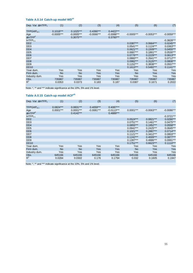
55

Table A.0.14 Catch-up model WDvc

Dep. Var: 𝚫𝚫lnTFPit (1) (2) (3) (4) (5) (6) (7) TFPGAPijt-1 0.1018*** 0.1025*** 0.4390*** 0.4422*** Age -0.0005*** -0.0005*** -0.0066*** -0.0088*** -0.0005*** -0.0053*** -0.0059*** 𝚫𝚫lnTFPF 0.3075*** 0.3760*** lnTFPit-1 -0.3828*** DD2 0.0387*** 0.0664*** 0.0245*** DD3 0.0541*** 0.1124*** 0.0363*** DD4 0.0621*** 0.1509*** 0.0455*** DD5 0.0687*** 0.1861*** 0.0530*** DD6 0.0776*** 0.2229*** 0.0613*** DD7 0.0860*** 0.2641*** 0.0712*** DD8 0.0982*** 0.3120*** 0.0808*** DD9 0.1152*** 0.3838*** 0.0937*** DD10 0.1613*** 0.5482*** 0.1141*** Year dum. Yes Yes Yes Yes Yes Yes Yes Firm dum. No No Yes Yes No Yes Yes Industry dum. Yes Yes Yes Yes Yes Yes Yes Obs. 735987 735987 735987 735987 735987 735987 735987 R2 0.0353 0.0373 0.183 0.187 0.0387 0.1671 0.2022 Note: *, ** and *** indicate significance at the 10%, 5% and 1% level. Table A.0.15 Catch-up model ACFvh

Dep. Var: 𝚫𝚫lnTFPit (1) (2) (3) (4) (5) (6) (7) TFPGAPijt-1 0.0824*** 0.0831*** 0.4059*** 0.4087*** Age 0.0001*** 0.0001*** -0.0081*** -0.0113*** 0.0001*** -0.0063*** -0.0086*** 𝚫𝚫lnTFPF 0.4142*** 0.4889*** lnTFPit-1 -0.3721*** DD2 0.0524*** 0.0821*** 0.0290*** DD3 0.0751*** 0.1461*** 0.0475*** DD4 0.0855*** 0.1952*** 0.0558*** DD5 0.0942*** 0.2425*** 0.0645*** DD6 0.1021*** 0.2887*** 0.0714*** DD7 0.1121*** 0.3412*** 0.0803*** DD8 0.1242*** 0.4009*** 0.0877*** DD9 0.1397*** 0.4886*** 0.0991*** DD10 0.1751*** 0.6623*** 0.1110*** Year dum. Yes Yes Yes Yes Yes Yes Yes Firm dum. No No Yes Yes No Yes Yes Industry dum. Yes Yes Yes Yes Yes Yes Yes Obs. 645166 645166 645166 645166 645166 645166 645166 R2 0.0284 0.0302 0.176 0.1794 0.032 0.1605 0.1947 Note: *, ** and *** indicate significance at the 10%, 5% and 1% level.

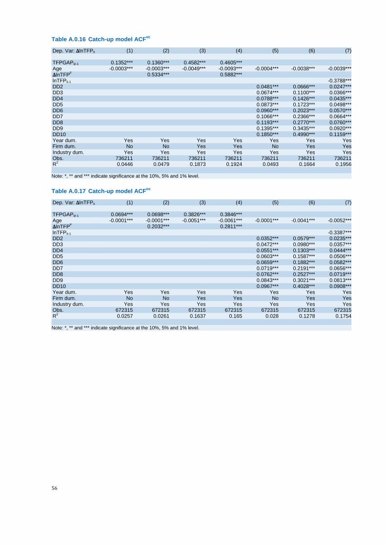
56

Table A.0.16 Catch-up model ACFvc

Dep. Var: 𝚫𝚫lnTFPit (1) (2) (3) (4) (5) (6) (7) TFPGAPijt-1 0.1352*** 0.1360*** 0.4582*** 0.4605*** Age -0.0003*** -0.0003*** -0.0049*** -0.0093*** -0.0004*** -0.0038*** -0.0039*** 𝚫𝚫lnTFPF 0.5334*** 0.5882*** lnTFPit-1 -0.3788*** DD2 0.0481*** 0.0666*** 0.0247*** DD3 0.0674*** 0.1100*** 0.0366*** DD4 0.0788*** 0.1426*** 0.0435*** DD5 0.0873*** 0.1723*** 0.0498*** DD6 0.0960*** 0.2023*** 0.0570*** DD7 0.1066*** 0.2366*** 0.0664*** DD8 0.1193*** 0.2770*** 0.0760*** DD9 0.1395*** 0.3435*** 0.0920*** DD10 0.1850*** 0.4990*** 0.1159*** Year dum. Yes Yes Yes Yes Yes Yes Yes Firm dum. No No Yes Yes No Yes Yes Industry dum. Yes Yes Yes Yes Yes Yes Yes Obs. 736211 736211 736211 736211 736211 736211 736211 R2 0.0446 0.0479 0.1873 0.1924 0.0493 0.1664 0.1956 Note: *, ** and *** indicate significance at the 10%, 5% and 1% level. Table A.0.17 Catch-up model ACFoc

Dep. Var: 𝚫𝚫lnTFPit (1) (2) (3) (4) (5) (6) (7) TFPGAPijt-1 0.0694*** 0.0698*** 0.3826*** 0.3846*** Age -0.0001*** -0.0001*** -0.0051*** -0.0061*** -0.0001*** -0.0041*** -0.0052*** 𝚫𝚫lnTFPF 0.2032*** 0.2811*** lnTFPit-1 -0.3387*** DD2 0.0352*** 0.0579*** 0.0235*** DD3 0.0472*** 0.0980*** 0.0357*** DD4 0.0551*** 0.1303*** 0.0444*** DD5 0.0603*** 0.1587*** 0.0506*** DD6 0.0659*** 0.1882*** 0.0582*** DD7 0.0719*** 0.2191*** 0.0656*** DD8 0.0762*** 0.2527*** 0.0719*** DD9 0.0843*** 0.3021*** 0.0813*** DD10 0.0967*** 0.4028*** 0.0908*** Year dum. Yes Yes Yes Yes Yes Yes Yes Firm dum. No No Yes Yes No Yes Yes Industry dum. Yes Yes Yes Yes Yes Yes Yes Obs. 672315 672315 672315 672315 672315 672315 672315 R2 0.0257 0.0261 0.1637 0.165 0.028 0.1278 0.1754 Note: *, ** and *** indicate significance at the 10%, 5% and 1% level.

Publisher:

CPB Netherlands Bureau for Economic Policy AnalysisP.O. Box 80510 | 2508 GM The Haguet +31 88 984 60 00

info@cpb.nl | www.cpb.nl

July 2018