327

J. Physiol. (949) I09, 327-342 62.816. I

SPACE DISTRIBUTION OF EXCITABILITY IN THE FROG'SSCIATIC NERVE STIMULATED BY SLOT ELECTRODES

BY C. RASHBASS AND W. A. H. RUSHTON

From the Physiological Laboratory, University of Cambridge

(Received 10 October 1948)

The foregoing paper reached the conclusion that when a nerve is excited byslot electrodes, the impulse arises, not at the cathode, but 2 or 3 mm. away onthe cathodal side. Fig. 2 (a) of that paper showed a curve representing thedistribution of excitability about the electrodes which may be called the 'slotexcitability curve ',. but the form was largely conjectural. The only point clearlyestablished was that the maximum of the curve was some 3 mm. distant fromthe manifest cathode. The first object of this paper is to determine experi-mentally the whole slot excitability curve, and the second, to apply; the curveso obtained to predict verifiable excitability results. In Parts I and II twodifferent methods are described by which the slot excitability curve may befound, each strengthening some weak points in the other. In Part III theresults are used to predict both the threshold and the latency of each point onthe family of curves partly shown in Fig. 8 of the previous paper.

It is of course impossible to derive any of these conclusions from excitabilitymeasurements' alone without assuming some guiding principle in their' inter-pretation. The fact that Pig. 6 of the previous Ipaper shows a linear relation atall seems to justify the'ass'umption that excitability (=reciprocal threshold) ata point is an additive quantity. This assumption, which has been accepted bymost' workers in the past, forms the basis of the present analysis.For the sake of concreteness the principal assumptions will now be set' out

in a form rather more definite and restricted than is necessary to justify theconclusions to be drawn from them. Their suibstantiation or modification willbe postponed till the Discussion section at the end of the paper so that thebearing upon the results and conclusions may be appreciated.

Primre assumptions1. The Superposition Theorem holds everywhere in the' nerve structure.

This theorem, which is a generalization of Ohm's Law, applies to'all 'classical'circuits., In the present context it means that if a certain potential distribution

C. RASHBASS AND W. A. H. RUSHTONV1 over the nerve surface produces a potential v, at some given point in thenerve structure (e.g. the membrane depolarization at some point), and if anotherdistribution V2 produces v2 at the same point, then the distribution (V1+ V2)over the surface will produce the sum (vl +v2) at the point.

2. A current pulse of fixed duration will excite a given point in a nerve if,and only if, the membrane depolarization at that point attains a critical thres-hold value. (This threshold usually varies somewhat from point to point alongthe nerve, and also changes with time, etc. The conditions are arranged to be asuniform as possible.)

It may now be stated more precisely what is meant in this paper by 'excita-bility' in a uniform nerve. Suppose v, is the critical membrane depolarizationrequired to excite any point-Assumption (2). Then if a given stimulus Iproduces a depolarization vX at the point x, the local excitability at x is definedas vjlvf

It follows from Assumption (1) that the same stimulus increased to I(vlIvx)brings the depolarization at x exactly to v, and therefore this point is justexcited.

In practice one is concerned with threshold excitation of the whole nerve,i.e. threshold for that point which is most easily excited in the given conditions.Thus the local excitability at x is vxlvc and the whole nerve excitability is vmIvc,where m is the value of x where vx is maximal.

PART I. SLOT EXCITABILITY CURVE

Determination by incrementsPrinciple. It is required to find the excitability produced by a slot electrode

at points on the nerve various distances away from it. What is measured is theexcitability of the whole nerve, and the difficulty is to know exactly where theexcitation is occurring, for unless one is sure of this point one cannot knowwhat distance from the slot corresponds to the threshold reading.

This difficulty may be overcome by the arrangement of Fig. 1. If the nerveis excited at threshold by the slot X alone (Fig. 1 a), with the cathode towards Y,the impulse will arise from a fixed poat P, some 3 mm. to the left of X. Nowif a very small stimulus is simultaneously applied through slot Y (say I/nthreshold where 1/n eventually becomes zero) it will not appreciably changethe locus of excitation, but it will contribute to the excitability an amountwhich can be measured by observing what change is required in the strengthof X, so that the excitation is once more exactly threshold. But the contribu-tion which Y makes to the excitability at P depends directly upon the slotexcitability curve of Y and in this way the curve may be determined. In fact,all that is necessary is to plot a little of the curve relating stimulus X to Y asin Fig. 8 of the previous paper, namely the portion of each curve near B. Then

328

SLOT EXCITABILITY DISTRIBUTION IN NERVEfrom the gradient of each curve at B the ordinate of the required slot excita-bility curve may be at once obtained simply by taking its reciprocal.The truth of this follows readily from Fig. 1 (b). Let the curve XX be the slot

excitability curve due to threshold current at slot X alone, and YY due to Yalone. Then YY will be simply XX laterally displaced by a distance equal tothe slot aeparation. If stimulus Y is l/n threshold, YY must be scaled down toI/n the vertical dimensions (shown dotted). Now the contribution of this 1/nthreshold stimulus AY is obtained by summing XX and the dotted curveYYln. The maximum will still occur at the point P, but the ordinate will be

(a)

Y P ~~X

(b)

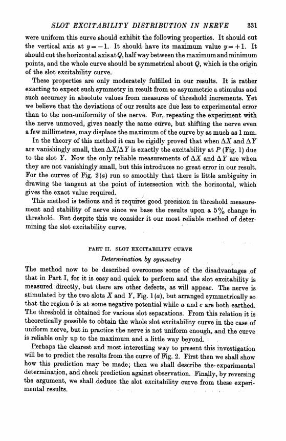
Fig. 1. (a) Arrangement for stimulating nerve by two slots X and Y. (b) Curve XX representsthe space distribution of excitability due to slot X alone; YY due to slot Y.

decreased by y/n, where y is the ordinate of YY at the point P. Similarly, if thestimulus AY were reversed, the maximum would still be at P, but the excita-bility would be increased by the increment y/n. In our experiment, the thres-hold is kept constant by making a small change AX in X to neutralize theeffect of A Y. We have just seen that the magnitude of AX is y/n if AY= 1/nhence AY 1

AX yIn the previous paper, when d-iscussing Fig. 8, the significance-of the different

slopes of the curves at B was pointed out. The present investigation uses thisdeliberately in order to determine exactly the slot excitability curve. For itnow appears that the gradient of the experimental curve at B is the reciprocalordinate of the slot excitability curve for abscissa distance YP. By a morerigid mathematical treatment it may be shown that the very small shift whichoccurs in the locus of the maximum does not affect this result, which is. exactto the first order of infinitesimals.

;329

330 C. RASHBASS AND W. A. H. RUSHTON

Experiment. The frog's sciatic nerve was dissected out and set up in the manner described inPart I of the previous paper. The nerve was placed so that the fixed electrode X lay towards theperipheral end of the uniform thigh region, and the other electrode was moved to various pointscentral to this. 'Threshold' excitation was either half maximal or some smaller fraction of themaximal action potential.The relation between the stimuli X and AY was plotted directly on to paper by the recording

cylinder described in the previous paper. In a preliminary physical calibration we determined theaxees corresponding stimulus X =0, and Y =0, and also the line X = Y which gives the relativescales on the two axes.The actual experiment consisted in plotting the relation between stimulus X and- Y for the

region where the curve cuts the X axis to the right of the origin (i.e. when stimulus X has thepolarity shown in Fig. 1). The experiment is repeated for various positions of the movable slot Y.

(a)O//p 9 <~~~~\_12 14 168 1l

(b) /Q ; w ~~~10mm.

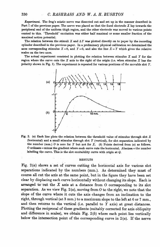
Fig. 2. (a) Each line plots the relation between the threshold value of stimulus through slot X(horizontal) and a small stimulus through slot Y (vertical), for slot separation indicated bythe number (mm.) 0 is zero for Y but not for X. (b) Points derived from (a) as follows.0 ordinate =minus the gradient where ea4h curve 'cuts the horizontal. Abscissa =the numberlabelling the curve. This is the slot excitability curve with origin at Q.

RESULTS

Fig. 2(a) shows a set of curves cutting the horizontal axis for various slotseparations indicated by the numbers (mm.). As determined they must ofcourse all cut the axis at the same point, but in the figure they have been setclear by displacing each curve horizontally without changing its slope. Each isarranged to-'cut the X axis at a distance from 0 corresponding to its slotseparation. As we view Fig. 2 (a), moving from 0 to the right, we note that theslope of the curve where it cuts the axis changes from an inclination to theright, through vertical (at 3 mm.) to a maximum slope to the left at 6 or 7 mm.,and, then returns to the vertical (i.e. parallel to Y axis) at great distances.Plotting the reciprocal of these gradients (suitably corrected for axis obliquityand difference in scales), we obtain Fig. 2(b) where each point lies verticallybelow the intersection point of the corresponding curve in 2 (a). If the nerve

SLOT EXCITABILITY DISTRIBUTION IN NERVEwere uniform this curve should exhibit the following properties. It should cutthe vertical axis at y= -1. It should have its maximum value y= + 1. Itshould cut the horizontal axis at Q, halfwaybetween the maximumandminimumpoints, and the whole curve should be symmetrical about Q, which is the originof the slot excitability curve.

These properties are only moderately fulfilled in our results. It is ratherexacting to expect such symmetry in result from so, asymmetric a stimulus andsuch accuracy in absolute values from measures of threshold increments. Yetwe believe that the deviations of our results are due less to experimental errorthan to the non-uniformity of the nerve. For, repeating the experiment withthe nerve unmoved, gives nearly the same curve, but shifting the nerve evena few millimetres, may displace the maximum of the curve by as much as 1 mm.

In the theory of this method it can be rigidly proved that when AX and AYare vanishingly small, then AX/AY is exactly the excitability at P (Fig. 1) dueto the slot Y. Now the only reliable measurements of AX and A Y are whenthey are not vanishingly small, but this introduces no great error in our result.For the curves of Fig. 2(a) run so smoothly that there is little ambiguity indrawing the tangent at the point of intersection with the horizontal, whichgives the exact value required.

This method is tedious and it requires good precision in threshold measure-ment and stability of nerve since we base the results upon a 5% change inthreshold. But despite this we consider it our most reliable method of deter-mining the slot excitability curve.

PART II. SLOT EXCITABILITY CURVE

Determination by symmetryThe method now to be described overcomes some of the disadvantages ofthat in Part I, for it is easy and quick to perform and the slot excitability ismeasured directly, but there are other defects, as will appear. The nerve isstimulated by the two slots X and Y, Fig. 1 (a), but arranged symmetrically sothat the region b is at some negative potential while a and c are both earthed.The threshold is obtained for various slot separations. From this relation it istheoretically possible to obtain the whole slot excitability curve in the case ofuniform nerve, but in practice the nerve is not uniform enough, and the curveis reliable only up to the maximum and a little way beyond.

Perhaps the clearest and most interesting way to present this investigationwill be to predict the results from the curve of Fig. 2. First then we shall showhow this prediction may be made, then we shall describe theeexperimentaldetermination, and .check prediction against observation. Finally, by reversingthe argument, we shall deduce the slot excitability curve from these experi-mental results.

331

332 C. RASHBASS AND W. A. H. RUSHTONPrediction. Our problem is this. If we know the slot excitability curve and

assume the nerve uniform, what will be the threshold for symmetrical stimula-tion with any slot separation and at which point on the nerve will excitationarise? In principle a method of solution is obvious enough. We may draw theslot excitability curve in two positions, one for each slot. The summed ordinatesgive the resulting excitability for each point on the nerve. Excitation willoccur at the point of maximum excitability and threshold will be the reciprocalof this maximum ordinate. But if a new curve must be plotted for each slotseparation, the process will be rather tedious. The following method is quickerand more illuminating:The slot excitability curve is given by OAB, Fig. 3. Trace this curve on a piece

of card and cut it out together with a portion of the axis OX. Turn the card in its

. .--%

0 X Distance

Fig. 3. Construction for predicting the results of symmetrical stimulation with two slots, when theslot excitability curve is given (see text).

own plane through exactly 180° so that OXj is again horizontal and place it totoucb the curve 0AB at (say) P. Then it will be shown that the co-ordinates of01 give slot separation and the corresponding whole nerve excitability, whilethe co-ordinates of P give the distance from the fixed electrode at whichexcitation arises, and the contribution of this electrode towards the totalexcitability. Clearly, by sliding the card round the curve OAB, the requiredinformation is instantly given for every value of the slot separation.The truth of the above interpretation of the figure will be evident upon

examination, for the meaning of the curve OAB is that the ordinate representsthe excitability at each point due to the fixed slot at 0. Clearly a second slotat a distance from 0 equal to the abscissa of 01 will produce the excitabilityshown upside down by the curve 01A,B1. At the point P the sum of the excita-bilities due to the two slots is equal to the ordinate of 01. At every other pointthe sum of the two excitabilities is less than this by an amount equal to thegap between the two curves. Consequently, P is the point excited at thresholdand the whole nerve excitability is the ordinate of O1.

SLOT EXCITABILITY DISTRIBUTION IN NERVEThis establishes all the features of the foregoing interpretation without any

reference to the fact that OAB and O1A1B1 are the same curve. The constructionis thus seen to be applicable also in the more complicated cases of asymmetricalslots, with which we are not here concerned.

Let us now consider the way in which the card slides over the curve OAB.So long as P lies near the maximum of OAB the curves will be in contact at onepoint only, and this from symmetry must be the mid-point of the line 001.As the curve moves far to the right a new state of affairs arises as shown by theinterrupted curve 02A2B2. The mid-point between the electrodes 0 and 02 ishere less -excitable than regions A2, B2 on either side of it, and excitation willarise from one or other of the two contact points, which are seen to lie near themaximum point of each curve.

It is important to know over what range there is only one contact point, andwhere there are two. This is best found empirically by sliding round the card.It turns out that there is only one contact point P as this slides round from 0up to the maximum and for some way down the right side of the curve. Butat the point of inflexion (where the curve changes from convex upwards toconcave) the contact point becomes double. It is conceivable that the contactpoint might become double before reaching the inflexion point, by the tail ofeach curve hitting the summit of the other, but in practice the curves are notquite the shape to do this.The answer to our problem then is this. The required excitability curve is

given by the (dotted) path traced by 01. This is exactly a reproduction of curveOAB (at magnification x 2) so long as there is a single contact point, and thesite of excitation at threshold will, in this range, be half way between theelectrodes. But as soon as the inflexion point is reached there are two sitespossible for excitation and these rapidly separate to remain close to themaximum point for each slot electrode. From now on, the excitability will benearly the sum of the maximum of one curve and the tail of the other. We turnto the experiment.Apparatus. This was the same as in Part I. The potentials of regions a and c (Fig. 1) were made

the same by earthing both the corresponding silver boxes, and it was verified that electric probesin the two solutions then registered no potential difference. Thresholds were measured by a potentio-meter calibrated against a precision instrument. The only new feature was the measurement of theshock-spike interval. This turned out to be surprisingly accurate and rapid and was done as-follows:A small glass rod had one side ground rough, and it was then drawn out so that it tapered down

to 0-2 mm. in a total length of 10 cm. The roughness was not obliterated by this process so thatwhen a light was shone into the wide end of the rod, some was emitted all the way down instead ofbeing entirely confined. Viewed from the side, therefore, the rod illumined by a 2 V. flash-lampappeared as a fine yellow luminous line. It was mounted vertically just in front of the cathode-raytube (whose time-base was horizontal) in such a way that the line could be set in any desired positionacross the face of the tube and the setting read upon a scale illumined by the same lamp (screenedfrom the front). The green double beam tube was set so that the amplified action potential wasapplied equally to both deflectors. This resulted in the two beams giving mirror-image records,which were arranged so that the monophasic waves approached each other. If the two base-lines

333

334 C. RASHBASS AND W. A. H. RUSHTONwere separated, by a distance equal to the excursion of the maximum action potential, clearly thehalf maximal action potential is given by the conditions where the two reflected waves just touch.This is'a very good index to obs'erve, sinee tho beam becomes twice as bright when the two thinlines overlap. Often 0-2 maximum action potential (or some other small value) was taken, byobserving the coincidence of the mirror peaks when the base-lines were separated by some fractionof the maximal excursion.The vertical yellow line could be set to an accuracy of 1 mm. upon the coincident green peaks

of each 'threshold' setting, and this at a sweep velocity of some 25 mm./msee. means that thepoint of excitation on the nerve could also be localized.correct to 1 mm. It is doubtful, however,whether all the processes contributing to the shock-spike interval remained constant to 0-04 msee.and the inferred excitation sites often exhibited an apparent fluctuation of 1 mm. or so.

Experiment. The nerve was dissected out and set up as before. As far as possible the mostuniform stretch of nerve was selected for the site' of excitation. This was found electrically bydetermining the threshold with a slot separation of 1 mm., as the nerve was gradually drawnthrough the slots by the rack and pinion mechanism. The most uniform region turned out to be thebranch-free stretch in the thigh; other parts unfortunately had a lower threshold and thereforestole the site of excitation when slot separations were large.The experiment was usually performed as follows. At an electrode'separation of. 1 mm. the

threshold and latency were determined. Then the slot separation was increased by 1 mm. and atthe same time the nerve shifted through the slots 0-5 mm. so that the same point, on the nervealways lay midway between the electrodes. Thresholds and latency were again measured. In thisway the double relation was obtained for a wide range ofseparations. Readings were now repeated inreverse sequence. Ifthe two sets agreed closely the average was taken, otherwise they wbre rejected.

In order to be able to convert the observed latency differences into shift of excitation site,conduction velocity of the nerve was found, using only one slot and obtaining the linear relationbetween its setting and the resulting latency. In some experiments (e.g. Fig. 5) the nerve remainedfixed, so the expected excitation site shifted along the nerve.

RESULTS

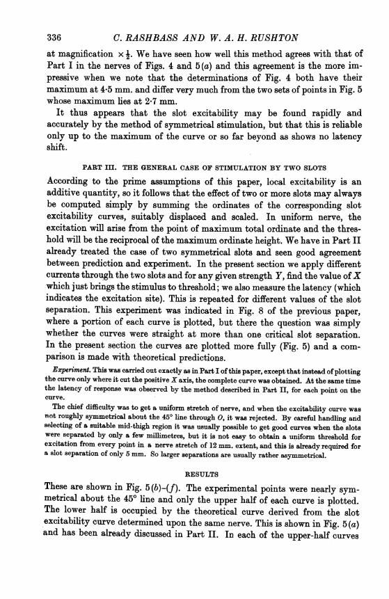
Fig. 4 shows the effect of performing this experiment upon the nerve whichwas used in obtaining Fig. 2. The upper set of points, L, represents the latenciesfound when the stimulus was half-maximal at slot separations. shown by thehorizontal scale. Latencies are converted into distance of propagation, as shownby the scale on the left whose zero is fitted to. the left-hand points. The middleset of points, A, represents the excitability measurements in this experiment.The lower points, B, are those of Fig. 2 .but plotted with origin at Q and scaledso that the maximum height is just half the maximum of A.The curve of B is drawn freehand to fit the points as' in Fig. 2. The curve A

is constructed from B according to the method of Fig. 3. It is exactly the sameas B but at magnification x 2 for a distance 7 x 2 mm. and thereafter lies aboveit. The construction of Fig. 3 also predicts the excitation site, from the contactpoint P. As we have seen, so long as contact is single, the -excitation point willbe midway between the slots. In our experiment the nerve was always adjustedso that this corresponded to the same point on the nerve. The predicted latencyvariation is therefore zero over this range, as shown by the curve L. Beyondthe point of inflexion, however, two contact points appear and rapidly diverge,so. alternative sites are possible as shown by.the two branc4es of L.

SLOT EXCITABILITY DISTRIBUTION IN NERVE

Now, comparing prediction with observation, we see that up to 10 mm.separation the excitability is exact, and the latency shows only two points ofdeviation. For greater distances the excitability is always too high and thelatency mostly too long even for the more delayed branch of L. This is con-sistent with the initial observation that the nerve in the region of the cutbranch to the hamstrings has a decidedly lower threshold than in the moreuniform mid-thigh region. As the slot Y approaches this excitable region,therefore, the excitability will appear higher than predicted, and the latencygreater.

mm

5c . L

-5--10 _

S~~ ~~~~~~~~~ Ai

Q 10 mm. 20

Fig. 4. Curve B with points is a replot of Fig. 2 (b). Curves A and L are predicted from B. by themethod of Fig. 3. Points A and L are re,spectively the observed excitabilities and latencies insymmetrical stimulation. Latency is converted into excitation site by the vertical scale (mm.).

A similar set of determinations upon another nerve is given in Fig. 5(a).For present considerations the continuous line is to be neglected. The dots areobtained by the method of increments as in Fig. 2, the crosses by symmetricalstimulation as in A, Fig. 4, but plotted at half scale. It is seen that here againthe coincidence is good up to, and somewhat past, the maximum.

In this experiment the nerve remained still, hence the predicted latencycurve L will appear plotted upon a slope. The observations are in two sets, leftto right and then right to left. They fit the predictions a little better than inFig. 4.

Determination of the slot excitability curveBy the construction of Fig. 3 we have shown that in uniform nerve, the

excitability curve for symmetrical stimulation is necessarily the same as theslot excitability curve (at magnification x 2) up to some way past the maximumpoint. If we may argue conversely, the required slot excitability curve may beobtained in this range simply by plotting the results of symmetrical stimulation

335

C. RASHBASS AND W. A. H. RUSHTONat magnification x i. We have seen how well this method agrees with that ofPart I in the nerves of Figs. 4 and 5(a) and this agreement is the more im-pressive when we note that the determinations of Fig. 4 both have theirmaximum at 4-5 mm. and differ very much from the two sets of points in Fig. 5whose maximum lies at 2-7 mm.

It thus appears that the slot excitability may be found rapidly andaccurately by the method of symmetrical stimulation, but that this is reliableonly up to the maximum of the curve or so far beyond as shows no latencyshift.

PART III. THE GENERAL CASE OF STIMULATION BY TWO SLOTS

According to the prime assumptions of this paper, local excitability is anadditive quantity, so it follows that the effect of two or more slots may alwaysbe computed simply by summing the ordinates of the corresponding slotexcitability curves, suitably displaced and scaled. In uniform nerve, theexcitation will arise from the point of maximum total ordinate and the thres-hold will be the reciprocal of the maximum ordinate height. We have in Part IIalready treated the case of two symmetrical slots and seen good agreementbetween prediction and experiment. In the present section we apply differentcurrents through the two slots and for any given strength Y, find the value ofXwhich just brings the stimulus to threshold; we also measure the latency (whichindicates the excitation site). This is repeated for different values of the slotseparation. This experiment was indicated in Fig. 8 of the previous paper,where a portion of each curve is plotted, but there the question was simplywhether the curves were straight at more than one critical slot separation.In the present section the curves are plotted more fully (Fig. 5) and a com-parison is made with theoretical predictions.Experiment. This was carried out exactly as in Part I of this paper, except that instead ofplotting

the curve only where it cut the positive X axis, the complete curve was obtained. At the same timethe latency of response was observed by the method described in Part II, for each point on thecurve.The chief difficulty was to get a uniform stretch of nerve, and when the excitability curve was

not roughly symmetrical about the 450 line through 0, it was rejected. By careful handling andselecting of a suitable mid-thigh region it was usually possible to get good curves when the slotswere separated by only a few millimetres, but it is not easy to obtain a uniform threshold forexcitation from every point in a nerve stretch of 12 mm. extent, and this is already required fora slot separation of only 5 mm. So larger separations are usually rather asymmetrical.

RESULTS

These are shown in Fig. 5(b)-(f). The experimental points were nearly sym-metrical about the 450 line and only the upper half of each curve is plotted.The lower half is occupied by the theoretical curve derived from the slotexcitability curve determined upon the same nerve. This is shown in Fig. 5 (a)and has been already discussed in Part II. In each of the upper-half curves

336

SLOT EXCITABILITY DISTRIBUTION IN NERVE(b-f) the circles represent the experimental points and show the relationbetween the stimuli X and Y. The numbers are derived from latency measure-ments as follows. From the measured conduction velocity the observed latencyis converted into propagation distance. Now we have seen (Part II) that insymmetrical stimulation, the excitation site is usually midway between slots.This is the condition where the curves b, c, d, e cut the 450 line. All other pointsare found to have a propagation distance less than this and the difference(shown in millimetres by the numbers on the curve) is therefore the distanceof the excitation site from the mid-point between the slots.

Calculation. In principle this is easy enough, as we have seen, but the work ofscaling and summing two curves for every point to be determined is very heavy.We shall therefore introduce a method less tedious to perform and more instruc-tive to use. In the previous paper it was argued that ifthe relation betweenX andY was linear, then the excitation site was at a fixed point on the nerve. Here weargue the converse, namely that for any fixed point on the nerve to be justexcited requires that the stimuli X and Y should lie on a determined straightline. This follows at once from Fig. 1 (b) where the curves XX, YY represent theslot excitability curves due to unit current at the two slots. Consider theexcitability at some point Q, and let q, r be the ordinates here of the curvesXX, Y Y. It is clear that unit current at slot X produces an excitability q,hence a current x will produce excitability qx. The excitability produced at Qby currents x and y in the two slots will thus be (qx + ry), and if this excitabilityis to remain threshold at Q we have the linear relation

qx + ry= constant.If the nerve is uniform, the constant is the same for all points. It simply altersthe magnification of the figure and may be made unity. Hence the conditionfor excitation at any point Q is exactly determined by the two ordinates at Q,namely q and r (Fig. 1). The result is that X plotted against Y is the straightline which cuts the axes X, Y at the points l/q, I/r respectively.

It is clear then that if we know the slot excitability curve, we may plot ittwice, displaced as in Fig. 1 according to the electrode separation, and for anypoint Q chosen, draw upon the XY excitability diagram, the line

qx+ ry=1

which corresponds to, threshold excitation at Q. The distance of Q from thepoint midway between the slots is known and hence the line may be labelledwith this number of millimetres, thereby defining the excitation site.

In Fig. 5 the slot excitability is shown in (a), and the lower half of the othercurves are determined from it by this method. Now the threshold for thewhole nerve is always given by that portion of line which is first encounteredwhen travelling straight from 0 in any direction. The threshold curve experi-mentally obtained should therefore be the envelope of the family of lines. Of the

337

338 C. RASHBASS AND W. A. H. RUSHTON

1-11 I (C) ' uT) \

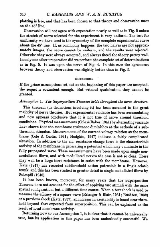
Fig. 5. (a) Slot excitability curve determined by increments (dots) and by symmetry (crosses).Curve L, expected latency, together with observed points. (b) (f) Results of stimulating withtwo slotsX and Y separated by 1, 2, 4, 6, 9 mm. respectively. In each figure current throughXis plotted against Y for threshold. Each threshold point has a number indicating the responselatency. This has been converted into excitation site measured from the point midway betweenthe slots. The experimental results were symmetrical about the 450 line and only the upperhalf is shown. Below the line are the results deduced from the slot excitability curve drawnin (a). The envelope and numbers should be a reflexion in the 450 line of the observed results.

SLOT EXCITABILITY DISTRIBUTION IN NERVE

various kinds of non-uniformity in the nerve which invalidate our results, themost serious is the variation in threshold from point to point. This is a variationin the constant of the linear equation. The method of envelopes shows at oncehow this will affect the curve, for if a given point has an abnormally highthreshold the direction of the corresponding line will be unchanged, but the linewill recede from 0, and will soon be masked by the superior excitability of theneighbours. For this reason, in comparing calculation with observation, rathermore weight should be placed on the slope of the curve at a given number, thanupon its distance from 0.

Comparison between theory and observationThe actual curve used to obtain all the straight lines in Fig. 5 is the continuous

line in Fig. 5 (a). This line was chosen rather than the curve exactly through thepoints, because it gave a distinctly better fit to the curves (b)-(f ) and did notdeviate from the experimental points more than usually happens when theregion of the nerve investigated shifts a little, though it must be admitted thatthe two methods of obtaining the experimental points do not show so muchdeviation. It is clear that the theoretical curves for 1, 2 and 4 mm. are in closeagreement with observation both as to threshold and excitation site. The curvefor 6 mm. corresponds to Fig. 6 of the previous paper. The theoretical curve isalmost exactly a triangle, each side corresponding to a region of constantlatency. The experimental points correspond well enough, but the region at4 mm. from the mid-point appears to have a raised excitability, so line 4 is toonear the origin, and the corner of the triangle somewhat rounded off.

In (f), the curve for 9 mm., the excitation site is measured as usual from thepoint midway between the slots, though this point is never itself excited atthreshold. The black point is given the value -1l5 mm., and all other pointshave the site calculated in the usual way relative to this. It is seen thatobservation and prediction agree fairly well. In addition to these five curveswe have obtained two others entirely comparable. At 3 mm. the curve isintermediate in form between 2 and 4; at 12 mm. the two slots are practicallyindependent of each other and the results form a square.

In observing the rather good fit of observation with theory over a wholefamily of curves, the question which comes to mind is 'How far is this fit due toingenious mathematical manipulation and the careful selection of results?'In Fig. 5 we have in fact improved the results somewhat by operating upon thecontinuous curve 5(a) which does not lie precisely through the points. Thegrounds for doing so were stated above. But if a smooth curve through thepoints were taken instead, the results would still fit the observations ratherwell. The slot excitability curve being given, there is no latitude whatever in themathematical manipulation. Each family of lines, and hence their envelope, isrigidly determined by the construction described above; only the scale of

PH. CIX. 22

339

C. RASHBASS AND W. A. H. RUSHTONplotting is free, ahd that has been chosen so that theory and observation meeton the 450 line.

Observation will not agree with expectation nearly so well as in Fig. 5 unlessthe stretch of nerve gelected for the experiment is very uniform. The test foruniformity we have used is the symmetry of the complete experimental curveabout the 450 line. If, as commonly happens, the two halves are not approxi-mately images, the nerve cannot be uniform, and the results were rejected.Otherwise they were always accepted, and always fitted the theory pretty well.In only one other preparation did we perform the complete set of determinationsas in Fig. 5. It was upon the nerve of Fig. 4. In this case the agreementbetween theory and observation was slightly better than in Fig. 5.

DISCUSSION

If the prime assumptions set out at the beginning of this paper are accepted,the sequel is consistent enough. But without qualification they cannot begranted.

Assumption 1. The Superposition Theorem holds throuqhout the nerve structure.This theorem (or deductions involving it) has been assumed in the great

majority of nerve theories. But experimental evidence has been accumulatingand now appears conclusive that it is not true of nerve around thresholdconditions. Physical measurements (Cole & Baker, 1941) by alternating currentshave shown that the membrane resistance diminishes at the cathode of a sub-threshold stimulus. Measurements of the current-voltage relation at the mem-brane (Cole & Curtis, 1941; Hodgkin, 1947) indicate a fairly complicatedsituation. In addition to the a.c. resistance change there is the characteristicactivity of the membrane in generating a potential which may culminate in thefully propagated wave. These measurements have been made upon single non-medullated fibres, and with medullated nerves the case is not so clear. Theremay well be a large inert resistance in series with the membrane. However,Katz (1947) has recorded subthreshold action potentials in a frog's sciatictrunk, and this. has been studied in greater detail in single medullated fibres byStampffi (1946).

It has been known, moreover, for many years that the SuperpositionTheorem does not account for the effect of applying two stimuli with the samespatial configuration, but a different time course. When a test shock is used tomeasure the efficacy of a square wave (Erlanger & Blair, 1931; Rushton, 1932)or a previous shock (Katz, 1937), an increase in excitability is found near thres-hold beyond that expected from superposition. This can be explained as theresult of local membrane activity.

Returning now to our Assumption 1, it is clear that it cannot be universallytrue, but its application in this paper has been undoubtedly successful. We

340

SLOT EXCITABILITY DISTRIBUTION IN NERVEneed to be satisfied why it is legitimate to superpose stimuli with the same timecourse but a different space configuration, but not the other way round wherethe electrodes are the same but the time course is varied. The explanation isprobably as follows.The Superposition Theorem holds well enough for anodal currents, and weak

cathodal currents; it is only in the neighbourhood of actual excitation that itbreaks down. Now in all the excitability measurements of this paper we aresimply concerned with threshold excitability at some point due to a stimulus offixed duration, and this requires that the current leaving the nerve axis cylinderat the point should have a fixed value (see Assumption 2, below). A fixedcurrent at the excitation site is thus secured in every measurement; what isvaried is the distribution of the current in the remoter regions. But there thecurrent has the density and polarity which satisfies the Superposition Theorem.Assumption 1 is valid, therefore, in these experiments because they secure thatin the only region where the Superposition Theorem is not valid, the current isinvariant.Though the above explanation may well be correct we are not convinced that it necessarily is so.

In Katz's results(1937) superposition begins to break down when the local excitability exceeds 50%,and in our experiments the space distribution about the cathode changes somewhat as the condi.tions of stimulation are varied. In these circumstances we cannot estimate how far the cathodalconditions may be regarded as invariant, but at present it seems reasonable to accept Assumption 1as applicable to the conditions of our experiment.

Assumption 2. The necessary and sufficient condition for nerve excitation is thatthe stimulating current leaving the sheath at some point should attain a fixedvalue.

Nearly all the excitation theories since Nernst (1899) have assumed thata critical depolarization at some point of the membrane was the necessary- andsufficient condition for excitation. But this is not true for non-medullatednerve, for Hodgkin (1938) showed that the transition from local to propagatedresponse depended in general, not only upon the strength ofstimulating current,but also upon the spatial spread of excitability from the cathode. In the caseof medullated nerve, on the other hand, Tasaki (1939) gives evidence whichgoes some way to prove that a critical depolarization at a single node is thecondition sufficient for propagation. Using tripolar stimulation with electrodesapplied to three adjacent nodes of a single fibre, he obtains results which fallexactly upon a triangle (his Fig. 2). This seems to indicate that the samecurrent is required to excite a single node no matter what (subthreshold)current is applied to the neighbouring nodes. And he draws attention to thefact that his results show excitability to be a strictly additive quantity.

In our paper the conditions of stimulation are far less critical than in eitherHodgkin's or Tasaki's. The slot excitability has a gently rounded maximum, andso in all our experiments the impulse might be expected to arise almost simul-

22-2

341

C. RASHBASS AND W. A. H. RUSHTON'taneously over several millimetres of nerve. This is what in fact was found tooccur in the previous paper, Fig. 10, when the records were led from the actualsite of excitation. Assumption 2 is valid, therefore, in these experiments becausewhen the membrane current at the excitation site has the critical value, it hasnearly the same value for a millimetre or so on either side. Hence the localpotential arises in conditions suitable for its immediate propagation, and wemay neglect the exact locality of the nodes of Ranvier.From this discussion it appears reasonable to accept our prime assumptions

as applicable to the conditions of the experiments of this paper. The wholeanalysis then follows inevitably, and the results are encouraging. It has beenpossible to obtain the slot excitability curve by two very different methods,and to apply the curve so obtained to predict rather accurately the thresholdand latency over the whole range of stimulation with two slots. If we mayextend the method to any number of slots arbitrarily disposed, we shall obtainthe complete solution of the problem of space distribution of excitability.Since, however, it is rather a large step to argue from experiments with two slotsto conclusions about twenty, we shall postpone the general theory until thisstep has been strengthened by the experiments of the two papers which follow.

SUMMARY

1. The paper attempts to determine the spatial distribution of excitabilityin the neighbourhood of a slot electrode-the slot excitability curve.

2. Experimental results are analysed in terms of two prime assumptionsgiven on p. 327 and discussed on p. 340.

3. Two methods are used to determine the curve; they give good agreementover the admissible range, Figs. 4 and 5 (a).

4. If the slot excitability curve is known, it is possible to calculate foruniform nerve the space distribution of excitability for any electrode arrange-ment. Fig. 5 (b)-(f) shows the comparison between prediction and observationover the full range where two slots of varying strength and position are usedsimultaneously to stimulate.

C. Rashbass wishes to thank the Medical Research Council for assisting this work with a Researchtraining grant.

REFERENCESCole, K. S. & Baker, R. F. (1941). J. gen. Phy8iol. 24, 535.Cole, K. S. & Curtis, H. J. (1941). J. gen. Phy8iol. 24, 551.Erlanger, J. & Blair, E. A. (1931). Amer. J. Physiol. 99, 108.Hodgkin, A. L. (1938). Proc. Roy. Soc. B, 126, 87.Hodgkin, A. L. (1947). J. Phy8iol. 106, 305.Katz, B. (1937). Proc. Roy. Soc. B, 124, 244.Katz, B. (1947). J. Phy8iol. 106, 66.Nernst, W. (1899). Nachrichten K. ge8. d. Wi88. zu G6ttingen Math. Phy8. Ki. p. 104.Rushton, W. A. H. (1932). J. Physiol. 75, 16P.Stimpfli, R. (1946). Helvetica Phy8iol. et Pharm. Acta, 4, 417.Tasaki, I. (1939). Amer. J. Phy8iol. 125, 367.

342