FROM STRUCTURE TO FUNCTION IN PROTEINS: A …

FROM STRUCTURE TO FUNCTION IN

PROTEINS: A COMPUTATIONAL STUDY

A thesis submitted to the University of Manchester for the degree of

Doctor of Philosophy in the Faculty of Life Sciences

2010

Tracey Bray

Faculty of Life Sciences

2

List of Contents ABSTRACT ............................................................................................................................................. 14

DECLARATION ..................................................................................................................................... 15

COPYRIGHT .......................................................................................................................................... 16

ACKNOWLEDGEMENTS .................................................................................................................... 17

THE AUTHOR ........................................................................................................................................ 18

CHAPTER 1: INTRODUCTION....................................................................................................... 19

1.1 PROTEINS AND THEIR ROLE IN BIOLOGY ....................................................................................... 19

1.1.1 Enzymes ............................................................................................................................. 20

1.1.1.1 Enzyme Kinetics ..........................................................................................................................23

1.1.1.2 Enzyme Functions ........................................................................................................................25

1.2 COMPUTATIONALLY DETERMINING PROTEIN FUNCTION............................................................... 30

1.2.1 Defining Protein Function ................................................................................................. 32

1.2.1.1 Classification Schemes.................................................................................................................32

1.2.2 Functional Transfer Based on Homology.......................................................................... 35

1.2.2.1 Sequence Similarity......................................................................................................................38

1.2.2.2 Structural Similarity .....................................................................................................................39

1.2.2.3 Dynamic Similarity ......................................................................................................................40

1.2.3 Predicting Protein Function in the Absence of Sequence or Structural Similarity............ 41

1.2.3.1 Sequence Motifs...........................................................................................................................41

1.2.3.2 Functional Sites ............................................................................................................................44

1.2.3.3 Genomic Context..........................................................................................................................47

1.2.3.4 Protein-Protein Interactions..........................................................................................................49

1.2.3.5 Subcellular Localisation ...............................................................................................................50

1.2.3.6 Structural Features........................................................................................................................51

1.3 THESIS STRUCTURE...................................................................................................................... 54

1.4 REFERENCES ................................................................................................................................ 55

CHAPTER 2: SEQUENCE AND STRUCTURAL FEATURES OF ENZYMES BY EC CLASS

63

2.1 INTRODUCTION ............................................................................................................................ 63

2.2 METHODS..................................................................................................................................... 66

2.2.1 Dataset Creation................................................................................................................ 66

2.2.2 Defining Active Site Residues ............................................................................................ 67

2.2.3 Calculating Features ......................................................................................................... 68

2.2.4 Culling Redundancy in Features. ...................................................................................... 69

2.2.5 Statistical Analysis............................................................................................................. 69

2.2.6 Rotamer Calculations. ....................................................................................................... 71

2.3 RESULTS AND DISCUSSION........................................................................................................... 72

3

2.3.1 Dataset and Active Site Definition. .................................................................................... 72

2.3.2 Overall Description of Features. ....................................................................................... 76

2.3.3 Unique Descriptive Features. ............................................................................................ 83

2.3.4 Differences in Structure Sizes due to Different Oligomeric State Preferences .................. 86

2.3.4.1 Lyases and Hydrolases in Metabolic Networks............................................................................89

2.3.5 Active-site Non-polarity in Oxidoreductases ..................................................................... 92

2.3.6 Active-site Aspartic Acid Content in Oxidoreductases ...................................................... 94

2.3.6.1 Rotamers ......................................................................................................................................95

2.3.6.2 Hydrogen Bonding .......................................................................................................................96

2.4 CONCLUSIONS .............................................................................................................................. 98

2.5 REFERENCES .............................................................................................................................. 101

CHAPTER 3: FUNCTIONAL SITE IDENTIFICATION IN PROTEINS .................................. 104

3.1 INTRODUCTION: COMPUTATIONAL APPROACHES FOR THE PREDICTION OF FUNCTIONAL SITES .. 105

3.2 METHODS: BENCHMARKING THE ACCURACY OF FUNCTIONAL SITE IDENTIFICATION TOOLS .... 109

3.2.1 Selection of Prediction Methods ...................................................................................... 109

3.2.2 Creation of Test Sets ........................................................................................................ 114

3.2.3 Obtaining and Unifying Functional Site Predictions....................................................... 117

3.3 METHODS: SITESIDENTIFY WEBSERVER .................................................................................... 120

3.3.1 Functional Site Prediction Methods ................................................................................ 120

3.3.2 SitesIdentify Workflow ..................................................................................................... 122

3.3.3 SitesIdentify Usage .......................................................................................................... 122

3.4 RESULTS: BENCHMARKING THE ACCURACY OF FUNCTIONAL SITE IDENTIFICATION TOOLS ...... 124

3.4.1 Recall Accuracy Rates for Real Sites ............................................................................... 124

3.4.2 Crescendo ........................................................................................................................ 126

3.4.3 PASS ................................................................................................................................ 130

3.4.4 Fuzzy Oil Drop ................................................................................................................ 134

3.4.5 QSiteFinder...................................................................................................................... 139

3.4.6 PDBSiteScan.................................................................................................................... 143

3.4.7 Consurf ............................................................................................................................ 147

3.4.8 Thematics......................................................................................................................... 151

3.4.9 SitesIdentify(GM) – Geometry-based............................................................................... 154

3.4.10 SitesIdentify(ConsGM) – Conservation and geometry-based ..................................... 158

3.4.11 All Methods ................................................................................................................. 161

3.5 RESULTS: SITESIDENTIFY WEB-SERVER ..................................................................................... 165

3.6 DISCUSSION ............................................................................................................................... 170

3.7 REFERENCES .............................................................................................................................. 172

CHAPTER 4: PREDICTING EC CLASS FROM ENZYME STRUCTURE.............................. 176

4.1 INTRODUCTION .......................................................................................................................... 176

4.1.1 Machine Learning Theory ............................................................................................... 178

4.1.1.1 Support Vector Machines ...........................................................................................................180

4

4.2 METHODS................................................................................................................................... 186

4.2.1 Dataset Creation.............................................................................................................. 186

4.2.2 Defining Active Site Residues .......................................................................................... 187

4.2.2.1 Dataset 4.1..................................................................................................................................187

4.2.2.2 Dataset 4.2..................................................................................................................................187

4.2.3 Calculating Features. ...................................................................................................... 187

4.2.3.1 Structural Features......................................................................................................................188

4.2.3.2 Sequence Features ......................................................................................................................189

4.2.4 Prediction Methods.......................................................................................................... 190

4.2.4.1 Functional Classification where the Active Site is Known.........................................................190

4.2.4.2 Functional Prediction where the Active Site is not Known ........................................................192

4.3 PREDICTING EC CLASS FOR ENZYMES WITH KNOWN ACTIVE SITE LOCATION .......................... 194

4.4 PREDICTING EC CLASS FOR ENZYMES WITH PREDICTED ACTIVE SITE LOCATIONS.................... 197

4.5 CONCLUSIONS ............................................................................................................................ 202

4.6 REFERENCES .............................................................................................................................. 203

CHAPTER 5: GAUSSIAN NETWORK MODELING OF OLIGOMERIC PROTEINS .......... 205

5.1 INTRODUCTION .......................................................................................................................... 205

5.1.1 Cooperativity in Oligomeric Enzymes ............................................................................. 205

5.1.2 Application of Normal Mode Analysis to the Study of Proteins....................................... 210

5.1.3 Normal Mode Analysis and the Gaussian Network Model .............................................. 213

5.2 METHODS................................................................................................................................... 217

5.2.1 Dataset Creation for the Cooperativity Analysis ............................................................. 217

5.2.2 Dataset Creation for the Active Site Correlation Analysis .............................................. 221

5.2.3 Dataset Creation for the Structural Environment Correlation Analysis ......................... 222

5.2.4 Calculation of Residue Motion Correlation..................................................................... 225

5.3 CORRELATED RESIDUE MOTIONS IN COOPERATIVE OLIGOMERIC ENZYMES ............................. 228

5.3.1 Analysis of Residue Correlations in Co-operative and Non Cooperative Enzymes......... 229

5.3.2 Discussion of Cooperative Enzyme Analysis ................................................................... 238

5.4 CORRELATION OF RESIDUE MOTIONS IN ENZYME ACTIVE SITE REGIONS.................................. 240

5.4.1 Analysis of Residue Correlations in Enzyme Active Sites ................................................ 240

5.4.2 Discussion of Correlation of Motion in Active Sites ........................................................ 245

5.5 PATTERNS OF CORRELATION OF RESIDUE MOTION AS A STRUCTURAL FEATURE OF OLIGOMERIC

PROTEINS............................................................................................................................................. 246

5.5.1 Differences in Residue Motion Correlation According to Structural Environment......... 247

5.5.1.1 Are Residues with High Dynamic Coupling to their Equivalent Residues more Evolutionarily

Conserved?.................................................................................................................................................258

5.5.2 Discussion of Correlation of Motion According to Structural Environment ................... 260

5.6 CONCLUSIONS ............................................................................................................................ 263

5.7 REFERENCES .............................................................................................................................. 266

CHAPTER 6: CONCLUSIONS ....................................................................................................... 272

Final word count : 65,147

5

List of Figures

Figure 1.1 A schematic representation of how an enzyme increases the rate of reaction by

lowering the energy barrier in order for the reaction to proceed. ........................................... 21

Figure 1.2 Schematic illustration of the concerted and sequential models for cooperative

substrate binding............................................................................................................................. 22

Figure 1.3 A simplified representation of a mechanism for single-substrate enzyme

reactions. .......................................................................................................................................... 23

Figure 1.4 A Michaelis-Menton graph showing the maximum velocity at saturation (Vmax),

and the Michaelis-Menton constant (Km).................................................................................... 24

Figure 1.5 A plot showing the difference in change in reaction rate with the concentration

between cooperative and non-cooperative enzymes. ................................................................ 25

Figure 1.6 A simple example of a redox reaction. ..................................................................... 27

Figure 1.7 A simple example of a transferase reaction.............................................................. 27

Figure 1.8 A schematic equation for the hydrolysis reaction. .................................................. 27

Figure 1.9 The proportion of each top EC class in the PDB. ................................................. 29

Figure 1.10 The rise in the number of structures deposited into the PDB since 1986. ....... 31

Figure 1.11 The accuracy of function annotation with varying sequence identity................ 37

Figure 1.12 Schematic diagram of a generic approach for constructing sequence motifs... 42

Figure 1.13 A schematic representation of the Rosetta Stone method of assigning protein

function. ........................................................................................................................................... 48

Figure 1.14 The 52 structural features used to classify into enzyme/non-enzyme from a

previous study by Dobson and Doig .......................................................................................... 53

Figure 2.1 A flow diagram showing how the dataset is culled from the original 880 CSA

literature entries to the dataset of 294 unique non-redundant enzymes................................. 73

Figure 2.2 The percentage coverage of CSA residues by varying active site criteria

thresholds for (a) surface area and (b) distance from centroid. ............................................... 75

Figure 2.3 The median aromatic proportion of the active site for each EC class................. 79

Figure 2.4 Amino acids that showed significant differences between the six EC classes in

either the active site, surface residues or the total protein........................................................ 79

Figure 2.5 The median value of significantly different charge-related features for each EC

class. .................................................................................................................................................. 80

6

Figure 2.6 The median proportion of the total surface area that belongs to the active site

for each EC class. ........................................................................................................................... 80

Figure 2.7 The median value of significantly different size-related features for each EC

class. .................................................................................................................................................. 80

Figure 2.8 The median value of the total sum of B factors for each EC class. ..................... 81

Figure 2.9 The percentage of each EC class on each oligomeric status catergory................ 81

Figure 2.10 The median amino acid composition of the total protein for amino acids

showing significant differences between the EC classes........................................................... 81

Figure 2.11 The median amino acid composition of the protein surface for amino acids

showing significant differences between the EC classes........................................................... 82

Figure 2.12 The median amino acid composition of the active site for amino acids showing

significant differences between the EC classes .......................................................................... 82

Figure 2.13 A network diagram showing the significantly different features (as nodes)

connected by lines where there is a probable correlation (the R value is more than 0.195,

the critical R value at the 5% significance level)......................................................................... 84

Figure 2.14 The median proportion of the total protein that is either helix or non-helix and

non-sheet for each EC class. ......................................................................................................... 85

Figure 2.15 The percentage of oligomers that have single sub-unit or shared sub-unit active

sites in each class............................................................................................................................. 89

Figure 2.16 The observed number of enzymes divided by the expected number of enzymes

in each class for all choke points and the 50% most loaded choke points in the

Saccharomyces cerevisiae metabolic network. .................................................................................... 91

Figure 2.17 The observed number of enzymes divided by the expected number of enzymes

in each class for the 25% most loaded enzymes (incoming and outgoing) from the yeast

metabolic network. ......................................................................................................................... 92

Figure 2.18 The distribution of active site non-polar proportions for the cofactor-binding

and non-cofactor-binding oxidoreductases. ............................................................................... 93

Figure 2.19 The percentage of enzymes in each set that prefer aspartic acid as an active site

residue (there is a higher proportion of active site ASP than GLU), prefer glutamic acid as

an active site residue (there is a higher proportion of active site GLU than ASP), and where

there are equal amounts of aspartic and glutamic acid in the active sites............................... 94

Figure 2.20 The percentage of accessible rotamers available to all active site ASP and GLU

in each class. .................................................................................................................................... 96

Figure 2.21 The underlying distribution for the number of hydrogen bonds per ASP or

GLU in the active site for EC1..................................................................................................... 97

7

Figure 3.1 The asymmetric unit structure of 1daa. .................................................................. 119

Figure 3.2 Distribution of annotated residues recall rates in real sites. ................................ 125

Figure 3.3 The distribution of absolute recall rates per protein for Crescendo in A) the

enzyme set and B)the non-enzyme set. ..................................................................................... 128

Figure 3.4 The cumulative percentage of distances between Crescendo-predicted and real

centroids within the two sets. ..................................................................................................... 129

Figure 3.5 Diagram taken from Brady and Stouten, 2000 showing how the PASS method

defines buried volume.................................................................................................................. 130

Figure 3.6 The distribution of absolute recall rates per protein for PASS in A) the enzyme

set and B) the non-enzyme set.................................................................................................... 132

Figure 3.7 The cumulative percentage of distances between PASS-predicted and real


Figure 3.8 The distribution of absolute recall rates per protein for FOD in A) the enzyme

set and B) the non-enzyme set.................................................................................................... 137

Figure 3.9 The cumulative percentage of distances between FOD-predicted and real


Figure 3.10 The distribution of absolute recall rates per protein for QSiteFinder in A) the

enzyme set and B) the non-enzyme set. .................................................................................... 141

Figure 3.11 The cumulative percentage of distances between QSiteFinder-predicted and

real centroids within the two sets. .............................................................................................. 142

Figure 3.12 The distribution of absolute recall rates per protein for PDBSiteScan in A) the


Figure 3.13 The cumulative percentage of distances between PDBSiteScan-predicted and

real centroids within the two sets. .............................................................................................. 146

Figure 3.14 The distribution of absolute recall rates per protein for Consurf in A) the


Figure 3.15 The cumulative percentage of distances between Consurf-predicted and real


Figure 3.16 The distribution of absolute recall rates per protein for Thematics in the

enzyme set...................................................................................................................................... 152

Figure 3.17 The cumulative percentage of distances between Thematics-predicted and real

centroids within the enzyme set. ................................................................................................ 153

Figure 3.18 The distribution of absolute recall rates per protein for SitesIdentify(GM) in A)

the enzyme set and B) the non-enzyme set. ............................................................................. 156

8

Figure 3.19 The cumulative percentage of distances between SitesIdentify(GM) predicted

and real centroids within the enzyme and non-enzyme set.................................................... 157

Figure 3.20 The distribution of absolute recall rates per protein for SitesIdentify(ConsGM)

in A) the enzyme set and B) the non-enzyme set. ................................................................... 160

Figure 3.21 The cumulative percentage of distances between SitesIdentify(ConsGM)

predicted and real centroids within the enzyme and non-enzyme set. ................................. 161

Figure 3.22 Comparison of distances between the real centroids and the predicted

centroids in the enzyme dataset for each method. .................................................................. 162

Figure 3.23 Comparison of distances between the real centroids and the predicted

centroids in the non-enzyme dataset for each method. .......................................................... 162

Figure 3.24 Comparison of distances between the real centroid and the predicted centroid

for Consurf and SitesIdentify(ConsGM) run on the first chain of the enzyme structures.

......................................................................................................................................................... 164

Figure 3.25 Screenshot for SitesIdentify showing the required user input fields............... 166

Figure 3.26 Screenshot of an example results output for SitesIdentify. .............................. 167

Figure 3.27 An example of highlighted residues in an alternative predicted site. ............... 168

Figure 3.28 An example of differential site prediction between asymmetric and biological

unit structures................................................................................................................................ 169

Figure 4.1 A schematic diagram representing the classification of two groups of data by an

SVM model.................................................................................................................................... 181

Figure 4.2 A schematic diagram representing how the transformation of data into a higher-

dimensional space by using kernel functions can allow the separation of the data by a linear

function. ......................................................................................................................................... 182

Figure 4.3 An example of a decision tree that can be followed to classify into multiple

groups using binary classifications. ............................................................................................ 183

Figure 4.4 A schematic diagram showing how varying the error penalty parameter, C can

identify a hyperplane that achieves a high accuracy on test data. .......................................... 185

Figure 4.5 A schematic representation of the vector comparison method used to predict

the EC class of enzymes with known active sites. ................................................................... 191

Figure 4.6 Accuracies achieved using the top n-ranked features in the prediction model.195

Figure 4.7 Prediction accuracies achieved using a default grid search method for the best C

and γ parameters. A) Shows the accuracies on a 2D plot and B) shows this in 3D.......... 198

Figure 4.8 Accuracies achieved using the top-ranked features with 10-fold cross-validation

on the training set. ........................................................................................................................ 199

9

Figure 5.1 Example reaction rate (v/Vmax) vs. substrate concentration ([S]) for a non-

cooperative (A), a positively cooperative (B) and a negatively cooperate enzyme (C). ...... 207

Figure 5.2 A protein structure (lysine–arginine–ornithine binding protein; top) shown as an

elastic network............................................................................................................................... 214

Figure 5.3 A schematic representation of the basic terms used in the Gaussian network

model. ............................................................................................................................................. 216

Figure 5.4 An example of a protein structure (1ji7) with the interface residues highlighted.

......................................................................................................................................................... 223

Figure 5.5 An example cross-correlation matrix for 1D3V (Manganese Metalloenzyme

Arginase), which is a homo-trimer. ............................................................................................ 226

Figure 5.6 The biological unit structure for 1D3V coloured according to each residue’s

cc_equiv score. .............................................................................................................................. 228

Figure 5.7 Positively cooperative enzyme structures............................................................... 232

Figure 5.8 Negatively cooperative enzyme structures. ............................................................ 233

Figure 5.9 Non-cooperative enzyme structures. ...................................................................... 234

Figure 5.10 Distribution of all residue’s cc_equiv values for positively, negatively and non-

cooperative enzymes. ................................................................................................................... 238

Figure 5.11 The distribution of scaled cc_equiv values for site and non-site residues for all

enzymes in the dataset. ................................................................................................................ 242

Figure 5.12 The cumulative percentage of cc_equiv values for all site and non-site residues

in each set....................................................................................................................................... 242

Figure 5.13 The distribution of scaled cc_equiv scores for each structural environment

over all residues in the dataset. ................................................................................................... 248

Figure 5.14 The distribution of Spearman’s rank correlation coefficients between cc_equiv

values and distance between equivalent residues for individual proteins in the dataset. ... 252

Figure 5.15 An example of a protein in the dataset (1h16) where the closest equivalent

residues in the interface have the highest dynamic coupling and the rest of the interface

residues are less-coupled in comparison. .................................................................................. 253

Figure 5.16 The distribution of scaled cc_equiv values for the closest pair of equivalent

residues in each protein. .............................................................................................................. 254

Figure 5.17 The distribution of scaled distances between the most highly-correlated

equivalent pair in each protein.................................................................................................... 254

Figure 5.18 The distribution of Spearman’s correlation coefficients between cc_within and

cc_equiv values for all proteins in the set. ................................................................................ 255

10


cc_equiv values derived from GNM calculations on both the oligomer and the individual

subunits for all proteins in the set. ............................................................................................. 256

Figure 5.20 An example of a protein (1cq3) with residues coloured by cc_equiv value (A),

cc_within values derived using GNM calculations on the oligomer (B), and cc_within

values derived from GMN calculations on the individual monomers(C). ........................... 257

Figure 5.21 The distribution of Spearman’s correlation coefficients for the relationship

between conservation and degree of correlation of motion between equivalent residues for

each protein in the set. ................................................................................................................. 259

Figure 5.22 The cross-correlation matrix for a homo-trimer (1d3v), which shows obvious

patterns of correlation between residues within subunits but less definition between

residues in different subunits. ..................................................................................................... 262

11

List of Tables Table 1.1 A table showing how the coverage of classification schemes varies per protein. 35

Table 1.2 The main primary sequence databases with their URL and relevant reference. .. 38

Table 1.3 Examples of structure comparison programs with their URL and reference. ..... 39

Table 1.4 A list of sequence motif resources.............................................................................. 43

Table 1.5 Functional/active/binding site residue databases and comparison tools available

via the web. ...................................................................................................................................... 45

Table 2.1 PDB codes for each enzyme in the dataset. .............................................................. 74

Table 2.2 List of all features calculated for each enzyme.......................................................... 77

Table 2.3 The p-value (adjusted for the false discovery rate), the EC class that had the

highest mean or median value and the EC class with the lowest mean or median value for

all features that showed a significant difference between EC classes (p<0.05)..................... 78

Table 2.4 The correlation between total leucine and proline composition and the secondary

structure environments that they are typically associated with. ............................................... 84

Table 2.5 Subcellular location annotation (where available) for each EC class..................... 88

Table 2.6 Number of enzymes that are bound to cofactors and those that are not............. 93

Table 2.7 Average number of hydrogen bonds per aspartic acid/glutamic acid split by

active-site residues and non-active-site residues ........................................................................ 97

Table 3.1 The seven tools used in this analysis along with the broad category of their

method. Each method is described in more detail in their relevant section below. .......... 110

Table 3.2: Functional site prediction tools not included in the comparison analysis.

Reasons for non-inclusion in the analysis are further explained below:............................... 113

Table 3.3 The PDB codes for the 237 structures in the enzyme dataset ............................. 115

Table 3.4 The PDB codes for the 13 structures in the non-enzyme dataset. ...................... 116

Table 3.5 Annotated residues recalled by the site definition criteria..................................... 125

Table 3.6 The functional site prediction accuracy results for Crescendo............................. 127

Table 3.7 The functional site prediction accuracy results for PASS. .................................... 131

Table 3.8 The functional site prediction accuracy results for FOD...................................... 136

Table 3.9 The functional site prediction accuracy results for QSiteFinder.......................... 140

Table 3.10 The functional site prediction accuracy results for PDBSiteScan...................... 144

Table 3.11 The functional site prediction accuracy results for Consurf. .............................. 148

Table 3.12 The functional site prediction accuracy results for Thematics. .......................... 152

Table 3.13 The functional site prediction accuracy results for SitesIdentify (Uniform charge

method) .......................................................................................................................................... 155

12

Table 3.14 The functional site prediction accuracy results for SitesIdentify(ConsGM). ... 159

Table 3.15 The absolute and relative recall rates achieved for the enzyme dataset along with

the average distance between real and predicted centroids for each method...................... 163

Table 3.16 The absolute and relative recall rates achieved for the non-enzyme dataset along

with the average distance between real and predicted centroids for each method. ............ 163

Table 4.1 Features used in the EC class prediction methods................................................. 188

Table 4.2 Features that are removed in the EC class prediction method where the active

site location is known................................................................................................................... 196

Table 4.3 The number of enzyme structures in each class in Dataset 4.2............................ 197

Table 4.4 The 10 lowest ranked features that were removed from the dataset to train the

final model. .................................................................................................................................... 199

Table 4.5 The number of predictions of each class made by the model without class

weightings. ..................................................................................................................................... 200

Table 4.6 The number of predictions of each class made by the model with class

weightings. ..................................................................................................................................... 201

Table 5.1 Dataset 5.1: A list of enzymes with annotated Hill coefficients and a structure

deposited in the PDB for the same organism. ......................................................................... 220

Table 5.2 Dataset 5.2. A list of 114 non redundant homo-oligomeric enzyme PDB

structures with a literature-based active site information obtained from the CSA. ............ 221

Table 5.3 Dataset 5.3: A list of 636 non-redundant homo-oligomeric PDB structures. ... 224

Table 5.4 The average equivalent residue cross-correlation (cc_equiv) scores for site and

non-site residues for cooperative and non-cooperative enzymes.......................................... 235

Table 5.5 The Spearman’s rank correlation coefficient for the comparison between distance

from active site centroid and cc_equiv for each enzyme........................................................ 237

Table 5.6 Average scaled cc_equiv values for pooled residues from enzymes within each

set. ................................................................................................................................................... 237

Table 5.7. Site correlation vs. non-site correlation results for individual enzymes within the

set. ................................................................................................................................................... 241

Table 5.8 The Spearman’s rank correlation coefficient for the relationship between distance

from active site centroid and cc_equiv for all enzymes in the set. ........................................ 243

Table 5.9 Table showing the breakdown of Spearman’s rank correlation coefficients

between distance from active site centroid and cc_equiv value for individual enzymes in

the dataset. ..................................................................................................................................... 243

Table 5.10 The number of proteins in the whole dataset that have either a lower or higher

average active site B-factor than non-site residues, split by significance.............................. 244

13

Table 5.11 The number of proteins in the whole dataset that have either a negative or

positive correlation between B-factor and cc_equiv, split by significance. .......................... 244

Table 5.12 Number of proteins where the active site residues are significantly more

correlated than non-site residues that have either higher or lower average site B-factors in

comparison to the rest of the protein, split by significance. .................................................. 244

Table 5.13 Number of proteins where the active site residues are significantly more

correlated than non-site residues that have either a positive or negative relationship

between cc_equiv and B-factor, split by significance. ............................................................. 244

Table 5.14 The mean scaled cc_equiv values for each structural environment for pooled

residues from all proteins in the set. .......................................................................................... 248

Table 5.15. Pairwise comparison of average cc_equiv values for each structural

environment. ................................................................................................................................. 249

Table 5.16 The number of proteins in the Dataset 2.3 that have either a negative or

positive correlation between B-factor and cc_equiv, split by significance. .......................... 250

Table 5.17 The average scaled B-factors for each structural environment over all residues

in the set. ........................................................................................................................................ 250

Table 5.18 Pairwise comparison of average scaled B-factors for each structural

environment. ................................................................................................................................. 250

Table 5.19 The average scaled distance between equivalent residues for each structural

environment over all residues in the set. ................................................................................... 250

Table 5.20 The number of proteins in the Dataset 2.3 that have either a negative or

positive correlation between the distance between equivalent residues and cc_equiv, split

by significance. .............................................................................................................................. 252

Table 5.21 The average scaled conservation score for each structural environment. ........ 258

List of Equations

Equation 1.1 The Hill equation. ................................................................................................... 25

Equation 2.1 The calculation of the FDR-adjusted p-value (P(FDR))........................................ 70

Equation 3.1 The equation for the conservation score of residue x, which is used to weight

the uniform charge. ...................................................................................................................... 121

Equation 5.1 The Hill equation. ................................................................................................. 206

Equation 5.2 The correlation between fluctuations for residues i and j. .............................. 216

14

Abstract

Name: Tracey Bray University: The University of Manchester Degree: Doctor of Philosophy Thesis title: From structure to function in proteins: A computational study The study of proteins and their function is key to understanding how the cell works in normal and disease states. Historically, the study of protein function was limited to biochemical characterisation, but as computing power and the number of available protein sequences and structures increased this allowed the relationship between sequence, structure and function to be explored. As the number of sequences and structures grows beyond the capacity for experimental groups to study them, computational approaches to inferring function become more important. Enzymes make up approximately half of the known protein sequences and structures, and most of the work in this thesis focuses on the relationship between the sequence, structure and function in enzymes. Firstly, the differences in sequence and structural features between enzymes of the six main functional classes are explored. Features that exhibited the most significant differences between the six classes were further studied to explore their link with function. This study suggested reasons as to why groups of functionally similar but non-homologous enzymes share similar sequence and structural features. A computational tool to predict EC class was then developed in an attempt to exploit the differences in these features. In order to calculate features relating to a particular active site to be used in the EC class prediction method, it was first necessary to predict the active site location. A comprehensive analysis of currently-available functional site prediction tools identified an approach previously developed by this group as amongst the best-performing methods. Here, a tool was created to deliver this approach via a publicly-available web-server, which was subsequently used in the attempt to predict EC class. The study of differences in sequence and structural features between classes revealed differences in oligomeric status between functions. High-order oligomers were linked to an increase in metabolic control in the lyases, possibly via mechanisms such as cooperativity. To further test this idea, it was necessary to be able to computationally identify oligomeric enzymes that act cooperatively. Since no such method currently exists, the degree of coupling of dynamic fluctuations between subunits was explored as a possible way of detecting cooperativity. Whilst this was unsuccessful, the study highlighted the existence of a pattern of correlated motions that were conserved over a wide range of non-homologous and functionally diverse proteins. These observations shed further light on the link between sequence, structure and function and highlight the functional importance of dynamics in protein structures.

15

Declaration

No portion of the work referred to in this thesis has been submitted in support of an

application for another degree or qualification of this or any other university or other

institute of learning.

16

Copyright

i. The author of this thesis (including any appendices and/or schedules to this thesis)

owns certain copyright or related rights in it (the “Copyright”) and s/he has given

The University of Manchester certain rights to use such Copyright, including for

administrative purposes.

ii. Copies of this thesis, either in full or in extracts and whether in hard or electronic

copy, may be made only in accordance with the Copyright, Designs and Patents

Act 1988 (as amended) and regulations issued under it or, where appropriate, in

accordance with licensing agreements which the University has from time to time.

This page must form part of any such copies made.

iii. The ownership of certain Copyright, patents, designs, trade marks and other

intellectual property (the “Intellectual Property”) and any reproductions of

copyright works in the thesis, for example graphs and tables (“Reproductions”),

which may be described in this thesis, may not be owned by the author and may be

owned by third parties. Such Intellectual Property and Reproductions cannot and

must not be made available for use without the prior written permission of the

owner(s) of the relevant Intellectual Property and/or Reproductions.

iv. Further information on the conditions under which disclosure, publication and

commercialisation of this thesis, the Copyright and any Intellectual Property

and/or Reproductions described in it may take place is available in the University

IP Policy (see

http://www.campus.manchester.ac.uk/medialibrary/policies/intellectual-

property.pdf), in any relevant Thesis restriction declarations deposited in the

University Library, The University Library’s regulations (see

http://www.manchester.ac.uk/library/aboutus/regulations) and in The

University’s policy on presentation of Theses

17

Acknowledgements

I would firstly like to thank my two supervisors, Prof Andrew Doig and Dr Jim Warwicker,

for not only giving me the opportunity to work on this project, but for their continuous

support, advice and unrivalled expertise throughout the past four years. I would also like

to thank the members of their groups, Tala Bakheet, Salim Bougouffa, Pedro Chan,

Andrew Cawley, Richard Greaves, Myra Kinalwa-Nalule and James Kitchen, for

generously sharing their skills, knowledge and opinions. I also owe thanks to other

members of the bioinformatics groups (past and present), such as Jennifer Bradford, John

Pinney and Julian Selley, for their technical support and expert advice. I am extremely

grateful to the BBSRC for funding this research.

I would also like to thank my family and friends who have supported, counseled and

encouraged me throughout this time. I am forever indebted to my parents for their

encouragement and unwavering belief. It was their dream to see me go to university and it

is to them that I owe this achievement. Lastly, I am enormously grateful for the patience,

encouragement and support from my husband, Paul, who has smoothed the world in order

to make this possible.

18

The Author

Prior to this PhD, I completed a BSc (Hons) in Biological and Computational Science

(Bioinformatics) at the University of Manchester. This was a 4 year program that

incorporated a 12 month placement in industry, which I spent at Amgen in Cambridge.

During my placement I worked as a biostatistical programmer on the analysis of a phase

III clinical trial on a colorectal cancer therapy. I also spent a 3 month period as a database

curator in the WormBase team during a summer placement at the Wellcome Trust Sanger

Institute in Cambridge.

19

Chapter 1: Introduction

1.1 Proteins and their role in biology

Proteins, made from polymers of amino acids, are involved in almost every biological

process within a cell. They come in a wide variety of structural arrangements and perform

a broad range of roles, such as structural proteins, enzymes and signaling proteins.

Enzymes act as a catalyst to speed up metabolic reactions and are often globular in

structure, whilst structural proteins like collagen or fibrillin tend to form fibrous structures

that play a supportive role in the cell. Receptor proteins transfer signals, typically in and

out or cells or organelles, and contain a transmembrane portion that traverses the cell or

organelle membrane. These interact with signaling proteins and a range of other effectors

to transmit signals throughout the cell and come in a wide range of structures.

The study of proteins and their function is key to understanding how the cell functions and

how to exploit their properties in order to treat diseases. Historically, the study of protein

function was limited to biochemical characterisation, but the advent of sequencing

methods meant that the underlying amino acid sequence of proteins could be obtained.

Structural determination methods, such as X-ray crystallography and later Nuclear

Magnetic Resonance (NMR) allowed the visualisation of the three-dimensional structure of

a protein. The increase in use of these technologies has made it possible to examine and

compare structural and sequence attributes in order to study protein function and

evolution.

This increase in data has driven the production of large databases, such as Uniprot1 and the

Protein Data Bank2 (PDB), that enable the storage, organisation and retrival of the huge

amounts of protein sequence and structural data. Comparative studies of the data stored in

these databases have provided much information about how proteins and their structures

have evolved. Enzymes are the single largest class of proteins contained in sequence and

structural databases and make up approximately half of the protein structures deposited in

the PDB and half of the protein sequences deposited in UniProt. Enzymes are one of the

most well-studied group of proteins and information, not only in terms of sequence and

structure, but in terms of their biochemical data. Mechanism and biochemical information,

is widely available via a number of well-annotated databases (i.e. MACIE3, CSA4, KEGG5,

20

BRENDA6). The majority of the work in this thesis focuses on the relationship between

the sequence, structure and function in enzymes.

1.1.1 Enzymes

Enzymes speed up the rate of a reaction by lowering the activation energy required for the

reaction to occur. They are highly specific to the substrates that they bind and the

reactions that they carry out. Early research suggested that the specificity of substrate

binding occurs via a “lock and key” mechanism7, where the predefined geometric shape of

the active site perfectly complemented the shape of the substrate, therefore allowing a

perfect fit. This explanation was widely held until the late 1950s when Daniel Koshland

proposed that enzymes exhibit flexibility in their active site structure in reaction to the

bound substrate so that the transition state conformation can be stabilised8.

The increase in speed in reaction is usually achieved by an enzyme either stabilizing the

transition state of the enzyme or substrate or providing an alternative reaction path

through the production of intermediates. Some enzymes also bind cofactors, which

interact with the substrate in order to allow the reaction. The enzyme brings the substrate

and cofactor into close proximity by binding them in the active site. This increases the

speed of interaction between the substrate and cofactor over what would occur by normal

diffusion and therefore increases the rate of reaction.

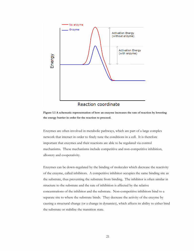
21

Figure 1.1 A schematic representation of how an enzyme increases the rate of reaction by lowering

the energy barrier in order for the reaction to proceed.

Enzymes are often involved in metabolic pathways, which are part of a large complex

network that interact in order to finely tune the conditions in a cell. It is therefore

important that enzymes and their reactions are able to be regulated via control

mechanisms. These mechanisms include competitive and non-competitive inhibition,

allostery and cooperativity.

Enzymes can be down-regulated by the binding of molecules which decrease the reactivity

of the enzyme, called inhibitors. A competitive inhibitor occupies the same binding site as

the substrate, thus preventing the substrate from binding. The inhibitor is often similar in

structure to the substrate and the rate of inhibition is affected by the relative

concentrations of the inhibitor and the substrate. Non-competitive inhibitors bind to a

separate site to where the substrate binds. They decrease the activity of the enzyme by

causing a structural change (or a change in dynamics), which affects its ability to either bind

the substrate or stabilise the transition state.

22

The binding of an effector at a site distal to the binding site that affects the rate of the

enzyme reaction is also termed allosteric regulation. In contrast to non-competitive

inhibition, allosteric effectors can also up-regulate an enzyme by changing the structure or

dynamics to favour the formation of the transition state. Usually the allosteric modulator

is heterotrophic (i.e. different from the enzyme’s substrate) but enzymes can be regulated

by their own substrate (homotrophic allostery). A special case of this is cooperativity.

Cooperativity occurs in a multimeric enzyme where the binding of the enzyme substrate

into the binding site on one subunit increases the affinity for the substrate in binding sites

on other subunits. Negative cooperativity can also occur where substrate binding on one

subunit reduces affinity for the substrate in other subunits. Two models have been

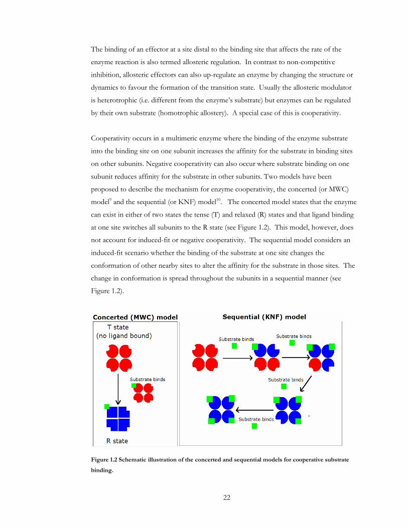
proposed to describe the mechanism for enzyme cooperativity, the concerted (or MWC)

model9 and the sequential (or KNF) model10. The concerted model states that the enzyme

can exist in either of two states the tense (T) and relaxed (R) states and that ligand binding

at one site switches all subunits to the R state (see Figure 1.2). This model, however, does

not account for induced-fit or negative cooperativity. The sequential model considers an

induced-fit scenario whether the binding of the substrate at one site changes the

conformation of other nearby sites to alter the affinity for the substrate in those sites. The

change in conformation is spread throughout the subunits in a sequential manner (see

Figure 1.2).

Figure 1.2 Schematic illustration of the concerted and sequential models for cooperative substrate

binding.

23

1.1.1.1 Enzyme Kinetics

The kinetics of non-cooperative enzymes with a single substrate can usually be described

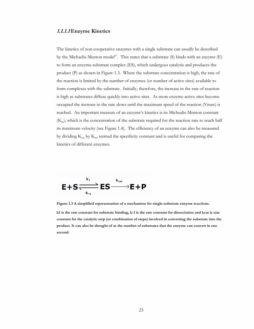
by the Michaelis-Menton model11. This states that a substrate (S) binds with an enzyme (E)

to form an enzyme-substrate complex (ES), which undergoes catalysis and produces the

product (P) as shown in Figure 1.3. Where the substrate concentration is high, the rate of

the reaction is limited by the number of enzymes (or number of active sites) available to

form complexes with the substrate. Initially, therefore, the increase in the rate of reaction

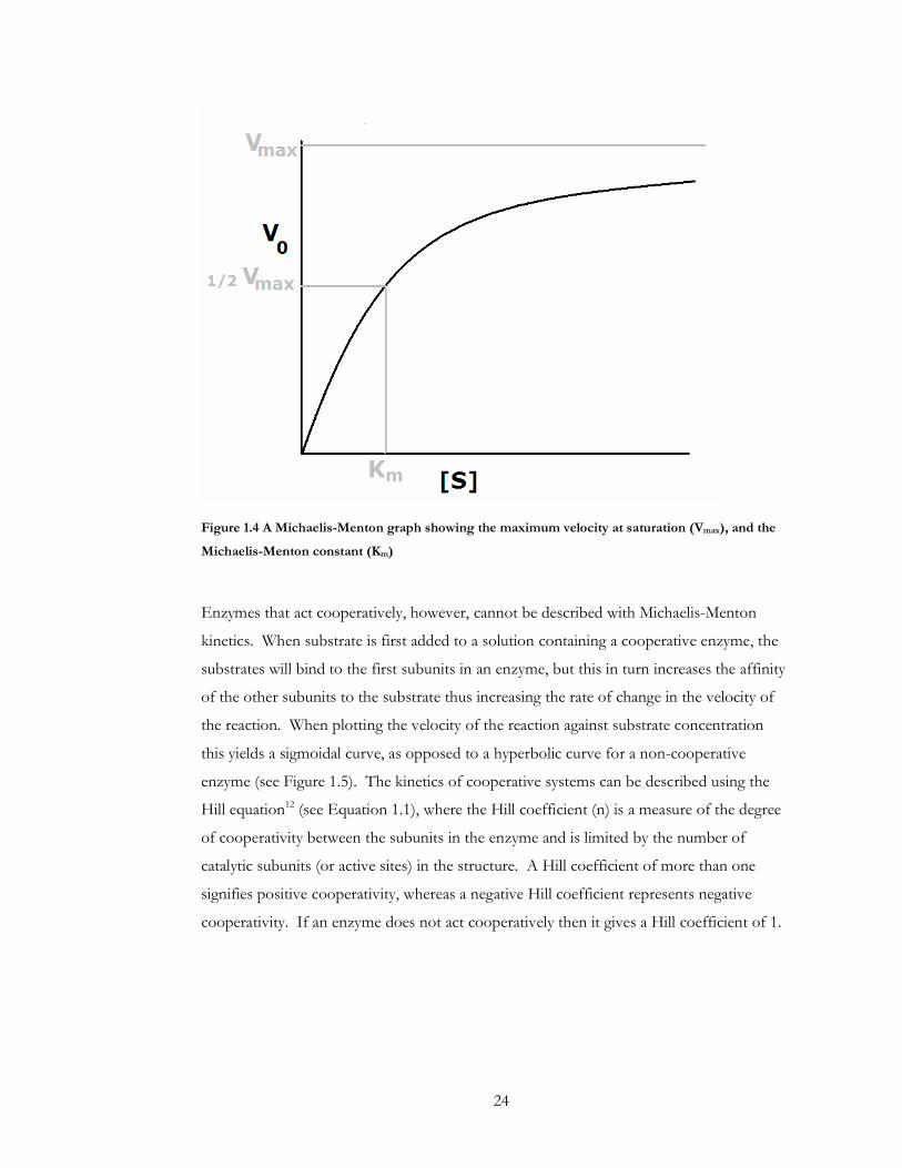
is high as substrates diffuse quickly into active sites. As more enzyme active sites become

occupied the increase in the rate slows until the maximum speed of the reaction (Vmax) is

reached. An important measure of an enzyme’s kinetics is its Michealis-Menton constant

(Km), which is the concentration of the substrate required for the reaction rate to reach half

its maximum velocity (see Figure 1.4). The efficiency of an enzyme can also be measured

by dividing Kcat by Km, termed the specificity constant and is useful for comparing the

kinetics of different enzymes.

Figure 1.3 A simplified representation of a mechanism for single-substrate enzyme reactions.

k1 is the rate constant for substrate binding, k-1 is the rate constant for dissociation and kcat is rate

constant for the catalytic step (or combination of steps) involved in converting the substrate into the

product. It can also be thought of as the number of substrates that the enzyme can convert in one

second.

24

Figure 1.4 A Michaelis-Menton graph showing the maximum velocity at saturation (Vmax), and the

Michaelis-Menton constant (Km)

Enzymes that act cooperatively, however, cannot be described with Michaelis-Menton

kinetics. When substrate is first added to a solution containing a cooperative enzyme, the

substrates will bind to the first subunits in an enzyme, but this in turn increases the affinity

of the other subunits to the substrate thus increasing the rate of change in the velocity of

the reaction. When plotting the velocity of the reaction against substrate concentration

this yields a sigmoidal curve, as opposed to a hyperbolic curve for a non-cooperative

enzyme (see Figure 1.5). The kinetics of cooperative systems can be described using the

Hill equation12 (see Equation 1.1), where the Hill coefficient (n) is a measure of the degree

of cooperativity between the subunits in the enzyme and is limited by the number of

catalytic subunits (or active sites) in the structure. A Hill coefficient of more than one

signifies positive cooperativity, whereas a negative Hill coefficient represents negative

cooperativity. If an enzyme does not act cooperatively then it gives a Hill coefficient of 1.

25

Figure 1.5 A plot showing the difference in change in reaction rate with the concentration between

cooperative and non-cooperative enzymes.

Equation 1.1 The Hill equation.

The Hill coefficient is denoted by n, Kd is the equilibrium dissociation constant, [L] is the

concentration of the ligand and θ is the fraction of binding sites that are occupied by substrate.

1.1.1.2 Enzyme Functions

The importance of enzymes in biological and evolutionary terms is evident in that all living

organisms contain enzymes. They are also practically important and its estimated that half

of all drug targets are classed as enzymes13,14. Whilst enzymes participate in the reaction

they are not considered as reactants as the enzyme remains chemically the same at the end

of the reaction. They contain highly specific active sites that dictate not only chemical

specificity but stereo- and regiospecificity. Catalytic residues use a wide variety of

mechanisms to catalyse each enzyme’s reaction, amongst which the most common are

stabilisation of intermediates, usually via electrostatic interactions and proton-shuttling

events15. Whilst enzymes involved in similar cellular functions can catalyse their reactions

via different intermediate steps, they can demonstrate propensity for certain reaction

26

mechanisms. Oxidoreductases, for example, tend to carry out their reactions by shuffling

electrons around their active site, whilst the transferase mechanisms tend to involve

nucleophillic addition and substitution15.

Molecular functions of enzymes are usually characterised by an E.C number, given

according to the Enzyme Commision (EC) classification scheme by the International

Union of Biochemistry and Molecular Biology (IUBMB)16. This is a hierarchical scheme

that represents individual enzymes by a four-digit number according the reaction it

catalyses. The EC number is given in the format a.b.c.d, where a represents one of the six

main classes, b denotes the sub-class, c represents the sub-subclass and d is the serial

number of the enzyme within the class (and usually translates to the substrate specificity).

27

The six main classifications of enzymes are;

1. Oxidoreductases (EC1)

This class of enzymes is involved in oxidation-reduction reactions where one

species is oxidised in order to reduce another. Oxidoreductases facilitate the

transfer of electrons from the reductant to the oxidant as is shown in Figure 1.6.

There are a further 22 subclasses of oxidoreductase that are differentiated by the

chemical group that they react on.

A- + B �� A + B-

Figure 1.6 A simple example of a redox reaction.

2. Transferases (EC2)

These enzymes are involved in reactions where a chemical group (rather than

electrons in the case of oxidoreductases) are transferred from a donor species to an

acceptor species (see Figure 1.7). Enzymes called kinases transfer a phosphate

group (usually fron ATP) to other donor molecules. Protein kinases transfer a

phosphate group specifically onto proteins and have important roles in regulation

and signaling.

A-X + B �� A + B-X

Figure 1.7 A simple example of a transferase reaction.

3. Hydrolases (EC3)

This is class with the largest amount of structural and sequence information (both

in terms of redundant and non-redundant sequences and structures, see Figure 1.9).

Their small size makes them easy targets for determination of their sequence and

structure, and therefore hydrolases were amongst the most popular early candidates

for structural determination. These enzymes catalyse hydrolysis reactions, where a

substrate is divided apart by the addition of water. One part of the substrate

accepts the proton and the other accepts the hydroxyl group as shown in Figure

1.8. There are 13 subclasses of hydrolases, which act on different chemical bonds.

A-B + H2O �� A-H + B-OH

Figure 1.8 A schematic equation for the hydrolysis reaction.

28

4. Lyases (EC4)

Like hydrolases, lyases break a chemical bond on their substrate to form two

molecules. Lyases, however, do not cleave the chemical bond by oxidation or

hydrolysis and act on bonds such as C-C, C-N and C-O. Lyase reactions usually

result in the elimination of a species from the substrate and the formation of a

double bond or ring structure in the remaining molecule. There are 7 subclasses of

lyases, depending on what kind of bond is cleaved.

5. Isomerases (EC5)

Isomerases catalyse the reaction that changes a substrate to a chemically identical,

but structurally different isomer. This can take form as a structural isomer, where

the chemical formula is the same but the bonds rearranged to form a different

structure, or a stereo-isomer where the structure is the same but the arrangement

of the groups in 3D space is different. There are 6 subclasses of isomerases, which

depend on the method of isomerisation. Three of these subclasses reflect reactions

that are catalysed by oxidoreductases, transferases and lyases, but are carried out

within the substrate (instead of on a second molecule) to create a single structurally

different product.

6. Ligases (EC6)

This is by far the smallest class of enzymes, perhaps as they have an energetically

difficult task. Ligases create a chemical bond which joins two chemical substrates,

often by hydrolysing a group from one or both of the substrate molecules. For

example, DNA ligase forms a phosphodiester bond between the 3' nucleotide and

the 5' phosphate group in a discontinuous strand of DNA and is involved in DNA

replication and repair.

29

Hydrolases (EC3) are the most abundant class of enzyme in sequence and structural

databases (even when accounting for the overrepresentation from redundant

sequences/structures, see Figure 1.9). There are small numbers of isomerase (EC5) and

ligase (EC6) structures in the PDB, however when duplicate structures are removed the

relative proportion of isomerases increases whilst the proportion of ligases remains low

(see Figure 1.9).

Figure 1.9 The proportion of each top EC class in the PDB.

The number of structures annotated is represented in panel A, whereas panel B represents the

number of non-redundant structures (i.e. do not contain subunits from the same SCOP

superfamily). This is also representative of the spread of enzyme functions seen in sequence

databases.

The relationship between EC classification and levels of sequence and structural similarity

is complicated. It has been shown that beyond the traditional function annotation

threshold of 40% sequence identity, EC number is widely conserved between proteins17,18.

Another study by Rost19, however, showed that EC classification is only fully conserved in

30% of enzyme pairs that exhibit more than 50% sequence identity. It is also unclear as to

how well EC classification is conserved in structurally similar proteins. In a study of 167

homologous structural CATH superfamilies17 it was shown that almost half contained

enzymes that had differing EC classifications. Whilst most of these differences were in the

fourth digit, 22 of the superfamilies had EC numbers that differed at all levels. Similarly,

there is evidence of structural differences within EC classifications. Approximately 8.5%

(185) of the total number of EC nodes (full four-digit numbers) in the classification

scheme contain two or more enzymes that are structurally unrelated20. There is therefore

evidence that enzyme function has evolved via both divergent and convergent evolution.

30

1.2 Computationally determining protein function

Knowledge of protein function is fundamental to elucidating the exact mechanisms of

biological process within the cell. Understanding these processes is important in

developing therapeutic agents and identifying drug targets. Biochemical studies of a

protein’s function can be lengthy, expensive and sometimes fruitless and therefore

computational methods have been developed to try to predict a proteins function without

experimentation. The most common approach for this is by inferring function from a

similar protein of known function. Similar proteins are identified based either on the

degree of similarity between their sequences or three-dimensional structures.

As it has been observed that evolution is more tightly constrained for the structure of a

protein than it is for its sequence 21, structural information is increasingly being used to

identify a protein’s function. Due to the wealth of functional information held in these

structures and the recognition that the protein structures available only represented a

proportion of the total fold space thought to exist, there has been a change in the way

protein structures are solved.

Traditionally a protein’s structure was solved once the protein’s function had been

characterised with a view to understanding the exact mechanisms of its function. The

structural genomics initiatives have reversed that practice22 and many structures are now

being produced for proteins that have little functional characterisation in order to provide

insight into its biochemical function.

This has created a huge surge in the number of protein structures being deposited into the

Protein Data Bank1 (PDB). Over the past 5 years the number of structures in the PDB has

risen from 16,466 to just over 66,000 (see Figure 1.10). There is however a limited capacity

of laboratories to experimentally study each of these proteins and as a result there has been

an increase in the number of protein structures in the PDB with an ‘unknown function’

annotation from 19 to over 1500 in the last 5 years.

1 http://www.rcsb.org/pdb/

31

Due to the drive to produce structures for proteins that inhabit fold space not represented

in the current set, some of the structures produced may not exhibit similarity to another

functionally annotated protein. This is one of the reasons for the increase in the number

of proteins that cannot be assigned a function by similarity. There is therefore a need for

new methods to predict function without transfer of annotation via similarity.

0

10000

20000

30000

40000

50000

60000

70000

1986 1988 1990 1992 1994 1996 1998 2000 2002 2004 2006 2008 2010

Year

Nu

mb

er

of

str

uctu

res in t

he

PD

B

Figure 1.10 The rise in the number of structures deposited into the PDB since 1986.

32

1.2.1 Defining Protein Function

Defining what is meant by protein function is fundamental to the task of protein function

prediction. There is much ambiguity in the definition of protein function due to the fact

that it depends upon the context in which it is used. This has resulted in a range of

biological classification schemes which could differentially annotate a given protein.

The main source of confusion over the definition of protein function is due to the multi-

dimensional nature of the way function can be thought of. For example, trypsin can be

classified according to its biochemical function (peptide bond hydrolysis), molecular

function (a proteolytic enzyme), cellular role (protein degradation) or physiological role

(e.g. digestion). It could be even further complicated by considering cellular location or

regulatory roles.

Another issue when classifying protein function is that often proteins exhibit multiple

functions. The average number of experimentally verified functions for proteins in the

Gene Ontology Annotation project (GOA) is 1.35 23, showing that proteins have a

tendency to carry out more than one function. Multi-functionality may be inherent in its

role (for example, the lac repressor has a role in both carbohydrate metabolism and

osmoprotection) or circumstantial (RNA polymerase enzyme function can considered to

be different at the various stages of the transcription cycle, because the reactions it

catalyses are very different).

1.2.1.1 Classification Schemes

One of the first attempts to classify proteins with regards to their function was the Enzyme

Commission (EC) classification scheme24, which was first developed in 1955. As detailed

above, the EC classification scheme consists of six principle classes of enzymes, which are

then further broken down into 3 further levels with respect to reaction mechanisms,

reactants and products and lastly specificities. Each of these categories (and subsequent

sub-categories) is associated with numerical values, thus each classification of an enzyme

can be represented by a number in the format a.b.c.d.

33

The main advantage of the EC classification is its controlled vocabulary which lends itself

to computational analysis because of its numerical representation. Whilst the EC

classification is simple and well established, it does have properties that make it

problematic for use in bioinformatics analyses. Firstly, the classes are inconsistently

defined by using substrates, transferred groups and acceptor residues in different ways.

Secondly, enzymes are classified based on the overall reaction that they catalyse. The

reaction may consist of multiple sub-reactions catalysed by the enzyme but the

classification number will only represent the overall reaction mechanism. Another point

worth noting is that EC numbers are associated with the reaction catalysed not the protein.

Therefore enzymes that have similar EC numbers are not always evolutionarily similar or

take part in a similar cellular role.

Whilst useful, the EC numbering system only applies to enzymes and therefore other

classification methods have been developed to cover a wider range of protein functions.

The first more comprehensive classification scheme to cover products of a whole genome

was developed by Riley, who proposed a classification scheme based on the physiological

function for products of the E.Coli genome25. An updated version of this scheme was

implemented in GenProtEC 26,27. This classification scheme became the basis for others

such as TIGR28 and SubtiList29.

In the early days a series of classification schemes developed for a species specific database

such as Saccharomyces Genome Database (SGD)30 and Yeast Protein Database (YPD)31, that

contain species specific derivatives. Whilst these classification schemes only apply to

specific species, some of these schemes have been expanded to include other organisms.

For example, MIPS/PENDANT started out as a yeast specific classification but has been

modified to include many other species32.

Instead of focusing on a specific species or type of protein, some classification schemes

focus around specific types of functions. The Kyoto Ontology, which is implemented in

the KEGG PATHWAY database5 and the What Is There (WIT, now renamed as

ERGO)33 mainly address regulation and metabolic pathways. Other schemes may classify

based on another aspect of function such as location, for example YPL.db34, or molecular

interactions35-37.

34

Most of these classification schemes can be thought of as trees, whereby progression along

the tree from top to bottom represents increasingly specific functions. There is, however,

a move away from the traditional tree structure towards a more complex organisation. The

Gene Ontology (GO) classification scheme38 is one of the first classification schemes to

move away from this simple tree structure. The GO scheme seeks to remove some of the

ambiguity that exists in other databases by classifying function based on three different

areas; molecular function, biological process and localisation to cellular components. This

increase in complexity over tree-based schemes presents ease of use and navigation issues,

and lends itself less to computational analyses.

When approaching the task of predicting protein function, it is important to consider what

is meant by function and therefore which classification scheme to use. The coverage of

proteins in functional classification schemes can vary depending on the individual protein

(see Table 1.1). Due to lack of coverage and consistency in how function is described

using different classification schemes, the development of a single unified scheme would

be desirable. Whilst there are some efforts being made into the development of a unified

classification scheme39, there is a lack of a clear consensus on how to tackle this problem.

35

Protein ID Coverage of functional annotation schemes (%)

Annotation

CT080 15 Late transcription unit B hypothetical Protein

CT094 25 tRNA pseudouridine synthase CT313 30 Transaldolase EC 2.2.1.2 CT664 25 FHA domain-containing protein

Table 1.1 A table showing how the coverage of classification schemes varies per protein.

Adapted from Ouzounis et al.40. Examples of four randomly selected proteins from the Chlamydia

trachomatis serovar D genome sequence41 and their annotations. The coverage of consistent

annotations for the 20 functional classification schemes is shown as a percentage. The 20

classification schemes analysed are listed in the original publication40.

1.2.2 Functional Transfer Based on Homology

Functional annotation of proteins by biological experimentation is generally slow and

expensive in terms of time and resources and therefore computational techniques are often

used. The most widely used technique takes advantage of structural or sequence

similarities between proteins that have evolved from a common ancestor and therefore

may exhibit similar functionality.

Although the transfer of functional annotation by homology is very powerful, it has

limitations and has been blamed as one of the main sources of error for incorrect

functional annotation in current databases42,43. One such limitation is that there may be a

lack of an accurately annotated homologue in the databases from which to transfer

functional information. It has been estimated that ~25% of newly sequenced genes have

no annotated homologue44 and the ability to detect homologues decreases as the sequence

similarity threshold (and therefore the accuracy of annotation transfer) is raised (see Figure

1.11).

A second problem faced by this method is the level of similarity required to enable

accurate transfer of functional information is unclear. Indeed, there are even differences in

the level of sequence identity required to transfer different types of functional annotation

36

(see Figure 1.11). Several groups studied the relationship between sequence identity and

functional conservation and, despite using different approaches, agree that below 50%

identity functions diverge very quickly17,18,45,46. Rost, however, argued that these types of

simple pairwise comparison studies might be misleading due to database bias and suggested

that annotation transfer cannot be reliably employed below 70% sequence identity19. Tian

and Skolnick later carried out an analysis similar to Rost, which also took into account

database bias47. This suggested that a 40% threshold can still be used as a confident

threshold for functional transfer.

Ultimately, however, protein function can differ on a small number of changes in amino

acid composition and therefore even when transferring annotation for highly similar

proteins, errors can still occur. For example, the acidic endochitinase WIN6.2b precursor

sequence exhibits 94% sequence identity with DNA topoisomerase II (β-isozyme) despite

them having different functions (EC numbers 3.2.1.14 and 5.99.1.3 respectively)19.

One of the biggest dangers of this method is the prospect that it may propagate any

existing errors in the database, thus amplifying the effects of one incorrect annotation

across a potentially large number of annotations. A study by Jones et al. suggests that

almost half of all annotations assigned by sequence similarity in the GOSeqLite database

are erroneous48. Once an incorrect annotation has been transferred there is the

opportunity for the amount of annotation errors to spread rapidly throughout the database.

37

Figure 1.11 The accuracy of function annotation with varying sequence identity (adapted from Rost

et al.19)

(A) Accuracy of annotation transfer according to percentage sequence identity. The black line

indicates subcellular location annotation and the purple line indicates enzymatic function

annotation. (B) The power of transfer of annotation according to the sequence identity threshold

used for annotation transfer. The arrows represent points in the curve where the error margin is 10%

(i.e. 10% of the annotations are incorrect).

38

1.2.2.1 Sequence Similarity

Assessing sequence similarity to evaluate whether two proteins are homologs and therefore

are likely to share common functionality is the most widely used method of predicting

function. Even with the rapidly growing number of protein structures, the amount of

structural data is far out-weighed by the availability of sequence data and therefore

sequence data is still favoured for use in comparative studies.

Various tools exist to assess the level of similarity between sequences such as BLAST49,

PSI-BLAST50 and FASTA51, which compare a given sequence to sequences deposited in

the major sequence databases (see Table 1.2).

Database URL Reference

DDBJ (DNA Data

Bank of Japan)

http://www.ddbj.nig.ac.jp/ 52

GenBank http://www.ncbi.nlm.nih.gov/Genbank/index.ht

ml

53

EMBL Nucleotide

DB

http://www.ebi.ac.uk/embl/index.html 54

Table 1.2 The main primary sequence databases with their URL and relevant reference.

Kellar et al. highlighted the hazards of basing annotations on sequence similarity alone,

without considering the protein structure55. They suggested that CbiT, which is involved in

vitamin B12 biosynthesis, is a methyltransferase based on structural similarities between the

crystal structure of CbiT and other methyltransferases. This was then later confirmed by

experimentation. However, CbiT was previously annotated as a decarboxylase based upon

sequences similarities with other decarboxylases.

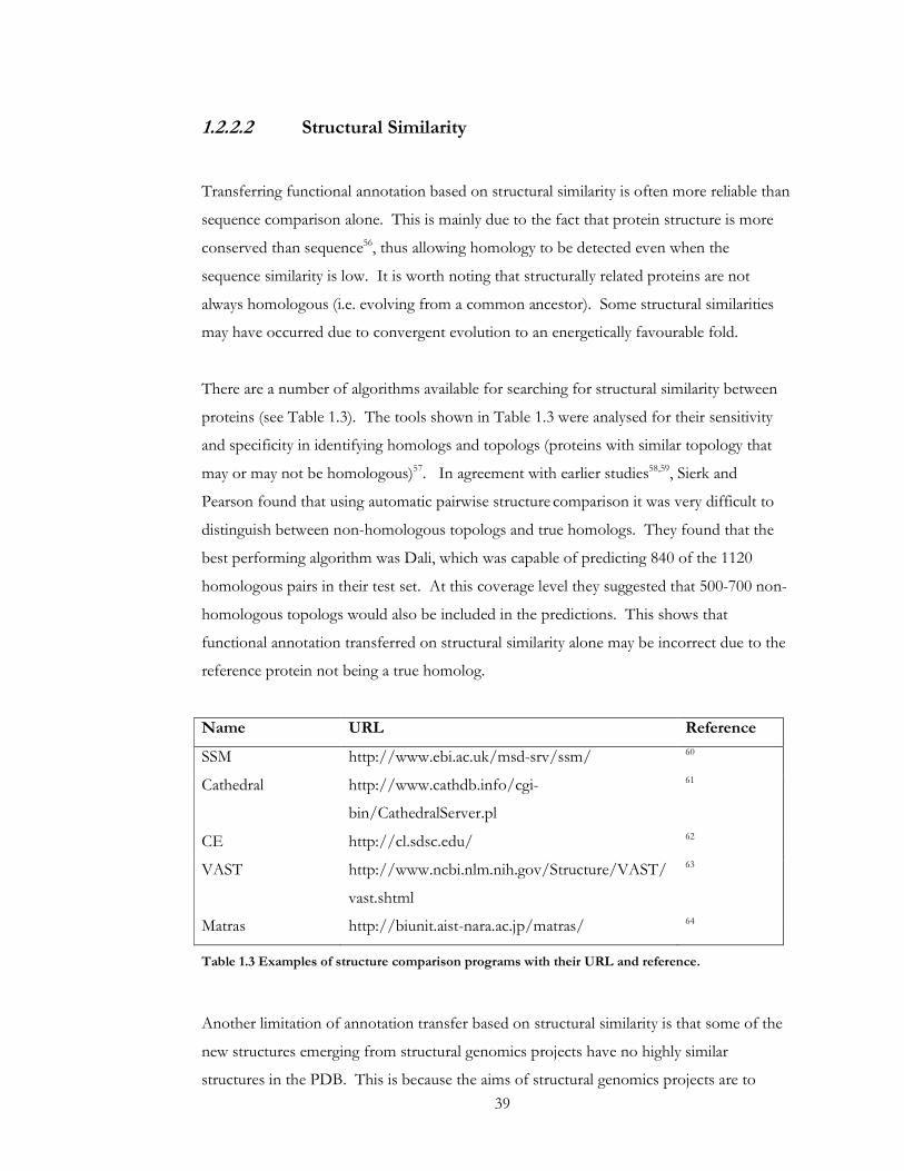
39

1.2.2.2 Structural Similarity

Transferring functional annotation based on structural similarity is often more reliable than

sequence comparison alone. This is mainly due to the fact that protein structure is more

conserved than sequence56, thus allowing homology to be detected even when the

sequence similarity is low. It is worth noting that structurally related proteins are not

always homologous (i.e. evolving from a common ancestor). Some structural similarities

may have occurred due to convergent evolution to an energetically favourable fold.

There are a number of algorithms available for searching for structural similarity between

proteins (see Table 1.3). The tools shown in Table 1.3 were analysed for their sensitivity

and specificity in identifying homologs and topologs (proteins with similar topology that

may or may not be homologous)57. In agreement with earlier studies58,59, Sierk and

Pearson found that using automatic pairwise structure comparison it was very difficult to

distinguish between non-homologous topologs and true homologs. They found that the

best performing algorithm was Dali, which was capable of predicting 840 of the 1120

homologous pairs in their test set. At this coverage level they suggested that 500-700 non-

homologous topologs would also be included in the predictions. This shows that

functional annotation transferred on structural similarity alone may be incorrect due to the

reference protein not being a true homolog.

Name URL Reference

SSM http://www.ebi.ac.uk/msd-srv/ssm/ 60

Cathedral http://www.cathdb.info/cgi-

bin/CathedralServer.pl

61

CE http://cl.sdsc.edu/ 62

VAST http://www.ncbi.nlm.nih.gov/Structure/VAST/

vast.shtml

63

Matras http://biunit.aist-nara.ac.jp/matras/ 64

Table 1.3 Examples of structure comparison programs with their URL and reference.

Another limitation of annotation transfer based on structural similarity is that some of the

new structures emerging from structural genomics projects have no highly similar

structures in the PDB. This is because the aims of structural genomics projects are to

40

obtain structures for regions of protein fold space that are currently under-represented in

the PDB.

1.2.2.3 Dynamic Similarity

The mechanisms of most protein functions require some sort of dynamic motion to elicit

their effect, either by small fluctuations in residue side chains or large-scale conformational

changes. The increase in computational power has allowed the estimation of protein

motion by approaches such as molecular dynamics and also by more simplified approaches

based on normal mode analysis. Since it is widely accepted that proteins with similar

sequence or structure are likely to have similar function, it may also carry that similarity in

dynamics can be used to transfer annotation.

Early attempts at aligning the dynamics of proteins relied on first creating a structural or

sequence alignment to create reference points from which to compare dynamics65,66.

Further studies have proposed other methods that either loosely constrain the alignment

by structure67 or attempt to align the dynamics without prior structural alignment at all68.

The study of the dynamic similarity between families of proteins has shown that similarities

in dynamic behaviour can be detected66 and can allow clustering within these families that

is reflective, not only of clusters of structural similarity, but of clusters of similar

mechanisms or functions68,69. In a study of representative protease structures from

different folds, the dynamic properties were shown to be strongly conserved, particularly

around their functional site, despite their lack of similarity in structure and sequence70.

This suggests that convergent evolution may also act to produce dynamics that are essential

for a particular function in the same way as is thought of for structure.

The results of these studies suggest that functional annotation may be able to be

transferred by detection of similar dynamic properties. However, a study of the dynamic

similarity between representative enzymes from the main functional and structural classes

showed that dynamics are inconsistently conserved between members of the same

functional class67,70. It was, however, possible to detect a subset of homologous protein

pairs by dynamic alignment alone that would not have been detected using usual structural

or sequence comparison thresholds.

41

1.2.3 Predicting Protein Function in the Absence of Sequence or

Structural Similarity

It is estimated that 25% of known sequences show no homology to any annotated

sequence with a further 37% exhibiting levels of sequence similarity that may give rise to

unreliable annotation by automatic transfer44. This provides a large set of proteins for

which homology based methods fail. There has been much recent effort in developing

new methods to predict protein function without the traditional global alignment followed

by functional transfer. These methods use a wide variety of properties and methods using

both sequence and structural attributes. As no single approach is 100% accurate, it is

becoming increasingly important to combine approaches. This integrated approach to

function prediction is implemented in several servers such as ProKnow 71 and ProFunc 72.

1.2.3.1 Sequence Motifs

Even in the absence of overall sequence similarity, a common motif (an isolated sequence

pattern) or fingerprint (a number of sequence patterns) are often observed in proteins that

carry out the same function. Whilst the construction of sequence motifs often involves the

detection of homologs (see Figure 1.12), sequence motifs can be used without having to

infer homology by whole sequence similarity.

There are several motif databases, each with their own search tools (see Table 1.4).

Sequence motifs from PROSITE73 and PRINTS74 are presented in the integrated protein

annotation database INTERPRO75 in an attempt to combine the strengths of motifs with

other annotation methods. Machine learning techniques have also been applied to

functional annotation using sequence motifs. One example is the Anagram server76, which

uses the protomotifs (subtle amino acid patterns) as features of different functional classes

in SWISS-PROT to train a support vector machine algorithm to predict functional

classification.

42

Figure 1.12 Schematic diagram of a generic approach for constructing sequence motifs

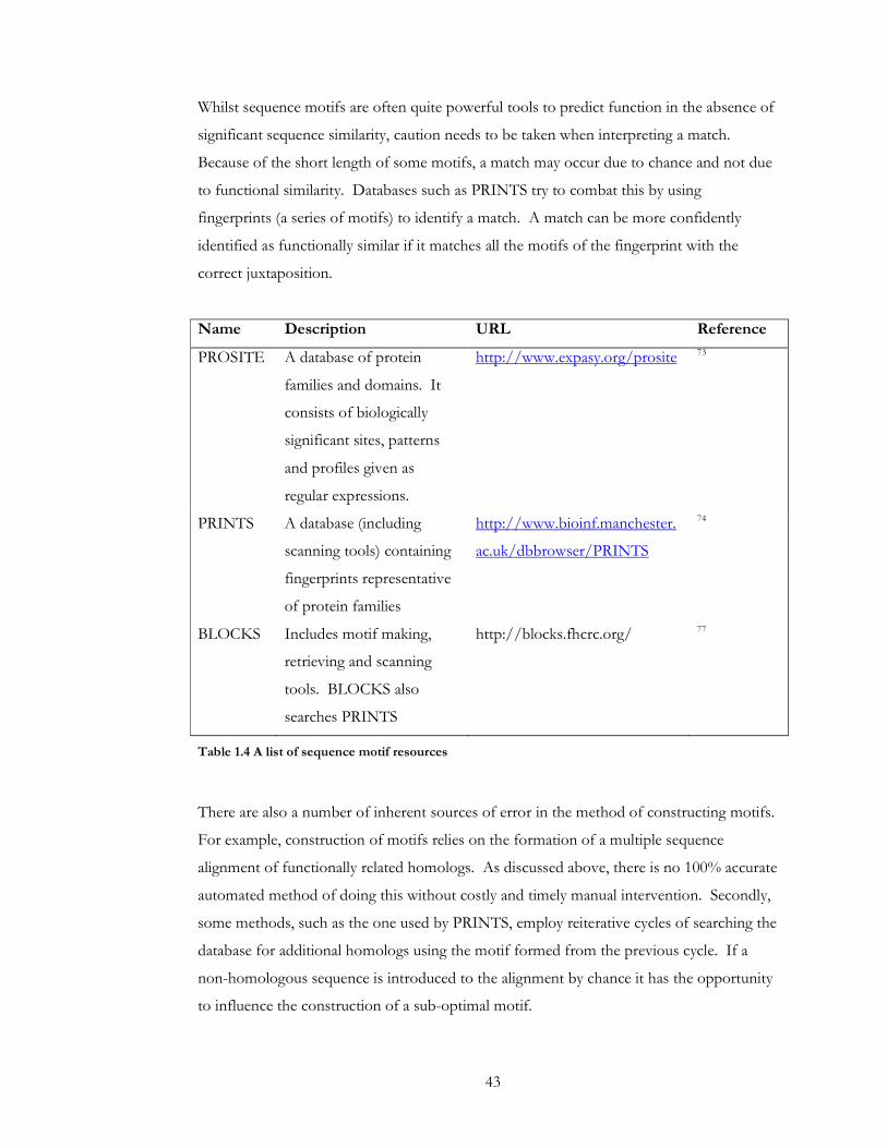
43

Whilst sequence motifs are often quite powerful tools to predict function in the absence of

significant sequence similarity, caution needs to be taken when interpreting a match.

Because of the short length of some motifs, a match may occur due to chance and not due

to functional similarity. Databases such as PRINTS try to combat this by using

fingerprints (a series of motifs) to identify a match. A match can be more confidently

identified as functionally similar if it matches all the motifs of the fingerprint with the

correct juxtaposition.

Name Description URL Reference

PROSITE A database of protein

families and domains. It

consists of biologically

significant sites, patterns

and profiles given as

regular expressions.

http://www.expasy.org/prosite

73

PRINTS A database (including

scanning tools) containing

fingerprints representative

of protein families

http://www.bioinf.manchester.

ac.uk/dbbrowser/PRINTS

74

BLOCKS Includes motif making,

retrieving and scanning

tools. BLOCKS also

searches PRINTS

http://blocks.fhcrc.org/ 77

Table 1.4 A list of sequence motif resources

There are also a number of inherent sources of error in the method of constructing motifs.

For example, construction of motifs relies on the formation of a multiple sequence

alignment of functionally related homologs. As discussed above, there is no 100% accurate

automated method of doing this without costly and timely manual intervention. Secondly,

some methods, such as the one used by PRINTS, employ reiterative cycles of searching the

database for additional homologs using the motif formed from the previous cycle. If a

non-homologous sequence is introduced to the alignment by chance it has the opportunity

to influence the construction of a sub-optimal motif.

44

1.2.3.2 Functional Sites

Analysing the features of functional sites and using them to predict function seems logical

since it is the part of the protein which is arguably most important to protein function.

Whilst the rest of the protein may have roles such as stabilising or trafficking the protein,

the functional site contains the most information about the specific function of the protein

and therefore may be the most useful part to study in order to assign function.

It is important to point out that there is ambiguity in what is meant by a ‘functional site’.

In some cases a binding site may be considered to be a protein’s functional site, especially

in cases where enzymes bind their substrate in their catalytic site. However, proteins such

as G- protein coupled receptors bind a ligand on their extracellular C-terminal end and

elicit their response on their intracellular C-terminal domain. In this case, the site that

actually elicits its function is separate from its ligand binding site. Indeed, both the ligand

binding site and the G-protein coupled site could be considered to be functional sites.

Enzymes lend themselves to binding site analysis since they have well defined active sites.

It is also worth noting that some proteins, such as structural proteins, have no obvious

functional site.

45

Name Description URL Reference

PdbFun A database compiling annotated residues from the PDB. Contains binding site residues using the HETERO groups from the PDB and catalytic residues from CATRES

http://pdbfun.uniroma2.it/

78

PDBSiteScan/PDBSite

PDBSite is a database containing functional sites extracted from PDB using the SITE records and of an additional set containing the protein interaction sites inferred from the contact residues in heterocomplexes. PDBSiteScan provides structural alignment with known functional sites stored in PDBSite.

http://wwwmgs.bionet.nsc.ru/mgs/gnw/pdbsitescan/

79

PINTS A server that can compare a protein structure against a database of patterns or a structural pattern against a database of protein structures

http://www.russell.embl.de/pints/

80

PROCAT/TESS/Jess/Catalytic Site Atlas

The Catalytic Site Atlas (CSA) is a database documenting enzyme active sites and catalytic residues in enzymes of 3D structure.

http://www.ebi.ac.uk/thornton-srv/databases/CSA/

81

pvSOAR Detects surface similarities in protein structures. It allows a user to search a protein surface pattern derived from a pocket or a void against all known surface patterns from the CASTp (Computed Atlas of Surface Topology of proteins) database

http://pvsoar.bioengr.uic.edu/

82

SPASM/RIGOR A server that takes PDB style residue coordinates of a motif or template and searches them against known motifs based in a database derived from the PDB

http://portray.bmc.uu.se/cgi-bin/spasm/scripts/spasm.pl

83

SuMo Screens the PDB for protein structures that match a binding site in a given protein structure. It uses its own heuristics for defining ligand binding sites

http://sumo-pbil.ibcp.fr/

84

Table 1.5 Functional/active/binding site residue databases and comparison tools available via the

web.

46

In a similar way to homology-based annotation, information about active sites can be used

to transfer annotation. There are many resources that store structural and sequence

information about known active sites of proteins with well characterised function (see

Table 1.5). A protein of unknown function can be compared to these resources to identify

any similarities with known active sites. One such tool, the Structure-Function Linkage

Database85 organises enzymes into groups defined by highly conserved residues in the

active site that are thought to be related to the reaction that members of that group

mediate. An uncharacterized protein can then be assigned to a reaction group based on

whether it possesses these specific active site residues in the corresponding locations.

Unlike transfer of annotation via homology, such methods do not rely on finding a match

with significant overall sequence or structural similarity. A match can be detected even if

the less evolutionarily constrained parts of the protein have diverged, making them

undetectable to traditional homology searches. Indeed, this method can find proteins with

similar function that have evolved through convergent evolution to some favourable active

site formation.

Other methods of predicting protein function by using active site information do not rely

on finding similarity between existing active sites on other characterised proteins. Instead,

they identify functional sites using the geometry (SARIG86), chemistry (WEBFEATURE87,

THEMATICS88) or electrostatic properties89,90 of a site. These properties may be

associated with a function and therefore can be used to predict the functional class of

given protein. An approach to finding a functional site using electrostatic properties90

illustrated that they were also able to use these properties to discriminate between enzymes

and non-enzymes.

There are other methods for finding functional sites that require alignment with known

homologs such as Evolutionary Trace (ET). ET identifies and orders amino acids

variations in a diverging phylogenetic tree 91. The least varied (most conserved) amino

acids have been shown to correlate well with functional sites and thus ET has been used in

several methods of functional site detection 92-95. One of the problems with this method,

however, is that residues may be conserved for reasons other than to maintain the active

site, such as for the preservation of a favourable structure. Cheng et al. have developed a

method that predicts sequence profiles expected purely under structural constraints and

47

then uses them to predict whether an observed conservation pattern is due to structural or

evolutionary constraints 96. In a similar approach Cheliah et al., construct profiles of

conservation that are expected under functional and structural constrains and use this to

identify regions of the protein that are conserved for functional reasons95.

1.2.3.3 Genomic Context

The ability to predict the function of a protein by considering its genomic context is based

upon four theories. Firstly, functionally similar proteins often evolve in a similar manner.

The measure of a gene’s presence or absence from a set of genomes over an evolutionary

period is termed phylogenetic profiling 97. Function is predicted by matching the

phylogenetic profiles of the unknown protein to those which are known. Barker and Pagel

predicted functional associations by mapping absence/presence data of gene pairs over 15

species’ genomes 98.

Secondly, genes of functionally related proteins may exist in an order which is conserved in

a number of genomes (the Gene Neighbour method)99,100. Thirdly, functionally related

genes may exist as part of an operon101, and lastly, they may fuse to form a novel single

gene in another genome (the Rosetta Stone method 102, see Figure 1.13). The disadvantage

with the latter approach is that it relies on one of the fused domains to have a known

function. If both fused genes are uncharacterised then very little can be inferred.

48

Figure 1.13 A schematic representation of the Rosetta Stone method of assigning protein function.

Coloured blocks represent genes, with sections of the same colours representing sequence

similarity. Sequence A is from an uncharacterised protein, which is found to have high sequence

similarity to an isolated section (in red) of a gene in sequence B in another genome, although it may

not show significant overall sequence similarity to be considered to be homologous. The other non-

similar section (in blue) of sequence B has a high level of sequence similarity to another sequence,

C. The protein of sequence C is functionally characterised and therefore it can be inferred that

protein A is functionally similar to C since they appear to have fused to form protein B.

There are several tools that utilise these basic concepts to predict function. Phydbac103

uses phylogenetic profiles, chromosomal proximity and the Rosetta Stone method to

predict function using GO terms. Another tool, SNAP104, adds to these approaches by

constructing graphs of similarity versus neighbourhood (proximity) for co-located and

homologous genes of bacterial genomes. Functionally related genes are thought to exhibit

similar graphs.

Although there has been some success using these methods, they tend to work better in

prokaryotes, especially the operon and gene-ordering based methods. Gene order-based

functional prediction seems to be almost impossible for eukaryotes as they apparently lack

functional gene clusters.

49

1.2.3.4 Protein-Protein Interactions

It is often observed that proteins carry out their function as a group of proteins that

physically interact with each other. For this reason function can be inferred of an

uncharacterised protein if it is shown, or predicted, to interact with a protein of known

function. Attempts have been made to map GO terms to uncharacterised proteins using

protein-protein interactions with reasonable success 105-108.

There are many databases holding experimentally derived protein-protein interaction

information36,109,110, however it is unlikely that when trying to annotate a hypothetical

protein there will be any experimental interaction data available for that protein. Thus,

protein-protein interaction prediction methods are needed to be able to predict any

interaction and therefore a possible shared function with another protein.

There have been many different approaches to predicting protein-protein interactions.

Pazos et al. have developed a method, which uses correlated mutation analysis to predict

true protein-protein interactions and suggests likely regions for the interaction interface111.

The same group also proposed a method that uses similarity between the evolutionary

distance between the sequence of the proposed interacting pairs112. Another approach

looks at unusually exposed amino acids as an interaction site predictive feature113.

As with the Rosetta stone method, the major drawback of this method is the fact that to be

able to predict a function for a protein, the predicted interaction partner has to have a

known function.

50

1.2.3.5 Subcellular Localisation

It is possible to use subcellular location as a feature to use for predicting protein function

as it is reasonable to assume that proteins must be co-localised within the same subcellular

compartment in order to cooperate in a shared function. Also certain functions are

indicative of subcellular localization (i.e. DNA ligases are often found in the nucleus).

Proteins need to be transported from where they are made to the location where they carry

out their function. In order for the cell to successfully traffic these proteins they contain

sorting signals in their amino acid sequence 114,115. This prompted studies which revealed

that localisation correlates with total amino acid composition and sequence motifs (signal

sequences). This has led to the development of a number of methods based around the

analysis of amino acid composition116,117. Phylogenetic profiling has also been used to

predict localisation118, but it has been less successful than using amino acid composition.

Some tools have attempted to combine the amino acid composition approach with other

methods such as searching databases of known signal sequences119 or analysing expression

levels120. One other approach by Drawid and Gerstein121 was to use a diverse range of 30

features in a Bayesian probabilistic approach, which updates a protein’s probability that it is

found in a given subcellular component.

51

1.2.3.6 Structural Features

Since structure is more highly conserved than sequence, analysing structural features may

give clues to a protein’s function. Not only can structural information be used as a

comparative tool to transfer annotation by homology but also as a direct tool to predict

function.

In a similar way to sequence motifs, structural motifs or patterns are used to identify a

protein with a similar function. These can be residue based motifs 122 or motifs based on

geometric and chemical similarity 123. As a proteins function is strongly associated with a

‘functional site’, for many proteins such as enzymes or binding proteins the best structural

motif classifiers are their active site or binding site. However, there are some tools that

attempt to predict function by using 3D templates not solely limited to information from

functional sites124. Espadaler et al. have developed a method to look at the properties of

loop regions as predictors of function without defining the functional site125.

Rather than use short 3D motifs, some approaches use more global structural features to

define function. From a study of structural features of the proteases, Stawiski et al. found

that they exhibit similar characteristics such as smaller than average surface areas and

higher Cα densities, regardless of whether or not they were evolutionarily related126. They

also showed different secondary structure content to the non-proteases. By using these

features in a machine learning approach they were able to define a set of structural

classifiers that could predict whether a protein is a protease or non-protease with an

accuracy of over 86%. In a later study, Stawiski et al. also reported structural features that

are characteristic of the O-glycosidases such as distinctive electrostatic properties of the

proteins surface, despite differences in the overall fold127.

52

Whilst the above studies are limited to a subset of protein functions, attempts have been

made to use similar structural features to classify proteins into more generic subsets.

Dobson and Doig used 52 simple structural features (see Figure 1.14) in a support vector

machine-learning algorithm to distinguish between enzymes and non-enzymes 128. These

52 features were culled to a set of 36 (the bold items in Figure 1.14) best performing

features, which increased the predictive accuracy from 77% to 80%. A later study129

attempted to classify the enzyme predictions further into the top EC classification number

with an overall accuracy of 35% with the top ranked prediction, increasing to 60% with the

top two ranked predictions. These studies however, focused on global structural features

(for example, overall size or amino acid composition) and since the active site of an

enzyme is more closely associated with its function, it is hypothesised that these methods

could be improved upon by including structural features specifically of an enzymes active

site.

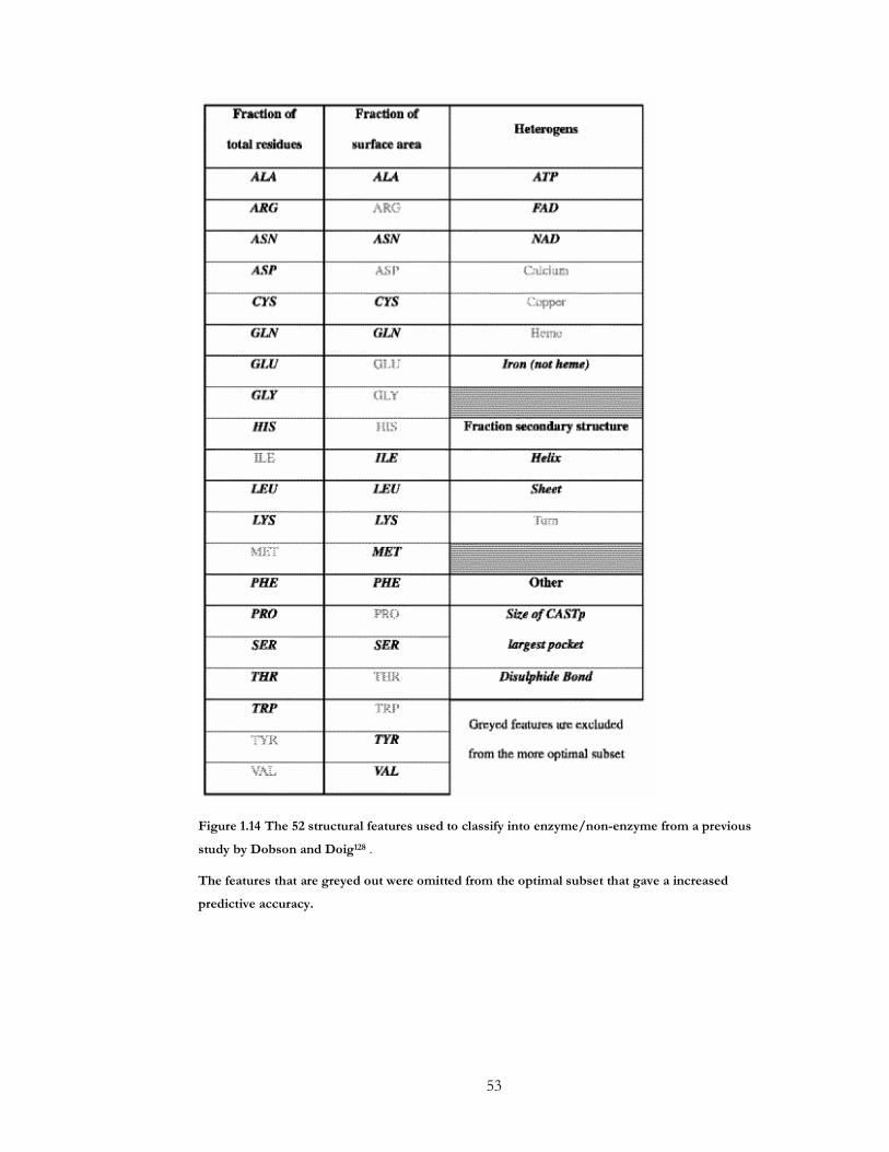
53

Figure 1.14 The 52 structural features used to classify into enzyme/non-enzyme from a previous

study by Dobson and Doig128 .

The features that are greyed out were omitted from the optimal subset that gave a increased

predictive accuracy.

54

1.3 Thesis Structure

The initial aim of this work was to continue the work by Dobson and Doig129 in looking at

the relationship between sequence and structural features of enzymes and their function.

Previous work focused on producing a computational method to predict the functional class

(top EC classification) of an enzyme based on these features. The machine learning method

used in this work, however, made the interpretation of the exact relationships between the

features and the enzyme function difficult. In Chapter 2 of this thesis, a study of the

differences in structural and sequence features of a non-redundant set of enzymes and their

active sites explores the structure-function relationship and further investigates those

features that differ the most between functions.

Furthermore, improvement to the performance of the previous functional prediction

method was attempted by the inclusion of active-site specific features (Chapter 4). In order

for this tool to be applicable to proteins with little or no characterisation, it was necessary to

predict the location of the functional site on the enzyme. Chapter 3 details a comprehensive

benchmark study of current publicly-available software for the prediction of functional sites

and also presents the creation of a webserver to deliver a previously published method by

this group90,130.

In order to further study one of the main findings in Chapter 2, a method to detect

cooperativity in enzymes by assessing the communication in dynamics between residues in

different subunits of oligomers was attempted in Chapter 5. This chapter also goes on to

further investigate the dynamic properties of oligomers in general.

The work contained in Chapter 2 (and some in Chapter 4) has been published as an article in

J. Mol. Biol131. The work in Chapter 3 has been published as an article in BMC

Bioinformatics132 and the work in Chapter 5 is written as a manuscript and currently in

review.

55

1.4 References

1. Apweiler R MM, O'Donovan C, Magrane M, Alam-Faruque Y, Antunes R, Barrell D, Bely B, Bingley M, Binns D, Bower L, Browne P, Chan WM, Dimmer E, Eberhardt R, Fedotov A, Foulger R, Garavelli J, Huntley R, Jacobsen J, Kleen M, Laiho K, Leinonen R, Legge D, Lin Q, Liu W, Luo J, Orchard S, Patient S, Poggioli D, Pruess M, Corbett M, di Martino G, Donnelly M, van Rensburg P, Bairoch A, Bougueleret L, Xenarios I, Altairac S, Auchincloss A, Argoud-Puy G, Axelsen K, Baratin D, Blatter MC, Boeckmann B, Bolleman J, Bollondi L, Boutet E, Quintaje SB, Breuza L, Bridge A, deCastro E, Ciapina L, Coral D, Coudert E, Cusin I, Delbard G, Doche M, Dornevil D, Roggli PD, Duvaud S, Estreicher A, Famiglietti L, Feuermann M, Gehant S, Farriol-Mathis N, Ferro S, Gasteiger E, Gateau A, Gerritsen V, Gos A, Gruaz-Gumowski N, Hinz U, Hulo C, Hulo N, James J, Jimenez S, Jungo F, Kappler T, Keller G, Lachaize C, Lane-Guermonprez L, Langendijk-Genevaux P, Lara V, Lemercier P, Lieberherr D, de Oliveira Lima T, Mangold V, Martin X, Masson P, Moinat M, Morgat A, Mottaz A, Paesano S, Pedruzzi I, Pilbout S, Pillet V, Poux S, Pozzato M, Redaschi N, Rivoire C, Roechert B, Schneider M, Sigrist C, Sonesson K, Staehli S, Stanley E, Stutz A, Sundaram S, Tognolli M, Verbregue L, Veuthey AL, Yip L, Zuletta L, Wu C, Arighi C, Arminski L, Barker W, Chen C, Chen Y, Hu ZZ, Huang H, Mazumder R, McGarvey P, Natale DA, Nchoutmboube J, Petrova N, Subramanian N, Suzek BE, Ugochukwu U, Vasudevan S, Vinayaka CR, Yeh LS, Zhang J. The Universal Protein Resource (UniProt) in 2010. Nucleic Acids Res 2010;38(Database issue):D142-148.

2. Berman HM, Westbrook J, Feng Z, Gilliland G, Bhat TN, Weissig H, Shindyalov IN, Bourne PE. The Protein Data Bank. Nucleic Acids Res 2000;28(1):235-242.

3. Holliday GL, Bartlett GJ, Almonacid DE, O'Boyle NM, Murray-Rust P, Thornton JM, Mitchell JB. MACiE: a database of enzyme reaction mechanisms. Bioinformatics 2005;21(23):4315-4316.

4. Bartlett GJ, Porter CT, Borkakoti N, Thornton JM. Analysis of catalytic residues in enzyme active sites. J Mol Biol 2002;324(1):105-121.

5. Kanehisa M, Goto S, Hattori M, Aoki-Kinoshita KF, Itoh M, Kawashima S, Katayama T, Araki M, Hirakawa M. From genomics to chemical genomics: new developments in KEGG. Nucleic Acids Res 2006;34(Database issue):D354-357.

6. Barthelmes J, Ebeling C, Chang A, Schomburg I, Schomburg D. BRENDA, AMENDA and FRENDA: the enzyme information system in 2007. Nucleic Acids Res 2007;35(Database issue):D511-514.

7. Fischer E. Einfluss der Configuration auf die Wirkung der Enzyme. Ber Dt Chem Ges 1894(27):2985–2993.

8. Koshland DE. Application of a Theory of Enzyme Specificity to Protein Synthesis. Proc Natl Acad Sci U S A 1958;44(2):98-104.

9. Monod J, Wyman J, Changeux JP. On the Nature of Allosteric Transitions: a Plausible Model. J Mol Biol 1965;12:88-118.

10. Koshland DE, Jr., Nemethy G, Filmer D. Comparison of experimental binding data and theoretical models in proteins containing subunits. Biochemistry 1966;5(1):365-385.

11. Michaelis L. MM. Die Kinetik der Invertinwirkung. Biochem Z 1913(49):333-369. 12. Hill AV. The possible effects of the aggregation of the molecules of hemoglobin on

its dissociation curves. J Physiol 1910;40:iv-vii.

56

13. Zheng CJ, Han LY, Yap CW, Ji ZL, Cao ZW, Chen YZ. Therapeutic targets: progress of their exploration and investigation of their characteristics. Pharmacol Rev 2006;58(2):259-279.

14. Bakheet TM, Doig AJ. Properties and identification of human protein drug targets. Bioinformatics 2009;25(4):451-457.

15. Holliday GL, Mitchell JB, Thornton JM. Understanding the functional roles of amino acid residues in enzyme catalysis. J Mol Biol 2009;390(3):560-577.

16. Barrett AJC, C. R.; Liebecq, C.; Moss, G. P.; Saenger, W.; Sharon, N.; Tipton, K. F.; Vnetianer, P.; Vliegenthart, V. F. G. Enzyme Nomenclature. San Diego, CA: Academic Press; 1992.

17. Todd AE, Orengo CA, Thornton JM. Evolution of function in protein superfamilies, from a structural perspective. J Mol Biol 2001;307(4):1113-1143.

18. Wilson CA, Kreychman J, Gerstein M. Assessing annotation transfer for genomics: quantifying the relations between protein sequence, structure and function through traditional and probabilistic scores. J Mol Biol 2000;297(1):233-249.

19. Rost B. Enzyme function less conserved than anticipated. J Mol Biol 2002;318(2):595-608.

20. Omelchenko MV, Galperin MY, Wolf YI, Koonin EV. Non-homologous isofunctional enzymes: A systematic analysis of alternative solutions in enzyme evolution. Biol Direct;5:31.

21. Thornton JM, Todd AE, Milburn D, Borkakoti N, Orengo CA. From structure to function: approaches and limitations. Nat Struct Biol 2000;7 Suppl:991-994.

22. Burley SK. An overview of structural genomics. Nat Struct Biol 2000;7 Suppl:932-934.

23. Eisner R, Poulin B, Szafron D, Lu P, Greiner R. Improving Protein Function Prediction using the Hierarchical Structure of the Gene Ontology. Computational Intelligence in Bioinformatics and Computational Biology, 2005 CIBCB '05 Proceedings of the 2005 IEEE Symposium 2005:1-10.

24. Bairoch A. The ENZYME database in 2000. Nucleic Acids Res 2000;28(1):304-305. 25. Riley M. Functions of the gene products of Escherichia coli. Microbiol Rev

1993;57(4):862-952. 26. Serres MH, Goswami S, Riley M. GenProtEC: an updated and improved analysis of

functions of Escherichia coli K-12 proteins. Nucleic Acids Res 2004;32(Database issue):D300-302.

27. Keseler IM, Collado-Vides J, Gama-Castro S, Ingraham J, Paley S, Paulsen IT, Peralta-Gil M, Karp PD. EcoCyc: a comprehensive database resource for Escherichia coli. Nucleic Acids Res 2005;33(Database issue):D334-337.

28. Fraser CM, Gocayne JD, White O, Adams MD, Clayton RA, Fleischmann RD, Bult CJ, Kerlavage AR, Sutton G, Kelley JM, Fritchman RD, Weidman JF, Small KV, Sandusky M, Fuhrmann J, Nguyen D, Utterback TR, Saudek DM, Phillips CA, Merrick JM, Tomb JF, Dougherty BA, Bott KF, Hu PC, Lucier TS, Peterson SN, Smith HO, Hutchison CA, 3rd, Venter JC. The minimal gene complement of Mycoplasma genitalium. Science 1995;270(5235):397-403.

29. Moszer I, Jones LM, Moreira S, Fabry C, Danchin A. SubtiList: the reference database for the Bacillus subtilis genome. Nucleic Acids Res 2002;30(1):62-65.

30. Cherry JM, Adler C, Ball C, Chervitz SA, Dwight SS, Hester ET, Jia Y, Juvik G, Roe T, Schroeder M, Weng S, Botstein D. SGD: Saccharomyces Genome Database. Nucleic Acids Res 1998;26(1):73-79.

31. Hodges PE, McKee AH, Davis BP, Payne WE, Garrels JI. The Yeast Proteome Database (YPD): a model for the organization and presentation of genome-wide functional data. Nucleic Acids Res 1999;27(1):69-73.

57

32. Riley ML, Schmidt T, Wagner C, Mewes HW, Frishman D. The PEDANT genome database in 2005. Nucleic Acids Res 2005;33(Database issue):D308-310.

33. Overbeek R, Larsen N, Walunas T, D'Souza M, Pusch G, Selkov E, Jr., Liolios K, Joukov V, Kaznadzey D, Anderson I, Bhattacharyya A, Burd H, Gardner W, Hanke P, Kapatral V, Mikhailova N, Vasieva O, Osterman A, Vonstein V, Fonstein M, Ivanova N, Kyrpides N. The ERGO genome analysis and discovery system. Nucleic Acids Res 2003;31(1):164-171.

34. Habeler G, Natter K, Thallinger GG, Crawford ME, Kohlwein SD, Trajanoski Z. YPL.db: the Yeast Protein Localization database. Nucleic Acids Res 2002;30(1):80-83.

35. Chatr-Aryamontri A, Ceol A, Palazzi LM, Nardelli G, Schneider MV, Castagnoli L, Cesareni G. MINT: the Molecular INTeraction database. Nucleic Acids Res 2006.

36. Salwinski L, Miller CS, Smith AJ, Pettit FK, Bowie JU, Eisenberg D. The Database of Interacting Proteins: 2004 update. Nucleic Acids Res 2004;32(Database issue):D449-451.

37. Alfarano C, Andrade CE, Anthony K, Bahroos N, Bajec M, Bantoft K, Betel D, Bobechko B, Boutilier K, Burgess E, Buzadzija K, Cavero R, D'Abreo C, Donaldson I, Dorairajoo D, Dumontier MJ, Dumontier MR, Earles V, Farrall R, Feldman H, Garderman E, Gong Y, Gonzaga R, Grytsan V, Gryz E, Gu V, Haldorsen E, Halupa A, Haw R, Hrvojic A, Hurrell L, Isserlin R, Jack F, Juma F, Khan A, Kon T, Konopinsky S, Le V, Lee E, Ling S, Magidin M, Moniakis J, Montojo J, Moore S, Muskat B, Ng I, Paraiso JP, Parker B, Pintilie G, Pirone R, Salama JJ, Sgro S, Shan T, Shu Y, Siew J, Skinner D, Snyder K, Stasiuk R, Strumpf D, Tuekam B, Tao S, Wang Z, White M, Willis R, Wolting C, Wong S, Wrong A, Xin C, Yao R, Yates B, Zhang S, Zheng K, Pawson T, Ouellette BF, Hogue CW. The Biomolecular Interaction Network Database and related tools 2005 update. Nucleic Acids Res 2005;33(Database issue):D418-424.

38. Harris MA, Clark J, Ireland A, Lomax J, Ashburner M, Foulger R, Eilbeck K, Lewis S, Marshall B, Mungall C, Richter J, Rubin GM, Blake JA, Bult C, Dolan M, Drabkin H, Eppig JT, Hill DP, Ni L, Ringwald M, Balakrishnan R, Cherry JM, Christie KR, Costanzo MC, Dwight SS, Engel S, Fisk DG, Hirschman JE, Hong EL, Nash RS, Sethuraman A, Theesfeld CL, Botstein D, Dolinski K, Feierbach B, Berardini T, Mundodi S, Rhee SY, Apweiler R, Barrell D, Camon E, Dimmer E, Lee V, Chisholm R, Gaudet P, Kibbe W, Kishore R, Schwarz EM, Sternberg P, Gwinn M, Hannick L, Wortman J, Berriman M, Wood V, de la Cruz N, Tonellato P, Jaiswal P, Seigfried T, White R. The Gene Ontology (GO) database and informatics resource. Nucleic Acids Res 2004;32(Database issue):D258-261.

39. Rison SC, Hodgman TC, Thornton JM. Comparison of functional annotation schemes for genomes. Funct Integr Genomics 2000;1(1):56-69.

40. Ouzounis CA, Coulson RM, Enright AJ, Kunin V, Pereira-Leal JB. Classification schemes for protein structure and function. Nat Rev Genet 2003;4(7):508-519.

41. Stephens RS, Kalman S, Lammel C, Fan J, Marathe R, Aravind L, Mitchell W, Olinger L, Tatusov RL, Zhao Q, Koonin EV, Davis RW. Genome sequence of an obligate intracellular pathogen of humans: Chlamydia trachomatis. Science 1998;282(5389):754-759.

42. Bork P, Koonin EV. Predicting functions from protein sequences--where are the bottlenecks? Nat Genet 1998;18(4):313-318.

43. Iliopoulos I, Tsoka S, Andrade MA, Enright AJ, Carroll M, Poullet P, Promponas V, Liakopoulos T, Palaios G, Pasquier C, Hamodrakas S, Tamames J, Yagnik AT, Tramontano A, Devos D, Blaschke C, Valencia A, Brett D, Martin D, Leroy C, Rigoutsos I, Sander C, Ouzounis CA. Evaluation of annotation strategies using an entire genome sequence. Bioinformatics 2003;19(6):717-726.

58

44. Ofran Y, Punta M, Schneider R, Rost B. Beyond annotation transfer by homology: novel protein-function prediction methods to assist drug discovery. Drug Discov Today 2005;10(21):1475-1482.

45. Devos D, Valencia A. Practical limits of function prediction. Proteins 2000;41(1):98-107.

46. Pawlowski K, Jaroszewski L, Rychlewski L, Godzik A. Sensitive sequence comparison as protein function predictor. Pac Symp Biocomput 2000:42-53.

47. Tian W, Skolnick J. How well is enzyme function conserved as a function of pairwise sequence identity? J Mol Biol 2003;333(4):863-882.

48. Jones CE, Brown AL, Baumann U. Estimating the annotation error rate of curated GO database sequence annotations. BMC Bioinformatics 2007;8:170.

49. Altschul SF, Gish W, Miller W, Myers EW, Lipman DJ. Basic local alignment search tool. J Mol Biol 1990;215(3):403-410.

50. Altschul SF, Madden TL, Schaffer AA, Zhang J, Zhang Z, Miller W, Lipman DJ. Gapped BLAST and PSI-BLAST: a new generation of protein database search programs. Nucleic Acids Res 1997;25(17):3389-3402.

51. Pearson WR. Rapid and sensitive sequence comparison with FASTP and FASTA. Methods Enzymol 1990;183:63-98.

52. Okubo K, Sugawara H, Gojobori T, Tateno Y. DDBJ in preparation for overview of research activities behind data submissions. Nucleic Acids Res 2006;34(Database issue):D6-9.

53. Benson DA, Karsch-Mizrachi I, Lipman DJ, Ostell J, Wheeler DL. GenBank. Nucleic Acids Res 2006;34(Database issue):D16-20.

54. Cochrane G, Aldebert P, Althorpe N, Andersson M, Baker W, Baldwin A, Bates K, Bhattacharyya S, Browne P, van den Broek A, Castro M, Duggan K, Eberhardt R, Faruque N, Gamble J, Kanz C, Kulikova T, Lee C, Leinonen R, Lin Q, Lombard V, Lopez R, McHale M, McWilliam H, Mukherjee G, Nardone F, Pastor MP, Sobhany S, Stoehr P, Tzouvara K, Vaughan R, Wu D, Zhu W, Apweiler R. EMBL Nucleotide Sequence Database: developments in 2005. Nucleic Acids Res 2006;34(Database issue):D10-15.

55. Keller JP, Smith PM, Benach J, Christendat D, deTitta GT, Hunt JF. The crystal structure of MT0146/CbiT suggests that the putative precorrin-8w decarboxylase is a methyltransferase. Structure 2002;10(11):1475-1487.

56. Chothia C, Lesk AM. The relation between the divergence of sequence and structure in proteins. Embo J 1986;5(4):823-826.

57. Sierk ML, Pearson WR. Sensitivity and selectivity in protein structure comparison. Protein Sci 2004;13(3):773-785.

58. Matsuo Y, Bryant SH. Identification of homologous core structures. Proteins 1999;35(1):70-79.

59. Russell RB, Saqi MA, Sayle RA, Bates PA, Sternberg MJ. Recognition of analogous and homologous protein folds: analysis of sequence and structure conservation. J Mol Biol 1997;269(3):423-439.

60. Krissinel E, Henrick K. Secondary-structure matching (SSM), a new tool for fast protein structure alignment in three dimensions. Acta Crystallogr D Biol Crystallogr 2004;60(Pt 12 Pt 1):2256-2268.

61. Redfern OC, Harrison A, Dallman T, Pearl FM, Orengo CA. CATHEDRAL: a fast and effective algorithm to predict folds and domain boundaries from multidomain protein structures. PLoS Comput Biol 2007;3(11):e232.

62. Shindyalov IN, Bourne PE. Protein structure alignment by incremental combinatorial extension (CE) of the optimal path. Protein Eng 1998;11(9):739-747.

63. Madej T, Gibrat JF, Bryant SH. Threading a database of protein cores. Proteins 1995;23(3):356-369.

59

64. Kawabata T, Nishikawa K. Protein structure comparison using the markov transition model of evolution. Proteins 2000;41(1):108-122.

65. Pang A, Arinaminpathy Y, Sansom MS, Biggin PC. Comparative molecular dynamics--similar folds and similar motions? Proteins 2005;61(4):809-822.

66. Maguid S, Fernandez-Alberti S, Ferrelli L, Echave J. Exploring the common dynamics of homologous proteins. Application to the globin family. Biophys J 2005;89(1):3-13.

67. Zen A, Carnevale V, Lesk AM, Micheletti C. Correspondences between low-energy modes in enzymes: dynamics-based alignment of enzymatic functional families. Protein Sci 2008;17(5):918-929.

68. Munz M, Lyngso R, Hein J, Biggin PC. Dynamics based alignment of proteins: an alternative approach to quantify dynamic similarity. BMC Bioinformatics 2010;11:188.

69. Capozzi F, Luchinat C, Micheletti C, Pontiggia F. Essential dynamics of helices provide a functional classification of EF-hand proteins. J Proteome Res 2007;6(11):4245-4255.

70. Carnevale V, Raugei S, Micheletti C, Carloni P. Convergent dynamics in the protease enzymatic superfamily. J Am Chem Soc 2006;128(30):9766-9772.

71. Pal D, Eisenberg D. Inference of protein function from protein structure. Structure 2005;13(1):121-130.

72. Laskowski RA, Watson JD, Thornton JM. ProFunc: a server for predicting protein function from 3D structure. Nucleic Acids Res 2005;33(Web Server issue):W89-93.

73. Hulo N, Bairoch A, Bulliard V, Cerutti L, De Castro E, Langendijk-Genevaux PS, Pagni M, Sigrist CJ. The PROSITE database. Nucleic Acids Res 2006;34(Database issue):D227-230.

74. Attwood TK, Bradley P, Flower DR, Gaulton A, Maudling N, Mitchell AL, Moulton G, Nordle A, Paine K, Taylor P, Uddin A, Zygouri C. PRINTS and its automatic supplement, prePRINTS. Nucleic Acids Res 2003;31(1):400-402.

75. Mulder NJ, Apweiler R, Attwood TK, Bairoch A, Bateman A, Binns D, Bradley P, Bork P, Bucher P, Cerutti L, Copley R, Courcelle E, Das U, Durbin R, Fleischmann W, Gough J, Haft D, Harte N, Hulo N, Kahn D, Kanapin A, Krestyaninova M, Lonsdale D, Lopez R, Letunic I, Madera M, Maslen J, McDowall J, Mitchell A, Nikolskaya AN, Orchard S, Pagni M, Ponting CP, Quevillon E, Selengut J, Sigrist CJ, Silventoinen V, Studholme DJ, Vaughan R, Wu CH. InterPro, progress and status in 2005. Nucleic Acids Res 2005;33(Database issue):D201-205.

76. Perez AJ, Thode G, Trelles O. AnaGram: protein function assignment. Bioinformatics 2004;20(2):291-292.

77. Henikoff JG, Greene EA, Pietrokovski S, Henikoff S. Increased coverage of protein families with the blocks database servers. Nucleic Acids Res 2000;28(1):228-230.

78. Ausiello G, Zanzoni A, Peluso D, Via A, Helmer-Citterich M. pdbFun: mass selection and fast comparison of annotated PDB residues. Nucleic Acids Res 2005;33(Web Server issue):W133-137.

79. Ivanisenko VA, Pintus SS, Grigorovich DA, Kolchanov NA. PDBSite: a database of the 3D structure of protein functional sites. Nucleic Acids Res 2005;33(Database issue):D183-187.

80. Stark A, Russell RB. Annotation in three dimensions. PINTS: Patterns in Non-homologous Tertiary Structures. Nucleic Acids Res 2003;31(13):3341-3344.

81. Porter CT, Bartlett GJ, Thornton JM. The Catalytic Site Atlas: a resource of catalytic sites and residues identified in enzymes using structural data. Nucleic Acids Res 2004;32(Database issue):D129-133.

82. Binkowski TA, Adamian L, Liang J. Inferring functional relationships of proteins from local sequence and spatial surface patterns. J Mol Biol 2003;332(2):505-526.

60

83. Kleywegt GJ. Recognition of spatial motifs in protein structures. J Mol Biol 1999;285(4):1887-1897.

84. Jambon M, Andrieu O, Combet C, Deleage G, Delfaud F, Geourjon C. The SuMo server: 3D search for protein functional sites. Bioinformatics 2005;21(20):3929-3930.

85. Pegg SC, Brown SD, Ojha S, Seffernick J, Meng EC, Morris JH, Chang PJ, Huang CC, Ferrin TE, Babbitt PC. Leveraging enzyme structure-function relationships for functional inference and experimental design: the structure-function linkage database. Biochemistry 2006;45(8):2545-2555.

86. Amitai G, Shemesh A, Sitbon E, Shklar M, Netanely D, Venger I, Pietrokovski S. Network analysis of protein structures identifies functional residues. J Mol Biol 2004;344(4):1135-1146.

87. Wei L, Altman RB. Recognizing protein binding sites using statistical descriptions of their 3D environments. Pac Symp Biocomput 1998:497-508.

88. Ko J, Murga LF, Wei Y, Ondrechen MJ. Prediction of active sites for protein structures from computed chemical properties. Bioinformatics 2005;21 Suppl 1:i258-265.

89. Elcock AH. Prediction of functionally important residues based solely on the computed energetics of protein structure. J Mol Biol 2001;312(4):885-896.

90. Bate P, Warwicker J. Enzyme/non-enzyme discrimination and prediction of enzyme active site location using charge-based methods. J Mol Biol 2004;340(2):263-276.

91. Lichtarge O, Bourne HR, Cohen FE. An evolutionary trace method defines binding surfaces common to protein families. J Mol Biol 1996;257(2):342-358.

92. Berezin C, Glaser F, Rosenberg J, Paz I, Pupko T, Fariselli P, Casadio R, Ben-Tal N. ConSeq: the identification of functionally and structurally important residues in protein sequences. Bioinformatics 2004;20(8):1322-1324.

93. Glaser F, Pupko T, Paz I, Bell RE, Bechor-Shental D, Martz E, Ben-Tal N. ConSurf: identification of functional regions in proteins by surface-mapping of phylogenetic information. Bioinformatics 2003;19(1):163-164.

94. Nimrod G, Glaser F, Steinberg D, Ben-Tal N, Pupko T. In silico identification of functional regions in proteins. Bioinformatics 2005;21 Suppl 1:i328-337.

95. Chelliah V, Chen L, Blundell TL, Lovell SC. Distinguishing structural and functional restraints in evolution in order to identify interaction sites. J Mol Biol 2004;342(5):1487-1504.

96. Cheng G, Qian B, Samudrala R, Baker D. Improvement in protein functional site prediction by distinguishing structural and functional constraints on protein family evolution using computational design. Nucleic Acids Res 2005;33(18):5861-5867.

97. Pellegrini M, Marcotte EM, Thompson MJ, Eisenberg D, Yeates TO. Assigning protein functions by comparative genome analysis: protein phylogenetic profiles. Proc Natl Acad Sci U S A 1999;96(8):4285-4288.

98. Barker D, Pagel M. Predicting functional gene links from phylogenetic-statistical analyses of whole genomes. PLoS Comput Biol 2005;1(1):e3.

99. Dandekar T, Snel B, Huynen M, Bork P. Conservation of gene order: a fingerprint of proteins that physically interact. Trends Biochem Sci 1998;23(9):324-328.

100. Overbeek R, Fonstein M, D'Souza M, Pusch GD, Maltsev N. Use of contiguity on the chromosome to predict functional coupling. In Silico Biol 1999;1(2):93-108.

101. Salgado H, Moreno-Hagelsieb G, Smith TF, Collado-Vides J. Operons in Escherichia coli: genomic analyses and predictions. Proc Natl Acad Sci U S A 2000;97(12):6652-6657.

102. Enright AJ, Iliopoulos I, Kyrpides NC, Ouzounis CA. Protein interaction maps for complete genomes based on gene fusion events. Nature 1999;402(6757):86-90.

103. Enault F, Suhre K, Claverie JM. Phydbac "Gene Function Predictor": a gene annotation tool based on genomic context analysis. BMC Bioinformatics 2005;6:247.

61

104. Kolesov G, Mewes HW, Frishman D. SNAPping up functionally related genes based on context information: a colinearity-free approach. J Mol Biol 2001;311(4):639-656.

105. Deng M, Tu Z, Sun F, Chen T. Mapping Gene Ontology to proteins based on protein-protein interaction data. Bioinformatics 2004;20(6):895-902.

106. Kirac M, Ozsoyoglu G, Yang J. Annotating proteins by mining protein interaction networks. Bioinformatics 2006;22(14):e260-270.

107. Samanta MP, Liang S. Predicting protein functions from redundancies in large-scale protein interaction networks. Proc Natl Acad Sci U S A 2003;100(22):12579-12583.

108. Vazquez A, Flammini A, Maritan A, Vespignani A. Global protein function prediction from protein-protein interaction networks. Nat Biotechnol 2003;21(6):697-700.

109. Kerrien S, Alam-Faruque Y, Aranda B, Bancarz I, Bridge A, Derow C, Dimmer E, Feuermann M, Friedrichsen A, Huntley R, Kohler C, Khadake J, Leroy C, Liban A, Lieftink C, Montecchi-Palazzi L, Orchard S, Risse J, Robbe K, Roechert B, Thorneycroft D, Zhang Y, Apweiler R, Hermjakob H. IntAct--open source resource for molecular interaction data. Nucleic Acids Res 2007;35(Database issue):D561-565.

110. Zanzoni A, Montecchi-Palazzi L, Quondam M, Ausiello G, Helmer-Citterich M, Cesareni G. MINT: a Molecular INTeraction database. FEBS Lett 2002;513(1):135-140.

111. Pazos F, Valencia A. In silico two-hybrid system for the selection of physically interacting protein pairs. Proteins 2002;47(2):219-227.

112. Pazos F, Valencia A. Similarity of phylogenetic trees as indicator of protein-protein interaction. Protein Eng 2001;14(9):609-614.

113. Hoskins J, Lovell S, Blundell TL. An algorithm for predicting protein-protein interaction sites: Abnormally exposed amino acid residues and secondary structure elements. Protein Sci 2006;15(5):1017-1029.

114. Mattaj IW, Englmeier L. Nucleocytoplasmic transport: the soluble phase. Annu Rev Biochem 1998;67:265-306.

115. Schatz G, Dobberstein B. Common principles of protein translocation across membranes. Science 1996;271(5255):1519-1526.

116. Hua S, Sun Z. Support vector machine approach for protein subcellular localization prediction. Bioinformatics 2001;17(8):721-728.

117. Reczko M, Hatzigerrorgiou A. Prediction of the subcellular localization of eukaryotic proteins using sequence signals and composition. Proteomics 2004;4(6):1591-1596.

118. Marcotte EM, Xenarios I, van Der Bliek AM, Eisenberg D. Localizing proteins in the cell from their phylogenetic profiles. Proc Natl Acad Sci U S A 2000;97(22):12115-12120.

119. Nakai K, Horton P. PSORT: a program for detecting sorting signals in proteins and predicting their subcellular localization. Trends Biochem Sci 1999;24(1):34-36.

120. Drawid A, Jansen R, Gerstein M. Genome-wide analysis relating expression level with protein subcellular localization. Trends Genet 2000;16(10):426-430.

121. Drawid A, Gerstein M. A Bayesian system integrating expression data with sequence patterns for localizing proteins: comprehensive application to the yeast genome. J Mol Biol 2000;301(4):1059-1075.

122. Laskowski RA, Watson JD, Thornton JM. Protein function prediction using local 3D templates. J Mol Biol 2005;351(3):614-626.

123. Chen BY, Bryant DH, Fofanov VY, Kristensen DM, Cruess AE, Kimmel M, Lichtarge O, Kavraki LE. Cavity-aware motifs reduce false positives in protein function prediction. Comput Syst Bioinformatics Conf 2006:311-323.

124. Polacco BJ, Babbitt PC. Automated discovery of 3D motifs for protein function annotation. Bioinformatics 2006;22(6):723-730.

62

125. Espadaler J, Querol E, Aviles FX, Oliva B. Identification of function-associated loop motifs and application to protein function prediction. Bioinformatics 2006;22(18):2237-2243.

126. Stawiski EW, Baucom AE, Lohr SC, Gregoret LM. Predicting protein function from structure: unique structural features of proteases. Proc Natl Acad Sci U S A 2000;97(8):3954-3958.

127. Stawiski EW, Mandel-Gutfreund Y, Lowenthal AC, Gregoret LM. Progress in predicting protein function from structure: unique features of O-glycosidases. Pac Symp Biocomput 2002:637-648.

128. Dobson PD, Doig AJ. Distinguishing enzyme structures from non-enzymes without alignments. J Mol Biol 2003;330(4):771-783.

129. Dobson PD, Doig AJ. Predicting enzyme class from protein structure without alignments. J Mol Biol 2005;345(1):187-199.

130. Greaves R, Warwicker J. Active site identification through geometry-based and sequence profile-based calculations: burial of catalytic clefts. J Mol Biol 2005;349(3):547-557.

131. Bray T, Doig AJ, Warwicker J. Sequence and structural features of enzymes and their active sites by EC class. J Mol Biol 2009;386(5):1423-1436.

132. Bray T, Chan P, Bougouffa S, Greaves R, Doig AJ, Warwicker J. SitesIdentify: a protein functional site prediction tool. BMC Bioinformatics 2009;10:379.

63

Chapter 2: Sequence and structural features

of enzymes by EC class

In this chapter, simple sequence and structural features, both of the whole protein and

specifically of the active site, are analysed for differences over the six EC classes. This

systematic study of enzymes, and their active sites in particular, aims to increase

understanding of how the structure of an enzyme relates to its functional role. Features

analysed include amino acid compositions, secondary structure content, charge fractions,

average hydrophobicity score, B-factors, average isoelectric point, and surface area, both for

the total enzyme and the active site region. The features that differ significantly in frequency

between the 6 classes cluster into major groupings. Exploration of these groups sheds new

light on the relationship between protein structure and function, for example suggesting an

association between enzyme oligomeric status and position within metabolic networks.

The content of this chapter (along with some of the work from Chapter 4) was published as

an article in Journal of Molecular Biology1. The author of this thesis was the first author of

this paper, alongside the author’s two PhD supervisors.

2.1 Introduction

Over the last 10 years the number of protein structures available in the Protein Data Bank

(PDB2) has increased more than five-fold. A large and growing number have no functional

annotation, partly due to the recent efforts of structural genomics initiatives. Experimental

functional characterisation is time consuming and expensive, hence the requirement for

improved computational techniques to assign function. The most commonly used methods

rely on the transfer of annotation from a characterised homologue, identified by sequence or

structural similarity. The transfer of functional information via sequence or structural

similarity has a number of known limitations and has been blamed as one of the main

sources of error for incorrect functional annotation in current databases.3; 4

The EC classification scheme5 has traditionally been used to define the function of an

enzyme. The scheme is a hierarchical organization of enzyme reactions into six main classes

(oxidoreductases, transferases, hydrolases, lyases, isomerases, and ligases), which are then

64

split by a further 3 hierarchical levels. Each reaction is represented numerically in the format

a.b.c.d, where a is one of the six main classes and d corresponds to an individual reaction.

Enzyme information databases such as BRENDA6 and ENZYME7 use the EC

classification, whilst other databases classify enzymes based on evolutionary similarity8 or

reaction mechanism.9

It is difficult to predict the function of enzymes by transferring annotation via homology for

a number of reasons. Fewer than 30% of enzymes pairs that shared at least 50% sequence

identity actually share the same EC classification number. It has also been noted that

structural similarity does not always correspond to catalytic similarity. In an analysis of 167

homologous CATH10 superfamilies, almost half contained enzymes with differing catalytic

functions (denoted by differing EC classification numbers). Whilst many of these enzymes

differed only in their final digit, 22 superfamilies contained enzyme functions that were not

conserved at any level.11

The annotation of function via homology is further complicated for enzymes due to

convergent evolution. Several studies have reported cases of the same catalytic function

evolving independently.12; 13 George et al.11 found 105 cases where the same EC number was

allocated to enzymes that displayed no detectable sequence similarity. Furthermore, 34 of

these EC numbers represented enzymes that have entirely different structural folds,

indicative of convergent evolution. For these cases, functional similarity would not be

recognised by sequence or structural comparison methods.

Enzymes of similar function, whether or not they are evolutionarily related, have been

shown to exhibit shared sequence and structural characteristics. Understanding the link

between these characteristics and protein function is important in the development of

methods to predict and understand protein function. From a study of structural features of

the proteases,14 Stawiski et al. found that they exhibit similar characteristics such as smaller

than average surface areas and higher Cα densities, regardless of whether or not they were

evolutionarily related. They also showed different secondary structure content relative to the

non-proteases. By using these features in a machine learning approach they were able to

define a set of structural classifiers that could predict whether a protein is a protease or non-

protease with an accuracy of over 86%. In a later study,15 Stawiski et al. also reported

structural features that are characteristic of the O-glycosidases such as distinctive electrostatic

properties of the proteins surface, despite differences in the overall fold.

65

It has been shown that simple protein structural features, such as secondary structure

content and amino acid surface fractions, were of value in predicting the top EC class for an

enzyme.16 The machine learning algorithm used in this study found that the utility of

features in predicting EC class differed depending on the class being predicted. Some

unexpected observations were uncovered, such as unusually high tryptophan usage on the

surface of hydrolases. However, due to the complexities of how features combine in

machine learning methods it was difficult to deconstruct the exact relationships between

features and enzyme class.

Whilst such features have performed well in predicting enzyme function, more useful

features are likely to relate to the region of the enzyme that is directly involved in catalysis.

Structural templates made from active site geometry have shown utility in detecting other

enzymes of similar function.17 This shows that, even in the absence of homology, features

of active sites may provide more functional information than available from the whole

protein alone.

The properties of enzyme active sites and the specific residues involved in catalysis have

been well studied. An analysis of a set of 178 enzyme active sites with catalytic residues

annotated from the literature showed how properties such as amino acid identity, secondary

structure state and B-factor differed for catalytic residues.18 Whilst these properties may be

useful for identifying active-site residues, the features were not used to differentiate between

different enzyme functions. Similarly, numerous other studies have used features ranging

from geometry-based features19; 20 to electrostatic21; 22 and chemical features23; 24 to identify

enzyme active sites. However, as yet, these features have not been used to distinguish active

sites of different EC classes.

66

2.2 Methods

2.2.1 Dataset Creation

In order to calculate the features in this analysis the enzymes in the dataset needed an

annotated EC number, a structure deposited in the PDB and a known catalytic site location.

The dataset was therefore created from enzymes contained in the Catalytic Site Atlas,25 a

database of catalytic residues annotated from literature or from comparison to closely related

enzymes. Due to the need to accurately locate each structure’s active site, only the enzymes

that have residues annotated from literature were used. These were then split into the top

six classes of the EC hierarchy based on their primary EC class annotation. If an enzyme

had more than one EC annotation with different top EC classes then the enzyme was

represented in each of the class sets for which it has an annotation.

In some of the enzymes, the annotated catalytic residues were not in spatial proximity to

each other. Often this was caused by residues on separate chains (and in separate models of

the biological unit file) forming sites at their interface. The CSA annotates residues with

chain identifiers but does not differentiate between separate models of the biological unit

file. Where possible these annotations were updated, however in a number of enzymes the

annotated catalytic residues were not in spatial proximity to each other at all and these

enzymes were rejected from the set.

In order to reduce bias towards over-representation of sets of closely related enzymes, it

was important to cull the structures in each class for redundancy. Due to the features being

mostly structure-based, it was more relevant in this study to cull by structural similarity

rather than sequence similarity.

67

Firstly, as the features should be calculated on the structure that is likely to exist in the cell,

any enzyme that did not have a biological unit structure file was omitted. In order to ensure

that the most accurate and reliable structures were favoured, the PDB structures listed for

the enzymes in the CSA were ranked by their AEROSPACI score.26 The AEROSPACI

score is a numerical representation of the quality of a PDB structure. No structure was

included in the set with an AEROSPACI score of less than 0.3, which would represent

structures of a reasonable quality and omits structures with aberrant comments, such as

“misfolded” or “mistraced” in their entry in SCOP.27

The constituent SCOP domains of each of the remaining enzymes were then identified for

each structure. The culling process centered on the principle that no two enzymes within an

EC class should have an active site domain (the domain that contains the active site) from

the same superfamily. Within each functional class the domain superfamilies from the top

AEROSPACI ranking structure were searched for in the subsequent ranked structures. If

they were found to match another enzyme’s catalytic domain, then the lower ranking enzyme

was removed from the list. This process was continued iteratively until the bottom of the

list of remaining enzymes. This was carried out for each functional class, hence producing

non-redundant sets of enzyme structures for each EC class.

2.2.2 Defining Active Site Residues

The catalytic residue information for each enzyme in the datasets was obtained from the

CSA (version 2.2.1). The coordinate of the β carbon atom (or α carbon for Glycine) of each

catalytic residue was taken from the PDB biological unit file as the residue’s reference

coordinate. A central point was then calculated by taking the geometric average of the

reference coordinates for the catalytic residues for each protein. This was termed the

centroid.

To find the residues within the active site, residues were extracted from the PDB file that

had at least one atom within 10Å of the centroid. Residues were then further selected if they

exhibited more than or equal to 5Å2 solvent accessible surface area. Solvent accessible

surface area was calculated using an in-house program called SACALC (Jim Warwicker),

which calculates the solvent accessible surface area by rolling a solvent probe (1.4Å) around

68

the surface of the protein and calculating the area accessible to the probe. These residues

were then considered to be active site residues.

2.2.3 Calculating Features

Active site amino acid compositions were calculated by dividing the number of each residue

type in the active site residues by the total number of residues in the active site. Total amino

acid composition and surface amino acid composition were calculated similarly, either using

all residues or only those with at least 5Å2 surface area respectively.

The polarity/charge fractions were calculated by dividing the number of residues from each

group (in either the total biological unit or the active site) by number of residues in the

biological unit or active site.

Secondary structure states for each residue were taken from the secondary structure

annotation from the PDB file, which is generated by a program that incorporates DSSP28

and Promotif.29 Average hydrophobicity values were obtained by dividing the sum of the

Kyte & Doolittle30 values for each residue in the protein (or in the active site) by the number

of residues in the protein (or in the active site). The polar amino acids contained the

positively charged (R, H, K), negatively charged (D, E) and uncharged amino acids (N, Q, S,

T). The non-polar amino acids were represented by the aromatic amino acids (F, W) and

non-polar amino acids (G, A, V, L, I, P, M). Cysteine and Tyrosine were not included as they

can be either polar or non-polar depending on the pH of the environment.

The isoelectric point (pI) of a protein is the pH at which the protein has a net electrical

charge of zero. The pI of each enzyme was calculated by the Pepstats program, which is part

of the EMBOSS package of applications.31

69

2.2.4 Culling Redundancy in Features.

Some features are obviously highly dependent on each other and should not be considered

separately, such as the proportions of polar residues and non polar residues. Groups of

features that correlated strongly with each other can therefore be represented by just one

feature. Pearson correlation coefficients were calculated for all possible pairs of significant

features and those that had a coefficient of at least 0.5 were considered to correlate strongly.

In order to retain the most descriptive features, the significant features were ranked

according to their p-value. Each feature in the list was compared to the top-ranking feature

and removed if they correlated strongly. This procedure was performed iteratively,

comparing the remaining features in the list to the next highest-ranked feature, until the

bottom of the list. This method produced a set of significantly-different features that are not

strongly correlated with each other.

2.2.5 Statistical Analysis.

The use of the appropriate statistical test to analyse the difference between EC classes

depends on how the data are distributed. In order to test whether the data were normally

distributed or not over the six EC classes, a Kolmogorov-Smirnov test was performed for

each feature.

If the values for a feature were distributed normally, the differences between the EC classes

were be analysed using the One-Way ANOVA, with exception of categorical data such as

oligomeric status. This test evaluates the equality of data over three or more groups. A

significant p-value would indicate that at least one group’s mean is significantly different to

the others.

If data for a feature were not normally distributed, the non-parametric version of the One-

Way ANOVA, the Kruskal-Wallis test, was used. Again, this tests for equality of the data

between three or more groups. However, rather than comparing the group means of the

raw data as the ANOVA does, the Kruskal-Wallis test ranks the data and then compares the

distributions of the ranked data. It was therefore more appropriate to show mean values on

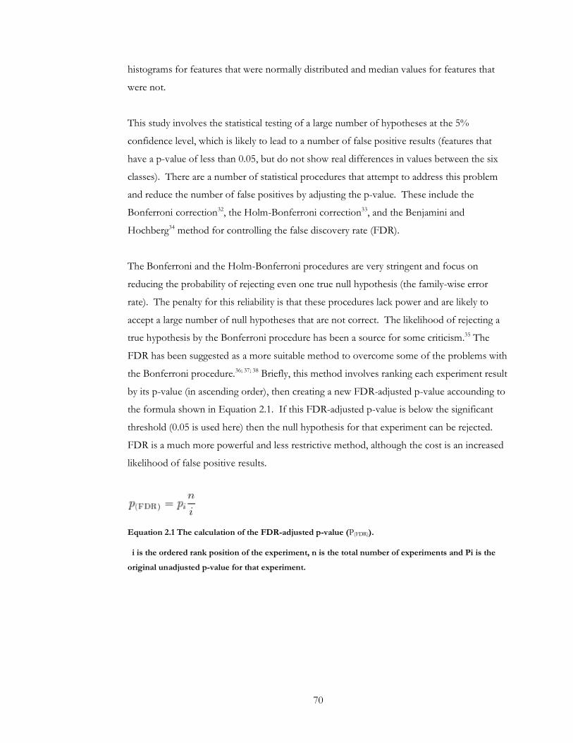
70

histograms for features that were normally distributed and median values for features that

were not.

This study involves the statistical testing of a large number of hypotheses at the 5%

confidence level, which is likely to lead to a number of false positive results (features that

have a p-value of less than 0.05, but do not show real differences in values between the six

classes). There are a number of statistical procedures that attempt to address this problem

and reduce the number of false positives by adjusting the p-value. These include the

Bonferroni correction32, the Holm-Bonferroni correction33, and the Benjamini and

Hochberg34 method for controlling the false discovery rate (FDR).

The Bonferroni and the Holm-Bonferroni procedures are very stringent and focus on

reducing the probability of rejecting even one true null hypothesis (the family-wise error

rate). The penalty for this reliability is that these procedures lack power and are likely to

accept a large number of null hypotheses that are not correct. The likelihood of rejecting a

true hypothesis by the Bonferroni procedure has been a source for some criticism.35 The

FDR has been suggested as a more suitable method to overcome some of the problems with

the Bonferroni procedure.36; 37; 38 Briefly, this method involves ranking each experiment result

by its p-value (in ascending order), then creating a new FDR-adjusted p-value accounding to

the formula shown in Equation 2.1. If this FDR-adjusted p-value is below the significant

threshold (0.05 is used here) then the null hypothesis for that experiment can be rejected.

FDR is a much more powerful and less restrictive method, although the cost is an increased

likelihood of false positive results.

Equation 2.1 The calculation of the FDR-adjusted p-value (P(FDR)).

i is the ordered rank position of the experiment, n is the total number of experiments and Pi is the

original unadjusted p-value for that experiment.

71

In this study, it is appropriate to use a more powerful method in order to give a good

coverage of probable true results, rather than ensure that every result is true at the expense

of many false negatives. The p-values obtained from the hypothesis tests have therefore

been adjusted using the Benjamini and Hochburg method for controlling the false discovery

rate.34

2.2.6 Rotamer Calculations.

In order to calculate the relative flexibilities of aspartic acid and glutamic acid side chains we

used a mean-field program39 developed from earlier work.40 This uses pairwise packing of

rotamers to derive probabilities for rotamers within a fixed sidechain, according to an

allowed van der Waals tolerance in the packing. This tolerance was set at 0.8Å, in keeping

with earlier work.39 Rotamers with zero probability are inaccessible, given the surrounding

mainchain and sidechains. The remaining (non-zero probability) rotamers are then

compared to the number of rotamers in the dictionary to assess the conformational freedom

of a sidechain. These calculations are made for Asp and Glu residues to compare their

flexibility.

72

2.3 Results and Discussion

2.3.1 Dataset and Active Site Definition.

The dataset was created using the criteria outlined in 2.2.1, and contains 294 unique enzymes

from a starting set of 880 (see Figure 2.1 and Table 2.1). Redundancy was culled by

structural similarity, ensuring no two proteins within a class share a domain where at least

one contains the active site, from a common SCOP27 superfamily. This produced a dataset

where the maximum sequence identity between two pairs is 24.1% and the average sequence

identity between enzymes in the set is 11.4%. For each of these enzymes, active site residues

were defined as residues that had at least one atom within 10Å of the centroid calculated

over CSA residues, and at least 5Å2 of solvent accessible surface area. A radius of 10Å

returns almost 95% of the catalytic residues (Figure 2.2), and beyond this the number of

CSA residues returned diminishes rapidly in comparison with other residues. A trade-off is

also required for the solvent accessibility threshold, where we look to exclude buried

residues within the active site radius. A 5Å2 solvent accessible surface area returns over 75%

of CSA residues (Figure 2.2).

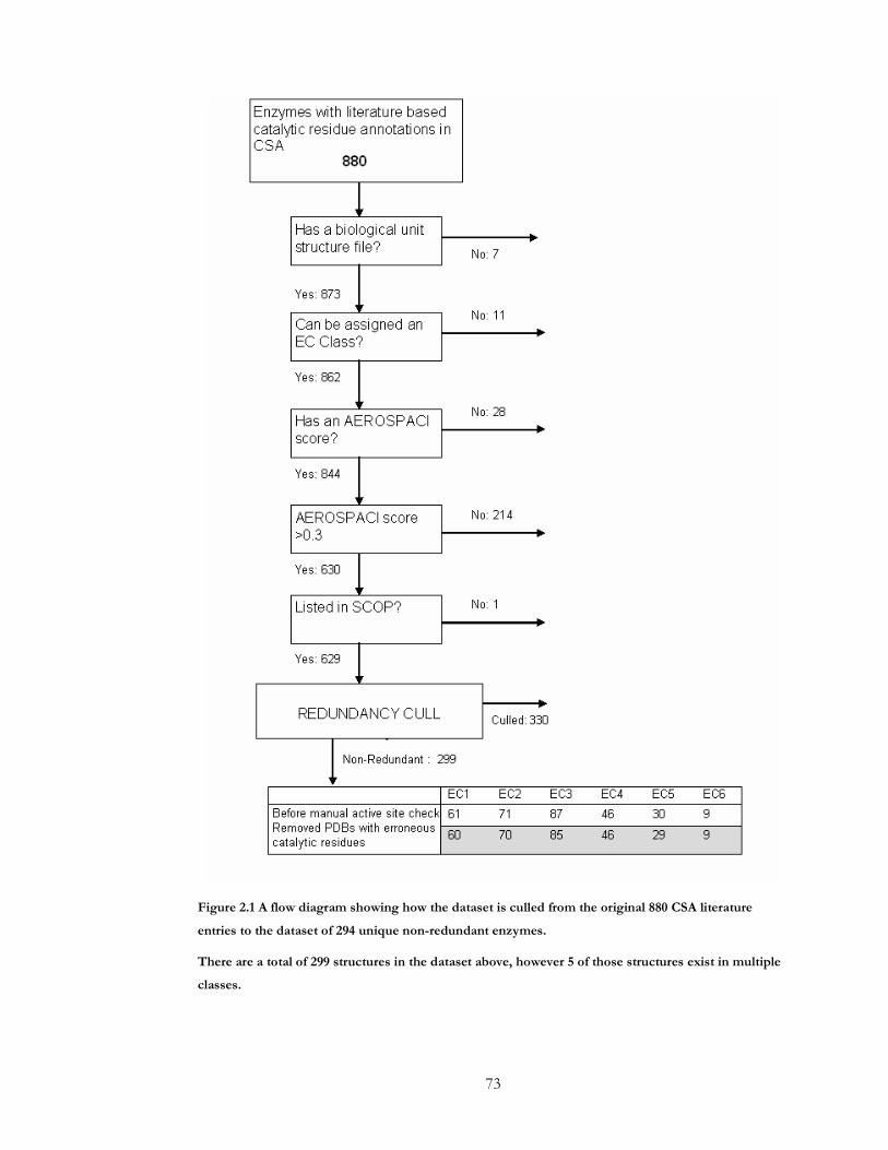
73

Figure 2.1 A flow diagram showing how the dataset is culled from the original 880 CSA literature

entries to the dataset of 294 unique non-redundant enzymes.

There are a total of 299 structures in the dataset above, however 5 of those structures exist in multiple

classes.

74

EC PDB EC PDB EC PDB EC PDB EC PDB EC PDB

1 1a05

1 1a4i

1 1a8q

1 1akd

1 1aop

1 1b5t

1 1bou

1 1bt1

1 1c0k

1 1c9u

1 1d3g

1 1d4a

1 1dhf

1 1do6

1 1dqa

1 1dqs

1 1dve

1 1fnb

1 1g72

1 1g79

1 1gcu

1 1gp1

1 1gpj

1 1gqg

1 1h2r

1 1hfe

1 1i19

1 1jnr

1 1l1d

1 1l1l

1 1l6p

1 1lci

1 1ljl

1 1luc

1 1mrq

1 1ndo

1 1ni4

1 1nid

1 1nir

1 1nml

1 1o04

1 1o9i

1 1oac

1 1opm

1 1qje

1 1qv0

1 1s3i

1 1sox

1 1ti6

1 1vie

1 1vlb

1 1yve

1 2bbk

1 2cpo

1 2jcw

1 2toh

1 3mdd

1 3nos

1 7atj

2 1aj0

2 1al6

2 1bg0

2 1brw

2 1c2t

2 1c3j

2 1cg6

2 1cgk

2 1cqq

2 1cs1

2 1cwy

2 1d0s

2 1d8c

2 1d8d

2 1daa

2 1dqs

2 1e19

2 1e2a

2 1ecf

2 1eh6

2 1ez1

2 1f75

2 1f7l

2 1f8x

2 1foa

2 1g24

2 1g6t

2 1g8f

2 1gpr

2 1h3i

2 1h54

2 1hiv

2 1hka

2 1hxq

2 1hy3

2 1ig8

2 1ir3

2 1iu4

2 1j53

2 1jdw

2 1jm6

2 1jms

2 1k30

2 1lij

2 1mla

2 1moq

2 1nsp

2 1oas

2 1oe8

2 1oj4

2 1onr

2 1oyg

2 1p4n

2 1p4r

2 1pfk

2 1pud

2 1qd1

2 1qpr

2 1rhs

2 1ro7

2 1trk

2 1tys

2 1uam

2 1un1

2 1vid

2 2tdt

2 2tps

2 2ypn

2 3cla

3 135l

3 1a2t

3 1a4i

3 1a79

3 1abr

3 1ah7

3 1ako

3 1apy

3 40391

3 1bol

3 1bp2

3 1bs4

3 1bs9

3 1bwp

3 1cd5

3 1cev

3 1chm

3 1czf

3 1d1q

3 1d2t

3 1d8h

3 1dl2

3 1dmu

3 1dup

3 1e7l

3 1eb6

3 1ef0

3 1eug

3 1fy2

3 1hdh

3 1hzf

3 1itx

3 1j79

3 1j7g

3 1jh6

3 1jhf

3 1js4

3 1k32

3 1k82

3 1kaz

3 1lam

3 1lba

3 1lbu

3 1m21

3 1m6k

3 1mqw

3 1mud

3 1nf9

3 1nln

3 1nlu

3 1nsf

3 1nww

3 1p4r

3 1pa9

3 1pgs

3 1pyl

3 1q3q

3 1qaz

3 1qcn

3 1qd6

3 1qgx

3 1qh5

3 1qq5

3 1qtn

3 1qum

3 1qz9

3 1r16

3 1r4f

3 1s95

3 1ssx

3 1tml

3 1uaq

3 1uf7

3 1v0y

3 1vas

3 2acy

3 40270

3 2eng

3 2nlr

3 2pth

3 3eca

3 5fit

4 1aw8

4 1b66

4 1b93

4 1bfd

4 1bix

4 1c3c

4 1c82

4 1ca2

4 1cl1

4 1db3

4 1dco

4 1dio

4 1dnp

4 1dqs

4 1dw9

4 1dxe

4 1ecm

4 1et0

4 1fgh

4 1fro

4 1fua

4 1hrk

4 1i6p

4 1i7q

4 1mka

4 1mvn

4 1nhx

4 1p1x

4 1pii

4 1pix

4 1ps1

4 1pya

4 1qd1

4 1qj4

4 1qrg

4 1r6w

4 1r76

4 1rbl

4 1ru4

4 1sll

4 1uqr

4 1uro

4 2abk

4 2ahj

4 7odc

5 1bd0

5 1cb7

5 1d6o

5 1dbf

5 1e3v

5 1ecl

5 1ecm

5 1eej

5 1f2v

5 1f6d

5 1jfl

5 1k0w

5 1k4t

5 1lvh

5 1m53

5 1m9c

5 1muc

5 1n20

5 1nn4

5 1o98

5 1otg

5 1p5d

5 1pii

5 1pym

5 1qhf

5 1snn

5 1tph

5 2sqc

5 2xis

6 12as

6 1a4i

6 1dae

6 1gsa

6 1j09

6 1kp2

6 1p3d

6 1qmh

6 1v25

Table 2.1 PDB codes for each enzyme in the dataset.

75

(a)

0

0.1

0.2

0.3

0.4

0.5

0.6

0.7

0.8

0.9

1

0 2 4 6 8 10 12 14 16 18

Distance (Angstroms)

Cum

ula

tive P

erc

enta

ge

(b)

0

20

40

60

80

100

0 5 10 15 20 25 30 35 40Solvent Accessible Surface Area Threshold

(Angstrom2)

Pe

rce

nta

ge

of

CS

A

resid

ue

s c

ove

red

Figure 2.2 The percentage coverage of CSA residues by varying active site criteria thresholds for (a)

surface area and (b) distance from centroid.

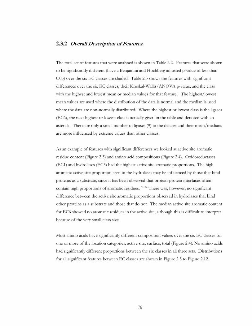
76

2.3.2 Overall Description of Features.

The total set of features that were analysed is shown in Table 2.2. Features that were shown

to be significantly different (have a Benjamini and Hochberg adjusted p-value of less than

0.05) over the six EC classes are shaded. Table 2.3 shows the features with significant

differences over the six EC classes, their Kruskal-Wallis/ANOVA p-value, and the class

with the highest and lowest mean or median values for that feature. The highest/lowest

mean values are used where the distribution of the data is normal and the median is used

where the data are non-normally distributed. Where the highest or lowest class is the ligases

(EC6), the next highest or lowest class is actually given in the table and denoted with an

asterisk. There are only a small number of ligases (9) in the dataset and their mean/medians

are more influenced by extreme values than other classes.

As an example of features with significant differences we looked at active site aromatic

residue content (Figure 2.3) and amino acid compositions (Figure 2.4). Oxidoreductases

(EC1) and hydrolases (EC3) had the highest active site aromatic proportions. The high

aromatic active site proportion seen in the hydrolases may be influenced by those that bind

proteins as a substrate, since it has been observed that protein-protein interfaces often

contain high proportions of aromatic residues. 41; 42 There was, however, no significant

difference between the active site aromatic proportions observed in hydrolases that bind

other proteins as a substrate and those that do not. The median active site aromatic content

for EC6 showed no aromatic residues in the active site, although this is difficult to interpret

because of the very small class size.

Most amino acids have significantly different composition values over the six EC classes for

one or more of the location categories; active site, surface, total (Figure 2.4). No amino acids

had significantly different proportions between the six classes in all three sets. Distributions

for all significant features between EC classes are shown in Figure 2.5 to Figure 2.12.

77

Attribute Structural Features

Active site proportion helix Active site proportion sheet Active site proportion turn Active site proportion non-helix

and non-sheet Active site total B-factor Active site average atomic B-

factor Active site surface area Relative active site surface area Active site non-polar proportion Active site aromatic proportion Active site negative proportion Active-site polar proportion Active site mean hydrophobicity

score Active site positive proportion Active site mean isoelectric point Average total atomic B-factor Relative average active site

atomic B-factor Number of chains Total proportion of helix Total proportion of beta sheet Total proportion of turn Total proportion of non-helix and

non-sheet

Sequence Features

Total negative proportion Total polar proportion Total non-polar proportion Total aromatic proportion Total positive proportion Total mean hydrophobicity score Total mean Isolelectric point Proportion of low complexity

sequence

Size-associated Features

Total surface area Number of residues in the

biological unit Number of chains Length of sequence Total B-factor

Amino Acid Compositions Active site ALA

Active site ARG

Active site ASN

Active site ASP

Active site CYS

Active site GLN

Active site GLU

Active site GLY

Active site HIS

Active site ILE

Active site LEU

Active site LYS

Active site MET

Active site PHE

Active site PRO

Active site SER

Active site THR

Active site TRP

Active site TYR

Active site VAL

Surface ALA

Surface ARG

Surface ASN

Surface ASP

Surface CYS

Surface GLN

Surface GLU

Surface GLY

Surface HIS

Surface ILE

Surface LEU

Surface LYS

Surface MET

Surface PRO

Surface SER

Surface THR

Surface TRP

Surface TYR

Surface VAL

Total ALA

Total ARG

Total ASN

Total ASP

Total CYS

Total GLN

Total GLU

Total GLY

Total HIS

Total ILE

Total LEU

Total LYS

Total MET

Total PHE

Total PRO

Total SER

Total THR

Total TRP

Total TYR

Total VAL

Table 2.2 List of all features calculated for each enzyme.

Features that showed significant differences between the six classes are shaded.

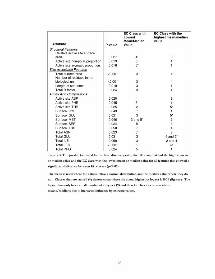
78

Attribute P-value

EC Class with Lowest Mean/Median Value

EC Class with the highest mean/median value

Structural Features

Relative active site surface area 0.027 4* 3

Active site non-polar proportion 0.013 3* 1

Active site aromatic proportion 0.016 5* 1

Size-associated Features

Total surface area <0.001 3 4

Number of residues in the biological unit <0.001 3 4

Length of sequence 0.019 3 1

Total B-factor 0.024 3 4

Amino Acid Compositions Active site ASP 0.020 1 3

Active site PHE 0.045 3* 1

Active site THR 0.025 2 5*

Surface CYS 0.049 5* 1

Surface GLU 0.021 3 5*

Surface MET 0.046 3 and 5* 2

Surface SER 0.024 5 3

Surface TRP 0.050 2* 4

Total ASN 0.023 5* 3

Total GLU 0.031 3 4 and 5*

Total ILE 0.050 3 2 and 4

Total LEU <0.001 1 4*

Total PRO 0.024 5 1

Table 2.3 The p-value (adjusted for the false discovery rate), the EC class that had the highest mean

or median value and the EC class with the lowest mean or median value for all features that showed a

significant difference between EC classes (p<0.05).

The mean is used where the values follow a normal distribution and the median value where they do

not. Classes that are starred (*) denote cases where the actual highest or lowest is EC6 (ligases). The

ligase class only has a small number of enzymes (9) and therefore has less representative

means/medians due to increased influence by extreme values.

79

0.00

0.02

0.04

0.06

0.08

0.10

0.12

EC1 EC2 EC3 EC4 EC5 EC6

Me

dia

n A

rom

atic P

rop

ort

ion

of

Active

Site

Figure 2.3 The median aromatic proportion of the active site for each EC class.

Figure 2.4 Amino acids that showed significant differences between the six EC classes in either the

active site, surface residues or the total protein.

A shaded box indicates a false discovery rate adjusted p-value of less than 0.05.

80

0.00

0.05

0.10

0.15

0.20

0.25

0.30

0.35

0.40

0.45

0.50

Active Site Non-PolarProportion

Active Site AromaticProportion

Pro

port

ion o

f active s

ite

Figure 2.5 The median value of significantly different charge-related features for each EC class.

0.000

0.005

0.010

0.015

0.020

0.025

0.030

0.035

0.040

0.045

0.050

Relative Active Site Surface Area

Pro

po

rtio

n o

f active s

ite

Figure 2.6 The median proportion of the total surface area that belongs to the active site for each EC

class.

0

100

200

300

400

500

600

700

800

Sequence Length Number of Residues in theBiological Unit

Num

ber

of

Resid

ues

Figure 2.7 The median value of significantly different size-related features for each EC class.

Key

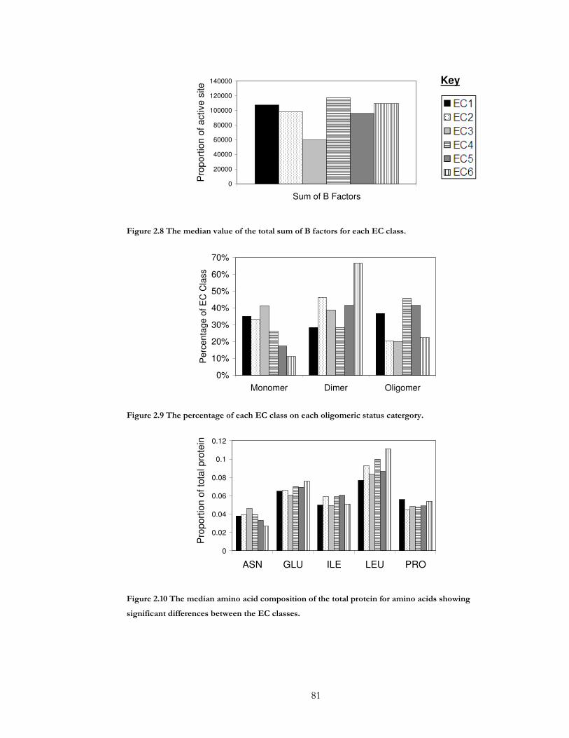
81

0

20000

40000

60000

80000

100000

120000

140000

Sum of B FactorsP

ropo

rtio

n o

f active s

ite

Figure 2.8 The median value of the total sum of B factors for each EC class.

0%

10%

20%

30%

40%

50%

60%

70%

Monomer Dimer Oligomer

Pe

rce

nta

ge

of E

C C

lass

Figure 2.9 The percentage of each EC class on each oligomeric status catergory.

0

0.02

0.04

0.06

0.08

0.1

0.12

ASN GLU ILE LEU PRO

Pro

port

ion

of to

tal pro

tein

Figure 2.10 The median amino acid composition of the total protein for amino acids showing

significant differences between the EC classes.

Key

82

0

0.02

0.04

0.06

0.08

0.1

0.12

CYS GLU MET SER TRPP

rop

ort

ion

of

Surf

ace

Figure 2.11 The median amino acid composition of the protein surface for amino acids showing

significant differences between the EC classes

0.00

0.02

0.04

0.06

0.08

0.10

0.12

0.14

ASP PHE THR

Pro

po

rtio

n o

f A

cti

ve

Sit

e

Figure 2.12 The median amino acid composition of the active site for amino acids showing significant

differences between the EC classes

Key

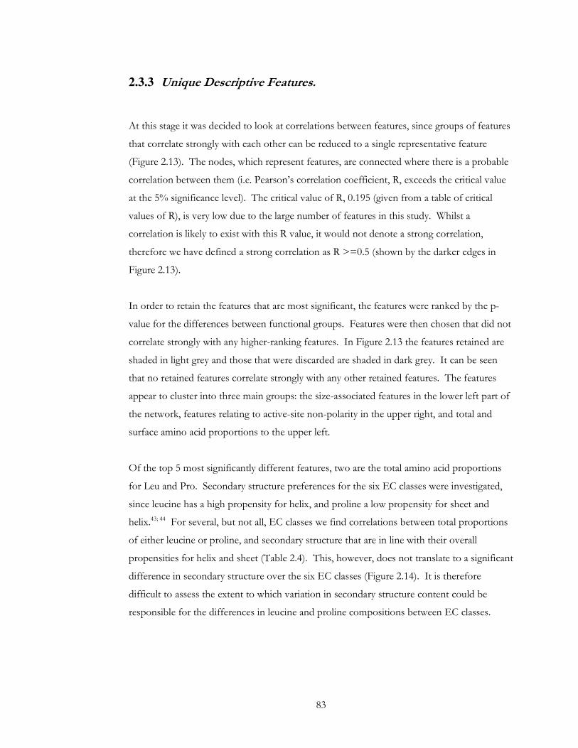
83

2.3.3 Unique Descriptive Features.

At this stage it was decided to look at correlations between features, since groups of features

that correlate strongly with each other can be reduced to a single representative feature

(Figure 2.13). The nodes, which represent features, are connected where there is a probable

correlation between them (i.e. Pearson’s correlation coefficient, R, exceeds the critical value

at the 5% significance level). The critical value of R, 0.195 (given from a table of critical

values of R), is very low due to the large number of features in this study. Whilst a

correlation is likely to exist with this R value, it would not denote a strong correlation,

therefore we have defined a strong correlation as R >=0.5 (shown by the darker edges in

Figure 2.13).

In order to retain the features that are most significant, the features were ranked by the p-

value for the differences between functional groups. Features were then chosen that did not

correlate strongly with any higher-ranking features. In Figure 2.13 the features retained are

shaded in light grey and those that were discarded are shaded in dark grey. It can be seen

that no retained features correlate strongly with any other retained features. The features

appear to cluster into three main groups: the size-associated features in the lower left part of

the network, features relating to active-site non-polarity in the upper right, and total and

surface amino acid proportions to the upper left.

Of the top 5 most significantly different features, two are the total amino acid proportions

for Leu and Pro. Secondary structure preferences for the six EC classes were investigated,

since leucine has a high propensity for helix, and proline a low propensity for sheet and

helix.43; 44 For several, but not all, EC classes we find correlations between total proportions

of either leucine or proline, and secondary structure that are in line with their overall

propensities for helix and sheet (Table 2.4). This, however, does not translate to a significant

difference in secondary structure over the six EC classes (Figure 2.14). It is therefore

difficult to assess the extent to which variation in secondary structure content could be

responsible for the differences in leucine and proline compositions between EC classes.

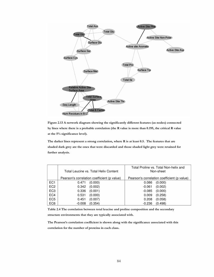
84

Figure 2.13 A network diagram showing the significantly different features (as nodes) connected

by lines where there is a probable correlation (the R value is more than 0.195, the critical R value

at the 5% significance level).

The darker lines represent a strong correlation, where R is at least 0.5. The features that are

shaded dark grey are the ones that were discarded and those shaded light grey were retained for

further analysis.

Total Leucine vs. Total Helix Content Total Proline vs. Total Non-helix and

Non-sheet

Pearson's correlation coefficient (p value)

Pearson's correlation coefficient (p value)

EC1 0.471 (0.000) 0.086 (0.000)

EC2 0.342 (0.002) -0.061 (0.002)

EC3 0.336 (0.001) -0.085 (0.000)

EC4 0.531 (0.000) 0.009 (0.258)

EC5 0.451 (0.007) 0.208 (0.058)

EC6 -0.008 (0.354) -0.236 (0.498)

Table 2.4 The correlation between total leucine and proline composition and the secondary

structure environments that they are typically associated with.

The Pearson’s correlation coefficient is shown along with the significance associated with this

correlation for the number of proteins in each class.

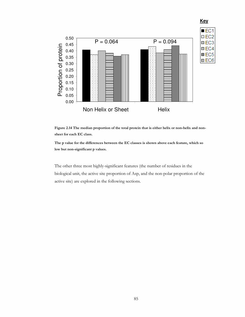
85

0.00

0.05

0.10

0.15

0.20

0.25

0.30

0.35

0.40

0.45

0.50

Non Helix or Sheet Helix

Pro

po

rtio

n o

f p

rote

in

P = 0.064 P = 0.094

Figure 2.14 The median proportion of the total protein that is either helix or non-helix and non-

sheet for each EC class.

The p value for the differences between the EC classes is shown above each feature, which so

low but non-significant p values.

The other three most highly-significant features (the number of residues in the

biological unit, the active site proportion of Asp, and the non-polar proportion of the

active site) are explored in the following sections.

Key

86

2.3.4 Differences in Structure Sizes due to Different Oligomeric

State Preferences

All but one of the size-related features were found to show significant differences

between the six classes. These features correlated strongly with each other, apart from

sequence length (see Figure 2.13), and the number of residues in the biological unit was

chosen as the representative feature for further detailed analysis. Figure 2.7 shows the

differences in sequence length and the number of residues in the biological unit PDB

file. The sequence length is the number of residues in the sequence of each distinct

chain in the PDB file (duplicate chains are not counted twice), whereas the number of

residues in the biological unit counts residues in duplicate chains. The number of

residues in the biological unit is on average larger than the number of residues in the

sequence due to the oligomerisation of protein chains in biologically functional units.

It could be expected that since the oxidoreductases have the largest sequence lengths,

they would also have the largest number of residues in the biological unit. The lyases,

however, actually have the largest number of residues in the biological unit, due to a

preference for higher order oligomers compared to oxidoreductases (Figure 2.9).

The hydrolases (EC3) and lyases (EC4) were the only classes that had significantly

different proportions of monomers, dimers and oligomers to the other classes (p-value

= 0.001 and 0.024, respectively). Lyases have the largest percentages of enzymes that

form oligomers and the lowest proportion of enzymes that form monomers, whereas

hydrolases tend to exist as monomers and have the lowest proportion of oligomers of

all the classes (see Figure 2.9).

Generally, hydrolases have the simplest task of the six classes since hydrolysis is usually

an energetically favourable reaction and therefore they may not require the

complication of forming higher order oligomers. There are also other functional

advantages to enzymes existing as monomers, for example stability at low

concentrations and rapid diffusion. Rapid diffusion is particularly relevant for

extracellular hydrolases, for passage through the cell membranes to their site of

action.24 Subcellular location annotation is only available for 21 of the 85 hydrolases

(see Table 2.5). Two of these hydrolases are annotated as extracellular (secreted), both

87

of which are monomers. All 9 extracellular enzymes in the total set are monomeric,

which suggests that extracellular enzymes prefer to exist as monomers. There is,

however, not enough information to reveal the influence of extracellular location on

the preference of EC3 to exist as a monomer.

Conversely, the lyases have the highest proportion of oligomers and the lowest

proportion of monomers (see Figure 2.9). There are stability benefits to proteins

forming large complexes due an increase in the number of internal interactions

enabling a lower surface to volume ratio. Furthermore, multimeric complexes,

particularly homo-oligomers, are a genetically economical way of producing large

proteins and the subunit based assembly allows for an extra step in error control

whereby defective subunits can be discarded.45 One functional advantage of

multimeric enzymes is the opportunity for increased catalytic control by cooperativity

between active sites in individual subunits or by allosteric action between the subunits.

For the multimeric protein structures in our dataset, we assessed whether the active site

of the enzyme was close to or at a subunit boundary as a means of estimating how

many of the enzymes may have their action regulated by the formation of the

multimeric complex. If the active site amino acids (defined in 2.2.2) from a single site

in an enzyme come from separate chains then the active site is defined as ‘shared’. If

they are all from the same chain then the site is defined as ‘single’.

In all EC classes a larger proportion of dimers have single active sites than shared

active sites (60% have a single active site, whereas 40% have a shared active site). This

is opposite to oligomers with three or more chains, which are more likely to have

shared active sites than single (40% have a single active site, whereas 60% have a

shared active site). When broken down into EC class it is evident that the class with

the largest number of oligomers (EC4) is also the class that has the largest percentage

of oligomers having shared active sites (see Figure 2.15). This suggests that the over-

representation of oligomers in this class can be attributed to the formation of the active

site by multiple subunits.

88

Subcellular Location EC1 EC2 EC3 EC4 EC5 EC6 All

Cytoplasm 8 (30.77%) 15 (60.00%) 12 (57.14%) 9 (64.29%) 6 (75.00%) 7 (100.00%) 57 (56.44%) Mitochondria 4 (15.38%) 4 (16.00%) 0 (0.00%) 2 (14.29%) 0 (0.00%) 0 (0.00%) 10 (9.90%)

Secreted 4 (15.38%) 1 (4.00%) 2 (9.52%) 2 (14.29%) 0 (0.00%) 0 (0.00%) 9 (8.91%)

Periplasm 5 (19.23%) 0 (0.00%) 1 (4.76%) 0 (0.00%) 1 (12.50%) 0 (0.00%) 7 (6.93%)

Nucleus 0 (0.00%) 2 (8.00%) 3 (14.29%) 1 (7.14%) 0 (0.00%) 0 (0.00%) 6 (5.94%)

Membrane 2 (7.69%) 1 (4.00%) 1 (4.76%) 0 (0.00%) 1 (12.50%) 0 (0.00%) 5 (4.95%)

Peroxisome 2 (7.69%) 0 (0.00%) 0 (0.00%) 0 (0.00%) 0 (0.00%) 0 (0.00%) 2 (1.98%)

Chloroplast 1 (3.85%) 1 (4.00%) 0 (0.00%) 0 (0.00%) 0 (0.00%) 0 (0.00%) 2 (1.98%)

Endoplasmic Reticulum 0 (0.00%) 0 (0.00%) 1 (4.76%) 0 (0.00%) 0 (0.00%) 0 (0.00%) 1 (0.99%)

Lysosome 0 (0.00%) 0 (0.00%) 1 (4.76%) 0 (0.00%) 0 (0.00%) 0 (0.00%) 1 (0.99%)

Golgi Apparatus 0 (0.00%) 1 (4.00%) 0 (0.00%) 0 (0.00%) 0 (0.00%) 0 (0.00%) 1 (0.99%)

26 (100%) 25 (100%) 21 (100%) 14 (100%) 8 (100%) 7 (100%) 101 (100%)

Table 2.5 Subcellular location annotation (where available) for each EC class.

The percentages are based on the number in the class with subcellular location annotation. Approximately a third of the total set (101 out of 294) have subcellular

location information.

0%

10%

20%

30%

40%

50%

60%

70%

80%

90%

100%


Pe

rcenta

ge o

f O

ligom

ers

in the

C

lass

Single

Shared

Figure 2.15 The percentage of oligomers that have single sub-unit or shared sub-unit active sites

in each class.

The hydrolases, which have the highest monomer and lowest oligomer proportions, is

the only class where the oligomers prefer to have single subunit active sites (excluding

EC6, which only has 2 oligomers). In contrast to the lyases, when hydrolases do form

oligomers it does not appear to be for functional reasons associated with their active

site and may be in an attempt to overcome the stability disadvantages of small proteins

(hydrolases have the smallest average number of residues in the biological unit).

2.3.4.1 Lyases and Hydrolases in Metabolic Networks

Metabolic networks represent how enzymes are linked to each other via their reactions.

Enzymes in the network that are highly connected to other enzymes (involved in

catalytic reactions with multiple different enzymes) or are at critical points in the

network through which many reaction pathways flow, are important to the stability of

the network. These enzymes therefore have to be highly regulated and their catalytic

rate tightly controlled. Cooperativity and allosteric interaction of active sites can be

used as a further level of control of enzyme action and therefore enzymes whose active

sites communicate in this way may be found at highly regulated points in a metabolic

network.

90

The Pathway Hunter tool46 holds information about metabolic networks for a given

organism, with the nodes representing enzymes or metabolites and the connections

representing their reactions. It also gives statistical and quantative information relating

to the importance of the enzymes in the networks. Traditionally, important enzymes in

a metabolic network would be identified by the number of connections to other

enzymes. Raman and Schomburg, however, proposed other measures of importance in

networks, namely choke points and load points.47 Load points are a measure of the

enzyme’s importance in a network. They are calculated by dividing the number of

metabolic pathways that pass through a node (the shortest route between two

metabolites is assumed) by the number of incoming or outgoing connections. This is

then divided by the average load value for the whole network. Choke points are used

to identify biochemical lethality in the network, where a choke point is defined as an

enzyme that uniquely produces or consumes a particular metabolite.

The distribution of enzymes over the six EC classes in a list of enzymes defined as

choke points in the Saccharomyces cerevisiae metabolic network was calculated using the

Pathway Hunter tool. The expected number of enzymes in each EC class was

calculated using the background distribution from all enzymes in the Saccharomyces

cerevisiae genome. The observed number of enzymes in each class in sets of defined

nodes (either choke points or load points) was divided by the expected number. The

class with the highest percentage of oligomers, the lyases (EC4), was significantly

overrepresented in the list of choke points (Figure 2.16). Similarly, the class with the

lowest percentage of oligomers, the hydrolases (EC3) was significantly

underrepresented. These results were even more marked when only considering the

top 50% of choke points with the highest incoming load value. This was also repeated

for the 25% most loaded (incoming and outgoing) enzymes and similar results were

obtained (Figure 2.17). We suggest that the more important enzymes in a network are

more likely to be oligomeric.

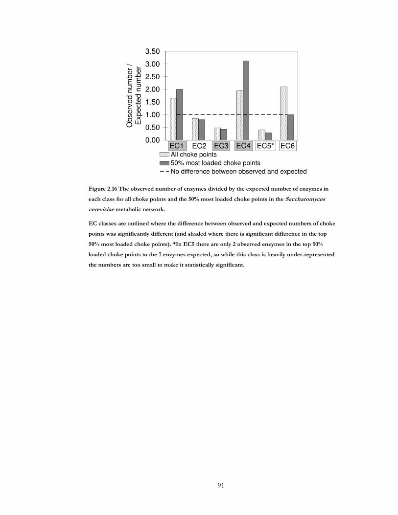
91

0.00

0.50

1.00

1.50

2.00

2.50

3.00

3.50

1 2 3 4 5 6

Ob

serv

ed n

um

ber

/E

xpecte

d n

um

ber

All choke points

50% most loaded choke points

No difference between observed and expected

EC1 EC2 EC3 EC4 EC5* EC6

Figure 2.16 The observed number of enzymes divided by the expected number of enzymes in

each class for all choke points and the 50% most loaded choke points in the Saccharomyces

cerevisiae metabolic network.

EC classes are outlined where the difference between observed and expected numbers of choke

points was significantly different (and shaded where there is significant difference in the top

50% most loaded choke points). *In EC5 there are only 2 observed enzymes in the top 50%

loaded choke points to the 7 enzymes expected, so while this class is heavily under-represented

the numbers are too small to make it statistically significant.

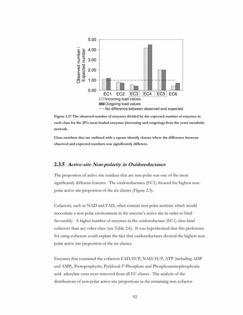
92

0.00

1.00

2.00

3.00

4.00

5.00

1 2 3 4 5 6

Obse

rved

nu

mb

er

/E

xp

ecte

d n

um

be

r

Incoming load values

Outgoing load values

No difference between observed and expected


Figure 2.17 The observed number of enzymes divided by the expected number of enzymes in

each class for the 25% most loaded enzymes (incoming and outgoing) from the yeast metabolic

network.

Class numbers that are outlined with a square identify classes where the difference between

observed and expected numbers was significantly different.

2.3.5 Active-site Non-polarity in Oxidoreductases

The proportion of active site residues that are non-polar was one of the most

significantly different features. The oxidoreductases (EC1) showed the highest non-

polar active site proportion of the six classes (Figure 2.5).

Cofactors, such as NAD and FAD, often contain non-polar sections which would

necessitate a non-polar environment in the enzyme’s active site in order to bind

favourably. A higher number of enzymes in the oxidoreductase (EC1) class bind

cofactors than any other class (see Table 2.6). It was hypothesised that this preference

for using cofactors could explain the fact that oxidoreductases showed the highest non-

polar active site proportion of the six classes.

Enzymes that contained the cofactors FAD/H/P, NAD/H/P, ATP (including ADP

and AMP), Protoporphyrin, Pyridoxal-5'-Phosphate and Phosphoaminophosphonic

acid- adenylate ester were removed from all EC classes. The analysis of the

distributions of non-polar active site proportions in the remaining non cofactor-

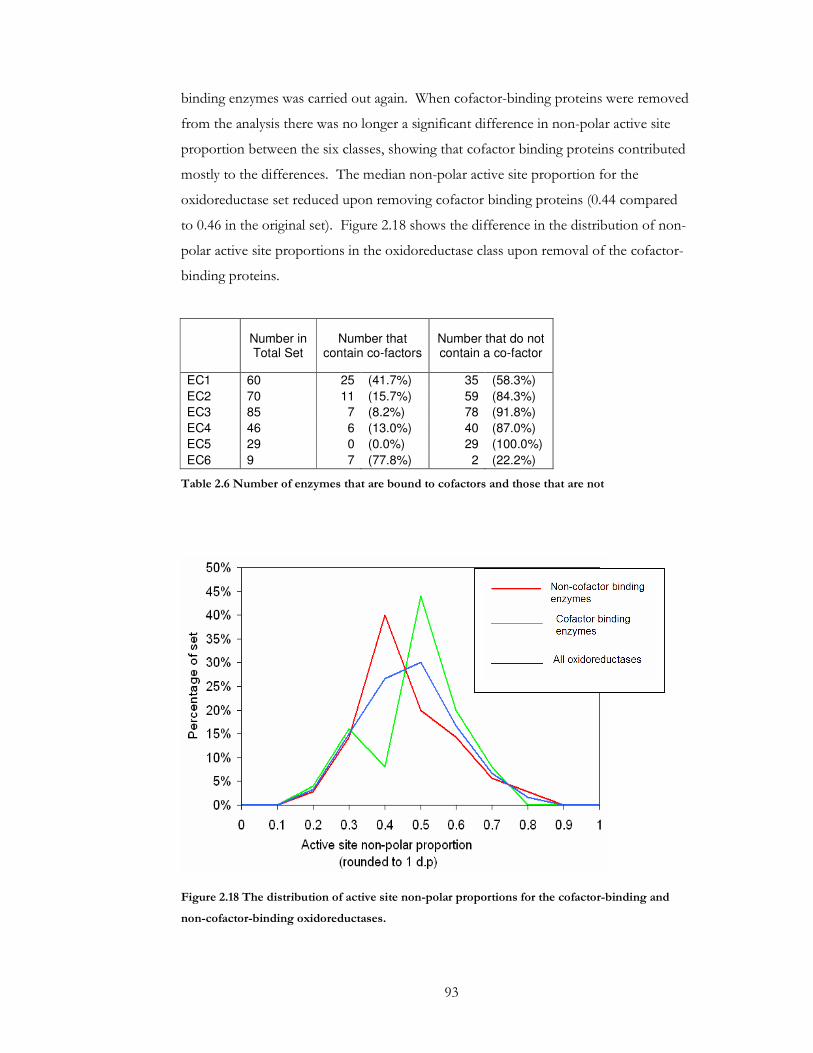
93

binding enzymes was carried out again. When cofactor-binding proteins were removed

from the analysis there was no longer a significant difference in non-polar active site

proportion between the six classes, showing that cofactor binding proteins contributed

mostly to the differences. The median non-polar active site proportion for the

oxidoreductase set reduced upon removing cofactor binding proteins (0.44 compared

to 0.46 in the original set). Figure 2.18 shows the difference in the distribution of non-

polar active site proportions in the oxidoreductase class upon removal of the cofactor-

binding proteins.

Number in Total Set

Number that contain co-factors

Number that do not contain a co-factor

EC1 60 25 (41.7%) 35 (58.3%)

EC2 70 11 (15.7%) 59 (84.3%)

EC3 85 7 (8.2%) 78 (91.8%)

EC4 46 6 (13.0%) 40 (87.0%)

EC5 29 0 (0.0%) 29 (100.0%)

EC6 9 7 (77.8%) 2 (22.2%)

Table 2.6 Number of enzymes that are bound to cofactors and those that are not

Figure 2.18 The distribution of active site non-polar proportions for the cofactor-binding and

non-cofactor-binding oxidoreductases.

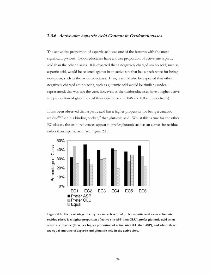
94

2.3.6 Active-site Aspartic Acid Content in Oxidoreductases

The active site proportion of aspartic acid was one of the features with the most

significant p-value. Oxidoreductases have a lower proportion of active site aspartic

acid than the other classes. It is expected that a negatively charged amino acid, such as

aspartic acid, would be selected against in an active site that has a preference for being

non-polar, such as the oxidoreductases. If so, it would also be expected that other

negatively charged amino acids, such as glutamic acid would be similarly under-

represented; this was not the case, however, as the oxidoreductases have a higher active

site proportion of glutamic acid than aspartic acid (0.046 and 0.039, respectively).

It has been observed that aspartic acid has a higher propensity for being a catalytic

residue18; 48 or in a binding pocket,49 than glutamic acid. Whilst this is true for the other

EC classes, the oxidoreductases appear to prefer glutamic acid as an active site residue,

rather than aspartic acid (see Figure 2.19).

0%

10%

20%

30%

40%

50%


Perc

enta

ge o

f C

lass

Prefer ASPPrefer GLUEqual

Figure 2.19 The percentage of enzymes in each set that prefer aspartic acid as an active site

residue (there is a higher proportion of active site ASP than GLU), prefer glutamic acid as an

active site residue (there is a higher proportion of active site GLU than ASP), and where there

are equal amounts of aspartic and glutamic acid in the active sites.

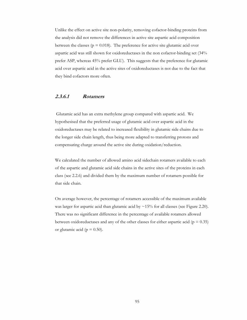
95

Unlike the effect on active site non-polarity, removing cofactor-binding proteins from

the analysis did not remove the differences in active site aspartic acid composition

between the classes (p = 0.018). The preference for active site glutamic acid over

aspartic acid was still shown for oxidoreductases in the non cofactor-binding set (34%

prefer ASP, whereas 45% prefer GLU). This suggests that the preference for glutamic

acid over aspartic acid in the active sites of oxidoreductases is not due to the fact that

they bind cofactors more often.

2.3.6.1 Rotamers

Glutamic acid has an extra methylene group compared with aspartic acid. We

hypothesised that the preferred usage of glutamic acid over aspartic acid in the

oxidoreductases may be related to increased flexibility in glutamic side chains due to

the longer side chain length, thus being more adapted to transferring protons and

compensating charge around the active site during oxidation/reduction.

We calculated the number of allowed amino acid sidechain rotamers available to each

of the aspartic and glutamic acid side chains in the active sites of the proteins in each

class (see 2.2.6) and divided them by the maximum number of rotamers possible for

that side chain.

On average however, the percentage of rotamers accessible of the maximum available

was larger for aspartic acid than glutamic acid by ~15% for all classes (see Figure 2.20).

There was no significant difference in the percentage of available rotamers allowed

between oxidoreductases and any of the other classes for either aspartic acid (p = 0.35)

or glutamic acid (p = 0.50).

96

0%

10%

20%

30%

40%

50%

60%

70%

80%


Perc

enta

ge o

f th

e m

axim

um

allo

wed

ro

tam

ers

that

are

accepta

ble

ASP

GLU

Figure 2.20 The percentage of accessible rotamers available to all active site ASP and GLU in

each class.

2.3.6.2 Hydrogen Bonding

Hydrogen bonds were calculated using HBPLUS50 for all aspartic acid residues and

glutamic acid residues in each structure that contained either an aspartic or glutamic

acid in their active site. The average number of hydrogen bonds per active site and

non active site aspartic and glutamic acid are shown in Table 2.7.

The average number of hydrogen bonds for each glutamic acid residue was larger for

active site residues than non-active site residues in each EC class, whereas there is no

significant difference between the average number of hydrogen bonds for active site

and non active site aspartic acid residues.

97

EC1 is the only class for which the average number of hydrogen bonds per active site

glutamic acid is significantly larger than average number of hydrogen bonds per active

site aspartic acid. This class also has the largest average number of hydrogen bonds per

active site glutamic acid of all the six classes. This may be related to the fact that

oxidoreductases are the only class to prefer glutamic acid over aspartic acid in their

active site. Figure 2.1 shows the difference in distribution of number of hydrogen

bonds per active site residue between aspartic acid and glutamic acid in EC1.

All Active site Non active site

EC

Average hydrogen bonds per ASP

Average hydrogen bonds per GLU





1 2.95 2.72 2.72 3.32 2.95 2.70

2 2.84 2.52 2.88 2.85 2.84 2.51

3 2.97 2.55 2.85 2.92 2.97 2.53

4 2.93 2.57 2.62 2.96 2.94 2.55

5 2.68 2.54 2.95 3.03 2.67 2.52

6 2.99 2.56 2.20 2.88 3.06 2.54

Table 2.7 Average number of hydrogen bonds per aspartic acid/glutamic acid split by active-

site residues and non-active-site residues

0%

5%

10%

15%

20%

1 2 3 4 5 6 7 8 9Number of hydrogen bonds per

residue

Perc

enta

ge o

f active s

ite

AS

P &

GLU

in E

C1

Asp

Glu

Figure 2.21 The underlying distribution for the number of hydrogen bonds per ASP or GLU in

the active site for EC1.

98

2.4 Conclusions

Previous studies of the properties of enzyme active site residues,18; 49 have focused on

the difference between catalytic or binding pocket residues and other residues, rather

than between active sites of different functions. Other studies14; 15 have shown

differences in structural properties between proteins of different functions, though

these have tended to focus on specific individual functions against all other functions.

To our knowledge, this is the first systematic study of the differences in sequence and

structural features of the six main functional classes of non-evolutionarily related

enzymes and their active sites.

Previous work by Dobson and Doig,16 has shown that global structural features can be

used to distinguish between enzyme functions. The use of non-transparent machine

learning methods in this work made the interpretation of the relationships between

these features and the different functions difficult. Here, we systematically evaluate the

relationship between global attributes and the six main functional classes, as well as

adding active site features. We find numerous features show significant differences

between proteins in the six main classes, and have investigated the relationship

between the most significantly different features and enzyme function, following a

clustering procedure.

Here it is shown that an enzyme’s oligomerisation status differs between the six EC

classes with hydrolases having a significantly larger proportion of monomers and a

lower proportion of oligomers than the other classes. Lyases have a significantly

higher proportion of enzymes existing as oligomers (3 or more chains). The lyases also

have the highest number of oligomers that have active sites located at, or very close to,

subunit interfaces. It was hypothesised that lyases may prefer to have structures that

allow communication between active sites in order to achieve a higher level of

regulation. This was supported by evidence that lyases are indeed over-represented in

comparison to the other classes in the most biochemically important points in the yeast

metabolic network. Conversely, the hydrolases, which contained the lowest proportion

of oligomers, were significantly underrepresented in these highly controlled network

positions.

99

The proportion of the enzyme’s active site that is non-polar differed significantly

between the functional classes. The oxidoreductases showed the highest active site

non-polar proportion, which was found to be related to the oxidoreductase’s

preference for binding cofactors. It may be advantageous for enzymes that bind

cofactors to have non-polar active sites in order to accommodate the non-polar regions

contained in the cofactors. Enzymes that were found to bind cofactors in their crystal

structure were removed from the analyses and a significant difference was no longer

found in the active site non-polarity between the functional classes.

Oxidoreductases also showed unusually low Asp usage in their active sites. This is

unrelated to cofactor-binding, as differences in active site Asp proportions remain

when the cofactor-binding enzymes are removed from the analysis. Indeed, the under-

representation of Asp residues in oxidoreductase active sites was not mirrored by the

other negatively charged residue, Glu. Despite it being reported that Asp is more often

found as an active site residue than Glu,18; 48;49 the oxidoreductases exhibit a preference

for Glu over Asp in their active sites. The other EC classes show the expected

preference for Asp over Glu. We have shown that this possibly relates to active site

glutamic acid residues making a significantly higher average number of hydrogen bonds

in oxidoreductases than any other class. Oxidoreductase was also the only class in

which the active site glutamic acid made significantly more hydrogen bonds per residue

than the active site aspartic acid residues. A study of sidechain rotameric freedom

showed little difference between Asp and Glu, but how rotamers are related to

hydrogen bonding networks remains to be established. An obvious feature of

oxidoreductases is that they require electron transfer, often compensated by proton

movement. It is possible that the preference for Glu over Asp relates to an adaptation

related to charge transfer, but in a complex manner that remains to be established.

Indeed, subsequent to this work being published, a survey of the information

contained in the catalytic mechanism database, MACiE9; 51, revealed that Glu is used as

a catalytic residue in oxidoreductases more often than Asp48. It was also noted that the

most common annotated mechanistic function of catalytic residues in oxidoreductases

is “proton shuffling” and that Glu has a much higher likelihood of acting as a general

100

acid/base and taking part in proton shuffling in oxidoreductases (and all other classes

apart from the ligases) than Asp.

It is discussed here how three of the significantly different features directly may relate

to the enzyme’s catalytic action. There may however be complications in relating every

feature directly to a common function for the top EC class due to the way that the

enzymes are classified in the EC classification. EC classifies enzymes by the overall

reaction which they catalyse, hence enzymes that use similar mechanistic steps to

catalyse different reactions, will be grouped in different classes. Mandalate racemase

(EC5), galactonate dehydratase (EC4) and carboxyphosphonoenolpyruvate synthase

(EC2) have diverse overall reactions, and as such are classified in different EC classes.

They do however, share a common mechanistic step; abstracting the α-proton of a

carboxylic acid to form an enolic intermediate.52 Similarly, enzymes in the same top

EC class are unlikely to share the same complete mechanism. It has been shown that

little mechanistic similarity is common within enzymes at the class level of the EC

hierarchy.53

Structural features, particularly of the active site, may relate to these mechanistic steps

rather than the overall reaction. If a structural feature does relate to a common step

involved in the catalysis of diverse overall reactions, grouping enzymes by their top EC

class would not reveal significant differences in this feature. It therefore does not

mean that features that lack significant differences between EC classes do not relate to

the enzyme’s function.

This systematic study of novel differences in structural features between enzyme

function sheds new light on the relationship between protein structure and function.

This may aid the development of further methods to predict protein function from

structure without the use of alignments and in enzyme design.

101

2.5 References

1. Bray, T., Doig, A. J. & Warwicker, J. (2009). Sequence and structural features of enzymes and their active sites by EC class. J Mol Biol 386, 1423-36.

2. Berman, H. M., Westbrook, J., Feng, Z., Gilliland, G., Bhat, T. N., Weissig, H., Shindyalov, I. N. & Bourne, P. E. (2000). The Protein Data Bank. Nucleic Acids Res 28, 235-42.

3. Bork, P. & Koonin, E. V. (1998). Predicting functions from protein sequences--where are the bottlenecks? Nat Genet 18, 313-8.

4. Iliopoulos, I., Tsoka, S., Andrade, M. A., Enright, A. J., Carroll, M., Poullet, P., Promponas, V., Liakopoulos, T., Palaios, G., Pasquier, C., Hamodrakas, S., Tamames, J., Yagnik, A. T., Tramontano, A., Devos, D., Blaschke, C., Valencia, A., Brett, D., Martin, D., Leroy, C., Rigoutsos, I., Sander, C. & Ouzounis, C. A. (2003). Evaluation of annotation strategies using an entire genome sequence. Bioinformatics 19, 717-26.

5. Barrett, A. J., Canter, C. R., Liebecq, C., Moss, G. P., Saenger, W., Sharon, N., Tipton, K. F., Vnetianer, P. & Vliegenthart, V. F. G. (1992). Enzyme Nomenclature, Academic Press, San Diego, CA.

6. Barthelmes, J., Ebeling, C., Chang, A., Schomburg, I. & Schomburg, D. (2007). BRENDA, AMENDA and FRENDA: the enzyme information system in 2007. Nucleic Acids Res 35, D511-4.

7. Bairoch, A. (2000). The ENZYME database in 2000. Nucleic Acids Res 28, 304-5.

8. Pegg, S. C., Brown, S. D., Ojha, S., Seffernick, J., Meng, E. C., Morris, J. H., Chang, P. J., Huang, C. C., Ferrin, T. E. & Babbitt, P. C. (2006). Leveraging enzyme structure-function relationships for functional inference and experimental design: the structure-function linkage database. Biochemistry 45, 2545-55.

9. Holliday, G. L., Almonacid, D. E., Bartlett, G. J., O'Boyle, N. M., Torrance, J. W., Murray-Rust, P., Mitchell, J. B. & Thornton, J. M. (2007). MACiE (Mechanism, Annotation and Classification in Enzymes): novel tools for searching catalytic mechanisms. Nucleic Acids Res 35, D515-20.

10. Pearl, F. M., Bennett, C. F., Bray, J. E., Harrison, A. P., Martin, N., Shepherd, A., Sillitoe, I., Thornton, J. & Orengo, C. A. (2003). The CATH database: an extended protein family resource for structural and functional genomics. Nucleic Acids Res 31, 452-5.

11. Todd, A. E., Orengo, C. A. & Thornton, J. M. (2001). Evolution of function in protein superfamilies, from a structural perspective. J Mol Biol 307, 1113-43.

12. George, R. A., Spriggs, R. V., Thornton, J. M., Al-Lazikani, B. & Swindells, M. B. (2004). SCOPEC: a database of protein catalytic domains. Bioinformatics 20 Suppl 1, i130-6.

13. Hegyi, H. & Gerstein, M. (1999). The relationship between protein structure and function: a comprehensive survey with application to the yeast genome. J Mol Biol 288, 147-64.

14. Stawiski, E. W., Baucom, A. E., Lohr, S. C. & Gregoret, L. M. (2000). Predicting protein function from structure: unique structural features of proteases. Proc Natl Acad Sci U S A 97, 3954-8.

102

15. Stawiski, E. W., Mandel-Gutfreund, Y., Lowenthal, A. C. & Gregoret, L. M. (2002). Progress in predicting protein function from structure: unique features of O-glycosidases. Pac Symp Biocomput, 637-48.

16. Dobson, P. D. & Doig, A. J. (2005). Predicting enzyme class from protein structure without alignments. J Mol Biol 345, 187-99.

17. Laskowski, R. A., Watson, J. D. & Thornton, J. M. (2005). Protein function prediction using local 3D templates. J Mol Biol 351, 614-26.

18. Bartlett, G. J., Porter, C. T., Borkakoti, N. & Thornton, J. M. (2002). Analysis of catalytic residues in enzyme active sites. J Mol Biol 324, 105-21.

19. Amitai, G., Shemesh, A., Sitbon, E., Shklar, M., Netanely, D., Venger, I. & Pietrokovski, S. (2004). Network analysis of protein structures identifies functional residues. J Mol Biol 344, 1135-46.

20. Goyal, K., Mohanty, D. & Mande, S. C. (2007). PAR-3D: a server to predict protein active site residues. Nucleic Acids Res 35, W503-5.

21. Bate, P. & Warwicker, J. (2004). Enzyme/non-enzyme discrimination and prediction of enzyme active site location using charge-based methods. J Mol Biol 340, 263-76.

22. Elcock, A. H. (2001). Prediction of functionally important residues based solely on the computed energetics of protein structure. J Mol Biol 312, 885-96.

23. Ko, J., Murga, L. F., Wei, Y. & Ondrechen, M. J. (2005). Prediction of active sites for protein structures from computed chemical properties. Bioinformatics 21 Suppl 1, i258-65.

24. Wei, L. & Altman, R. B. (1998). Recognizing protein binding sites using statistical descriptions of their 3D environments. Pac Symp Biocomput, 497-508.

25. Porter, C. T., Bartlett, G. J. & Thornton, J. M. (2004). The Catalytic Site Atlas: a resource of catalytic sites and residues identified in enzymes using structural data. Nucleic Acids Res 32, D129-33.

26. Chandonia, J. M., Hon, G., Walker, N. S., Lo Conte, L., Koehl, P., Levitt, M. & Brenner, S. E. (2004). The ASTRAL Compendium in 2004. Nucleic Acids Res 32, D189-92.

27. Murzin, A. G., Brenner, S. E., Hubbard, T. & Chothia, C. (1995). SCOP: a structural classification of proteins database for the investigation of sequences and structures. J Mol Biol 247, 536-40.

28. Kabsch, W. & Sander, C. (1983). Dictionary of protein secondary structure: pattern recognition of hydrogen-bonded and geometrical features. Biopolymers 22, 2577-637.

29. Hutchinson, E. G. & Thornton, J. M. (1996). PROMOTIF--a program to identify and analyze structural motifs in proteins. Protein Sci 5, 212-20.

30. Kyte, J. & Doolittle, R. F. (1982). A simple method for displaying the hydropathic character of a protein. J Mol Biol 157, 105-32.

31. Rice, P., Longden, I. & Bleasby, A. (2000). EMBOSS: the European Molecular Biology Open Software Suite. Trends Genet 16, 276-7.

32. Miller, R. G. (1981). Simultaneous Statistical Inference. 2nd edit, Springer-Verlag, New York.

33. Holm, S. (1979). A simple sequentially rejective multiple test procedure. Scand. J. Statist. 6, 65--70.

34. Benjamini, Y. & Hochburg, Y. (1995). Controlling the false discovery rate: a practical and powerful approach to multiple testing. Journal of the Royal Statistical Society. Series B. Methodological 57.

103

35. Perneger, T. V. (1998). What's wrong with Bonferroni adjustments. Bmj 316, 1236-8.

36. Farcomeni, A. (2008). A review of modern multiple hypothesis testing, with particular attention to the false discovery proportion. Stat Methods Med Res 17, 347-88.

37. Levin, B. (1996). On the Holm, Simes, and Hochberg multiple test procedures. Am J Public Health 86, 628-9.

38. Curran-Everett, D. (2000). Multiple comparisons: philosophies and illustrations. Am J Physiol Regul Integr Comp Physiol 279, R1-8.

39. Cole, C. & Warwicker, J. (2002). Side-chain conformational entropy at protein-protein interfaces. Protein Sci 11, 2860-70.

40. Koehl, P. & Delarue, M. (1994). Application of a self-consistent mean field theory to predict protein side-chains conformation and estimate their conformational entropy. J Mol Biol 239, 249-75.

41. Jones, S. & Thornton, J. M. (1996). Principles of protein-protein interactions. Proc Natl Acad Sci U S A 93, 13-20.

42. Bogan, A. A. & Thorn, K. S. (1998). Anatomy of hot spots in protein interfaces. J Mol Biol 280, 1-9.

43. Chou, P. Y. & Fasman, G. D. (1974). Conformational parameters for amino acids in helical, beta-sheet, and random coil regions calculated from proteins. Biochemistry 13, 211-22.

44. Pace, C. N. & Scholtz, J. M. (1998). A helix propensity scale based on experimental studies of peptides and proteins. Biophys J 75, 422-7.

45. Goodsell, D. S. & Olson, A. J. (2000). Structural symmetry and protein function. Annu Rev Biophys Biomol Struct 29, 105-53.

46. Rahman, S. A., Advani, P., Schunk, R., Schrader, R. & Schomburg, D. (2005). Metabolic pathway analysis web service (Pathway Hunter Tool at CUBIC). Bioinformatics 21, 1189-93.

47. Rahman, S. A. & Schomburg, D. (2006). Observing local and global properties of metabolic pathways: 'load points' and 'choke points' in the metabolic networks. Bioinformatics 22, 1767-74.

48. Holliday, G. L., Mitchell, J. B. & Thornton, J. M. (2009). Understanding the functional roles of amino acid residues in enzyme catalysis. J Mol Biol 390, 560-77.

49. Tseng, Y. Y. & Liang, J. (2007). Predicting enzyme functional surfaces and locating key residues automatically from structures. Ann Biomed Eng 35, 1037-42.

50. McDonald, I. K. & Thornton, J. M. (1994). Satisfying hydrogen bonding potential in proteins. J Mol Biol 238, 777-93.

51. Holliday, G. L., Bartlett, G. J., Almonacid, D. E., O'Boyle, N. M., Murray-Rust, P., Thornton, J. M. & Mitchell, J. B. (2005). MACiE: a database of enzyme reaction mechanisms. Bioinformatics 21, 4315-6.

52. Babbitt, P. C., Hasson, M. S., Wedekind, J. E., Palmer, D. R., Barrett, W. C., Reed, G. H., Rayment, I., Ringe, D., Kenyon, G. L. & Gerlt, J. A. (1996). The enolase superfamily: a general strategy for enzyme-catalyzed abstraction of the alpha-protons of carboxylic acids. Biochemistry 35, 16489-501.

53. O'Boyle, N. M., Holliday, G. L., Almonacid, D. E. & Mitchell, J. B. (2007). Using reaction mechanism to measure enzyme similarity. J Mol Biol 368, 1484-99.

104

Chapter 3: Functional site identification in

proteins

Further work in this thesis attempts to predict enzyme function based on features of

the whole protein and those specifically relating to the active site. Using features of

functional sites to predict function seems logical since it is the part of the protein

which is arguably most important to the protein’s function. Whilst other parts of the

protein may have roles such as stabilising or trafficking, the functional site should

contain more detailed information about the specific function of the protein.

Active site information is very unlikely to be known for enzymes of unknown function,

therefore in order to calculate the features relating to active sites in the function

prediction method (see Chapter 4) the location of the active site must first be

identified. In this chapter current methods for the prediction of functional site

location are analysed and the SitesIdentify webserver, which delivers two of these

methods, is presented. The best-performing tool will then be used to identify active

sites on enzymes with no functional site annotation in order to calculate active-site

features for use in a functional prediction method (Chapter 4).

The content of the chapter was published in BMC Bioinformatics1. The author of this

thesis was the first author of this paper, and the contributions of the other non-

supervisor authors are detailed below.

Pedro Chan: Supplied some of the code to provide the webserver with basic

functionality such as integrity checking of input and automatic email notifications. He

also wrote the code to annotate structures with their conservation score.

Salim Bougouffa: The webserver layout and style template is based on another of this

group’s webtools produced by Salim.

Richard Greaves: The original author of the method behind SitesIdentify. The paper

reporting this method has been referenced where appropriate.

105

3.1 Introduction: Computational approaches for the

prediction of functional sites

Efforts, primarily by structural genomics groups, have provided a rapidly growing

number of protein structures with little or no functional annotation. This has caused

new interest in the relationship between structure and function and has increased focus

on ways to elucidate a protein’s function from its structure rather than solely from

sequence. In order to investigate the role of a protein using its structure, it is useful to

be able to identify the portion of the protein that is most closely involved with its

function.

It is first important to point out that there is ambiguity in what is meant by a

‘functional site’. In enzymes, the functional site is generally considered to be its active

site, which is where the enzyme’s ligand is bound. Other proteins, such as G protein-

coupled receptors, bind a ligand on their extracellular N terminal end and elicit their

response via their intracellular C terminal G protein binding domain. In this case, the

site which actually elicits its function is separate from the ligand binding site. Indeed,

both the ligand binding site and the G protein coupled site could be considered to be

functional sites. It is also worth noting that some proteins, such as structural proteins

have no obvious discrete functional site. Enzymes lend themselves to functional site

analysis since they have well defined functional sites that are defined by their catalytic

residues.

There are currently several computational approaches that predict functional sites

which use either structural or sequence information. The most widely used methods

rely on sequence information in order to predict functionally important residues, due to

the greater availability of sequence data as opposed to structural data for

uncharacterised proteins. Sequence based methods mainly centre around the concept

of functionally important residues being more highly conserved through evolution and

identify the most conserved residues by comparing positions in a multiple sequence

alignment with homologous proteins. Some methods use only sequence conservation

information in making predictions 2; 3, whilst others also include additional computed

sequence features4, or structural properties predicted from sequence such as predicted

secondary structure and solvent accessible surface area 5; 6, particularly in order to

106

distinguish between residues conserved for function and those conserved for structure 7; 8. Many methods focus on predicting catalytic residues in enzyme active sites, but

measures of sequence conservation have also been successfully used to predict residues

in contact with a ligand 2; 6; 9 or in contact with other proteins, although sequence

conservation has been shown to perform less well as a predictive feature in the latter

cases 2; 10.

Whilst there are a large number of sequence-based methods available, there are also a

growing number of methods that predict functional sites based on structural

information. These methods fall into two main categories: those that identify structural

similarities and transfer annotation from a protein with a known functional site and

those that predict functional sites by non-homology related structural features such as

geometrical or electrostatic properties 6; 11; 12.

There are many resources that store structural and sequence information about

proteins with known active sites, such as PdbFun 13, CSA 14, PDBSite 15 and ProSite 16.

A protein of unknown active site location can be compared to these resources (CSS 17

scans the CSA and PDBSiteScan 18 scans PDBSite), or to databases derived specifically

for the prediction method, to identify any structural similarities with known active sites 19; 20; 21; 22; 23; 24; 25; 26. While these methods often produce accurate results, they assume the

existence of a functionally annotated homologue of similar active site structure in their

respective databases. As one of the aims of structural genomics initiatives is to obtain

structures for proteins that occupy remote fold space, these methods may be of limited

use for such proteins.

In this situation, ab initio methods that do not rely on the existence of a functionally

characterised homolog may be of more value. A wide range of structural properties

have been used, showing that the relationship between a protein’s structure and its

function is affected by many structural characteristics. A study of catalytic residues and

their properties 27 showed that they have a low propensity to exist in helix or sheet

secondary structure, have a higher propensity to be a charged residue and exhibit lower

B-factor values than non-catalytic residues. A number of methods have used these

characteristics to predict residues involved in catalysis 28; 29. Bartlett et al. noted that

catalytic residues tend to line the surface of large surface clefts, yet remain relatively

107

buried within the protein geometry. It was also observed in a study of 67 single-chain

enzymes that 83% of enzyme active sites are found in the largest surface cleft 30,

resulting in methods to predict active sites by finding surface clefts 31; 32.

Previous work by this group 33 attempted to identify functional sites by locating peak

electrostatic potentials near to the surface of a protein resulting from the interaction of

charged residues that are under electrostatic strain. The greatest functional site

prediction accuracy, however, was obtained by applying a uniform charge weighting

across the protein rather than using actual charges. This uniform charge weighting

essentially acts as a cleft-finding algorithm and will predict the most buried surface

cleft. This gave a prediction accuracy of 77%, where a successful prediction is when

the peak potential was within 5% of the protein surface from the real active site centre.

Other studies have successfully used electrostatics calculations to predict active site and

ligand-binding site residues 34; 35; 36; 37; 38. Elcock identified residues that had destabilising

effects on the stability of the protein using continuum electrostatics methods and

found that these correlated with residues involved in protein functionality 34. This

method, however, was not tested on a large experimentally annotated dataset and so it

is hard to interpret the degree of accuracy it achieved. Another approach predicts

enzyme active sites by identifying residues with unusually-shaped titration curves 36; 39 as

well as predicting enzyme function 40. Other chemistry-based approaches, such as

identifying residues that are unusually hydrophobic for their position in a structure

have also been successful 41.

Other ab initio methods use the degree of connectivity of residues to predict those

involved in function. A number of methods assess the closeness centrality of residues 42; 43; 44, whilst one study found that catalytic residues are more likely to exist in close

proximity to the molecular centroid 45.

Perhaps the best accuracies can be achieved by combining structural approaches and

sequence conservation. Residues may be evolutionarily conserved due to structural as

well as functional constraints and a number of studies have attempted to distinguish

these two factors by considering the degree of conservation and the residue’s structural

environment 7; 46. Mapping the degree of evolutionary conservation onto the structure

108

is useful in identifying clusters of conserved residues in the structure that may indicate

a functional site 47; 48. Combining the types of structural information used in ab initio

structural methods with sequence conservation can be effective 11; 12; 35; 49; 50.

Despite the success of the large number of varied approaches, only a relatively small

subset of these methods are currently available either via a software package or a web-

server. Tools report various levels of accuracy that are difficult for a user to compare

due to their separate test datasets, outputs and reporting methods. Here we present a

user-friendly functional site prediction tool, SitesIdentify, based on previously

published work by this group 11; 33. This is made publicly available via a web-server

(www.manchester.ac.uk/bioinformatics/sitesidentify)51, and is compared to other

accessible tools in a comparison of performance on two common datasets.

109

3.2 Methods: Benchmarking the Accuracy of Functional

Site Identification Tools

3.2.1 Selection of Prediction Methods

There have been many functional site prediction techniques published in the literature,

however for this analysis it was essential to have access to the method in order to apply

it to a common dataset. Only published techniques with the method available for

download or via a webserver were therefore applicable to this study.

In order to be included in this analysis, a method had to adhere to the following

criteria:

• The method must require no prior knowledge about the active site.

• It produces output that identifies the active site either by a coordinate location,

the identities of catalytic residues or identities of residues found in the binding

site.

• It produces results within a reasonable time scale. The method should return

results for a test protein with 330 residues in 10 minutes or less.

• It does not simply access known annotation about the test protein.

The applications that met these criteria are listed in Table 3.1. Other applications that

were considered but were not included in this study, along with the reason for not

including them, are listed in Table 3.2.

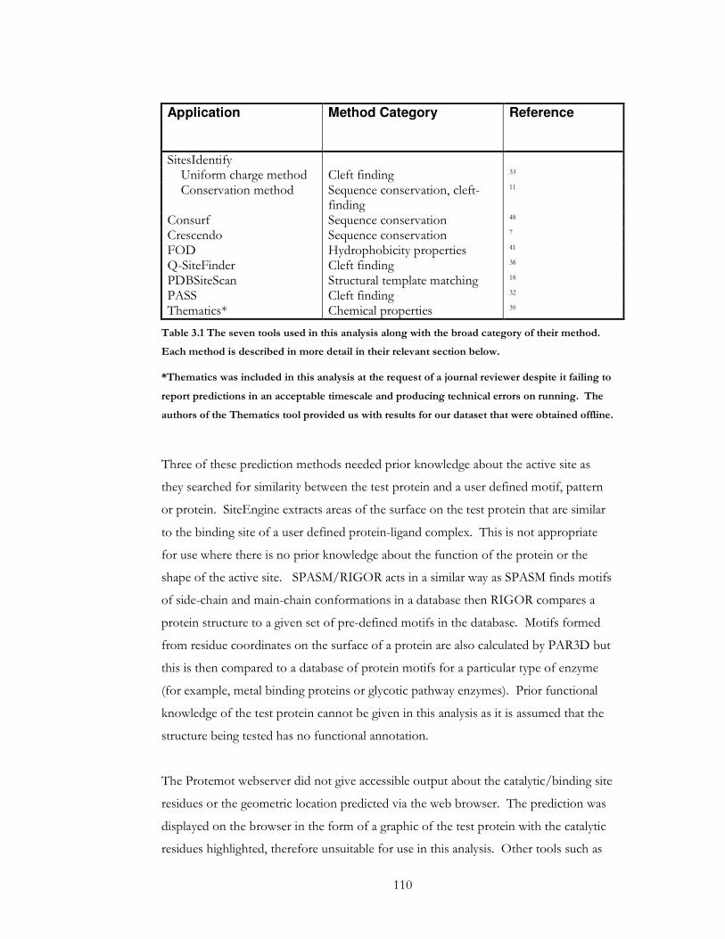
110

Application

Method Category Reference

SitesIdentify Uniform charge method Cleft finding 33 Conservation method Sequence conservation, cleft-

finding 11

Consurf Sequence conservation 48 Crescendo Sequence conservation 7 FOD Hydrophobicity properties 41 Q-SiteFinder Cleft finding 38 PDBSiteScan Structural template matching 18 PASS Cleft finding 32 Thematics* Chemical properties 39

Table 3.1 The seven tools used in this analysis along with the broad category of their method.

Each method is described in more detail in their relevant section below.

*Thematics was included in this analysis at the request of a journal reviewer despite it failing to

report predictions in an acceptable timescale and producing technical errors on running. The

authors of the Thematics tool provided us with results for our dataset that were obtained offline.

Three of these prediction methods needed prior knowledge about the active site as

they searched for similarity between the test protein and a user defined motif, pattern

or protein. SiteEngine extracts areas of the surface on the test protein that are similar

to the binding site of a user defined protein-ligand complex. This is not appropriate

for use where there is no prior knowledge about the function of the protein or the

shape of the active site. SPASM/RIGOR acts in a similar way as SPASM finds motifs

of side-chain and main-chain conformations in a database then RIGOR compares a

protein structure to a given set of pre-defined motifs in the database. Motifs formed

from residue coordinates on the surface of a protein are also calculated by PAR3D but

this is then compared to a database of protein motifs for a particular type of enzyme

(for example, metal binding proteins or glycotic pathway enzymes). Prior functional

knowledge of the test protein cannot be given in this analysis as it is assumed that the

structure being tested has no functional annotation.

The Protemot webserver did not give accessible output about the catalytic/binding site

residues or the geometric location predicted via the web browser. The prediction was

displayed on the browser in the form of a graphic of the test protein with the catalytic

residues highlighted, therefore unsuitable for use in this analysis. Other tools such as

111

Crescendo and FOD did not explicitly give residue identities or geometric locations but

gave per-residue scores related to their measures. Predictions were then made by

taking a set of top-scoring residues from the output (see the description of each

method below for the criteria).

Due to the large number of proteins used in the test set (237 enzymes), the time taken

to compute predictions is important to this analysis. Five of the methods took

inappropriate amounts of time to compute results, these usually included methods that

had some conservation-related aspect to them. FrPred uses conservation information

and was problematic to run as it could only handle proteins with less than 500 residues.

Even proteins with a length less than this, however, took a large amount of time to

run. PinUP also uses conservation scoring in its method and thus took unsuitable

lengths of time to compute. SuMo compares the test proteins to all ligand binding sites

in the PDB database. It gives the option of using only part of the test protein and/or a

subset of PDB files to search against, however, using the whole protein and

exhaustively searching against the whole PDB database takes a prolonged amount of

time.

PDBSiteScan, whilst used in this analysis, transfers annotation from similar proteins in

the PDB. As this test set contains proteins with known active site information it is

likely to retrieve information from the test protein in the PDB database. In this

analysis, a prediction from PDBSiteScan has been removed if the information was

obtained from the same structure as the test structure. Another method, CSS, scans

the CSA in order to compare the test protein to proteins with annotation in the CSA.

It was deemed unsuitable for this analysis since the test set is derived from the CSA

and so the top active site prediction for each protein in the test set was annotation

transferred from itself.

112

The remaining six prediction methods (CrPred, FSPS, MFS, PINTS, PvSOAR and

SARIG) could not be included in the analysis for technical reasons. CrPred’s

predictions were pre-computed for specific datasets of structurally related proteins.

This was deemed unsuitable for the methods later use in a function prediction method.

The web server was inaccessible for PvSOAR, whilst the PINTS web server gave

errors and the web page containing SARIGs output also gave errors. The web server

for MFS was unreliable and often gave error messages, whilst the command-line

download option did not give a single prediction program but a list of standalone

feature calculation programs with no instruction as to order of running or

interpretation of output.

113

Name Reference publication Reason for non-inclusion in analysis

CrPred Zhang et al., (2008) Technical reasons. CSS Torrence et al. (2005) Scans test set. FrPred Fischer et al. (2007) Processing time.

(could only process <500 residues)

Functional Site Prediction Server (FSPS)

Cheng et al. (2005) Technical reasons.

MFS Wang et al. (2008) Technical reasons. Par3D Goyal et al. (2007) Prior knowledge needed PINTS Stark and Russell (2003) Technical reasons. PinUP Liang et al. (2006) Processing time. Protemot Chang et al. (2006) Cannot process results PvSOAR Binkowski et al. (2004) Technical reasons. SARIG Amitai et al. (2004) Technical reasons. SiteEngine Shulman-Peleg et al. (2005) Prior knowledge needed SPASM/RIGOR Kleywegt (2005) Prior knowledge needed SuMo Jambon et al. (2005) Processing time.

Table 3.2: Functional site prediction tools not included in the comparison analysis. Reasons

for non-inclusion in the analysis are further explained below:

Technical reasons. Web-servers that produced errors on attempting to submit a protein or

accessing results pages were not included.

Prior knowledge needed. These prediction methods needed prior knowledge about the active

site as they search for similarity between the test protein and a user defined motif, pattern or

protein.

Cannot process results. The results are not given in a form that can be automatically processed

(in this case the prediction was displayed as a graphic of the test protein with the catalytic

residues highlighted).

Processing time. Due to the large number of proteins used in the test set (237), the time taken

to compute predictions is important to this analysis. A tool was excluded if results were not

returned within 10 minutes for an example test protein of 330 residues (PDBID: 12as).

Scans test set. CSS scans the CSA in order to compare the test protein to proteins with

annotation in the CSA. It was deemed unsuitable for this analysis since the test set is derived

from the CSA.

114

3.2.2 Creation of Test Sets

Two datasets are used in this analysis; an enzyme set and a non-enzyme set. As

mentioned previously, enzymes are usually used to test functional site predictors due to

their functional sites being easily defined by the location of their catalytic residues. The

primary dataset that these methods are tested on is the enzyme dataset, however to

assess each method’s applicability to other types of proteins a non-enzyme dataset was

also gathered.

The enzyme dataset was gathered from the 880 literature annotated entries in version

2.2.1 of the Catalytic Sites Atlas (CSA) database14. In order to reduce bias towards

methods that are particularly good at classifying a particular enzyme (and its related

homologues) it was important to remove redundancy from this dataset. The set of 880

proteins were culled for redundancy on the basis that no two enzymes shared an active

site-containing domain from the same SCOP superfamily with any other protein of a

lesser structural quality. This procedure is described in more detail in Chapter 2,

however in this analysis the enzymes were not split into EC classes.

The resultant dataset contained 237 enzymes, each having one or more annotated

active sites (see Table 3.3). This gave a total of 747 catalytic residues with an average

of 3.2 catalytic residues per site per protein.

115

1ssx 1h2r 1dxe 1gpr 2plc 1b65 1eb6 1gcu 1c3c 1f7l 1wgi 1al6 1p1x 1g6t 1bp2 1c3j 1r16 1abr 1qj4 1dw9 2jcw 1bg0 1pa9 12as 1qv0 2xis 2acy 1sox 1oas 1rbl 1itx 1ru4 1qrg 1qcn 1nsp 1qd6 2nlr 1d3g 1qaz 1gog 1nid 1pya 1nww 1uaq 1e1a 1fua 1m9c 1pfk 1qtn 1s95 1cg6 1d6o 1gpj 1nir 1o9i 1r6w 1uro 1d0s 1eh6 1n20 1e7l 1qq5 1tys 1bs4 1e2a 1nn4 2tps 1moq 1tml 1b93 1bou 1mvn 2pth 1lam 1j79 1apy 1a05 1mqw 1vlb 1jnr 1foa 1a4i 2cpo 1ef0 1qje 1dl2 1chd 1a2t 1yve 1cd5 1fy2 1cs1 1r51 1mrq 1nml 1r4f 1dbf 1aop 1pgs 1l1d 1lci 1q3q 1nlu 1v0y 1p4n 1kp2 1f75 1ndo 1rhs 1qgx 1oe8 1jhf 1bol 1f8x 1hdh 1eug 1lbu 1jdw 1aj0 1dhf 2eng 7odc 1jh6 1i6p 1otg 1cev 1c0k 1uqr 1j53 1chm 1k4t 3nos 135l 1qhf 1j09 1akd 1fro 3mdd 7atj 1qd1 1g72 1oj4 1f2v 2toh 1pyl 1p3d 1dup 1oac 1dmu 1d8h 1nln 1o04 1d4a 1hxq 1c2t 1a79 1nf9 1gqg 1cgk 1vid 1bwp 1vas 1dj0 1d1q 2sqc 1pii 3eca 1jms 1oyg 1ako 1tph 1js4 2ypn 1dve 1mla 2bbk 1pud 1do6 1uam 1dqa 1m6k 2apr 1m21 1aug 1lij 1c9u 1e19 2ahj 1l1l 1a95 1lba 1b5t 1qh5 1j7g 1g24 1nhx 1k82 1qpr 1dci 1i19 1daa 1hrk 1h3i 1dco 1p5d 1dae 1uf7 1g79 1ez1 1r76 1ah7 1rhc 1ro7 1fgh 1dqs 1bt1 1snn 3cla 1mka 1ecm 1dnp 1jm6 1l6p 1mud 1k30 1ecl 1dio 1hka 1kaz 1jfl 1d8c 1ca3 1hfe 1fnb 1ir3 1d2t 1brw Table 3.3 The PDB codes for the 237 structures in the enzyme dataset

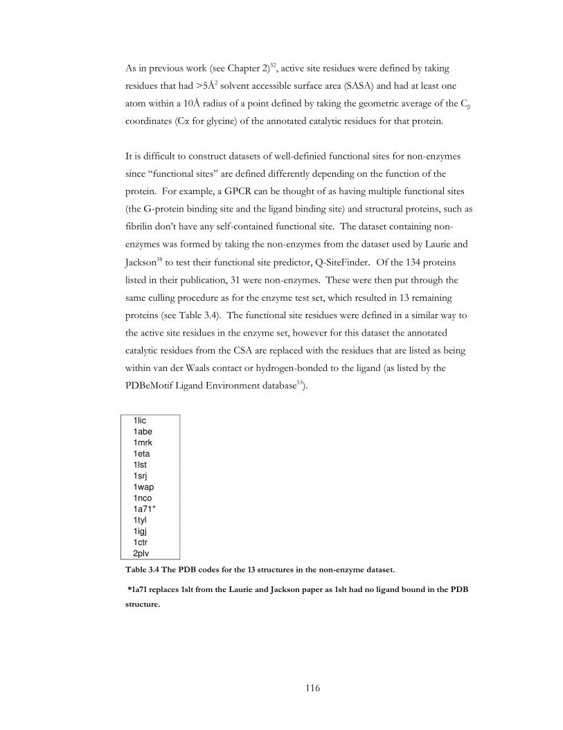
116

As in previous work (see Chapter 2)52, active site residues were defined by taking

residues that had >5Å2 solvent accessible surface area (SASA) and had at least one

atom within a 10Å radius of a point defined by taking the geometric average of the Cβ

coordinates (Cα for glycine) of the annotated catalytic residues for that protein.

It is difficult to construct datasets of well-definied functional sites for non-enzymes

since “functional sites” are defined differently depending on the function of the

protein. For example, a GPCR can be thought of as having multiple functional sites

(the G-protein binding site and the ligand binding site) and structural proteins, such as

fibrilin don’t have any self-contained functional site. The dataset containing non-

enzymes was formed by taking the non-enzymes from the dataset used by Laurie and

Jackson38 to test their functional site predictor, Q-SiteFinder. Of the 134 proteins

listed in their publication, 31 were non-enzymes. These were then put through the

same culling procedure as for the enzyme test set, which resulted in 13 remaining

proteins (see Table 3.4). The functional site residues were defined in a similar way to

the active site residues in the enzyme set, however for this dataset the annotated

catalytic residues from the CSA are replaced with the residues that are listed as being

within van der Waals contact or hydrogen-bonded to the ligand (as listed by the

PDBeMotif Ligand Environment database53).

1lic

1abe

1mrk

1eta

1lst

1srj

1wap

1nco

1a71*

1tyl

1igj

1ctr

2plv

Table 3.4 The PDB codes for the 13 structures in the non-enzyme dataset.

*1a71 replaces 1slt from the Laurie and Jackson paper as 1slt had no ligand bound in the PDB

structure.

117

3.2.3 Obtaining and Unifying Functional Site Predictions

The predictions for each method were obtained by automatically running the dataset

through each webserver and capturing the output via a perl-CGI script for

QSiteFinder, Consurf, PDBSiteScan and FOD. Thematics and Crescendo were unable

to be run automatically online for large datasets and therefore the results were provided

by their respective groups from offline runs. Due to availability of source code, results

from SitesIdentify and PASS were obtained from running the code locally. The

asymmetric unit structure file was supplied to each method on the basis that a newly

solved structure of a protein of unknown function would be unlikely to have any clear

indication of its true in vivo quaternary structure. Some methods can only deal with one

chain and where this is the case only the first chain in the file has been passed to the

method.

SitesIdentify and PASS give predictions by specifying PDB geometry coordinates

relating to the centre of the active site, which is used directly as the centroid for further

defining active site residues. For methods that give output in the form of a number of

predicted residues (whether that be catalytic only in the case of enzymes or a set of site

environment residues) the centroid is calculated by averaging the Cβ atom coordinates

(Cα for glycine). The standardised predicted residues used to assess the prediction

accuracy of each method are defined as those that have at least one atom within a 10Å

radius of this centroid and have a SASA of 5Å2 or more. This provides standardised

output that can be fairly compared between the different methods.

Prediction accuracy can be measured in a number of different ways; the most simple is

measuring the linear distance between the real site centroid and the predicted centroid.

This measure may, however, be misleading due to the geometry of the functional site.

The predicted and real centroid may be some distance apart whilst the environment

around each centroid may contain most of the same residues, therefore identifying the

same site.

It is possibly more important to consider how many of the biologically active residues

(i.e. catalytic in the case of enzymes and ligand-binding in non-enzymes) are recalled as

118

predicted site residues by each method. It is important to note however, that in the

enzyme dataset the active site residues defined using the CSA generated centroid do

not recall 100% of the CSA annotated catalytic residues (see Figure 3.2 and Table 3.5).

It is therefore unfair to evaluate a method by its absolute CSA/ligand-binding residue

recall rate (termed the absolute recall rate). It is more realistic to compare its

CSA/ligand-binding residue recall rate to the recall rate achieved by the real centroid

(termed the relative recall rate).

In the previous analysis of structural and sequence features of active sites (Chapter 2),

many features were found that differed significantly between enzyme functions. These

features were calculated on the active site residues defined by the CSA generated

centroid. The best performing method from this analysis will go on to be used to

predict active site residue sets of unknown proteins in order to calculate values for

features in the same way as in the previous study. The number of residues that are

shared between the real active site residue set and the predicted active site residue set is

therefore of interest. It should not be taken as a definite measure of a method’s

accuracy as it has limited relevance outside of the use of this study.

It is also important to consider which site on a protein is being predicted. There may

be more than one genuine active site on a given structure, particularly where there are

symmetrical chains. The CSA annotation deals with this by providing a number of site

entries per protein. When a site is predicted by a method, it is assessed to see which

real site listed in the CSA the predicted site is closest to. It would be unfair to compare

a prediction simply to the first site in the CSA if it happened to be on an opposite

symmetrical chain as this would produce a falsely erroneous result (see Figure 3.1).

Similarly in the non-enzyme dataset, where there is more than one identical site there

will be multiple bound ligands in the PDB file. Ligand-binding residues for these

multiple ligands are split into their respective sites.

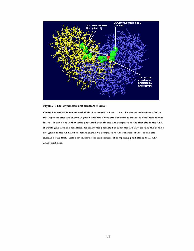
119

Figure 3.1 The asymmetric unit structure of 1daa.

Chain A is shown in yellow and chain B is shown in blue. The CSA annotated residues for its

two separate sites are shown in green with the active site centroid coordinates predicted shown

in red. It can be seen that if the predicted coordinates are compared to the first site in the CSA,

it would give a poor prediction. In reality the predicted coordinates are very close to the second

site given in the CSA and therefore should be compared to the centroid of the second site

instead of the first. This demonstrates the importance of comparing predictions to all CSA

annotated sites.

120

3.3 Methods: SitesIdentify Webserver

3.3.1 Functional Site Prediction Methods

SitesIdentify can predict functional site location by two separate approaches, which

have been published previously11; 33 The first method essentially identifies buried clefts

on the surface of the protein via electrostatics calculations33. In a previous publication

by Bate and Warwicker, a number of electrostatic properties were used to attempt to

identify active sites in enzymes. A 2Å grid was placed over the protein and the

electrostatic potential from the atoms contained within the neighboring grid volumes is

calculated for each second nearest grid point to the protein’s surface. The electrostatic

potential was calculated firstly by assigning charges to all ionisable residues based on

model pKas at pH 5.5, pH 7 and irrespective of pH, and secondly by applying a

uniform charge density to all Cα atoms from all non-hydrogen residues. The electric

potential is calculated at each grid point using finite difference Poisson-Boltzmann

(FDPB) calculations and the grid point that had the greatest peak potential was

predicted to be the active site centre coordinate.

The peak-potential calculations from applying estimated charges from pKa didn’t,

however, perform as well as the simpler uniform charge density method. The peak

potential from the uniform charge method therefore essentially identifies the most

buried cleft on the protein surface. Here, this method is termed SitesIdentify(GM),

where GM stands for geometric.

The second method of SitesIdentify presented here is based on the uniform charge

method but the charges are weighted with normalised conservation scores that reflect

the amino acid/sterochemical diversity and the gap occurrence of that residue (see

Equation 3.1). Close homologues are found by running the sequence through PSI-

BLAST with an E value cut-off of 1e-20 and then a profile is created from which the

conservation score is calculated. The peak potential on the grid is then calculated by

FDPB calculation by using the conservation-weighted charges on each residue. This

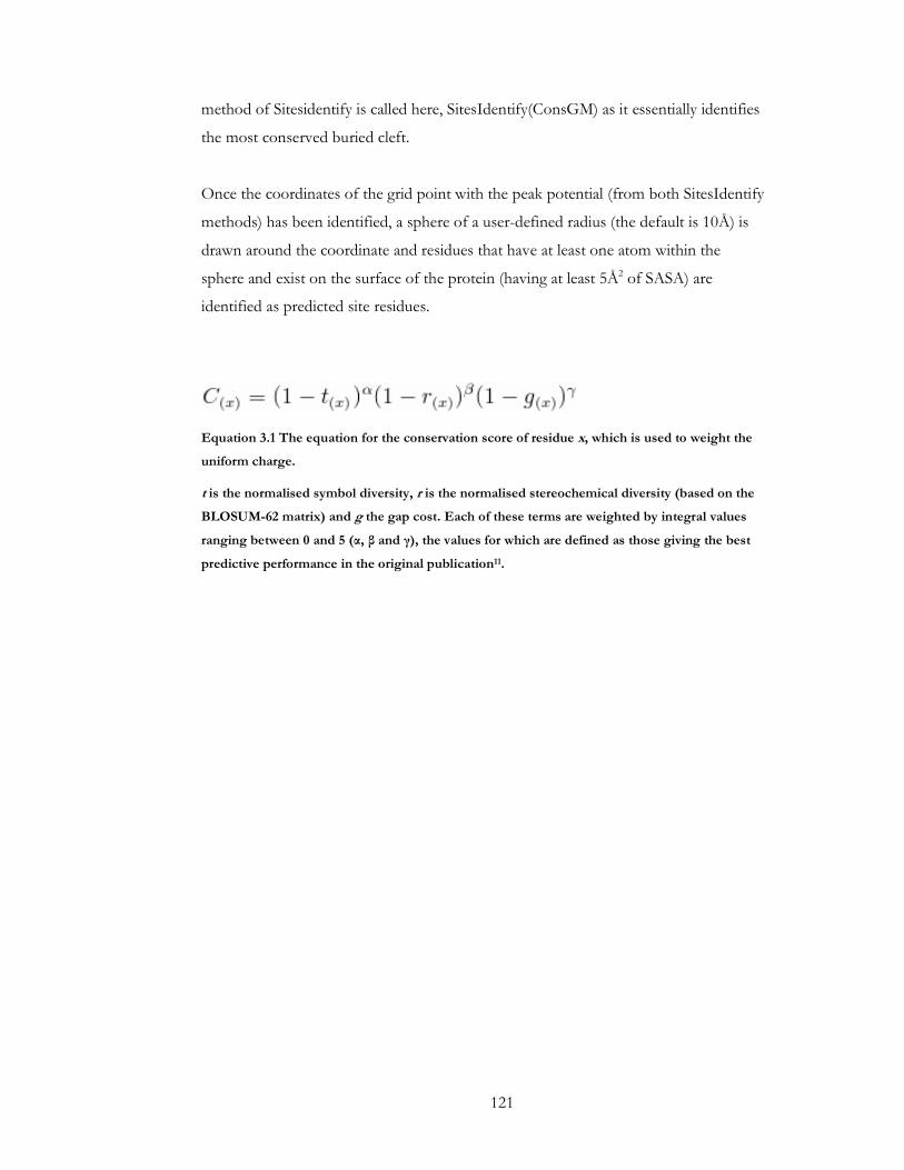
121

method of Sitesidentify is called here, SitesIdentify(ConsGM) as it essentially identifies

the most conserved buried cleft.

Once the coordinates of the grid point with the peak potential (from both SitesIdentify

methods) has been identified, a sphere of a user-defined radius (the default is 10Å) is

drawn around the coordinate and residues that have at least one atom within the

sphere and exist on the surface of the protein (having at least 5Å2 of SASA) are

identified as predicted site residues.

Equation 3.1 The equation for the conservation score of residue x, which is used to weight the

uniform charge.

t is the normalised symbol diversity, r is the normalised stereochemical diversity (based on the

BLOSUM-62 matrix) and g the gap cost. Each of these terms are weighted by integral values

ranging between 0 and 5 (α, β and γ), the values for which are defined as those giving the best

predictive performance in the original publication11.

122

3.3.2 SitesIdentify Workflow

Upon submission of a job, SitesIdentify starts a number of programs depending on

which method the user requested. If the conservation approach is selected, the in-

house Conserved Residue Colouring program(CRC) is run first, which identifies

homologues by running the sequence contained in the SEQRES records in the PDB

file through PSI-BLAST 54. PSI-BLAST is run for one iteration (in default settings) on

the non-redundant database with an E-value cut-off for inclusion of sequences of 1e-

20. A profile file containing the conservation scores for each residue is produced.

SitesIdentify uses the conservation scores as charge weightings on a single atom for

each amino acid (Cβ or Cα for glycine), and calculates the location of the peak potential

as described above 11.

If no homologue can be identified for a protein using CRC then the method

automatically switches to only charge-based calculations. If the conservation method is

not selected then the CRC program is omitted and the location of the peak potential is

calculated using the uniform charge-weighting method 33. A sphere of user-supplied

radius is drawn around the predicted centroid coordinates and residues are selected that

have at least one atom within that sphere and also exhibit more than 5Å2 of solvent-

accessible surface area (SASA) as calculated using the Lee and Richards method 55. This

list of residues represents the predicted functional site, which is given on the results

page as a text list and also highlighted on the PDB structure using Jmol 56 .

3.3.3 SitesIdentify Usage

SitesIdentify is available for use via a web browser and is freely accessible without

license or an account registration. The main web page allows a user to enter either a

pre-existing PDB structure ID (and whether to use the biological unit or the

asymmetric unit) or upload a structure file, the radius around the predicted site to use,

the method to use and an email address so that a user can be notified and emailed the

results link upon job completion.

123

If a user has submitted their own structure file then this is validated to ensure that

contains an acceptable PDB-format structure, the rules for which are given in the user

guide available from the website. The file must be less than 2MB in size and contain

only text. It also must contain at least SEQRES and ATOM records and be spaced

exactly as the standard PDB format. If the user-supplied information is invalid (non-

existent PDB ID or invalid email address) then the job is not initialised and the user

informed of the incorrect information via the browser. Upon successful completion of

a job the web-server directs the user to the results page and also sends an email to the

user at the address specified with a link to the results page.

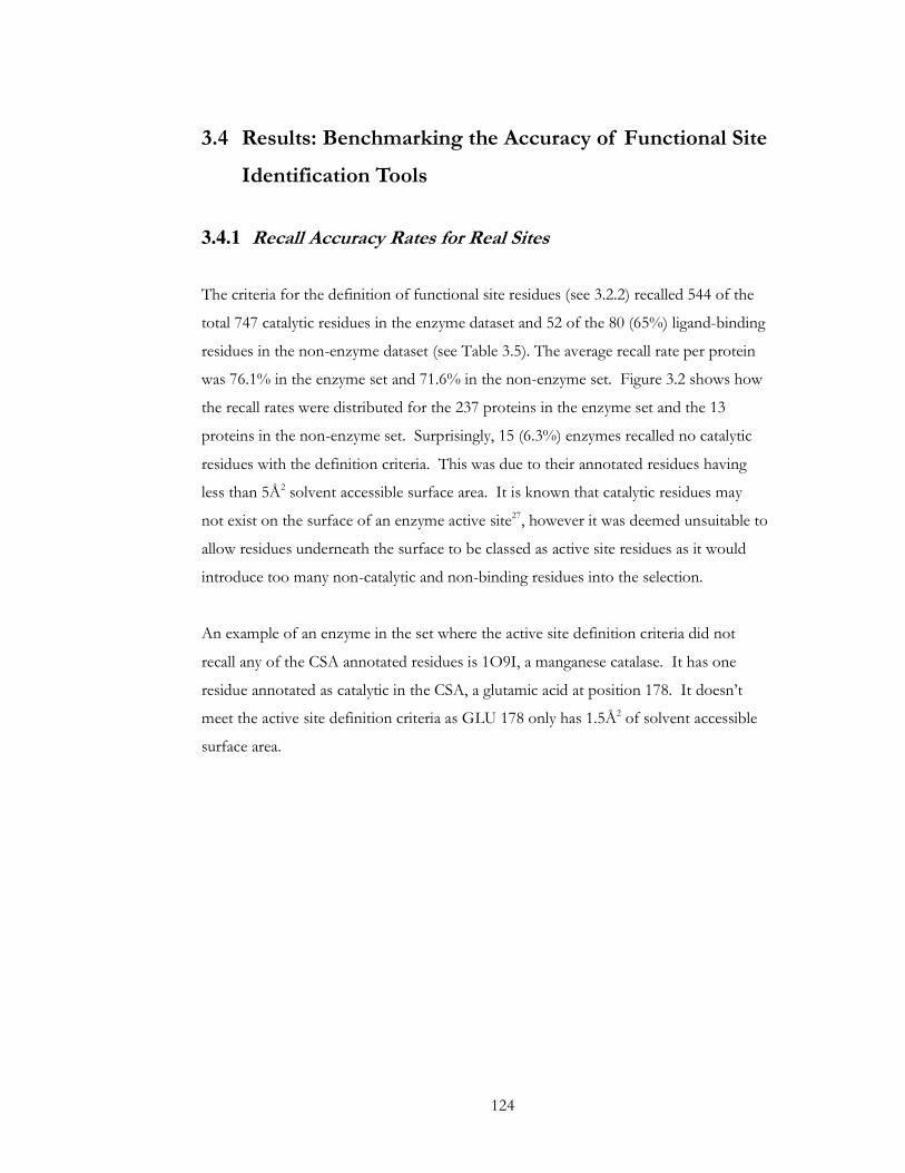
124

3.4 Results: Benchmarking the Accuracy of Functional Site

Identification Tools

3.4.1 Recall Accuracy Rates for Real Sites

The criteria for the definition of functional site residues (see 3.2.2) recalled 544 of the

total 747 catalytic residues in the enzyme dataset and 52 of the 80 (65%) ligand-binding

residues in the non-enzyme dataset (see Table 3.5). The average recall rate per protein

was 76.1% in the enzyme set and 71.6% in the non-enzyme set. Figure 3.2 shows how

the recall rates were distributed for the 237 proteins in the enzyme set and the 13

proteins in the non-enzyme set. Surprisingly, 15 (6.3%) enzymes recalled no catalytic

residues with the definition criteria. This was due to their annotated residues having

less than 5Å2 solvent accessible surface area. It is known that catalytic residues may

not exist on the surface of an enzyme active site27, however it was deemed unsuitable to

allow residues underneath the surface to be classed as active site residues as it would

introduce too many non-catalytic and non-binding residues into the selection.

An example of an enzyme in the set where the active site definition criteria did not

recall any of the CSA annotated residues is 1O9I, a manganese catalase. It has one

residue annotated as catalytic in the CSA, a glutamic acid at position 178. It doesn’t

meet the active site definition criteria as GLU 178 only has 1.5Å2 of solvent accessible

surface area.

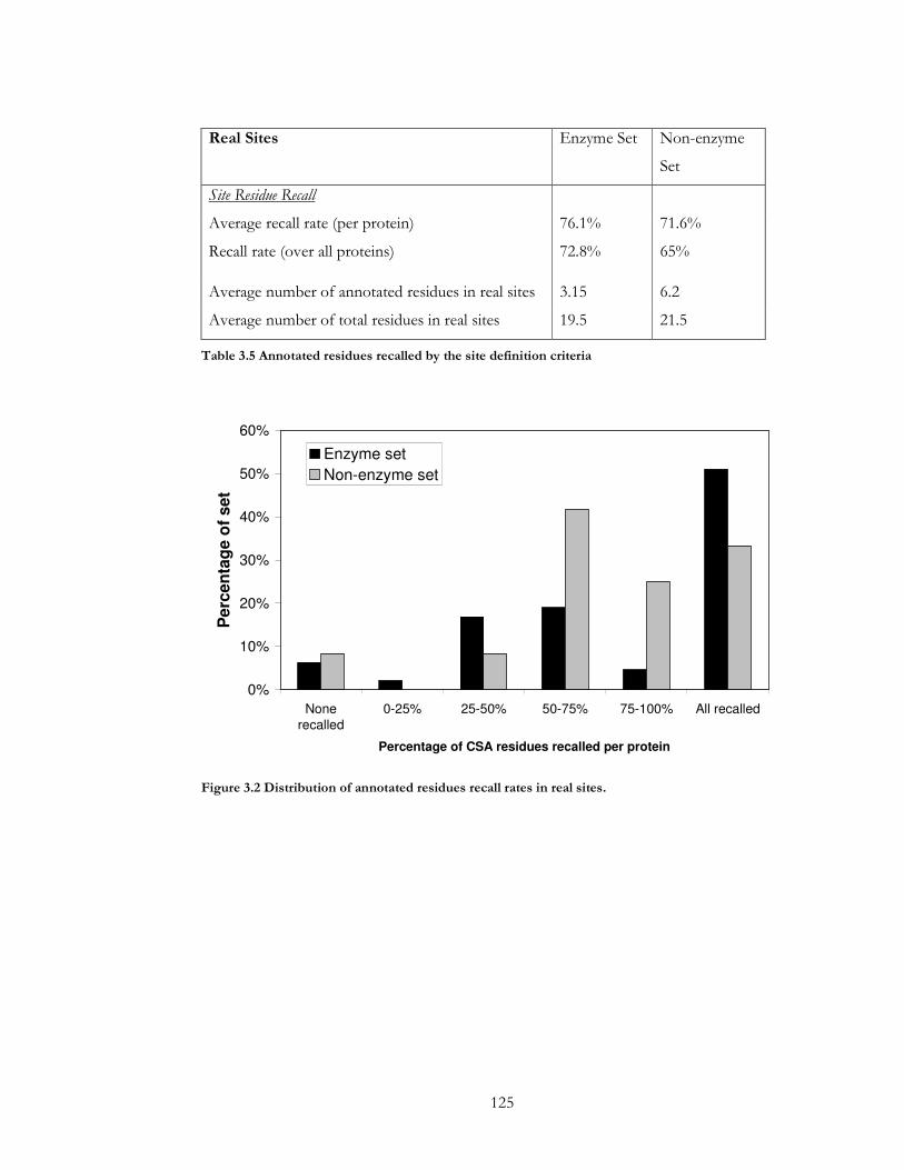
125

Real Sites Enzyme Set Non-enzyme

Set

Site Residue Recall

Average recall rate (per protein) 76.1% 71.6%

Recall rate (over all proteins) 72.8% 65%

Average number of annotated residues in real sites 3.15 6.2

Average number of total residues in real sites 19.5 21.5

Table 3.5 Annotated residues recalled by the site definition criteria

0%

10%

20%

30%

40%

50%

60%

None

recalled

0-25% 25-50% 50-75% 75-100% All recalled

Percentage of CSA residues recalled per protein

Per

cen

tag

e o

f se

t

Enzyme set

Non-enzyme set

Figure 3.2 Distribution of annotated residues recall rates in real sites.

126

3.4.2 Crescendo

Method Description

Crescendo seeks to identify active sites by identifying clusters of residues that have

higher than usual evolutionary constraint. Residues under evolutionary constraint were

identified by three measures; 1) whether there was a higher degree of evolutionary

conservation than expected at a position, 2) whether environment specific substitution

tables made weak predictions of the amino acid substitution patterns, and 3) residues

that have spatially conserved positions when structures of proteins within the same

family are superimposed. The method is able to distinguish between residues that are

conserved for structural or functional regions.

In the reference paper7, the scores calculated by these measures are overlaid onto the

protein structure and clusters of high scoring residues are identified and predicted as

functional site locations. The method provided in the webserver however, omits this

stage of the process and returns restraint scores on a per residue basis for the whole

protein. A user can then load this PDB format file into a molecular graphics program

to visually scan for clusters of highly conserved residues. Since this analysis calls for

the automatic identification of functional sites without visual inspection, site residues

are identified by taking a sample of the top-scoring residues. The average number of

functional residues per protein over the three test sets that the authors used was 6.8.

In our testing dataset there is an average of 3.2 literature annotated catalytic residues

per enzyme, which is similar to the average number of 3.5 annotated catalytic residues

per protein quoted in the original CSA analysis27. As a compromise between these

figures, the top 5 scoring residues given in the crescendo output were taken as the

predicted functional residues.

127

Prediction Accuracy

Predictions were obtained successfully for each of the 237 proteins in the enzyme set

and each of the 13 proteins in the non-enzyme set. Crescendo only evaluates one

chain so the first chain identifier in the PDB was used. Despite this limitation

Crescendo performed well (see Table 3.6), achieving a relative recall rate of 63.8% for

the enzyme set and 65.8% for the non-enzyme set. The distribution of distances

between predicted centroids and real centroids is shown in Figure 3.4.

In the enzyme set Crescendo performed better than the CSA defined active site for

two structures, 1e2a and 1f8x. The CSA defined centroid recalled 2 out of the 4

annotated residues for 1e2a whilst Crescendo recalled 3 out of 4. Crescendo recalled

all of the 4 annotated residues for 1f8x, whilst the CSA generated centroid only recalled

3. Crescendo recalled more annotated residues than the real centroid for 6 of the 13

proteins in the non-enzyme set.

Crescendo Enzyme Set Non-enzyme

Set

Site Residue Recall

Absolute recall rate 46.9% 44.2%

Relative recall rate 63.8% 65.8%

Distance between real and predicted centroids

Average distance (Ǻ) 10.3 11.8

Minimum distance (Ǻ) 1.0 2.9

Maximum distance (Ǻ) 28.4 33.8

Site residues shared between real and predicted sites

Average number of residues in real sites 19.6 21.5

Average number of residues in predicted sites 18.3 21.2

Average number of site residues shared 7.1 9.1

Average percentage of site residue shared per protein 35.7% 44.3%

Table 3.6 The functional site prediction accuracy results for Crescendo.

128

A

0%

10%

20%

30%

40%

50%

60%

None

recalled

0-25% 25-50% 50-75% 75-100% All recalled


Per

cen

tag

e o

f se

t

Real sites

Predictedsites

B

0%

5%

10%

15%

20%

25%

30%

35%

40%

45%

None

recalled

0-25% 25-50% 50-75% 75-100% All recalled

Percentage of annotated residues recalled per protein

Per

cen

tag

e o

f se

t

Real sites

Predictedsites

Figure 3.3 The distribution of absolute recall rates per protein for Crescendo in A) the enzyme

set and B)the non-enzyme set.

129

0%

10%

20%

30%

40%

50%

60%

70%

80%

90%

100%

0 5 10 15 20 25 30 35 40 45 50

Distance between predicted and real centroid (rounded to nearest Ångstrom)

Cu

mu

lati

ve p

erce

nta

ge

of

set

Enzymes

Non-enzymes

Figure 3.4 The cumulative percentage of distances between Crescendo-predicted and real

centroids within the two sets.

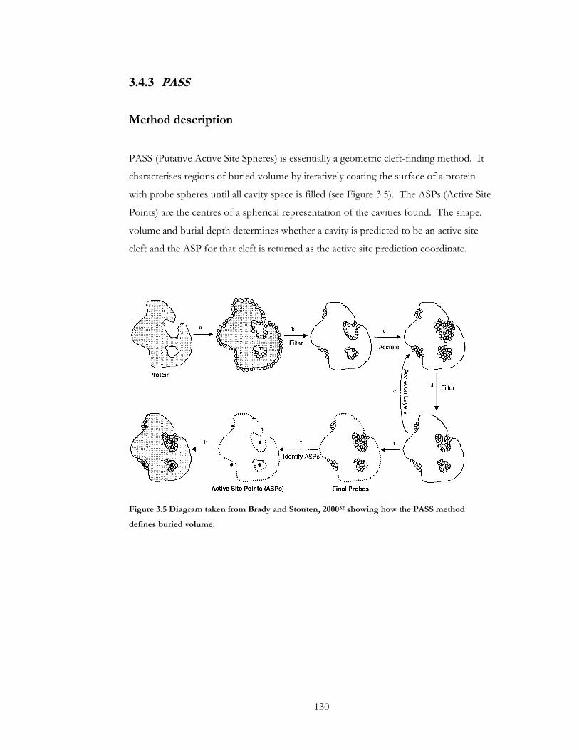
130

3.4.3 PASS

Method description

PASS (Putative Active Site Spheres) is essentially a geometric cleft-finding method. It

characterises regions of buried volume by iteratively coating the surface of a protein

with probe spheres until all cavity space is filled (see Figure 3.5). The ASPs (Active Site

Points) are the centres of a spherical representation of the cavities found. The shape,

volume and burial depth determines whether a cavity is predicted to be an active site

cleft and the ASP for that cleft is returned as the active site prediction coordinate.

Figure 3.5 Diagram taken from Brady and Stouten, 200032 showing how the PASS method

defines buried volume.

131

Prediction accuracy

PASS did not run successfully for 9 proteins in the enzyme dataset and for one protein

in the non-enzyme set. For two further structures in the enzyme set, 1bs4 and 1qdl,

and one in the non-enzyme set (1eta) the centroid coordinates given were not within

the coordinate limits of the protein structure and thus no residues could be found

within the 10Ǻ of the centroid predicted. PASS achieved an average relative recall rate

of 49.3% for enzymes and 44.1% for non-enzymes.

Putative Active Sites with Spheres (PASS) Enzyme Set Non-enzyme

Set

Site Residue Recall












Table 3.7 The functional site prediction accuracy results for PASS.

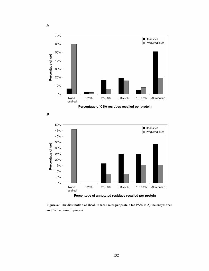
132

A

0%

10%

20%

30%

40%

50%

60%

70%

Nonerecalled

0-25% 25-50% 50-75% 75-100% All recalled


Per

cen

tag

e o

f se

t

Real sites

Predicted sites

B

0%

5%

10%

15%

20%

25%

30%

35%

40%

45%

50%

Nonerecalled

0-25% 25-50% 50-75% 75-100% All recalled


Per

cen

tag

e o

f se

t

Real sites

Predicted sites

Figure 3.6 The distribution of absolute recall rates per protein for PASS in A) the enzyme set

and B) the non-enzyme set.

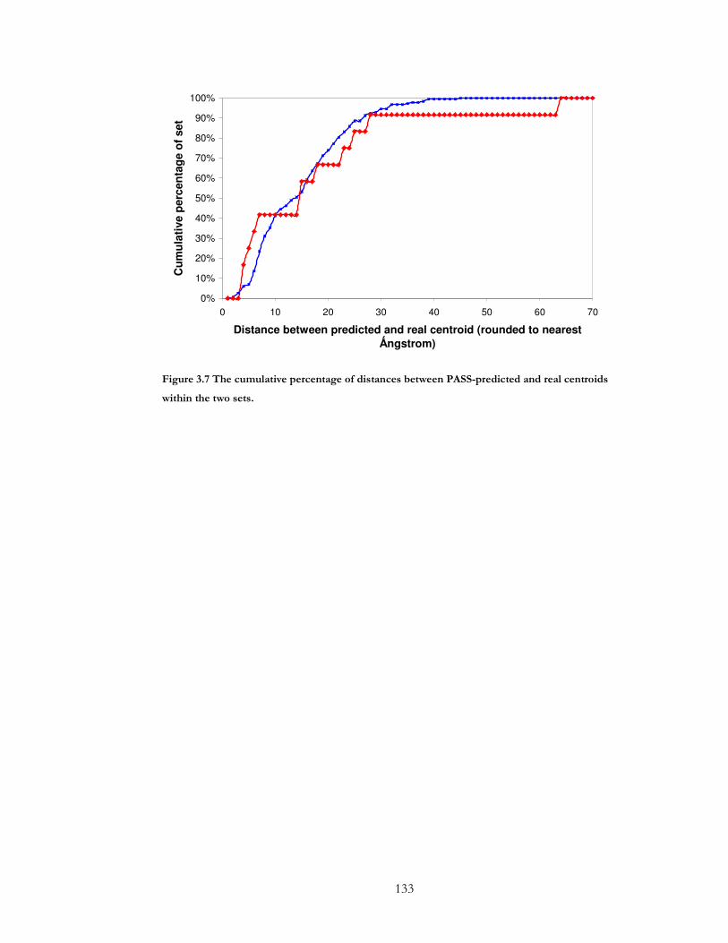
133

0%

10%

20%

30%

40%

50%

60%

70%

80%

90%

100%

0 10 20 30 40 50 60 70

Distance between predicted and real centroid (rounded to nearest Ǻngstrom)

Cu

mu

lati

ve p

erce

nta

ge

of

set

Figure 3.7 The cumulative percentage of distances between PASS-predicted and real centroids

within the two sets.

134

3.4.4 Fuzzy Oil Drop

Method description

It has long been observed that residues in the solvent-inaccessible core of a protein are

more likely to be more hydrophobic than the residues existing on, or close to, the

surface of a protein57. Residues involved in binding have been shown to frequently

exhibit levels of hydrophobicity that are unusual for their position within the protein

structure58. This prediction method predicts residues as forming a functional site

where there is a large difference between the expected hydrophobicity of a residue at

that position and the observed hydrophobicity value.

The hydrophobicity force field calculated in this method is based on the assumption

that the theoretical hydrophobicity in proteins follows a 3D Gaussian distribution. The

expected hydrophobicity of a residue is determined by a residues relative position to

the theoretically most hydrophobic point in the protein. The observed hydrophobicity

value is calculated by assessing the hydrophobicity characteristics of the sidechains

within the protein model and the residues position in relation to those side chains.

They have shown that this model does not produce significantly different results to

more commonly used scales such as Eisenberg59 and Kyte and Doolittle60 scales.

The hydrophobic deficiency score for each residue is the difference between the

expected hydrophobicity and the observed hydrophobicity. The highest scoring

residues are then predicted to be involved in functional sites. The residues were then

ranked by descending score and the minimum score of top 5% residues were then

predicted as functional site residues as the reference paper instructs.

135

Prediction accuracy

As with Crescendo, the FOD method can only calculate predictions of a single

polypeptide chain and so the first chain in the PDB file was used. Predictions were

obtained successfully for all 237 proteins in the enzyme set, giving relative recall rate of

56.1% and for 12 of the 13 non-enzymes giving a relative recall rate of 33.3% (Table

3.8). There were, however, some issues in the output that meant a slightly altered

analysis was required.

One issue was that the residue numbering in their output was different to the

numbering of residues in the PDB. The output of this method includes a modified

PDB file that uses their own numbering scheme and so centroids were calculated from

this PDB file instead of the standard PDB file. The PDB file supplied in the output

occasionally misses atom coordinates for some of their predicted active site residues.

Where the Cβ atom coordinates for a predicted residue were unavailable in the output

PDB file, the coordinates for the next available atom in that residue were used in order

to calculate the centroid.

The second issue was that the hydrophobic deficiency score applied to each residue

was truncated to 2 decimal places in the output in order for it to be accommodated

into the temperature factor column of the PDB format file. This produced degeneracy

in the scoring system since multiple residues could be assigned the same score.

Multiple residues having the same score created a problem when attempting to cut off

the top 5% scoring residues to predict as active site residues. The boundary residue for

the top 5% often lay within a group of residues with the same score and therefore

discriminating which of these residues to consider a prediction is somewhat arbitrary.

The output for the method also gives the raw (un-normalised) hydrophobic deficiency

score for each residue. In order to avoid the above problem, the residues with the top

5% of raw hydrophobic deficiency values (rather than normalised, as reported in their

publication) were predicted as active site residues.

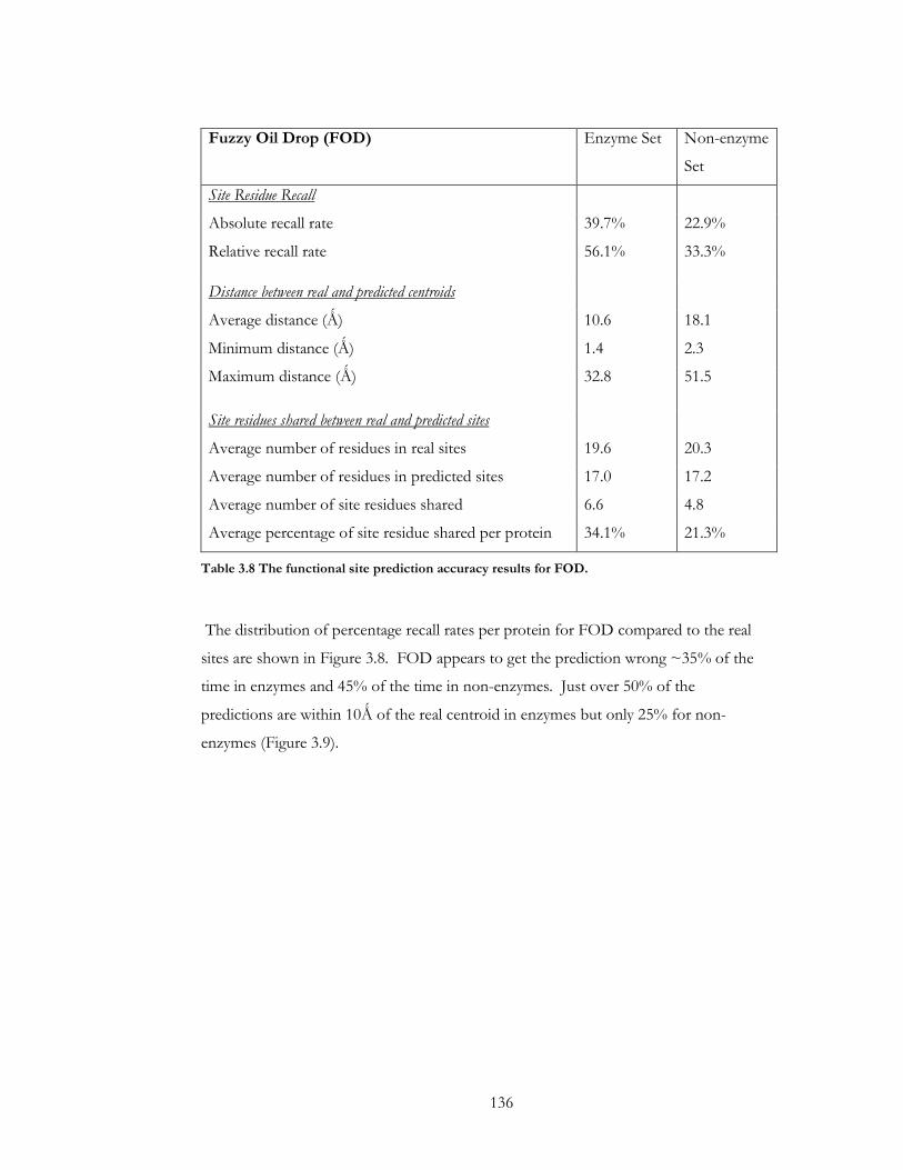
136

Fuzzy Oil Drop (FOD) Enzyme Set Non-enzyme

Set

Site Residue Recall












Table 3.8 The functional site prediction accuracy results for FOD.

The distribution of percentage recall rates per protein for FOD compared to the real

sites are shown in Figure 3.8. FOD appears to get the prediction wrong ~35% of the

time in enzymes and 45% of the time in non-enzymes. Just over 50% of the

predictions are within 10Ǻ of the real centroid in enzymes but only 25% for non-

enzymes (Figure 3.9).

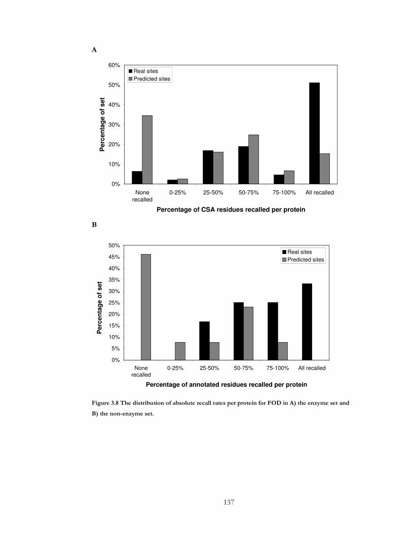
137

A

0%

10%

20%

30%

40%

50%

60%

None

recalled

0-25% 25-50% 50-75% 75-100% All recalled


Per

cen

tag

e o

f se

t

Real sites

Predicted sites

B

0%

5%

10%

15%

20%

25%

30%

35%

40%

45%

50%

Nonerecalled

0-25% 25-50% 50-75% 75-100% All recalled


Per

cen

tag

e o

f se

t

Real sites

Predicted sites

Figure 3.8 The distribution of absolute recall rates per protein for FOD in A) the enzyme set and

B) the non-enzyme set.

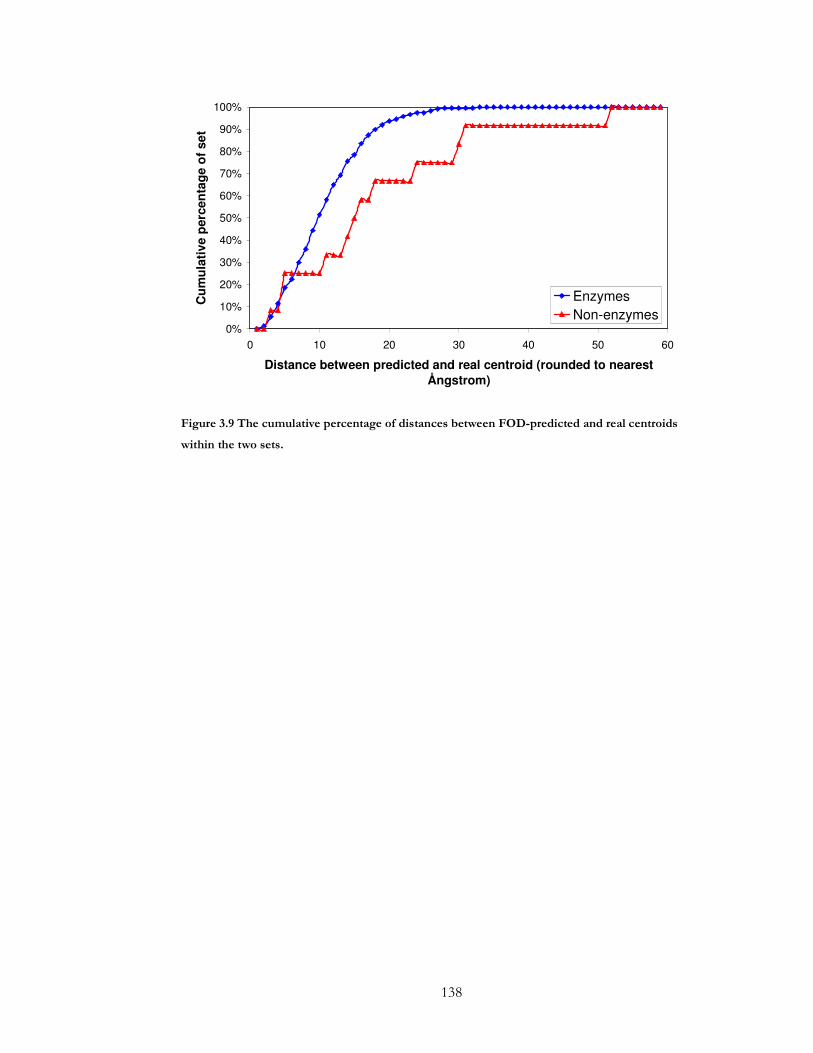
138

0%

10%

20%

30%

40%

50%

60%

70%

80%

90%

100%

0 10 20 30 40 50 60


Cu

mu

lati

ve p

erce

nta

ge

of

set

Enzymes

Non-enzymes

Figure 3.9 The cumulative percentage of distances between FOD-predicted and real centroids

within the two sets.

139

3.4.5 QSiteFinder

Method Description

QSiteFinder finds clefts on the proteins surface and then ranks them according to their

interaction energy between the protein and a van der Waals probe. Non-bonded

interaction energies are calculated by placing a 0.9Å 3D grid over the whole protein

and then evaluating the interaction energy between the protein and a methyl group at

each point on the grid. The positions of the probes on the grid that gave the best

interaction energies were then spatially clustered to identify groups of close probes.

These clusters are then assigned a single interaction energy based on the energies of

their member probes. The clusters are then ranked by their representative interaction

energy and the highest ranked cluster is predicted as the functional site. Protein residue

atoms that are in contact with the predicted site are given as the predicted functional

site residues. The output gives a list of ranked sites but only the top-ranking site will

be used for this analysis.

Prediction Accuracy

QSiteFinder gives output for multiple site predictions ranked in order of the likelihood

of being a real active site. For this analysis the first ranked predicted site is taken. For

each site, a set of atoms predicted as existing in the active site is given. Not all atoms

for a residue are predicted, but for consistentcy with other methods, if an atom of a

residue is given in the prediction the coordinates of the Cβ atom of that residue, even if

it is not given in the prediction, are used to calculate the centroid.

QSiteFinder can only process structures with less than 10,000 atoms and this excluded

24 proteins from the enzyme set and one from the non-enzyme set. For the remainder

of the enzyme dataset QSiteFinder achieved relative recall rate of 53.0% and 54.0% for

the non-enzyme set (see Table 3.9). Q-SiteFinder performed better than the CSA-

generated centroid for 1qd6 in the enzyme set. The QSiteFinder-generate centroid

recalled all 3 of the CSA annotated residues as opposed to the two recalled by the CSA-

generated centroid.

140

The distribution of percentage recall rates per protein for QSiteFinder compared to the

real sites are shown in Figure 3.10. QSiteFinder appears to get the prediction wrong

40% of the time in enzymes and ~30% of the time in non-enzymes. Just over 45% of

the predictions are within 10Ǻ of the real centroid in enzymes but almost 60% for non-

enzymes (Figure 3.11).

QSiteFinder Enzyme Set Non-enzyme

Set

Site Residue Recall












Table 3.9 The functional site prediction accuracy results for QSiteFinder

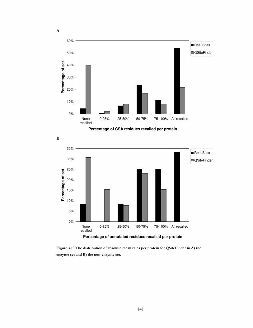
141

A

0%

10%

20%

30%

40%

50%

60%

Nonerecalled

0-25% 25-50% 50-75% 75-100% All recalled


Per

cen

tag

e o

f se

t

Real Sites

QSiteFinder

B

0%

5%

10%

15%

20%

25%

30%

35%

Nonerecalled

0-25% 25-50% 50-75% 75-100% All recalled


Per

cen

tag

e o

f se

t

Real Sites

QSiteFinder

Figure 3.10 The distribution of absolute recall rates per protein for QSiteFinder in A) the

enzyme set and B) the non-enzyme set.

142

0%

10%

20%

30%

40%

50%

60%

70%

80%

90%

100%

0 10 20 30 40 50 60


Cu

mu

lati

ve p

erce

nta

ge

of

set

Enzymes

Non-enzymes

Figure 3.11 The cumulative percentage of distances between QSiteFinder-predicted and real


143

3.4.6 PDBSiteScan

Method description

PDBSiteScan takes 3D fragments of a protein structure and compares them to 3D

structure fragments of known active sites. The known active sites structures are held in

a collection called PDBSite that is formed from annotation in the PDB SITE field and

also REMARK 800 fields. PDBSite stores several types of ‘functional’ sites including

protein-protein interactions and posttranslational modification sites. In the enzyme

analysis only the sites marked as “active sites” were searched.

The alignment of the site template and the test protein are performed using CE61

(Combinatorial Extension) and the N, C and Cα atoms are used to define the

orientation of the residue. For a template to match a 3D fragment the maximum

distance mismatch (MDM), the sum of the Cartesian distances between each atom in

the template and the fragment, has to be less than the user defined cut-off. In this

analysis the default setting of 2Å was used.

Prediction accuracy

PDBSiteScan was problematic to run and gave errors for 53 of the 237 structures in

the enzyme dataset. This included 19 structures where the protein found during the

scan of the PDB was the same as the query structure, 18 structures where the scan

could not find any similar proteins and a further 16 where PDBSiteScan did not run

due to other technical errors. It performed relatively poorly on the remaining enzyme

structures, giving a relative recall rate of 38.4% (see Table 3.10). PDBSiteScan could

not produce results for three of the non-enzyme structures and only produced a

relative recall rate of 23.5% for the non-enzyme set.

144

PDBSiteScan Enzyme Set Non-enzyme

Set

Site Residue Recall











Average percentage of site residues shared per protein 23.2% 15.0%

Table 3.10 The functional site prediction accuracy results for PDBSiteScan

The distribution of recall rates is shown in Figure 3.12 and the distance between

predicted and real site centroids is shown in Figure 3.13. PDBSiteScan appears to get

the prediction wrong over half of the time in both sets and with some degree of

accuracy the remaining time (Figure 3.12). Approximately only 30% and 20% of the

predictions are within 10Ǻ of the real enzyme and non-enzyme centroids, respectively

(Figure 3.13).

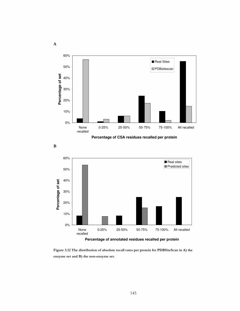
145

A

0%

10%

20%

30%

40%

50%

60%

None

recalled

0-25% 25-50% 50-75% 75-100% All recalled


Per

cen

tag

e o

f se

tReal Sites

PDBsitescan

B

0%

10%

20%

30%

40%

50%

60%

Nonerecalled

0-25% 25-50% 50-75% 75-100% All recalled


Per

cen

tag

e o

f se

t

Real sites

Predicted sites

Figure 3.12 The distribution of absolute recall rates per protein for PDBSiteScan in A) the


146

0%

10%

20%

30%

40%

50%

60%

70%

80%

90%

100%

0 10 20 30 40 50


Cu

mu

lati

ve p

erce

nta

ge

of

set

Figure 3.13 The cumulative percentage of distances between PDBSiteScan-predicted and real


147

3.4.7 Consurf

Method description

Consurf calculates the degree of evolutionary conservation for each residue in a

structure and assigns them an integer score from 1 to 9, with 9 being the most

conserved residues. A graphical representation of the structure is then coloured

according to these residue conservation scores, which allows visual identification of

highly conserved patches, which are predicted to be functional sites.

Prediction Accuracy

Consurf only accepts one chain as input to the method and so the first chain from the

structure file was used to obtain predictions. Where there are multiple copies of this

chain in the structure the predicted site annotation from the input chain is copied

across to all other identical chains. The primary output of this method is via a graphic

of the protein structure coloured according to the residues’ degree of conservation.

Visual inspection of this coloured structure allows the identification of surface patches

of highly conserved residues. This analysis however, requires output to be

automatically evaluated and therefore residues were taken as predicted site residues

when they were assigned the top conservation score (9).

Consurf did not produce output for 4 of the 237 proteins in the enzyme set and 3 of

the 13 proteins in the non-enzyme dataset. Despite only being able to predict sites for

one chain of a protein, Consurf achieved an average relative recall rate of 78.2% for

enzymes and 52.1% for non-enzymes (see Table 3.11). Around 70% of proteins had

predicted centroids within 10Å of the real centroid for both the enzyme and non-

enzyme set (see Figure 3.15).

148

Consurf Enzyme Set Non-enzyme

Set

Site Residue Recall












Table 3.11 The functional site prediction accuracy results for Consurf.

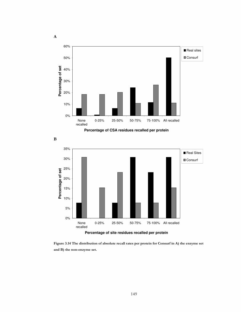
149

A

0%

10%

20%

30%

40%

50%

60%

Nonerecalled

0-25% 25-50% 50-75% 75-100% All recalled


Per

cen

tag

e o

f se

t

Real sites

Consurf

B

0%

5%

10%

15%

20%

25%

30%

35%

Nonerecalled

0-25% 25-50% 50-75% 75-100% All recalled

Percentage of site residues recalled per protein

Per

cen

tag

e o

f se

t

Real Sites

Consurf

Figure 3.14 The distribution of absolute recall rates per protein for Consurf in A) the enzyme set

and B) the non-enzyme set.

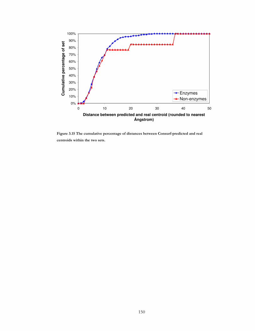
150

0%

10%

20%

30%

40%

50%

60%

70%

80%

90%

100%

0 10 20 30 40 50


Cu

mu

lati

ve p

erce

nta

ge

of

set

Enzymes

Non-enzymes

Figure 3.15 The cumulative percentage of distances between Consurf-predicted and real


151

3.4.8 Thematics

Method description

Thematics identifies ionisable residues with unusually perturbed titrations curves.

Active sites are predicted where two or more of these ionisable residues form a cluster

in 3D space. This method is only applicable to enzyme active sites, and therefore isn’t

assessed for the non-enzyme set.

Prediction accuracy

Thematics was unable to produce output for 25 of the 237 proteins in the enzyme set

and since Thematics is developed as an active-site predictor for enzymes, it was not

used n the non-enzyme dataset. Thematics achieved an average relative recall rate of

48.9% for enzymes (see Table 3.11 ) with around 40% of the predicted centroids being

within 10Å of the real centroid (see Figure 3.17).

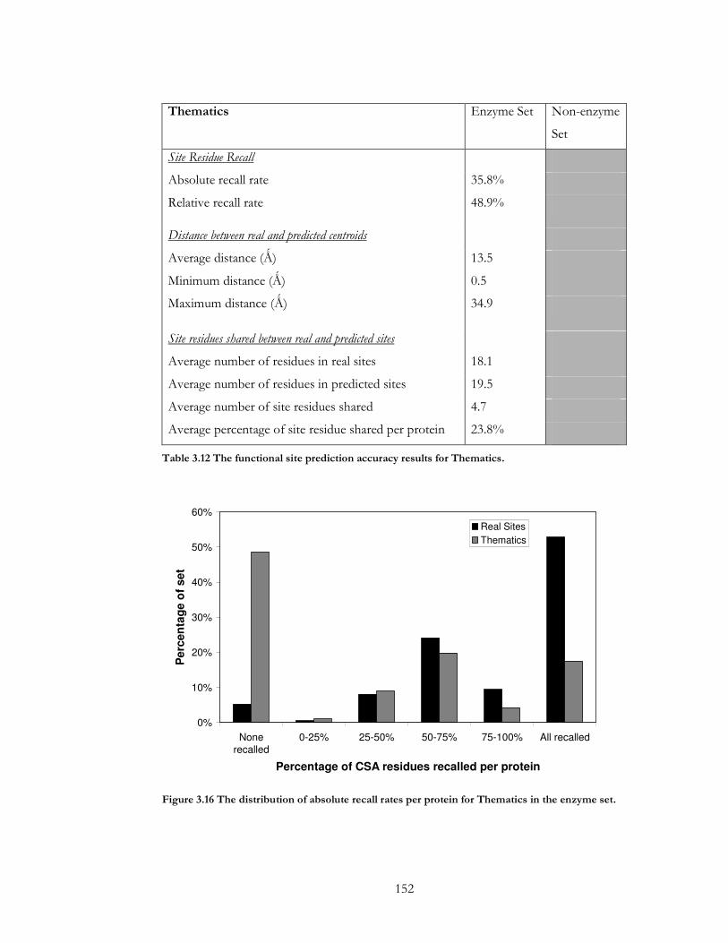
152

Thematics Enzyme Set Non-enzyme

Set

Site Residue Recall

Absolute recall rate 35.8%

Relative recall rate 48.9%


Average distance (Ǻ) 13.5

Minimum distance (Ǻ) 0.5

Maximum distance (Ǻ) 34.9


Average number of residues in real sites 18.1

Average number of residues in predicted sites 19.5

Average number of site residues shared 4.7

Average percentage of site residue shared per protein 23.8%

Table 3.12 The functional site prediction accuracy results for Thematics.

0%

10%

20%

30%

40%

50%

60%

Nonerecalled

0-25% 25-50% 50-75% 75-100% All recalled


Per

cen

tag

e o

f se

t

Real Sites

Thematics

Figure 3.16 The distribution of absolute recall rates per protein for Thematics in the enzyme set.

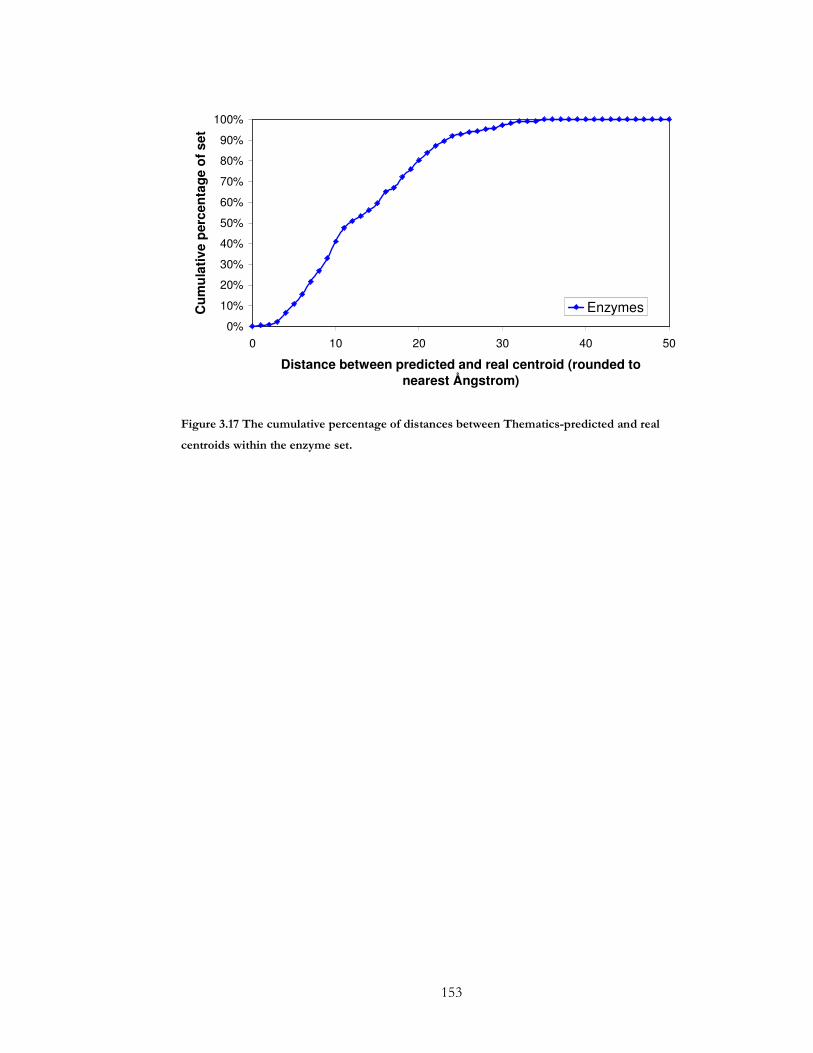
153

0%

10%

20%

30%

40%

50%

60%

70%

80%

90%

100%

0 10 20 30 40 50


Cu

mu

lati

ve p

erce

nta

ge

of

set

Enzymes

Figure 3.17 The cumulative percentage of distances between Thematics-predicted and real

centroids within the enzyme set.

154

3.4.9 SitesIdentify(GM) – Geometry-based

Method Description

The method behind SitesIdenitfy(GM) is explained in detail in 3.3.1 but in brief, a 2Å

grid is placed over the protein structure and a uniform charge is applied to each non-

hydrogen atom. The electrostatic potential is calculated using Finite Difference

Poisson-Boltzmann calculations with no dielectric boundary and the peak potential is

predicted as the centroid of the functional site.

Prediction Accuracy

SitesIdentify(GM) did not run successfully for two structures, 10o4 and 1rbl, but did

successfully produce output for the other 235. It achieved an average relative

percentage accuracy per protein of 63.0% for enzymes yet a higher accuracy of 69.5%

for non-enzymes (see Table 3.13). For 4 of the structures in the enzyme dataset, 1snn,

2sqc, 1qd6 and 1mvn, the SitesIdentify-generated centroid recalled one more CSA

annotated residue than the CSA-generated centroid.

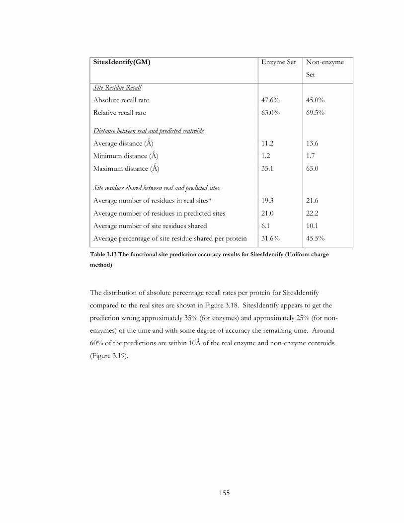
155

SitesIdentify(GM) Enzyme Set Non-enzyme

Set

Site Residue Recall








Average number of residues in real sites* 19.3 21.6




Table 3.13 The functional site prediction accuracy results for SitesIdentify (Uniform charge

method)

The distribution of absolute percentage recall rates per protein for SitesIdentify

compared to the real sites are shown in Figure 3.18. SitesIdentify appears to get the

prediction wrong approximately 35% (for enzymes) and approximately 25% (for non-

enzymes) of the time and with some degree of accuracy the remaining time. Around

60% of the predictions are within 10Ǻ of the real enzyme and non-enzyme centroids

(Figure 3.19).

156

0%

10%

20%

30%

40%

50%

60%

None

recalled

0-25% 25-50% 50-75% 75-100% All recalled


Per

cen

tag

e o

f se

t

Real Sites

SitesIdentify

0%

5%

10%

15%

20%

25%

30%

35%

40%

45%

None

recalled

0-25% 25-50% 50-75% 75-100% All recalled


Per

cen

tag

e o

f se

t

Real Sites

SitesIdentify

Figure 3.18 The distribution of absolute recall rates per protein for SitesIdentify(GM) in A) the


157

0%

10%

20%

30%

40%

50%

60%

70%

80%

90%

100%

0 10 20 30 40 50 60 70


Cu

mu

lati

ve p

erce

nta

ge

of

set

Enzymes

Non-enzymes

Figure 3.19 The cumulative percentage of distances between SitesIdentify(GM) predicted and

real centroids within the enzyme and non-enzyme set.

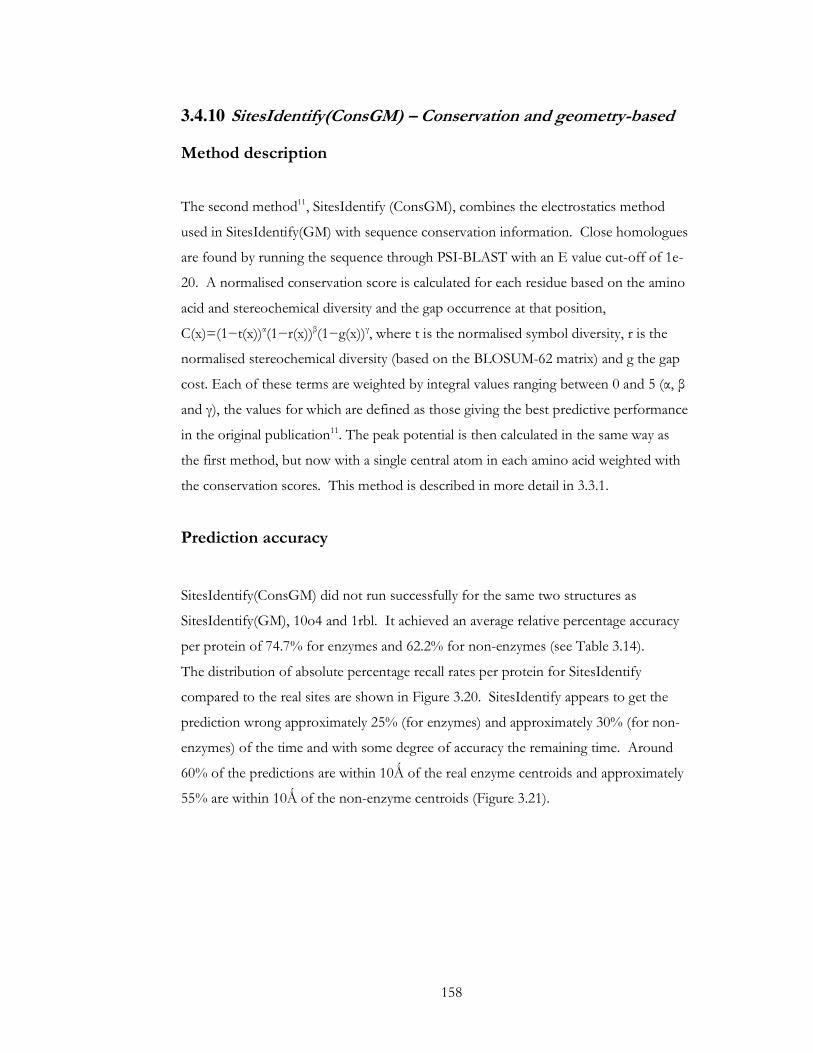
158

3.4.10 SitesIdentify(ConsGM) – Conservation and geometry-based

Method description

The second method11, SitesIdentify (ConsGM), combines the electrostatics method

used in SitesIdentify(GM) with sequence conservation information. Close homologues

are found by running the sequence through PSI-BLAST with an E value cut-off of 1e-

20. A normalised conservation score is calculated for each residue based on the amino

acid and stereochemical diversity and the gap occurrence at that position,

C(x)=(1−t(x))α(1−r(x))β(1−g(x))γ, where t is the normalised symbol diversity, r is the

normalised stereochemical diversity (based on the BLOSUM-62 matrix) and g the gap

cost. Each of these terms are weighted by integral values ranging between 0 and 5 (α, β

and γ), the values for which are defined as those giving the best predictive performance

in the original publication11. The peak potential is then calculated in the same way as

the first method, but now with a single central atom in each amino acid weighted with

the conservation scores. This method is described in more detail in 3.3.1.

Prediction accuracy

SitesIdentify(ConsGM) did not run successfully for the same two structures as

SitesIdentify(GM), 10o4 and 1rbl. It achieved an average relative percentage accuracy

per protein of 74.7% for enzymes and 62.2% for non-enzymes (see Table 3.14).

The distribution of absolute percentage recall rates per protein for SitesIdentify

compared to the real sites are shown in Figure 3.20. SitesIdentify appears to get the

prediction wrong approximately 25% (for enzymes) and approximately 30% (for non-

enzymes) of the time and with some degree of accuracy the remaining time. Around

60% of the predictions are within 10Ǻ of the real enzyme centroids and approximately

55% are within 10Ǻ of the non-enzyme centroids (Figure 3.21).

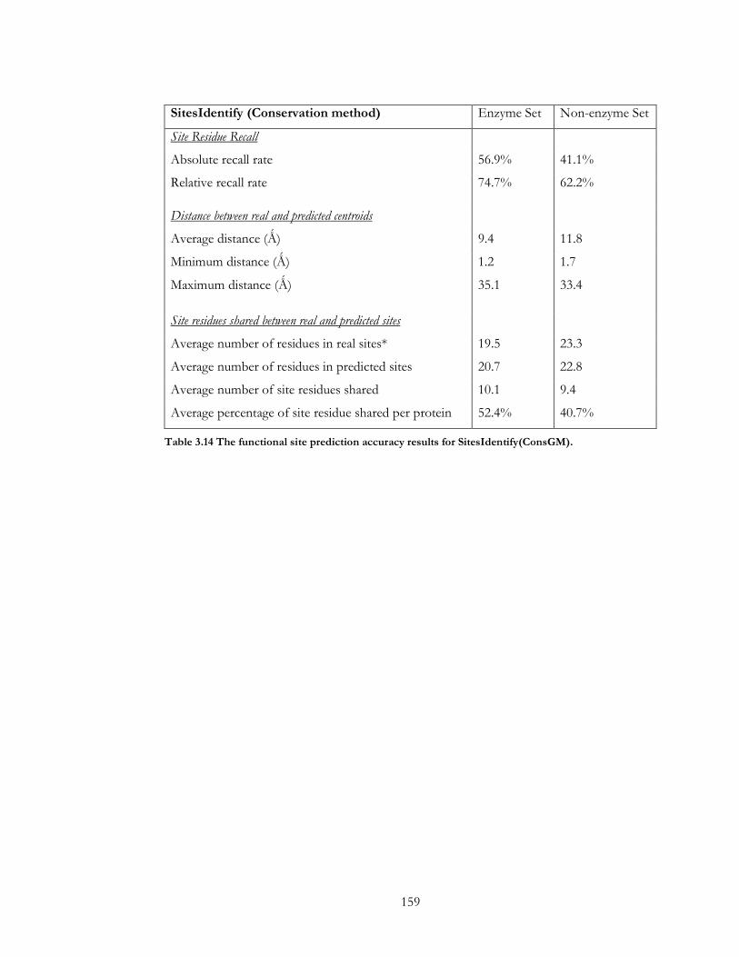
159

SitesIdentify (Conservation method) Enzyme Set Non-enzyme Set

Site Residue Recall








Average number of residues in real sites* 19.5 23.3




Table 3.14 The functional site prediction accuracy results for SitesIdentify(ConsGM).

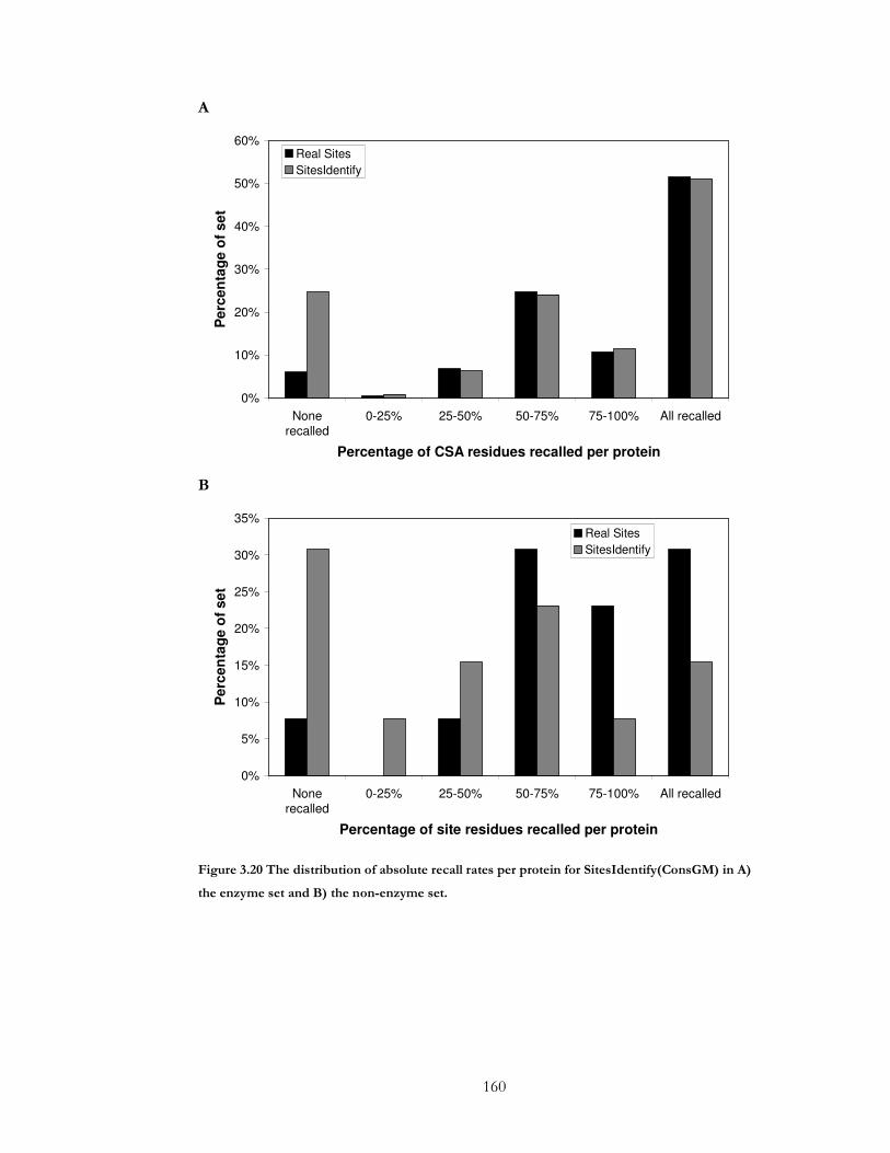
160

A

0%

10%

20%

30%

40%

50%

60%

Nonerecalled

0-25% 25-50% 50-75% 75-100% All recalled


Per

cen

tag

e o

f se

t

Real Sites

SitesIdentify

B

0%

5%

10%

15%

20%

25%

30%

35%

Nonerecalled

0-25% 25-50% 50-75% 75-100% All recalled


Per

cen

tag

e o

f se

t

Real Sites

SitesIdentify

Figure 3.20 The distribution of absolute recall rates per protein for SitesIdentify(ConsGM) in A)

the enzyme set and B) the non-enzyme set.

161

0%

10%

20%

30%

40%

50%

60%

70%

80%

90%

100%

0 10 20 30 40 50


Cu

mu

lati

ve p

erce

nta

ge

of

set

Enzymes

Non-enzymes

Figure 3.21 The cumulative percentage of distances between SitesIdentify(ConsGM) predicted

and real centroids within the enzyme and non-enzyme set.

3.4.11 All Methods

The absolute and relative recall rates of all methods are shown in Table 3.15 for the

enzyme set and Table 3.16 for the non-enzymes set. A comparison of the cumulative

percentages of the distances between predicted and real centroids between all methods

are shown in Figure 3.22 for enzymes and Figure 3.23 for non-enzymes. These show

that Consurf achieves the highest relative recall rate for enzymes with

SitesIdentify(GM) achieving the highest relative recall rate for non-enzymes.

162

0%

10%

20%

30%

40%

50%

60%

70%

80%

90%

100%

0 5 10 15 20 25 30 35 40 45 50

Distance between predicted and real centroid (rounded to nearest Angstrom)

Cu

mu

lati

ve p

erce

nta

ge

of

set

SitesIdentify (Geometry)SitesIdentify (Geometry + Conservation)FODQsitefinderCrescendoPDBsitescanPASSThematicsConsurf

Figure 3.22 Comparison of distances between the real centroids and the predicted centroids in

the enzyme dataset for each method.

0%

10%

20%

30%

40%

50%

60%

70%

80%

90%

100%

0 10 20 30 40 50 60


Cu

mu

lati

ve p

erce

nta

ge

of

set

SitesIdenitfy (Uniform charge method)

SitesIdentify (Conservation Method)

FOD

QSiteFinder

Crescendo

PDBSiteScan

PASS

Consurf

Figure 3.23 Comparison of distances between the real centroids and the predicted centroids in

the non-enzyme dataset for each method.

163

Method Absolute Recall Rate

Relative Recall Rate

Average Distance between Predicted and Real Centroid

(Å) SitesIdentify SitesIdentify(GM) 47.6% 63.0% 11.2 SitesIdentify(ConsGM) 56.9% 74.7% 9.4 Consurf 58.6% 78.2% 8.2 Crescendo 46.9% 63.8% 10.3 FOD 39.7% 56.1% 10.6 QSiteFinder 40.1% 53.0% 13.0 PDBSiteScan 28.1% 38.4% 15.5 PASS 36.6% 49.3% 14.8 Thematics 35.8% 48.9% 13.5

Table 3.15 The absolute and relative recall rates achieved for the enzyme dataset along with the

average distance between real and predicted centroids for each method.

Method Absolute Recall Rate

Relative Recall Rate

Average Distance between Predicted and

Real Centroid (Å) SitesIdentify SitesIdentify(GM) 45.0% 69.1% 13.6 SitesIdentify(ConsGM) 41.0% 62.2% 11.8 Consurf 36.3% 52.1% 13.1 Crescendo 44.2% 65.8% 11.8 FOD 22.9% 33.7% 18.1 QSiteFinder 33.6% 54.0% 12.5 PDBSiteScan 11.4% 23.5% 19.5 PASS 37.5% 47.1% 17.4

Table 3.16 The absolute and relative recall rates achieved for the non-enzyme dataset along with

the average distance between real and predicted centroids for each method.

Whilst achieving a slightly lower recall accuracy than Consurf, SitesIdentify(ConsGM)

also performs well for the enzyme dataset. Consurf, however, only makes predictions

for one chain of a structure and whilst this may be a limitation of the method, on this

dataset it had an advantageous effect on the recall accuracy for Consurf. Residues in a

structure can be conserved for either functional or structural reasons, and residues that

form a subunit interface may exhibit similar levels of conservation to functional

residues. Since SitesIdentify(ConsGM) identifies clusters of highly conserved residues,

it could be distracted from the functional site by a cluster of conserved residues at the

interface between two chains. Consurf would not be able to detect a cluster of

conserved residues between two chains as it only evaluates the degree of conservation

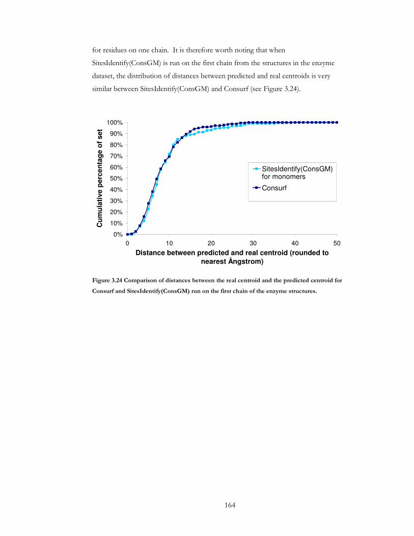
164

for residues on one chain. It is therefore worth noting that when

SitesIdentify(ConsGM) is run on the first chain from the structures in the enzyme

dataset, the distribution of distances between predicted and real centroids is very

similar between SitesIdentify(ConsGM) and Consurf (see Figure 3.24).

0%

10%

20%

30%

40%

50%

60%

70%

80%

90%

100%

0 10 20 30 40 50


Cu

mu

lati

ve p

erce

nta

ge

of

set

SitesIdentify(ConsGM)for monomers

Consurf

Figure 3.24 Comparison of distances between the real centroid and the predicted centroid for

Consurf and SitesIdentify(ConsGM) run on the first chain of the enzyme structures.

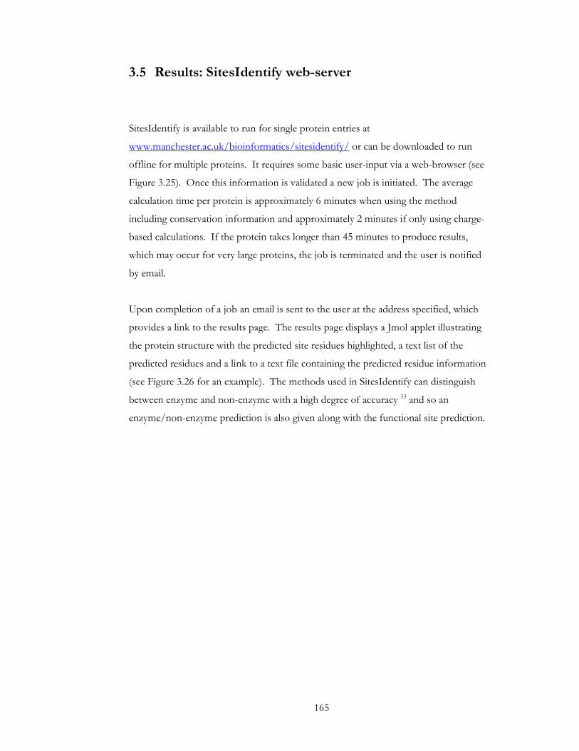
165

3.5 Results: SitesIdentify web-server

SitesIdentify is available to run for single protein entries at

www.manchester.ac.uk/bioinformatics/sitesidentify/ or can be downloaded to run

offline for multiple proteins. It requires some basic user-input via a web-browser (see

Figure 3.25). Once this information is validated a new job is initiated. The average

calculation time per protein is approximately 6 minutes when using the method

including conservation information and approximately 2 minutes if only using charge-

based calculations. If the protein takes longer than 45 minutes to produce results,

which may occur for very large proteins, the job is terminated and the user is notified

by email.

Upon completion of a job an email is sent to the user at the address specified, which

provides a link to the results page. The results page displays a Jmol applet illustrating

the protein structure with the predicted site residues highlighted, a text list of the

predicted residues and a link to a text file containing the predicted residue information

(see Figure 3.26 for an example). The methods used in SitesIdentify can distinguish

between enzyme and non-enzyme with a high degree of accuracy 33 and so an

enzyme/non-enzyme prediction is also given along with the functional site prediction.

166

Figure 3.25 Screenshot for SitesIdentify showing the required user input fields.

A user can either input a pre-existing PDB code and whether to use the asymmetric or

biological unit structure or upload their own PDB-style structure file. All fields are compulsory.

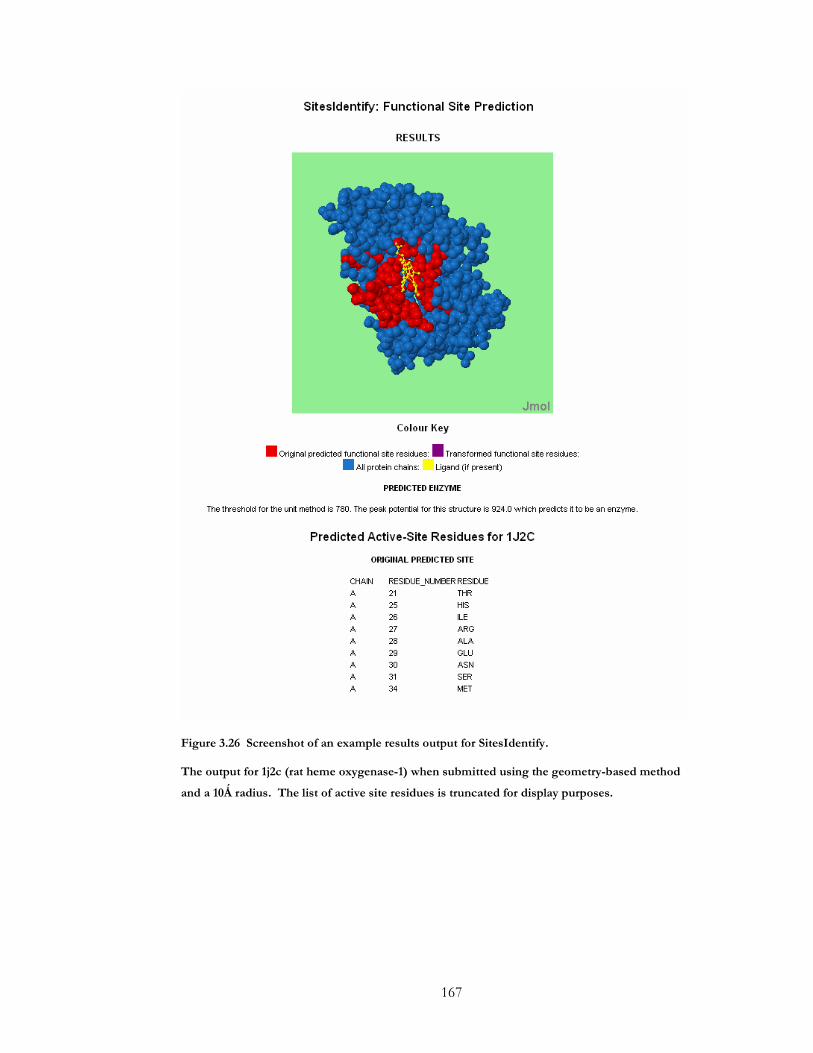
167

Figure 3.26 Screenshot of an example results output for SitesIdentify.

The output for 1j2c (rat heme oxygenase-1) when submitted using the geometry-based method

and a 10Ǻ radius. The list of active site residues is truncated for display purposes.

168

SitesIdentify only gives a prediction for a single functional site as it makes predictions

based on the single highest peak potential. In oligomeric structures, however, the same

site may be present in multiple subunits and so where there is a similar site in other

chains SitesIdentify identifies it as another possible site. These residues are highlighted

in purple on the protein structure (see Figure 3).

Figure 3.27 An example of highlighted residues in an alternative predicted site.

The biological unit structure for 2af4 (phosphotransacetylase) is a homodimer and identical

active sites are present on both chains. SitesIdentify identifies only one site (in red), but the

annotation is transformed onto the other chain in order to identify the other active site (shown

in purple).

Where a user inputs a pre-existing PDB ID to SitesIdentify, the option to use either the

asymmetric unit or the biological unit structure is given. Where the real functional site

is formed in or near subunit boundaries in the biological unit, running SitesIdentify on

the asymmetric unit may fail to give the correct prediction. Some biological units,

however, may give a false prediction particularly where there is an internal void formed

by a cyclical arrangement of subunits. Such voids tend to be well-buried, more so than

the real surface clefts, and the residues on the edges of these voids may be

169

evolutionarily conserved in order to retain the quaternary structure. These voids are

therefore sometimes incorrectly selected as predicted functional sites. Where a

biological unit has an internal void it would be useful to also run SitesIdentify on the

asymmetric unit. For example, running the asymmetric unit for 1B6T through the

SitesIdentify server locates the functional site in the correct location, however the site

is predicted incorrectly for the biological unit as the void formed in the centre of the

molecule (see Figure 3.28).

Figure 3.28 An example of differential site prediction between asymmetric and biological unit

structures.

The active site predicted for the asymmetric unit of 1b6t (phosphopantetheine

adenylyltransferase) is reasonably close to the bound ligand shown in part A. The biological

unit is formed by a cyclical arrangement of the asymmetric unit and when SitesIdentify is run

on this structure it incorrectly identifies the central void as the enzyme active site (part B).

170

3.6 Discussion

Both Consurf and SitesIdentify(ConsGM) are based around predicting conserved

residues as functional site residues but whilst Consurf appears to perform slightly

better overall, it could not produce predictions for three of the proteins in the set

(1C3J, 1DMU and 1PGS) as it was unable to identify enough homologues.

SitesIdentify(ConsGM) uses both a combination of residue conservation information

with an electrostatics-based cleft-finding algorithm and so still gives predictions where

there is little or no conservation information available. SitesIdentify was able to recall

100% of the annotated catalytic residues for the three proteins in this set for which

Consurf did not make any prediction. SitesIdentify, therefore, is likely to give better

predictions for structures from uncharacterised families, such as those being generated

by structural genomics initiatives.

In general, most methods perform better for predicting the functional sites of enzymes

than non-enzymes. The best-performing methods for the enzyme set, Consurf and

SitesIdentify(ConsGM), which both use conservation as a predictive feature are

overtaken by a non-conservation-based approach, SitesIdentify(GM) for the non-

enayme set. Residue conservation is known to be less indicative of functionality for

non-enzymes than for enzymes9,60,62. A study of four non-enzyme families by Magliery

et al. found that rather than binding sites being conserved, they showed a higher degree

of variation than the rest of the protein 9. This may explain why some conservation-

based methods, including those tested here (SitesIdentify and Consurf) and those not50;

62, report better accuracies in predicting functional sites of enzymes than non-enzymes.

It is therefore useful to the user if analysing a protein of unknown function to predict

whether the structure is an enzyme or non-enzyme when choosing which method of

SitesIdentify to use. Indeed, the webserver implementation of both SitesIdentify

methods includes an enzyme/non-enzyme prediction in the results output in order to

allow the user to select which method is likely to give the best functional site

prediction.

PDBSiteScan achieved the lowest absolute and relative recall rates (28.1% and 38.4%,

respectively) and also the largest average distance between predicted and real active-site

171

centroids (15.5Å). PDBSiteScan scans the query protein against proteins of known

annotation. In this analysis the test set consists of enzymes with known annotation and

therefore it was necessary to reject predictions that simply accessed the annotation of

any of these test proteins. As the number of proteins with well-characterised active site

information is limited, removing these proteins from the set that PDBSiteScan

compares to will obviously reduce the prediction power of the method. If tested on

proteins outside of this set (i.e. proteins with uncharacterised functional sites) the

prediction accuracy may increase.

Q-SiteFinder identifies energetically favourable methyl binding sites by calculating the

interaction energy between the protein and a methyl probe and then ranking clusters of

probes by their total interaction energy. Similar to the electrostatics-based method of

SitesIdentify, Q-SiteFinder is essentially a cleft-finding algorithm. Despite similar

approaches the uniform charge method of SitesIdentify achieves a 10% higher relative

recall rate than Q-SiteFinder. Both Q-SiteFinder and SitesIdentify performed better

than the other cleft-finding method, PASS, which also selects for cleft depth. Since

SitesIdentify implicitly detects the atom density around a cleft rather than the cleft

geometry itself, it suggests that this may be a contributing factor to the increased

accuracy over PASS.

It is interesting that whilst SitesIdentify(GM) and Crescendo use very different

approaches they give very similar accuracies on the enzyme dataset, suggesting that

both conservation and geometrical information are equally useful in identifying

functional sites. The combination of both of these approaches in

SitesIdentify(ConsGM) further improves the accuracy achieved by either one alone.

Both of the SitesIdentify methods are delivered as a publicly-available tool via a

webserver at www.manchester.ac.uk/bioinformatics/sitesidentify.

172

3.7 References

1. Bray, T., Chan, P., Bougouffa, S., Greaves, R., Doig, A. J. & Warwicker, J. (2009). SitesIdentify: a protein functional site prediction tool. BMC Bioinformatics 10, 379.

2. Capra, J. A. & Singh, M. (2007). Predicting functionally important residues from sequence conservation. Bioinformatics 23, 1875-82.

3. Manning, J. R., Jefferson, E. R. & Barton, G. J. (2008). The contrasting properties of conservation and correlated phylogeny in protein functional residue prediction. BMC Bioinformatics 9, 51.

4. Zhang, T., Zhang, H., Chen, K., Shen, S., Ruan, J. & Kurgan, L. (2008). Accurate sequence-based prediction of catalytic residues. Bioinformatics 24, 2329-38.

5. Fischer, J. D., Mayer, C. E. & Soding, J. (2008). Prediction of protein functional residues from sequence by probability density estimation. Bioinformatics 24, 613-20.

6. Liang, S., Zhang, C., Liu, S. & Zhou, Y. (2006). Protein binding site prediction using an empirical scoring function. Nucleic Acids Res 34, 3698-707.

7. Chelliah, V., Chen, L., Blundell, T. L. & Lovell, S. C. (2004). Distinguishing structural and functional restraints in evolution in order to identify interaction sites. J Mol Biol 342, 1487-504.

8. Berezin, C., Glaser, F., Rosenberg, J., Paz, I., Pupko, T., Fariselli, P., Casadio, R. & Ben-Tal, N. (2004). ConSeq: the identification of functionally and structurally important residues in protein sequences. Bioinformatics 20, 1322-4.

9. Magliery, T. J. & Regan, L. (2005). Sequence variation in ligand binding sites in proteins. BMC Bioinformatics 6, 240.

10. Caffrey, D. R., Somaroo, S., Hughes, J. D., Mintseris, J. & Huang, E. S. (2004). Are protein-protein interfaces more conserved in sequence than the rest of the protein surface? Protein Sci 13, 190-202.

11. Greaves, R. & Warwicker, J. (2005). Active site identification through geometry-based and sequence profile-based calculations: burial of catalytic clefts. J Mol Biol 349, 547-57.

12. Wang, K., Horst, J. A., Cheng, G., Nickle, D. C. & Samudrala, R. (2008). Protein meta-functional signatures from combining sequence, structure, evolution, and amino acid property information. PLoS Comput Biol 4, e1000181.

13. Ausiello, G., Zanzoni, A., Peluso, D., Via, A. & Helmer-Citterich, M. (2005). pdbFun: mass selection and fast comparison of annotated PDB residues. Nucleic Acids Res 33, W133-7.


15. Ivanisenko, V. A., Pintus, S. S., Grigorovich, D. A. & Kolchanov, N. A. (2005). PDBSite: a database of the 3D structure of protein functional sites. Nucleic Acids Res 33, D183-7.

173

16. Hulo, N., Bairoch, A., Bulliard, V., Cerutti, L., Cuche, B. A., de Castro, E., Lachaize, C., Langendijk-Genevaux, P. S. & Sigrist, C. J. (2008). The 20 years of PROSITE. Nucleic Acids Res 36, D245-9.

17. Torrance, J. W., Bartlett, G. J., Porter, C. T. & Thornton, J. M. (2005). Using a library of structural templates to recognise catalytic sites and explore their evolution in homologous families. J Mol Biol 347, 565-81.

18. Ivanisenko, V. A., Pintus, S. S., Grigorovich, D. A. & Kolchanov, N. A. (2004). PDBSiteScan: a program for searching for active, binding and posttranslational modification sites in the 3D structures of proteins. Nucleic Acids Res 32, W549-54.

19. Binkowski, T. A., Freeman, P. & Liang, J. (2004). pvSOAR: detecting similar surface patterns of pocket and void surfaces of amino acid residues on proteins. Nucleic Acids Res 32, W555-8.

20. Chang, D. T., Weng, Y. Z., Lin, J. H., Hwang, M. J. & Oyang, Y. J. (2006). Protemot: prediction of protein binding sites with automatically extracted geometrical templates. Nucleic Acids Res 34, W303-9.

21. Jambon, M., Andrieu, O., Combet, C., Deleage, G., Delfaud, F. & Geourjon, C. (2005). The SuMo server: 3D search for protein functional sites. Bioinformatics 21, 3929-30.

22. Kleywegt, G. J. (1999). Recognition of spatial motifs in protein structures. J Mol Biol 285, 1887-97.

23. Shulman-Peleg, A., Nussinov, R. & Wolfson, H. J. (2005). SiteEngines: recognition and comparison of binding sites and protein-protein interfaces. Nucleic Acids Res 33, W337-41.

24. Stark, A. & Russell, R. B. (2003). Annotation in three dimensions. PINTS: Patterns in Non-homologous Tertiary Structures. Nucleic Acids Res 31, 3341-4.

25. Kristensen, D. M., Chen, B. Y., Fofanov, V. Y., Ward, R. M., Lisewski, A. M., Kimmel, M., Kavraki, L. E. & Lichtarge, O. (2006). Recurrent use of evolutionary importance for functional annotation of proteins based on local structural similarity. Protein Sci 15, 1530-6.

26. Goyal, K., Mohanty, D. & Mande, S. C. (2007). PAR-3D: a server to predict protein active site residues. Nucleic Acids Res 35, W503-5.



29. Tang, Y. R., Sheng, Z. Y., Chen, Y. Z. & Zhang, Z. (2008). An improved prediction of catalytic residues in enzyme structures. Protein Eng Des Sel 21, 295-302.

30. Laskowski, R. A., Luscombe, N. M., Swindells, M. B. & Thornton, J. M. (1996). Protein clefts in molecular recognition and function. Protein Sci 5, 2438-52.

31. Gutteridge, A., Bartlett, G. J. & Thornton, J. M. (2003). Using a neural network and spatial clustering to predict the location of active sites in enzymes. J Mol Biol 330, 719-34.

32. Brady, G. P., Jr. & Stouten, P. F. (2000). Fast prediction and visualization of protein binding pockets with PASS. J Comput Aided Mol Des 14, 383-401.

33. Bate, P. & Warwicker, J. (2004). Enzyme/non-enzyme discrimination and prediction of enzyme active site location using charge-based methods. J Mol Biol 340, 263-76.

174

34. Elcock, A. H. (2001). Prediction of functionally important residues based solely on the computed energetics of protein structure. J Mol Biol 312, 885-96.

35. Ota, M., Kinoshita, K. & Nishikawa, K. (2003). Prediction of catalytic residues in enzymes based on known tertiary structure, stability profile, and sequence conservation. J Mol Biol 327, 1053-64.

36. Tong, W., Williams, R. J., Wei, Y., Murga, L. F., Ko, J. & Ondrechen, M. J. (2008). Enhanced performance in prediction of protein active sites with THEMATICS and support vector machines. Protein Sci 17, 333-41.

37. Dessailly, B. H., Lensink, M. F. & Wodak, S. J. (2007). Relating destabilizing regions to known functional sites in proteins. BMC Bioinformatics 8, 141.

38. Laurie, A. T. & Jackson, R. M. (2005). Q-SiteFinder: an energy-based method for the prediction of protein-ligand binding sites. Bioinformatics 21, 1908-16.

39. Wei, Y., Ko, J., Murga, L. F. & Ondrechen, M. J. (2007). Selective prediction of interaction sites in protein structures with THEMATICS. BMC Bioinformatics 8, 119.

40. Ondrechen, M. J., Clifton, J. G. & Ringe, D. (2001). THEMATICS: a simple computational predictor of enzyme function from structure. Proc Natl Acad Sci U S A 98, 12473-8.

41. Brylinski, M., Prymula, K., Jurkowski, W., Kochanczyk, M., Stawowczyk, E., Konieczny, L. & Roterman, I. (2007). Prediction of functional sites based on the fuzzy oil drop model. PLoS Comput Biol 3, e94.

42. Amitai, G., Shemesh, A., Sitbon, E., Shklar, M., Netanely, D., Venger, I. & Pietrokovski, S. (2004). Network analysis of protein structures identifies functional residues. J Mol Biol 344, 1135-46.

43. del Sol, A., Fujihashi, H., Amoros, D. & Nussinov, R. (2006). Residue centrality, functionally important residues, and active site shape: analysis of enzyme and non-enzyme families. Protein Sci 15, 2120-8.

44. Chea, E. & Livesay, D. R. (2007). How accurate and statistically robust are catalytic site predictions based on closeness centrality? BMC Bioinformatics 8, 153.

45. Ben-Shimon, A. & Eisenstein, M. (2005). Looking at enzymes from the inside out: the proximity of catalytic residues to the molecular centroid can be used for detection of active sites and enzyme-ligand interfaces. J Mol Biol 351, 309-26.

46. Cheng, G., Qian, B., Samudrala, R. & Baker, D. (2005). Improvement in protein functional site prediction by distinguishing structural and functional constraints on protein family evolution using computational design. Nucleic Acids Res 33, 5861-7.

47. Landgraf, R., Xenarios, I. & Eisenberg, D. (2001). Three-dimensional cluster analysis identifies interfaces and functional residue clusters in proteins. J Mol Biol 307, 1487-502.

48. Landau, M., Mayrose, I., Rosenberg, Y., Glaser, F., Martz, E., Pupko, T. & Ben-Tal, N. (2005). ConSurf 2005: the projection of evolutionary conservation scores of residues on protein structures. Nucleic Acids Res 33, W299-302.

49. Thibert, B., Bredesen, D. E. & del Rio, G. (2005). Improved prediction of critical residues for protein function based on network and phylogenetic analyses. BMC Bioinformatics 6, 213.

50. Glaser, F., Morris, R. J., Najmanovich, R. J., Laskowski, R. A. & Thornton, J. M. (2006). A method for localizing ligand binding pockets in protein structures. Proteins 62, 479-88.

51. SitesIdentify.

175

52. Bray, T., Doig, A. J. & Warwicker, J. (2009). Sequence and structural features of enzymes and their active sites by EC class. J Mol Biol 386, 1423-36.

53. Golovin, A. & Henrick, K. (2008). MSDmotif: exploring protein sites and motifs. BMC Bioinformatics 9, 312.

54. Altschul, S. F., Madden, T. L., Schaffer, A. A., Zhang, J., Zhang, Z., Miller, W. & Lipman, D. J. (1997). Gapped BLAST and PSI-BLAST: a new generation of protein database search programs. Nucleic Acids Res 25, 3389-402.

55. Lee, B. & Richards, F. M. (1971). The interpretation of protein structures: estimation of static accessibility. J Mol Biol 55, 379-400.

56. Stawiski, E. W., Mandel-Gutfreund, Y., Lowenthal, A. C. & Gregoret, L. M. (2002). Progress in predicting protein function from structure: unique features of O-glycosidases. Pac Symp Biocomput, 637-48.

57. Rose, G. D. & Roy, S. (1980). Hydrophobic basis of packing in globular proteins. Proc Natl Acad Sci U S A 77, 4643-7.

58. Jones, S. & Thornton, J. M. (1997). Analysis of protein-protein interaction sites using surface patches. J Mol Biol 272, 121-32.

59. Eisenberg, D., Schwarz, E., Komaromy, M. & Wall, R. (1984). Analysis of membrane and surface protein sequences with the hydrophobic moment plot. J Mol Biol 179, 125-42.

60. Kyte, J. & Doolittle, R. F. (1982). A simple method for displaying the hydropathic character of a protein. J Mol Biol 157, 105-32.

61. Shindyalov, I. N. & Bourne, P. E. (1998). Protein structure alignment by incremental combinatorial extension (CE) of the optimal path. Protein Eng 11, 739-47.

62. Burgoyne, N. J. & Jackson, R. M. (2006). Predicting protein interaction sites: binding hot-spots in protein-protein and protein-ligand interfaces. Bioinformatics 22, 1335-42.

176

Chapter 4: Predicting EC class from

enzyme structure

The aim of this work is to be able to predict protein function from structural and

sequence features without transferring functional annotation from homologous

proteins. Here, this relates to the prediction of top EC classes from the structural

features of a group of structurally non-homologous enzymes. Two prediction models

are presented in this chapter, one developed on a set of enzymes with known active site

locations and another on a larger set of enzymes that may, or may not, have known

active site locations. The former prediction method was included, along with the work

in Chapter 2, in a published article in J. Mol. Biol1.

4.1 Introduction

The importance of being able to predict protein function from structure (or sequence)

is reflected in the growing number of structures in the PDB2 that have little or no

annotation. It is estimated that between 1% and 3% of the structures in the PDB3,4

and approximately 40% of the sequences in GenBank3 have an ‘unknown function’

annotation. These are conservative estimates since many proteins are tentatively

assigned functions, or vague annotation, based on similarity to others. The rate at

which proteins structures are being solved is higher than the capacity for experimental

groups to characterise them. This has led to the rise in the number of protein

structures lacking functional annotation and presents a requirement for automatic

annotation methods.

Traditional methods to automatically predict protein function have centered around

transferring annotation from a characterised homologue. It is, however, one of the

aims of structural genomics initiatives to resolve proteins that may occupy more

remote areas of protein fold space. This has increased the number of structures for

which a functionally annotated homologue cannot be reliably identified. This has

produced a subset of functionally uncharacterized proteins for which tradition

177

similarity-based methods fail and therefore the need for methods that do not rely on

identifying a homologue has arisen.

A number of approaches exist to predict protein function from sequence or structure

in the absence of homology. Sequence features, such as hydrophobicity, polarity and

polarisability, have been used to predict classes of metal binding proteins5, lipid binding

proteins6, RNA binding proteins7 and enzyme8 and other function classifications9

without the inference of homology to other proteins.

Other approaches have included structural features to predict protein function. Within

a study of structural features of the proteases, Stawiski et al. found that they exhibit

similar characteristics such as smaller than average surface areas and higher Cα

densities, regardless of whether or not they were evolutionarily related10. They also

showed different secondary structure content to the non-proteases. By using these

features in a machine learning approach they were able to define a set of structural

classifiers that could predict whether a protein is a protease or non-protease with an

accuracy of over 86%. In a later study, Stawiski et al. also reported structural features

that are characteristic of the O-glycosidases such as distinctive electrostatic properties

of the proteins surface, despite differences in the overall fold11.

Previous work 12 has shown that the use of structural features of proteins in a machine

learning method can predict the top EC classification of an enzyme. It is hypothesised

that to further improve these methods, structural features specifically relating to a

protein’s functional site, such as active site specific amino acid compositions and

secondary structure content, may increase the prediction power of this method

178

4.1.1 Machine Learning Theory

Machine learning is a computational method that exploits relationships between

variables in datasets to make predictions about further outcomes. These outcomes, for

example, can be associations (i.e. predicting whether a customer X is likely to buy

product B based on them having bought product A) or classifications (predicting the

socio-economic group of customer X based on the features of their purchases). Most

machine learning methods take advantage of the underlying probability distributions of

feature values and can identify complex patterns in large datasets that are not easily

detectable without the use of such methods.

A vast number of machine learning approaches have been proposed, which fall broadly

into a number of categories; supervised, unsupervised, semi-supervised and

reinforcement learning. Supervised learning occurs when the input data for the

training set is labeled with the correct outcomes. The machine learning method then

derives classification rules based on the observed relationships between the feature

values and the true classification. These rules are then used to predict an outcome

based upon an unlabeled test case. In contrast, unsupervised machine learning

methods do not require the input training data to be labeled with the correct outcome.

Instead, feature values are used to cluster the data into sets of similar cases with some

optimum separation. The rules used to cluster this data are then used to identify a

cluster given a new test case.

Semi-supervised learning is a compromise between the two above methods, where the

training data contains a mixture of labeled and unlabeled data. The labeled data can be

used to seed or guide the clustering algorithm used to separate the unlabeled data.

Reinforcement machine learning methods assess the outcomes of sets of action

sequences to generate a new sequence of actions that are likely to yield a given

outcome, regardless of the outcome of individual actions. This type of machine

learning is often used on game-playing type applications where there are multiple

routes to a successful outcome with complex dependencies between actions.

179

The work described in this chapter lends itself to supervised learning since a large

number of enzyme structures are available with known classification labels (EC

numbers). There are a number of issues and limitations attached to using supervised

learning methods. Firstly, the size of the dataset is important to the outcome of

supervised learning methods. Only very simple classification functions can be learnt

from a small dataset and so complex classification functions require large datasets. The

ability of a method to find the correct classification function therefore depends on the

availability of suitable data.

The number of input variables (features) in the training (and test) dataset also has a

large impact on the accuracy of supervised learning models. Large numbers of features

increase the dimensionality that the method must use to find a suitable classifier and so

increase the complexity of the problem. The optimal classifier tends to be formed

from only a subset of the total features. Incorporating irrelevant features into a model

makes it too detailed to be accurate on more general datasets and can be prevented by

removing features from the dataset using a feature selection algorithm.

It is important in all supervised learning methods that both the training set and the test

set are non-redundant, both within the sets and across the sets. If the same, or highly

similar, cases exist in the training set then the classifier will be skewed towards

classifying on the feature values from the overrepresented set of cases despite this bias

not being present in the test population. Similarly, if redundancy exists within the test

set then the accuracy will be either artificially enhanced or reduced depending on

whether that set of redundant cases are predicted correctly by the model or not. If

redundancy exists between the test and the training set then it will result in a classifier

that matches test cases to the training cases rather than forming a classifier that is

representative of the features that describe the classes.

The degree of heterogeneity in the data also can affect supervised learning methods.

Some supervised learning methods find it difficult to handle data where values of

features are on different scales to each other (or the dataset contains both continuous

and discrete data). Attributes that have small absolute values will exhibit smaller

absolute variance in their values and may be overshadowed by a higher absolute, but

smaller relative, variance in an attribute with a larger absolute value. Decision trees

180

(where a classifier is obtained using a series of binary rules to split the data) can handle

heterogeneity in the data well, but other methods such as linear regression and support

vector machines need to have each of their features scaled in a consistent manner

(usually -1 to 1 or 0 to 1) to reduce this bias.

There are a wide range of algorithms available that use supervised learning methods,

however a support vector machine (SVM) approach is used in the second prediction

method in this analysis. SVMs have been widely used in bioinformatics prediction

problems with success5-9,12,13 and are capable of high prediction accuracies.

4.1.1.1 Support Vector Machines

The SVM model can be thought of as representing a set of points in high dimensional

space, which are orientated according to their attributes. The model attempts to

identify a hyperplane that separates these points into their labeled classifications. The

optimum hyperplane is the one that separates the data into each class with the largest

distance between the hyperplane and the nearest points in each class (see Figure 4.1 for

a schematic representation). The ability for this method to find the optimum solution

quickly, by finding the hyperplane that divides the groups with the largest gap (i.e.

maximizing the margin between them) is one of the major advantages of this method.

Other approaches may identify a solution that separates the data, but not necessarily

the optimum and most general classifier and hence are susceptible to finding local

minima.

181

Figure 4.1 A schematic diagram representing the classification of two groups of data by an SVM

model.

Whilst the hyperplane A separates the data correctly the distance between the nearest points to

hyperplane A in each group (represented by grey dotted lines) is smaller than that of an

alternative hyperplane, B. The nearest points to the hyperplane (those that delimit the

maximum margin between the points and the hyperplane) are termed the support vectors.

Figure 4.1 represents a linear classifier, where cases can be separated by a linear

function. On real-world problems it is not often possible to separate the data using a

linear function and a technique called the kernel trick needs to be used. This maps the

points to a higher-dimensional space in order to achieve a separation by a hyperplane

with a linear function (see Figure 4.2).

182

Figure 4.2 A schematic diagram representing how the transformation of data into a higher-

dimensional space by using kernel functions can allow the separation of the data by a linear

function.

SVMs are binary classifiers and so need to be modified in order to classify into more

than two groups. One way of doing this is by conducting binary classifications

A

B

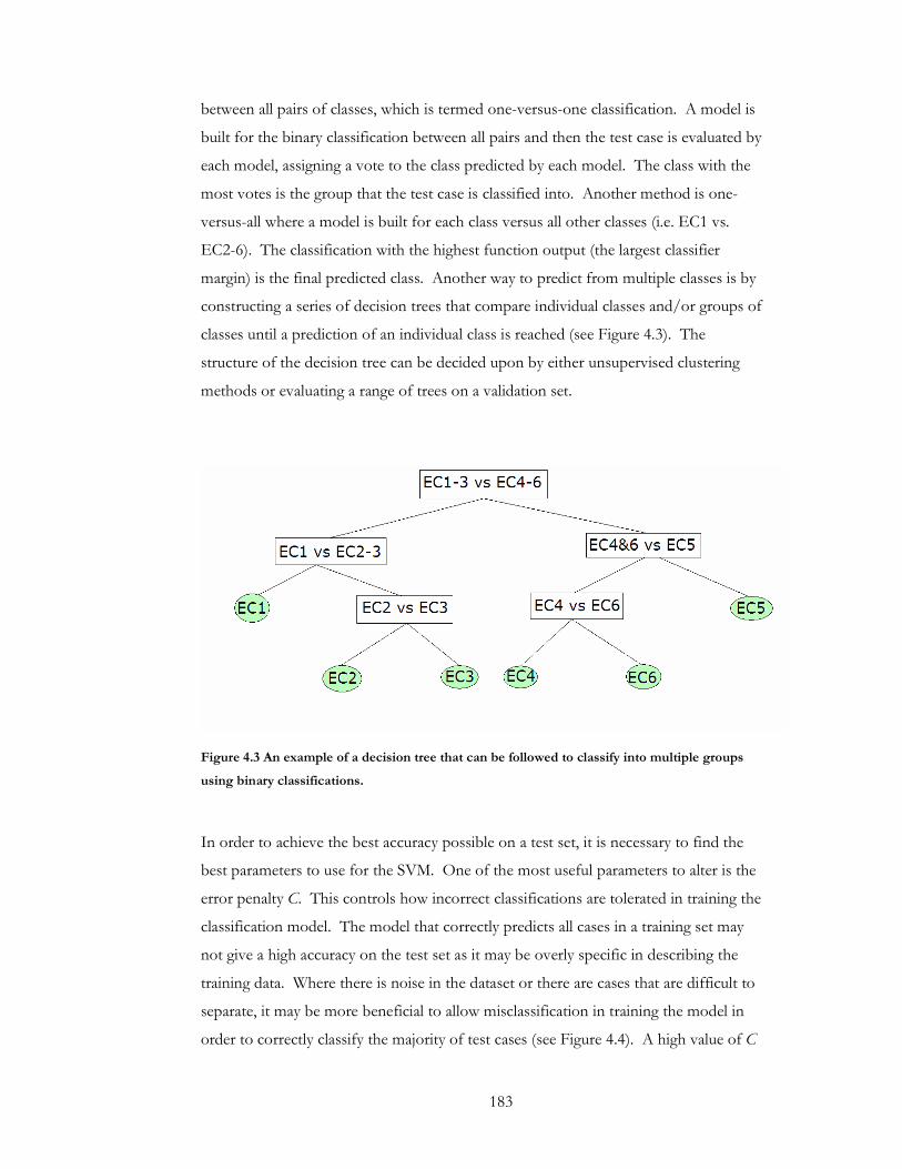
183

between all pairs of classes, which is termed one-versus-one classification. A model is

built for the binary classification between all pairs and then the test case is evaluated by

each model, assigning a vote to the class predicted by each model. The class with the

most votes is the group that the test case is classified into. Another method is one-

versus-all where a model is built for each class versus all other classes (i.e. EC1 vs.

EC2-6). The classification with the highest function output (the largest classifier

margin) is the final predicted class. Another way to predict from multiple classes is by

constructing a series of decision trees that compare individual classes and/or groups of

classes until a prediction of an individual class is reached (see Figure 4.3). The

structure of the decision tree can be decided upon by either unsupervised clustering

methods or evaluating a range of trees on a validation set.

Figure 4.3 An example of a decision tree that can be followed to classify into multiple groups

using binary classifications.

In order to achieve the best accuracy possible on a test set, it is necessary to find the

best parameters to use for the SVM. One of the most useful parameters to alter is the

error penalty C. This controls how incorrect classifications are tolerated in training the

classification model. The model that correctly predicts all cases in a training set may

not give a high accuracy on the test set as it may be overly specific in describing the

training data. Where there is noise in the dataset or there are cases that are difficult to

separate, it may be more beneficial to allow misclassification in training the model in

order to correctly classify the majority of test cases (see Figure 4.4). A high value of C

184

increases the penalty cost of creating a model that misclassifies examples and therefore

may produce a model that overfits the data. If the penalty is too low then the model

may misclassify too many examples and produce a model which is not meaningful.

Where non-linear kernel functions are used to generate the model, it may be useful to

optimise the values of kernel parameters. The γ parameter in the radial basis function

(RBF), a function whose value depends only on the distance from origin, specifies the

flexibility of the function. A high value of γ enables the kernel to closely fit the

separation of the training data and therefore may cause overfitting, whereas a small

value of γ may over generalise the model. Optimal values for each of these parameters

vary according to the classification problem and should be searched in order to identify

the best parameter values.

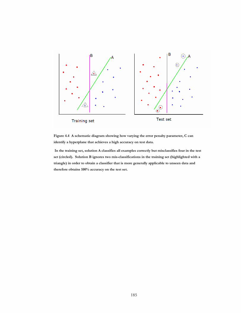
185

Figure 4.4 A schematic diagram showing how varying the error penalty parameter, C can

identify a hyperplane that achieves a high accuracy on test data.

In the training set, solution A classifies all examples correctly but misclassifies four in the test

set (circled). Solution B ignores two mis-classifications in the training set (highlighted with a

triangle) in order to obtain a classifier that is more generally applicable to unseen data and

therefore obtains 100% accuracy on the test set.

186

4.2 Methods

4.2.1 Dataset Creation

There are two datasets used in this chapter. Firstly, a prediction method is created that

uses features of known active sites and hence uses a dataset of enzymes with known

active sites (Dataset 4.1). Secondly, a prediction method is developed for enzymes

where the location of the active site is not known, and so enzymes without known

active site locations are introduced to the dataset (Dataset 4.2).

For the first method, the same dataset as in Chapter 2 was used. The creation of the

dataset is explained in detail in 2.2.1 and 2.3.1. In brief, the redundancy cull involves

ranking each enzyme in each class by descending AEROSPACI14 score and removing

any lower-ranked enzymes that share a domain from the same SCOP15 superfamily as

the domain containing the active site.

Dataset 4.2 was created in a similar manner as Dataset 4.1, however instead of using

enzymes that have known active site locations in the Catalytic Sites Atlas (CSA16)

Dataset 4.2 originates from all enzymes in the PDB that have a biological unit file. If

the PDB file contains an EC annotation then the top EC number is assigned to the

PDB. In the case where there is more than one EC classification for one PDB file the

enzyme is added to all classes for which there is annotation. If there is no EC number

in the PDB file, its corresponding Uniprot17 entry is searched for EC annotation. The

protein is assumed to be a non-enzyme if there is no EC annotation in either the PDB

file or the Uniprot entry. These non-enzymes are then checked manually to identify

any obvious omissions in EC number allocation (here, there were 105 cases of enzymes

that had to be manually annotated with an EC number). If the words “putative”,

“hypothetical”, “predicted”, “similarity”, “unknown” or “not known” were found in

the function comment line of the Uniprot entry then the corresponding PDB was

discarded as its function may not be certain.

187

4.2.2 Defining Active Site Residues

In order to include active site features to use in the prediction method, the active site

residues must first be defined. For Dataset 4.1 the location of the catalytic residues

(and hence the active site) are known but for Dataset 4.2 the active site residues must

be predicted.

4.2.2.1 Dataset 4.1

The methods for defining active site features for Dataset 4.1 are described in detail in

2.2.2. Briefly, the geometric average is calculated from the coordinates of the Cβ atom

(or Cα for glycine) of the catalytic residues listed in the CSA. This is termed the

centroid. All residues that have at least one atom within a 10Å radius of the centroid

and that have at least 5Å2 of solvent-accessible surface area (SASA) are defined as

active site residues.

4.2.2.2 Dataset 4.2

As the location of the active site is not known for all enzymes in this set, its location is

predicted using the SitesIdentify(ConsGM) method described in 3.3.1 and 3.4.10. This

prediction method gives XYZ coordinates relating to the central point in the predicted

active site of a PDB structure. In the same way as for Dataset 4.1, active site residues

are defined as any residue which has at least one atom within a 10Å radius of this

centroid and have at least 5Å2 of SASA.

4.2.3 Calculating Features.

The list of features that are calculated for these prediction methods are given in Table

4.1. For features listed as “Total” the feature is calculated using the whole sequence or

structure (the biological unit structure) and active site features are calculated using only

the active site residues as defined above. For sequence features the sequence given in

the SEQRES entry in the PDB file is used.

188

Feature Active site (AS), Total (T), Surface (S)

Structural features

Surface area AS/T Relative active site surface area AS Secondary structure content AS/T Average atomic B-factor Relative active site B-factor

AS/T AS

Oligomeric status (number of chains) T Number of residues in the biological unit T Molecular weight T

Sequence features

Sequence length T Amino acid composition (for all 20 amino acids) AS/T/S Polar/Non-polar/Negative/Aromatic/Positive proportions

AS/T

Average hydrophobicity (Kyte Doolittle score) AS/T Average isoelectric point (pI) AS/T Low complexity regions* T Table 4.1 Features used in the EC class prediction methods.

* Low sequence complexity was recorded in the form of three features; a binary feature that

recorded whether a low complexity region was identified or not and, if so, the number of low

complexity regions and the total length of the low complexity sequence(s).

4.2.3.1 Structural Features

Solvent-accessible surface area was calculated by an in-house program SACALC (J.

Warwicker), which rolls a solvent probe around the surface of the proteins to estimate

the amount of surface area (Å2) that is accessible to the probe. The relative active site

surface area is the proportion of the total surface area that is contributed to by the

active site residues. Secondary structure states for each residue were taken from the

secondary structure annotation from the PDB file, which is generated by a program

that incorporates DSSP18 and Promotif19. The average atomic B-factor is calculated by

averaging the atomic B-factors over all atoms in the protein (or active site). The

relative atomic B-factor for the active site is calculated by dividing the active site

average B-factor by the total average B-factor. The molecular weight of each enzyme

was calculated by the Pepstats program, which is part of the EMBOSS package of

applications20.

189

4.2.3.2 Sequence Features

Active site amino acid compositions were calculated by dividing the number of each

residue type in the active site residues by the total number of residues in the active site.

Total amino acid composition and surface amino acid composition were calculated

similarly, either using all residues or only those with at least 5Å2 surface area

respectively.

The polarity/charge fractions were calculated by dividing the number of residues from

each group (in either the total biological unit or the active site) by number of residues

in the biological unit or active site.

Average hydrophobicity values were obtained by dividing the sum of the Kyte &

Doolittle21 values for each residue in the protein (or in the active site) by the number of

residues in the protein (or in the active site). The polar amino acids contained the

positively charged (R, H, K), negatively charged (D, E) and uncharged amino acids (N,

Q, S, T). The non-polar amino acids were represented by the aromatic amino acids (F,

W) and non-polar amino acids (G, A, V, L, I, P, M). Cysteine and Tyrosine were not

included as they can be either polar or non-polar depending on the pH of the

environment.

The isoelectric point (pI) of a protein is the pH at which the protein has a net electrical

charge of zero. The pI of each enzyme was calculated by the Pepstats program, which

is part of the EMBOSS package of applications20. Low complexity regions were

predicted using SEG, a program that identifies low complexity regions in sequences22.

190

4.2.4 Prediction Methods

4.2.4.1 Functional Classification where the Active Site is

Known.

The classification tool is built around the principle of comparing a vector of the feature

values for each protein to vectors of average values for each functional class. Variation

in features with small values, such as the active site tyrosine proportion, cannot be

compared to the variation achievable for features with larger values, such as surface

area. The values for each feature were therefore normalised on a scale from 0 to 1 to

reduce the bias caused by features with larger absolute values. The minimum value for

a feature over the whole set is set to 0 and the maximum set to 1 and values in between

are linearly scaled accordingly.

In order to avoid bias by allowing the classification tool to use information from the

test enzyme in the class-average vector, a leave-one-out analysis was carried out. Each

enzyme was iteratively removed from the set and the class-average vectors were

formed from the class average of each feature for the remaining enzymes. The vector

formed from feature values for the test protein was then compared to each class

average vector and the angle between them calculated with a scalar product (see Figure

4.5). The closest class-average vector to the test enzyme vector (the pair giving the

smallest angle between them), represented the functional class predicted for the test

enzyme.

To reduce the effects of overfitting by using all features in the prediction model, each

feature’s contribution to the accuracy was evaluated. The accuracy achieved using all

features was obtained, then each feature was removed individually and the effect on the

accuracy observed. If the accuracy decreased when a feature was removed then the

feature was deemed to contribute positively to the prediction model and vice versa.

Features were then ranked by their individual contribution to the prediction model and

the prediction accuracy was iteratively assessed using increasing top n-ranked features.

The top n-ranked features that gave the highest accuracy were used as the features for

the final prediction model.

191

Figure 4.5 A schematic representation of the vector comparison method used to predict the EC

class of enzymes with known active sites.

The cosine of the angle between two vectors can be obtained by the scalar product of the

vectors (a and b, where a is the test enzyme and b is the class average vector). The class vector

that gives the smallest angle θ (or the largest cosine θ) between itself and the test protein vector

is the class predicted.

192

4.2.4.2 Functional Prediction where the Active Site is not

Known

The classification method used to predict the enzyme class of enzymes without a

known active site location was created using a support vector machine learning package

called LIBSVM23. Firstly each feature in the set was scaled between 0 and 1, where the

lowest value observed for that feature was set to 0 and the highest value was set to 1.

The dataset (Dataset 4.2) was then randomly split into a training and a test set, which

contains 625 (90%) and 70 (10%) enzymes, respectively.

The default kernel used in LIBSVM is the radial basis function (RBF), which is used in

this analysis as it can handle classifiers that are not linearly associated with each group.

LIBSVM also has an internal function to handle multi-class classification problems,

which is based on a one-against-one algorithm. Each class is compared against all

other classes and a model for the binary classification between each pair is constructed.

Each test case is then evaluated by each model and a vote is assigned to the class

predicted by each of the models. The class receiving the maximum number of votes is

the one assigned to that test case.

Two of the most influential factors when training a machine learning algorithm are the

parameters used and the features used. As discussed in the introduction, the error

penalty parameter, C, and the kernel parameter, γ, can be varied to identify the values

that give the optimum prediction performance. LIBSVM provides a grid-searching

algorithm that searches a range of C and γ values (the default is log2-5 to log213 for C

and log2-15 to log23 for γ). The performance of each pair of parameters was evaluated

using 10-fold cross-validation on the training set and the parameter values giving the

best accuracy were recorded.

The dataset used in this analysis is unbalanced in that the class sizes are very different

(for example the largest class, EC3, has over 5 times as many enzymes as EC6). This

imbalance in class sizes can result in the predictions being dominated by the largest

classes. LIBSVM provides an option to weight the error penalty for each class in order

to penalise predictions from larger classes more than those from smaller classes in

193

order to balance the predictions. Here, the error penalty parameter C is inversely

weighted by the ratios of the class sizes relative to the largest.

The second biggest contributor to the effectiveness of a machine learning model is the

features used. Using too many features in a machine learning method can be

detrimental for two reasons; 1) features that do not contain information relating to the

classes can distract the model from using more meaningful features and 2) using too

many features can lead to overfitting. Overfitting occurs when a very detailed model is

built and optimised for a training set using a large number of features. This detailed

model will give good accuracy on cross-validation evaluation on the dataset, since it

accurately describes the data within it. When this detailed model is used on data

outside of this training set the intricacies that described the training data well may

hinder the model. Removing features from the model will increase the ability for the

model to generalise and therefore produce better accuracy on unseen data.

A backward-pruning method was used here to remove features that negatively

impacted on the prediction model in the same way as described in 4.2.4.1. The features

were ranked according to their usefulness to the model and the number of top-ranked

features that gave the best cross-validation prediction accuracy on the dataset were

retained. These features, along with the optimum parameters values found in the grid

search were used to create a model on the training dataset, which was then used to

classify the unseen data in the test set.

194

4.3 Predicting EC class for Enzymes with Known Active

Site Location

A leave-one-out classification of each enzyme in the dataset into a top EC class using

all features achieved an accuracy of 29.1%. Each feature was then individually

removed and the effect on the prediction accuracy was observed. If the accuracy

decreases on removal of a feature it is deemed to have contributed positively to the

prediction model. The features were then ranked according to how much they had

contributed to the prediction accuracy. The prediction accuracy was assessed using an

increasing number of top n-ranked features. The highest accuracy (33.1%) was

achieved using the 74 top-ranked features (see Figure 4.6). The features that were

removed in the final prediction method and their rank are listed in Table 4.2. To assess

how much active site features contributed to the model over whole-protein features,

the active site features were removed from the model. The resulting prediction

accuracy was 26.1%.

A prediction accuracy of 16.7% would be expected if each enzyme were randomly

assigned to a class. The features used here therefore contain information that is able to

classify enzymes into their top EC class with an accuracy of 16.4% better than random.

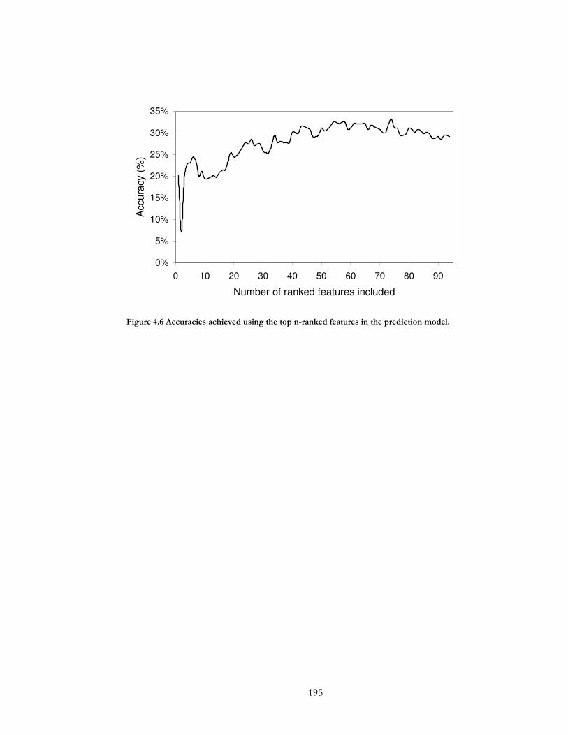
195

0%

5%

10%

15%

20%

25%

30%

35%

0 10 20 30 40 50 60 70 80 90

Number of ranked features included

Accu

racy (

%)

Figure 4.6 Accuracies achieved using the top n-ranked features in the prediction model.

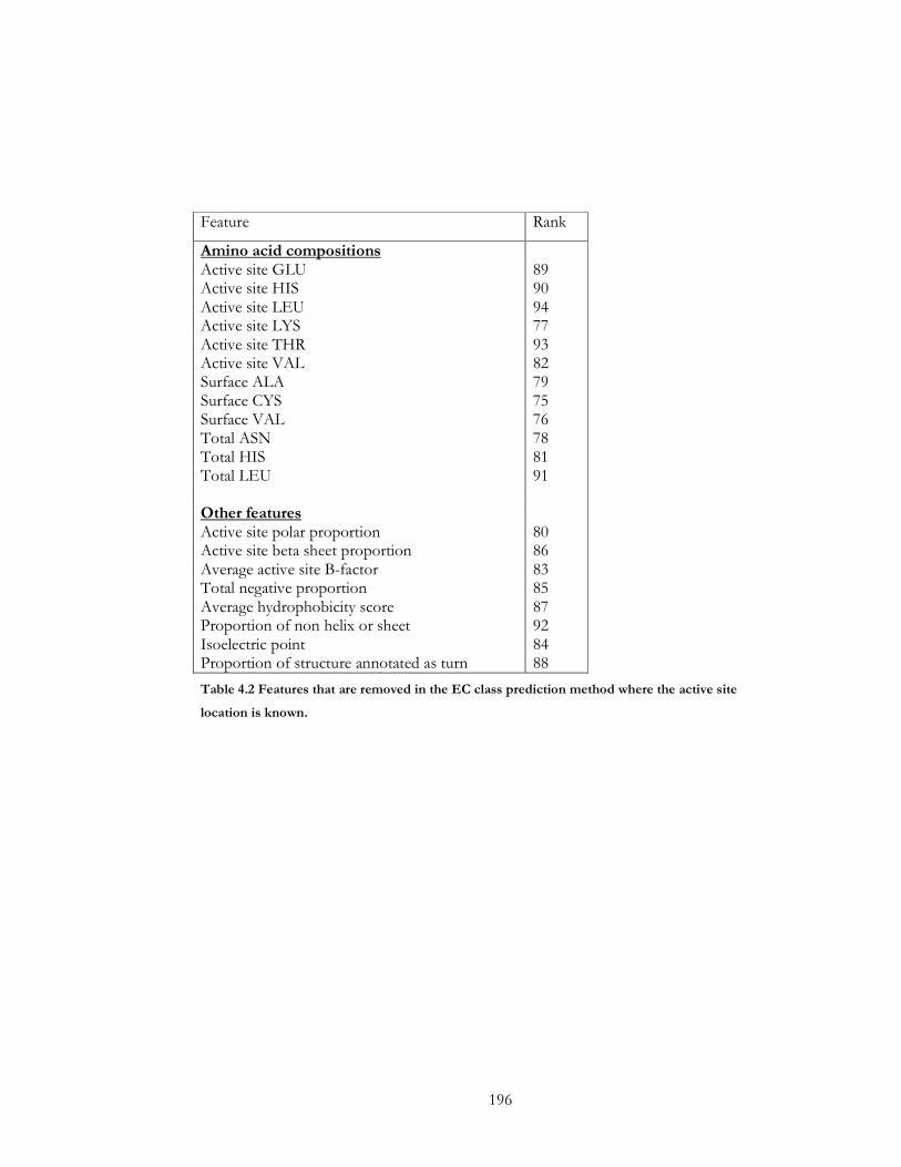
196

Feature Rank

Amino acid compositions Active site GLU 89 Active site HIS 90 Active site LEU 94 Active site LYS 77 Active site THR 93 Active site VAL 82 Surface ALA 79 Surface CYS 75 Surface VAL 76 Total ASN 78 Total HIS 81 Total LEU 91 Other features Active site polar proportion 80 Active site beta sheet proportion 86 Average active site B-factor 83 Total negative proportion 85 Average hydrophobicity score 87 Proportion of non helix or sheet 92 Isoelectric point 84 Proportion of structure annotated as turn 88 Table 4.2 Features that are removed in the EC class prediction method where the active site

location is known.

197

4.4 Predicting EC class for Enzymes with Predicted Active

Site Locations

The methodology for creating Dataset 4.2 described in 4.2.1 produced a dataset of 695

enzymes. Table 4.3 shows the number of enzymes in each EC class. This was split into

a training set of 625 structures and a test set of 70 structures. The distribution of

structures between the classes in the test set is representative of the class sizes in the

total dataset.

The best values for C and γ parameters were searched for by using the grid-searching

algorithm supplied in the LIBSVM package. Using parameters that were not weighted

by the class sizes, a maximum 10-fold cross-validation prediction accuracy of 38.2%

was achieved using 0.5 for both the C and the γ parameter. When class size

weightings were used (EC1 = 2.4, EC2= 1.3, EC3 = 1, EC4 = 2.8, EC5 = 3.9, EC6 =

5.5), the best prediction accuracy achieved was 36.0% (C = 8 and γ = 0.5) using a

coarse-grained grid search of the default range of C and γ parameter values (see Figure

4.7). A further grid search was then performed using a scale of 2-1 to 28 for C and 2-5 to

25 for γ. The optimal prediction accuracy remained at 36.0% with C = 8 and γ = 0.5.

EC class Number of enzyme structures

1 97 2 181 3 231 4 84 5 60 6 42

Table 4.3 The number of enzyme structures in each class in Dataset 4.2

198

Figure 4.7 Prediction accuracies achieved using a default grid search method for the best C and

γ parameters. A) Shows the accuracies on a 2D plot and B) shows this in 3D.

A

B

199

To reduce the effects of overfitting, features were removed that negatively contributed

to the model accuracy. The accuracies achieved using the top n-ranked features are

shown in Figure 4.8. The best prediction accuracy (39.0%) was achieved with the top

91 features. The final prediction model was then trained using a value of 8.0 for the C

and 0.5 the γ parameter and removing the 10 lowest ranked features (see Table 4.4)

from the training set.

32%

33%

34%

35%

36%

37%

38%

39%

40%

0 10 20 30 40 50 60 70 80 90 100

Feature rank

Accu

racy (

%)

Figure 4.8 Accuracies achieved using the top-ranked features with 10-fold cross-validation on

the training set.

The red line shows the minimum number of top-ranked features (91) needed to achieve the

maximum accuracy (39.0%).

Rank Feature 92 Total PRO

93 Proportion of active site B-sheet

94 Molecular weight

95 Surface PRO

96 Active site THR

97 Active site GLY

98 Active site ALA

99 Active site VAL

100 Presence of low complexity regions

101 Active site PRO

Table 4.4 The 10 lowest ranked features that were removed from the dataset to train the final

model.

200

The final prediction model using the optimized parameters and the 91 top-ranked

features was run on the testing dataset, which resulted in 32.9% accuracy (23 correct

class predictions out of 70). Despite the class weightings for the C parameter, the

larger classes had the best prediction accuracy. The best model achieved without class

weightings (the top-ranked 91 features and values of 0.5 for both parameters) resulted

in a higher accuracy of 34.3%. These predictions were, however, dominated by the

two largest classes (EC2 and EC3) and no cases were predicted as EC4, 5 or 6 and only

three cases were predicted as EC1 (see Table 4.5). Introducing weightings for the C

parameter reduced the overall accuracy achieved but the predictions it made were

slightly more balanced between the classes (see Figure 4.7).

Due to the lack of balance in the accuracy achieved between the classes, this method is

of limited use in real-world function prediction problems. Assuming that the accuracy

expected by random class choice is the sum of the squares of the class sizes divided by

the size of the dataset, the accuracy expected by random is 22.3%. Whilst the accuracy

achieved by this prediction method is 12% higher than this, it is still below that of the

percentage accuracy achieved by predicting all test cases as the largest class, EC3

(37%). Even predicting the second largest class, EC2, for all test cases would achieve a

prediction accuracy better than random selection (27%).

Actual EC Classification

Predicted EC Classification 1 2 3 4 5 6

Total (% correct)

1 2 0 1 0 0 0 3 (66.7%)

2 1 7 10 3 4 0 25 (28.0%)

3 6 12 15 6 2 1 42 (35.7%)

Total (% correct)

9 (22.2%)

19 (36.8%)

26 (57.7%)

9 (0%)

6 (0%)

1 (0%)

Table 4.5 The number of predictions of each class made by the model without class weightings.

The correct predictions are highlighted in green. No predictions were made by the model for

EC4-6.

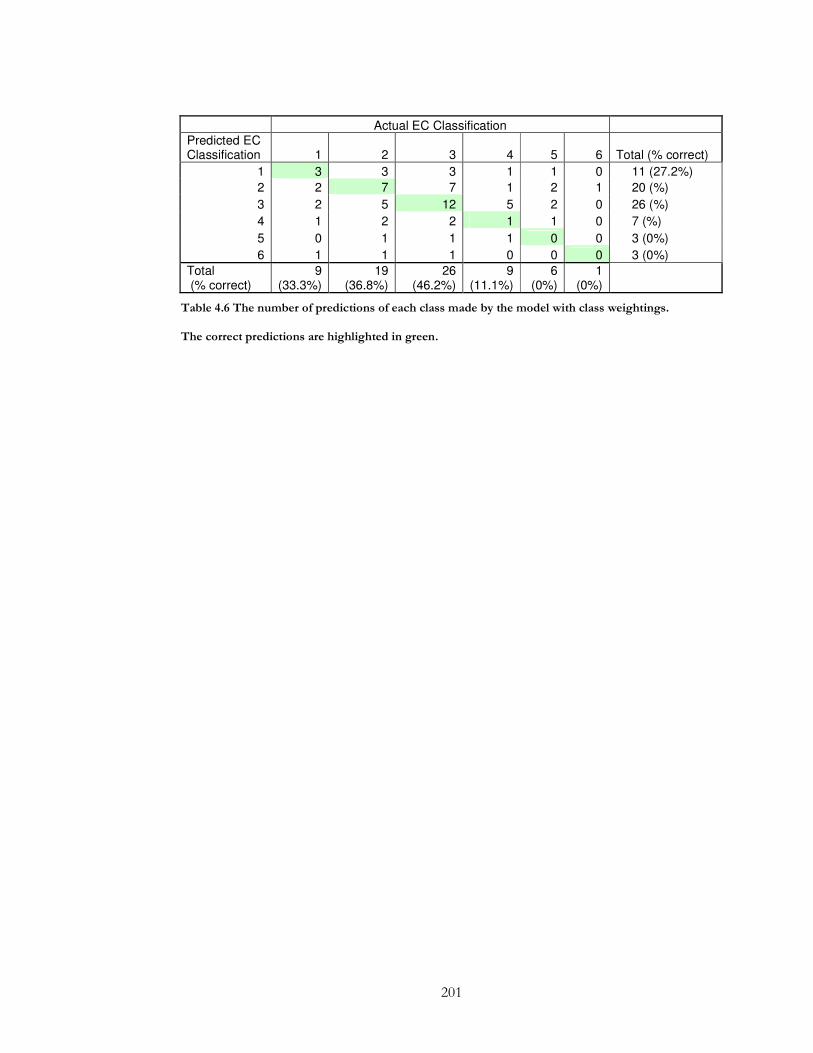
201

Actual EC Classification Predicted EC Classification 1 2 3 4 5 6 Total (% correct)

1 3 3 3 1 1 0 11 (27.2%)

2 2 7 7 1 2 1 20 (%)

3 2 5 12 5 2 0 26 (%)

4 1 2 2 1 1 0 7 (%)

5 0 1 1 1 0 0 3 (0%)

6 1 1 1 0 0 0 3 (0%)

Total (% correct)

9 (33.3%)

19 (36.8%)

26 (46.2%)

9 (11.1%)

6 (0%)

1 (0%)

Table 4.6 The number of predictions of each class made by the model with class weightings.

The correct predictions are highlighted in green.

202

4.5 Conclusions

The two prediction models presented in this chapter show that the information

contained in the features used in the model can be used to predict the top class of an

enzyme with better accuracy than random. The machine learning method, however, is

less able to deal with issues surrounding differing class sizes and results in imbalanced

prediction dominated by the largest classes.

The work in Chapter 2 attempts to deconstruct the relationships between differences in

features and the six functional classes on an individual basis. This showed trends in

individual features that were significantly different between the six EC classes for 20

features, of which three were explored further in relation to their functional

importance. The EC class prediction tools here attempt to quantify the usefulness of

these features in relation to predicting the top EC class of enzymes.

Of the 20 features that showed significant differences between EC classes listed in

Chapter 2, 6 of them were not used in the prediction model using known active sites

(prediction model 1) and one feature was not used in the machine learning method

(prediction model 2).

The active site aromatic proportion and the active site phenylalanine proportion were

not included in prediction model 1, but both strongly correlate with the active site

tryptophan proportion (from Chapter 2), which was included. Similarly, the active site

non-polar proportion was not included in prediction model 1 whilst active site

hydrophobicity, which correlated strongly with the active site non-polar proportion

(from Chapter 2), was included. The other three significant features not included in

prediction model 1, relative active site surface area, sequence length (which both

strongly correlated with each other) and total isoleucine proportion, were not strongly

correlated with other features that were included in the model. Only one of the

significantly different features (total proline composition) from the analysis in Chapter

2 was not used in the machine learning method (prediction model 2).

203

4.6 References

1. Bray T, Doig AJ, Warwicker J. Sequence and structural features of enzymes and their active sites by EC class. J Mol Biol 2009;386(5):1423-1436.

2. Berman HM, Westbrook J, Feng Z, Gilliland G, Bhat TN, Weissig H, Shindyalov IN, Bourne PE. The Protein Data Bank. Nucleic Acids Res 2000;28(1):235-242.

3. Friedberg I, Jambon M, Godzik A. New avenues in protein function prediction. Protein Sci 2006;15(6):1527-1529.

4. Doppelt O, Moriaud F, Bornot A, de Brevern AG. Functional annotation strategy for protein structures. Bioinformation 2007;1(9):357-359.

5. Lin HH, Han LY, Zhang HL, Zheng CJ, Xie B, Cao ZW, Chen YZ. Prediction of the functional class of metal-binding proteins from sequence derived physicochemical properties by support vector machine approach. BMC Bioinformatics 2006;7 Suppl 5:S13.

6. Lin HH, Han LY, Zhang HL, Zheng CJ, Xie B, Chen YZ. Prediction of the functional class of lipid binding proteins from sequence-derived properties irrespective of sequence similarity. J Lipid Res 2006;47(4):824-831.

7. Han LY, Cai CZ, Lo SL, Chung MC, Chen YZ. Prediction of RNA-binding proteins from primary sequence by a support vector machine approach. Rna 2004;10(3):355-368.

8. Cai CZ, Han LY, Ji ZL, Chen YZ. Enzyme family classification by support vector machines. Proteins 2004;55(1):66-76.

9. Cai CZ, Han LY, Ji ZL, Chen X, Chen YZ. SVM-Prot: Web-based support vector machine software for functional classification of a protein from its primary sequence. Nucleic Acids Res 2003;31(13):3692-3697.

10. Stawiski EW, Baucom AE, Lohr SC, Gregoret LM. Predicting protein function from structure: unique structural features of proteases. Proc Natl Acad Sci U S A 2000;97(8):3954-3958.

11. Stawiski EW, Mandel-Gutfreund Y, Lowenthal AC, Gregoret LM. Progress in predicting protein function from structure: unique features of O-glycosidases. Pac Symp Biocomput 2002:637-648.

12. Dobson PD, Doig AJ. Predicting enzyme class from protein structure without alignments. J Mol Biol 2005;345(1):187-199.

13. Dobson PD, Doig AJ. Distinguishing enzyme structures from non-enzymes without alignments. J Mol Biol 2003;330(4):771-783.

14. Chandonia JM, Hon G, Walker NS, Lo Conte L, Koehl P, Levitt M, Brenner SE. The ASTRAL Compendium in 2004. Nucleic Acids Res 2004;32(Database issue):D189-192.

15. Murzin AG, Brenner SE, Hubbard T, Chothia C. SCOP: a structural classification of proteins database for the investigation of sequences and structures. J Mol Biol 1995;247(4):536-540.

16. Porter CT, Bartlett GJ, Thornton JM. The Catalytic Site Atlas: a resource of catalytic sites and residues identified in enzymes using structural data. Nucleic Acids Res 2004;32(Database issue):D129-133.

17. Apweiler R MM, O'Donovan C, Magrane M, Alam-Faruque Y, Antunes R, Barrell D, Bely B, Bingley M, Binns D, Bower L, Browne P, Chan WM, Dimmer E, Eberhardt R, Fedotov A, Foulger R, Garavelli J, Huntley R, Jacobsen J, Kleen M, Laiho K, Leinonen R, Legge D, Lin Q, Liu W, Luo J, Orchard S, Patient S, Poggioli D, Pruess M, Corbett M, di Martino G, Donnelly

204

M, van Rensburg P, Bairoch A, Bougueleret L, Xenarios I, Altairac S, Auchincloss A, Argoud-Puy G, Axelsen K, Baratin D, Blatter MC, Boeckmann B, Bolleman J, Bollondi L, Boutet E, Quintaje SB, Breuza L, Bridge A, deCastro E, Ciapina L, Coral D, Coudert E, Cusin I, Delbard G, Doche M, Dornevil D, Roggli PD, Duvaud S, Estreicher A, Famiglietti L, Feuermann M, Gehant S, Farriol-Mathis N, Ferro S, Gasteiger E, Gateau A, Gerritsen V, Gos A, Gruaz-Gumowski N, Hinz U, Hulo C, Hulo N, James J, Jimenez S, Jungo F, Kappler T, Keller G, Lachaize C, Lane-Guermonprez L, Langendijk-Genevaux P, Lara V, Lemercier P, Lieberherr D, de Oliveira Lima T, Mangold V, Martin X, Masson P, Moinat M, Morgat A, Mottaz A, Paesano S, Pedruzzi I, Pilbout S, Pillet V, Poux S, Pozzato M, Redaschi N, Rivoire C, Roechert B, Schneider M, Sigrist C, Sonesson K, Staehli S, Stanley E, Stutz A, Sundaram S, Tognolli M, Verbregue L, Veuthey AL, Yip L, Zuletta L, Wu C, Arighi C, Arminski L, Barker W, Chen C, Chen Y, Hu ZZ, Huang H, Mazumder R, McGarvey P, Natale DA, Nchoutmboube J, Petrova N, Subramanian N, Suzek BE, Ugochukwu U, Vasudevan S, Vinayaka CR, Yeh LS, Zhang J. The Universal Protein Resource (UniProt) in 2010. Nucleic Acids Res 2010;38(Database issue):D142-148.

18. Kabsch W, Sander C. Dictionary of protein secondary structure: pattern recognition of hydrogen-bonded and geometrical features. Biopolymers 1983;22(12):2577-2637.

19. Hutchinson EG, Thornton JM. PROMOTIF--a program to identify and analyze structural motifs in proteins. Protein Sci 1996;5(2):212-220.

20. Rice P, Longden I, Bleasby A. EMBOSS: the European Molecular Biology Open Software Suite. Trends Genet 2000;16(6):276-277.

21. Kyte J, Doolittle RF. A simple method for displaying the hydropathic character of a protein. J Mol Biol 1982;157(1):105-132.

22. Wootton JC, Federhen S. Analysis of compositionally biased regions in sequence databases. Methods Enzymol 1996;266:554-571.

23. Chih-Chung Chang C-JL. LIBSVM : a library for support vector machines. Software available at http://wwwcsientuedutw/~cjlin/libsvm 2001.

205

Chapter 5: Gaussian Network Modeling of

Oligomeric Proteins

One of the observations resulting from an analysis of differences in structural and

sequence features between EC classes in Chapter 2 was that lyases (EC4) tend to prefer

to exist as oligomers and conversely hydrolases (EC3) preferred to exist as monomers.

The preference for different oligomeric statuses in these functions was linked to the

function’s over/under-representation at highly loaded points in metabolic networks. It

was suggested that some metabolically important enzymes may have evolved to exist as

oligomers in order to enable them to be regulated via mechanisms such as

cooperativity.

Due to the difficulty in obtaining biochemical data for a large amount of structures in

order to further investigate this theory, a method to detect cooperative action from

enzyme structure was required. Currently no such computational method exists for

this purpose and this chapter begins with an attempt to address this. It goes on to

further investigate the patterns of coupled motions in protein structures in terms of

enzyme active sites and as a feature of oligomeric structures in general.

5.1 Introduction

5.1.1 Cooperativity in Oligomeric Enzymes

Cooperativity, in relation to oligomeric enzymes, describes enzymes where the affinity

of binding of a ligand at one binding site induces a change in the rate of binding of the

ligand at further sites on the enzyme. Bohr et al. first noticed that the oxygen binding

curve for hemoglobin was sigmoidal and suggested that the binding of the first oxygen

molecule made it easier for subsequent oxygen molecules to bind1.

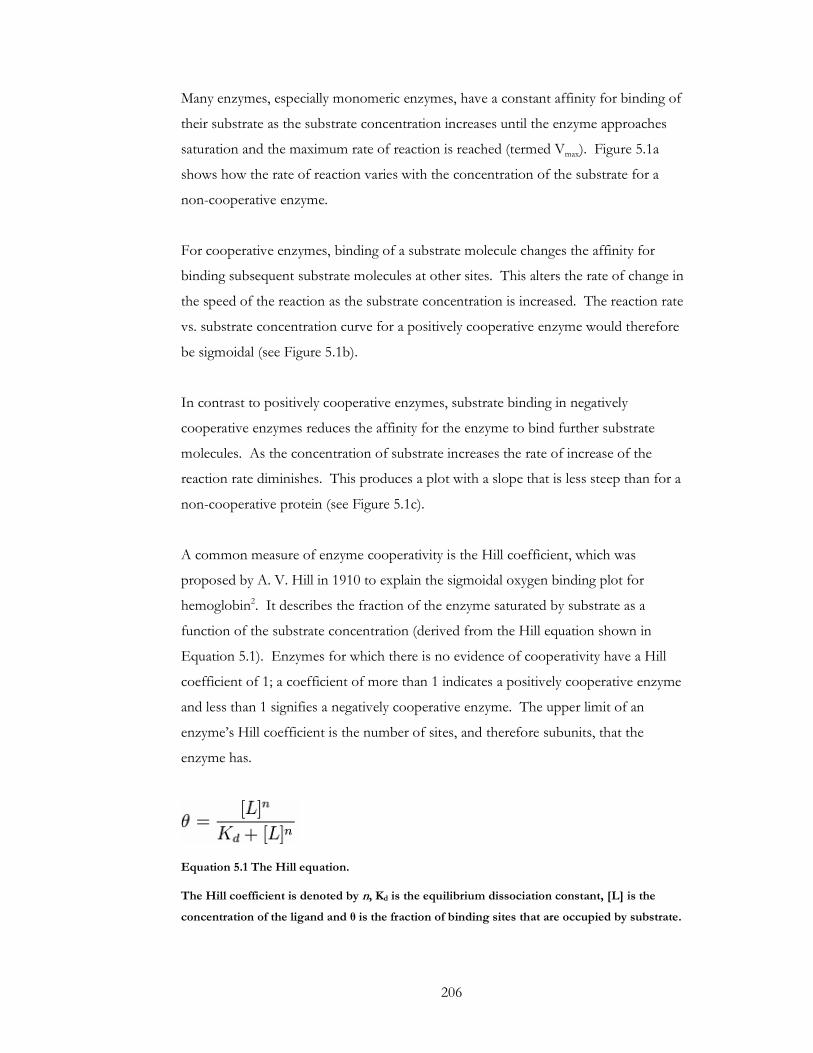
206

Many enzymes, especially monomeric enzymes, have a constant affinity for binding of

their substrate as the substrate concentration increases until the enzyme approaches

saturation and the maximum rate of reaction is reached (termed Vmax). Figure 5.1a

shows how the rate of reaction varies with the concentration of the substrate for a

non-cooperative enzyme.

For cooperative enzymes, binding of a substrate molecule changes the affinity for

binding subsequent substrate molecules at other sites. This alters the rate of change in

the speed of the reaction as the substrate concentration is increased. The reaction rate

vs. substrate concentration curve for a positively cooperative enzyme would therefore

be sigmoidal (see Figure 5.1b).

In contrast to positively cooperative enzymes, substrate binding in negatively

cooperative enzymes reduces the affinity for the enzyme to bind further substrate

molecules. As the concentration of substrate increases the rate of increase of the

reaction rate diminishes. This produces a plot with a slope that is less steep than for a

non-cooperative protein (see Figure 5.1c).

A common measure of enzyme cooperativity is the Hill coefficient, which was

proposed by A. V. Hill in 1910 to explain the sigmoidal oxygen binding plot for

hemoglobin2. It describes the fraction of the enzyme saturated by substrate as a

function of the substrate concentration (derived from the Hill equation shown in

Equation 5.1). Enzymes for which there is no evidence of cooperativity have a Hill

coefficient of 1; a coefficient of more than 1 indicates a positively cooperative enzyme

and less than 1 signifies a negatively cooperative enzyme. The upper limit of an

enzyme’s Hill coefficient is the number of sites, and therefore subunits, that the

enzyme has.

Equation 5.1 The Hill equation.

The Hill coefficient is denoted by n, Kd is the equilibrium dissociation constant, [L] is the

concentration of the ligand and θ is the fraction of binding sites that are occupied by substrate.

207

A

B

C

Figure 5.1 Example reaction rate (v/Vmax) vs.

substrate concentration ([S]) for a non-

cooperative (A), a positively cooperative (B)

and a negatively cooperate enzyme (C).

The grey line in figure shows the curve expected

from a non-cooperative enzymes in comparison

to the negative cooperative black line.

208

The response coefficient, RS, was proposed by Koshland et al. as a measure of an

enzyme’s sensitivity3. It measures the difference between the concentrations of

substrate required at 10% and 90% of the maximum reaction rate. For enzymes that

follow Michaelis-Menten kinetics the response coefficient RS equals 81, but for

positively cooperative enzymes the change in substrate required to increase the reaction

rate from 10% to 90% of Vmax is much less. An enzyme with a hill coefficient of 2.5,

for example, has a response coefficient of only 5. This allows the enzyme to react with

greater sensitivity to small changes in substrate concentrations.

Sensitivity to changes in substrate concentrations is important in many key biological

processes and can act as a further control mechanism for biochemically important

enzymes, particularly where substrate concentrations are low. For example, in cases

where defective hemoglobin lacks the ability to bind oxygen cooperatively in humans,

it causes cyanosis (a blue pigmentation of the skin due to oxygen saturation typically

dropping below 85%), which can have devastating effects4. Cooperativity can be used

as a mechanism to change the reaction kinetics of an enzyme without changing the

critical arrangement of the enzyme active site5. The arrangement of the oxygen-

binding site in hemoglobin is critical to its function and is highly conserved over

different organisms. Changes in environmental constraints for an organism (for

example between the amphibious environment of the frog and the aqueous

environment of the tadpole) dictate different binding kinetics, which can be altered by

varying the subunit interactions without disturbing the critical binding-site residues6.

As the response to substrate concentration is damped for negatively cooperative

enzymes the change in substrate concentration required to increase the reaction rate

from 10% to 90% of Vmax is often significantly larger than a non-cooperative enzyme.

This effectively increases the range of substrate concentrations over which the enzyme

is active. This is particularly advantageous to enzymes for which it is critical to

maintain some level of reaction in stressful situations where usually-plentiful

metabolites are in short supply5. There is also a suggestion that branch-point enzymes

are likely to act cooperatively in order to ensure that the multiple pathways that rely on

the products of that branch point enzyme are not inhibited by an excess of one

substrate5.

209

A further level of control for cooperative enzymes may exist due to their oligomeric

status. Errors in transcription or translation rarely have a dramatic effect on an

enzyme’s activity unless the mutation occurs at the enzyme’s binding site. A single

residue mutation may have little or no effect on a non-cooperative, monomeric enzyme

outside of these functionally critical areas. Even in a non-cooperative oligomer,

without the need for interaction between cooperatively-acting subunits, a mutation that

disturbs the oligomeric interfaces may have little phenotypic effect. As mentioned

above for hemoglobin, mutations that affect the subunit interface and therefore the

ability to act cooperatively can have damaging effects on the rate of binding. A larger

proportion of a cooperative enzyme’s residues is therefore functionally constrained

than for a non-cooperative enzyme and provides further support for cooperativity as a

mechanism for tight catalytic control in metabolic systems.

Unfortunately the amount and quality of cooperativity data for enzymes is patchy and

inconsistent. To evaluate the extent of cooperativity as a metabolic control mechanism

in tightly regulated enzymes it is necessary to be able to identify enzymes that are (or

are not) cooperative without lengthy and detailed biochemical experiment on individual

enzymes. Currently there is no computational approach to distinguish oligomeric

enzymes that are likely to act cooperatively and those that are not. As outlined below,

computational analyses of structural dynamics on an individual basis have been able to

characterise allosteric mechanisms and here it is assessed whether general dynamic

properties, such as the degree of correlation of motion over oligomer subunits, are

indicative of enzyme cooperativity. In particular, it is questioned whether the

communication between active sites on cooperative proteins is mediated or observable

through coupled motion in dynamic fluctuations between residues.

210

5.1.2 Application of Normal Mode Analysis to the Study of Proteins

It is well documented that a protein’s function is not entirely coded in its DNA or

protein sequence7; 8; 9; 10 and despite the increasing availability of protein structures

thanks to structural genomics initiatives, the gap between sequence and function

cannot yet be accounted for by structure alone. Since biological activity in proteins is

often accompanied with a change in protein structural conformation, perhaps these

conformational changes contain further functional information that is missing from the

sequence and structure alone. The study of protein dynamics has become increasingly

popular over the last 20 years and has growing recognition as an important additional

step in the sequence, structure and function paradigm.

Despite computing power having increased dramatically since the first protein

structures were produced, modeling these conformational changes over relevant

timescales is still difficult due to the total number of conformations available to a

protein in solution. Functional proteins in native state conditions however, tend to

sample conformations in equilibrium around their folded state. These subsets of

available conformations are termed microstates and modeling their vibrational modes is

a fast and efficient way of approximating them. Approaches such as Normal Mode

Analysis (NMA) have been used to successfully model proteins dynamics for over 25

years11 and have become even more popular as computational capacity increases.

This increase in popularity has prompted a number of simple models based on NMA

to assess large-scale protein dynamics quickly and efficiently12; 13; 14; 15; 16. These methods

are particularly useful in modeling dynamics in large systems, for which more detailed

methods such as molecular dynamics are too computationally expensive to be feasible.

Despite the coarse-grained nature of these methods, they have been found to give

remarkably similar results to complex methods such as molecular dynamics12; 17; 18. It is

also surprising that the resolution of the model has little effect on the results of

modeling dynamic motion of a protein in this way, indeed it has been shown that

motion can be modeled sufficiently accurately in the absence of crystal structure

coordinates by using electron density maps obtained from cryo-electon microscopy or

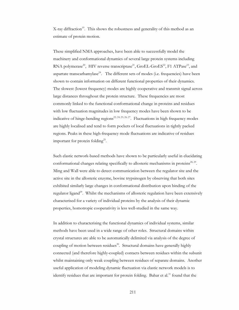
211

X-ray diffraction19. This shows the robustness and generality of this method as an

estimate of protein motion.

These simplified NMA approaches, have been able to successfully model the

machinery and conformational dynamics of several large protein systems including

RNA polymerase20, HIV reverse transcriptase21, GroEL-GroES22, F1 ATPase23, and

aspartate transcarbamylase24. The different sets of modes (i.e. frequencies) have been

shown to contain information on different functional properties of their dynamics.

The slowest (lowest frequency) modes are highly cooperative and transmit signal across

large distances throughout the protein structure. These frequencies are most

commonly linked to the functional conformational change in proteins and residues

with low fluctuation magnitudes in low frequency modes have been shown to be

indicative of hinge-bending regions22; 24; 25; 26; 27. Fluctuations in high frequency modes

are highly localised and tend to form pockets of local fluctuations in tightly packed

regions. Peaks in these high-frequency mode fluctuations are indicative of residues

important for protein folding25.

Such elastic network-based methods have shown to be particularly useful in elucidating

conformational changes relating specifically to allosteric mechanisms in proteins28; 29.

Ming and Wall were able to detect communication between the regulator site and the

active site in the allosteric enzyme, bovine trypsinogen by observing that both sites

exhibited similarly large changes in conformational distribution upon binding of the

regulator ligand29. Whilst the mechanisms of allosteric regulation have been extensively

characterised for a variety of individual proteins by the analysis of their dynamic

properties, homotropic cooperativity is less well-studied in the same way.

In addition to characterising the functional dynamics of individual systems, similar

methods have been used in a wide range of other roles. Structural domains within

crystal structures are able to be automatically delimited via analysis of the degree of

coupling of motion between residues30. Structural domains have generally highly

connected (and therefore highly-coupled) contacts between residues within the subunit

whilst maintaining only weak coupling between residues of separate domains. Another

useful application of modeling dynamic fluctuation via elastic network models is to

identify residues that are important for protein folding. Bahar et al.31 found that the

212

magnitude of fluctuations correlated with the resistance of residues to undergo

hydrogen-deuterium exchange and it was suggested that the more protected residues

are more critical to the folding process. Similar studies have also found that residues

with peak fluctuation displacements in the fast modes are critical to folding32 and have

gone on to specifically predict folding cores17.

The simplicity, robustness and speed of these models make them attractive to large-

scale analysis of protein dynamics and their success in elucidating functional

conformational change in proteins makes them an attractive choice for this analysis.

Amongst the simplified models based on NMA, the Gaussian Network Model (GNM),

described in further detail in 5.1.3, is one of the most commonly used and has been

shown to give good correlation between theoretical and experimental data33. Many

software applications and webservers are available to model the dynamics of a given

protein structure34; 35; 36 and thus it is not necessary to create a new method as part of

this work.

Since it has been shown that conformational change on binding correlates with

dynamic motion intrinsic in the native folded protein37, and it has been suggested that

communication can be transmitted between distant sites without large-scale

conformational changes38, it was hypothesised that cooperativity can be detected from

dynamic fluctuations in a protein’s native folded structure. It is reasonable to imagine

that the cooperative action between multiple active sites on separate subunits may be

communicated via dynamic motion intrinsic in the structure and that it may result in

correlated fluctuations between the active site residues.

213

5.1.3 Normal Mode Analysis and the Gaussian Network Model

A protein can be imagined as a system of oscillating nodes, the normal modes of which

are the patterns of motion where all parts move sinusoidally. This can occur at

different frequencies for different systems and such frequencies are called natural

frequencies. Normal Mode Analysis (NMA) assumes that near the energy minimum of

a system, forces act like springs, which can be approximated by atomic force-fields

taken from molecular dynamics simulations. One of the major computational hurdles

of NMA is minimizing the energy of the system before the normal modes can be

analysed. The computational overhead of this step has led to the application of NMA

to more simplified models, such as the elastic network model.

One such application of this approach is Gaussian Network Modeling (GNM)12. It is

based on the above principles but rather than having to minimize the energy of a

system, the normal modes are evaluated on a simple elastic network of nodes that

represent the protein structure (see Figure 5.2). Each residue is represented by a node,

which corresponds to its alpha carbon coordinates and a network topology is built by

connecting nodes within a given cutoff distance. An all-atom model can also be

constructed by representing each atom with a node, but this increases the

computational overhead beyond any advantage that the increased resolution provides.

Indeed, it has been shown that coarse-grained models give comparably representative

results to all-atom models39.

The connections between nodes in this elastic network are modeled as springs,

enabling the nodes to move with Gaussian motion around their coordinates with

varying frequencies according to each mode. In GNM the fluctuations are assumed to

be isotropic, which means that the fluctuation is uniform in all directions. This is

where GNM differs to NMA applied to elastic networks (also termed Anisotropic

Network Modeling [ANM]) as the latter do not assume fluctuations are isotropic. In

the context of this analysis the degree of similarity in fluctuations between residues is

important rather than the overall direction of the movement and therefore GNM is

214

preferred for this analysis. GNM results have also been shown to give higher

agreement to experimental B-factors than ANM33.

Figure 5.2 A protein structure (lysine–arginine–ornithine binding protein; top) shown as an

elastic network.

The nodes represent residues and the lines represent the elastic connections between them.

Picture taken from Tama and Sanejouand, 2001.15

215

Of interest in this analysis is the degree of similarity between the fluctuations of pairs

of residues. In GNM this information is derived in the following way:

• If the equilibrium position vectors of a residue i as Ri0 and the position of the

node in this vector at any one time as Ri, the fluctuations around the starting

point can be described as ∆Ri = Ri – Ri0

• The fluctuations of the other residue, j, in the pair are defined as above (∆Rj).

• The difference vector between these two residue fluctuations is described as

∆Rij = ∆Ri – ∆Rj (see Figure 5.3 for a schematic representation).

• The correlation of fluctuations for i and j is given by the dot product of their

fluctuation vectors (see Equation 5.2) using the statistical mechanical

probabilities defined by the GNM method12. The overall correlation between

the two residues is obtained by summing over all non-zero modes.

There are many webservers and software applications that can perform normal mode

analysis for a given protein, but most deliver the anisotropic NMA/elastic network

method35; 36. As mentioned above, the isotropic GNM approach was deemed more

suitable for this analysis. The Bahar group have produced a webserver, oGNM34, that

performs GNM analysis of a given protein structure. In addition to mode shapes and

mean square fluctuations (displacements), it also provides a cross-correlation matrix for

all residues versus all residues, which forms the basis of the data used in this chapter.

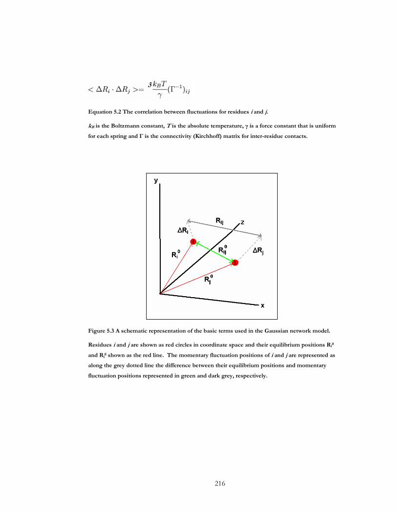
216

Equation 5.2 The correlation between fluctuations for residues i and j.

kB is the Boltzmann constant, T is the absolute temperature, γ is a force constant that is uniform

for each spring and Г is the connectivity (Kirchhoff) matrix for inter-residue contacts.

Figure 5.3 A schematic representation of the basic terms used in the Gaussian network model.

Residues i and j are shown as red circles in coordinate space and their equilibrium positions Ri0

and Rj0 shown as the red line. The momentary fluctuation positions of i and j are represented as

along the grey dotted line the difference between their equilibrium positions and momentary

fluctuation positions represented in green and dark grey, respectively.

217

5.2 Methods

5.2.1 Dataset Creation for the Cooperativity Analysis

To test the hypothesis that the active sites of cooperative enzymes exhibit increased

correlation of motion over non-site residues than non-cooperative enzymes it was

necessary to collect a collection of structures of known cooperative enzymes. There is

currently no database that holds large-scale information about cooperative enzymes.

Enzyme databases such as BRENDA40 and SABIO-RK41 annotate entries with their

hill coefficients where this is available but the number of enzymes with this

information given is relatively small.

It is further necessary for enzymes with known hill coefficient data to have a known

structure deposited in the PDB. It is also important to ensure that the enzyme

structure is from the same organism as the hill coefficient is reported for as it has been

shown that cooperativity can vary for the same protein between different organisms42.

A review by Koshland and Hamadani5 attempted to estimate the comparative

proportions of negatively cooperative and positively cooperative enzymes in nature by

surveying the literature from 1980-1990. In doing so they produced small datasets of

positive, negative and non-cooperative enzymes. Many of these enzymes, however,

could not be associated with a PDB structure from the same organism. A benchmark

set of allosteric protein structures was reported by Daily and Gray43, however allosteric

proteins are not necessarily cooperative and only a subset of the enzymes they list are

cooperative.

The most productive source of cooperative enzyme information was the database,

SABIO RK41. This is a database containing information about biochemical reactions,

alongside their kinetic equations and associated parameters. The reaction pathways and

enzyme annotation in SABIO RK is obtained from KEGG44 and reaction kinetics are

annotated by manual literature curation. This focus on reaction kinetics using literature

218

curation results in a larger number of entries for which there is Hill coefficient

information than BRENDA or KEGG.

In addition to the above data sources, a literature search was performed in order to

find papers for individual enzymes that report the hill coefficients of ligand binding.

Since a null set (i.e. non-cooperative proteins) was needed, enzymes were also recorded

where a hill coefficient of 1 was reported, in addition to negatively and positively

cooperative enzymes. Enzymes were matched to PDB structures via their Uniprot

entry and where more than one PDB structure exists for the enzyme, preference was

given to the highest resolution structure where the ligand that the hill coefficient relates

to is present. Table 5.1 shows the resultant dataset (named Dataset 5.1) that was

obtained from these sources.

This analysis also required the location of the active site to be known for each of the

proteins in the set. Since each of these proteins has been relatively well-studied in

order to report detailed biochemical parameters, the active sites for each of the

proteins is very likely to already be known. If the PDB file contained the enzyme’s

ligand then active site residues were defined as those that had any atom within 3Å of

the bound ligand. If the PDB structure did not contain a bound ligand, either the

residues listed in the SITE records in the PDB file (if present) or in that structure’s

entry in the CSA were used.

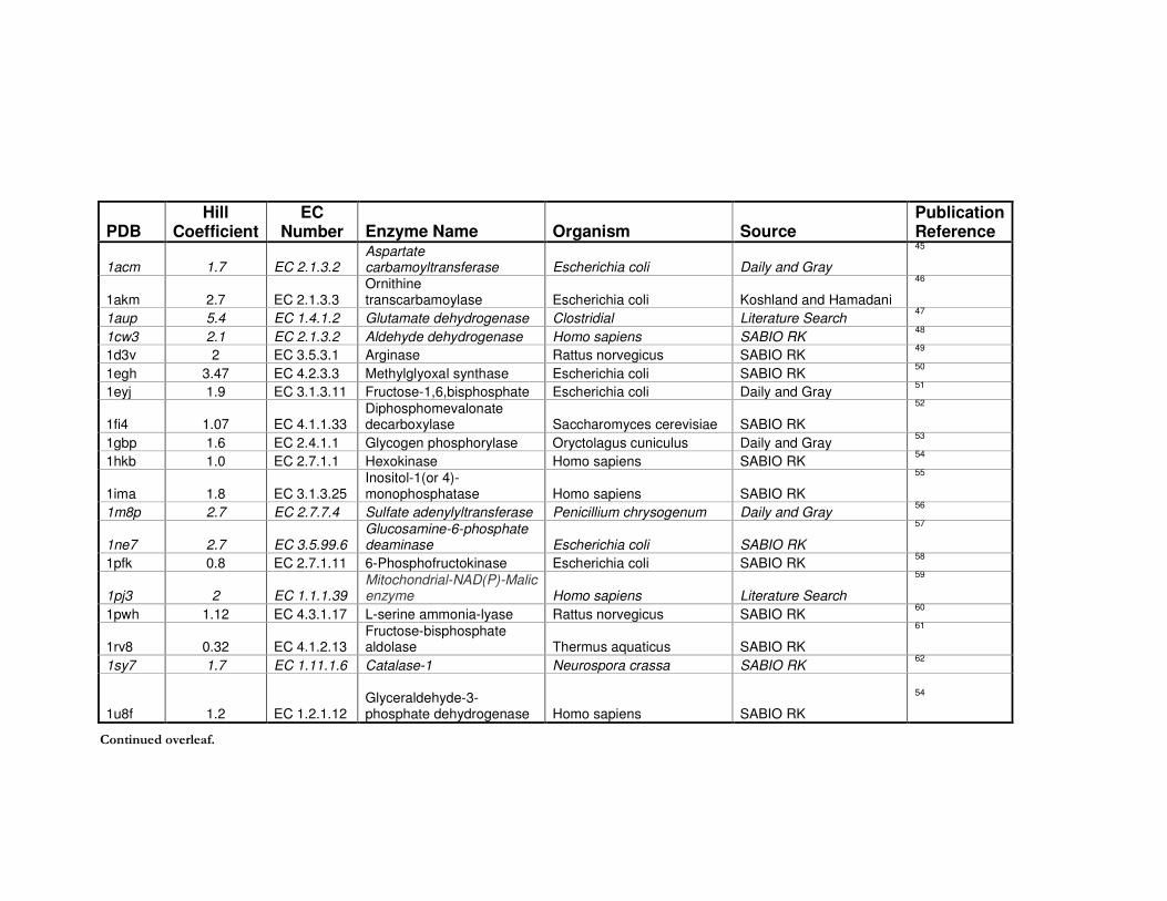
PDB Hill

Coefficient EC

Number Enzyme Name Organism Source Publication Reference

1acm 1.7 EC 2.1.3.2 Aspartate carbamoyltransferase Escherichia coli Daily and Gray

45

1akm 2.7 EC 2.1.3.3 Ornithine transcarbamoylase Escherichia coli Koshland and Hamadani

46

1aup 5.4 EC 1.4.1.2 Glutamate dehydrogenase Clostridial Literature Search 47

1cw3 2.1 EC 2.1.3.2 Aldehyde dehydrogenase Homo sapiens SABIO RK 48

1d3v 2 EC 3.5.3.1 Arginase Rattus norvegicus SABIO RK 49

1egh 3.47 EC 4.2.3.3 Methylglyoxal synthase Escherichia coli SABIO RK 50

1eyj 1.9 EC 3.1.3.11 Fructose-1,6,bisphosphate Escherichia coli Daily and Gray 51

1fi4 1.07 EC 4.1.1.33 Diphosphomevalonate decarboxylase Saccharomyces cerevisiae SABIO RK

52

1gbp 1.6 EC 2.4.1.1 Glycogen phosphorylase Oryctolagus cuniculus Daily and Gray 53

1hkb 1.0 EC 2.7.1.1 Hexokinase Homo sapiens SABIO RK 54

1ima 1.8 EC 3.1.3.25 Inositol-1(or 4)-monophosphatase Homo sapiens SABIO RK

55

1m8p 2.7 EC 2.7.7.4 Sulfate adenylyltransferase Penicillium chrysogenum Daily and Gray 56

1ne7 2.7 EC 3.5.99.6 Glucosamine-6-phosphate deaminase Escherichia coli SABIO RK

57

1pfk 0.8 EC 2.7.1.11 6-Phosphofructokinase Escherichia coli SABIO RK 58

1pj3 2 EC 1.1.1.39 Mitochondrial-NAD(P)-Malic enzyme Homo sapiens Literature Search

59

1pwh 1.12 EC 4.3.1.17 L-serine ammonia-lyase Rattus norvegicus SABIO RK 60

1rv8 0.32 EC 4.1.2.13 Fructose-bisphosphate aldolase Thermus aquaticus SABIO RK

61

1sy7 1.7 EC 1.11.1.6 Catalase-1 Neurospora crassa SABIO RK 62

1u8f 1.2 EC 1.2.1.12 Glyceraldehyde-3-phosphate dehydrogenase Homo sapiens SABIO RK

54

Continued overleaf.

220

PDB

Hill Coefficient EC Number Enzyme Name Organism Source

Publication Reference

1vgv 1.8 EC 5.3.1.14 UDP-N-acetylglucosamine 2-epimerase Escherichia coli SABIO RK

63

1xbt 0.8 EC 2.7.1.21 Thymidine kinase Homo sapiens SABIO RK 64

1xge 1.57 EC 3.5.2.3 Dihydroorotase Escherichia coli Literature Search 65

1xva 2.3 EC 2.2.1.20 Glycine Methyltransferase Rattus norvegicus Koshland and Hamadani 66

1xz8 1.0 EC 2.4.2.9 uracil phosphoribosyltransferase Bacillus caldolyticus Daily and Gray

67

1y3i 1.4 EC 2.7.1.23 NAD+ kinase Mycobacterium tuberculosis BRENDA 68

2bz0 1.3 EC 3.5.4.25 GTP cyclohydrolase II Escherichia coli BRENDA 69

2csm 1.6 EC 5.4.99.5 Chorismate mutase Saccharomyces cerevisiae Daily and Gray 70

2hbq 1.5 EC 3.4.2.36 Caspase I Homo sapiens Daily and Gray 71

2hgs 0.8 EC 6.3.2.3 Glutathione synthase Homo sapiens SABIO RK 72

2hxd 1.9 EC 3.5.4.30 dCTP deaminase Methanococcus jannaschii SABIO RK 73

2jlc 1.0 EC 2.5.1.64

2-Succinyl-6-hydroxy-2,4-cyclohexadiene-1-carboxylate Escherichia coli SABIO RK

74

2pah 1.6 EC 1.14.16.1 Phenylalanine 4-monooxygenase Homo sapiens SABIO RK

75

Table 5.1 Dataset 5.1: A list of enzymes with annotated Hill coefficients and a structure deposited in the PDB for the same organism.

Enzymes shown in italics are later deleted from the dataset for technical reasons.

5.2.2 Dataset Creation for the Active Site Correlation Analysis

In order to test the hypothesis that active site residues are generally more coupled than

non-active site residues, a test set of homo-oligomeric enzymes with known structures

and annotated active sites was needed. The non-redundant set of enzymes with

literature active site annotation from the Catalytic Sites Atlas (CSA)76 that was used to

test active site predictions in Chapter 5: was used again here (details of creation of this

dataset are given in 3.2.2). Only the structures that contained 2 or more identical

chains were applicable to this analysis and those proteins with more than 9 chains were

discarded due to the technical reasons discussed in 5.2.4.

The resultant dataset (Dataset 5.2, shown in Table 5.2) contains 114 non redundant

homo-oligomeric enzyme structures with a literature-annotated active site. The active

site residues for these proteins were defined in the same way as described in 2.2.2.

1a4i 1n20 1f75 1e2a 1d2t

1b5t 1nir 1f7l 1f8x 1dco

1c9u 1nww 1fua 1fro 1dxe

1cd5 1qrg 1gpj 1hrk 1ez2

1cgk 1r16 1gpr 1jfl 1j80

1cs1 1r51 1j7g 1nn5 1jm7

1d8h 1wgi 1kp2 1oe9 1m6k

1dhf 1yve 1mka 1otg 1moq

1dqa 12as 1nid 1qh6 1mvn

1e7l 1a05 1nsp 1qpr 1nf10

1ecm 1a79 1snn 1qq6 1o9i

1ef0 1a95 1sox 1r4f 1oac

1g79 1b65 1tys 1r6w 1oas

1gqg 1b93 1uro 1uf8 1pfk

1hxq 1brw 3cla 2jcw 1qj5

1i6p 1cg6 3eca 2toh 1rhc

1ir3 1d4a 3mdd 7odc 1ro8

1jdw 1daa 1c2t 1al7 1tph

1jhf 1dci 1cev 1bwp 1uam

1mqw 1do6 1dae 1c0k 1uaq

1o04 1dqs 1dbf 1c3c 2xis

1qd1 1dup 1dj0 1chm 3nos

1qhf 1f2v 1e19 1d0s

Table 5.2 Dataset 5.2. A list of 114 non redundant homo-oligomeric enzyme PDB structures

with a literature-based active site information obtained from the CSA.

222

5.2.3 Dataset Creation for the Structural Environment Correlation

Analysis

In contrast to Datasets 2.1 and 2.2, this analysis concentrates on the structural

environment of residues it was not necessary for the proteins in this set to have any

biochemical data or functional site annotation. Homo-oligomeric structures were

extracted from the entire PDB where there was a biological unit file available and it

contained less than 9 chains and/or 1000 residues (due to technical reasons discussed

in 5.2.4). Some of the structures contain very short chains that are unlikely to form full

subunits and thus structures were rejected that had a chain length of less than 50

residues. To ensure that bias is reduced towards proteins that are over-represented in

the PDB, the dataset was culled for redundancy in the same way as described in 3.2.2.

In some of the structure files contained in this dataset, the residue-numbering is

inconsistent with the standard PDB format. The vast majority of files differentiate

chains by their chain identifier field and provide the same residue numbering for

equivalent residues on different chains. The residue numbering for different chains

was inconsistent in 34 of the remaining files and there was no consensus in the scheme

that was employed to number them. For example, residue 1 from chain A in 2dlb was

numbered ‘1001' yet residue 1 from chain B was numbered ‘2001’, whilst in 1p60

residues from chain A were numbered from 3-158 and residues from chain B were

numbered from 198 onwards. Another problem with some files was that chains

identifiers were denoted using numbers (rather than the traditional letters). This

creates problems when trying to uniquely identify a residue; residue 10 from the first

chain would traditionally be identified as 10A, whereas if the first chain is given the

identifier ‘1’, then it becomes residue 101, which becomes confusing. It is important to

be able to accurately identify equivalent residues in this analysis in order to assess the

degree of coupling between them, therefore PDB structures with inconsistent residue

numbering were deleted from the dataset. The resultant dataset (Dataset 5.3, shown in

Table 5.3) contains 636 proteins.

As this analysis tests the hypothesis that the degree of coupling of a residue’s

fluctuation with its equivalent residue on another chain depends on its structural

environment, residues in each structure need to be assigned to the “interface”,

“surface” or “core”. A residue is defined as being in an interface when any of its atoms

223

are within 5Å from any other atom from another chain (see Figure 5.4 for an example

structure with the interface highlighted using this definition). Surface residues are

defined as those that have at least 5Å2 of solvent-accessible surface area (S-ASA, which

is calculated using an in-house program, SACALC, as described in 2.2.2). All other

residues are defined as “core” residues.

Figure 5.4 An example of a protein structure (1ji7) with the interface residues highlighted.

Residues are coloured according to their chain identity (Red atoms are hetero-atoms) and

space-filled residues are defined as being in the interface.

224

1a12 1dk8 1gmw 1jke 1n0e 1ox0 1r7l 1u7g 1ut7 1xko 2bgx 2g3p 2j0n 2phn 3c70

1a1x 1dmh 1gpr 1jkx 1n0q 1p0w 1r8h 1u7k 1utg 1xm3 2bko 2g7s 2j6b 2pi8 3c9u

1a3a 1dov 1gut 1jlt 1n1c 1p32 1rcq 1uae 1vke 1xs0 2bm5 2g8l 2j73 2pif 3ce1

1a8o 1dqa 1gve 1jly 1n3l 1p35 1reg 1uan 1vki 1xsv 2brj 2g8o 2j7j 2pju 3chb

1aap 1dqe 1gxj 1jm0 1n55 1p5f 1rfx 1uc2 1vkm 1xub 2bw4 2gbo 2j80 2pk7 3cla

1aqt 1dto 1gxr 1jr8 1n69 1p9h 1rfy 1ucr 1vkp 1xv2 2bz1 2gec 2j8w 2pk8 3cmb

1at0 1duv 1gxu 1k04 1n7v 1pc6 1rge 1ueh 1vky 1xvh 2c9v 2gf4 2jb2 2pl7 3cw9

1aua 1dys 1gyo 1k4i 1n7z 1pfo 1ris 1ufy 1vm0 1xvs 2car 2gfq 2jhf 2pmr 3d03

1awd 1e0b 1gyy 1k4z 1n93 1pm4 1ro7 1uku 1vmh 1y0g 2cc0 2ghv 2jl1 2pq7 3d3r

1ayi 1e19 1h16 1k51 1nc7 1ppr 1rqp 1uq5 1vp6 1y12 2ccb 2gj4 2lig 2pr1 3dwr

1ayo 1e58 1h34 1kic 1nco 1ppy 1rw0 1usg 1vp7 1y2i 2ccv 2gjv 2nlv 2ps1 3eeq

1b2p 1eaj 1h8g 1kjn 1nfp 1psr 1rwz 1usm 1vp8 1y6x 2cg6 2glk 2nml 2pt0 3eip

1b4b 1ecw 1h99 1kjq 1njh 1ptq 1ry9 1uty 1vpb 1y71 2chh 2glz 2nr5 2pw4 3erj

1b5t 1edh 1hf8 1kpt 1nki 1puc 1rya 1uuj 1vps 1y7m 2cjt 2gom 2nrk 2pw6 3lyn

1b79 1ejb 1hqs 1kqp 1nlq 1pvm 1rzl 1uv7 1vq3 1y9i 2cn4 2gsv 2ntk 2pzz 3sdh

1bdo 1ek9 1hta 1kut 1nms 1q2h 1s0p 1uw1 1vr0 1yer 2cu6 2gud 2nw8 2q03 3ssi

1bgf 1ekq 1hx6 1kzq 1no4 1q2o 1s2e 1uwk 1vr7 1yki 2d00 2guk 2o35 2q3t 4bcl

1bjt 1ekr 1hz4 1l3p 1nog 1q6o 1s7m 1uww 1vz0 1ylx 2d8d 2gum 2o3i 2q4o 5hpg

1ble 1el6 1i40 1l4i 1nqd 1q7e 1s7z 1ux5 1vzy 1yox 2dek 2gx9 2o70 2qif 5rub

1byi 1eqt 1i4u 1l5o 1ns5 1q8r 1s98 1uz3 1w23 1yoz 2dm9 2h1t 2o7m 2qii 8rsa

1c02 1es9 1i6p 1l8d 1nvj 1q9u 1sed 1v5v 1w53 1ypq 2dsy 2h2n 2oa5 2qsw

1c0p 1euw 1ig3 1lfa 1nxj 1qc7 1sei 1v6p 1w7c 1z0p 2e2a 2hft 2ob5 2qzg

1c5e 1ext 1ihk 1lkt 1nxm 1qcz 1sf8 1v7l 1wc9 1z41 2e2r 2hh6 2od0 2rcf

1c9o 1eyv 1ijy 1lm5 1nxu 1qh4 1sg4 1v7z 1whi 1zed 2e50 2hmz 2odk 2rde

1cbk 1ezg 1iom 1ln0 1o0w 1qhd 1sj1 1v8c 1who 1zei 2efm 2hng 2oee 2rfr

1cby 1ezj 1iro 1lnd 1o22 1qhv 1skz 1v8d 1wlg 1zjc 2elc 2hqv 2oez 2rh2

1cku 1f08 1itv 1m0k 1o3u 1qi9 1sqj 1v8h 1wm3 1zke 2ewh 2hqx 2oik 2rl8

1cq3 1f1m 1iu8 1m1f 1o5h 1qks 1su8 1v8q 1wmg 1zkp 2f01 2huh 2okf 2rsl

1cru 1f46 1ixb 1m1l 1o6a 1ql0 1szq 1v96 1wo8 1zps 2f22 2hzb 2oku 2uu8

1ctf 1f7l 1iyb 1m2d 1o75 1qlm 1t0a 1v9y 1wpn 1zq7 2f48 2i52 2ook 2uui

1cun 1f86 1izm 1m4j 1o7j 1qre 1tej 1vd6 1wq8 1zro 2f4l 2i71 2opl 2uzq

1cxq 1f8e 1j2r 1m4z 1o7k 1qsd 1tfe 1vdd 1wud 1zso 2f5t 2i8d 2ou3 2v41

1cy9 1few 1j31 1m5w 1o8b 1qu1 1thw 1vdw 1wvf 2a2l 2f62 2i9i 2ouf 2vg1

1d1j 1fjj 1j8b 1m65 1o9i 1qve 1to6 1ve1 1wwh 2a9s 2f6s 2i9x 2ox7 2vgx

1d3y 1fqt 1i12 1mby 1ocy 1qw2 1tu1 1vgg 1wzd 2aeb 2f7f 2iba 2oy9 2vpa

1d5f 1ftr 1i2k 1mg7 1of8 1qwg 1tul 1vh4 1x2i 2aib 2f9h 2idl 2oyn 2vvp

1d7d 1fu1 1j8u 1mkf 1ofz 1qx4 1tv8 1vh6 1x6m 2aj7 2fb5 2ie7 2p02 2yx4

1dcs 1fx2 1j98 1mo1 1oi2 1qxm 1twd 1vhd 1x99 2arc 2fbl 2iim 2p12 2zgw

1ddt 1flg 1j9j 1mqi 1ojr 1qxo 1tx2 1vhw 1x9i 2axw 2fef 2ikb 2p3y 3bbb

1dg6 1fn9 1jd0 1msc 1oki 1r0m 1tyx 1vi6 1x9z 2b0a 2ffg 2ilk 2p62 3bex

1di6 1fx8 1jfl 1mvl 1oms 1r0v 1tzp 1vjl 1xeq 2b3n 2fgq 2in5 2p6v 3bge

1dj0 1g8e 1jg5 1mvo 1osy 1r29 1u07 1vjq 1xfs 2b5a 2fn0 2iqq 2p8i 3bpd

1dj8 1ggx 1jhg 1mw5 1ou0 1r3s 1u2m 1vk8 1xg7 2b82 2fyx 2it9 2p90 3byp

1djt 1gml 1ji7 1mwq 1ova 1r4c 1u6k 1vka 1xi3 2bay 2fzt 2ivy 2peq 3byq

Table 5.3 Dataset 5.3: A list of 636 non-redundant homo-oligomeric PDB structures.

225

5.2.4 Calculation of Residue Motion Correlation

As mentioned above, a number of webtools and downloadable applications exist to

calculate protein normal modes. It is therefore out of the scope of this project to

create further software for the calculation of normal modes and thus a pre-existing

tool, oGNM34, was used.

This analysis seeks to assess whether residue fluctuations are more correlated over

different subunits in different situations. The output provided by oGNM includes

residue ‘cross-correlation’ values, which is a measure of how correlated a residues

movement is with another according to their average fluctuations from all modes. An

outline of the theory behind GNM is explained in section 5.1.3 and the cross-

correlations are calculated as shown in Equation 5.2.

This produces a matrix of normalised cross-correlation values for all residues against all

residues in a protein (see Figure 5.5 for an example). Residues have a cross-correlation

value of 1 if their fluctuations are perfectly coupled in the same direction. Residues

that are not correlated have a cross-correlation value of 0, while residues with a cross-

correlation value of -1 are perfectly coupled but in the opposite direction. For the

purpose of this work, the degree of coupling was of interest rather than the direction

and so cross-correlations were converted to represent only their magnitude.

226

Figure 5.5 An example cross-correlation matrix for 1D3V (Manganese Metalloenzyme

Arginase), which is a homo-trimer.

Here red sections show the most correlated residue pairs, whilst the darkest blue are the most

anti-correlated residue pairs. Residue pairs within the same subunit show higher correlations

than inter-subunit residue pairs, therefore it can be seen that this structure is trimeric.

In order to obtain oGNM results for a large number of proteins, the Bahar group

kindly provided the oGNM source code to enable it to be run offline. It was also

modified to allow analysis of larger systems (up to 2000 nodes) than is possible online

(there is a 500 node limit on the oGNM webserver for cross-correlation results). It is,

however, computationally expensive to run oGNM for large proteins, even for systems

within this limit, therefore oGNM could not produce results for a number of proteins

in Dataset 5.1 (see italicised entries in Table 5.1) and in Dataset 5.2 and 2.3 proteins

were restricted to those with less than 9 chains and/or 1000 residues.

The underlying network of residues in oGNM is created by connecting two residues

where their alpha carbons are within a given cut-off distance. The cut-off distance was

set at 7.3Å for these analyses as was shown to give the optimum correlation between

theoretically-derived mean square fluctuations using GNM and the experimentally-

derived B-factors33. Each residue was represented by a single node instead of three in

order to increase the size of protein that the method was valid for.

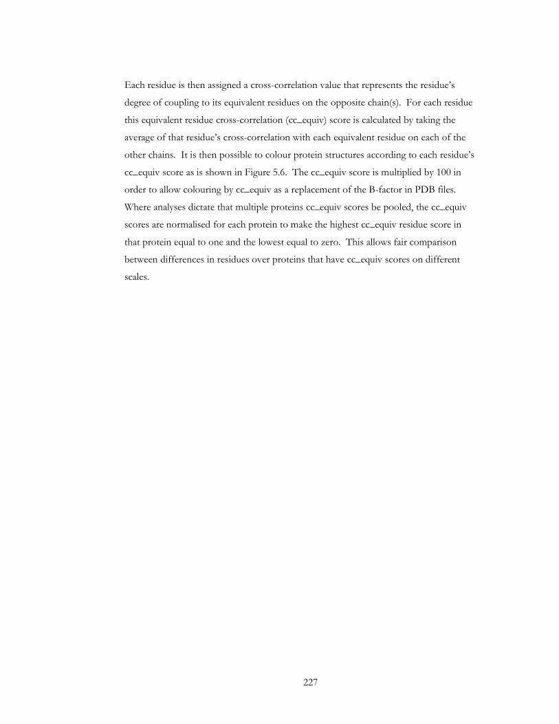
227

Each residue is then assigned a cross-correlation value that represents the residue’s

degree of coupling to its equivalent residues on the opposite chain(s). For each residue

this equivalent residue cross-correlation (cc_equiv) score is calculated by taking the

average of that residue’s cross-correlation with each equivalent residue on each of the

other chains. It is then possible to colour protein structures according to each residue’s

cc_equiv score as is shown in Figure 5.6. The cc_equiv score is multiplied by 100 in

order to allow colouring by cc_equiv as a replacement of the B-factor in PDB files.

Where analyses dictate that multiple proteins cc_equiv scores be pooled, the cc_equiv

scores are normalised for each protein to make the highest cc_equiv residue score in

that protein equal to one and the lowest equal to zero. This allows fair comparison

between differences in residues over proteins that have cc_equiv scores on different

scales.

228

Figure 5.6 The biological unit structure for 1D3V coloured according to each residue’s cc_equiv

score.

Residues coloured red are the most correlated residues in that structure, whereas dark blue are

the least correlated. The space-filled black atoms represent the ligand.

5.3 Correlated Residue Motions in Cooperative Oligomeric

Enzymes

The following work addresses whether active sites on the separate subunits in

cooperative enzymes have a higher degree of coupling between their dynamic

fluctuations than the active sites of non-cooperative enzymes. Cross-correlation scores

between each residue and their equivalent residue on the opposite chain (cc_equiv)

were calculated for all residues in proteins in Dataset 5.1 as discussed in 5.2. The

degree of correlation of equivalent residue fluctuations was compared for cooperative

and non-cooperative proteins and the results are shown below.

229

5.3.1 Analysis of Residue Correlations in Co-operative and Non

Cooperative Enzymes.

There are 17 positively cooperative, 4 negatively cooperative and 4 non-cooperative

proteins in the dataset for this analysis (Dataset 5.1). The average cc_equiv score for

site and non-site residues and the level of significance of the difference between them

(the Mann-Whitney p-value) is shown in Table 5.4. Where sites have a different

average cc_equiv (due to small changes in site residue annotation or symmetry) the

mean value is taken for all sites. The structure of each enzyme in the dataset is

coloured by each residues degree of cross-correlation with their equivalent residue

(positively cooperative enzymes are shown in Figure 5.7, negatively cooperative

enzymes are shown in Figure 5.8 and non-cooperative enzymes are shown in Figure

5.9).

230

Positively cooperative enzymes

1akm

1d3v

1egh

1eyj

1gbp

1ima

Continued overleaf.

231

1pwh

1u8f

1vgv

1xge

1xva

1y3i

Continued overleaf.

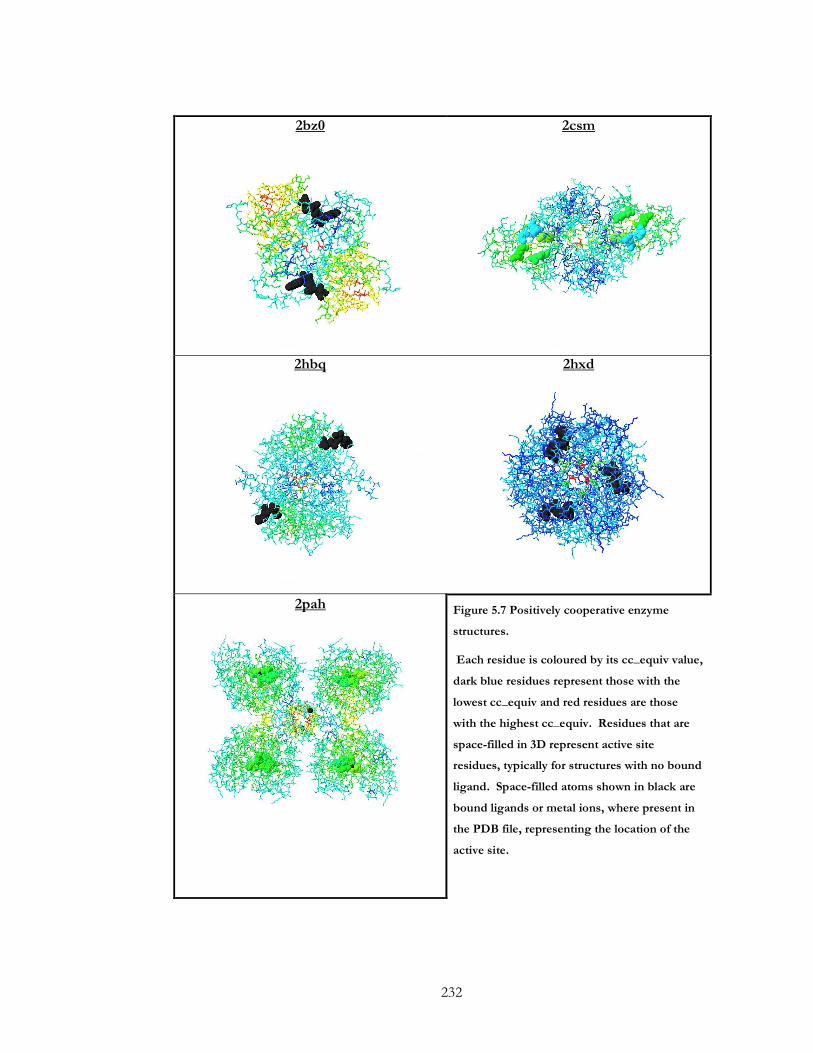
232

2bz0

2csm

2hbq

2hxd

2pah

Figure 5.7 Positively cooperative enzyme

structures.

Each residue is coloured by its cc_equiv value,

dark blue residues represent those with the

lowest cc_equiv and red residues are those

with the highest cc_equiv. Residues that are

space-filled in 3D represent active site

residues, typically for structures with no bound

ligand. Space-filled atoms shown in black are

bound ligands or metal ions, where present in

the PDB file, representing the location of the

active site.

233

Negatively cooperative enzymes

1pfk

1rv8

1xbt

2hgs

Figure 5.8 Negatively cooperative enzyme structures.

Each residue is coloured by its cc_equiv value, dark blue residues represent those with the

lowest cc_equiv and red residues are those with the highest cc_equiv. Space-filled atoms shown

in black are bound ligands or metal ions, where present in the PDB file, representing the

location of the active site.

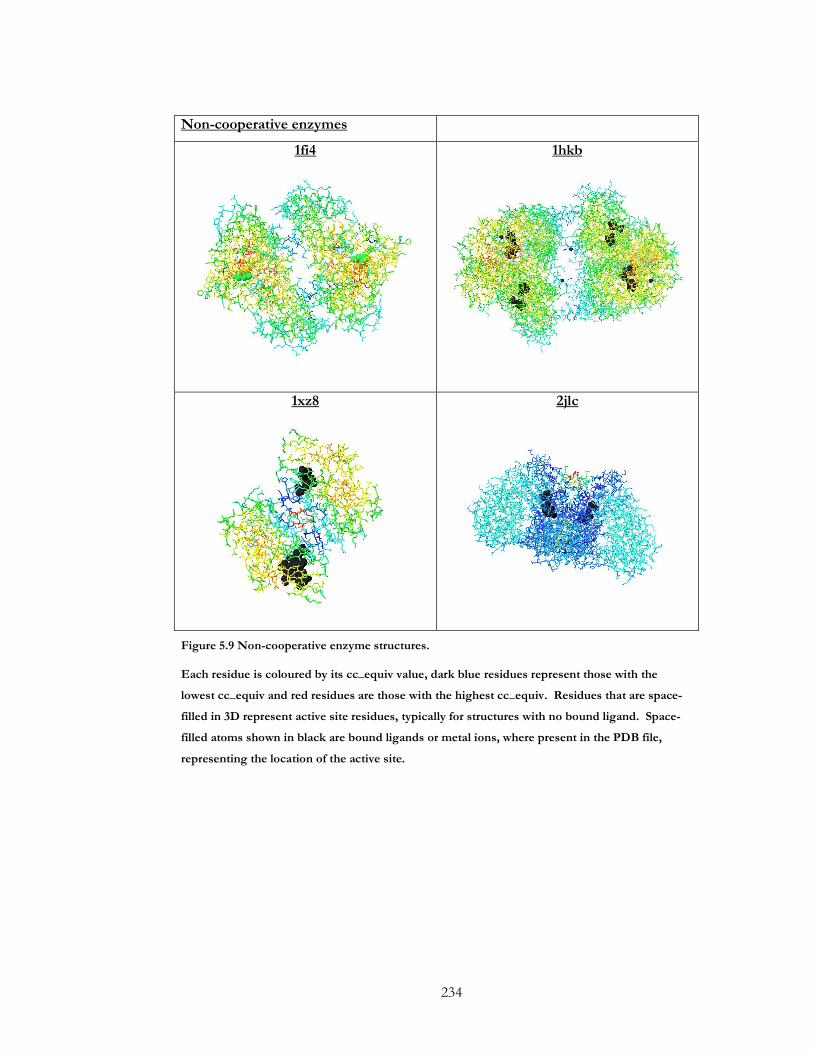
234

Non-cooperative enzymes

1fi4

1hkb

1xz8

2jlc

Figure 5.9 Non-cooperative enzyme structures.

Each residue is coloured by its cc_equiv value, dark blue residues represent those with the

lowest cc_equiv and red residues are those with the highest cc_equiv. Residues that are space-

filled in 3D represent active site residues, typically for structures with no bound ligand. Space-

filled atoms shown in black are bound ligands or metal ions, where present in the PDB file,

representing the location of the active site.

235

PDB Hill Coefficient Non-site average

cc_equiv Site average

cc_equiv Mann-Whitney

p-value

Positively cooperative 1egh 3.47 7.46 7.54 0.271

1akm 2.7 9.06 10.45 0.176

1xva 2.3 11.57 11.94 0.226

1d3v 2 11.16 13.31 0.023 1eyj 1.9 8.41 13.27 <0.001 2hxd 1.9 3.33 2.09 0.005 1ima 1.8 12.02 13.64 0.129

1vgv 1.8 18.89 18.59 0.956

1gpb 1.6 12.71 20.80 0.001 2csm 1.6 11.29 17.57 0.001 2pah 1.6 17.50 20.42 0.001 1xge 1.57 18.33 21.99 0.001 2hbq 1.5 9.54 11.74 0.028 1y3i 1.4 7.23 5.63 0.004 2bz0 1.3 12.83 8.15 0.002 1u8f 1.2 7.28 7.71 0.14

1pwh 1.12 18.35 21.44 <0.001

Negatively-cooperative 1pfk 0.8 5.77 5.36 0.316

1xbt 0.8 8.12 5.86 <0.001 2hgs 0.8 16.41 18.03 0.129

1rv8 0.32 15.60 20.82 0.059 Non-cooperative

1fi4* 1.07 21.37 23.44 0.602

1hkb 1 23.49 29.35 <0.001 1xz8 1 18.83 13.96 0.03 2jlc 1 8.16 5.19 0.024

Table 5.4 The average equivalent residue cross-correlation (cc_equiv) scores for site and non-

site residues for cooperative and non-cooperative enzymes.

The p-value (from Mann-Whitney tests) for the significance of the difference between the site

and non-site cc_equiv scores is also given. Enzymes shown in bold had a significant difference

between site and non-site cc_equiv values. * 1fi4 has a reported Hill coefficient of slightly more

than 1, but it is not significantly different than 1 and therefore has been defined as non-

cooperative.

The number of site residues defined by the criteria set out in 5.2.1 defines a relatively

small number of residues per site, particularly in cases where site residues are taken

from the CSA. The CSA annotates residues known to be involved in catalysis and so

other residues in the environment of the active site, but not involved in catalysis, are

not taken into account. Active sites that are in, or close to, highly correlated regions of

236

the structure yet have uncorrelated catalytic residues would therefore not show any

difference between active site and non-active site correlation. The centroid of the

active site was calculated from the site residues in the same way as described in 2.2.2

and the Spearman’s rank correlation coefficient between the distance from the active-

site centroid and the cc_equiv value was evaluated for each protein. The Spearman’s

rank correlation coefficient and its associated significance value for each enzyme are

given in Table 5.5.

Overall the majority (18 out of 25) of proteins has either a higher average active-site

cc_equiv value than the non-site residues or a negative correlation between cc_equiv

and the distance from the active site. Only 9 of the 17 cases where the average active

site cc_equiv is larger than non-active site cc_equiv values, however, are significant.

Enzymes for which their active sites show a significantly increased amount of

correlation in their dynamics exist in both the cooperative and non-cooperative sets.

Similarly, strong significant negative correlations exist between distance of a residue

from the active site centroid and its cc_equiv value for both cooperative and non-

cooperative enzymes.

Each enzyme has a different background distribution of cc_equiv values and so it

would be misleading to pool all cc_equiv values for site and non-site residues from

different proteins. The cc_equiv values were therefore scaled from 0 to 1 within each

enzyme before pooling residues from difference enzymes. Table 5.6 shows the mean

scaled cc_equiv values for all site and non-site residues in the cooperative (positive and

negative) and non-cooperative set. There is a non-significant increase in dynamic

correlation for site residues over non-site residues for cooperative enzymes, whereas

the increase is much larger (and significant) for non-cooperative enzymes.

Furthermore, the distribution of scaled cc_equiv values for site and non-site residues is

different for cooperative and non-cooperative proteins. Figure 5.10 shows that this

increase in dynamic correlation values over all residues for non-cooperative proteins is

also reflected in the raw cc_equiv values.

237

PDB Hill Coefficient Spearman's Rank Correlation Coefficient P-value

Positively cooperative

1egh 3.47 0.048 0.149

1akm 2.7 -0.070 0.029

1xva 2.3 -0.263 <0.001

1d3v 2 -0.361 <0.001

1eyj 1.9 -0.544 <0.001

2hxd 1.9 0.163 <0.001

1ima 1.8 -0.262 <0.001

1vgv 1.8 0.001 0.969

1gpb 1.6 -0.659 <0.001

2csm 1.6 -0.631 <0.001

2pah 1.6 -0.426 <0.001

1xge 1.57 -0.354 <0.001

2hbq 1.5 -0.366 <0.001

1y3i 1.4 0.172 <0.001

2bz0 1.3 0.349 <0.001

1u8f 1.2 -0.055 0.045

1pwh 1.12 -0.367 <0.001

Negatively-cooperative

1pfk 0.8 0.023 0.402

1xbt 0.8 -0.182 <0.001

2hgs 0.8 -0.378 <0.001

1rv8 0.32 -0.598 <0.001

Non-cooperative

1fi4* 1.07 -0.742 <0.001

1hkb 1 -0.663 <0.001

1xz8 1 0.113 0.042

2jlc 1 0.241 <0.001

Table 5.5 The Spearman’s rank correlation coefficient for the comparison between distance

from active site centroid and cc_equiv for each enzyme.

The level of significance associated with this correlation coefficient is also given. Residues in

enzymes that are given in red show no significant correlation between the distance from the

active site centroid and cc_equiv.

Cooperative (both positive and negative)

Non-cooperative

P-value (Cooperative vs. Non-cooperative)

Site residues 0.394 0.500

0.001

Non-site residues 0.388 0.440

<0.001

P-value (Site vs. Non-site) 0.436 0.018

Table 5.6 Average scaled cc_equiv values for pooled residues from enzymes within each set.

Mann-Whitney p-values are given for the differences in scaled cc_equiv values in each category.

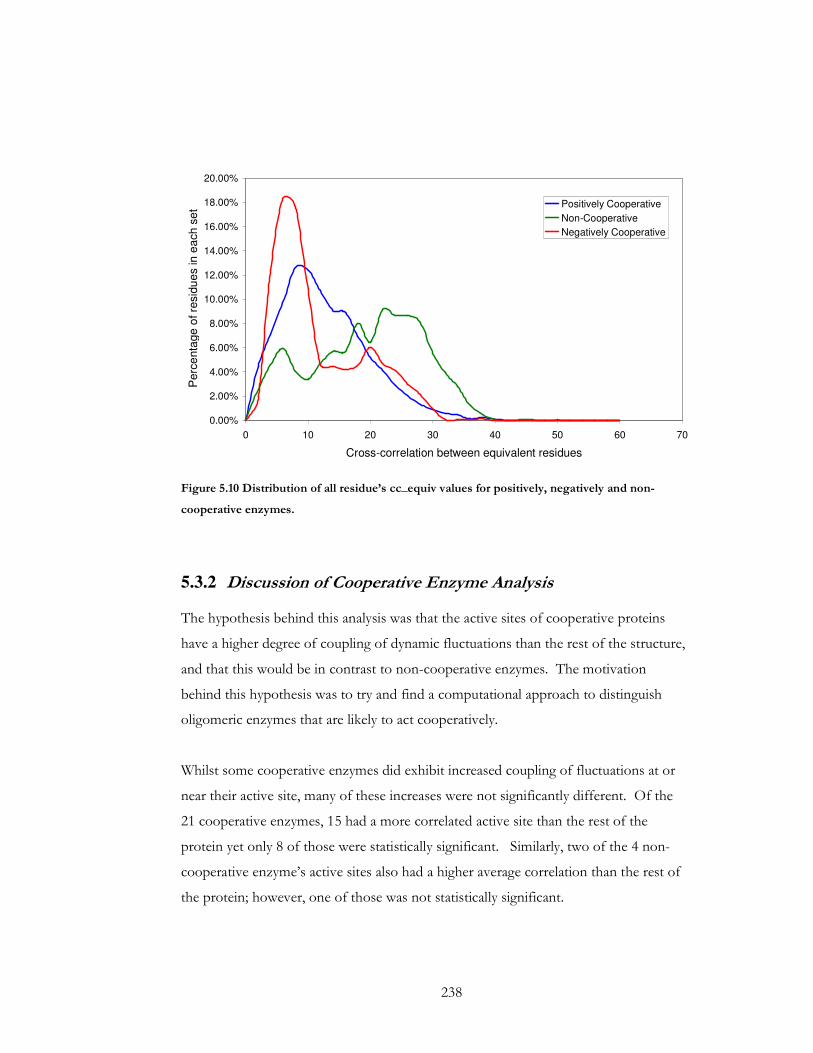
238

0.00%

2.00%

4.00%

6.00%

8.00%

10.00%

12.00%

14.00%

16.00%

18.00%

20.00%

0 10 20 30 40 50 60 70

Cross-correlation between equivalent residues

Perc

enta

ge

of re

sid

ue

s in

ea

ch s

et Positively Cooperative

Non-Cooperative

Negatively Cooperative

Figure 5.10 Distribution of all residue’s cc_equiv values for positively, negatively and non-

cooperative enzymes.

5.3.2 Discussion of Cooperative Enzyme Analysis

The hypothesis behind this analysis was that the active sites of cooperative proteins

have a higher degree of coupling of dynamic fluctuations than the rest of the structure,

and that this would be in contrast to non-cooperative enzymes. The motivation

behind this hypothesis was to try and find a computational approach to distinguish

oligomeric enzymes that are likely to act cooperatively.

Whilst some cooperative enzymes did exhibit increased coupling of fluctuations at or

near their active site, many of these increases were not significantly different. Of the

21 cooperative enzymes, 15 had a more correlated active site than the rest of the

protein yet only 8 of those were statistically significant. Similarly, two of the 4 non-

cooperative enzyme’s active sites also had a higher average correlation than the rest of

the protein; however, one of those was not statistically significant.

239

When the scaled cross-correlation values are pooled for cooperative and non-

cooperative proteins there is no significant difference between site and non-site

correlation for cooperative proteins, whereas non-cooperative proteins do seem to

exhibit higher site correlation values. Even without differentiating between site and

non-site residues, residues in non-cooperative enzymes seem to be more highly

correlated as a whole than in cooperative enzymes.

A major issue with this study is the small size of the dataset available. It is impossible

to identify any real trends in a dataset this small, particularly for non-cooperative

enzymes, of which there are only 4. The limitations of finding enzymes where there is

not only experimental evidence to support it acting cooperatively (or not) but also a

good quality structure from the same organism as the biochemical data is derived, is

prohibitive to forming a large dataset.

The pooled results (Figure 5.10 and Table 5.6), show that cc_equiv values tend to be

higher for site and non-site residues in non-cooperative proteins. This, however, may

be artificially skewed by two large non-cooperative enzymes in the small dataset. Out

of the 4 non-cooperative enzymes, two (1xz8 and 2jlc) have relatively small cc_equiv

values and have significantly less-correlated active sites than the rest of the protein,

whereas the remaining two (1fi4 and 1hkb) have relatively high cc_equiv values with

only one having a significantly higher-correlated active site than the rest of the protein.

It is therefore surprising that when the residues from the 4 enzymes are pooled they

show both a larger increase in active-site correlation over non-site residues and a higher

degree of correlation in general than non-cooperative proteins. This is due to the large

number of residues in the most highly-coupled enzyme, 1hkb (1834 residues),

dominating over the contributions from 1xz8, 2jlc and 1fi4 (which have 358, 1154 and

832 residues, respectively). This illustrates why it would be misleading to draw solid

conclusions from a dataset of this size.

The results from this limited dataset show that highly-correlated residue dynamic

fluctuations between active sites on different chains of oligomeric enzymes have not

been able to computationally identifying enzymes likely to act in a cooperative manner.

Further work is necessary to identify systematic links between computed correlations

and enzyme cooperativity/Hill coefficients.

240

5.4 Correlation of Residue Motions in Enzyme Active Site

Regions.

The results from the analysis of dynamic coupling in a very small set of cooperative

and non-cooperative enzymes show that the majority have either a higher average

active-site cc_equiv value than the non-site residues or a negative correlation between

cc_equiv and the distance from the active site. There was little distinction in this trend

between cooperative and non-cooperative enzymes and the small dataset size

prevented any solid conclusions to be reached. The suggestion from these results that

dynamic coupling may be a general feature of active sites in oligomeric enzymes,

regardless of their cooperative action, prompted a more extensive study of dynamic

coupling in a larger set of oligomeric enzymes with known active sites. A larger dataset

of oligomeric enzymes with known active sites was compiled as described in 5.2.2 and

the results are shown below.

5.4.1 Analysis of Residue Correlations in Enzyme Active Sites

The dataset described in 5.2.2 (Dataset 2.2) contains 114 homo-oligomeric enzymes

with literature annotated active site information. A similar analysis was carried out as

detailed in 5.3 for Dataset 2.2, this time looking to see whether active site residues were

significantly more highly-coupled with their equivalent residues on opposite chains

than non-active site residues for the whole set.

Due to the large number of proteins in this set results are mostly shown for pooled

data rather than per individual protein. Residue cc_equiv values were scaled between 0

and 1 within each enzyme, which allows fair comparison between differences in site

and non-site residues over enzymes with different background cc_equiv values. The

mean scaled cc_equiv value for pooled non-site residues is 0.362 and for site residues is

0.373. The Mann-Whitney p-value for the difference between non-site and site

cc_equiv values is <0.001 and the 95% confidence intervals are 0.360/0.363 and

0.367/0.379, respectively. This shows that active sites residues are significantly more

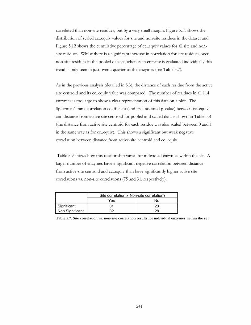
241

correlated than non-site residues, but by a very small margin. Figure 5.11 shows the

distribution of scaled cc_equiv values for site and non-site residues in the dataset and

Figure 5.12 shows the cumulative percentage of cc_equiv values for all site and non-

site residues. Whilst there is a significant increase in correlation for site residues over

non-site residues in the pooled dataset, when each enzyme is evaluated individually this

trend is only seen in just over a quarter of the enzymes (see Table 5.7).

As in the previous analysis (detailed in 5.3), the distance of each residue from the active

site centroid and its cc_equiv value was compared. The number of residues in all 114

enzymes is too large to show a clear representation of this data on a plot. The

Spearman’s rank correlation coefficient (and its associated p-value) between cc_equiv

and distance from active site centroid for pooled and scaled data is shown in Table 5.8

(the distance from active site centroid for each residue was also scaled between 0 and 1

in the same way as for cc_equiv). This shows a significant but weak negative

correlation between distance from active-site centroid and cc_equiv.

Table 5.9 shows how this relationship varies for individual enzymes within the set. A

larger number of enzymes have a significant negative correlation between distance

from active-site centroid and cc_equiv than have significantly higher active site

correlations vs. non-site correlations (75 and 31, respectively).

Site correlation > Non-site correlation?

Yes No

Significant 31 23

Non Significant 32 28

Table 5.7. Site correlation vs. non-site correlation results for individual enzymes within the set.

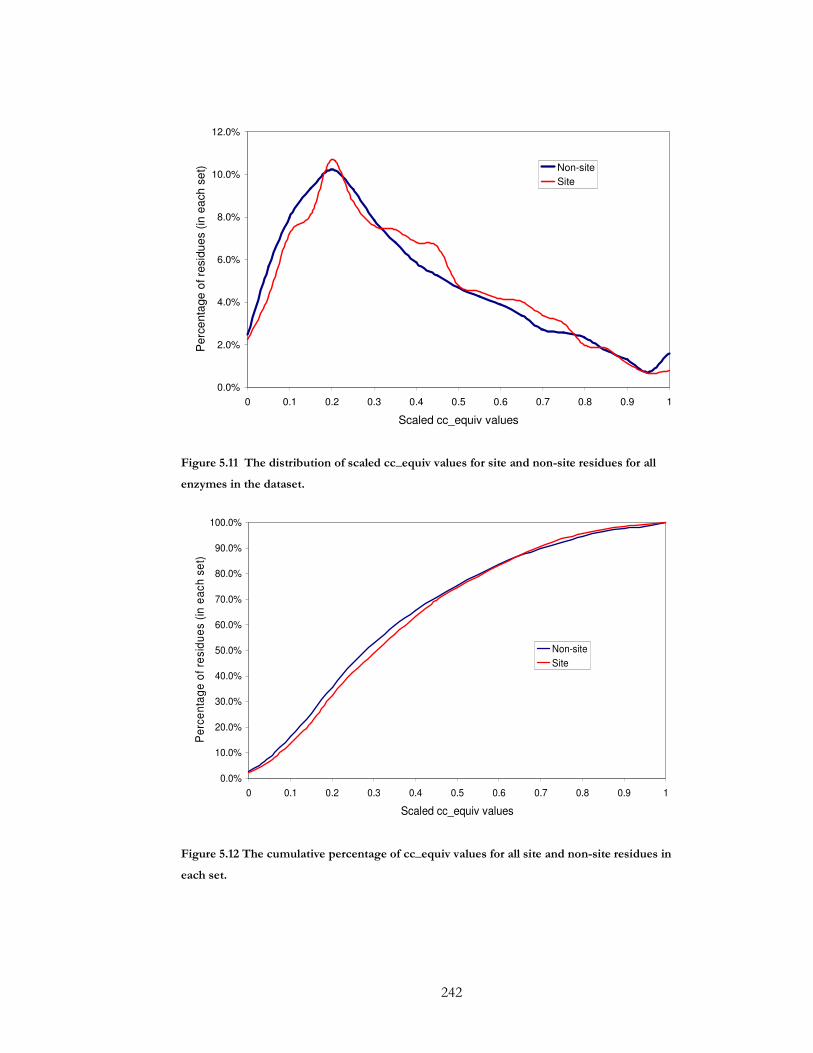
242

0.0%

2.0%

4.0%

6.0%

8.0%

10.0%

12.0%

0 0.1 0.2 0.3 0.4 0.5 0.6 0.7 0.8 0.9 1

Scaled cc_equiv values

Perc

enta

ge

of re

sid

ue

s (

in e

ach

se

t) Non-site

Site

Figure 5.11 The distribution of scaled cc_equiv values for site and non-site residues for all

enzymes in the dataset.

0.0%

10.0%

20.0%

30.0%

40.0%

50.0%

60.0%

70.0%

80.0%

90.0%

100.0%

0 0.1 0.2 0.3 0.4 0.5 0.6 0.7 0.8 0.9 1

Scaled cc_equiv values

Pe

rce

nta

ge

of

resid

ue

s (

in e

ach

se

t)

Non-site

Site

Figure 5.12 The cumulative percentage of cc_equiv values for all site and non-site residues in

each set.

243

Spearman's rank correlation coefficient P-value

-0.071 >0.001

Table 5.8 The Spearman’s rank correlation coefficient for the relationship between distance

from active site centroid and cc_equiv for all enzymes in the set.

Spearman's rank correlation coefficient

Negative Positive

Significant 75 25

Non-significant 8 6

Table 5.9 Table showing the breakdown of Spearman’s rank correlation coefficients between

distance from active site centroid and cc_equiv value for individual enzymes in the dataset.

A low B-factor (which approximates to the degree of structural constraint of a residue)

is a well documented feature of catalytic residues77; 78 and similarly the magnitude of

normal mode fluctuations has also been shown to be indicative of catalytic residues79.

It is a reasonable argument that residues in a constrained environment have a higher

probability of having more highly correlated motion with each other than those with

more freedom. If active site residues (which contain catalytic residues) tend to be more

constrained than other residues then this may explain their slight increase in fluctuation

correlation.

In this dataset only around half of the enzymes (58 out of 114) have a significantly

lower average B-factor for active site residues than non-site residues (see Table 5.10).

The Spearman’s rank correlation coefficient is significantly negative for the relationship

between cc_equiv and B-factor for 65 of the 114 enzymes in the dataset, indicating that

the hypothesis that more constrained residues are likely to be more highly correlated is

only supported for approximately half of the set (see Figure 5.11).

It is furthermore not the case that the enzymes where there are significantly higher

cc_equiv values in the active site (31 out of 114) are more likely to show significantly

lower B-factors or significantly negative relationships between cc_equiv and B-factor.

Table 5.12 shows that, as for the whole set, only around half of the enzymes where

active site residues are significantly more correlated than non-site residues have

244

significantly lower active-site B-factors and two-thirds have significant negative

relationships between cc_equiv and B-factor.

Number of proteins in the set

Higher average active site

B-factor than non-site Lower average active site

B-factor than non-site

Significant 18 58

Non-significant 9 29

Table 5.10 The number of proteins in the whole dataset that have either a lower or higher

average active site B-factor than non-site residues, split by significance.


Negative correlation between

B-factor and cc_equiv Positive correlation between

B-factor and cc_equiv

Significant 65 17


Table 5.11 The number of proteins in the whole dataset that have either a negative or positive

correlation between B-factor and cc_equiv, split by significance.

Number of proteins where the active site residues are

significantly more correlated than non-site residues

Higher average active site

B-factor than non-site Lower average active site

B-factor than non-site

Significant 6 16

Non-significant 2 7

Table 5.12 Number of proteins where the active site residues are significantly more correlated

than non-site residues that have either higher or lower average site B-factors in comparison to

the rest of the protein, split by significance.

Number of proteins where the active site residues are

significantly more correlated than non-site residues




Significant 20 4

Non-significant 5 2

Table 5.13 Number of proteins where the active site residues are significantly more correlated

than non-site residues that have either a positive or negative relationship between cc_equiv and

B-factor, split by significance.

245

5.4.2 Discussion of Correlation of Motion in Active Sites

It was the hypothesis that active site residues are at or near to parts of the enzyme

structure which have high correlation of residue fluctuations with their equivalent

residues in opposite chains. When scaled cc_equiv values are pooled for all enzymes in

the set there is a significant but small increase in cc_equiv values for site residues over

non-site residues. This trend however, only holds true for 31 of the 114 enzymes in

the set on an individual basis.

The motivation behind the hypothesis was to support identification of active sites in

oligomeric enzymes; however the very small overall difference in cc_equiv values over

the total dataset and the inconsistent pattern of active-site correlation values on an

individual basis suggests that it is not a promising candidate for use in characterising

active sites.

In contrast to the previous analysis, a problem in interpreting the results of this analysis

is due to the large number of data points (i.e. the total number of residues from all 114

enzymes) used to evaluate significance. Due to the large number of residues, very weak

correlation values are statistically significant. The Spearman’s rank correlation

coefficient (rho) for the relationship between B-factor and cc_equiv over the whole set

is very weakly negative (-0.071), which does not demonstrate a strong relationship

between these two features. Due to the large number of data points in the sample, the

threshold for rho to be significant is very low and therefore the above relationship is

statistically significant even though it is very weak.

Catalytic residues have been shown to have low B-factors78 and smaller magnitude of

normal mode fluctuations79 than other residues. It is a reasonable assumption that if a

residue is structurally constrained and the amount of space that its fluctuations can

sample is limited then it has a higher probability of being correlated with its equivalent

residues on the opposite chain. If this was true then it could explain the slight increase

in correlation between equivalent residues in active sites over non-active sites. Over all

residues in all enzymes in the dataset there was only a very weak (but significant)

negative correlation between cc_equiv and B-factor and only 65 out of 114 enzymes

246

showed a significant negative correlation on an individual basis. Of the 31 enzymes

that did show a significantly more correlated active site than the rest of the protein,

only half of these showed a significant negative relationship between cc_equiv and B-

factor, which suggests that for at least half of the cases where active sites are more

dynamically coupled that it is not the structural constraint of those residues that is

driving it.

5.5 Patterns of Correlation of Residue Motion as a

Structural Feature of Oligomeric Proteins

Correlations between residues within subunit structures have been shown to be of use

in characterising functional dynamics of protein structures80; 81; 82 but less is known

about how correlations across subunits affects the function of oligomers. Bai et al.,

observed that the overall degree of dynamic coupling was increased when a functional

dimer was considered in its oligomeric state rather than by considering the monomer

subunits separately83. This suggests that the oligomeric state of a protein has a

functional effect on its dynamic properties.

In the analyses in 5.3 and 5.4 the functional significance of these cross-subunit

fluctuation correlations was investigated. The first analysis failed to reach a solid

conclusion about whether active sites of cooperative enzymes have coupled motions

between subunits that are distinguishable from those of non-cooperative active sites.

Similarly, the previous analysis suggested only a slight increase in active site fluctuation

correlations between subunits in oligomers in general.

If the degree of coupling of a given residue with its equivalent residue on another

subunit isn’t associated with any functional or structural purpose for that enzyme, it

might be expected that either there is no variation in the degree of coupling between

different residues or that the variation is distributed in a random manor within the

structure. It is interesting, however, that the structures of enzymes in both analyses

tend to exhibit a broadly similar non-random architecture of coupling of residue

fluctuations.

The structures of oligomers coloured according to their per-residue cc_equiv value (see

Figure 5.7 to Figure 5.9 for enzymes from Dataset 2.1, for example) show a smooth,

247

ordered distribution of varying cross-subunit residue correlations over the protein

structure. The degree of correlation between equivalent residues appears from many of

these examples to organize itself into a common architecture. Highly-correlated

residues appear to assemble inside the subunit cores, with the surface of the subunit

exhibiting moderate cross-correlations and the subunit interfaces typically being the

least correlated.

If the assumption that tightly packed residues have a higher probability of their

fluctuations being coupled because of their limited freedom is true then it is perhaps

unsurprising that the cores of the subunits tend to be highly correlated with each other.

Given this hypothesis, however, the least packed residues- those on the surface of the

subunits- would be expected to show the lowest degree of coupling. It is therefore

interesting that surface residues appear to be more correlated than those in the

interface, even though such residues experience more structural constraint. It would

also be reasonable to assume that equivalent pairs that are the closest in the 3D

structure (as are the residues in the interface) would have higher-coupled motion than

those connected by longer range distances and so, again, it is surprising that interface

residues appear to be among the least correlated.

These observations are based on visual inspection of the relatively limited set of

enzymes in the previous analyses. To further investigate these observations, a new

dataset was created to include a wider range of homo-oligomeric proteins including

non-enzymes. The pattern of variation of cross-correlations within these structures

was evaluated quantitatively and the results are shown below.

5.5.1 Differences in Residue Motion Correlation According to

Structural Environment

The dataset used in this analysis (described in 5.2.3) contains 636 homo-oligomeric

proteins. As in previous analyses, the cc_equiv values were scaled from 0 to 1 within

each protein to enable residues from all proteins to be pooled. A structural

environment status (interface, core or surface) was assigned to each residue based on

the rules described in 5.2.3. The mean scaled cc_equiv values for each structural

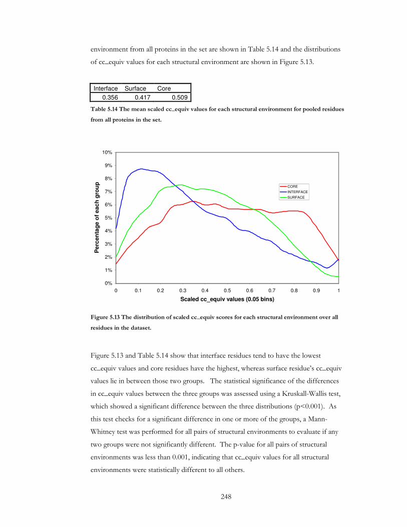
248

environment from all proteins in the set are shown in Table 5.14 and the distributions

of cc_equiv values for each structural environment are shown in Figure 5.13.

Interface Surface Core

0.356 0.417 0.509

Table 5.14 The mean scaled cc_equiv values for each structural environment for pooled residues

from all proteins in the set.

0%

1%

2%

3%

4%

5%

6%

7%

8%

9%

10%

0 0.1 0.2 0.3 0.4 0.5 0.6 0.7 0.8 0.9 1

Scaled cc_equiv values (0.05 bins)

Per

cen

tag

e o

f ea

ch g

rou

p

CORE

INTERFACE

SURFACE

Figure 5.13 The distribution of scaled cc_equiv scores for each structural environment over all

residues in the dataset.

Figure 5.13 and Table 5.14 show that interface residues tend to have the lowest

cc_equiv values and core residues have the highest, whereas surface residue’s cc_equiv

values lie in between those two groups. The statistical significance of the differences

in cc_equiv values between the three groups was assessed using a Kruskall-Wallis test,

which showed a significant difference between the three distributions (p<0.001). As

this test checks for a significant difference in one or more of the groups, a Mann-

Whitney test was performed for all pairs of structural environments to evaluate if any

two groups were not significantly different. The p-value for all pairs of structural

environments was less than 0.001, indicating that cc_equiv values for all structural

environments were statistically different to all others.

249

On an individual basis the majority of proteins (419) have lower average cc_equiv for

their interface residues than their surface and core residues, where the core residues

have the highest average cc_equiv. The core residues have the highest average

cc_equiv in 83% (529) of the dataset, and the interface has the lowest cc_equiv in 68%

of the proteins. The variation of cc_equiv values over the three structural

environments for individual proteins is shown in Table 5.15.


Interface 436 (392) 540 (490)

Surface 230 (142) 603 (533)

Core 96 (45) 33(6)

Table 5.15. Pairwise comparison of average cc_equiv values for each structural environment.

The value given is the number of proteins in the set where the average cc_equiv value for the

environment in the row is lower than the environment in the column. The figure in brackets is

the number of these cases where the difference is statistically significant.

The Spearman’s rank correlation coefficient for the relationship between the cc_equiv

score and the B-factor in this dataset shows a very weak negative correlation of -0.066

(p-value < 0.001). Table 5.16 shows the number of proteins in the dataset that have

either a negative or positive correlation between cc_equiv and B-factor (split by

significance).

The B-factors were scaled from 0 to 1 within each file to allow their distributions to be

compared over the whole set. The average scaled B-factor values for each structural

environment are shown in Table 5.17. The difference between B-factors in these three

environments is statistically significant for all pairs of environments (Mann-Whitney

p<0.001). The surface residues have the overall highest average B-factor and the core

residues have the lowest. Table 5.18 shows how differences in average B-factors for

each structural environment break down for individual proteins in the dataset. The

core residues have the highest average B-factors in over 90% of the proteins in the set,

and 88% have lower average B-factors for the interface than the surface.

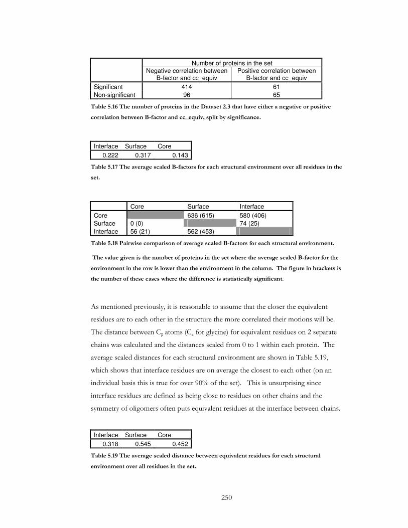
250





Significant 414 61


Table 5.16 The number of proteins in the Dataset 2.3 that have either a negative or positive

correlation between B-factor and cc_equiv, split by significance.


0.222 0.317 0.143

Table 5.17 The average scaled B-factors for each structural environment over all residues in the

set.

Core Surface Interface

Core 636 (615) 580 (406)

Surface 0 (0) 74 (25)

Interface 56 (21) 562 (453)

Table 5.18 Pairwise comparison of average scaled B-factors for each structural environment.

The value given is the number of proteins in the set where the average scaled B-factor for the

environment in the row is lower than the environment in the column. The figure in brackets is

the number of these cases where the difference is statistically significant.

As mentioned previously, it is reasonable to assume that the closer the equivalent

residues are to each other in the structure the more correlated their motions will be.

The distance between Cβ atoms (Cα for glycine) for equivalent residues on 2 separate

chains was calculated and the distances scaled from 0 to 1 within each protein. The

average scaled distances for each structural environment are shown in Table 5.19,

which shows that interface residues are on average the closest to each other (on an

individual basis this is true for over 90% of the set). This is unsurprising since

interface residues are defined as being close to residues on other chains and the

symmetry of oligomers often puts equivalent residues at the interface between chains.


0.318 0.545 0.452

Table 5.19 The average scaled distance between equivalent residues for each structural

environment over all residues in the set.

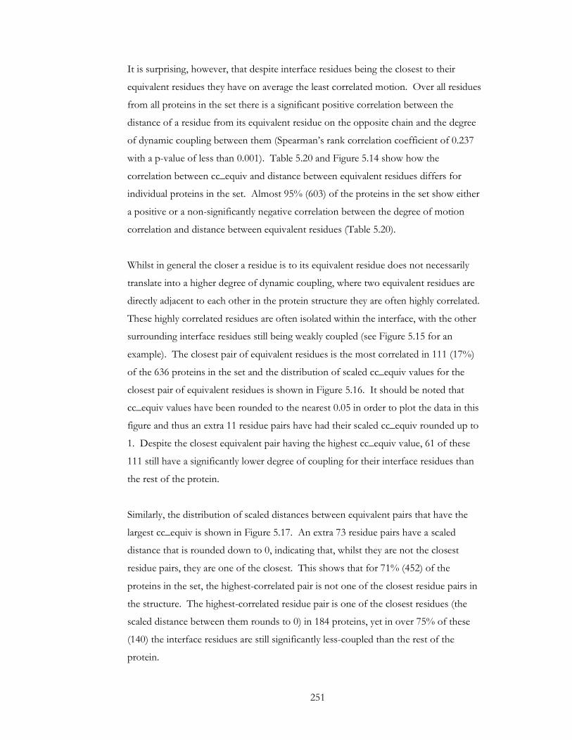
251

It is surprising, however, that despite interface residues being the closest to their

equivalent residues they have on average the least correlated motion. Over all residues

from all proteins in the set there is a significant positive correlation between the

distance of a residue from its equivalent residue on the opposite chain and the degree

of dynamic coupling between them (Spearman’s rank correlation coefficient of 0.237

with a p-value of less than 0.001). Table 5.20 and Figure 5.14 show how the

correlation between cc_equiv and distance between equivalent residues differs for

individual proteins in the set. Almost 95% (603) of the proteins in the set show either

a positive or a non-significantly negative correlation between the degree of motion

correlation and distance between equivalent residues (Table 5.20).

Whilst in general the closer a residue is to its equivalent residue does not necessarily

translate into a higher degree of dynamic coupling, where two equivalent residues are

directly adjacent to each other in the protein structure they are often highly correlated.

These highly correlated residues are often isolated within the interface, with the other

surrounding interface residues still being weakly coupled (see Figure 5.15 for an

example). The closest pair of equivalent residues is the most correlated in 111 (17%)

of the 636 proteins in the set and the distribution of scaled cc_equiv values for the

closest pair of equivalent residues is shown in Figure 5.16. It should be noted that

cc_equiv values have been rounded to the nearest 0.05 in order to plot the data in this

figure and thus an extra 11 residue pairs have had their scaled cc_equiv rounded up to

1. Despite the closest equivalent pair having the highest cc_equiv value, 61 of these

111 still have a significantly lower degree of coupling for their interface residues than

the rest of the protein.

Similarly, the distribution of scaled distances between equivalent pairs that have the

largest cc_equiv is shown in Figure 5.17. An extra 73 residue pairs have a scaled

distance that is rounded down to 0, indicating that, whilst they are not the closest

residue pairs, they are one of the closest. This shows that for 71% (452) of the

proteins in the set, the highest-correlated pair is not one of the closest residue pairs in

the structure. The highest-correlated residue pair is one of the closest residues (the

scaled distance between them rounds to 0) in 184 proteins, yet in over 75% of these

(140) the interface residues are still significantly less-coupled than the rest of the

protein.

252


Positive correlation between distance between equivalent

residues and cc_equiv

Negative correlation between distance between equivalent

residues and cc_equiv

Significant 418 87


Table 5.20 The number of proteins in the Dataset 2.3 that have either a negative or positive

correlation between the distance between equivalent residues and cc_equiv, split by

significance.

Figure 5.14 The distribution of Spearman’s rank correlation coefficients between cc_equiv

values and distance between equivalent residues for individual proteins in the dataset.

0

10

20

30

40

50

60

70

-1 -0.8 -0.6 -0.4 -0.2 0 0.2 0.4 0.6 0.8

Spearman's rank correlation coefficient between scaled cc_equiv values and distance between equivalent residues

Nu

mb

er

of

pro

tein

s

253

Figure 5.15 An example of a protein in the dataset (1h16) where the closest equivalent residues

in the interface have the highest dynamic coupling and the rest of the interface residues are less-

coupled in comparison.

Red residues have the highest cc_equiv value and dark blue have the lowest.

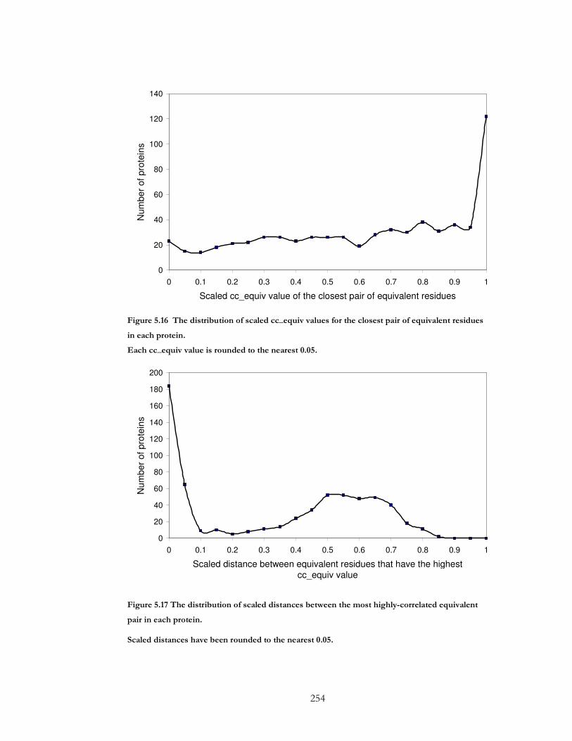
254

0

20

40

60

80

100

120

140

0 0.1 0.2 0.3 0.4 0.5 0.6 0.7 0.8 0.9 1

Scaled cc_equiv value of the closest pair of equivalent residues

Num

ber

of pro

tein

s

Figure 5.16 The distribution of scaled cc_equiv values for the closest pair of equivalent residues

in each protein.

Each cc_equiv value is rounded to the nearest 0.05.

0

20

40

60

80

100

120

140

160

180

200

0 0.1 0.2 0.3 0.4 0.5 0.6 0.7 0.8 0.9 1

Scaled distance between equivalent residues that have the highest cc_equiv value

Num

ber

of pro

tein

s

Figure 5.17 The distribution of scaled distances between the most highly-correlated equivalent

pair in each protein.

Scaled distances have been rounded to the nearest 0.05.

255

To investigate the extent to which the oligomeric status affects this common

architecture of correlated motion, the degree of correlation across subunits was

compared to the pattern of correlation of residue motion within subunits. The degree

of dynamic correlation of a residue to the all other residues within a single subunit was

estimated by averaging the correlation between a given residue and all other residues in

the subunit (termed the cc_within value). The distribution of Spearman’s correlation

coefficients between cc_equiv and cc_within values for each protein in the dataset is

shown in Figure 5.18. It shows that the patterns of variation of cc_equiv and

cc_within values over the structure are similar for most proteins.

0

20

40

60

80

100

120

140

-1.000 -0.800 -0.600 -0.400 -0.200 0.000 0.200 0.400 0.600 0.800 1.000

Sprearman's rank correlation coefficient between cc_within and

cc_equiv value

Num

ber

of pro

tein

s


cc_equiv values for all proteins in the set.

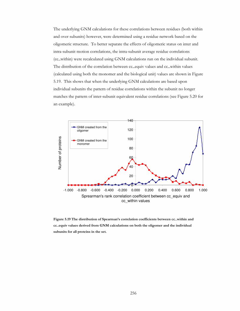
256

The underlying GNM calculations for these correlations between residues (both within

and over subunits) however, were determined using a residue network based on the

oligomeric structure. To better separate the effects of oligomeric status on inter and

intra-subunit motion correlations, the intra-subunit average residue correlations

(cc_within) were recalculated using GNM calculations run on the individual subunit.

The distribution of the correlation between cc_equiv values and cc_within values

(calculated using both the monomer and the biological unit) values are shown in Figure

5.19. This shows that when the underlying GNM calculations are based upon

individual subunits the pattern of residue correlations within the subunit no longer

matches the pattern of inter-subunit equivalent residue correlations (see Figure 5.20 for

an example).

0

20

40

60

80

100

120

140

-1.000 -0.800 -0.600 -0.400 -0.200 0.000 0.200 0.400 0.600 0.800 1.000

Sprearman's rank correlation coefficient between cc_equiv and

cc_within values

Nu

mb

er

of p

rote

ins

GNM created from theoligomer

GNM created from themonomer


cc_equiv values derived from GNM calculations on both the oligomer and the individual

subunits for all proteins in the set.

257

A

B

C

Figure 5.20 An example of a protein (1cq3) with residues coloured by cc_equiv value (A),

cc_within values derived using GNM calculations on the oligomer (B), and cc_within values

derived from GMN calculations on the individual monomers(C).

258

5.5.1.1 Are Residues with High Dynamic Coupling to their

Equivalent Residues more Evolutionarily Conserved?

The degree of evolutionary conservation was mapped onto each protein structure by

assigning each residue a conservation score (the methods for which are given in 3.3.1).

The conservation score was normalised from 0 to 1 within each protein structure. The

Spearman’s correlation coefficient between a residue’s normalised conservation score

and its cc_equiv value is plotted for each protein in the set (a conservation profile

could not be produced by PSI-BLAST for 21 of the proteins). Over all proteins the

correlation between conservation and the degree of dynamic coupling between

equivalent residues was 0.098 (p<0.001), which shows that there is only a weak positive

relationship between dynamic coupling and evolutionary conservation. Whilst it is true

that the core residues are generally the most conserved (and also have the highest

average cc_equiv values) the surface residues are the least conserved but do not have

the lowest average cc_equiv value (Table 5.21). Interface residues have the lowest

average cc_equiv value yet are evolutionarily conserved to a higher degree, therefore

only a weak positive relationship between conservation and degree of correlation of

motion exists.


0.339 0.258 0.385

Table 5.21 The average scaled conservation score for each structural environment.

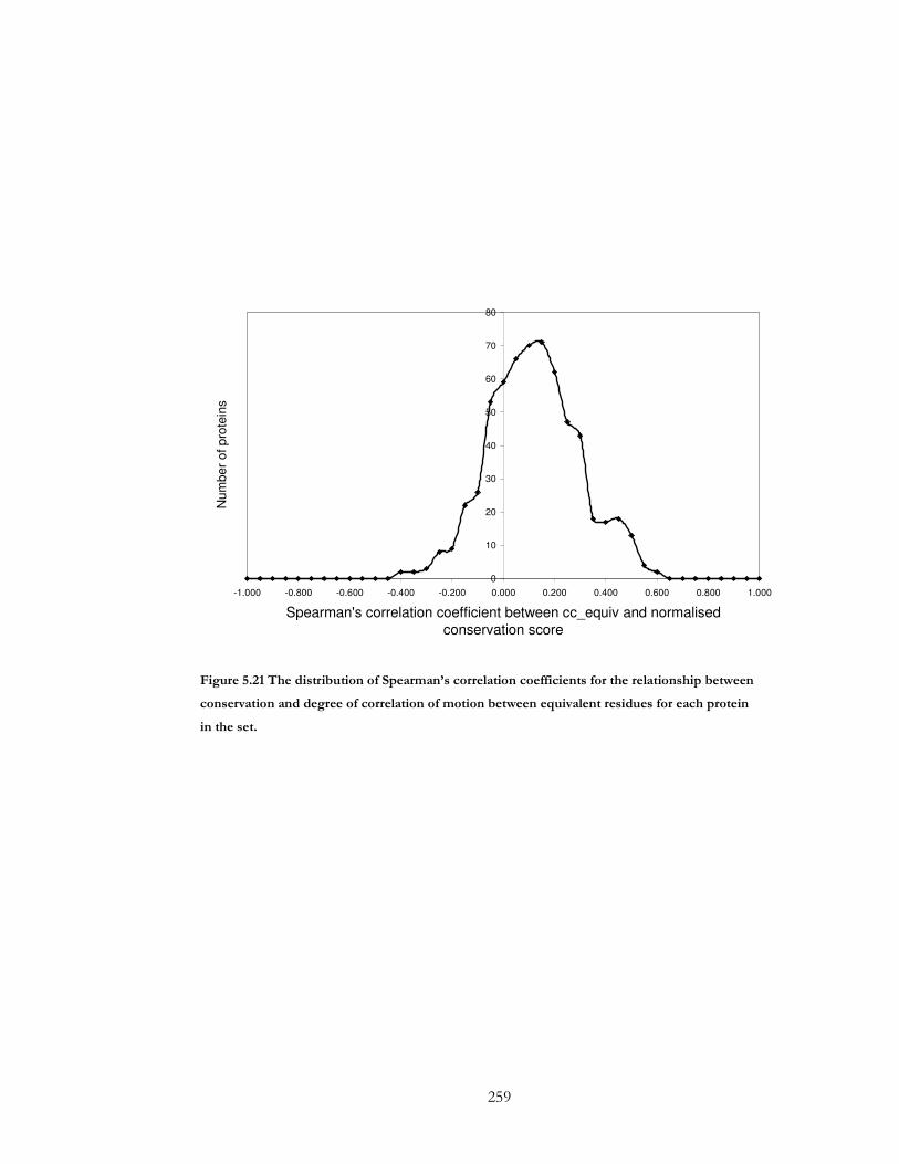
259

0

10

20

30

40

50

60

70

80

-1.000 -0.800 -0.600 -0.400 -0.200 0.000 0.200 0.400 0.600 0.800 1.000

Spearman's correlation coefficient between cc_equiv and normalised

conservation score

Num

be

r of pro

tein

s

Figure 5.21 The distribution of Spearman’s correlation coefficients for the relationship between

conservation and degree of correlation of motion between equivalent residues for each protein

in the set.

260

5.5.2 Discussion of Correlation of Motion According to Structural

Environment

As discussed previously, the degree of correlation of motion between pairs of residues

within subunits has been able to identify structural regions that relate to a protein’s

function80; 81; 82 but little is known about how much functional information is contained

in the correlation of motion between subunits. Cross-correlation matrices reveal

striking correlation patterns within subunits but these analyses show variation and order

in correlations across subunits, which is not obvious from these matrices (see Figure

5.22). If correlation of motion between subunits has no role in the structure or

function of a protein then it could be expected to either not vary, or vary in a random

pattern over the protein structure. This analysis shows that not only does the degree of

coupling over subunits vary for residues within a structure, but they seem to form a

common architecture where subunit cores are highly correlated, and subunit interfaces

are the lowest correlated.

It is possible that differences in the degree of dynamic coupling between equivalent

pairs are purely consequences of the constraints that their different environments place

on them. One such constraint, the degree of structural freedom of a residue’s side

chain (approximated by a residue’s B-factor), was investigated in the above analysis. If

the degree of structural constraint that a side chain experienced was solely responsible

for the variation in residue coupling then it would be expected that there would be a

strong negative correlation between B-factor and degree of coupling for proteins in the

set. It was shown, however, that only a very weak negative relationship existed

between these two variables (Spearman’s rank correlation coefficient = -0.066).

This small negative relationship was driven by core residues (which have the lowest

average B-factor) having the highest average degree of dynamic coupling. This was

however, contradicted by surface residues having the highest average B-factor but not

showing the smallest level of coupling. Despite experiencing a greater degree of

structural constraint than surface residues, the interface residues actually showed

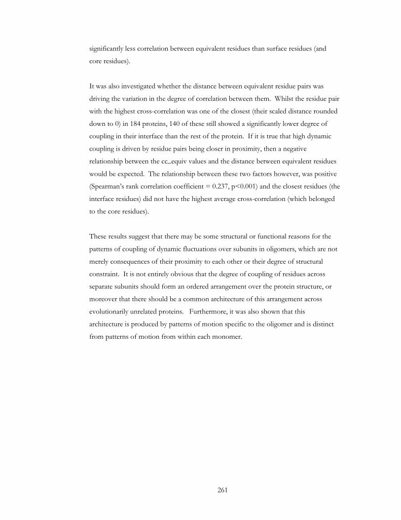
261

significantly less correlation between equivalent residues than surface residues (and

core residues).

It was also investigated whether the distance between equivalent residue pairs was

driving the variation in the degree of correlation between them. Whilst the residue pair

with the highest cross-correlation was one of the closest (their scaled distance rounded

down to 0) in 184 proteins, 140 of these still showed a significantly lower degree of

coupling in their interface than the rest of the protein. If it is true that high dynamic

coupling is driven by residue pairs being closer in proximity, then a negative

relationship between the cc_equiv values and the distance between equivalent residues

would be expected. The relationship between these two factors however, was positive

(Spearman’s rank correlation coefficient = 0.237, p<0.001) and the closest residues (the

interface residues) did not have the highest average cross-correlation (which belonged

to the core residues).

These results suggest that there may be some structural or functional reasons for the

patterns of coupling of dynamic fluctuations over subunits in oligomers, which are not

merely consequences of their proximity to each other or their degree of structural

constraint. It is not entirely obvious that the degree of coupling of residues across

separate subunits should form an ordered arrangement over the protein structure, or

moreover that there should be a common architecture of this arrangement across

evolutionarily unrelated proteins. Furthermore, it was also shown that this

architecture is produced by patterns of motion specific to the oligomer and is distinct

from patterns of motion from within each monomer.

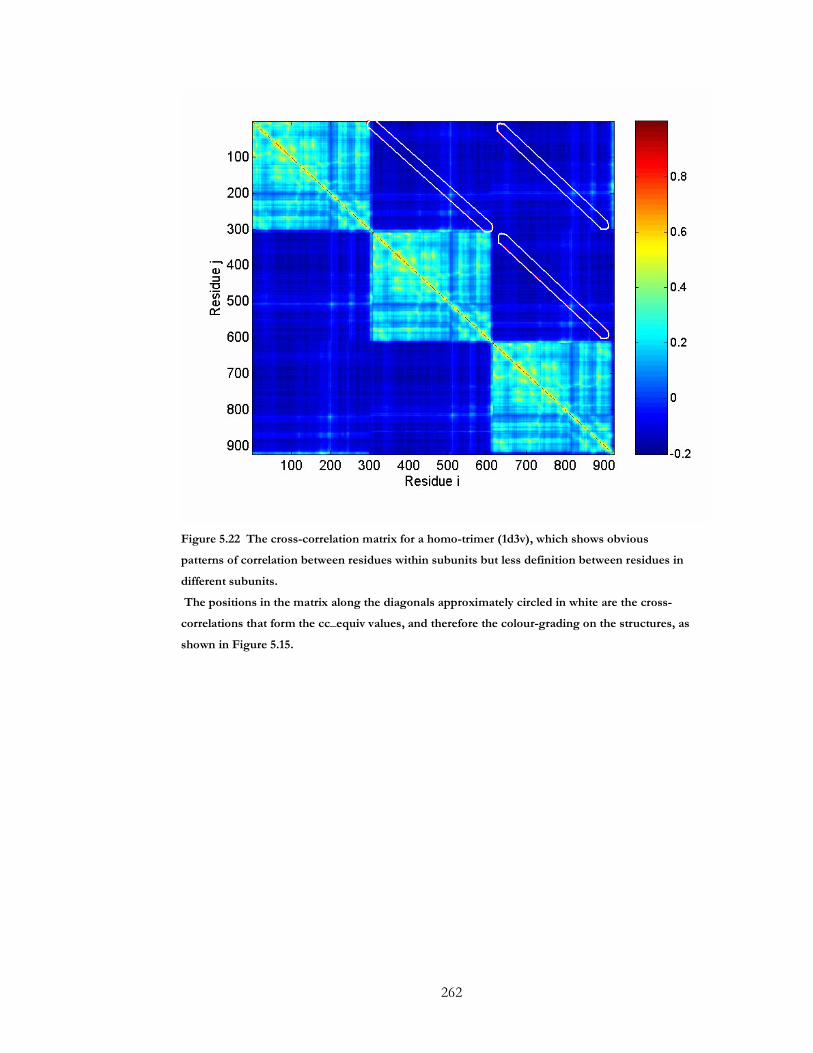
262

Figure 5.22 The cross-correlation matrix for a homo-trimer (1d3v), which shows obvious

patterns of correlation between residues within subunits but less definition between residues in

different subunits.

The positions in the matrix along the diagonals approximately circled in white are the cross-

correlations that form the cc_equiv values, and therefore the colour-grading on the structures, as

shown in Figure 5.15.

263

5.6 Conclusions

The initial aim of the work in this chapter was to assess whether dynamic coupling

between residues in the multiple active sites of cooperative proteins is distinguishable

from those in non-cooperative proteins. The intention of this work was to guide an

attempt to create a method to computationally identify enzymes which are likely to act

cooperatively from their structure. The results showed that the residues in active sites

of cooperative proteins are no more dynamically coupled than those in non-

cooperative proteins and thus, at present, is not able to successfully distinguish

cooperative and non-cooperative enzymes.

A number of observations whilst carrying out this work led to further analyses; firstly,

that active site regions appeared to be situated close to highly-coupled sections of the

enzyme structure and secondly, that the distribution of the degree of coupling between

equivalent residues on separate chains appeared to vary in an ordered manner over the

enzyme structure. These two observations were investigated further analyses on large

sets of non-redundant homo-oligomeric proteins.

The first of these analyses, which focused on the coupling of active site regions,

showed that over the whole dataset there is a statistically significant but very small

increase in the dynamic coupling of active site residues over non-active site residues in

homo-oligomeric enzymes. On an individual basis however, proteins within the set

were equally likely to have active sites with decreased coupling at their active sites than

increased coupling. Even for proteins with a significant increase in coupling in their

active sites, the magnitude of the difference is inadequate to distinguish active sites

residues from non-site residues.

The final analysis investigated the observation that oligomeric proteins, regardless of

the evolutionary relatedness, seemed to show a common architecture of the pattern of

coupling between equivalent residues over subunits of homo-oligomeric proteins. It

has been previously shown that similar architectures of protein folds exhibit similar

dynamics84 but here it is shown that dynamic coupling between subunits in homo-

oligomers is broadly conserved over a wide range of non-homologous proteins.

264

On a large, non-redundant set of homo-oligomeric proteins (including non-enzymes)

it was shown that the interface residues have the lowest distribution of cross-subunit

coupling, the core has the highest and the surface correlations fall in between. It is

perhaps surprising that interface residues are less correlated than others, particularly

due to their proximity to each other. It was also shown that the degree of constraint

was not responsible for the pattern of coupling, specifically as interfaces are generally

more tightly packed than surface residues yet they exhibit less coupling between them

than surface residues. Correlation of motion between residues within a subunit have

been shown to contain information relating to the protein’s function80; 81; 82 but little is

known about how residue motions are correlated over separate subunits and whether

these motions are important to the protein’s structure and function. A very weak

positive correlation was found between the evolutionary constraint of a residue and the

degree of correlation of motion to its equivalent residues, suggesting that evolution

does not necessarily act to preserve the most highly correlated motions over subunits

in the same way as has been suggested within subunits. The fact that the degree of

coupling over separate subunits varies in a smooth and ordered fashion over non-

homologous protein structures from a wide range of functions suggest that this pattern

of dynamics is functionally important to oligomeric proteins. It was shown that this

common architecture of dynamic coupling between residues is not intrinsic in the

monomer alone as it was altered in an inconsistent manner when the influence of the

oligomeric status was removed from the estimation of residue dynamics.

It is still unclear exactly what functional significance these cross-subunit dynamic

correlations have for oligomeric proteins. Perhaps the most plausible functionality that

correlated motion between subunits might bestow is communicating structural change

between distal residues for the purposes of cooperativity. An analysis of this concept

was attempted in this chapter and the results were inconclusive, especially due to the

availability of only a small number of biochemically-annotated structures. It is

possible that, due to the wide range of functions for which this pattern of coupling is

displayed, that the coupling is a structural feature of oligomeric proteins rather than

being associated with a particular function.

265

The dynamic coupling between interface residues is arguably the most important to the

viability of the oligomeric structural arrangement. Residue pairs on the surface, or even

in the core, can sample a variety of motion combinations without jeopardising the

overall quaternary structure. If, for example, a pair of interface residues was to move

in a correlated manor but in opposite directions, this could create a solvent-accessible

pocket in the subunit interface. The creation of a solvent-accessible pocket in an

interface would reduce the interaction energy between the two subunits and in turn,

potentially destabilise the quaternary structure. It is, therefore, reasonable to imagine

that the coupling between residue dynamics at the interface is selected to be more

chaotic and disorganised, and therefore less-correlated, to avoid creating solvent-

accessible space in the subunit interface, which would be detrimental to the

preservation of the quaternary structure.

266

5.7 References

1. Bohr C., H. K. A., Krogh A. (1904). Ueber einen in biologischer Beziehung wichtigen Einfluss, den die Kohlensäurespannung des Blutes auf dessen Sauerstoffbindung übt. Skand. Arch. Physiol 16, 402-412.

2. Hill, A. V. (1910). The possible effects of the aggregation of the molecules of hemoglobin on its dissociation curves. J. Physiol 40, iv-vii.

3. Goldbeter, A. & Koshland, D. E., Jr. (1981). An amplified sensitivity arising from covalent modification in biological systems. Proc Natl Acad Sci U S A 78, 6840-4.

4. Perutz, M. F. & Lehmann, H. (1968). Molecular pathology of human haemoglobin. Nature 219, 902-9.

5. Koshland, D. E., Jr. & Hamadani, K. (2002). Proteomics and models for enzyme cooperativity. In J Biol Chem, Vol. 277, pp. 46841-4.

6. Perutz, M. F. & Brunori, M. (1982). Stereochemistry of cooperative effects in fish an amphibian haemoglobins. Nature 299, 421-6.

7. Todd, A. E., Orengo, C. A. & Thornton, J. M. (2001). Evolution of function in protein superfamilies, from a structural perspective. J Mol Biol 307, 1113-43.

8. Thornton, J. M., Todd, A. E., Milburn, D., Borkakoti, N. & Orengo, C. A. (2000). From structure to function: approaches and limitations. Nat Struct Biol 7 Suppl, 991-4.

9. Bork, P. & Koonin, E. V. (1998). Predicting functions from protein sequences--where are the bottlenecks? Nat Genet 18, 313-8.

10. Iliopoulos, I., Tsoka, S., Andrade, M. A., Enright, A. J., Carroll, M., Poullet, P., Promponas, V., Liakopoulos, T., Palaios, G., Pasquier, C., Hamodrakas, S., Tamames, J., Yagnik, A. T., Tramontano, A., Devos, D., Blaschke, C., Valencia, A., Brett, D., Martin, D., Leroy, C., Rigoutsos, I., Sander, C. & Ouzounis, C. A. (2003). Evaluation of annotation strategies using an entire genome sequence. Bioinformatics 19, 717-26.

11. Go, N., Noguti, T. & Nishikawa, T. (1983). Dynamics of a small globular protein in terms of low-frequency vibrational modes. Proc Natl Acad Sci U S A 80, 3696-700.

12. Bahar, I., Atilgan, A. R. & Erman, B. (1997). Direct evaluation of thermal fluctuations in proteins using a single-parameter harmonic potential. Fold Des 2, 173-81.

13. Tirion, M. M. (1996). Large Amplitude Elastic Motions in Proteins from a Single-Parameter, Atomic Analysis. Phys Rev Lett 77, 1905-1908.

14. Atilgan, A. R., Durell, S. R., Jernigan, R. L., Demirel, M. C., Keskin, O. & Bahar, I. (2001). Anisotropy of fluctuation dynamics of proteins with an elastic network model. Biophys J 80, 505-15.

15. Tama, F. & Sanejouand, Y. H. (2001). Conformational change of proteins arising from normal mode calculations. Protein Eng 14, 1-6.

16. Li, G. & Cui, Q. (2002). A coarse-grained normal mode approach for macromolecules: an efficient implementation and application to Ca(2+)-ATPase. Biophys J 83, 2457-74.

17. Micheletti, C., Carloni, P. & Maritan, A. (2004). Accurate and efficient description of protein vibrational dynamics: comparing molecular dynamics and Gaussian models. Proteins 55, 635-45.

267

18. Doruker, P., Atilgan, A. R. & Bahar, I. (2000). Dynamics of proteins predicted by molecular dynamics simulations and analytical approaches: application to alpha-amylase inhibitor. Proteins 40, 512-24.

19. Ming, D., Kong, Y., Lambert, M. A., Huang, Z. & Ma, J. (2002). How to describe protein motion without amino acid sequence and atomic coordinates. Proc Natl Acad Sci U S A 99, 8620-5.

20. Van Wynsberghe, A., Li, G. & Cui, Q. (2004). Normal-mode analysis suggests protein flexibility modulation throughout RNA polymerase's functional cycle. Biochemistry 43, 13083-96.

21. Temiz, N. A. & Bahar, I. (2002). Inhibitor binding alters the directions of domain motions in HIV-1 reverse transcriptase. Proteins 49, 61-70.

22. Keskin, O., Bahar, I., Flatow, D., Covell, D. G. & Jernigan, R. L. (2002). Molecular mechanisms of chaperonin GroEL-GroES function. Biochemistry 41, 491-501.

23. Cui, Q., Li, G., Ma, J. & Karplus, M. (2004). A normal mode analysis of structural plasticity in the biomolecular motor F(1)-ATPase. J Mol Biol 340, 345-72.

24. Thomas, A., Hinsen, K., Field, M. J. & Perahia, D. (1999). Tertiary and quaternary conformational changes in aspartate transcarbamylase: a normal mode study. Proteins 34, 96-112.

25. Bahar, A. R. A., M.C. Demirel and B. Erman,. (1998). Dynamics of folded proteins: significance of slow and fast motions in relation to function and stability. Phys. Rev. Lett., 2733–2736.

26. Jernigan, R. L., Demirel, M.C., and Bahar, I. (1999). Relating structure to function through the dominant slow modes of motion of DNA topoisomerase II. Int. J. Quant. Chem.

27. Wang, Y., Rader, A. J., Bahar, I. & Jernigan, R. L. (2004). Global ribosome motions revealed with elastic network model. J Struct Biol 147, 302-14.

28. Xu, C., Tobi, D. & Bahar, I. (2003). Allosteric changes in protein structure computed by a simple mechanical model: hemoglobin T<-->R2 transition. J Mol Biol 333, 153-68.

29. Ming, D. & Wall, M. E. (2005). Allostery in a coarse-grained model of protein dynamics. Phys Rev Lett 95, 198103.

30. Kundu, S., Sorensen, D. C. & Phillips, G. N., Jr. (2004). Automatic domain decomposition of proteins by a Gaussian Network Model. Proteins 57, 725-33.

31. Bahar, I., Wallqvist, A., Covell, D. G. & Jernigan, R. L. (1998). Correlation between native-state hydrogen exchange and cooperative residue fluctuations from a simple model. Biochemistry 37, 1067-75.

32. Micheletti, C., Lattanzi, G. & Maritan, A. (2002). Elastic properties of proteins: insight on the folding process and evolutionary selection of native structures. J Mol Biol 321, 909-21.

33. Kundu, S., Melton, J. S., Sorensen, D. C. & Phillips, G. N., Jr. (2002). Dynamics of proteins in crystals: comparison of experiment with simple models. Biophys J 83, 723-32.

34. Yang, L. W., Rader, A. J., Liu, X., Jursa, C. J., Chen, S. C., Karimi, H. A. & Bahar, I. (2006). oGNM: online computation of structural dynamics using the Gaussian Network Model. Nucleic Acids Res 34, W24-31.

35. Suhre, K. & Sanejouand, Y. H. (2004). ElNemo: a normal mode web server for protein movement analysis and the generation of templates for molecular replacement. Nucleic Acids Res 32, W610-4.

268

36. Hollup, S. M., Salensminde, G. & Reuter, N. (2005). WEBnm@: a web application for normal mode analyses of proteins. BMC Bioinformatics 6, 52.

37. Tobi, D. & Bahar, I. (2005). Structural changes involved in protein binding correlate with intrinsic motions of proteins in the unbound state. Proc Natl Acad Sci U S A 102, 18908-13.

38. Cooper, A. & Dryden, D. T. (1984). Allostery without conformational change. A plausible model. Eur Biophys J 11, 103-9.

39. Tama, F., Gadea, F. X., Marques, O. & Sanejouand, Y. H. (2000). Building-block approach for determining low-frequency normal modes of macromolecules. Proteins 41, 1-7.

40. Barthelmes, J., Ebeling, C., Chang, A., Schomburg, I. & Schomburg, D. (2007). BRENDA, AMENDA and FRENDA: the enzyme information system in 2007. Nucleic Acids Res 35, D511-4.

41. Wittig U., G., M., Kania, R., Krebs, O., Mir, S., Weidemann, A., Anstein, S., Saric, J. and Rojas, I. (2006). SABIO-RK: Integration and Curation of Reaction Kinetics Data. In Data Integration in the Life Sciences, Vol. 4075, pp. 94-103. Springer Berlin / Heidelberg.

42. Milo, R., Hou, J. H., Springer, M., Brenner, M. P. & Kirschner, M. W. (2007). The relationship between evolutionary and physiological variation in hemoglobin. Proc Natl Acad Sci U S A 104, 16998-7003.

43. Daily, M. D. & Gray, J. J. (2007). Local motions in a benchmark of allosteric proteins. Proteins 67, 385-99.

44. Kanehisa, M., Goto, S., Hattori, M., Aoki-Kinoshita, K. F., Itoh, M., Kawashima, S., Katayama, T., Araki, M. & Hirakawa, M. (2006). From genomics to chemical genomics: new developments in KEGG. Nucleic Acids Res 34, D354-7.

45. Yang, Y. R. & Schachman, H. K. (1993). In vivo formation of active aspartate transcarbamoylase from complementing fragments of the catalytic polypeptide chains. Protein Sci 2, 1013-23.

46. Kuo, L. C., Lipscomb, W. N. & Kantrowitz, E. R. (1982). Zn(II)-induced cooperativity of Escherichia coli ornithine transcarbamoylase. Proc Natl Acad Sci U S A 79, 2250-4.

47. Wang, X. G. & Engel, P. C. (1995). Positive cooperativity with Hill coefficients of up to 6 in the glutamate concentration dependence of steady-state reaction rates measured with clostridial glutamate dehydrogenase and the mutant A163G at high pH. Biochemistry 34, 11417-22.

48. Kikonyogo, A., Abriola, D. P., Dryjanski, M. & Pietruszko, R. (1999). Mechanism of inhibition of aldehyde dehydrogenase by citral, a retinoid antagonist. Eur J Biochem 262, 704-12.

49. Maggini, S., Stoecklin-Tschan, F. B., Morikofer-Zwez, S. & Walter, P. (1992). New kinetic parameters for rat liver arginase measured at near-physiological steady-state concentrations of arginine and Mn2+. Biochem J 283 ( Pt 3), 653-60.

50. Saadat, D. & Harrison, D. H. (1998). Identification of catalytic bases in the active site of Escherichia coli methylglyoxal synthase: cloning, expression, and functional characterization of conserved aspartic acid residues. Biochemistry 37, 10074-86.

51. Nelson, S. W., Honzatko, R. B. & Fromm, H. J. (2004). Origin of cooperativity in the activation of fructose-1,6-bisphosphatase by Mg2+. J Biol Chem 279, 18481-7.

269

52. Krepkiy, D. & Miziorko, H. M. (2004). Identification of active site residues in mevalonate diphosphate decarboxylase: implications for a family of phosphotransferases. Protein Sci 13, 1875-81.

53. Sergienko, E. A. & Srivastava, D. K. (1997). Kinetic mechanism of the glycogen-phosphorylase-catalysed reaction in the direction of glycogen synthesis: co-operative interactions of AMP and glucose 1-phosphate during catalysis. Biochem J 328 ( Pt 1), 83-91.

54. Dunaway, G. A., Jr. & Smith, E. C. (1971). A comparative study of some of the enzymes involved in glucose metabolism of human diploid and SV40-transformed human diploid cells. Cancer Res 31, 1418-21.

55. Ganzhorn, A. J., Lepage, P., Pelton, P. D., Strasser, F., Vincendon, P. & Rondeau, J. M. (1996). The contribution of lysine-36 to catalysis by human myo-inositol monophosphatase. Biochemistry 35, 10957-66.

56. Foster, B. A., Thomas, S. M., Mahr, J. A., Renosto, F., Patel, H. C. & Segel, I. H. (1994). Cloning and sequencing of ATP sulfurylase from Penicillium chrysogenum. Identification of a likely allosteric domain. J Biol Chem 269, 19777-86.

57. Calcagno, M., Campos, P. J., Mulliert, G. & Suastegui, J. (1984). Purification, molecular and kinetic properties of glucosamine-6-phosphate isomerase (deaminase) from Escherichia coli. Biochim Biophys Acta 787, 165-73.

58. Auzat, I., Le Bras, G. & Garel, J. R. (1994). The cooperativity and allosteric inhibition of Escherichia coli phosphofructokinase depend on the interaction between threonine-125 and ATP. Proc Natl Acad Sci U S A 91, 5242-6.

59. Hsieh, J. Y., Chen, S. H. & Hung, H. C. (2009). Functional roles of the tetramer organization of malic enzyme. J Biol Chem 284, 18096-105.

60. Lopez-Flores, I., Barroso, J. B., Valderrama, R., Esteban, F. J., Martinez-Lara, E., Luque, F., Peinado, M. A., Ogawa, H., Lupianez, J. A. & Peragon, J. (2005). Serine dehydratase expression decreases in rat livers injured by chronic thioacetamide ingestion. Mol Cell Biochem 268, 33-43.

61. Sauve, V. & Sygusch, J. (2001). Molecular cloning, expression, purification, and characterization of fructose-1,6-bisphosphate aldolase from Thermus aquaticus. Protein Expr Purif 21, 293-302.

62. Diaz, A., Munoz-Clares, R. A., Rangel, P., Valdes, V. J. & Hansberg, W. (2005). Functional and structural analysis of catalase oxidized by singlet oxygen. Biochimie 87, 205-14.

63. Samuel, J. & Tanner, M. E. (2004). Active site mutants of the "non-hydrolyzing" UDP-N-acetylglucosamine 2-epimerase from Escherichia coli. Biochim Biophys Acta 1700, 85-91.

64. Frederiksen, H., Berenstein, D. & Munch-Petersen, B. (2004). Effect of valine 106 on structure-function relation of cytosolic human thymidine kinase. Kinetic properties and oligomerization pattern of nine substitution mutants of V106. Eur J Biochem 271, 2248-56.

65. Lee, M., Chan, C. W., Mitchell Guss, J., Christopherson, R. I. & Maher, M. J. (2005). Dihydroorotase from Escherichia coli: loop movement and cooperativity between subunits. J Mol Biol 348, 523-33.

66. Konishi, K. & Fujioka, M. (1988). Rat liver glycine methyltransferase. Cooperative binding of S-adenosylmethionine and loss of cooperativity by removal of a short NH2-terminal segment. J Biol Chem 263, 13381-5.

67. Chander, P., Halbig, K. M., Miller, J. K., Fields, C. J., Bonner, H. K., Grabner, G. K., Switzer, R. L. & Smith, J. L. (2005). Structure of the nucleotide complex

270

of PyrR, the pyr attenuation protein from Bacillus caldolyticus, suggests dual regulation by pyrimidine and purine nucleotides. J Bacteriol 187, 1773-82.

68. Raffaelli, N., Finaurini, L., Mazzola, F., Pucci, L., Sorci, L., Amici, A. & Magni, G. (2004). Characterization of Mycobacterium tuberculosis NAD kinase: functional analysis of the full-length enzyme by site-directed mutagenesis. Biochemistry 43, 7610-7.

69. Ritz, H., Schramek, N., Bracher, A., Herz, S., Eisenreich, W., Richter, G. & Bacher, A. (2001). Biosynthesis of riboflavin: studies on the mechanism of GTP cyclohydrolase II. J Biol Chem 276, 22273-7.

70. Schnappauf, G., Strater, N., Lipscomb, W. N. & Braus, G. H. (1997). A glutamate residue in the catalytic center of the yeast chorismate mutase restricts enzyme activity to acidic conditions. Proc Natl Acad Sci U S A 94, 8491-6.

71. Scheer, J. M., Romanowski, M. J. & Wells, J. A. (2006). A common allosteric site and mechanism in caspases. Proc Natl Acad Sci U S A 103, 7595-600.

72. Njalsson, R., Carlsson, K., Bhansali, V., Luo, J. L., Nilsson, L., Ladenstein, R., Anderson, M., Larsson, A. & Norgren, S. (2004). Human hereditary glutathione synthetase deficiency: kinetic properties of mutant enzymes. Biochem J 381, 489-94.

73. Bjornberg, O., Neuhard, J. & Nyman, P. O. (2003). A bifunctional dCTP deaminase-dUTP nucleotidohydrolase from the hyperthermophilic archaeon Methanocaldococcus jannaschii. J Biol Chem 278, 20667-72.

74. Bhasin, M., Billinsky, J. L. & Palmer, D. R. (2003). Steady-state kinetics and molecular evolution of Escherichia coli MenD [(1R,6R)-2-succinyl-6-hydroxy-2,4-cyclohexadiene-1-carboxylate synthase], an anomalous thiamin diphosphate-dependent decarboxylase-carboligase. Biochemistry 42, 13496-504.

75. Bjorgo, E., de Carvalho, R. M. & Flatmark, T. (2001). A comparison of kinetic and regulatory properties of the tetrameric and dimeric forms of wild-type and Thr427-->Pro mutant human phenylalanine hydroxylase: contribution of the flexible hinge region Asp425-Gln429 to the tetramerization and cooperative substrate binding. Eur J Biochem 268, 997-1005.




79. Yang, L. W. & Bahar, I. (2005). Coupling between catalytic site and collective dynamics: a requirement for mechanochemical activity of enzymes. Structure 13, 893-904.

80. Ma, W., Tang, C. & Lai, L. (2005). Specificity of trypsin and chymotrypsin: loop-motion-controlled dynamic correlation as a determinant. Biophys J 89, 1183-93.

81. Keskin, O., Durell, S. R., Bahar, I., Jernigan, R. L. & Covell, D. G. (2002). Relating molecular flexibility to function: a case study of tubulin. Biophys J 83, 663-80.

82. Bahar, I., Erman, B., Jernigan, R. L., Atilgan, A. R. & Covell, D. G. (1999). Collective motions in HIV-1 reverse transcriptase: examination of flexibility and enzyme function. J Mol Biol 285, 1023-37.

271

83. Bai, H., Ma, W., Liu, S. & Lai, L. (2008). Dynamic property is a key determinant for protein-protein interactions. Proteins 70, 1323-31.

84. Keskin, O., Jernigan, R. L. & Bahar, I. (2000). Proteins with similar architecture exhibit similar large-scale dynamic behavior. Biophys J 78, 2093-106.

272

Chapter 6: Conclusions

The work included in this thesis broadly addresses aspects of how structure relates to

function in proteins (for most of the thesis this specifically relates to enzymes). The

initial aim of the project was to improve prediction of EC class from structural and

sequence features of enzymes by including active-site specific features. In working

towards this aim, the general relationships between these features and the functions of

each EC class were explored in Chapter 2. This involved identifying features that

differ significantly between the six EC classes and further analysing those that showed

the most significant differences.

Three features that showed significant differences between EC classes were

investigated further; these included the proportion of non-polar residues in the active

site, the proportion of aspartic acid in the active site and the number of residues in the

biological unit (which relates to the oligomeric status). The proportion of the active

site composed of non-polar residues was one of the most significantly-different

features between the six classes. The oxidoreductases (EC1) exhibited the highest

proportion of non-polar residues in the active sites. Oxidoreductases are the most

likely group of enzymes to elicit their function by binding a cofactor and these

cofactors often contain large non-polar groups. Upon removing the cofactor-binding

proteins from the whole dataset the composition of the active site that is non-polar was

reduced for the oxidoreductases and there was no longer a significant different

between the six classes.

The active site composition of aspartic acid was also one of the most significantly-

different features between the six EC classes. The aspartic acid active site composition

was the lowest for the oxidoreductases. The reduction in aspartic acid composition for

oxidoreductases was compensated by a preference for glutamic acid. This was

surprising since aspartic acid is preferred as an active site (and catalytic) residue over

glutamic acid, which is seen in the other five classes. Glutamic acid has different

hydrogen-bonding properties to aspartic acid and it was shown that Glu residues form

significantly more hydrogen bonds in oxidoreductases, than in other classes and also

significantly more than aspartic acid. It was suggested that Glu is preferred to Asp in

273

order to form hydrogen bond networks in the active site that play a role in proton

shuffling, the most common catalytic mechanism of the oxidoreductases.

Further work to investigate this hypothesis would include structural bioinformatics and

experimentation. For example, the static calculations of hydrogen-bonding reported in

this thesis could be extended with calculations of alternate rotameric forms in networks

of sidechains, particularly where pathways for proton transfer have been suggested in

the literature. The aim would be to examine whether swapping Asp for Glu impedes

these pathways through restriction of alternate hydrogen-bonded networks. The same

question could be asked experimentally, with mutagenesis and substitution of Glu and

Asp sidechains, alongside a read-out of catalytic activity.

Lastly, the number of residues in the biological unit structures differed significantly

between the functional classes. The lyases (EC4) had the largest number of residues in

the biological unit, but not the largest average/median sequence length. This suggested

that the differences in size were due to differences in oligomeric status. Indeed, lyases

were the class most likely to form high-order oligomers (three or more chains). It was

also found that lyases were also more likely to active sites at, or near to, subunit

boundaries. It was suggested that they form high-order oligomers to allow finely-tuned

control of their action since lyases were also found to be over-represented at important

points in metabolic networks. Conversely, the hydrolases were the smallest and

preferred to exist as monomers and were also under-represented at important points in

metabolic networks.

Lyases may prefer to exist in high-order oligomers in order to allow cooperative action

between subunits in order to elicit a high level of control over their catalytic action.

Since biochemical data is incomplete for much of the dataset, a method to

computationally identify oligomeric enzymes that act cooperatively was needed.

Chapter 5 starts by analysing the degree of coupling of residue motion between

oligomers in an attempt to distinguish oligomers that act cooperatively than those that

do not. Whilst this method was unable to distinguish between cooperative and non-

cooperative oligomers, it was observed that the pattern of correlation between residue

motion is broadly conserved over a large number of oligomers. This was further

274

identified in a large, functionally diverse, non-redundant set of oligomeric protein

structures.

Since the role of protein dynamics in function is receiving increasing attention, it will

be important to investigate further the observation of a common pattern of correlated

motion at interfaces. In purely computational terms, there is scope for more complex

analysis of the normal modes than reported in this thesis, for example examining the

role of individual lower frequency modes, which are generally expected to play

important roles in functional properties.

In order to address the original aim of this thesis, to improve EC class prediction by

the addition of sequence and structural features of the active site region, it was

necessary to use an active site prediction method in order to identify active sites in

proteins that may have no functional annotation. Many computational tools have been

developed to predict functional sites of proteins and it was considered out of the scope

of this project to develop one. Chapter 3 contains a thorough benchmark analysis of

current publicly-available functional site prediction tools in order to identify the best-

performing method to be used in subsequent function prediction methods. We found

that, alongside another tool (Consurf) a previous method developed by the Warwicker

group (SitesIdentify) predicted enzyme active sites and functional sites of non-enzymes

with the highest accuracy. This method was not previously publicly-available and so

Chapter 3 also presents the creation of a web-server to deliver the SitesIdentify method

via the web.

Lastly, structural and sequence features of enzymes, including those relating to their

active sites, were used to create a method to predict the top EC class of an enzyme

without the transfer of information via homology. The first attempt used a vector

comparison method on enzymes with known active sites. Whilst this did not achieve a

high level of accuracy it was more than expected by chance, which indicates that the

features used in the model held information that was indicative of the top EC function

in enzymes. It was a further improvement on increase in accuracy than obtained by

previous attempts by this group using a similar method without including active site

features. This suggested that features specific to the active site increase the model’s

ability to predict function. A further approach in this chapter used a larger set of

enzymes with predicted active site locations to calculate features. Prediction models

275

were made using a machine learning approach (SVMs) and achieved a similar level of

accuracy.

The levels of accuracy and lack of balance in the EC class prediction methods limit

their use in real-world function prediction problems. In order to increase prediction

accuracy then it is possible that the model needs to be updated to include alternative

prediction features such as electrostatic profiles, particularly of active sites. Other

machine learning approaches, such as Random forests may display better utility for this

particular prediction problem. Random forests are a collection of decision trees, where

the prediction is the most popular output from individual trees. Trees are constructed

using a random subset of variables at each branch point. The advantages of such a

method are that it can handle large number of input features and can give indications

of the level of importance of these in making the predictions.

Predicting EC class is obviously only applicable to enzymes, and it becomes necessary

to therefore predict beforehand whether the protein is an enzyme or non-enzyme.

This introduces a further level of error in predicting the correct function of the protein.

It also does not aid in predicting the functions of non-enzymes. It would, therefore,

also be useful to construct prediction models based on classification schemes that do

not only apply to enzymes, such as the Gene Ontology (GO). Despite the limitation of

the applicability of this EC class prediction model, it gives a quantitative indication of

how well the differences in features described in Chapter 2 are predictive of EC class.

Even without prediction, there is still much to be learnt from understanding how

structural and sequence features relate to functional class and why evolutionary diverse

but functionally similar proteins can exhibit similar features.

FROM STRUCTURE TO FUNCTION IN PROTEINS: A …

Documents

Transcript of FROM STRUCTURE TO FUNCTION IN PROTEINS: A …