From linear to nonlinear control means: a practical...

ISATRA 1158p Disk used

UNCORREC

TEDPR

OOF

DTD=4.2.0Version 7, No. pages 14

From linear to nonlinear control means:a practical progression

Zhiqiang Gao*

Department of Electrical and Computer Engineering, Cleveland State University, Cleveland, OH 44115, USA

Received 21 November 2000; accepted 18 April 2001

Abstract

With the rapid advance of digital control hardware, it’s time to take the simple but effective PID control technology tothe next level of performance and robustness. For this purpose, a nonlinear PID and active disturbance rejection fra-mework are introduced in this paper. It compliments the existing theory in that: (1) it actively and systematically explores

the use of nonlinear control mechanisms for better performance, even for linear plants; (2) it represents a control strategythat is rather independent of mathematical models of the plants, thus achieving inherent robustness and reducing designcomplexity. Stability analysis, as well as software/hardware test results, are presented. It is evident that the proposed

framework lends itself well in seeking innovative solutions to practical problems while maintaining the simplicity andthe intuitiveness of the existing technology. # 2001 Published by Elsevier Science Ltd. All rights reserved.

Keywords: PID; Nonlinear PID; Disturbance observer; Approximate differentiation

1. Introduction

The proportional-integral-derivative (PID) basedexisting control technology has been in existence forclose to 80 years. N. Minorsky first invented it in1922 [1]. Ziegler and Nichols provided a set of tun-ing tables that has been used to this day [2]. Variouscontrol forms and tuning methods related to PIDhave continued to appear in literature, see forexample [4–8]. Nevertheless, the PID is still thetool of choice in over 90% of current industrialcontrol applications [3].

Classical control theory, particularly the fre-quency response method, helps control engineersto get helpful insight on how and why feedbackcontrol system works, as well as how to improveit. Modern control theory, from Kalman Filters toH1 control, represents the tremendous progressmade in the last 40 years in mathematical controltheory. But the level of mathematics required tounderstand it, the assumptions of linearity andtime invariance, and its dependency on the math-ematical model of the physical plant has limited itsappeal for most control practitioners.

Judging from the state of control technology, itseems that the development in control theory hasnot been translated to a breakthrough technology.In the meanwhile, the control industry has com-pleted the transition from analog to digital and is

0019-0578/01/$ - see front matter # 2001 Published by Elsevier Science Ltd. All rights reserved.

PI I : S0019-0578(01 )00027-1

ISA Transactions & (&&&&) &–&www.elsevier.com/locate/isatrans

* Tel.: +1-216-687-3528; fax: +1-216-687-5405.

E-mail address: [email protected]

1

2

3

4

5

6

7

8

9

10

11

12

13

14

15

16

17

18

19

20

21

22

23

24

25

26

27

28

29

30

31

32

33

34

35

36

37

38

39

40

41

42

43

44

45

46

47

48

49

50

51

52

53

54

55

56

57

58

59

60

61

62

63

64

65

66

67

68

69

70

71

72

73

74

75

76

77

78

79

80

81

82

83

84

85

86

87

88

89

90

91

92

93

94

95

96


UNCORREC

TEDPR

OOF


capable of implementing much more sophisticatedalgorithms than PID. But where is our next gen-eration control technique that can tap into thepower of the new digital control hardware?

This paper proposes a new vision on controltechnology progression. Keep in mind that thenew technology

. should not be overly dependent on themathematical model since they are oftenunavailable in practice

. needs to provide much better performance atlow cost

. must be intuitive and simple to implement

It is in this background that several novel designmethods are presented here. Some of these ideas,such as the use of nonlinear gains, have been uti-lized, in one form or the other, by practicing engi-neers as ad hoc solutions but were not systematicallystudied. The pioneering work of Professor JingqingHan’s in nonlinear control [9–15] provided a muchneeded framework for the study of such techni-ques.

In the following sections, several novel andpractical design techniques, including nonlinearPID mechanisms and an innovative active dis-turbance rejection scheme, are presented. Practicalapplications are used to demonstrate their applic-ability and effectiveness. Note that this research isby no means complete. Instead, it points to a pro-mising new direction of control technology devel-opment: break out from the constraints of theexisting control practice and theory, and activelyexplore new control design strategies that are notoverly dependent on mathematical models. Com-pute aided design tools, such Matlab/Simulink,provide an ideal environment for such endeavorswhere new ideas can be quickly tested. In fact, thisis how the proposed techniques presented herewere first developed.

2. Nonlinear PID control mechanisms

Engineers have long used various modificationsof PID, from gain scheduling to fuzzy logic, inpractice. The nonlinear variations usually providemuch needed improvements of performance and

flexibility of the controller. However, the designprocess tends to be tedious and solutions problemdependent. In this section, a systematic nonlinearPID design approach is proposed. It leads to simple,effective and practical control solutions that applyto a wide range of industrial control problems.

2.1. Nonlinear proportional-integral control

Consider a single integrator plant

y:¼ wþ u ð1Þ

with y and u as the output and input, respectively,and w as input disturbance. For convenience, theequation is written in terms of the error, e=r�y,where r is the desired output (constant)

e:¼ �w� u ð2Þ

The objective is to design a control law such thatthe closed-loop system satisfies e(t) ! 0, as t !

1. In practice, in the presence of the disturbancew, a proportional-integral (PI) control is usuallyemployed:

u ¼ Kpeþ KI

ðedt ð3Þ

It is well known that the integrator control helpsto eliminate steady-state error. Unfortunately, itoften causes saturation problems (known as inte-grator windup) and its 90� phase lag may adverselyaffect system stability. For these reasons, it is notuncommon to see that the integral control is gain-scheduled in practice. For example, a commonpractice is to zero the integral gain during the tran-sient to prevent overshoot, saturation, and instabil-ity. This and other variations of PID are theresults of ingenuities of practicing engineers. But, ascontrol researchers, can we provide them with amore powerful set of tools that are less problematic?Let’s start the investigation by examining a novelbuilding block of a controller: a nonlinear gain.

2.1.1. Nonlinear proportional controlIntuitively, the reason integral control helps to

reduce the steady state error is that it makes thecontroller more sensitive to small errors. This

2 Z. Gao / ISA Transactions & (&&&&) &–&

1

2

3

4

5

6

7

8

9

10

11

12

13

14

15

16

17

18

19

20

21

22

23

24

25

26

27

28

29

30

31

32

33

34

35

36

37

38

39

40

41

42

43

44

45

46

47

48

49

50

51

52

53

54

55

56

57

58

59

60

61

62

63

64

65

66

67

68

69

70

71

72

73

74

75

76

77

78

79

80

81

82

83

84

85

86

87

88

89

90

91

92

93

94

95

96


UNCORREC

TEDPR

OOF


compliments the proportional control actions. Analternative is to use a nonlinear mechanism in thecontroller that yields higher gain for smallererrors, such as the one below:

u ¼ K ej jasign eð Þ ð4Þ

which was systematically used by Han [12–14] toexplore the advantage of nonlinear feedback. Thesign(e) function is defined as:

sign eð Þ ¼1 e50�1 e < 0

�

Note that for a=0 and 1, (4) represents the well-known bang-bang control and the linear propor-tional control, respectively. It is in the case of0<a<1 where an interesting phenomenon wasobserved. The selection of the parameter a isstudied in terms of steady-state error, transientresponse, disturbance rejection, and robustness, asshown below.

2.1.1.1. Steady-state error. For the same gain ofK=10, when w0j j < 1, 8 t, the steady-state error isless than 0.1 for the linear controller with a=1, and0.01 for the nonlinear controller with a=1/2. Thisbound is further reduced to 0.001 with a=1/3. Ingeneral, as a!0, this bound will approach zero.

2.1.1.2. Transient response. With K=10, the tran-sient responses are for a=0, 1=2, 1, are shown inFig. 1. Note that the linear control has the slowestresponse because it has a long tail end. This is dueto its inherent nature of not being sensitive tosmall errors. On the other hand, the bang-bangcontrol has the fastest response but the chatteringin the control signal renders it impractical. Thenonlinear control with 0<a<1 seems to offer agood balance.

2.1.1.3. The choice of gain. Note that from Fig. 1,the gain K corresponds to the maximum controleffort. Since the output never overshoots the tar-get, the control signal is limited to the range of[0,K], for a>0. That is, the control gain can beconveniently chosen from the physical limitationof actuator.

2.1.1.4. Implication in hardware simplification.Keeping the control signal always positive arequite significant in applications where negativecontrol signal requires a different set of hardware.For example, in temperature applications, thepositive control signal means heating and thenegative one cooling. The above results imply thatwith a proper control strategy that produces fastresponse without overshoot, the cooling actuatormaybe not be needed even for an aggressive con-trol design with 0<a<1. In drive applications, itmay result in a motor drive that never applies thereversed torque, which not only helps to saveenergy, but also prolongs the life of motor andother parts in the drive train, such as coupling andtransmission.

2.1.1.5. Disturbance rejection. To examine the dis-turbance rejection properties of linear and nonlinearcontrollers, a disturbance of w(t)=2+sin(10t) isintroduced. The results are shown in Fig. 2 for a=1,1=2, 1/5. Again, the linear control is the least desir-able one.

2.1.1.6. Robustness. Let us examine the robustnessof the control law in (4) with respect to thedynamic changes in the plant (1). Consider a firstorder system with a time constant �:

�y:¼ �yþ wþ u ð5Þ

Fig. 1. Comparison of the linear and nonlinear controllers.

Z. Gao / ISA Transactions & (&&&&) &–& 3

1

2

3

4

5

6

7

8

9

10

11

12

13

14

15

16

17

18

19

20

21

22

23

24

25

26

27

28

29

30

31

32

33

34

35

36

37

38

39

40

41

42

43

44

45

46

47

48

49

50

51

52

53

54

55

56

57

58

59

60

61

62

63

64

65

66

67

68

69

70

71

72

73

74

75

76

77

78

79

80

81

82

83

84

85

86

87

88

89

90

91

92

93

94

95

96


UNCORREC

TEDPR

OOF


With the same controller (K=10, a=1/2) andthe disturbance, w0(t)=2+sin(10t), used above, �is varied from 0.1 to 1. The results are shown inFig. 3. It is demonstrated that the high quality ofcontrol is maintained even though the pole of thesystem shifted significantly.

2.1.1.7. Remarks. (1)The reason the nonlinearcontroller performs better is that, with 0< � < 1,it provides higher gain when error is small andlower gain when error is large. It completelyagrees with the intuition obtained from workingwith practical problems. As a matter of fact, manyfuzzy logic controllers exhibit this kind of char-acteristics on its error surface. Of course a fuzzycontroller is much more complicated to imple-ment. (2) The above study demonstrates a desir-

able characteristic of nonlinear control: reducingthe steady state error in the presence of dis-turbances does not necessarily require an integralcontrol. This helps to enhance the stability mar-gins of the control system by eliminating the phasedelay associated with integral control. The controlimplementation is also simplified by removing theanti-windup mechanisms that is used to preventthe integrator from saturation. (3) In some appli-cations, the physical plant exhibits high gain incertain operating conditions. In this case, theNPID concept should be applied so that the com-bined gain of the controller and the process hasthe shape of Fig. 4. This may require that thecontroller gain be actually small when the error issmall, which is evident in the pH level regulationproblems in process control.

2.1.2. StabilityMany industrial control problems, such as the

drive systems and thermo processes are approxi-mately described by first order linear differentialequation as

y:¼ ��yþ wþ bu ð6Þ

with �>0 and b>0, and w is the disturbance. But,considering many different nonlinear behaviorsexhibited by physical devices, such as the dead-zone, the hysteresis and backlash, and the differentforms of frictions, a better representation is

y:¼ �f y;wð Þ þ bu ð7Þ

where f(y,w) accounts for the nonlinear dynamicsand disturbances in the system.

Fig. 3. Robustness of the nonlinear controller. Fig. 4. Comparison of linear and nonlinear gains with a<1.

Fig. 2. Disturbance rejection comparisons.


1

2

3

4

5

6

7

8

9

10

11

12

13

14

15

16

17

18

19

20

21

22

23

24

25

26

27

28

29

30

31

32

33

34

35

36

37

38

39

40

41

42

43

44

45

46

47

48

49

50

51

52

53

54

55

56

57

58

59

60

61

62

63

64

65

66

67

68

69

70

71

72

73

74

75

76

77

78

79

80

81

82

83

84

85

86

87

88

89

90

91

92

93

94

95

96


UNCORREC

TEDPR

OOF


For the sake of simplicity, the disturbance, w, isignored in the stability analysis. Note that althoughf(y) is often unknown in practice, it usually sharesthe same sign of y, i.e. yf(y) 50. Furthermore, theconstant b generally has explicit physical meaningsand is within a certain range. It represents animportant relationship of how an actuator affectsthe system dynamically. For example, b corre-sponds to the torque constant of the motor in adrive system.

It was demonstrated above that the nonlinearfeedback control law, such as

u ¼ �K y�� asign yð Þ ð8Þ

is a very effective one. The question addressed hereis if the stability of the closed-loop system can beassured with a limited knowledge of the plant.

Theorem 1. The proposed control law in (8) guar-antees the asymptotic stability of the closed-loopsystem if K is chosen such that

bK > supy

f yð Þ�� y�� a

!ð9Þ

Proof. Select the Lyapunov function VðyÞ ¼ y2=2.

V:yð Þ ¼ yy

:¼ �yf yð Þ � bKy y

�� asign yð Þ

¼ �yf yð Þ � bK y�� aþ1

a) If yfðyÞ50, and bK>0, then

V:yð Þ < 0 for y 6¼ 0:

b) If yfðyÞ < 0, and bK>0 then for V:yð Þ<0 one

needs

bK y�� aþ1

> yf yð Þ��

or equivalently

bK > supy

f yð Þ�� y�� a Q:E:D:

&

2.1.3. The design trade-offsThe control law in (4) provides a relatively high

gain when error is small, which leads to smallsteady-state error, good disturbance rejection androbustness. However, this high gain is sustainedacross the frequency spectrum and pushes thebandwidth of the controller upwards, which maymake the controller too sensitive to noises. Since thegain of the controller in (4) increases as the error getssmaller, one possible trade-off is to limit the gainto a particular value. For example, changing (4) to

uK fal eð Þ ð10Þ

where the function fal(e), shown in Fig. 4, isdefined as:

fal eð Þ ¼ej jasign eð Þ; ej j > d;e=d1�a; ej j4d;

d > 0

�ð11Þ

which limits the gain to K/d1-a in the neighborhoodof origin. This proves to be a very effective methodin making a compromise between the effectivenessof the nonlinear control and the bandwidth andnoise sensitivities of the control algorithm.

Another trade-off that can further lower thegain is adding an integral control in the neighbor-hood of steady-state. In particular, the integralcontrol helps to eliminate the steady state errorwithout using high gain proportion control. Fur-thermore, the saturation and phase lag problemscan be avoided, or at least lessened, by applying theintegral control only in the region where the error issmall. The new PI controller takes the form of

u ¼ Kpfal eð Þ þ KI

ðgi eð Þdt ð12Þ

where fal(.) is defined in (10) and gi(e) is defined as

gi eð Þ ¼0; ej j > di;e; ej j4di;

di > 0

�ð13Þ

2.2. The insight and design of derivative control

The derivative control is used to overcome theovershoot of an under-damped second, or higher,


1

2

3

4

5

6

7

8

9

10

11

12

13

14

15

16

17

18

19

20

21

22

23

24

25

26

27

28

29

30

31

32

33

34

35

36

37

38

39

40

41

42

43

44

45

46

47

48

49

50

51

52

53

54

55

56

57

58

59

60

61

62

63

64

65

66

67

68

69

70

71

72

73

74

75

76

77

78

79

80

81

82

83

84

85

86

87

88

89

90

91

92

93

94

95

96


UNCORREC

TEDPR

OOF


order plant. The use of derivative control hasalways be a tricky part in practice. For example, itis often heard in motion control industry that thederivative control helps to reduce overshoot becauseit adds ‘‘damping’’ to the system. But it was not clearexactly why and how it happens. In addition, thedifferential signal is usually not measurable and isobtained by taking an approximate differentiationof a measurable signal. This makes the controllervulnerable to high frequency noises. These issuesare addressed in this section.

2.2.1. The damping factorConsider a standard motion equation of

Jy€ ¼ ��y:þ ktu ð14Þ

where y is the position of the motor shaft, u is thecurrent in the motor armature, J is the inertia, � isthe friction coefficient and kt is the motor torqueconstant. If � is very small, the plant will be highlyunder-damped, making it harder to control. Thiscan be changed, however, with a derivative control.For example, the control law

u ¼ � y:þ u0 ð15Þ

will result in a dynamically compensated plant

Jy€ ¼ � �þ �ð Þy:þ ktu0 ð16Þ

which is less under-damped and easier to control.Here u0 is the new control input which can bedesigned, for example, using (12).

For the above reasons, one can now understandwhy derivative control adds ‘‘damping’’ to thesystem. This notion can also be generalized toother linear and nonlinear systems. For example,with the standard second order plant of

y€ ¼ �2!ny:þ !2

nyþ !2nu ð17Þ

the control law of

u ¼�21

!ny:þ u0 ð18Þ

changes the damping ratio of the plant from to(+1).

Based on these considerations, the followingNonlinear PID control is proposed:

u ¼ Kpfal eð Þ þ KI

ðgi eð Þdtþ KDgd �y

:ð Þ ð19Þ

where the first two terms of PI control are thesame as in (12), and the gd(x) is defined as

gd xð Þ ¼x� dd; xj j > dd;0; xj j4dd;

dd > 0

�ð20Þ

which is known as the deadzone. It is used becauseonce the closed-loop system enters the steady-state,the differentiation signal contains mostly noises andshould be discarded. That is, the derivative controlis only used during the transient period to preventovershoot and oscillations.

2.2.2. Approximate differentiation in noisyenvironment

Obtaining a good quality e:

signal is a key in anyderivative control. Since the noise in the signalusually renders the pure differentiation useless,various linear approximations have been used,including:

s

�sþ 1ð Þm m ¼ 1; 2; ð21Þ

and

1

�2 � �1

1

�1sþ 1�

1

�2sþ 1

� �ð22Þ

More recently, a few nonlinear observers wereproposed to extract the differentiation signal fromthe input, including a nonlinear observer knownas a tracking differentiator (TD) [10,11]

x:

1 ¼ x2

x:

2 ¼ �Rsign x1 � v tð Þ þx2 x2j j

2R

� �8<: ð23Þ

where v(t) is the input signal, x1(t) and x2(t) arethe states of the observer, and R is the filter designparameter. This observer is based on the timeoptimal control theory where x1(t) tracks the


1

2

3

4

5

6

7

8

9

10

11

12

13

14

15

16

17

18

19

20

21

22

23

24

25

26

27

28

29

30

31

32

33

34

35

36

37

38

39

40

41

42

43

44

45

46

47

48

49

50

51

52

53

54

55

56

57

58

59

60

61

62

63

64

65

66

67

68

69

70

71

72

73

74

75

76

77

78

79

80

81

82

83

84

85

86

87

88

89

90

91

92

93

94

95

96


UNCORREC

TEDPR

OOF


input signal v(t) and x2(t) converges to the gen-eralized derivative of v(t). Since x2(t) is obtainedthrough integration, it is less sensitive to noises.

A linearized version of (18) was given in [15] ofthe form:

x:

1 ¼ x2

x:

2 ¼ �mR2x1 � 2�Rx2 þ 2mR2v tð Þ

�ð24Þ

where m and � are positive numbers. Mathemati-cally, this is equivalent to the second orderapproximation in (22).

More recently, a sliding mode based differ-entiator known as a robust exact differentiator(RED) is introduce [16] as

x:¼ y

y ¼ y1 � k x� v tð Þ�� 1=2

sign x� v tð Þð Þ

y:1 ¼ �asign x� v tð Þð Þ

ð25Þ

where a and k are design parameters.The above methods in (21), (23), and (25) are

compared in simulation. To make the comparisonfair, the differentiators are first fed with whitenoises and the parameters are adjusted so thatthey yield the same level of noise amplification.Then the quality of the differentiation algorithmsare compared based on the step response of astandard linear second order system (with =.5and !n=200) where the exact derivative of theoutput is known and the output measurement iscorrupted by about 10% white noises. The resultsare shown in Fig. 5. Four different differentiatorsare compared against the true derivative. The TDhas the best performance, followed closely by thesecond order linear approximation in (22). Thefirst order linear approximation and the REDperformed poorly.

2.3. Soft start

Engineers have long realized that a gradual set-point change, such as a ramp function, has certainadvantages over the sudden change, such as a stepor pulse function. The extensive use of the motionprofiles, such as the trapezoidal and the S-curve,are prime examples. In general, a ‘‘profile’’,

instead of a step function, offers the followingadvantages:

1. It provides a more reasonable trajectory forthe plant to follow, resulting in a transientprocess where the error stays relatively small.This allows a more aggressive control design(such as higher gains).

2. It allows the designer to specify the desired 1st,2nd, or even 3rd derivatives of the output. Thisis especially important in motion control sincethe maximum speed, acceleration and its deri-vative (known as the Jerk) are all key designparameters.

3. It makes it easier to avoid actuator saturationand the problems associated with it.

From our experience, the TD is an excellentprofile generator with both desired output and itsderivative. Instead of storing a fixed lookup tablein the memory, TD is a simple equation that canbe implemented together with the controller insoftware. The speed of the profile can be easilyadjusted, even on the fly, with one parameter [R,in Eq. (23)]. For example, for R=10, 50, and 100,the output of the TD and its derivative are shownin Fig. 6.

2.4. Design example 1

The proposed nonlinear PID scheme has beenused in a number of applications, most notably inAnti-Lock Brake Systems (ABS) design for heavy

Fig. 5. Comparison of differentiators.


1

2

3

4

5

6

7

8

9

10

11

12

13

14

15

16

17

18

19

20

21

22

23

24

25

26

27

28

29

30

31

32

33

34

35

36

37

38

39

40

41

42

43

44

45

46

47

48

49

50

51

52

53

54

55

56

57

58

59

60

61

62

63

64

65

66

67

68

69

70

71

72

73

74

75

76

77

78

79

80

81

82

83

84

85

86

87

88

89

90

91

92

93

94

95

96


UNCORREC

TEDPR

OOF


commercial truck trailers [17]. Here, a relativelysimple application of a digitally controlled dc–dcpower converter is used to illustrate the designconcept and process.

The transfer function, obtained through hard-ware tests [18], and the simulation model of theconverter are shown in Fig. 7. The DAC and theADC operate at the sampling frequency of 20kHz, with an 8-bit resolution. The ranges of theinput and output are 0–240 (PWM count) and 0–28 V (output DC voltage), respectively. The simu-lation model is normalized by two scaling factorsof 240 and 1/28 so that both the input and outputare in the range of [0 1]. All of these details arereflected in the simulation model, which yields aresponse that closely matches the hardware data.

The linear PI control gains were first tuned for thebest results which yielded Kp=0.4 and KI=700. Thenonlinear PID gains were then similarly obtained inexperiment: the proportional gain is 2 with a=0.4and d=0.2; the integral gain is 5000 with di=0.2(integral control kicks in when error is less than 20%of the final value); the derivative gain is set at�0006, with dd=0.1. A TD with R=107 is used toobtain the derivative of the output. The stepresponse comparison of PI and NPID is shown in

Fig. 8. A load disturbance of 15% is added att=0.01 s. The numerical data indicate that theoutput voltage of PI dips 1.14 V while that ofNPID dips only 0.2 V, i.e. the disturbance rejec-tion for the NPID is more than five times betterthan that of the PI.

3. Active disturbance rejection

The primary reason for using the feedback con-trol is to deal with the variations and uncertaintiesof the plant dynamics (internal) and unknownforces from that the outside that exert influenceson the behavior of the plant (external). Here, ageneric design methodology is proposed to dealwith the combination of both quantities, denotedas disturbance.

Consider a second order plant

x:

1 ¼ x2

x:

2 ¼ f t; x1; x2;wð Þ þ buy ¼ x1

8<: ð26Þ

where f(t,x1,x2,w), primarily unknown, representsthe combination of the dynamics of the plant antthe external disturbance, w. Traditional controltheory relies on the knowledge of the functionf(t,x1,x2,w), which is usually not available inpractice. The ensuing modeling and/or identifica-tion efforts are usually tedious. It also tends to

Fig. 6. Profiles generated from the TD.

Fig. 7. Simulink model of the dc–dc converter. Fig. 8. PI and NPID comparison for a dc–dc converter.


1

2

3

4

5

6

7

8

9

10

11

12

13

14

15

16

17

18

19

20

21

22

23

24

25

26

27

28

29

30

31

32

33

34

35

36

37

38

39

40

41

42

43

44

45

46

47

48

49

50

51

52

53

54

55

56

57

58

59

60

61

62

63

64

65

66

67

68

69

70

71

72

73

74

75

76

77

78

79

80

81

82

83

84

85

86

87

88

89

90

91

92

93

94

95

96


UNCORREC

TEDPR

OOF


make the control design highly dependent on themathematical model of the plant, which createsthe so-called robustness problem. Here, an alter-native approach is proposed based on Han’s work[12–14].

Definition. Active disturbance rejection control(ADRC) is defined as the control method where thevalue of f(t,x1,x2,w) is estimated in real time andcompensated by the use of the control signal, u.

The implication of this concept, in the sense ofdigital control, is that one doesn’t have to knowthe analytical function of f(t,x1,x2,w) in order tocontrol the plant in (26), as long as he or sheknows its value at each sampling instant, ora(t)=f(t,x1,x2,w), t= kts, k=1,2, . . .. With thisknowledge, for example, a simple control law of

u ¼ �a tð Þ=bþ u0 ð27Þ

reduces the plant to a double integrator form:

x:

1 ¼ x2

x:

2 ¼ bu0

y ¼ x1

8<: ð28Þ

where u0 is the new control input that can be easilydesigned using a PD controller. This control lawcan also be viewed as an integrator-less PID, sincethe dynamically compensated plant provides theintegral action.

3.1. A disturbance observer

A simple estimation of a(t)=f(t,x1,x2,w) is

a tð Þ ¼ x€ tð Þ � b0u tð Þ ð29Þ

where x€ tð Þis the estimated double differentiation ofthe output, x(t), and b0 is the approximated valueof b. Obviously, this method can very easily runinto noise problems because of the double differ-entiation. A more systematic method, proposed byHan [12–14], is based on the well known statespace observer design concept, as shown below:

We first expand the state space model of (26) to

x:

1 ¼ x2

x:

2 ¼ x3 þ bu; x3 tð Þ ¼ a tð ÞDf t; x1; x2;wð Þ

x:

3 ¼ h tð Þ; h tð Þ ¼ a:tð Þ

y ¼ x1

8>><>>: ð30Þ

so that the unknown function a(t) is now anextended state, x3. Then, a state observer can beconstructed to estimate all three states. With a(t)and h(t) unknown, a linear state space model ofthe plant can be expressed as:

x:¼ Axþ Bu

y ¼ Czð31Þ

where

A ¼

0 1 00 0 10 0 0

24

35;B ¼

0b0

24

35;C ¼ 1 0 0

� �

Now the state space observer, also known as theLuenberger observer, of (31) can be constructed as

z:¼ Azþ Buþ L y� yð Þ

y ¼ Czð32Þ

and L is the observer gain vector, which can beobtained using various known methods such aspole placement, or LQ,

L ¼ � �01 �02 �03½ � ð33Þ

This observer is denoted as the extended stateobserver (ESO) of (26).

Intuitively, the closed-loop observer, or the cor-rection term, L(y-y) in particular, is used to accom-modate the unknown initial states, the uncertaintiesin parameters, and disturbances. Whether suchobserver can meet the control requirements is largelydependent on the observer design and f(t,x1,x2,w).

In order to overcome the unknown functionf(t,x1,x2,w) and make z!x faster, the linear gainsare now replaced with the nonlinear ones in the ESO,which is denoted as the nonlinear ESO (NESO) as:

z:1 ¼ z2 � �01fal e; a1; d1ð Þ

z:2 ¼ z3 � �02fal e; a2; d2ð Þ þ b0u

z:3 ¼ ��03fal e; a3; d3ð Þ

8<: ð34Þ


1

2

3

4

5

6

7

8

9

10

11

12

13

14

15

16

17

18

19

20

21

22

23

24

25

26

27

28

29

30

31

32

33

34

35

36

37

38

39

40

41

42

43

44

45

46

47

48

49

50

51

52

53

54

55

56

57

58

59

60

61

62

63

64

65

66

67

68

69

70

71

72

73

74

75

76

77

78

79

80

81

82

83

84

85

86

87

88

89

90

91

92

93

94

95

96


UNCORREC

TEDPR

OOF


where the function fal(e,a,d) is defined in (11) andb0 is a rough estimate of b. This ingenious non-linear observer form was originally proposed byHan [12,13].

3.1.1. Remarks1. Without the knowledge of f(t, x1, x2, w), the

linear observer will be hard pressed in providingreasonably accurate estimations in real time. Theuse of nonlinear gains are intended to make theobserver converge faster, similar to the use ofnonlinear feedback gains discussed earlier to makethe output of the plant converge to the setpointfaster;

2. If part or all of f(t, x1, x2, w), say f1(t, x1, x2,w), is known, then it should be incorporate intothe observer as

z:1 ¼ z2 � �01fal e; a1; d1ð Þ

z:2 ¼ f1 t; z1; z2;wð Þ þ z3 � �02fal e; a2; d2ð Þ þ b0u

z:3 ¼ h t; z1; z2;wð Þ � �03fal e; a3; d3ð Þ

8<:

ð35Þ

3. This will make the observer more efficientbecause z3 will now track a(t)=f(t, x1, x2,w)�f1(t, x1, x2, w). Furthermore, if b is unknown,then a rough estimate, b0, should be used in itsplace.

4. The invention of the nonlinear extended stateobserver is a truly revolutionary concept thatcould change the landscape of control theory andpractice. It helps to break down the boundarybetween control theory and practice and makes itpossible to develop a truly model-independentdesign approach. This concept was tested andverified time and again in key industrial controlproblems [19–23]. For this reason and from thispoint on, this observer (ESO and NESO) will bereferred to as Han’s Observer.

3.2. The control configuration

With the observer properly designed and zi! xi,i=1,2,3, the control design becomes straight for-ward. In particular,

u tð Þ ¼ u0 tð Þ � z3 tð Þ=b0 ð36Þ

reduces the plant to (28) and a NPD control lawsuch as

u0 tð Þ ¼ �KPfal eð Þ � KDfal e:ð Þ ð37Þ

can then be applied. Because it actively estimatesand compensates for the disturbance (includingthe internal and the external ones), this controllaw is denoted as Active Disturbance RejectionController (ADRC) [12 13].

The closed-loop control configuration is shownin Fig. 9. Here, v(t) is the setpoint, r(t) and r

:tð Þ are

the desired trajectories for y(t) and y:tð Þ, respec-

tively, which are commonly known as a motionprofile in the motion control industry.

3.2.1. ObservationsHow do the new ideas proposed here fit into

everyday practice? The following observationsoffer some insight:

(1) The existing PI control is still the simplestcontroller that can provide adequate performancein most applications;

(2) Currently, when the PI control fails to meetthe requirements, engineers will try a variety offixes, ranging from gain scheduling, to adaptiveand fuzzy logic controls. This is where the non-linear PID concepts shown above come in;

(3) In the spirit of keeping the control as simpleas possible, one should start from the nonlinearproportional control, and proceed to nonlinearPD or ADRC only when necessary;

(4) Comparing ADRC to other more complexcontrol methods, such as adaptive control, onenotes that ADRC represents a completely differentthinking on how a control problem is solved sys-tematically. The basic idea of using nonlineargains and Han’s observer can be very well incor-porated into other designs for better performance.

Fig. 9. ADRC configuration.


1

2

3

4

5

6

7

8

9

10

11

12

13

14

15

16

17

18

19

20

21

22

23

24

25

26

27

28

29

30

31

32

33

34

35

36

37

38

39

40

41

42

43

44

45

46

47

48

49

50

51

52

53

54

55

56

57

58

59

60

61

62

63

64

65

66

67

68

69

70

71

72

73

74

75

76

77

78

79

80

81

82

83

84

85

86

87

88

89

90

91

92

93

94

95

96


UNCORREC

TEDPR

OOF


In this sense, it does not compete but rather com-pliments the existing techniques.

(5) Similar to any observer based design, ADRCgenerally requires higher sampling rate, compar-ing to PID, to ensure that the observer providesreasonable estimates. From the limited simulationand experimentation studies, it appears that theADRC requires 100–200 controller and observerupdates during the transient period in a typicalstep response. That is, the sampling frequency isgenerally 25–50 times faster than that of theclosed-loop response in a typical application.

(6) By tuning ADRC parameters carefully, thesampling rate can be reduced, but the process canbe quite time consuming. In one application, itwas discovered that a sampling rate less than fivetimes the of the closed-loop bandwidth worksreasonably well [20], although the performancecan be much improved at a higher rate. Obviously,this is an important design trade off in industrialapplications.

(2) Although a mathematical model of the plantis not required by the proposed methods, it shouldbe incorporated into the design if such a model isavailable. This will help the observer to performbetter and may help to lower the sampling rate.

3.3. Design example 2

An industrial motion control test bed, shown inFig. 10, made by ECP is used to validate the ADRCdesign. The requirements associate with motioncontrol dictate that the steady state error to be zero,the performance is robust in the face of inertiachange, friction change, and torque disturbance.

For simulation purposes, the mathematical modelof the motion system is derived as

y€ ¼ �1:41y:þ 23:2Tdð Þ þ 23:2u ð38Þ

where u is the control signal and Td is the torquedisturbance. To see if ADRC can deal with atotally unknown system, this model is not used inthe NESO. To make the test more realistic, theparameter b in NESO is chosen about 30% largerthan the real one (b=30.71).

3.3.1. SimulationThe ADRC algorithms shown in (34,36,37) were

digitized and compared to a PID controller. Tomake the comparison fair, both PID and ADRCare well tuned for the nominal plant, with a fixedinertia, minimal friction, and zero torque dis-turbance, as shown in Fig. 11. The robustness anddisturbance rejection are compared in Figs. 12 and13, respectively. The ADRC shows much betterperformance.

3.3.2. Validity of the ESO and ADRC conceptsThe good performance of ADRC is not coin-

cidental. For this example, the uncertainty func-tion to be estimated is

a tð Þ ¼ �1:41y:þ 23:2Td � 7:51u ð39Þ

Fig. 10. The motion control test setup. Fig. 11. Nominal responses.


1

2

3

4

5

6

7

8

9

10

11

12

13

14

15

16

17

18

19

20

21

22

23

24

25

26

27

28

29

30

31

32

33

34

35

36

37

38

39

40

41

42

43

44

45

46

47

48

49

50

51

52

53

54

55

56

57

58

59

60

61

62

63

64

65

66

67

68

69

70

71

72

73

74

75

76

77

78

79

80

81

82

83

84

85

86

87

88

89

90

91

92

93

94

95

96


UNCORREC

TEDPR

OOF


Fig. 14 shows that x3(t) closely tracks it throughout the simulation.

The good disturbance property can be tracedback to the frequency response between the dis-turbance input, Td, and the output y, as shown inFig. 15. The ADRC has a much better disturbanceattenuation than the PID.

3.3.3. Hardware testThe PID and ADRC are programmed in C using

a simple Euler’s method. The controller ran on a133 MHz Pentium computer with a decoder for theposition signal. The sampling rate is 1 kHz. Over-all, the hardware test results closely resemble thatof the simulation. For example, the disturbance

Fig. 12. Responses to a 100% inertia change.

Fig. 13. Responses to a 20% torque disturbance at t=2 s.

Fig. 14. Convergence of x3(t).

Fig. 15. Frequency response from Td to y.

Fig. 16. Hardware disturbance rejection tests.


1

2

3

4

5

6

7

8

9

10

11

12

13

14

15

16

17

18

19

20

21

22

23

24

25

26

27

28

29

30

31

32

33

34

35

36

37

38

39

40

41

42

43

44

45

46

47

48

49

50

51

52

53

54

55

56

57

58

59

60

61

62

63

64

65

66

67

68

69

70

71

72

73

74

75

76

77

78

79

80

81

82

83

84

85

86

87

88

89

90

91

92

93

94

95

96


UNCORREC

TEDPR

OOF


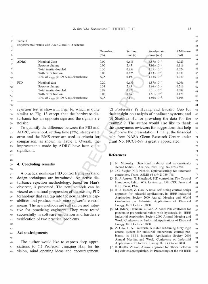
rejection test is shown in Fig. 16, which is quitesimilar to Fig. 13 except that the hardware dis-turbance has an opposite sign and the signals arenoisier.

To quantify the difference between the PID andADRC, overshoot, settling time (2%), steady-stateerror and the RMS error are used as criteria forcomparison, as shown in Table 1. Overall, theimprovements made by ADRC have been quitesignificant.

4. Concluding remarks

A practical nonlinear PID control framework anddesign techniques are introduced. An active dis-turbance rejection methodology, based on Han’sobserver, is presented. The new methods can beviewed as a natural progression of the existing PIDtechnology that can tap into the new hardware cap-abilities and produce much more powerful controlmeans. The new methods are still simple and intui-tive for practicing engineers. They were testedsuccessfully in software simulation and hardwareverification of two practical problems.

Acknowledgements

The author would like to express deep appre-ciations to (1) Professor Jingqing Han for hisvision, mind opening ideas and encouragement;

(2) Professors Yi Huang and Baozhu Guo fortheir insight on analysis of nonlinear systems; and(3) Shaohua Hu for providing the data for theexample 2. The author would also like to thankthe anonymous reviewers for suggestions that helpto improve the presentation. Finally, the financialhelp from NASA Glenn Research Center undergrant No. NCC3-699 is greatly appreciated.

References

[1] N. Minorsky, Directional stability and automatically

steered bodies, J. Am. Soc. Nav. Eng. 34 (1922) 280.

[2] J.G. Ziegler, N.B. Nichols, Optimal settings for automatic

controllers, Trans. ASME 64 (1942) 759–768.

[3] K. J. Astrom, T. Hagglund, PID control, in: The Control

Handbook, Editor W.S. Levine, pp. 198, CRC Press and

IEEE Press, 1996.

[4] R. J. Eucker, Z. Gao, A novel self-tuning control design

approach for industrial applications, in: IEEE Industrial

Application Society 2000 Annual Meeting and World

Conference on Industrial Applications of Electrical

Energy, 8–12 October 2000.

[5] M. (Marv) Hamdan, Z. Gao, A novel PID controller for

pneumatic proportional valves with hysteresis, in: IEEE

Industrial Application Society 2000 Annual Meeting and

World Conference on Industrial Applications of Electrical

Energy, 8–12 October 2000.

[6] Z. Gao, T. A. Trautzsch, A stable self-tuning fuzzy logic

control system for industrial temperature control pro-

blems, in: IEEE Industrial Application Society 2000

Annual Meeting and World Conference on Industrial

Applications of Electrical Energy, 8–12 October 2000.

[7] B. Boulter, Z. Gao, A novel approach for efficient self-tun-

ing web tension regulation, in: Proceedings of the 4th IEEE

Table 1

Experimental results with ADRC and PID schemes

Over-shoot

(%)

Settling

time (s)

Steady-state

error (rev)

RMS error

(rad)

ADRC Nominal Case 0.00 0.615 6.87�10�4 0.029

Setpoint change 0.00 2.45 3.80�10�3 0.116

Total inertia doubled 0.30 0.858 1.25�10�4 0.024

With extra friction 0.00 0.625 4.13�10�3 0.037

30% of Tmax (0.129 N.m) disturbance N/A 0.19 4.13�10�3 0.030

PID Nominal case 0.20 0.639 1.87�10�4 0.066

Setpoint change 0.34 2.43 1.86�10�2 0.216

Total inertia doubled 0.98 0.872 5.31�10�3 0.089

With extra friction 0.00 0.669 1.61�10�2 0.128

30% of Tmax (0.129 N.m) disturbance N/A 2.11 4.69�10�2. 0.196


1

2

3

4

5

6

7

8

9

10

11

12

13

14

15

16

17

18

19

20

21

22

23

24

25

26

27

28

29

30

31

32

33

34

35

36

37

38

39

40

41

42

43

44

45

46

47

48

49

50

51

52

53

54

55

56

57

58

59

60

61

62

63

64

65

66

67

68

69

70

71

72

73

74

75

76

77

78

79

80

81

82

83

84

85

86

87

88

89

90

91

92

93

94

95

96


UNCORREC

TEDPR

OOF


Conference on Control Applications; Real-Time Systems,

The Engineering of Complex Real-Time Computer Control

Systems, (special issue). The International Journal of Time-

Critical Computing Systems, 11(3) (November 1996).

[8] N. Dhayagude, Z. Gao, F. Mrad, Fuzzy logic control of

automated screw fastening, Journal Robotics and Com-

puter Aided Manufacturing 12 (3) (1996) 235–242.

[9] J. Han, Control theory: is it a theory of model or control?,

Systems Science and Mathematical Sciences 9 (4) (1989)

328–335, In Chinese.

[10] J. Han, W. Wang, Nonlinear tracking differentiator, Sys-

tems Science and Mathematical Sciences 14 (2) (1994)

177–183, In Chinese.

[11] J. Han, L. Yuan, The discrete form of the tracking differ-

entiator, Systems Science and Mathematical Sciences 19

(3) (1999) 268–273.

[12] J. Han, Nonlinear state error feedback control, Control

and Decision 10 (3) (1994) 221–225, In Chinese.

[13] J. Han, Nonlinear design methods for control systems, in:

The Proc. Of The 14th IFAC World Congress, Beijing, 1999.

[14] J. Han, Robustness of control system and the Godel’s

incomplete theorem, Control Theory and Its Applications

16(suppl.), (1999) 149-155, In Chinese.

[15] B. Guo, J. Han, A linear differentiator and application to

the online estimation of the frequency of a sinusoidal sig-

nal, in: Proceedings of the 2000 IEEE International Con-

ference on Control Applications, Anchorage, Alaska, 25–

27 September 2000.

[16] A. Levant, Robust exact differentiation via sliding mode

technique, Automatica 34 (3) (1998) 379–384.

[17] F. Jiang, A novel feedback control approach to a class of

anti-lock brake problems, Doctoral Dissertation, Depart-

ment of Electrical and Computer Engineering, Cleveland

State University, 1 May 2000.

[18] T. Stimac, Digital Control of a dc–dc Converter for Space

Applications, Department of Electrical and Computer

Engineering, Cleveland State University, December 2000.

[19] Y. Hou, Novel control approaches for web tension reg-

ulation, Doctoral Dissertation, Department of Electrical

and Computer Engineering, Cleveland State University,

May 2001.

[20] S. Hu, On high performance servo control solutions,

Doctoral Dissertation, Department of Electrical and

Computer Engineering, Cleveland State University, May

2001.

[21] Y. Hou, Z. Gao, F. Jiang, B. Boulter, Active disturbance

rejection control for web tension regulation, submitted for

publication.

[22] Z. Gao, S. Hu, F. Jiang, A novel motion control design

approach based on active disturbance rejection, submitted

for publication.

[23] G. Feng, L. Huang, A robust nonlinear controller for

induction motor, IFAC’99 G, 103–108.

Dr. Zhiqiang Gao is an Associ-

ate Professor of Electrical

Engineering at Cleveland State

University. He received a PhD

in Electrical Engineering from

University of Notre Dame in

1990. He is currently the direc-

tor of the Applied Control

Research Laboratory at CSU

and has collaborated exten-

sively with industry. He and his

group have developed a set of

innovative solutions including

nonl5inear control, fuzzy logic,

self-tuning, CAD software package etc. Applications of these

techniques can be found in many industry sectors such as

automotive, paper and pulp, manufacturing, medical instru-

mentation, and space electronics. Dr Gao also lectures broadly

in industry on advanced control topics.


1

2

3

4

5

6

7

8

9

10

11

12

13

14

15

16

17

18

19

20

21

22

23

24

25

26

27

28

29

30

31

32

33

34

35

36

37

38

39

40

41

42

43

44

45

46

47

48

49

50

51

52

53

54

55

56

57

58

59

60

61

62

63

64

65

66

67

68

69

70

71

72

73

74

75

76

77

78

79

80

81

82

83

84

85

86

87

88

89

90

91

92

93

94

95

96

From linear to nonlinear control means: a practical...

Documents

Transcript of From linear to nonlinear control means: a practical...