FROM KLEISLI CATEGORIES TO COMMUTATIVE … · c R. Furber and Bart Jacobs CC Creative Commons. 2 R....

Logical Methods in Computer ScienceVol. 11(1:5)2015, pp. 1–28www.lmcs-online.org

Submitted Feb. 21, 2014Published Jun. 10, 2015

FROM KLEISLI CATEGORIES TO COMMUTATIVE C∗-ALGEBRAS:

PROBABILISTIC GELFAND DUALITY

ROBERT FURBER AND BART JACOBS

Institute for Computing and Information Sciences (iCIS), Radboud University Nijmegen, TheNetherlands.e-mail address: {r.furber,bart}@cs.ru.nl

Abstract. C∗-algebras form rather general and rich mathematical structures that can

be studied with different morphisms (preserving multiplication, or not), and with differ-ent properties (commutative, or not). These various options can be used to incorporatevarious styles of computation (set-theoretic, probabilistic, quantum) inside categories ofC

∗-algebras. At first, this paper concentrates on the commutative case and shows thatthere are functors from several Kleisli categories, of monads that are relevant to model prob-abilistic computations, to categories of C∗-algebras. This yields a new probabilistic versionof Gelfand duality, involving the “Radon” monad on the category of compact Hausdorffspaces. We then show that the state space functor from C

∗-algebras to Eilenberg-Moorealgebras of the Radon monad is full and faithful. This allows us to obtain an appropriatelycommuting state-and-effect triangle for C∗-algebras.

1. Introduction

There are several notions of computation. We have the classical notion of computation,probabilistic computation, where a computer may make random choices, and quantumcomputation, which uses quantum mechanical interference and measurement. Normallywe would consider classical computation to be done on sets, probabilistic computation onspaces with a measure, and quantum computation on Hilbert spaces. We can instead usecategories with C∗-algebras as objects and a choice of either *-homomorphisms (called MIU-map below) or positive unital maps as the morphisms. We note at this point that positiveunital maps coincide with completely positive unital maps if either the domain or codomainof a map is a commutative C∗-algebra, but not in general. The general outline is representedin this table.

2012 ACM CCS: [Theory of computation]: Models of computation—Probabilistic computation /Quantum computation theory; Semantics and reasoning—Program semantics—Categorical semantics.

Key words and phrases: probabilistic computation, monad, functor, Kleisli, Gelfand, C*-algebra, commu-tative C*-algebra, compact Hausdorff space, convex, Radon measure, quantum computation.

LOGICAL METHODSl IN COMPUTER SCIENCE DOI:10.2168/LMCS-11(1:5)2015

c© R. Furber and Bart JacobsCC© Creative Commons

http://creativecommons.org/about/licenses

2 R. FURBER AND BART JACOBS

set-theoretic probabilistic quantum

C∗-algebras commutative commutative non-commutative

maps preservemultiplicationinvolution

unit

positivityunit

positivityunit

maps abbreviation MIU PU PU

While the quantum case is an important source of motivation, we will deal more with theclassical and probabilistic cases in this article. In particular, we will relate the alterna-tive method of representing probabilistic computation, using monads, to the C∗-algebraicapproach.

In recent years the methods and tools of category theory have been applied to Hilbertspaces — see e.g. [1] and the references there — and also to C∗-algebras, see for instance [32,29]. In this paper we show that clearly distinguishing different types of homomorphisms ofC∗-algebras already brings quite some clarity. Moreover, we demonstrate the relevance ofmonads (and their Kleisli and Eilenberg-Moore categories) in this field. The aforementionedpaper [32] concerns itself with only the *-homomorphisms (i.e. with the MIU-maps in ourterminology).

The main results of the paper can be summarised as follows. The well-known finite(‘baby’) version of Gelfand duality involves an equivalence between on the one hand thecategory of finite sets (and all functions between them), and on the other hand the op-posite of the category of finite-dimensional commutative C∗-algebras with MIU-maps (*-homomorphisms) between them. Diagrammatically:

FinSets≃ //

(

FdCCstarMIU

)op

Our first observation is that if we generalise from MIU to PU (positive unital) maps we getan equivalence:

KℓN(D)≃ //

(

FdCCstarPU)op

whereD is the distribution monad on Sets, and KℓN(D) is the Kleisli category of this monad,but with objects restricted to natural numbers. This shows that the category FdCCstarPUis the Lawvere theory of the distribution monad. Details are in Section 4.

The main contribution of the paper lies in a generalisation of the latter equivalencebeyond the finite case, which can be summarised in a diagram:

CH≃

Gelfand//

��

R

%% (

CCstarMIU

)op

� _

��Kℓ(R)

≃new

//

⊣

OO

(

CCstarPU)op

(1.1)

At the top of this diagram we have the classical Gelfand duality between the categoryCH of compact Hausdorff spaces and the (opposite of the) category of commutative C∗-algebras with MIU-maps. Again, the generalisation to the computationally more interestingPU-maps involves a duality with a Kleisli category, namely the Kleisli category Kℓ(R) ofwhat we call the Radon monad R on compact Hausdorff spaces. Elements of R(X) can be

PROBABILISTIC GELFAND DUALITY 3

described as so-called Radon probability measures, also known as inner regular probabilitymeasures (see [33]).

In the end, in Diagram (6.1) we show how the Kleisli category of the Radon monadgives rise to a ‘state-and-effect’ triangle that combines Kleisli computations for the Radonmonad and their associated predicate transformers and state transformers. These predicateand state transformers correspond to the Heisenberg and Schrodinger picture, respectively.

Incidentally, the adjunction on the left in Diagram (1.1) can be transferred to the right,and then yields a right adjoint to the inclusion CCstarMIU → CCstarPU. In [40] it isshown that such a right adjoint also exists in the general non-commutative case.

Giry [14, I.4] described how we can consider a stochastic process as being a diagramin the Kleisli category of the Giry monad on measure spaces. By using the Radon monadR on compact spaces instead, we can get a different category of stochastic processes oncompact spaces as diagrams in the (opposite of the) category of commutative C∗-algebraswith PU-maps. This allows the quantum generalization to taking diagrams in the categoryof non-commutative C∗-algebras, or by considering diagrams in the category EM(R) ofEilenberg-Moore algebras of the Radon monad R, in which the category of C∗-algebrasfaithfully embeds. The relationship to quantum computation is that B(H), the algebraof all bounded operators on a Hilbert space H, is a C∗-algebra, and for every C∗-algebraA, there is a Hilbert space H such that A is isomorphic to a norm-closed *-subalgebraof B(H). Unitary maps U : H → H define MIU maps a 7→ U∗aU : B(H) → B(H). Thecategory of C∗-algebras allows us to represent measurement with maps from a commutativeC∗-algebra to B(H). We can also represent composite systems that are partly quantumand partly classical. Girard also used certain special C∗-algebras, von Neumann algebras,for his Geometry of Interaction [13].

2. Preliminaries on C∗-algebras

We write Vect = VectC for the category of vector spaces over the complex numbers C. Thiscategory has direct product V ⊕W , forming a biproduct (both a product and a coproduct)and tensors V ⊗W , which distribute over ⊕. The tensor unit is the space C of complexnumbers. The unit for ⊕ is the singleton (null) space 0. We write V for the vector spacewith the same vectors/elements as V , but with conjugate scalar product: z •V v = z •V v.This makes Vect an involutive category, see [19].

A *-algebra is an involutive monoid A in the category Vect. Thus, A is itself a vectorspace, carries a multiplication · : A⊗A→ A, linear in each argument, and has a unit 1 ∈ A.Moreover, there is an involution map (−)∗ : A→ A, preserving 0 and + and satisfying:

1∗ = 1 (x · y)∗ = y∗ · x∗ x∗∗ = x (z • x)∗ = z • x∗.

Here we have written a fat dot • for scalar multiplication, to distinguish it from the algebra’smultiplication ·. For z = a + bi ∈ C we have the conjugate z = a − bi. Often we omit themultiplication dot · and simply write xy for x · y. Similarly, the scalar multiplication • isoften omitted. We then rely on the context to distinguish the two multiplications.

A C∗-algebra is a *-algebra A with a norm ‖ − ‖ : A → R≥0 in which it is complete,satisfying the conditions ‖x‖ = 0 iff x = 0 and:

‖x+ y‖ ≤ ‖x‖+ ‖y‖ ‖z • x‖ = |z| · ‖x‖

‖x · y‖ ≤ ‖x‖ · ‖y‖ ‖x∗ · x‖ = ‖x‖2.


The last equation ‖x∗ · x‖ = ‖x‖2, is the C∗-identity and distinguishes C∗-algebras fromBanach *-algebras. We remark at this point that a Banach *-algebra admits at most onenorm satisfying the C∗-identity. The reason for this is that the spectral radius r(x) isdefinable in terms of the ring structure of the algebra, and for self-adjoint elements r(x) =‖x‖ [24, Proposition 4.1.1 (a)]. If x is an arbitrary element, x∗ ·x is self-adjoint, so r(x∗ ·x) =‖x∗ · x‖ = ‖x‖2. In the current setting, each C∗-algebra is unital, i.e. has a (multiplicative)unit 1. A consequence of the axioms above is that ‖1‖ = 1 unless the C∗-algebra is theunique one in which 0 = 1. A C∗-algebra is called commutative if its multiplication iscommutative, and finite-dimensional is it has finite dimension when considered as a vectorspace.

An element x in a C∗-algebra A is called positive if it can be written in the formx = y∗ · y. We write A+ ⊆ A for the subset of positive elements in A. This subset is acone, which is to say it is closed under addition and scalar multiplication with positive realnumbers. The multiplication x · y of two positive elements need not be positive in general(think of matrices). The square x2 = x · x of a self-adjoint element x = x∗, however, isobviously positive. In a commutative C∗-algebra the positive elements are closed undermultiplication. A cone A+ in a vector space defines a partial order as follows.

x ≤ y ⇐⇒ y − x ∈ A+. (2.1)

This is defines an order on every C∗-algebra.There are mainly two options when it comes to maps between C∗-algebras. The differ-

ence between them plays an important role in this paper.

Definition 2.1. We define two categories CstarMIU and CstarPU with C∗-algebras asobjects, but with different morphisms.

(1) A morphism f : A → B in CstarMIU is a linear map preserving multiplication (M),involution (I), and unit (U). Explicitly, this means for all x, y ∈ A,

f(x · y) = f(x) · f(y) f(x∗) = f(x)∗ f(1) = 1.

Often such “MIU” maps are called *-homomorphisms.(2) A morphism f : A → B in CstarPU is a linear map that preserves positive elements

and the unit. This means that f restricts to a function A+ → B+. Alternatively, foreach x ∈ A there is an y ∈ B with f(x∗x) = y∗y.

For bothX = MIU andX = PU there are obvious full subcategories of commutative and/orfinite-dimensional C∗-algebras, as described in:

CCstarX � x

++❱❱❱❱❱❱❱

❱❱

FdCCstarX

%�

33❣❣❣❣❣❣❣❣❣� y

++❲❲❲❲❲❲❲

❲CstarX

FdCstarX

&�

33❤❤❤❤❤❤❤❤

Clearly, each “MIU” map is also a “PU” map, so that we have inclusions CstarMIU →CstarPU, also for the various subcategories. A map that preserves positive elements iscalled positive itself; and a unit preserving map is called unital. Positive unital maps arethe natural notion of morphism between order unit spaces and Riesz spaces.

For a category B one often writesB(X,Y ) or Hom(X,Y ) for the “homset” of morphismsX → Y in B. For C∗-algebras A,B we write HomMIU(A,B) = CstarMIU(A,B) and


HomPU(A,B) = CstarPU(A,B) for the homsets of MIU- and PU-maps. For the special casewhereB is the algebra C of complex numbers we define sets of “states” and of “multiplicativestates” as:

Stat(A) = HomPU(A,C) and MStat(A) = HomMIU(A,C).

There is also the commonly used notion of completely positive maps, which is a strongercondition than positivity but weaker than being MIU. These maps are important whendefining the tensor of C∗-algebras as a functor, as the tensor of positive maps need not bepositive. They are also widely considered to represent the physically realizable transforma-tions. Positive, but non-completely positive maps of C∗-algebras also have their uses, asentanglement witnesses for example [17, theorem 2]. Since we mainly consider the commu-tative case, where positive and completely positive coincide, we do not consider the categoryof C∗-algebras with completely positive maps any further in this paper. However, since acompletely positive unital map is what is known as a channel in quantum information, thentheorem 5.1 shows that every channel in Mislove’s sense [30] is a channel in this sense.

We collect some basic (standard) properties of PU-morphisms between C∗-algebras (seee.g. [35, 5]).

Lemma 2.2. A PU-map, i.e. a morphism in the category CstarPU, commutes with invo-lution (−)∗, and preserves the partial order ≤ given by (2.1).

Moreover, a PU-map f satisfies ‖f(x)‖ ≤ 4‖x‖, so that ‖f(x) − f(y)‖ ≤ 4‖x − y‖,making f continuous.

Proof. An element x is called self-adjoint if x∗ = x. Each self-adjoint x can be writtenuniquely as a difference x = xp − xn of positive elements xp, xn, with xpxn = xnxp = 0and ‖xp‖, ‖xn‖ ≤ ‖x‖, see [24, Proposition 4.2.3 (iii)]; as a result f(x∗) = f(x) = f(x)∗,for a PU-map f . Next, an arbitrary element y can be written uniquely as y = yr + iyifor self-adjoint elements yr = 1

2(y + y∗), yi =12i (y − y∗), so that ‖yr‖, ‖yi‖ ≤ ‖y‖. Then

f(y∗) = f(y)∗. Preservation of the order is trivial.For positive x we have x ≤ ‖x‖ • 1, and thus f(x) ≤ ‖x‖ • 1, which gives ‖f(x)‖ ≤ ‖x‖.

An arbitrary element x can be written as linear combination of four positive elements xi,as in x = x1−x2+ ix3− ix4, with ‖xi‖ ≤ ‖x‖. Finally, ‖f(x)‖ = ‖f(x1)− f(x2)+ if(x3)−if(x4)‖ ≤

∑

i ‖f(xi)‖ ≤∑

i ‖xi‖ ≤ 4‖x‖.

In fact, it can be shown that ‖f(x)‖ ≤ ‖x‖ for all x, not just positive x, reducing theconstant 4 in the inequality above to 1 (see [34, corollary 1]). But this sharpening is notneeded here.

We next recall two famous adjunctions involving compact Hausdorff spaces. The firstone is due to Manes [28] and describes compact Hausdorff spaces as monadic over Sets,via the ultrafilter monad. The second one is known as Gelfand duality, relating compactHausdorff spaces and commutative C∗-algebras. Notice that this result involves the “MIU”maps.

Theorem 2.3. Let CH be the category of compact Hausdorff spaces, with continuous mapsbetween them. There are two fundamental adjunctions:

CH

forget

��

CH

C

��⊣ ≃

Sets

U

EE

(CCstarMIU)op

MStat

YY


On the left the functor U sends a set X to the ultrafilters on the powerset P(X). And on theright the equivalence of categories is given by sending a compact Hausdorff space X to thecommutative C∗-algebra C(X) = Cont(X,C) of continuous functions X → C. The “weak-*topology” on states will be discussed below.

The multiplicative states on a commutative C∗-algebra can equivalently be describedas maximal ideals, or also as so-called pure states (see below).

Corollary 2.4. For each finite-dimensional commutative C∗-algebra A there is an n ∈ N

with A ∼= Cn in FdCCstarMIU.

Proof. By the previous theorem there is a compact Hausdorff space X such that A is MIU-isomorphic to the algebra of continuous maps X → C. This X must be finite, and since afinite Hausdorff space is discrete, all maps X → C are continuous. Let n ∈ N be the numberof elements in X; then we have an isomorphism A ∼= C

n.

As we can already see in the above theorem, it is the opposite of a category of C∗-algebras that provides the most natural setting for computations. This is in line with whatis often called the Heisenberg picture. In a logical setting it corresponds to computation ofweakest preconditions, going backwards. The situation may be compared to the category ofcomplete Heyting algebras, which is most usefully known in opposite form, as the categoryof locales, see [23].

The set of states Stat(A) = HomPU(A,C) now can be equipped with the weak-*topology, defined as the coarsest (smallest) topology in which all evaluation maps evx =λs. s(x) : HomPU(A,C) → C, for x ∈ A, are continuous. We introduce the categoryCCLcvx, which first appeared in [39], in order to extend Stat to a functor.

The category CCLcvx has as its objects compact convex subsets of (Hausdorff) locallyconvex vector spaces. More accurately, the objects are pairs (V,X) where V is a (Hausdorff)locally convex space, and X is a compact convex subset of V . The maps (V,X) → (W,Y )are continuous, affine maps X → Y . Note that if (V,X) and (W,Y ) are isomorphic, whileX is necessarily homeomorphic to Y , V need not bear any particular relation to W at all.We can see CCLcvx forms a category, as identity maps are affine and continuous and bothof these attributes of a map are preserved under composition. We remark at this point thatwe have a forgetful functor U : CCLcvx → CH, taking the underlying compact Hausdorffspace of X.

Proposition 2.5. For each C∗-algebra A, the set of states Stat(A) = HomPU(A,C) isconvex, and is a compact Hausdorff subspace of the dual space of A given the weak-* topology.Each PU-map f : A→ B yields an affine continuous function Stat(f) = (−) ◦ f : Stat(B) →Stat(A). This defines a functor Stat : (CstarPU)

op → CCLcvx.

We recall that a function (between convex sets) is called affine if it preserves convexsums. We will see shortly that such affine maps are homomorphisms of Eilenberg-Moorealgebras for the distribution monad D.

Proof. For each finite collection hi ∈ HomPU(A,C) with ri ∈ [0, 1] satisfying∑

i ri = 1,the function h =

∑

i rihi is again a state. Moreover, such convex sums are preserved byprecomposition, making the maps (−) ◦ f affine.

The fact that the dual space of A, given the weak-* topology, is a locally convex spaceis standard, and only uses that A is a Banach space [7, Example 1.8]. This implies that thespace of states is Hausdorff. The space of states is closed since because the positive cone in


a C∗-algebra is closed [24, Proposition 2.4.5 (i)][8, Proposition 1.6.1] and the set of linearfunctionals such that φ(1) = 1 is weak-* closed, and the set of states is the intersection ofthe two. The space of states is also bounded as each state has norm 1. Therefore the statespace is a closed and bounded and hence compact by the Banach-Alaoglu Theorem.

Precomposition (−) ◦ f is continuous, since for x ∈ A and U ⊆ C open we get an open

subset(

(−) ◦ f)−1

(ev−1x (U)) = {h | evx(h ◦ f) ∈ U} = ev−1

f(x)(U).

Precomposition with the identity map gives the same state again, so Stat preservesidentity maps. Since composition of PU-maps is associative, Stat preserves composition,and hence is a functor.

2.1. Effect modules. Effect algebras have been introduced in mathematical physics [10],in the investigation of quantum probability, see [9] for an overview. An effect algebra is apartial commutative monoid (M, 0,>) with an orthocomplement (−)⊥. One writes x ⊥ y ifx> y is defined. The formulation of the commutativity and associativity requirements is abit involved, but essentially straightforward. The orthocomplement satisfies x⊥⊥ = x andx > x⊥ = 1, where 1 = 0⊥. There is always a partial order, given by x ≤ y iff x > z = y,for some z. The main example is the unit interval [0, 1] ⊆ R, where addition + is obviouslypartial, commutative, associative, and has 0 as unit; moreover, the orthocomplement isr⊥ = 1− r. We write EA for the category of effect algebras, with morphism preserving >

and 1 — and thus all other structure.For each set X, the set [0, 1]X of fuzzy predicates onX is an effect algebra, via pointwise

operations. Each Boolean algebra B is an effect algebra with x ⊥ y iff x ∧ y = ⊥; thenx > y = x ∨ y. In a quantum setting, the main example is the set of effects Ef(H) ={E : H → H | 0 ≤ E ≤ I} on a Hilbert space H, see e.g. [9, 16].

An effect module is an “effect” version of a vector space. It involves an effect algebraM with a scalar multiplication s • x ∈ M , where s ∈ [0, 1] and x ∈ M . This scalarmultiplication is required to be a suitable homomorphism in each variable separately. Thealgebras [0, 1]X and Ef(H) are clearly such effect modules. Maps in EMod are EA mapsthat are additionally required to commute with scalar multiplication.

For a C∗-algebra A the subset A+ → A of positive elements carries a partial order ≤defined on self-adjoint elements in (2.1). We write [0, 1]A ⊆ A+ ⊆ A for the subset of positiveelements below the unit. The elements in [0, 1]A will be called effects (or sometimes also:predicates). For instance, for the C∗-algebra B(H) of bounded operators on a Hilbert spaceH the unit interval [0, 1]B(H) ⊆ B(H) contains the effects Ef(H) = {A ∈ B(H) | 0 ≤ A ≤ id}on H.

We claim that [0, 1]A is an effect algebra and carries a [0, 1] ⊆ R scalar multiplication,thus making it an effect module.

• Since A with 0,+ is a partially ordered Abelian group, [0, 1]A is a so-called interval effectalgebra, with x ⊥ y iff x+ y ≤ 1, and in that case x> y = x+ y. The orthocomplementx⊥ is given by 1− x.

• For r ∈ [0, 1] and x ∈ [0, 1]A the scalar multiplications rx and (1− r)x are positive, andtheir sum is x ≤ 1. Hence rx ≤ 1 and thus rx ∈ [0, 1]A.

Each PU-map of C∗-algebras f : A → B preserves ≤ and thus restricts to [0, 1]A → [0, 1]B .This restriction is a map of effect modules. Hence we get a “predicate” functor CstarPU →EMod.


Lemma 2.6. The functor [0, 1](−) : CstarPU → EMod is full and faithful.

Proof. Any PU-map f : A → B is completely determined (and defined by) its action on[0, 1]A: for a non-zero positive element x ∈ A we use x ≤ ‖x‖ 1 and thus 1

‖x‖ x ∈ [0, 1]A to

see that f(x) = ‖x‖ f( 1‖x‖ x). An arbitrary element y ∈ A can be written uniquely as linear

sum of four positive elements (see Lemma 2.2), determining f(y).

The (finite, discrete probability) distribution monad D : Sets → Sets sends a set X tothe set D(X) = {ϕ : X → [0, 1] | supp(ϕ) is finite, and

∑

x ϕ(x) = 1}, where supp(ϕ) ={x | ϕ(x) 6= 0}. Such an element ϕ ∈ D(X) may be identified with a finite, formal convexsum

∑

i rixi with xi ∈ X and ri ∈ [0, 1] satisfying∑

i ri = 1. The unit η : X → D(X) andmultiplication µ : D2(X) → D(X) of this monad are given by singleton/Dirac convex sumand by matrix multiplication:

η(x) = 1x µ(Φ)(x) =∑

ϕ Φ(ϕ) · ϕ(x).

A convex set is an Eilenberg-Moore algebra of this monad: it consists of a carrier set X inwhich actual sums

∑

i rixi ∈ X exist for all convex combinations. We writeConv = EM(D)for the category of convex sets, with “affine” functions preserving convex sums.

Effect modules and convex sets are related via a basic adjunction [22], obtained by“homming into [0, 1]”, as in:

EModop

EMod(−,[0,1]),,

⊤ Conv

Conv(−,[0,1])

mm (2.2)

3. Set-theoretic computations in C∗-algebras

For a set X, a function f : X → C is called bounded if |f(x)| ≤ s, for some s ∈ R≥0. Wewrite ℓ∞(X) for the set of such bounded functions. Notice that if X is finite, any functionX → C is bounded, so that ℓ∞(X) = C

X .Each ℓ∞(X) is a commutative C∗-algebra, with pointwise addition, multiplication and

involution, and with the uniform/supremum norm:

‖f‖∞ = inf{s ∈ R≥0 | ∀x. |f(x)| ≤ s}.

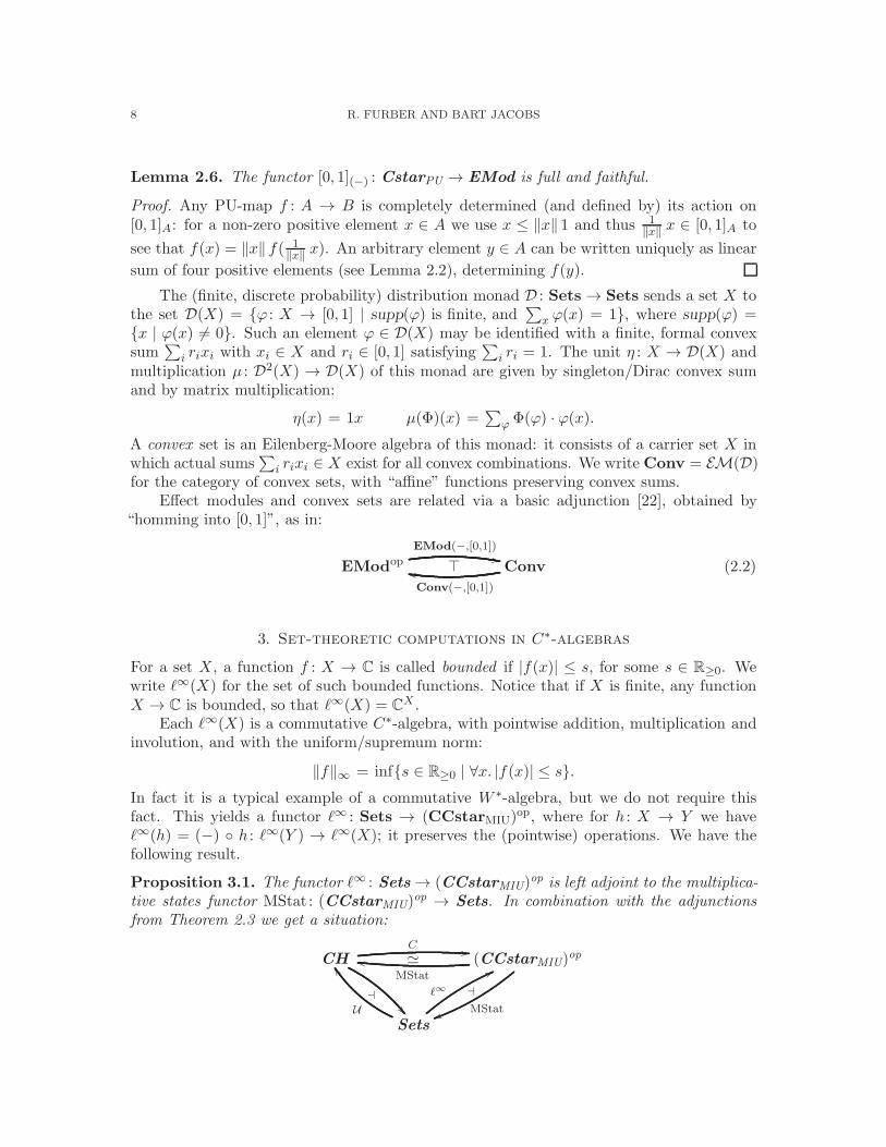
In fact it is a typical example of a commutative W ∗-algebra, but we do not require thisfact. This yields a functor ℓ∞ : Sets → (CCstarMIU)

op, where for h : X → Y we haveℓ∞(h) = (−) ◦ h : ℓ∞(Y ) → ℓ∞(X); it preserves the (pointwise) operations. We have thefollowing result.

Proposition 3.1. The functor ℓ∞ : Sets → (CCstarMIU)op is left adjoint to the multiplica-

tive states functor MStat : (CCstarMIU)op → Sets. In combination with the adjunctions

from Theorem 2.3 we get a situation:

CH

⊣

��

C ..≃ (CCstarMIU)

op

MStat

mm

⊣

MStatuuSets

U

ZZ

ℓ∞

66


By composition and uniqueness of adjoints we get:

C ◦ U ∼= ℓ∞ and also MStat ◦ ℓ∞ ∼= U .

Proof. Note that MStat is used in two different senses in the above diagram, in one casewith a compact Hausdorff topology, and in the other case simply as a set. The adjunctioninvolving ℓ∞ and MStat is for MStat as a set. We show this adjunction using the universalproperty of the unit of an adjunction. We define the unit ηX : X → MStat(ℓ∞(X)), whereX ∈ Sets, as

ηX(x)(a) = a(x),

where a ∈ ℓ∞(X). Then ηX(x) is a multiplicative state on ℓ∞(X) because the vectorspace structure, multiplication and multiplicative unit are defined pointwise. To showthe naturality square for η commutes, we must show that for all f : X → Y in Sets,MStat(ℓ∞(f)) ◦ ηX = ηY ◦ f . If we take x ∈ X and b ∈ ℓ∞(Y ), we have:

(

MStat(ℓ∞(f)) ◦ ηX)

(x)(b) = MStat(ℓ∞(f))(ηX(x))(b)

= (ηX(x) ◦ ℓ∞(f))(b)

= ηX(x)(ℓ∞(f)(b))

= ηX(x)(b ◦ f)

= b(f(x))

= ηY (f(x))(b)

= (ηY ◦ f)(x)(b).

We now show this natural transformation satisfies the universal property making it theunit of the adjunction. Let X ∈ Sets, B ∈ CCstarMIU and f : X → MStat(B). Defineg : B → ℓ∞(X) as g(b)(x) = f(x)(b). We must show that g(b) is an element of ℓ∞(X),i.e. that it is bounded. For all x ∈ X, f(x) is a multiplicative state, hence a state, so by[8, Proposition 2.1.4] we have ‖f(x)‖ = 1, and so |g(b)(x) = |f(x)(b)| ≤ ‖f(x)‖‖b‖ = ‖b‖.Therefore ‖b‖ is a bound for g(b), showing that it is a bounded function. The fact that g isan MIU map is easily deduced from the fact that f(x) is a multiplicative state for all x (itwould fail if f(x) were only a state).

We must now show that

XηX //

f ((◗◗◗◗

◗◗◗◗

◗◗◗◗

◗◗◗ MStat(ℓ∞(X))

MStat(g)��

MStat(B)

commutes. Taking x ∈ X and b ∈ B, we see

MStat(g)(ηX (x))(b) = (ηX(x) ◦ g)(b)

= ηX(x)(g(b))

= g(b)(x)

= f(x)(b),

and hence the unit diagram commutes.To show the uniqueness of g, suppose there were h : B → ℓ∞(X) that also made the unit

diagram commute. By evaluating MStat(h)(ηX (x))(b) we would obtain g(b)(x) = h(b)(x).


Since g(b) and h(b) are elements of ℓ∞(X) and hence functions, this implies g(b) = h(b)by extensionality, and we can then conclude that g = h, as required. We have now shownthat ℓ∞ is a left adjoint to MStat. The other two adjunctions are simply the Stone-Cechcompactification of a set and Gelfand duality (which is even an equivalence).

Since the triangle consisting of MStat, in both forms, and the forgetful functor CH →Sets commutes, the triangle for ℓ∞,U and C commutes up to isomorphism, i.e. ℓ∞ ∼= C ◦ Uby uniqueness of adjoints.

When we restrict to the full subcategory FinSets → Sets of finite sets we obtain afunctor ℓ∞ = C

(−) : FinSets → (FdCCstarMIU)op. The next result is then a well-known

special case of Gelfand duality (Theorem 2.3). We elaborate the proof in some detail becauseit is important to see where the preservation of multiplication plays a role.

Proposition 3.2. The functor C(−) : FinSets → (FdCCstarMIU)

op is an equivalence ofcategories.

Proof. It is easy to see that the functor C(−) is faithful. The crucial part is to see that

it is full. So assume we have two finite sets, seen as natural numbers n,m, and a MIU-homomorphism h : Cm → C

n. For j ∈ m, let |j 〉 ∈ Cm be the standard base vector with 1

at the j-th position and 0 elsewhere. Since this |j 〉 is positive, so is h(|j 〉), and thus we maywrite it as h(|j 〉) = (r1j , . . . , rnj), with rij ∈ R≥0. Because |j 〉 · |j 〉 = |j 〉, and h preservesmultiplication, we get h(|j 〉) · h(|j 〉) = h(|j 〉), and thus r2ij = rij . This means rij ∈ {0, 1},so that h is a (binary) Boolean matrix. But h is also unital, and so:

1 = h(1) = h(|1〉 + · · · + |m〉) = h(|1〉) + · · ·+ h(|m〉). (3.1)

For each i ∈ n there is thus precisely one j ∈ m with rij = 1 — so that h is a “functional”

Boolean matrix. This yields the required function f : n→ m with Cf = h.

Corollary 2.4 says that the functor C(−) : FinSets → (FdCCstarMIU)op is essentially

surjective on objects, and thus an equivalence.

This proof demonstrates that preservation of multiplication, as required for “MIU”maps, is a rather strong condition. We make this more explicit.

Corollary 3.3. For n ∈ N we have MStat(Cn) ∼= n.

Proof. By identifying n ∈ N with the n-element set n = {0, 1, . . . , n− 1} ∈ FinSets, we getby Proposition 3.2, MStat(Cn) = HomMIU(C

n,C) ∼= FinSets(1, n) ∼= n.

4. Discrete probabilistic computations in C∗-algebras

We turn to probabilistic computations and will see that we remain in the world of commu-tative C∗-algebras, but with PU-maps (positive unital) instead of MIU-maps. Recall thatthe set of states Stat(A) of a C∗-algebra A contains the PU-maps A→ C.

We summarize here the definition of the expectation monad given in [21]. If [0, 1]X

is the effect module of functions from X to [0, 1] with pointwise operations, E(X) =EMod([0, 1]X , [0, 1]). The unit ηX : X → E(X) is evaluation, defined as ηX(x)(f) = f(x)

for f ∈ [0, 1]X . The multiplication µX : E2(X) → E(X) is defined for h ∈ [0, 1]E(X) → [0, 1],p ∈ [0, 1]X as

µX(h)(p) = h(

λk ∈ E(X). k(p))

.


Lemma 4.1. Sending a set X to the set of states of the C∗-algebra ℓ∞(X) yields the(underlying functor of the) expectation monad E from [21]: the mapping X 7→ Stat(ℓ∞(X))is isomorphic to the expectation monad E : Sets → Sets, defined in [21] via effect modulehomomorphisms: E(X) = EMod

(

[0, 1]X , [0, 1])

.As a result, Stat(Cn) ∼= D(n), for n ∈ N, where D(n) is the standard n-simplex.

Proof. The predicate/effect functor [0, 1](−) : CstarPU → EMod is full and faithful byLemma 2.6, and so:

Stat(ℓ∞(X)) = HomPU

(

ℓ∞(X),C)

∼= EMod(

[0, 1]ℓ∞(X), [0, 1]C)

= EMod(

[0, 1]X , [0, 1])

= E(X).

The isomorphism α : HomPU(Cn,C)

∼=−→ D(n) follows because the expectation and distribu-tion monad coincide on finite sets, see [21]. Explicitly, it is given by α(h) = λi ∈ n. h(|i〉)and α−1(ϕ)(v) =

∑

i ϕ(i) · v(i).

The unit η and multiplication µ structure on E(X) ∼= HomPU(ℓ∞(X),C) is very much

like for “continuation” or “double dual” monads, see [26, 31, 18], with:

Xη // HomPU(ℓ

∞(X),C) HomPU

(

ℓ∞(

HomPU(CX ,C)

)

,C)

µ // HomPU(ℓ∞(X),C)

x✤ // λv. v(x) g

✤ // λv. g(

λh. h(v))

.

For an arbitrary monad T = (T, η, µ) on a category B we write Kℓ(T ) for the Kleislicategory of T . Its objects are the same as those of B, but its maps X → Y are the mapsX → T (Y ) in B. The unit η : X → T (X) is the identity map X → X in Kℓ(T ); andcomposition of f : X → Y and g : Y → Z in Kℓ(T ) is given by g ⊙ f = µ ◦ T (g) ◦ f .Maps in such a Kleisli category are understood as computations with outcomes of type T ,see [31]. For a monad T : Sets → Sets we write KℓN(T ) → Kℓ(T ) for the full subcategorywith numbers n ∈ N as objects, considered as n-element sets.

Proposition 4.2. The expectation monad E(X) ∼= HomPU(ℓ∞(X),C) gives rise to a full

and faithful functor:

Kℓ(E)CE // (CCstarPU)

op

X✤ // ℓ∞(X)

(

Xf→ E(Y )

)

✤ // λv ∈ ℓ∞(Y ). λx ∈ X. f(x)(v).

(4.1)

Proof. First we need to see that CE(f) is well-defined: the function CE(f)(v) : X → C mustbe bounded. We can apply Lemma 2.2 to the function f(x) ∈ HomPU(ℓ

∞(Y ),C); it yields‖f(x)(v)‖ ≤ 4‖v‖. This holds for each x ∈ X, so that |CE (f)(v)(x)| = |f(x)(v)| is boundedby 4‖v‖. Next, the map CE(f) is a PU-map of C∗-algebras via the pointwise definitions ofthe relevant constructions.


We check that CE preserves (Kleisli) identities and composition:

CE(id)(v)(x) = CE(η)(v)(x)

= η(x)(v)

= v(x)

CE(g ⊙ f)(v)(x) = (g ⊙ f)(x)(v)

= µ(

E(g)(f(x)))

(v)

= E(g)(f(x))(

λw.w(v))

= f(x)(

(λw.w(v)) ◦ g)

= f(x)(

λy. g(y)(v))

= f(x)(

CE(g)(v))

= CE(f)(

CE(g)(v))

(x)

=(

CE(f) ◦ CE(g))

(v)(x).

Further, CE is obviously faithful, and it is full since for h : ℓ∞(Y ) → ℓ∞(X) in CCstarPU wecan define f : X → HomPU(ℓ

∞(Y ),C) by f(x)(v) = h(v)(x). Then each f(x) is a PU-mapof C∗-algebras.

We turn to the finite case, like in the previous section. We do so by considering theKleisli category KℓN(E) obtained by restricting to objects n ∈ N. Since the expectationmonad E and the distribution monad D coincide on finite sets, we have KℓN(E) ∼= KℓN(D).Maps n→ m in this category are probabilistic transition matrices n→ D(m). This categoryhas been investigated also in [12]. The following equivalence is known, see e.g. [27], althoughpossibly not in this categorical form.

Proposition 4.3. The functor CE from (4.1) restricts in the finite case to an equivalenceof categories:

KℓN(D)CD

≃// (FdCCstarPU)

op (4.2)

It is given by CD(n) = Cn and CD

(

nf→ D(m)

)

= λv ∈ Cm. λi ∈ n.

∑

j∈mf(i)(j) · v(j).

This equivalence (4.2) may be read as: the category FdCCstarPU of finite-dimensionalcommutative C∗-algebras, with positive unital maps, is the Lawvere theory of the distribu-tion monad D.

Proof. Fullness and faithfulness of the functor CD follow from Proposition 4.2, using the iso-morphism HomPU(C

n,C) ∼= D(n) from Lemma 4.1. This functor CD is essentially surjectiveon objects by Corollary 2.4, using the fact that a MIU-map is a PU-map.

5. Continuous probabilistic computations

The question arises if the full and faithful functor Kℓ(E) → (CCstarPU)op from Proposi-

tion 4.2 can be turned into an equivalence of categories, but not just for the finite case likein Proposition 4.3. In order to make this work we have to lift the expectation monad E on


Sets to the category CH of compact Hausdorff spaces. As lifting we use what we call theRadon monad R, defined on X ∈ CH as:

R(X) = Stat(C(X)) = HomPU

(

C(X), C)

, (5.1)

where, as usual, C(X) = {f : X → C | f is continuous}; notice that the functions f ∈ C(X)are automatically bounded, since X is compact. We have implicitly applied the forgetfulfunctor fromCCLcvx → CH to make R into an endofunctor ofCH. The elements ofR(X)are related to measures in the following way. If µ is a probability measure on the Borel sets ofX, integration of continuous functions with respect to µ gives a function

∫

X−dµ ∈ R(X).

A Radon probability measure, or an inner regular probability measure, is one such thatµ(S) = supK⊆S µ(K) where K ranges over compact sets. The map from measures toelements of R(X) is a bijection [33, Thm. 2.14], and accordingly we shall sometimes refer toelements of R(X) as measures. Therefore the Radon monad can be considered as a variantof the Giry monad. In fact there are two Giry monads, one on measurable spaces and oneon Polish spaces. The Radon monad differs from the Giry monad on measurable spaces inthat it uses the topology of a space, and that in the case of a space that is not a standardBorel space there can be non-Radon measures [11, 434K (d), page 192] [15, §53.10, page231]. The Radon monad differs from the Giry monad on Polish spaces essentially only inthe choice of spaces, and on compact Polish spaces they agree, as the topology Giry usedis the same as the weak-* topology, and Polish spaces do not admit any non-Radon Borelprobability measures.[6, Theorems 1.1 and 1.4].

This Radon monad R is not new: we shall see later that it occurs in [39, Theorem 3]as the monad of an adjunction (“probability measure” is used to mean “Radon probabilitymeasure” in that article). It has been used more recently in [30]. However, our dualityresult below — Theorem 5.1 — is not known in the literature.

From Proposition 2.5 it is immediate that R(X) is again a compact Hausdorff space.The unit η : X → R(X) and multiplication µ : R2(X) → R(X) are defined as for theexpectation monad, namely as η(x)(v) = v(x) and µ(g)(v) = g

(

λh. h(v))

. We check that ηis continuous. Recall from the proof of Proposition 2.5 that a basic open in R(X) is of theform ev−1

s (U) = {h ∈ R(X) | h(s) ∈ U}, where s ∈ C(X) and U ⊆ C is open. Then:

η−1(

ev−1s (U)

)

= {x ∈ X | η(x)(s) ∈ U} = {x ∈ X | s(x) ∈ U} = s−1(U).

The latter is an open subset of X since s : X → C is a continuous function.We are now ready to state our main, new duality result. It may be understood as a

probabilistic version of Gelfand duality, for commutative C∗-algebras with PU maps insteadof the MIU maps originally used (see Theorem 2.3).

Theorem 5.1. The Radon monad (5.1) yields an equivalence of categories:

Kℓ(R) ≃ (CCstarPU)op.

Proof. We define a functor CR : Kℓ(R) → (CCstarPU)op like in (4.1), namely by:

CR(X) = C(X) CR(f) = λv. λx. f(x)(v).

Since f : X → R(Y ) is itself continuous, so is f(−)(v) : X → C.The fact that CR is a full and faithful functor follows as in the proof of Proposition 4.2.

This functor is essentially surjective on objects by ordinary Gelfand duality (Theorem 2.3).


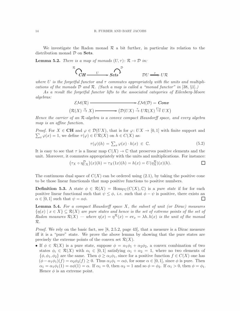
We investigate the Radon monad R a bit further, in particular its relation to thedistribution monad D on Sets.

Lemma 5.2. There is a map of monads (U, τ) : R → D in:

CH

R��

U // Sets

D

��DU

τ +3 UR

where U is the forgetful functor and τ commutes appropriately with the units and multipli-cations of the monads D and R. (Such a map is called a “monad functor” in [38, §1].)

As a result the forgetful functor lifts to the associated categories of Eilenberg-Moorealgebras:

EM(R) // EM(D) = Conv

(

R(X)α→ X

)

✤ //(

D(UX)τ→ UR(X)

Uα→ UX

)

Hence the carrier of an R-algebra is a convex compact Hausdorff space, and every algebramap is an affine function.

Proof. For X ∈ CH and ϕ ∈ D(UX), that is for ϕ : UX → [0, 1] with finite support and∑

x ϕ(x) = 1, we define τ(ϕ) ∈ UR(X) on h ∈ C(X) as:

τ(ϕ)(h) =∑

x ϕ(x) · h(x) ∈ C. (5.2)

It is easy to see that τ is a linear map C(X) → C that preserves positive elements and theunit. Moreover, it commutes appropriately with the units and multiplications. For instance:

(

τX ◦ ηDUX

)

(x)(h) = τX(1x)(h) = h(x) = U(ηRX)(x)(h).

The continuous dual space of C(X) can be ordered using (2.1), by taking the positive coneto be those linear functionals that map positive functions to positive numbers.

Definition 5.3. A state φ ∈ R(X) = HomPU(C(X),C) is a pure state if for for eachpositive linear functional such that ψ ≤ φ, i.e. such that φ− ψ is positive, there exists anα ∈ [0, 1] such that ψ = αφ.

Lemma 5.4. For a compact Hausdorff space X, the subset of unit (or Dirac) measures{η(x) | x ∈ X} ⊆ R(X) are pure states and hence is the set of extreme points of the set ofRadon measures R(X) — where η(x) = ηR(x) = evx = λh. h(x) is the unit of the monadR.

Proof. We rely on the basic fact, see [8, 2.5.2, page 43], that a measure is a Dirac measureiff it is a “pure” state. We prove the above lemma by showing that the pure states areprecisely the extreme points of the convex set R(X).

• If φ ∈ R(X) is a pure state, suppose φ = α1φ1 + α2φ2, a convex combination of twostates φi ∈ R(X) with αi ∈ [0, 1] satisfying α1 + α2 = 1, where no two elements of{φ, φ1, φ2} are the same. Then φ ≥ α1φ1, since for a positive function f ∈ C(X) one has(φ−α1φ1)(f) = α2φ2(f) ≥ 0. Thus α1φ1 = αφ, for some α ∈ [0, 1], since φ is pure. Thenα1 = α1φ1(1) = αφ(1) = α. If α1 = 0, then α2 = 1 and so φ = φ2. If α1 > 0, then φ = φ1.Hence φ is an extreme point.


• Suppose φ is an extreme point of R(X), i.e. that φ = α1φ1 + α2φ2 implies φ1 or φ2 = φ.Then if there is a positive linear functional ψ ≤ φ, we may take α1 = ψ(1) ≥ 0; sinceα1 = ψ(1) ≤ φ(1) = 1, we get α1 ∈ [0, 1]. If α1 = 0, then since ‖ψ‖ = ψ(1) = 0 we getψ = 0 and ψ = 0 ·φ. If α1 = 1, then (φ−ψ)(1) = 0, which since φ−ψ was assumed to bepositive implies φ − ψ = 0 and hence ψ = 1 · φ. Having dealt with those cases, we havethat α1 ∈ (0, 1), and so we have a state φ1 =

1α1ψ. We may take α2 = 1−α1 ∈ (0, 1) and

obtain a second state φ2 = 1α2(φ− ψ). By construction we have a convex decomposition

of φ = α1φ1 + α2φ2. Therefore either φ = φ1 = 1α1ψ or φ = φ2 = 1

α2(φ − ψ). In the

first case, ψ = α1φ, making φ pure. But also in the second case φ is pure, since we haveα2φ = φ− ψ and thus ψ = (1− α2)φ.

Lemma 5.5. Let X be a compact Hausdorff space.

(1) The maps τX : D(UX) → UR(X) from (5.2) are injective; as a result, the unit/Diracmaps η : X → R(X) are also injective.

(2) The maps τX : D(UX) UR(X) are dense.

Proof. For the first point, assume ϕ,ψ ∈ D(UX) satisfying τ(ϕ) = τ(ψ). We first show thatthe finite support sets are equal: supp(ϕ) = supp(ψ). Since X is Hausdorff, singletons areclosed, and hence finite subsets too. Suppose supp(ϕ) 6⊆ supp(ψ), so that S = supp(ϕ) −supp(ψ) is non-empty. Since S and supp(ψ) are disjoint closed subsets, there is by Urysohn’slemma a continuous function f : X → [0, 1] with f(x) = 1 for x ∈ S and f(x) = 0 forx ∈ supp(ψ). But then τ(ψ)(f) = 0, whereas τ(ϕ)(f) 6= 0.

Now that we know supp(ϕ) = supp(ψ), assume ϕ(x) 6= ψ(x), for some x ∈ supp(ϕ).The closed subsets {x} and supp(ϕ) − {x} are disjoint, so there is, again by Urysohn’slemma a continuous function f : X → [0, 1] with f(x) = 1 and f(y) = 0 for all y ∈ supp(ϕ).But then ϕ(x) = τ(ϕ)(f) = τ(ψ)(f) = ψ(x), contradicting the assumption.

We can conclude that the unit X → R(X) is also injective, since its underlying functioncan be written as the composite U(ηR) = τ ◦ ηD : UX D(UX) UR(X), because τ isa map of monads.

To show that the image of τX is dense, we proceed as follows. By Lemmas 5.4 and 5.2,the extreme points of R(X) are

{ηR(x) | x ∈ X} = {τ(

ηD(x)) | x ∈ X}

and are thus in the image of τ : D(UX) UR(X). Since every convex combination ofηR(x) comes from a formal convex sum ϕ ∈ D(UX), all convex combinations of extremepoints are in the image of τX . Using Proposition 2.5, R(X) can be considered an objectof CCLcvx, i.e. a compact convex subset of a locally convex space. Accordingly, we mayapply the Krein-Milman theorem [7, Proposition 7.4, page 142] to conclude the set of convexcombinations of extreme points is dense.

Lemma 5.6. Let X and Y be compact Hausdorff spaces. Each Eilenberg-Moore algebraα : R(X) → X is an affine function. For each continuous map f : X → Y , the functionR(f) : R(X) → R(Y ) is affine.

Proof. This follows from naturality of τ : DU ⇒ UR.

Proposition 5.7. Let α : R(X) → X and β : R(Y ) → Y be two Eilenberg-Moore algebrasof the Radon monad R. A function f : X → Y is an algebra homomorphism if and only iff is both continuous and affine.


As a result, the functor EM(R) → EM(D) = Conv from Lemma 5.2 is faithful, andan EM(D) map comes from an EM(R) map if and only if it is continuous.

We shall follow the convention of writing A(X,Y ) for the homset of continuous andaffine functions X → Y .

Proof. Clearly, each algebra map is both continuous and affine. For the converse, if f : X →Y is continuous, it is a map in the category CH of compact Hausdorff spaces. Since it isaffine, both triangles commute in:

D(UX) // τ

dense//

((◗◗◗◗

◗◗◗◗

◗◗◗◗

◗◗◗

R(X)

β◦R(f)��

f◦α��Y

Since Y is Hausdorff, there is at most one such map. Therefore f is an algebra map.

The category EM(R) of Eilenberg-Moore algebras of the Radon monad may thus beunderstood as a suitable category of convex compact Hausdorff spaces, with affine continu-ous maps between them. In the next section, we see how to use a result from [39] to relatethis to CCLcvx, which is a category of “concrete” convex sets. Using this theorem, it willbe shown that “observability” conditions like in [21, top of p. 169] always hold for algebrasof R.

5.1. Swirszcz’s Theorem and Noncommutative C∗-algebras. In this section we showthat the Radon monad arises from an adjunction in [39] enabling us to use Swirszcz’stheorem 3 from that paper to show that the categories CCLcvx and EM(R) are equivalent,which we can then apply to represent noncommutative C∗-algebras. The adjunction inquestion has U : CCLcvx → CH as the right adjoint, and the details of the constructionof the left adjoint are not given. In order to prove that R is the monad arising from thisadjunction, we need to know its unit and counit, so our next task is to define the left adjointexplicitly. Of course, any other left adjoint will be naturally isomorphic.

We begin as follows. We define S : CH → CCLcvx as S = Stat ◦ C. Hence R = U ◦ S.To show that S is the left adjoint to U , we use the unit and counit definition of an adjunction.We already know the unit, ηX : X → U(S(X)), as we gave it when defining the unit of R.To define the counit we use the notion of barycentre.

We can understand the intuitive notion of barycentre by thinking of a Radon probabilitymeasure µ on the unit square [0, 1]2. If we wanted to find the centre of mass of µ, which weshall call b ∈ [0, 1]2, we would take

bx =∫

[0,1]2xdµ and by =

∫

[0,1]2ydµ

for the x and y coordinates. We can see that x and y are continuous affine functions from[0, 1]2 → R, assigning each point to its x and y coordinate respectively. Therefore we canrewrite the above as

∫

[0,1]2xdµ = x(b) and

∫

[0,1]2ydµ = y(b).


In monadic terms, this means that both projections π1, π2 : [0, 1]2 → [0, 1] are maps of

Eilenberg-Moore algebras for the Radon monad, in the sense that the following diagramcommutes.

R([0, 1]2)

β��

R(πi) // R([0, 1])

α��

[0, 1]2πi

// [0, 1]

We write α for the algebra ν 7→∫

iddν, see also [20], and β for the product algebra structure,given by µ 7→ 〈

∫

π1dµ,∫

π2dµ〉 = 〈∫

xdµ,∫

ydµ〉.If we generalize π1 and π2 to arbitary real-valued continuous affine functions on X, and

reinterpret Radon measures as functionals (as in the start of §5), we get the idea behindthe following standard definition.

Definition 5.8. If X ∈ CCLcvx and φ ∈ S(U(X)), then a point x ∈ X is a barycentre forφ if for all continuous affine functions f from X → R we have that φ(f) = f(x).

The theorem that every φ has a barycentre when X is a compact subset of a locallyconvex space is standard and is proven in [3, proposition I.2.1 and I.2.2].

We will require the following important lemma, one of sevaral variants of the Hahn-Banach separation lemma, and some of its corollaries, which give an affine analogue ofUrysohn’s lemma for objects in CCLcvx.

Lemma 5.9. If V is a locally convex topological vector space, X a closed convex subset andY a compact convex subset that is disjoint from X, then there exists a continuous linearfunctional φ : V → R and α ∈ R such that φ(X) ⊆ (α,∞) and φ(Y ) ⊆ (−∞, α).

For proof, see either [7, theorem IV.3.9] or [36, II.4.2 corollary 1].

Corollary 5.10. Let (K,V ) ∈ Obj(CCLcvx). In the following X,Y will be arbitrary closeddisjoint convex subsets of K, x, y arbitrary distinct points of K.

(i) There is a φ ∈ A(K,R) and an α ∈ R such that φ(X) ⊆ (α,∞) and φ(Y ) ⊆ (−∞, α).(ii) There is a φ ∈ A(K,R) such that φ(x) 6= φ(y).(iii) There is a φ ∈ CCLcvx(K, [0, 1]) and an α ∈ R such that φ(X) ⊆ (α, 1] and φ(Y ) ⊆

[0, α).(iv) There is a φ ∈ CCLcvx(K, [0, 1]) such that φ(x) 6= φ(y).

Proof.

(i) Apply Lemma 5.9 to obtain φ′ : V → R separating X from Y . Since K has thesubspace topology, φ = φ′|K is continuous, and since φ′ is linear, φ is affine, henceφ ∈ A(K,R). We also keep the properties that φ(X) ⊆ (α,∞) and φ(Y ) ⊆ (−∞, α).

(ii) This follows directly from (i), using the fact that points are compact and convex.(iii) We use (i) and obtain φ′ ∈ A(K,R) and α′ ∈ R. Since the image of a compact space

is compact, and a compact subset of R is closed and bounded, the numbers

β↑ = supφ′(K) β↓ = inf φ′(K)

exist, and φ′ can be considered as an affine continuous map K → [β↓, β↑]. We define

φ(k) =φ(k)− β↓

β↑ − β↓


if β↑ 6= β↓, otherwise we define it without dividing by anything, though this can onlyhappen if one of X or Y is empty. The image of φ is contained in [0, 1], and φ is affineand continuous, being the composition of affine and continuous maps. We define

α =α′ − β↓

β↑ − β↓

again not doing the division if it is zero. We have that φ(X) ⊆ (α,∞), and sincethe image of φ is contained in [0, 1], this implies φ(X) ⊆ (α, 1]. The proof thatφ(Y ) ⊆ [0, α) is similar.

(iv) This is proven using (iii), again using the fact that points are closed, convex sets.

Using the properties proven above, we can start to define the counit of the adjunction.

Lemma 5.11.

(i) For every φ ∈ S(U(X)) the barycentre is unique. The function εX : S(U(X)) → X

mapping φ to its barycentre is well defined.(ii) This εX is an affine map.

Proof.

(i) We show the barycentre is unique as follows. Let (V,X) be an object of CCLcvx,V being the locally convex space and X the compact convex subset. Let x, x′ ∈ X

be barycentres of φ ∈ S(U). Suppose for a contradiction that x 6= x′. By corollary5.10 (ii), there is an f ∈ A(X,R) such that f(x) 6= f(x′). Since x and x′ are bothbarycentres of φ,

f(x) = φ(f) = f(x′)

a contradiction. So we have x = x′. Therefore εX is well-defined, at least as a functionbetween sets.

(ii) To show that εX is affine, consider two Radon measures φ,ψ ∈ S(U(X)), such thatεX(φ) = x and εX(ψ) = y, i.e. these are the barycentres. To show that εX(αφ+ (1−α)ψ) = αεX(φ) + (1− α)εX (ψ), we will show that αx+ (1− α)y is the barycentre ofαφ+ (1− α)ψ. Given an continuous affine function f : X → R, we have

(αφ + (1− α)ψ)(f) = αφ(f) + (1− α)ψ(f) = αx+ (1− α)y

so εX is affine.

Lemma 5.12. The barycentre map εX is continuous, hence a map in CCLcvx.

Proof. We now show that εX is continuous. We use the filter-theoretic definition of continu-ity. Given φ ∈ S(U(X)), with barycentre x, we want to show that for every neighbourhoodV of x, there is a neighbourhood U of φ such that εX(U) ⊆ V . It suffices to prove thisfor a chosen set of basic neighbourhoods, so we choose open neighbourhoods for X andfor S(U(X)) we choose finite intersections of elements of the following subbasis of closedneighbourhoods:

Uf,α,ǫ = {ψ ∈ S(U(X)) | |ψ(f)− α| ≤ ǫ}

where f ∈ C(U(X)), α ∈ R and ǫ ∈ (0,∞).We find the neighbourhood of φ using a compactness argument.Consider the following subset of X.

⋂

f∈A(X,R)ǫ>0

εX(Uf,f(x),ǫ)


Since φ ∈ Uf,f(x),ǫ for all values of f and ǫ, we have that x is in this intersection. We willshow that

⋂

f∈A(X,R)ǫ>0

εX(Uf,f(x),ǫ) = {x} (5.3)

As we already know x is an element of the left hand side, we will show that if x′ ∈ X andx′ 6= x, then x′ is not an element of the left hand side. So since x 6= x′, by Corollary 5.10(ii)there is an f ∈ A(X,R) such that f(x) 6= f(x′). We let

ǫ =|f(x)− f(x′)|

3> 0 (5.4)

We show that x′ 6∈ εX(Uf,f(x),ǫ) and therefore is not in (5.3) by showing there is an openset containing x′ that is disjoint from εX(Uf,f(x),ǫ). The open set we choose is

f−1((f(x′)− ǫ, f(x′) + ǫ))

which is open because f is continuous. Assume for a contradiction that there is somex′′ ∈ f−1((f(x′)− ǫ, f(x′) + ǫ)) ∩ εX(Uf,f(x),ǫ). This means that

|f(x′)− f(x′′)| < ǫ (5.5)

and there is some ψ ∈ Uf,f(x),ǫ of which x′′ is the barycentre, i.e. for all g ∈ A(X,R)ψ(g) = g(x′′). Therefore it must be the case that ψ(f) = f(x′′), and so the inequalityderiving from ψ ∈ Uf,f(x),ǫ, which is |ψ(f) − f(x)| ≤ ǫ becomes |f(x′′) − f(x)| ≤ ǫ. If wecombine this with (5.5) and use the triangle inequality, we get |f(x′) − f(x)| ≤ 2ǫ, whichcontradicts |f(x) − f(x′)| ≥ 3ǫ from (5.4). Therefore the assumption that x′′ could exist

is wrong, so x′ is in an open set outside εX(Uf,f(x),ǫ), and hence x′ 6∈ εX(Uf,f(x),ǫ). Thisestablishes that (5.3) is the case.

Now consider X \ V , which is a closed set that does not contain x, since V is an openneighbourhood of x. We therefore have

∅ = (X \ V ) ∩⋂

f∈A(X,R)ǫ>0

εX(Uf,f(x),ǫ) =⋂

f∈A(X,R)ǫ>0

(X \ V ) ∩ εX(Uf,f(x),ǫ)

The right hand side is a family of closed subsets of a compact space with empty inter-section. Therefore there is a finite subfamily also having empty intersection. We use thenumbers i ∈ {1, . . . , n} as an index set, and take {ǫi}, {fi} such that we have

∅ =

n⋂

i=1

(X \ V ) ∩ εX(Ufi,fi(x),ǫi) = (X \ V ) ∩n⋂

i=1

εX(Ufi,fi(x),ǫi)

Therefore we have

εX

(

n⋂

i=1

Ufi,fi(x),ǫi

)

⊆n⋂

i=1

εX(Ufi,fi(x),ǫi) ⊆n⋂

i=1

εX(Ufi,fi(x),ǫi) ⊆ V

Since V was an arbitrary open neighbourhood of εX(φ), we have that εX is continuous atφ. Since the choice of φ was arbitrary, εX is continuous.


Lemma 5.13. The family {εX} defines a natural transformation ε : S ◦ U ⇒ Id.

Proof. We must show that

S(U(X))ǫX //

S(U(f))��

X

f

��S(U(Y ))

ǫY// Y

Suppose that φ ∈ S(U(X)) and εX(φ) = x, i.e. x is the barycentre of φ. It suffices to show

that f(x) is the barycentre of S(U(f)(φ). Let h ∈ C(Y ), and we have by definition that

S(U(f))(φ)(h) = φ(h ◦ f)

We want to show that if h is affine, then S(U(f))(φ)(h) = h(f(x)), as this would showf(x) is the barycentre. Since h ◦ f is the composite of continuous, affine functions, itis also continuous and affine, and so, using that x is the barycentre of φ, we have thatφ(h ◦ f) = (h ◦ f)(x) = h(f(x)), which is what we were required to prove.

Taken together, the preceding three lemmas define the counit. We can now move on toshowing that this is actually an adjunction.

Theorem 5.14. The functor S : CH → CCLcvx is the left adjoint to U : CCLcvx → CH

Proof. We show that the unit-counit diagrams commute.First we must show that the following commutes:

UYηUY //

idUY &&▲▲▲▲

▲▲▲▲

▲▲▲

U(S(U(Y )))

UεY��

UY

In other words, we must show that for all y ∈ UY , y is the barycentre of ηUY (y). Using thedefinition of η, we have that for any affine continuous function f : X → R that

ηUY (x)(f) = f(x)

because that is already true for all continuous functions f ∈ C(X). Therefore x is thebarycentre of ηUY (x), and so the diagram commutes.

The second diagram we must consider is the following:

S(X)S(ηX ) //

idS(X) %%▲▲

▲▲▲▲

▲▲▲▲

S(U(S(X)))

ǫS(X)

��

S(X)

This time, we need to show that φ ∈ S(X) is the barycentre of the measure S(ηX)(φ). So

consider an affine continuous function k : S(X) → R. We want to show that S(ηX)(φ)(k) =

k(φ) for all φ ∈ S(X). To do this, we use Lemma 5.5. We show the diagram commutes on


the convex combinations of extreme points, and since this is a dense subset, the diagramcommutes by continuity. So let {x1, . . . xn} be a finite subset of X, and

n∑

i=1

αiηX(xi)

a finite convex combination of extreme points of S(X). Now

S(ηX)

(

n∑

i=1

αiηX(xi)

)

(k) =

(

n∑

i=1

αiηX(xi)

)

(k ◦ ηX)

=

n∑

i=1

αiηX(xi)(k ◦ ηX)

=n∑

i=1

αik(ηX(xi))

= k

(

n∑

i=1

(ηX(xi))

)

with the last step holding because k is an affine function.As explained before, this shows S(ηX)(φ)(k) = k(φ) for all φ ∈ S(X), and hence the

diagram commutes. Thus we have that S is the left adjoint to U .

Now that we have defined the adjunction S ⊣ U , we can move on to proving that R isnot only the same functor as the monad derived from S ⊣ U but also the same as a monad.In order to do this, we require a few lemmas concerning the definition of µ we gave at thestart of Section 5. The map µ was defined using λh. h(v). Since we need to prove certainproperties about it, we give this map a name, and generalize it somewhat for later use. IfA is a (possibly noncommutative) C∗-algebra, we define

Asa ζA // A(Stat(A),R) as ζA(a)(φ) = φ(a).

In the special case we had earlier, we were using ζC(X) for a compact Hausdorff space X,since C(X)sa = CR(X), the real-valued functions. We can see that

µX(g)(v) = g(ζC(X)(v)). (5.6)

Lemma 5.15. The map ζA is a bijection between Asa and A(Stat(A),R). ζC(X) is a bijec-

tion between CR(X) and A(S(X),R). In fact, the bijection is an isomorphism of orderedR-vector spaces with unit, taking these to be defined pointwise on A(Stat(A),R).

The proof can be found in [2, Proposition 2.3]. It was originally proved by Kadison [25,Lemma 4.3, Remark 4.4] and is often stated for complete order-unit spaces (such as in [3,Theorem II.1.8]), though it was originally intended for use with C∗-algebras, as here.

Theorem 5.16. The monad : CH → CH given by S ⊣ U is the Radon monad R.

Proof. We have by definition that R = U S and η = η. Therefore we only need to showthat µ = UεS. What we need to show then, is that if X is a compact Hausdorff space andφ ∈ S(U(S(X))), then µ(φ) is the barycentre of φ. That is to say, for all f ∈ A(S(X),R),


φ(f) = f(µX(φ)). Using Lemma 5.15, we reduce to showing that for all f ∈ CR(X), wehave φ(ζX(f)) = ζX(f)(µX(φ)). Using (5.6), we have

ζX(f)(µX(φ)) = µX(φ)(f) = φ(ζX(f))

as required.

Theorem 5.17 (Swirszcz’s theorem). The forgetful functor U : CCLcvx → CH is monadic,

i.e. CCLcvx ≃ EM(U ◦ S). By Theorem 5.16, CCLcvx ≃ EM(R).

This comes from [39, Theorem 3]. A proof not using any monadicity theorems can befound in [37, Proposition 7.3].

5.1.1. Non-commutative C∗-algebras and EM(R). In the following section we shall showthat the category CstarPU embeds fully and faithfully in EM(R). To do this, we use thefact that EM(R) ≃ CCLcvx, and also the functor Stat : CstarPU → CCLcvx.

We begin with a standard separation result from the theory of C∗-algebras.

Lemma 5.18. If A is a C∗-algebra, and a, b ∈ A, then

φ(a) = φ(b)

for all φ ∈ Stat(A) implies a = b. In other words, A is separated by its states, or A has“sufficiently many states”.

Proof. In [24, theorem 4.3.4 (i)] we have that if φ(a) = 0 for all φ ∈ Stat(A), then a = 0.We simply apply this to a− b.

On the set A(X,C), for X ∈ Obj(CCLcvx), we can define a C-vector space structure,a positive cone, and a distinguished unit, simply by using the fact that C has these thingsand defining them pointwise. The positive cone is [0,∞) ⊆ C and the unit is 1. Given thesedefinitions, we can prove the complexification of Lemma 5.15.

Lemma 5.19. For each C∗-algebra A, the map ξA : A→ A(Stat(A),C), defined as

ξA(a)(φ) = φ(a)

is an isomorphism of complex vector spaces preserving the positive cone and unit in bothdirections.

Proof. First we show that the map ξA is C-linear and preserves ∗. For C-linearity, let z ∈ C,φ ∈ Stat(A) and a ∈ A. Then

ξA(za)(φ) = φ(za) = zφ(a) = zξA(a)(φ),

so ξA(za) = zξA(a).To show that it preserves ∗, where for f ∈ A(Stat(A),C), f∗ is calculated pointwise, we

use the fact that every positive linear functional on A, and hence every state, is self-adjoint,as described in Lemma 2.2, i.e. φ(a∗) = φ(a).

Thus we have

ξA(a∗)(φ) = φ(a∗) = φ(a) = ξA(a)(φ) = ξA(a)

∗(φ).

and so ξA(a∗) = ξA(a)

∗.


From Lemma 5.15 we have that ξ restricts to an isomorphism ζ : Asa ∼= A(Stat(A),R)as an ordered vector space with unit. We extend this to complex numbers as follows. Givena ∈ A, we can define its real and imaginary parts as

ℜ(a) =a+ a∗

2ℑ(a) =

a− a∗

2i

and we see that ℜ(a) + iℑ(a) = a. Similarly, using pointwise complex conjugation as ∗, wecan define real and imaginary parts of an affine continuous map from Stat(A) → C, andthe self-adjoint elements are maps Stat(A) → C. Since we know that ηX has an inverse forself-adjoint elements, we can define the inverse as

ξ−1A (f + ig) = ξ−1

A (f) + iξ−1A (g)

where f, g are self-adjoint.We show this is the inverse of ξA. For one way

ξA(ξ−1A (f + ig)) = ξA(ξ

−1A (f) + iξ−1

A (g))

= ξA(ξ−1A (f)) + iξA(ξ

−1A (g))

= f + ig.

For the other way, with a, b ∈ Asa,

ξ−1A (ξA(a+ ib)) = ξ−1

A (ξA(a) + iξA(b))

= ξ−1A (ξA(a)) + iξ−1

A (ξA(b))

= a+ ib,

where the definition of ξ−1A can be applied since ξA preserves ∗ and hence preserves self-

adjointness, so ξA(a) and ξA(b) are both self-adjoint.

We will require the following fact in a moment.

Lemma 5.20. If B is a C∗-algebra, b′ ∈ A(Stat(B),C), then for all φ ∈ Stat(B)

φ(ξ−1B (b′)) = b′(φ).

Proof. By Lemma 5.19, we have that there is some b ∈ B such that b′ = ξB(b). Then wehave

φ(ξ−1B (b′)) = φ(ξ−1

B (ξB(b))) = φ(b) = ξB(b)(φ) = b′(φ).

We can now prove that Stat is full and faithful, and hence (CstarPU)op embeds fully in

EM(R).

Theorem 5.21. The state space functor Stat : (CstarPU)op → CCLcvx is full and faithful.

Proof.

• For faithfulness, suppose we have f, g : A → B in CstarPU, such that Stat(f) = Stat(g).We have that Stat(f)(φ) = Stat(g)(φ) for all φ ∈ Stat(B), which, expanding the defini-tions, gives that φ ◦ f = φ ◦ g for all φ ∈ Stat(B). Now, we have that for all a ∈ A

and φ ∈ Stat(B), that φ(f(a)) = φ(g(a)). By Lemma 5.18, we have that for all a ∈ A,f(a) = g(a), and therefore f = g.


• For fullness, let g : Stat(B) → Stat(A) be an affine, continuous map. We must find a mapf : A → B such that Stat(f) = g. We take the map f = ξ−1

B ◦ A(g,C) ◦ ξA : A → B.First we must prove this map is positive, C-linear, and unital. We know from Lemma5.19 that, being isomorphisms, ξA and ξ−1

B are C-linear (with the pointwise structureon A(Stat(A),C)) and preserve the positive cone and unit. Therefore we only needto show that A(g,C) has these properties to verify them for f . For C-linearity, leta1, a2 ∈ A(Stat(A),C), and z1, z2 ∈ C. Then for each φ ∈ Stat(B)

A(g,C)(z1a1 + z2a2)(φ) = ((z1a1 + z2a2) ◦ g)(φ)

= (z1a1 + z2a2)(g(φ))

= z1a1(g(φ)) + z2a2(g(φ))

= z1A(g,C)(a1)(φ) + z2A(g,C)(a2)(φ)

= (z1A(g,C)(a1) + z2A(g,C)(a2))(φ),

and soA(g,C)(z1a1 + z2a2) = z1A(g,C)(a1) + z2A(g,C)(a2),

which is to say, A(g,C) is C-linear.The unit of A(Stat(A),C) is given by the function 1: Stat(A) → C that maps every

element of Stat(A) to 1 ∈ C. We must show that A(g,C) preserves this unit. Givenφ ∈ Stat(B), we have

A(g,C)(1)(φ) = 1(g(φ)) = 1,

so A(g,C)(1) takes the value 1 ∈ C for all φ ∈ Stat(B), and hence it is the unit inA(Stat(B),C).

The positive elements of A(Stat(A),C) are given by functions whose image is containedin the positive reals, [0,∞) ⊆ C. We need to show that if a ∈ A(Stat(A), [0,∞)), then sois A(g,C)(a). This is easily accomplished as before. If φ ∈ Stat(B), then

A(g,C)(a)(φ) = (a ◦ g)(φ) = a(g(φ)).

Since g(φ) ∈ Stat(A), we have that a(g(φ)) ∈ [0,∞) by the assumption on a, and soA(g,C)(a) is a positive element of A(Stat(B),C). All these conditions, taken together,show that f is a CstarPU map from A to B.

Now we show that Stat(f) = g. Let φ ∈ Stat(B) and a ∈ A. Then

Stat(f)(φ)(a) = Stat(ξ−1B ◦ A(g,C) ◦ ξA)(φ)(a)

= (φ ◦ ξ−1B ◦ A(g,C) ◦ ξA)(a)

= φ(ξ−1B (A(g,C)(ξA(a))))

= φ(ξ−1B (ξA(a) ◦ g)),

applying Lemma 5.20, we continue

Stat(f)(φ)(a) = (ξA(a) ◦ g)(φ)

= ξA(a)(g(φ))

= g(φ)(a).

Since this holds for all φ and a, we have the required equality Stat(f) = g, proving Statis full.


Alfsen, Hanche-Olsen and Shultz have characterized the essential image of Stat [4, Corollary8.6]. We do not give the characterization here as it involves many further definitions. Sincethere are PU-maps that are not completely positive, Stat is not a full functor when restrictedtoCstarcPU. In fact, whether a map is completely positive or not depends on the orientation(in the sense of [4]) and cannot be defined purely from the EM(R) structure of the statespace. This can be seen by the fact that the transpose map, the archetypal positive but notcompletely positive map, is self-inverse, and hence an isomorphism as a PU map, and so bythe above result defines an isomorphism in EM(R) on the state space.

6. States and effects

We start with a simple observation.

Lemma 6.1. The unit interval [0, 1] is a compact convex subset of the locally convex space R,and therefore carries a R-algebra structure by Theorem 5.17. The algebra map R([0, 1]) →[0, 1] maps each measure to its mean value.

For an arbitrary R-algebra X, the homset of algebra maps:

EM(R)(

X, [0, 1])

= A(X, [0, 1])

is an effect module, with pointwise operations. Recall from Proposition 5.7 that this homsetis the affine and continuous functions X → [0, 1]. Taken all together, we have defined afunctor A(−, [0, 1]) : EM(R) → EMod

op.

In [21] it is shown that for an effect moduleM , the homset EMod(M, [0, 1]) is a convexcompact Hausdorff space. In fact, it carries an R-algebra structure:

R(

EMod(M, [0, 1])) αM // EMod(M, [0, 1])

h✤ // λx ∈M.h(evx)

where evx = λv. v(x) : C(

EMod(M, [0, 1]))

→ C. For each map of effect modules f : M →M ′ one obtains a map of R-algebras (−) ◦ f : EMod(M ′, [0, 1]) → EMod(M, [0, 1]). Wethus obtain the following situation:

EModop

EMod(−,[0,1])--

⊤ EM(R)A(−,[0,1])

mm EModop

EMod(−,[0,1])--

⊤ EM(R)A(−,[0,1])

mm

Kℓ(R)

Cont(−,[0,1])

ee❑❑❑❑❑❑❑❑❑❑❑

99ttttttttt(CstarPU)

op

[0,1](−)

gg❖❖❖❖❖❖❖❖❖❖❖❖ Stat

77♣♣♣♣♣♣♣♣♣♣♣

(6.1)Such diagrams appear in [18] as a categorical representation of the duality between statesand effects, with the Schrodinger picture on the right vertex of the triangle, and the Heisen-berg picture on the left vertex of the triangle (see also [20]). In these diagrams:

• The map Kℓ(R) → EModop on the left is the “predicate” functor, sending a space X tothe predicates on X, given by the effect module Cont(X, [0, 1]) of continuous functionsX → [0, 1], or for C∗-algebras mapping A to the effects [0, 1]A. For C

∗-algebras this wasshown to be full and faithful in Lemma 2.6, and for Kℓ(R) we combine Lemma 2.6 and


Theorem 5.1:

EMod(

Cont(Y, [0, 1]),Cont(X, [0, 1]))

= EMod(

[0, 1]C(Y ), [0, 1]C(X)

)

∼= HomPU

(

C(Y ), C(X))

∼= Kℓ(R)(

X,Y)

.

• The “state” functor Kℓ(R) → EM(R) is the standard full and faithful “comparison”functor from a Kleisli category to a category of Eilenberg-Moore algebras. In the C∗-algebra case it is the functor Stat, combined with the equivalence from Theorem 5.17. Itis full and faithful by Theorem 5.21.

• The diagrams in (6.1) commute (up-to-isomorphism) in one direction. For Kℓ(R) wehave:

EMod(

Cont(X, [0, 1]), [0, 1])

= EMod(

[0, 1]C(X), [0, 1]C)

∼= HomPU

(

C(X),C) = R(X),

and similarly for CstarPU we have

EMod([0, 1]A, [0, 1]) ∼= CstarPU(A,C) by Lemma 2.6

= Stat(A)

• The diagrams in (6.1) also commute (again, up-to-isomorphism) in the other direction,i.e. A(R(X), [0, 1]) ∼= Cont(X, [0, 1]) and A(Stat(A), [0, 1]) ∼= [0, 1]A. The former followsfrom the latter by taking A = C(X), so we reduce to the latter. By Lemma 5.19 we havethat A ∼= A(Stat(A),C) as unital ordered vector spaces. We can then restrict both sidesto their unit intervals and obtain an isomorphism [0, 1]A ∼= A(Stat(A), [0, 1]).

We summarise what we have just shown.

Theorem 6.2. The diagrams (6.1) are commuting “state-and-effect” triangles.

Final remarks

The main contribution of this article lies in establishing a connection between two differ-ent worlds, namely the world of theoretical computer scientists using program languagesemantics (and logic) via monads, and the world of mathematicians and theoretical physi-cists using C∗-algebras. This connection involves the distribution monad D on Sets, whichis heavily used for modeling discrete probabilistic systems (Markov chains), in the finite-dimensional case (see Proposition 4.3) and the less familiar Radon monad R on compactHausdorff spaces (see Theorem 5.1). These results apply to both commutative and noncom-mutative C∗-algebras, but only to positive unital maps. Follow-up research will concentrateon characterizing completely positive maps in the noncommutative case.

Acknowledgements. The authors wish to thank Hans Maassen, Jorik Mandemaker andKlaas Landsman for helpful discussions.

This research has been financially supported by the Netherlands Organisation for Sci-entific Research (NWO) under TOP-GO grant no. 613.001.013 (The logic of compositequantum systems).


References

[1] S. Abramsky and B. Coecke. A categorical semantics of quantum protocols. In K. Engesser, Dov M.Gabbai, and D. Lehmann, editors, Handbook of Quantum Logic and Quantum Structures, pages 261–323.North Holland, Elsevier, Computer Science Press, 2009.

[2] E.M. Alfsen and F.W. Shultz. State Spaces of Operator Algebras. Birkhauser, 2001.[3] Erik M. Alfsen. Compact Convex Sets and Boundary Integrals. Ergebnisse der Mathematik und ihrer

Grenzgebiete. Springer, 1971.[4] Erik M. Alfsen, Harald Hanche-Olsen, and Frederic W. Shultz. State Spaces of C∗-algebras. Acta Math-

ematica, 144(1):267–305, 1980.[5] W. Arveson. An Invitation to C

∗-Algebra. Springer-Verlag, 1981.[6] Patrick Billingsley. Convergence of Probability Measures. John Wiley and Sons, 1968.[7] J.B. Conway. A Course In Functional Analysis, Second Edition, volume 96 of Graduate Texts in Math-

ematics. Springer Verlag, 1990.[8] J. Dixmier. C∗-Algebras, volume 15 of North-Holland Mathematical Library. North-Holland Publishing

Company, 1977.[9] A. Dvurecenskij and S. Pulmannova. New Trends in Quantum Structures. Kluwer Acad. Publ., Dor-

drecht, 2000.[10] D. J. Foulis and M.K. Bennett. Effect algebras and unsharp quantum logics. Found. Physics,

24(10):1331–1352, 1994.[11] D. H. Fremlin. Measure Theory, Volume 4. http://www.essex.ac.uk/maths/people/fremlin/mt.htm,

2003.[12] Tobias Fritz. A Presentation of the Category of Stochastic Matrices. http://arxiv.org/abs/0902.2554,

2009.[13] J-Y. Girard. Geometry of Interaction V: Logic in the hyperfinite factor. Theor. Comput. Sci.,

412(20):1860–1883, April 2011.[14] M. Giry. A categorical approach to probability theory. In B. Banaschewski, editor, Categorical Aspects

of Topology and Analysis, volume 915 of Lecture Notes in Mathematics, pages 68–85. Springer BerlinHeidelberg, 1982.

[15] Paul R. Halmos. Measure Theory. Number 18 in Graduate Texts in Mathematics. Springer, 1950.[16] T. Heinosaari and M. Ziman. The Mathematical Language of Quantum Theory. From Uncertainty to

Entanglement. Cambridge Univ. Press, 2012.[17] M. Horodecki, P. Horodecki, and R. Horodecki. Separability of Mixed States: Necessary and Sufficient

Conditions. Physics Letters A, 223(12):1 – 8, 1996.[18] B. Jacobs. Introduction to Coalgebra. Towards Mathematics of States and Observations. 2012. Book, in

preparation; version 2.0 available from www.cs.ru.nl/B.Jacobs/CLG/JacobsCoalgebraIntro.pdf .[19] B. Jacobs. Involutive categories and monoids, with a GNS-correspondence. Found. of Physics, 42(7):874–

895, 2012.[20] B. Jacobs. Measurable spaces and their effect logic. In Logic in Computer Science. IEEE, Computer

Science Press, 2013.[21] B. Jacobs and J. Mandemaker. The expectation monad in quantum foundations. In B. Jacobs,

P. Selinger, and B. Spitters, editors, Quantum Physics and Logic (QPL) 2011, volume 95 of Elect.Proc. in Theor. Comp. Sci., pages 143–182, 2012.

[22] B. Jacobs and J. Mandemaker. Relating operator spaces via adjunctions. In J. Chubb Reimann,V. Harizanov, and A. Eskandarian, editors, Logic and Algebraic Structures in Quantum Computingand Information, Lect. Notes in Logic. Cambridge Univ. Press, 2013. See arxiv.org/abs/1201.1272.

[23] P. Johnstone. Stone Spaces. Number 3 in Cambridge Studies in Advanced Mathematics. CambridgeUniv. Press, 1982.

[24] R. Kadison and J. Ringrose. Fundamentals of the Theory of Operator Algebras. Academic Press, 1983.[25] Richard V. Kadison. Transformations of States in Operator Theory and Dynamics. Topology, 3, Supple-

ment 2(0):177 – 198, 1965.[26] A. Kock. On double dualization monads. Math. Scand., 27:151–165, 1970.[27] H. Maassen. Quantum probability and quantum information theory. In F. Benatti, M. Fannes, R. Flo-

reanini, and D. Petritis, editors, Quantum Information, Computation and Cryptography, number 808 inLect. Notes Physics, pages 65–108. Springer, Berlin, 2010.

http://www.essex.ac.uk/maths/people/fremlin/mt.htm

http://arxiv.org/abs/0902.2554

www.cs.ru.nl/B.Jacobs/CLG/JacobsCoalgebraIntro.pdf


[28] E. Manes. A triple-theoretic construction of compact algebras. In B. Eckman, editor, Seminar on Triplesand Categorical Homolgy Theory, number 80 in Lect. Notes Math., pages 91–118. Springer, Berlin, 1969.

[29] M. Mislove, J. Ouaknine, D. Pavlovic, and J. Worrell. Duality for Labelled Markov Processes. In IgorWalukiewicz, editor, Foundations of Software Science and Computation Structures, volume 2987 ofLecture Notes in Computer Science, pages 393–407. Springer Berlin Heidelberg, 2004.

[30] Michael Mislove. Probabilistic Monads, Domains and Classical Information. In Elham Kashefi, JeanKrivine, and Femke van Raamsdonk, editors, Proceedings 7th International Workshop on Developmentsof Computational Methods, Zurich, Switzerland, 3rd July 2011, volume 88 of Electronic Proceedings inTheoretical Computer Science, pages 87–100. Open Publishing Association, 2012.

[31] E. Moggi. Notions of computation and monads. Inf. & Comp., 93(1):55–92, 1991.[32] J. Wick Pelletier and J. Rosicky. On the Equational Theory of C∗-algebras. Algebra Universalis, 30:275–

284, 1993.[33] W. Rudin. Real and Complex Analysis. McGraw-Hill Book Company, 1987. Third, International edition.[34] B. Russo and H.A. Dye. A Note on Unitary Operators in C

∗-algebras. Duke Math. J., 33:413–416, 1966.[35] S. Sakai. C∗-algebras and W

∗-algebras, volume 60 of Ergebnisse der Mathematik und ihrer Grenzgebiete.Springer, 1971.

[36] Helmut H. Schaefer. Topological Vector Spaces, volume 3 of Graduate Texts in Mathematics. SpringerVerlag, 1966.

[37] Z. Semadeni. Monads and their Eilenberg-Moore Algebras in Functional Analysis, volume 33 of Queen’sPapers in Pure and Applied Mathematics. Queen’s University at Kingston, Ontario, Canada, 1973.

[38] R. Street. The formal theory of monads. Journ. of Pure & Appl. Algebra, 2:149–169, 1972.

[39] T. Swirszcz. Monadic Functors and Convexity. Bulletin de l’Academie Polonaise des Sciences, Serie desSciences Math. Astr. et Phys., 22(1):39–42, 1974.

[40] A. Westerbaan. Quantum Programs as Kleisli Maps. http://arxiv.org/abs/1501.01020.

This work is licensed under the Creative Commons Attribution-NoDerivs License. To viewa copy of this license, visit http://creativecommons.org/licenses/by-nd/2.0/ or send aletter to Creative Commons, 171 Second St, Suite 300, San Francisco, CA 94105, USA, orEisenacher Strasse 2, 10777 Berlin, Germany

FROM KLEISLI CATEGORIES TO COMMUTATIVE … · c R. Furber and Bart Jacobs CC Creative Commons. 2 R....

Documents

Transcript of FROM KLEISLI CATEGORIES TO COMMUTATIVE … · c R. Furber and Bart Jacobs CC Creative Commons. 2 R....