From Euler, Ritz, and Galerkin to Modern Computingzxu2/acms60790S13/Euler-Ritz-Galerkin.pdf · FROM...
40
SIAM REVIEW c 2012 Society for Industrial and Applied Mathematics Vol. 54, No. 4, pp. 000–000 From Euler, Ritz, and Galerkin to Modern Computing ∗ Martin J. Gander † Gerhard Wanner † Abstract. The so-called Ritz–Galerkin method is one of the most fundamental tools of modern com- puting. Its origins lie in Hilbert’s “direct” approach to the variational calculus of Euler– Lagrange and in the thesis of Walther Ritz, who died 100 years ago at the age of 31 after a long battle with tuberculosis. The thesis was submitted in 1902 in G¨ottingen, during a period of dramatic developments in physics. Ritz tried to explain the phenomenon of Balmer series in spectroscopy using eigenvalue problems of partial differential equations on rectangular domains. While this physical model quickly turned out to be completely obsolete, his mathematics later enabled him to solve difficult problems in applied sciences. He thereby revolutionized the variational calculus and became one of the fathers of modern computational mathematics. We will see in this article that the path leading to modern computational methods and theory involved a long struggle over three centuries requiring the efforts of many great mathematicians. Key words. Walther Ritz, variational calculus, finite element method AMS subject classifications. AUTHOR: PLEASE PROVIDE DOI. 10.1137/100804036 1. The Variational Calculus of Euler and Lagrange. The most well-known con- tribution of Walther Ritz is the development of a systematic approach for solving variational problems. His methods transformed variational calculus from a theoreti- cal tool to one of practical importance, and they are the precursor to many algorithms in modern scientific computing. Going back in history, we will see how variational calculus started in 1696 with the famous challenge concerning the brachystochrone problem, which led to endless disputes between the Bernoulli brothers. Euler [12] gave in 1744 a general solution to variational problems in the form of a differential equation. Eleven years later, the nineteen-year-old Lagrange then communicated, in a famous letter to Euler, an elegant justification for this equation. The prodigious contributions of Euler concerning the analytic and numerical solutions of differential equations, in particular, his Institutiones Calculi Integralis [13] from 1768–1770, then added the finishing touch to the theory. 1.1. The Brachystochrone Problem. In 1696, Johann Bernoulli challenged the mathematical world (which included his brother Jacob) with the following problem (see Figure 1.1): Given two fixed points A and B in a vertical plane, find a curve AMB such that a body gliding on it under gravity, starting from A, arrives after the ∗ Received by the editors July 30, 2010; accepted for publication (in revised form) September 29, 2011; published electronically November 8, 2012. http://www.siam.org/journals/sirev/54-4/80403.html † Section de Math´ ematiques, Universit´ e de Gen` eve, CP 64, 1211 Gen` eve (Martin.Gander@ unige.ch, [email protected]). 1
-
Upload
hoangnguyet -
Category
Documents
-
view
250 -
download
1
Transcript of From Euler, Ritz, and Galerkin to Modern Computingzxu2/acms60790S13/Euler-Ritz-Galerkin.pdf · FROM...
SIAM REVIEW c© 2012 Society for Industrial and Applied MathematicsVol. 54, No. 4, pp. 000–000
From Euler, Ritz, and Galerkinto Modern Computing∗
Martin J. Gander†
Gerhard Wanner†
Abstract. The so-called Ritz–Galerkin method is one of the most fundamental tools of modern com-puting. Its origins lie in Hilbert’s “direct” approach to the variational calculus of Euler–Lagrange and in the thesis of Walther Ritz, who died 100 years ago at the age of 31 aftera long battle with tuberculosis. The thesis was submitted in 1902 in Gottingen, duringa period of dramatic developments in physics. Ritz tried to explain the phenomenon ofBalmer series in spectroscopy using eigenvalue problems of partial differential equationson rectangular domains. While this physical model quickly turned out to be completelyobsolete, his mathematics later enabled him to solve difficult problems in applied sciences.He thereby revolutionized the variational calculus and became one of the fathers of moderncomputational mathematics. We will see in this article that the path leading to moderncomputational methods and theory involved a long struggle over three centuries requiringthe efforts of many great mathematicians.
Key words. Walther Ritz, variational calculus, finite element method
AMS subject classifications. AUTHOR: PLEASE PROVIDE
DOI. 10.1137/100804036
1. The Variational Calculus of Euler and Lagrange. The most well-known con-tribution of Walther Ritz is the development of a systematic approach for solvingvariational problems. His methods transformed variational calculus from a theoreti-cal tool to one of practical importance, and they are the precursor to many algorithmsin modern scientific computing. Going back in history, we will see how variationalcalculus started in 1696 with the famous challenge concerning the brachystochroneproblem, which led to endless disputes between the Bernoulli brothers. Euler [12]gave in 1744 a general solution to variational problems in the form of a differentialequation. Eleven years later, the nineteen-year-old Lagrange then communicated, ina famous letter to Euler, an elegant justification for this equation. The prodigiouscontributions of Euler concerning the analytic and numerical solutions of differentialequations, in particular, his Institutiones Calculi Integralis [13] from 1768–1770, thenadded the finishing touch to the theory.
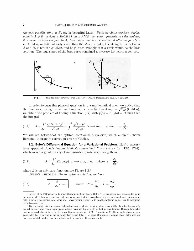
1.1. The Brachystochrone Problem. In 1696, Johann Bernoulli challenged themathematical world (which included his brother Jacob) with the following problem(see Figure 1.1): Given two fixed points A and B in a vertical plane, find a curveAMB such that a body gliding on it under gravity, starting from A, arrives after the
∗Received by the editors July 30, 2010; accepted for publication (in revised form) September 29,2011; published electronically November 8, 2012.
http://www.siam.org/journals/sirev/54-4/80403.html†Section de Mathematiques, Universite de Geneve, CP 64, 1211 Geneve (Martin.Gander@
unige.ch, [email protected]).
1
2 MARTIN J. GANDER AND GERHARD WANNER
shortest possible time at B, or, in beautiful Latin: Datis in plano verticali duobuspunctis A & B, assignare Mobili M viam AMB, per quam gravitate sua descendens,& moveri incipiens a puncto A, brevissimo tempore perveniat ad alterum punctumB. Galileo, in 1638, already knew that the shortest path, the straight line betweenA and B, is not the quickest, and he guessed wrongly that a circle would be the bestsolution. The true shape of the best curve remained a mystery for nearly a century.
dxdx
dydydsds
A
BM
x
y
Fig. 1.1 The brachystochrone problem (left); Jacob Bernoulli’s solution (right).
In order to turn this physical question into a mathematical one,1 we notice thatthe time for covering a small arc length ds is dJ = ds
v . Inserting v =√2gy (Galileo),
we obtain the problem of finding a function y(x) with y(a) = A, y(b) = B such thatthe integral
J =
∫ b
a
√dx2 + dy2√
2gy=
∫ b
a
√1 + p2√2gy
dx −→ min, where p =dy
dx.(1.1)
We will see below that the optimal solution is a cycloide, which allowed JohannBernoulli to proudly correct an error of Galileo.
1.2. Euler’s Differential Equation for a Variational Problem. Half a centurylater appeared Euler’s famous Methodus inveniendi lineas curvas [12] (E65, 1744),which solved a great variety of minimization problems, among them
J =
∫ b
a
Z(x, y, p) dx −→ min/max, where p =dy
dx,(1.2)
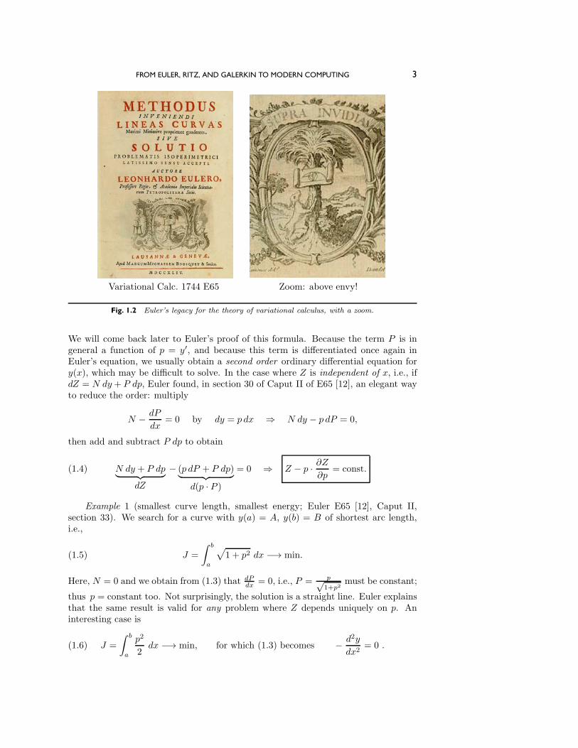
where Z is an arbitrary function; see Figure 1.2.2
Euler’s Theorem. For an optimal solution, we have
N − d
dxP = 0 , where N =
∂Z
∂y, P =
∂Z
∂p.(1.3)
1Letter of de l’Hopital to Johann Bernoulli, June 15th, 1696: “Ce probleme me paroist des pluscurieux et des plus jolis que l’on ait encore propose et je serois bien aise de m’y appliquer; mais pourcela il seroit necessaire que vous me l’envoyassiez reduit a la mathematique pure, car le phisiquem’embarasse . . . .”
2To represent his mathematical colleagues as dogs barking at a theory (the brachystochrone),nailed out of their reach high up on a tree, was not Euler’s style, but it was Johann Bernoulli’s, whohad produced the picture for his own Opera omnia in 1742. The editor, M. Bousquet, thought it agood idea to reuse the printing plate two years later. Perhaps Bousquet thought that Euler was anape sitting still higher up in the tree and eating up all the coconuts.
FROM EULER, RITZ, AND GALERKIN TO MODERN COMPUTING 3
Variational Calc. 1744 E65 Zoom: above envy!
Fig. 1.2 Euler’s legacy for the theory of variational calculus, with a zoom.
We will come back later to Euler’s proof of this formula. Because the term P is ingeneral a function of p = y′, and because this term is differentiated once again inEuler’s equation, we usually obtain a second order ordinary differential equation fory(x), which may be difficult to solve. In the case where Z is independent of x, i.e., ifdZ = N dy+ P dp, Euler found, in section 30 of Caput II of E65 [12], an elegant wayto reduce the order: multiply
N − dP
dx= 0 by dy = p dx ⇒ N dy − p dP = 0,
then add and subtract P dp to obtain
N dy + P dp︸ ︷︷ ︸dZ
− (p dP + P dp)︸ ︷︷ ︸d(p · P )
= 0 ⇒ Z − p · ∂Z∂p
= const.(1.4)
Example 1 (smallest curve length, smallest energy; Euler E65 [12], Caput II,section 33). We search for a curve with y(a) = A, y(b) = B of shortest arc length,i.e.,
J =
∫ b
a
√1 + p2 dx −→ min.(1.5)
Here, N = 0 and we obtain from (1.3) that dPdx = 0, i.e., P = p√
1+p2must be constant;
thus p = constant too. Not surprisingly, the solution is a straight line. Euler explainsthat the same result is valid for any problem where Z depends uniquely on p. Aninteresting case is
J =
∫ b
a
p2
2dx −→ min, for which (1.3) becomes − d2y
dx2= 0 .(1.6)
4 MARTIN J. GANDER AND GERHARD WANNER
This represents an approximation of J in (1.5) for small p and models a stretchedflexible cord. If a transversal force f(x) acts on the cord, we get the problem
J =
∫ b
a
(p2
2− f · y
)dx −→ min,
which leads to
−d2y
dx2= f(x) .
−1 1A B
y(x)
f(x)(1.7)
This case was too simple for Euler to mention, but its extension to higher dimensionswill become very important later.
Example 2 (the brachystochrone problem; Euler E65 [12], Caput II, section 34).We obtain from (1.4)√
1 + p2√2gy
− p2√2gy
√1 + p2
= C or 1 =√1 + p2
√2gy · C .(1.8)
It is still not a trivial matter to find a curve with this property. We remark thatJohann Bernoulli, with one of his typically brilliant intuitions, arrived immediately atthis last equation by applying Snell’s law of light refraction. Because sinα
v = const =1vdxds = 1/(
√1 + p2
√2gy), by (1.8) this law is satisfied everywhere and represents, by
Fermat’s principle, the quickest path.
1.3. Euler’s Integral Calculus. A considerable part of Euler’s tremendous workwas devoted to analytical and numerical methods for the solution of integrals anddifferential equations. This work culminated in the three volumes of InstitutionesCalculi Integralis [13] (E342, E366, E385, published 1768–1770). Let us apply thesemethods to find the solution of the brachystochrone problem (1.8): we solve theequation for p = dy
dx and obtain
1 + p2 =1
C2yor p =
dy
dx=
√1
C2y− 1 =
√c− y
y,(1.9)
with c = C−2. In section 397 of E342 [13], Euler explains that the variables x and yshould be separated, i.e.,√
y
c− y· dy = dx such that
∫ √y
c− y· dy = x .
The easiest method for such integrals are trigonometric substitutions, which Eulermentioned relatively late in E342 (in section 329). If we set y = c · sin2 u and profitfrom 1 − sin2 u = cos2 u, then the integral becomes an easy one and leads to thesolution
x = c u− c
2sin 2u, y = c · sin2 u =
c
2− c
2cos 2u ,
so that “curvam quaesitam esse Cycloidem.”Numerical Solution. Whenever such an analytical solution is not possible, Euler
proposed (in E342 [13], section 650) to compute the solution vero proxime assignare,by writing an equation such as (1.9) in the general form
dy
dx= V (x, y) , so that xi+1 = xi +Δx , yi+1 = yi +Δx · V (xi, yi)(1.10)
FROM EULER, RITZ, AND GALERKIN TO MODERN COMPUTING 5
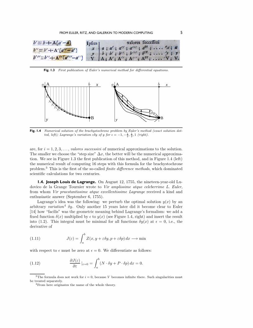
Fig. 1.3 First publication of Euler’s numerical method for differential equations.
y1
y2y3
y4 y5
A
B
x
y
ba A
B
x
y
δy
ba
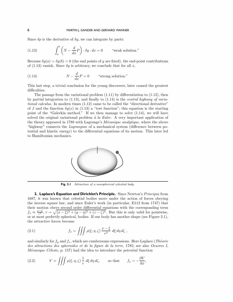
Fig. 1.4 Numerical solution of the brachystochrone problem by Euler’s method (exact solution dot-ted, left); Lagrange’s variation εδy of y for ε = −1,− 1
2, 12, 1 (right).
are, for i = 1, 2, 3, . . . , valores successivi of numerical approximations to the solution.The smaller we choose the “step size” Δx, the better will be the numerical approxima-tion. We see in Figure 1.3 the first publication of this method, and in Figure 1.4 (left)the numerical result of computing 16 steps with this formula for the brachystochroneproblem.3 This is the first of the so-called finite difference methods, which dominatedscientific calculations for two centuries.
1.4. Joseph Louis de Lagrange. On August 12, 1755, the nineteen-year-old Lu-dovico de la Grange Tournier wrote to Vir amplissime atque celeberrime L. Euler,from whom Vir praestantissime atque excellentissime Lagrange received a kind andenthusiastic answer (September 6, 1755).
Lagrange’s idea was the following: we perturb the optimal solution y(x) by anarbitrary variation4 δy. Only another 15 years later did it become clear to Euler[14] how “facilis” was the geometric meaning behind Lagrange’s formalism: we add afixed function δ(x) multiplied by ε to y(x) (see Figure 1.4, right) and insert the resultinto (1.2). This integral must be minimal for all functions δy(x) at ε = 0, i.e., thederivative of
J(ε) =
∫ b
a
Z(x, y + εδy, p+ εδp) dx −→ min(1.11)
with respect to ε must be zero at ε = 0. We differentiate as follows:
∂J(ε)
∂ε|ε=0 =
∫ b
a
(N · δy + P · δp) dx = 0.(1.12)
3The formula does not work for i = 0, because V becomes infinite there. Such singularities mustbe treated separately.
4From here originates the name of the whole theory.
6 MARTIN J. GANDER AND GERHARD WANNER
Since δp is the derivative of δy, we can integrate by parts:∫ b
a
(N − d
dxP
)· δy · dx = 0 “weak solution.”(1.13)
Because δy(a) = δy(b) = 0 (the end points of y are fixed), the end-point contributionsof (1.13) vanish. Since δy is arbitrary, we conclude that for all x,
N − d
dxP = 0 “strong solution.”(1.14)
This last step, a trivial conclusion for the young discoverer, later caused the greatestdifficulties.
The passage from the variational problem (1.11) by differentiation to (1.12), thenby partial integration to (1.13), and finally to (1.14) is the central highway of varia-tional calculus. In modern times (1.12) came to be called the “directional derivative”of J and the function δy(x) in (1.13) a “test function”; this equation is the startingpoint of the “Galerkin method.” If we then manage to solve (1.14), we will havesolved the original variational problem a la Euler. A very important application ofthe theory appeared in 1788 with Lagrange’s Mecanique analytique, where the above“highway” connects the Lagrangian of a mechanical system (difference between po-tential and kinetic energy) to the differential equations of its motion. This later ledto Hamiltonian mechanics.
Fig. 2.1 Attraction of a nonspherical celestial body.
2. Laplace’s Equation and Dirichlet’s Principle. Since Newton’s Principia from1687, it was known that celestial bodies move under the action of forces obeyingthe inverse square law, and since Euler’s work (in particular, E112 from 1747) thattheir motion obeys second order differential equations with the corresponding termfx ≈ x−ξ
r3 , r =√
(x− ξ)2 + (y − η)2 + (z − ζ)2. But this is only valid for pointwise,or at most perfectly spherical, bodies. If our body has another shape (see Figure 2.1),the attractive forces become
fx =
∫∫∫ρ(ξ, η, ζ)
x− ξ
r3dξ dη dζ ,(2.1)
and similarly for fy and fz, which are cumbersome expressions. Here Laplace (Theoriedes attractions des spheroides et de la figure de la terre, 1785; see also Oeuvres I,Mecanique Celeste, p. 157) had the idea to introduce the potential function
V =
∫∫∫ρ(ξ, η, ζ)
1
rdξ dη dζ, so that fx = −∂V
∂x,(2.2)
FROM EULER, RITZ, AND GALERKIN TO MODERN COMPUTING 7
and similarly for fy and fz. If we differentiate (2.1) once again with respect to x (andy and z, respectively), we find for V the elegant expression
ΔV =∂2V
∂x2+∂2V
∂y2+∂2V
∂z2= 0,(2.3)
which bears the name Laplace’s equation.Soon after its formulation, this equation found many other important applications,
not only in the heavens, but also down on earth:• theory of stationary heat transfer (Fourier, 1822);• theory of magnetism (Gauss and Weber in Gottingen, C.F.Gauss, Werke 5,p. 195, 1839 [16]);
• theory of electric fields (W.Thomson, later Lord Kelvin [44], 1847);• conformal mappings (Gauss, Werke IV, p. 189, 1825);• in complex analysis (Cauchy, 1825, and Riemann [36], Thesis, 1851);• irrotational fluid motion in two dimensions (Helmholtz, 1858).
All these applications led young Riemann to the following enthusiastic statement:
. . . eine vollkommen in sich abgeschlossene mathematische Theorie . . . ,
welche . . . fortschreitet, ohne zu scheiden, ob es sich um die Schwerkraft,
oder die Electricitat, oder den Magnetismus, oder das Gleichgewicht der
Warme handelt. (Manuscript of Riemann, Nov. 1850, Werke, p. 545.)
2.1. Conformal Maps and the Riemann Mapping Theorem. In his thesis [36]from 1851, Riemann founded geometric function theory, which studies theorems incomplex analysis through elegant geometric considerations, and which was later per-fected mainly through the work of Richard Courant (cf. the second part of Hurwitzand Courant [24]). The starting points are the Cauchy–Riemann differential equationsfor continuously differentiable functions f(z) = u(x, y) + iv(x, y) with z = x+ iy,
(2.4)
in Riemann’s handwriting,5 which, when differentiated, give
Δu =∂2u
∂x2+∂2u
∂y2= 0 and Δv =
∂2v
∂x2+∂2v
∂y2= 0,(2.5)
i.e., u and v are harmonic. Furthermore, equations (2.4) tell us that the Jacobian inR
2 of a continuously differentiable function is of the form( ∂u∂x
∂u∂y
∂v∂x
∂v∂y
)=
(a b−b a
)= Const ·
(cosφ sinφ− sinφ cosφ
),(2.6)
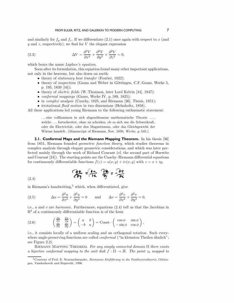
i.e., it consists locally of a uniform scaling and an orthogonal rotation. Such every-where angle-preserving functions are called conformal (“in kleinsten Theilen ahnlich”;see Figure 2.2).
Riemann Mapping Theorem. For any simply connected domain Ω there existsa bijective conformal mapping to the unit disk f : Ω → B. The point z0 mapped to
5Courtesy of Prof. E. Neuenschwander, Riemanns Einfuhrung in die Funktionentheorie, Gottin-gen, Vandenhoeck and Ruprecht, 1996.
8 MARTIN J. GANDER AND GERHARD WANNER
zz
H
α1z1
α2α3
α4z4
α5z5
α6
α7
α8
w = f(z)w = f(z)
f(H)
α1w1
α2
α3
α4w4
α5w5
α6
α7
α8
Fig. 2.2 A conformal mapping.
−→f
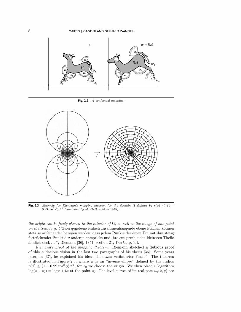
Fig. 2.3 Example for Riemann’s mapping theorem for the domain Ω defined by r(φ) ≤ (1 −0.99 cos2 φ)1/2 (computed by M. Gutknecht in 1975).
the origin can be freely chosen in the interior of Ω, as well as the image of one pointon the boundary. (“Zwei gegebene einfach zusammenhangende ebene Flachen konnenstets so aufeinander bezogen werden, dass jedem Punkte der einen Ein mit ihm stetigfortruckender Punkt der anderen entspricht und ihre entsprechenden kleinsten Theileahnlich sind; . . . ”; Riemann [36], 1851, section 21, Werke, p. 40).
Riemann’s proof of the mapping theorem. Riemann sketched a dubious proofof this audacious vision in the last two paragraphs of his thesis [36]. Some yearslater, in [37], he explained his ideas “in etwas veranderter Form.” The theoremis illustrated in Figure 2.3, where Ω is an “inverse ellipse” defined by the radiusr(φ) ≤ (1 − 0.99 cos2 φ)1/2; for z0 we choose the origin. We then place a logarithmlog(z − z0) = log r + iφ at the point z0. The level curves of its real part u0(x, y) are
FROM EULER, RITZ, AND GALERKIN TO MODERN COMPUTING 9
the concentric circles around z0; the level curves of the imaginary part, orthogonal tothe first ones, are the star-shaped rays out of z0. The problem is that the boundaryof Ω is normally not a level curve of u0. We postulate that there exists an everywhereharmonic function u1(x, y) such that u1(x, y) = u0(x, y) on the boundary ∂Ω. Thefunction u(x, y) := u0(x, y) − u1(x, y) will be harmonic in Ω with the exception ofthe point z0, where we have the logarithmic singularity, and it will be zero on ∂Ω.By solving the differential equations (2.4), we complete u(x, y) to a complex functionu(x, y) + iv(x, y). The exponential function of this function will then map z0 to theorigin and the boundary of Ω to the boundary of the circle.
These ideas of Riemann left scientists with much to do over the next century:clarifying the above proof, clarifying regularity conditions, developing the theory formore general domains, and developing better computational algorithms; see the lastchapter of [24], Chapters 16 and 17 of Henrici’s trilogy [20], and Gutknecht [19]. Themain obstacle was the existence of the function u1, which we will discuss in the nextsubsection.
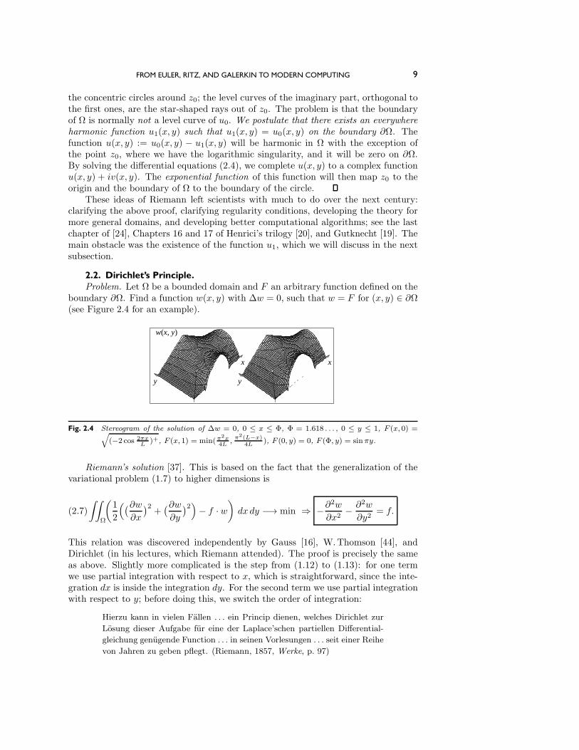
2.2. Dirichlet’s Principle.Problem. Let Ω be a bounded domain and F an arbitrary function defined on the
boundary ∂Ω. Find a function w(x, y) with Δw = 0, such that w = F for (x, y) ∈ ∂Ω(see Figure 2.4 for an example).
xxxx
yyyy
w(x, y)
Fig. 2.4 Stereogram of the solution of Δw = 0, 0 ≤ x ≤ Φ, Φ = 1.618 . . . , 0 ≤ y ≤ 1, F (x, 0) =√(−2 cos 2πx
L)+, F (x, 1) = min(π
2x4L
,π2(L−x)
4L), F (0, y) = 0, F (Φ, y) = sinπy.
Riemann’s solution [37]. This is based on the fact that the generalization of thevariational problem (1.7) to higher dimensions is
∫∫Ω
(1
2
((∂w∂x
)2+(∂w∂y
)2)− f · w)dx dy −→ min ⇒ −∂
2w
∂x2− ∂2w
∂y2= f.(2.7)
This relation was discovered independently by Gauss [16], W.Thomson [44], andDirichlet (in his lectures, which Riemann attended). The proof is precisely the sameas above. Slightly more complicated is the step from (1.12) to (1.13): for one termwe use partial integration with respect to x, which is straightforward, since the inte-gration dx is inside the integration dy. For the second term we use partial integrationwith respect to y; before doing this, we switch the order of integration:
Hierzu kann in vielen Fallen . . . ein Princip dienen, welches Dirichlet zur
Losung dieser Aufgabe fur eine der Laplace’schen partiellen Differential-
gleichung genugende Function . . . in seinen Vorlesungen . . . seit einer Reihe
von Jahren zu geben pflegt. (Riemann, 1857, Werke, p. 97)
10 MARTIN J. GANDER AND GERHARD WANNER
Riemann concludes that for all functions defined on Ω with the prescribed boundaryvalues F , the integral
J(w) =
∫∫Ω
1
2
((∂w∂x
)2+(∂w∂y
)2)dx dy is always > 0.(2.8)
Choose among these functions the one for which this integral has the smallest possiblevalue!
In other words, we pass through the Euler–Lagrange highway (1.11) ⇒ (1.14) inthe opposite direction (1.11)⇐ (1.14). In contrast to “Euler’s world,” here the solutionof the differential equation (1.14) is impossible, whereas the variational problem (1.11)appears “trivial.” From here originate the terms “Dirichlet’s principle” and “Dirichletboundary conditions.”
Weierstrass’s Critique. Soon afterwards some people started to mistrust this“brave new world,” the most serious critic being Weierstrass [49] with the counterex-ample ∫ 1
−1
(x · y′)2 dx −→ min
y(−1) = a, y(1) = b
y = a+b2 + b−a
2
arctan xε
arctan 1ε
−1 0 1a
b
.(2.9)
The factor x in the integral allows y′ to do anything close to the origin, and the solutionof the problem becomes discontinuous (“Die Dirichlet’sche Schlussweise fuhrt also indem betrachteten Falle offenbar zu einem falschen Resultat.”)
F.Klein (Entw. Math., 19, Jahrh., Chelsea, 1967, p. 264) reports that Riemannreplied to Weierstrass, “my theorems remain nevertheless true” (“meine Existenz-theoreme sind trotzdem richtig”), and that Helmholtz declared “for us physicistsDirichlet’s principle remains a proof” (“fur uns Physiker bleibt das DirichletschePrinzip ein Beweis”).
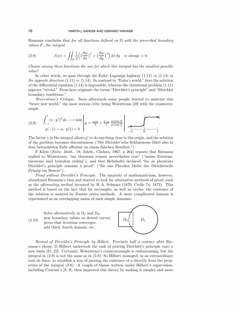
Proof without Dirichlet’s Principle. The majority of mathematicians, however,abandoned Riemann’s idea and started to look for alternative methods of proof, suchas the alternating method invented by H.A. Schwarz (1870, Crelle 74, 1872). Thismethod is based on the fact that for rectangles, as well as circles, the existence ofthe solution is assured by Fourier series methods. A more complicated domain isrepresented as an overlapping union of such simple domains:
Solve alternatively in Ω1 and Ω2;new boundary values on dotted curves;prove that iteration converges;add third, fourth domain, etc.
Ω1Ω2(2.10)
Revival of Dirichlet’s Principle by Hilbert. Precisely half a century after Rie-mann’s thesis, D. Hilbert undertook the task of putting Dirichlet’s principle onto anew basis [21, 22]. Certainly, Weierstrass’s counterexample is embarrassing, but theintegral in (2.9) is not the same as in (2.8). So Hilbert managed, in an extraordinarytour de force, to establish a way of proving the existence of u directly from the prop-erties of the integral (2.8). A couple of theses written under Hilbert’s supervision,including Courant’s [8, 9], then improved this theory by making it simpler and more
FROM EULER, RITZ, AND GALERKIN TO MODERN COMPUTING 11
complete. These discussions became another motivation for W.Ritz to develop hismethod.
Das Dirichletsche Prinzip verdankte seinen Ruhm der anziehenden Ein-
fachheit seiner mathematischen Grundidee, dem unleugbaren Reichtum
der moglichen Anwendungen . . . und der ihm innewohnenden Uberzeugungskraft.
(D.Hilbert)
Mittlerweile war das verachtete und scheintote Dirichletsche Prinzip durch
Hilbert wieder zum Leben erweckt worden; . . . (Hurwitz and Courant [24,
p. 392])
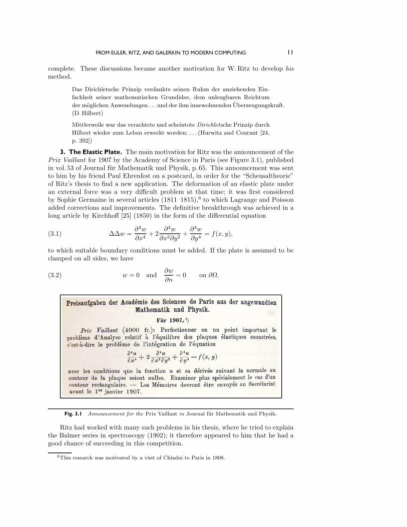
3. The Elastic Plate. The main motivation for Ritz was the announcement of thePrix Vaillant for 1907 by the Academy of Science in Paris (see Figure 3.1), publishedin vol. 53 of Journal fur Mathematik und Physik, p. 65. This announcement was sentto him by his friend Paul Ehrenfest on a postcard, in order for the “Scheusaltheorie”of Ritz’s thesis to find a new application. The deformation of an elastic plate underan external force was a very difficult problem at that time; it was first consideredby Sophie Germaine in several articles (1811–1815),6 to which Lagrange and Poissonadded corrections and improvements. The definitive breakthrough was achieved in along article by Kirchhoff [25] (1850) in the form of the differential equation
ΔΔw =∂4w
∂x4+ 2
∂4w
∂x2∂y2+∂4w
∂y4= f(x, y),(3.1)
to which suitable boundary conditions must be added. If the plate is assumed to beclamped on all sides, we have
w = 0 and∂w
∂n= 0 on ∂Ω.(3.2)
Fig. 3.1 Announcement for the Prix Vaillant in Journal fur Mathematik und Physik.
Ritz had worked with many such problems in his thesis, where he tried to explainthe Balmer series in spectroscopy (1902); it therefore appeared to him that he had agood chance of succeeding in this competition.
6This research was motivated by a visit of Chladni to Paris in 1808.
12 MARTIN J. GANDER AND GERHARD WANNER
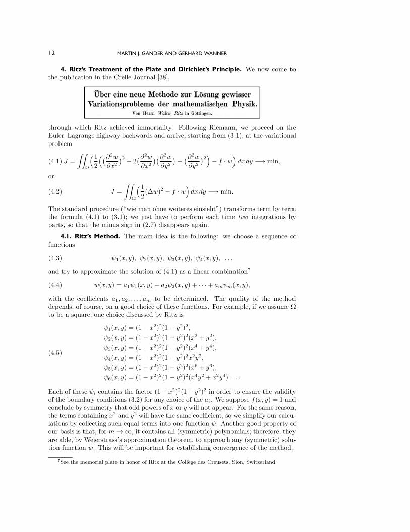
4. Ritz’s Treatment of the Plate and Dirichlet’s Principle. We now come tothe publication in the Crelle Journal [38],
through which Ritz achieved immortality. Following Riemann, we proceed on theEuler–Lagrange highway backwards and arrive, starting from (3.1), at the variationalproblem
J =
∫∫Ω
(12
((∂2w∂x2
)2+ 2
(∂2w∂x2
)(∂2w∂y2
)+(∂2w∂y2
)2)− f · w)dx dy −→ min,(4.1)
or
J =
∫∫Ω
(12(Δw)2 − f · w
)dx dy −→ min.(4.2)
The standard procedure (“wie man ohne weiteres einsieht”) transforms term by termthe formula (4.1) to (3.1); we just have to perform each time two integrations byparts, so that the minus sign in (2.7) disappears again.
4.1. Ritz’s Method. The main idea is the following: we choose a sequence offunctions
ψ1(x, y), ψ2(x, y), ψ3(x, y), ψ4(x, y), . . .(4.3)
and try to approximate the solution of (4.1) as a linear combination7
w(x, y) = a1ψ1(x, y) + a2ψ2(x, y) + · · ·+ amψm(x, y),(4.4)
with the coefficients a1, a2, . . . , am to be determined. The quality of the methoddepends, of course, on a good choice of these functions. For example, if we assume Ωto be a square, one choice discussed by Ritz is
ψ1(x, y) = (1− x2)2(1 − y2)2,
ψ2(x, y) = (1− x2)2(1 − y2)2(x2 + y2),
ψ3(x, y) = (1− x2)2(1 − y2)2(x4 + y4),
ψ4(x, y) = (1− x2)2(1 − y2)2x2y2,
ψ5(x, y) = (1− x2)2(1 − y2)2(x6 + y6),
ψ6(x, y) = (1− x2)2(1 − y2)2(x4y2 + x2y4) . . . .
(4.5)
Each of these ψi contains the factor (1− x2)2(1− y2)2 in order to ensure the validityof the boundary conditions (3.2) for any choice of the ai. We suppose f(x, y) = 1 andconclude by symmetry that odd powers of x or y will not appear. For the same reason,the terms containing x2 and y2 will have the same coefficient, so we simplify our calcu-lations by collecting such equal terms into one function ψ. Another good property ofour basis is that, for m→ ∞, it contains all (symmetric) polynomials; therefore, theyare able, by Weierstrass’s approximation theorem, to approach any (symmetric) solu-tion function w. This will be important for establishing convergence of the method.
7See the memorial plate in honor of Ritz at the College des Creusets, Sion, Switzerland.
FROM EULER, RITZ, AND GALERKIN TO MODERN COMPUTING 13
If we insert the expression (4.4) into (4.2), we obtain a finite-dimensional expres-sion in a1, a2, . . . , am. By chance, J in (4.2) contains only quadratic and linear termsof w. Hence, if we multiply out all the terms, we obtain a finite-dimensional quadraticfunction
Jm =1
2
m∑i,j=1
kijaiaj −m∑i=1
biai,(4.6)
with
kij =
∫ 1
−1
∫ 1
−1
Δψi ·Δψj dx dy , bi =
∫ 1
−1
∫ 1
−1
ψi · f dx dy .(4.7)
Differentiating (4.6) with respect to a�, for � = 1, 2, . . . ,m, we find that Jm is minimalif
m∑j=1
k�jaj = b� .(4.8)
This is a linear system which, in theory, is easily solvable. In practice, however, thesystem is very tedious to solve: for m = 6, obtaining just one of the 21 k-values wouldrequire us to compute
Δψ6 ·Δψ6 = 8 x2(1− y2
)2 (x4y2 + x2y4
)− 8
(1− x2
) (1− y2
)2 (4 x3y2 + 2 xy4
)x
− 4(1− x2
) (1− y2
)2 (x4y2 + x2y4
)+(1− x2
)2 (1− y2
)2 (12 x2y2 + 2 y4
)+ 8
(1− x2
)2y2(x4y2 + x2y4
)− 8
(1− x2
)2 (1− y2
) (2 x4y + 4 x2y3
)y
− 4(1− x2
)2 (1− y2
) (x4y2 + x2y4
)+(1− x2
)2 (1− y2
)2 (2 x4 + 12 x2y2
)and then
∫ 1
−1
∫ 1
−1 Δψ6 ·Δψ6 dx dy = 30524047366898776885 . We can understand why Ritz did not
use this particular basis to demonstrate his method numerically. We, however, havemodern computers and find the system
53.49878 9.72705 2.13385 0.54039 0.63739 0.30484 1.137789.72705 21.94822 10.91868 1.74588 5.99358 1.25965 0.325082.13385 10.91868 9.63314 0.90947 7.10042 1.01770 0.108360.54039 1.74588 0.90947 0.47237 0.51468 0.39553 0.023220.63739 5.99358 7.10042 0.51468 6.32258 0.73117 0.049250.30484 1.25965 1.01770 0.39553 0.73117 0.44246 0.01548
(4.9)
If we set m = 1, only k11a1 = b1 has to be considered and we obtain by a simpledivision
a1 = 1.13778/53.49878 = 0.021267.(4.10)
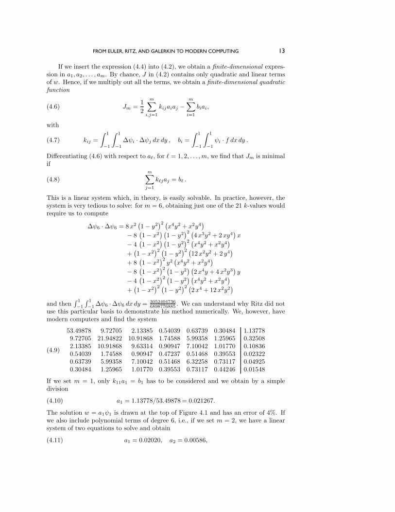
The solution w = a1ψ1 is drawn at the top of Figure 4.1 and has an error of 4%. Ifwe also include polynomial terms of degree 6, i.e., if we set m = 2, we have a linearsystem of two equations to solve and obtain
a1 = 0.02020, a2 = 0.00586,(4.11)
14 MARTIN J. GANDER AND GERHARD WANNER
xxxx
yyyy
w1(x, y)
xxxx
yyyy
w2(x, y)
m = 1, errmax= 0.04
m = 2, errmax= 0.003
Fig. 4.1 Solutions of the plate problem for m = 1 and m = 2.
0 1 0 1 0 1 0 1
ξ1 ξ2 ξ3 ξ4
Fig. 4.2 One-dimensional elastic curves.
which reduces the error to 0.3% (bottom of Figure 4.1). Taking into account also8th-degree terms (m = 4) leads to a relative error of 10−5 with precisely the samegraphical representation as for m = 2. For m = 6 the solutions are
a1 = 0.02025, a2 = 0.00521, a3 = 0.00028,a4 = 0.00612, a5 = −0.00002, a6 = 0.00012 .
(4.12)
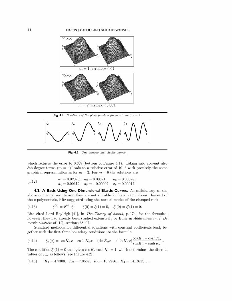
4.2. A Basis Using One-Dimensional Elastic Curves. As satisfactory as theabove numerical results are, they are not suitable for hand calculations. Instead ofthese polynomials, Ritz suggested using the normal modes of the clamped rod:
ξ(4) = K4 · ξ, ξ(0) = ξ(1) = 0, ξ′(0) = ξ′(1) = 0.(4.13)
Ritz cited Lord Rayleigh [41], in The Theory of Sound, p. 174, for the formulas;however, they had already been studied extensively by Euler in Additamentum I, Decurvis elasticis of [12], sections 68–97.
Standard methods for differential equations with constant coefficients lead, to-gether with the first three boundary conditions, to the formula
ξn(x) = cosKnx− coshKnx− (sinKnx− sinhKnx)cosKn − coshKn
sinKn − sinhKn.(4.14)
The condition ξ′(1) = 0 then gives cosKn coshKn = 1, which determines the discretevalues of Kn as follows (see Figure 4.2):
K1 = 4.7300, K2 = 7.8532, K3 = 10.9956, K4 = 14.1372, . . . .(4.15)
FROM EULER, RITZ, AND GALERKIN TO MODERN COMPUTING 15
Because coshK tends to infinity very rapidly, Kn will also quickly approach the rootsof the cosine, i.e., Kn ≈ (n+ 1
2 )π.Taking into account again the symmetry of the solution, we use the basis
ψ1(x, y) = ξ1(x)ξ1(y), ψ2(x, y) = ξ1(x)ξ3(y) + ξ3(x)ξ1(y),
ψ3(x, y) = ξ3(x)ξ3(y), ψ4(x, y) = ξ1(x)ξ5(y) + ξ5(x)ξ1(y), . . . .
The advantages of this basis are that1. we only have one defining formula (4.14) for every n;2. using integration by parts, the condition (4.13) leads to easy formulas for the
integrals (4.7); and3. the linear system (4.8) becomes strongly diagonally dominant.
It can thus be solved easily (“der Rechenschieber angewandt werden kann. . .”) by asort of “Gauss–Seidel” iteration. (“Eine direkte Losung durch Determinanten wurde5stellige Logarithmentafeln erfordern.”) In this way, Ritz obtained the solutions
w1(x, y) = 0.6620ξ1(x)ξ1(y),
w2(x, y) = 0.6727ξ1(x)ξ1(y) + 0.0307(ξ1(x)ξ3(y)+ ξ3(x)ξ1(y)) + 0.0031ξ3(x)ξ3(y),
w3(x, y) = 0.6740ξ1(x)ξ1(y) + 0.0380(ξ1(x)ξ3(y) + ξ3(x)ξ1(y))+ 0.0032ξ3(x)ξ3(y) + 0.0040(ξ1(x)ξ5(y) + ξ5(x)ξ1(y))+ 0.0004(ξ3(x)ξ5(y) + ξ5(x)ξ3(y)) + 0.0000ξ5(x)ξ5(y),
whose graphical representation is not so different from those in Figure 4.1.Theorem of Existence and Convergence. Based on• a careful study of speed of convergence based on the asymptotic values of Kn,allowing the exchange of differentiations and limits;
• Weierstrass’s approximation theorem; and• a modification of a lemma from Hilbert’s proof (1901),
Ritz managed, in paragraphs 3, 4, and 5 of his paper, to prove rigorously that thewm(x, y) converge to a function w(x, y) that solves the minimization problem.
4.3. Dirichlet’s Principle. In the second part of [38], Ritz applied his proofs toDirichlet’s problem (see section 2.2)
Δw = 0, w|∂Ω = F .
In order to have the boundary values equal to 0, we subtract F from w and obtain aproblem of the type
−Δw = f, w|∂Ω = 0 .(4.16)
16 MARTIN J. GANDER AND GERHARD WANNER
xxxx
yyyy
w1(x, y)
xxxx
yyyy
w2(x, y)
m = 1, errmax= 0.05
m = 2, errmax= 0.01
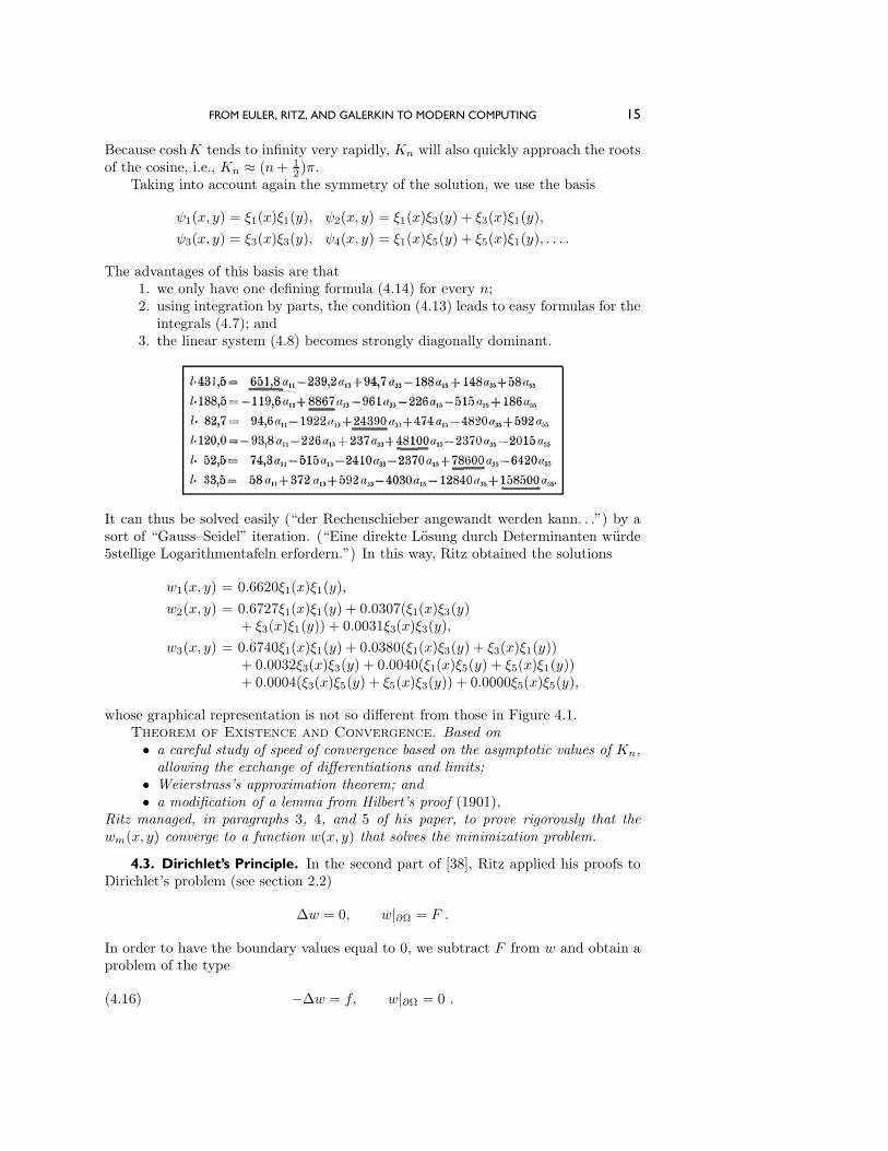
Fig. 4.3 Solutions for Dirichlet’s principle.
Inserting (4.4) into (2.7), we obtain
kij=
∫ 1
−1
∫ 1
−1
(∂ψi
∂x
∂ψj
∂x+∂ψi
∂y
∂ψj
∂y
)dx dy , bi =
∫ 1
−1
∫ 1
−1
ψi · f dx dy,(4.17)
instead of (4.7). Ritz then proceeded to prove once again the existence and conver-gence of his method, but he did not show numerical examples; for the square theywould have been too simple.
Let us show them here, by modifying the basis functions according to the newboundary condition as
ψ1(x, y) = (1− x2)(1 − y2),
ψ2(x, y) = (1− x2)(1 − y2)(x2 + y2),
ψ3(x, y) = (1− x2)(1 − y2)(x4 + y4),
ψ4(x, y) = (1− x2)(1 − y2)x2y2,
ψ5(x, y) = (1− x2)(1 − y2)(x6 + y6),
ψ6(x, y) = (1− x2)(1 − y2)(x4y2 + x2y4) . . . ,
and obtain, proceeding as above, the solutions
for m = 1 : a1 = 0.3125;
for m = 2 : a1 = 0.2922, a2 = 0.05923 .(4.18)
These solutions are drawn in Figure 4.3. Again, the higher order terms have little effecton the graphic representation of the function. One observes that for each increase ofthe degree by a factor of 2, the error decreases by a factor of 4.
5. Ritz Computes Chladni Figures. In 1787, Ernst Florence Friedrich Chladni,a musician and physicist from Wittenberg close to Leipzig, made an extraordinarydiscovery [5]: he noticed that when he tried to excite a metal plate with the bow ofhis violin, he could make sounds of different pitch, depending on where he touched the
FROM EULER, RITZ, AND GALERKIN TO MODERN COMPUTING 17
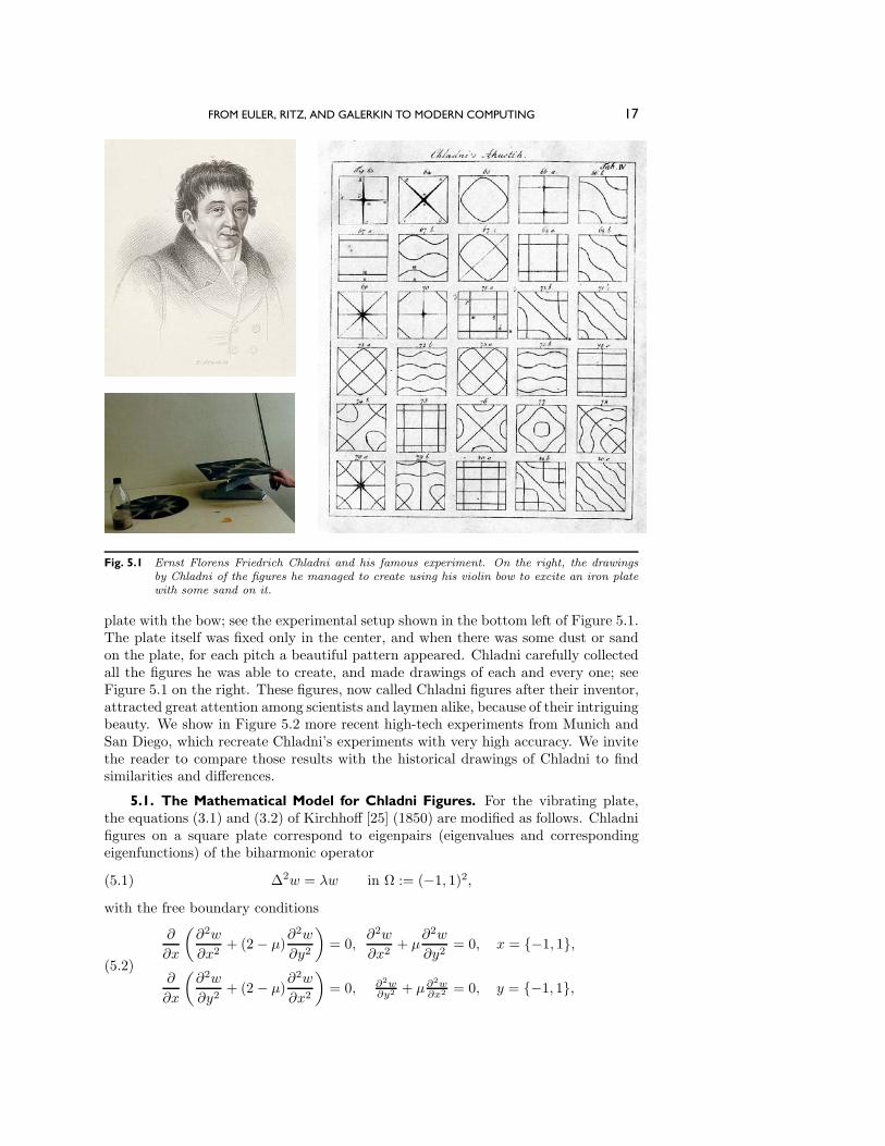
Fig. 5.1 Ernst Florens Friedrich Chladni and his famous experiment. On the right, the drawingsby Chladni of the figures he managed to create using his violin bow to excite an iron platewith some sand on it.
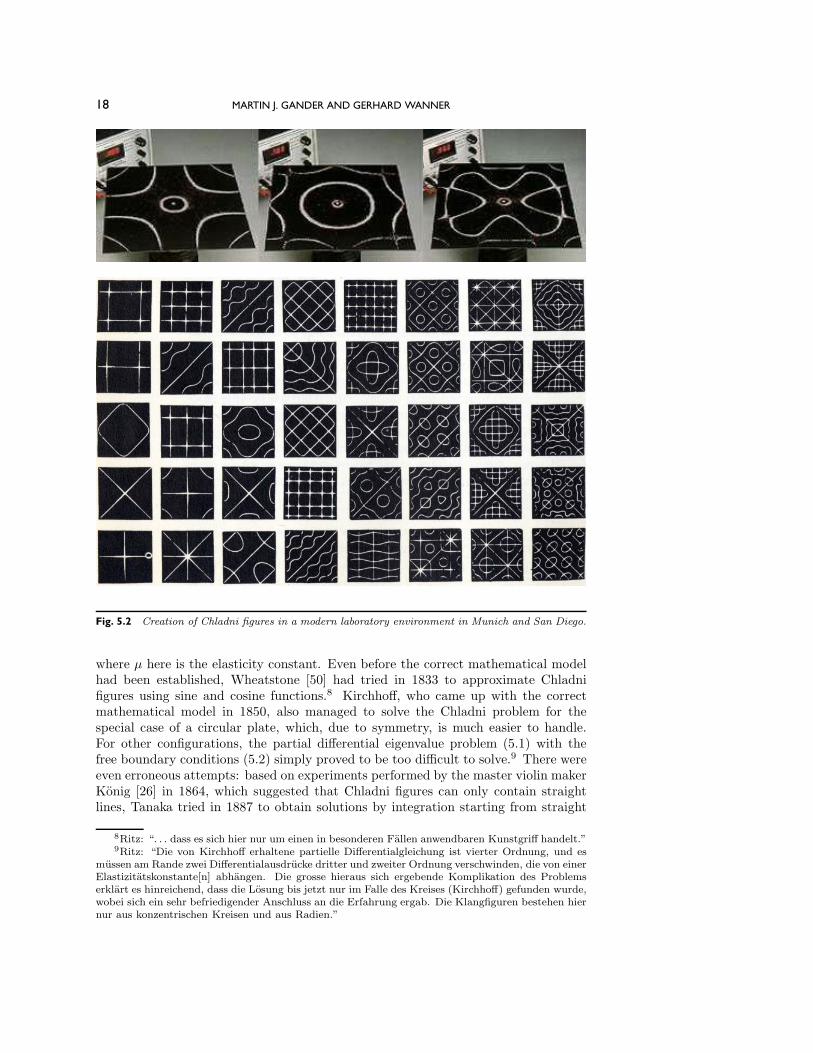
plate with the bow; see the experimental setup shown in the bottom left of Figure 5.1.The plate itself was fixed only in the center, and when there was some dust or sandon the plate, for each pitch a beautiful pattern appeared. Chladni carefully collectedall the figures he was able to create, and made drawings of each and every one; seeFigure 5.1 on the right. These figures, now called Chladni figures after their inventor,attracted great attention among scientists and laymen alike, because of their intriguingbeauty. We show in Figure 5.2 more recent high-tech experiments from Munich andSan Diego, which recreate Chladni’s experiments with very high accuracy. We invitethe reader to compare those results with the historical drawings of Chladni to findsimilarities and differences.
5.1. The Mathematical Model for Chladni Figures. For the vibrating plate,the equations (3.1) and (3.2) of Kirchhoff [25] (1850) are modified as follows. Chladnifigures on a square plate correspond to eigenpairs (eigenvalues and correspondingeigenfunctions) of the biharmonic operator
Δ2w = λw in Ω := (−1, 1)2,(5.1)
with the free boundary conditions
∂
∂x
(∂2w
∂x2+ (2 − μ)
∂2w
∂y2
)= 0,
∂2w
∂x2+ μ
∂2w
∂y2= 0, x = {−1, 1},
∂
∂x
(∂2w
∂y2+ (2 − μ)
∂2w
∂x2
)= 0, ∂2w
∂y2 + μ∂2w∂x2 = 0, y = {−1, 1},
(5.2)
18 MARTIN J. GANDER AND GERHARD WANNER
Fig. 5.2 Creation of Chladni figures in a modern laboratory environment in Munich and San Diego.
where μ here is the elasticity constant. Even before the correct mathematical modelhad been established, Wheatstone [50] had tried in 1833 to approximate Chladnifigures using sine and cosine functions.8 Kirchhoff, who came up with the correctmathematical model in 1850, also managed to solve the Chladni problem for thespecial case of a circular plate, which, due to symmetry, is much easier to handle.For other configurations, the partial differential eigenvalue problem (5.1) with thefree boundary conditions (5.2) simply proved to be too difficult to solve.9 There wereeven erroneous attempts: based on experiments performed by the master violin makerKonig [26] in 1864, which suggested that Chladni figures can only contain straightlines, Tanaka tried in 1887 to obtain solutions by integration starting from straight
8Ritz: “. . . dass es sich hier nur um einen in besonderen Fallen anwendbaren Kunstgriff handelt.”9Ritz: “Die von Kirchhoff erhaltene partielle Differentialgleichung ist vierter Ordnung, und es
mussen am Rande zwei Differentialausdrucke dritter und zweiter Ordnung verschwinden, die von einerElastizitatskonstante[n] abhangen. Die grosse hieraus sich ergebende Komplikation des Problemserklart es hinreichend, dass die Losung bis jetzt nur im Falle des Kreises (Kirchhoff) gefunden wurde,wobei sich ein sehr befriedigender Anschluss an die Erfahrung ergab. Die Klangfiguren bestehen hiernur aus konzentrischen Kreisen und aus Radien.”
FROM EULER, RITZ, AND GALERKIN TO MODERN COMPUTING 19
lines.10 In the case of clamped boundaries, the problem greatly simplifies, and Voigt[48] found the general solution in 1893 for a rectangular plate with two or four clampedboundaries by elementary integration. Toward the end of the 19th century, the greatexpert in sound, John William Strutt, later Baron Rayleigh, summarized the situationin [41]: “The Problem of a rectangular plate, whose edges are free, is one of greatdifficulty, and has for the most part resisted attack.”
5.2. Ritz’s Computation of Chladni Figures. In his second groundbreaking pa-per [39], Walther Ritz presents and analyzes his own method in order to computeChladni figures: instead of trying to solve the partial differential eigenvalue problem(5.1)–(5.2) directly, he proposes to use the principle of energy minimization, fromwhich the equations were derived,11 and thus he considers the functional
J(w) :=
∫ 1
−1
∫ 1
−1
[(∂2w
∂x2
)2
+
(∂2w
∂y2
)2
+ 2μ∂2w
∂x2∂2w
∂y2+ 2(1− μ)
(∂2w
∂x∂y
)2].(5.3)
According to the minimization principle, the solution w of (5.1)–(5.2) is a minimumof the constrained problem
J(w) → min,
∫ 1
−1
∫ 1
−1
w2 dx dy = const.,(5.4)
and, from this minimization problem, one can again obtain the partial differentialeigenvalue problem by simply using the central highway of variational calculus.
Even though Ritz explains his new method using the concrete example of Chladnifigures on a square plate, he points out that his new method is completely general andcould be applied to plates of arbitrary shapes, provided the basis functions are wellchosen.12 The fundamental idea of Ritz’s new method was to search for an approx-imate solution of the problem as a combination of well-chosen so-called coordinatefunctions (“Grundfunktionen”) of the form
ws =
s∑m=0
Amwm(x, y).(5.5)
If a simple solution is sought, for example, the lowest pitch, Ritz points out thatone could simply choose polynomials for the basis functions wm(x, y).13 For highereigenmodes, a better choice that leads to more accuracy is to use the same coordinate
10Ritz: “. . . Tanaka glaubt, allgemeinere und strengere Formeln zu erhalten. Dies ist aber schondeswegen nicht der Fall, weil ubersehen ist, dass eine Randbedingung die Losung gar nicht bestimmt.”
11Ritz: “Das wesentliche der neuen Methode besteht darin, dass nicht von den Differentialgle-ichungen und Randbedingungen des Problems, sondern direkt vom Prinzip der kleinsten Wirkungausgegangen wird, aus welchem ja durch Variation jene Gleichungen und Bedingungen gewonnenwerden konnen.”
12Ritz: “Im folgenden entwickle ich am Beispiel der quadratischen Platten mit freien Randern eineneue Integrationsmethode, die ohne wesentliche Anderungen auch auf rechteckige Platten angewandtwerden kann, sei es mit freien, sei es auch mit teilweise oder ganz eingespannten oder gestutztenRandern. Theoretisch ist die Losung in ahnlicher Weise sogar fur eine beliebige Gestalt der Plattemoglich; eine genaue Berechnung einer grosseren Anzahl von Klangfiguren, wie sie im folgenden furden klassischen Fall der quadratischen Scheibe durchgefuhrt ist, wird aber nur bei geeigneter Wahlder Grundfunktionen, nach welchen entwickelt wird, praktisch ausfuhrbar.”
13Ritz: “Fur den Grundton, wofern grosse Genauigkeit nicht gefordert wird, fuhrt das Verfahrenfur die meisten Platten durch den Ansatz von Polynomen zum Ziel.”

20 MARTIN J. GANDER AND GERHARD WANNER
functions as in the previous section:14
wmn = um(x)un(y) + um(y)un(x),
w′mn = um(x)un(y)− um(y)un(x),
where um(x) are the known eigenfunctions of a free one-dimensional bar,
d4umdx4
= k4mum, withd2umdx2
= 0,d3umdx3
= 0 at x = {−1, 1}.
These conditions lead to the functions
um =
⎧⎪⎨⎪⎩cosh km cos kmx+cos km cosh kmx√
cosh2 km+cos2 km
, tan km + tanh km = 0, m even,
sinh km sin kmx+sin km sinhkmx√sinh2 km−sin2 km
, tan km − tanhkm = 0, m odd.(5.6)
Ritz approximation of the solution then takes the form
ws :=
s∑m=0
s∑n=0
Amnum(x)un(y).(5.7)
In order to determine the coefficients Amn, we again insert this solution into thefunctional (5.3), and we require that the resulting functional∫ 1
−1
∫ 1
−1
[(∂2ws
∂x2
)2
+
(∂2ws
∂y2
)2
+ 2μ∂2ws
∂x2∂2ws
∂y2+ 2(1− μ)
(∂2ws
∂x∂y
)2]dx dy(5.8)
is minimal15 under the constraint
U(ws) :=
∫ 1
−1
∫ 1
−1
w2s dx dy = const. =: C.(5.9)
In this approximate problem, we only need to determine a finite number of coefficientsAmn.
In order to express the functional J(ws) in terms of the coefficients Amn, we haveto evaluate several integral terms. The first one is
∫ 1
−1
∫ 1
−1
(∂2ws
∂x2
)2dx dy =
∫ 1
−1
∫ 1
−1
(∂2∑
m,nAmnum(x)un(y)
∂x2
)2
dx dy
=∑m,n
∑p,q
AmnApq
∫ 1
−1
∫ 1
−1
∂2um(x)
∂x2un(y)
∂2up(x)
∂x2uq(y) dx dy︸ ︷︷ ︸
c1mnpq:=
.(5.10)
Since un is known, it suffices to evaluate the integrals numerically to obtain thecoefficients c1mnpq. Similarly, one can also evaluate all the other terms in (5.8) to
14Ritz: “Samtliche Eigentone der Platte lassen sich bis auf einige Prozent darstellen durch dieFormeln. . . .”
15Ritz: “Es liegt nahe, als Masstab des Gesamtfehlers die Abweichung der potentiellen Energievon ihrem exakten Wert beim wirklichen Vorgang zu wahlen.”
FROM EULER, RITZ, AND GALERKIN TO MODERN COMPUTING 21
obtain ∫ 1
−1
∫ 1
−1
(∂2ws
∂y2
)2
dx dy =∑m,n
∑p,q
AmnApqc2mnpq,∫ 1
−1
∫ 1
−1
2μ∂2ws
∂x2∂2ws
∂y2dx dy =
∑m,n
∑p,q
AmnApqc3mnpq,∫ 1
−1
∫ 1
−1
(1− μ)
(∂2ws
∂x∂y
)2
dx dy =∑m,n
∑p,q
AmnApqc4mnpq,∫ 1
−1
∫ 1
−1
w2s dx dy =
∑m,n
A2mn by orthogonality,
where all the coefficients c2mnpq, c3mnpq, and c
4mnpq are defined by concrete integrals,
as in (5.10). Using a Lagrange multiplier λ, we now need to minimize
J(ws)− λ(U(ws)− C) −→ min,
which is equivalent to minimizing the finite-dimensional problem
Js(a) := aT Ka− λ(aTa− C) −→ min(5.11)
with respect to a, where we define the vector
a := [A00, A01, A10, . . .]
and the matrix
K :=
⎡⎢⎢⎢⎢⎣α0000 α00
01 α0010 . . .
α0100 α01
01 α0110 . . .
α1000 α10
01 α1010 . . .
......
.... . .
⎤⎥⎥⎥⎥⎦ ,
with αpqmn := c1mnpq + c2mnpq + c3mnpq + c4mnpq, using Ritz’s original notation.
In order to minimize (5.11), we compute the gradient with respect to a and set
it to zero, to obtain with K := 12 (K + KT )
Ka = λa,(5.12)
a discrete eigenvalue problem. For each eigenvalue λ�, we get an eigenvector a� =[A�
00, A�01, . . .] and the corresponding eigenfunction
w�s =
s∑m=0
s∑n=0
A�mnum(x)un(y).
Note the similarity with the underlying continuous eigenvalue problem
Δ2w = λw
we started with in (5.1).The infinite partial differential eigenvalue problem has been reduced to the nu-
merical evaluation of several integrals in order to obtain the matrix K and then to the
22 MARTIN J. GANDER AND GERHARD WANNER
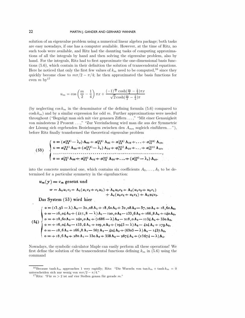
solution of an eigenvalue problem using a numerical linear algebra package; both tasksare easy nowadays, if one has a computer available. However, at the time of Ritz, nosuch tools were available, and Ritz had the daunting tasks of computing approxima-tions of all the integrals by hand and then solving the eigenvalue problem, also byhand. For the integrals, Ritz had to first approximate the one-dimensional basis func-tions (5.6), which contain in their definition the solution of transcendental equations.Here he noticed that only the first few values of km need to be computed,16 since theyquickly become close to mπ/2 − π/4; he then approximated the basis functions foreven m by17
um = cos
(m
2− 1
4
)πx+
(−1)m2 cosh(m2 − 1
4 )πx√2 cosh(m2 − 1
4 )π
(by neglecting cos km in the denominator of the defining formula (5.6) compared tocoshkm) and by a similar expression for odd m. Further approximations were neededthroughout (“Begnugt man sich mit vier genauen Ziffern . . . ,” “Mit einer Genauigkeitvon mindestens 2 Prozent . . . ,” “Zur Vereinfachung wird man die aus der Symmetrieder Losung sich ergebenden Beziehungen zwischen den Amn sogleich einfuhren. . . ”),before Ritz finally transformed the theoretical eigenvalue problem
into the concrete numerical one, which contains six coefficients A0, . . . , A5 to be de-termined for a particular symmetry in the eigenfunction:
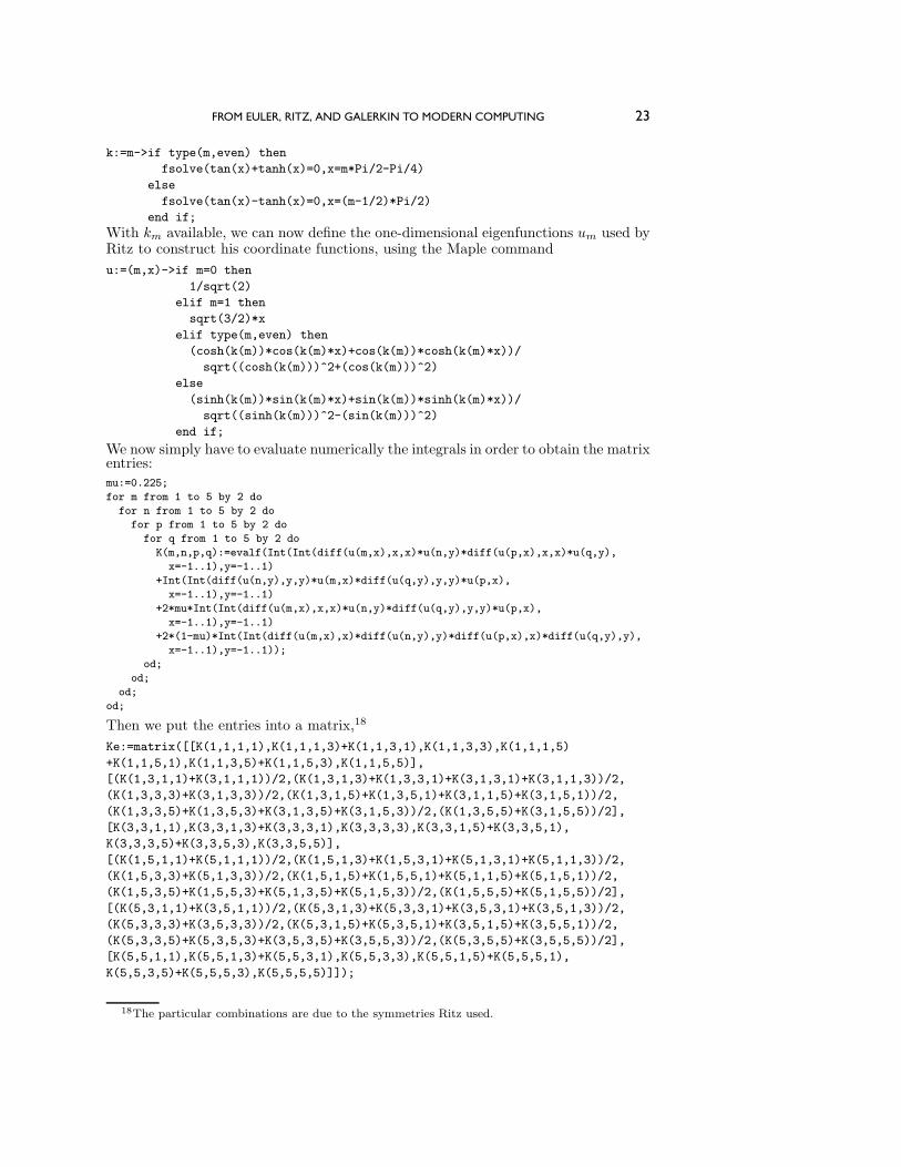
Nowadays, the symbolic calculator Maple can easily perform all these operations! Wefirst define the solution of the transcendental functions defining km in (5.6) using thecommand
16Because tanh km approaches 1 very rapidly; Ritz: “Die Wurzeln von tan km + tanh km = 0unterscheiden sich nur wenig von mπ/2− π/4.”
17Ritz: “Fur m > 2 ist auf vier Stellen genau fur gerade m.”
FROM EULER, RITZ, AND GALERKIN TO MODERN COMPUTING 23
k:=m->if type(m,even) then
fsolve(tan(x)+tanh(x)=0,x=m*Pi/2-Pi/4)
else
fsolve(tan(x)-tanh(x)=0,x=(m-1/2)*Pi/2)
end if;
With km available, we can now define the one-dimensional eigenfunctions um used byRitz to construct his coordinate functions, using the Maple command
u:=(m,x)->if m=0 then
1/sqrt(2)
elif m=1 then
sqrt(3/2)*x
elif type(m,even) then
(cosh(k(m))*cos(k(m)*x)+cos(k(m))*cosh(k(m)*x))/
sqrt((cosh(k(m)))^2+(cos(k(m)))^2)
else
(sinh(k(m))*sin(k(m)*x)+sin(k(m))*sinh(k(m)*x))/
sqrt((sinh(k(m)))^2-(sin(k(m)))^2)
end if;
We now simply have to evaluate numerically the integrals in order to obtain the matrixentries:
mu:=0.225;
for m from 1 to 5 by 2 do
for n from 1 to 5 by 2 do
for p from 1 to 5 by 2 do
for q from 1 to 5 by 2 do
K(m,n,p,q):=evalf(Int(Int(diff(u(m,x),x,x)*u(n,y)*diff(u(p,x),x,x)*u(q,y),
x=-1..1),y=-1..1)
+Int(Int(diff(u(n,y),y,y)*u(m,x)*diff(u(q,y),y,y)*u(p,x),
x=-1..1),y=-1..1)
+2*mu*Int(Int(diff(u(m,x),x,x)*u(n,y)*diff(u(q,y),y,y)*u(p,x),
x=-1..1),y=-1..1)
+2*(1-mu)*Int(Int(diff(u(m,x),x)*diff(u(n,y),y)*diff(u(p,x),x)*diff(u(q,y),y),
x=-1..1),y=-1..1));
od;
od;
od;
od;
Then we put the entries into a matrix,18
Ke:=matrix([[K(1,1,1,1),K(1,1,1,3)+K(1,1,3,1),K(1,1,3,3),K(1,1,1,5)
+K(1,1,5,1),K(1,1,3,5)+K(1,1,5,3),K(1,1,5,5)],
[(K(1,3,1,1)+K(3,1,1,1))/2,(K(1,3,1,3)+K(1,3,3,1)+K(3,1,3,1)+K(3,1,1,3))/2,
(K(1,3,3,3)+K(3,1,3,3))/2,(K(1,3,1,5)+K(1,3,5,1)+K(3,1,1,5)+K(3,1,5,1))/2,
(K(1,3,3,5)+K(1,3,5,3)+K(3,1,3,5)+K(3,1,5,3))/2,(K(1,3,5,5)+K(3,1,5,5))/2],
[K(3,3,1,1),K(3,3,1,3)+K(3,3,3,1),K(3,3,3,3),K(3,3,1,5)+K(3,3,5,1),
K(3,3,3,5)+K(3,3,5,3),K(3,3,5,5)],
[(K(1,5,1,1)+K(5,1,1,1))/2,(K(1,5,1,3)+K(1,5,3,1)+K(5,1,3,1)+K(5,1,1,3))/2,
(K(1,5,3,3)+K(5,1,3,3))/2,(K(1,5,1,5)+K(1,5,5,1)+K(5,1,1,5)+K(5,1,5,1))/2,
(K(1,5,3,5)+K(1,5,5,3)+K(5,1,3,5)+K(5,1,5,3))/2,(K(1,5,5,5)+K(5,1,5,5))/2],
[(K(5,3,1,1)+K(3,5,1,1))/2,(K(5,3,1,3)+K(5,3,3,1)+K(3,5,3,1)+K(3,5,1,3))/2,
(K(5,3,3,3)+K(3,5,3,3))/2,(K(5,3,1,5)+K(5,3,5,1)+K(3,5,1,5)+K(3,5,5,1))/2,
(K(5,3,3,5)+K(5,3,5,3)+K(3,5,3,5)+K(3,5,5,3))/2,(K(5,3,5,5)+K(3,5,5,5))/2],
[K(5,5,1,1),K(5,5,1,3)+K(5,5,3,1),K(5,5,3,3),K(5,5,1,5)+K(5,5,5,1),
K(5,5,3,5)+K(5,5,5,3),K(5,5,5,5)]]);
18The particular combinations are due to the symmetries Ritz used.
24 MARTIN J. GANDER AND GERHARD WANNER
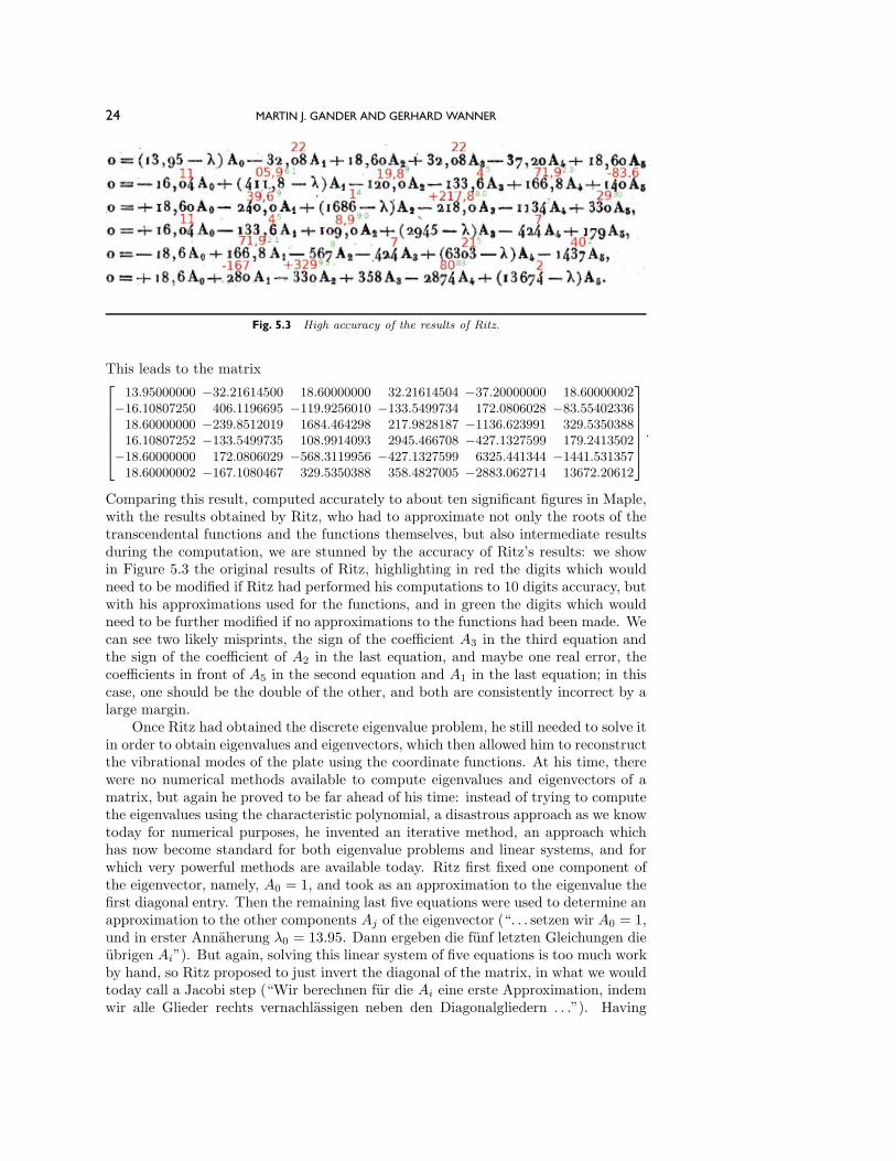
Fig. 5.3 High accuracy of the results of Ritz.
This leads to the matrix⎡⎢⎢⎢⎢⎢⎢⎣
13.95000000 −32.21614500 18.60000000 32.21614504 −37.20000000 18.60000002−16.10807250 406.1196695 −119.9256010 −133.5499734 172.0806028 −83.5540233618.60000000 −239.8512019 1684.464298 217.9828187 −1136.623991 329.535038816.10807252 −133.5499735 108.9914093 2945.466708 −427.1327599 179.2413502
−18.60000000 172.0806029 −568.3119956 −427.1327599 6325.441344 −1441.53135718.60000002 −167.1080467 329.5350388 358.4827005 −2883.062714 13672.20612
⎤⎥⎥⎥⎥⎥⎥⎦.
Comparing this result, computed accurately to about ten significant figures in Maple,with the results obtained by Ritz, who had to approximate not only the roots of thetranscendental functions and the functions themselves, but also intermediate resultsduring the computation, we are stunned by the accuracy of Ritz’s results: we showin Figure 5.3 the original results of Ritz, highlighting in red the digits which wouldneed to be modified if Ritz had performed his computations to 10 digits accuracy, butwith his approximations used for the functions, and in green the digits which wouldneed to be further modified if no approximations to the functions had been made. Wecan see two likely misprints, the sign of the coefficient A3 in the third equation andthe sign of the coefficient of A2 in the last equation, and maybe one real error, thecoefficients in front of A5 in the second equation and A1 in the last equation; in thiscase, one should be the double of the other, and both are consistently incorrect by alarge margin.
Once Ritz had obtained the discrete eigenvalue problem, he still needed to solve itin order to obtain eigenvalues and eigenvectors, which then allowed him to reconstructthe vibrational modes of the plate using the coordinate functions. At his time, therewere no numerical methods available to compute eigenvalues and eigenvectors of amatrix, but again he proved to be far ahead of his time: instead of trying to computethe eigenvalues using the characteristic polynomial, a disastrous approach as we knowtoday for numerical purposes, he invented an iterative method, an approach whichhas now become standard for both eigenvalue problems and linear systems, and forwhich very powerful methods are available today. Ritz first fixed one component ofthe eigenvector, namely, A0 = 1, and took as an approximation to the eigenvalue thefirst diagonal entry. Then the remaining last five equations were used to determine anapproximation to the other components Aj of the eigenvector (“. . . setzen wir A0 = 1,und in erster Annaherung λ0 = 13.95. Dann ergeben die funf letzten Gleichungen dieubrigen Ai”). But again, solving this linear system of five equations is too much workby hand, so Ritz proposed to just invert the diagonal of the matrix, in what we wouldtoday call a Jacobi step (“Wir berechnen fur die Ai eine erste Approximation, indemwir alle Glieder rechts vernachlassigen neben den Diagonalgliedern . . .”). Having
FROM EULER, RITZ, AND GALERKIN TO MODERN COMPUTING 25
this approximation for the eigenvector, one can now compute a correction to theeigenvalue using the first equation, and, according to Ritz, one or two successiveiterations suffice in order to obtain about four digits of accuracy (“Ein oder zweisukzessive Korrektionen genugen meist, um die vierte Stelle bis auf wenige Einheitenfestzustellen”). It is worthwhile to write this algorithm in today’s notation: solvingthe eigenvalue problem
Ka = λa
for a := (a0, a1, . . . , an) and λ is equivalent to solving the nonlinear system of equa-tions
f(λ, a1, . . . , an) := Ka− λa = 0,
where we have fixed, like Ritz, one component of the eigenvector, a0 := 1. Ritz’salgorithm now starts with λ0 = 13.95 and (a01, . . . , a
0n) = 0, and computes for iteration
index k = 0, 1, . . .
fj(λk, ak1 , . . . , a
kj−1, a
k+1j , akj+1, . . . , a
kn) = 0, j = 1, 2, . . . , n,(5.13)
and then solves for a new approximation of the eigenvalue λk+1
f0(λk+1, ak+1
1 , . . . , ak+1n ) = 0.
Note that in each step of the algorithm, only a scalar linear equation needs to besolved. Implementing this method in MATLAB gives the following short program:
K=[13.95 -32.08 18.60 32.08 -37.20 18.60
-16.04 411.8 -120.0 -133.6 166.8 140
18.60 -240.0 1686 -218.0 -1134 330
16.04 -133.6 109.0 2945 -424 179
-18.6 166.8 -567 -424 6303 -1437
18.6 280 -330 358 -2874 13674];
Kr=K(2:end,2:end); % last 5 equations
Kd=diag(Kr); % Jacobi splitting for Ritz’
Ko=Kr-diag(diag(Kr)); % eigenvalue iteration
la=K(1,1) % first eigenvalue and
a=zeros(1,size(K,2)); a(1)=1; % eigenvector approximation
for j=1:6 % Ritz iteration
b=-K(2:end,1); % rhs of the system
bj=b-Ko*a(2:end)’; % rhs for Jacobi step
a(2:6)=bj./(Kd-la) % Jacobi step
la=K(1,1)+K(1,2:end)*a(2:6)’ % new eigenvalue approximation
end
whose output is
26 MARTIN J. GANDER AND GERHARD WANNER
la =
13.9500
a =
1.0000 0.0403 -0.0111 -0.0055 0.0030 -0.0014
la =
12.1388
a =
1.0000 0.0342 -0.0038 -0.0027 0.0002 -0.0017
la =
12.6565
a =
1.0000 0.0387 -0.0061 -0.0036 0.0011 -0.0020
la =
12.3996
a =
1.0000 0.0374 -0.0049 -0.0032 0.0007 -0.0020
la =
12.4972
a =
1.0000 0.0380 -0.0053 -0.0034 0.0009 -0.0020
la =
12.4525
a =
1.0000 0.0378 -0.0051 -0.0033 0.0008 -0.0020
la =
12.4711
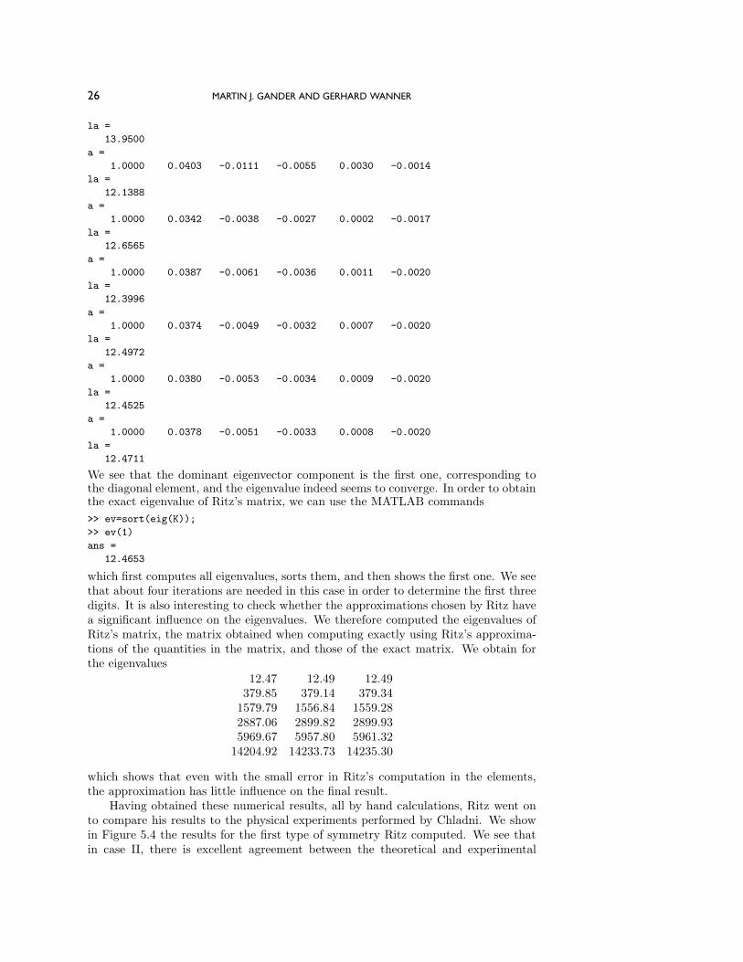
We see that the dominant eigenvector component is the first one, corresponding tothe diagonal element, and the eigenvalue indeed seems to converge. In order to obtainthe exact eigenvalue of Ritz’s matrix, we can use the MATLAB commands
>> ev=sort(eig(K));
>> ev(1)
ans =
12.4653
which first computes all eigenvalues, sorts them, and then shows the first one. We seethat about four iterations are needed in this case in order to determine the first threedigits. It is also interesting to check whether the approximations chosen by Ritz havea significant influence on the eigenvalues. We therefore computed the eigenvalues ofRitz’s matrix, the matrix obtained when computing exactly using Ritz’s approxima-tions of the quantities in the matrix, and those of the exact matrix. We obtain forthe eigenvalues
12.47 12.49 12.49379.85 379.14 379.341579.79 1556.84 1559.282887.06 2899.82 2899.935969.67 5957.80 5961.32
14204.92 14233.73 14235.30
which shows that even with the small error in Ritz’s computation in the elements,the approximation has little influence on the final result.
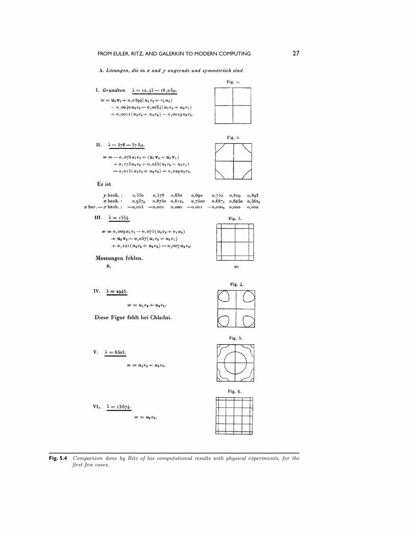
Having obtained these numerical results, all by hand calculations, Ritz went onto compare his results to the physical experiments performed by Chladni. We showin Figure 5.4 the results for the first type of symmetry Ritz computed. We see thatin case II, there is excellent agreement between the theoretical and experimental
FROM EULER, RITZ, AND GALERKIN TO MODERN COMPUTING 27
Fig. 5.4 Comparison done by Ritz of his computational results with physical experiments, for thefirst few cases.
28 MARTIN J. GANDER AND GERHARD WANNER
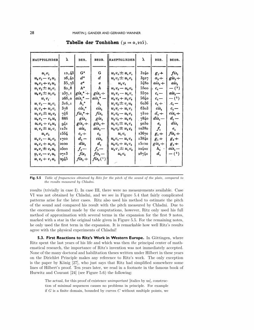
Fig. 5.5 Table of frequencies obtained by Ritz for the pitch of the sound of the plate, compared tothe results measured by Chladni.
results (trivially in case I). In case III, there were no measurements available. CaseVI was not obtained by Chladni, and we see in Figure 5.4 that fairly complicatedpatterns arise for the later cases. Ritz also used his method to estimate the pitchof the sound and compared his result with the pitch measured by Chladni. Due tothe enormous demand made by the computations, however, Ritz only used his fullmethod of approximation with several terms in the expansion for the first 9 notes,marked with a star in the original table given in Figure 5.5. For the remaining notes,he only used the first term in the expansion. It is remarkable how well Ritz’s resultsagree with the physical experiments of Chladni!
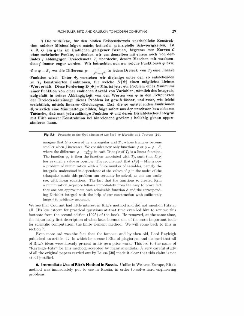
5.3. First Reactions to Ritz’s Work in Western Europe. In Gottingen, whereRitz spent the last years of his life and which was then the principal center of math-ematical research, the importance of Ritz’s invention was not immediately accepted.None of the many doctoral and habilitation theses written under Hilbert in these yearson the Dirichlet Principle makes any reference to Ritz’s work. The only exceptionis the paper by Konig [27], who just says that Ritz had simplified somewhere somelines of Hilbert’s proof. Ten years later, we read in a footnote in the famous book ofHurwitz and Courant [24] (see Figure 5.6) the following:
The actual, for this proof of existence unimportant [italics by us], construc-
tion of minimal sequences causes no problems in principle. For example
if G is a finite domain, bounded by curves C without multiple points, we
FROM EULER, RITZ, AND GALERKIN TO MODERN COMPUTING 29
Fig. 5.6 Footnote in the first edition of the book by Hurwitz and Courant [24].
imagine that G is covered by a triangular grid Tj , whose triangles become
smaller when j increases. We consider now only functions ϕ or φ = ϕ−S,
where the difference ϕ− xx2+y2 in each Triangle of Tj is a linear function.
The function φj is then the function associated with Tj , such that D[φ]
has as small a value as possible. The requirement that D[φ] = Min is now
a problem of minimization with a finite number of variables, namely the
integrals, understood in dependence of the values of ϕ in the nodes of the
triangular mesh; this problem can certainly be solved, as one can easily
see, with linear equations. The fact that the functions so created form
a minimization sequence follows immediately from the easy to prove fact
that one can approximate each admissible function φ and the correspond-
ing Dirichlet integral with the help of our construction with sufficiently
large j to arbitrary accuracy.
We see that Courant had little interest in Ritz’s method and did not mention Ritz atall. His low esteem for practical questions at that time even led him to remove thisfootnote from the second edition (1925) of the book. He removed, at the same time,the historically first description of what later became one of the most important toolsfor scientific computation, the finite element method. We will come back to this insection 7.
Even more sad was the fact that the famous, and by then old, Lord Rayleighpublished an article [42] in which he accused Ritz of plagiarism and claimed that allof Ritz’s ideas were already present in his own prior work. This led to the name of“Rayleigh–Ritz” for this method, accepted by many scientists. A very careful studyof all the original papers carried out by Leissa [30] made it clear that this claim is notat all justified.
6. Immediate Use of Ritz’s Method in Russia. Unlike in Western Europe, Ritz’smethod was immediately put to use in Russia, in order to solve hard engineeringproblems.
30 MARTIN J. GANDER AND GERHARD WANNER
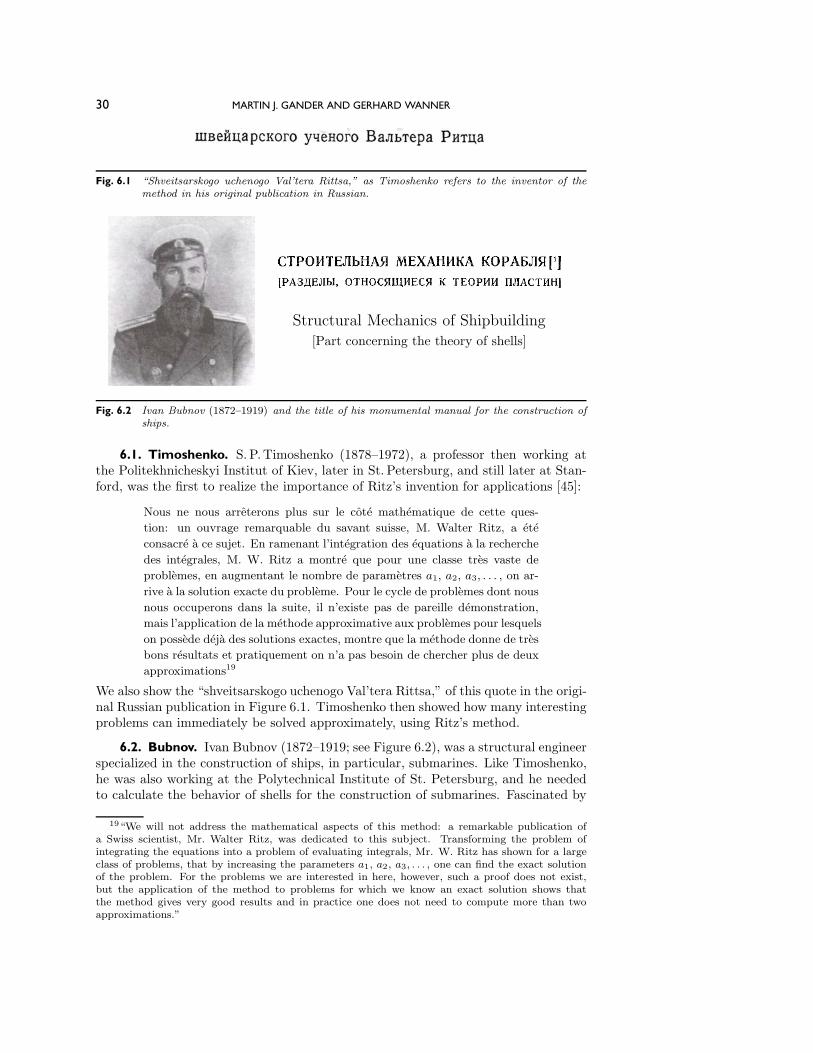
Fig. 6.1 “Shveitsarskogo uchenogo Val’tera Rittsa,” as Timoshenko refers to the inventor of themethod in his original publication in Russian.
Structural Mechanics of Shipbuilding[Part concerning the theory of shells]
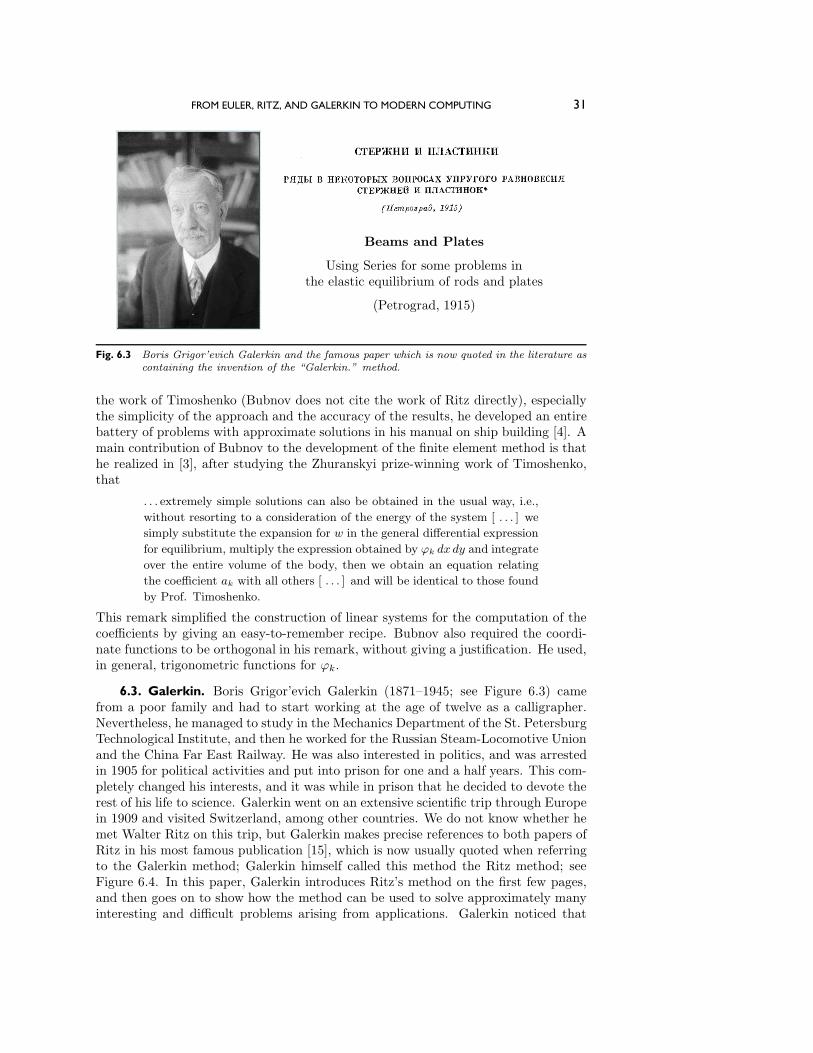
Fig. 6.2 Ivan Bubnov (1872–1919) and the title of his monumental manual for the construction ofships.
6.1. Timoshenko. S. P.Timoshenko (1878–1972), a professor then working atthe Politekhnicheskyi Institut of Kiev, later in St. Petersburg, and still later at Stan-ford, was the first to realize the importance of Ritz’s invention for applications [45]:
Nous ne nous arreterons plus sur le cote mathematique de cette ques-
tion: un ouvrage remarquable du savant suisse, M. Walter Ritz, a ete
consacre a ce sujet. En ramenant l’integration des equations a la recherche
des integrales, M. W. Ritz a montre que pour une classe tres vaste de
problemes, en augmentant le nombre de parametres a1, a2, a3, . . . , on ar-
rive a la solution exacte du probleme. Pour le cycle de problemes dont nous
nous occuperons dans la suite, il n’existe pas de pareille demonstration,
mais l’application de la methode approximative aux problemes pour lesquels
on possede deja des solutions exactes, montre que la methode donne de tres
bons resultats et pratiquement on n’a pas besoin de chercher plus de deux
approximations19
We also show the “shveitsarskogo uchenogo Val’tera Rittsa,” of this quote in the origi-nal Russian publication in Figure 6.1. Timoshenko then showed how many interestingproblems can immediately be solved approximately, using Ritz’s method.
6.2. Bubnov. Ivan Bubnov (1872–1919; see Figure 6.2), was a structural engineerspecialized in the construction of ships, in particular, submarines. Like Timoshenko,he was also working at the Polytechnical Institute of St. Petersburg, and he neededto calculate the behavior of shells for the construction of submarines. Fascinated by
19“We will not address the mathematical aspects of this method: a remarkable publication ofa Swiss scientist, Mr. Walter Ritz, was dedicated to this subject. Transforming the problem ofintegrating the equations into a problem of evaluating integrals, Mr. W. Ritz has shown for a largeclass of problems, that by increasing the parameters a1, a2, a3, . . . , one can find the exact solutionof the problem. For the problems we are interested in here, however, such a proof does not exist,but the application of the method to problems for which we know an exact solution shows thatthe method gives very good results and in practice one does not need to compute more than twoapproximations.”
FROM EULER, RITZ, AND GALERKIN TO MODERN COMPUTING 31
Beams and Plates
Using Series for some problems inthe elastic equilibrium of rods and plates
(Petrograd, 1915)
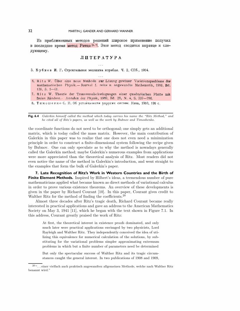
Fig. 6.3 Boris Grigor’evich Galerkin and the famous paper which is now quoted in the literature ascontaining the invention of the “Galerkin.” method.
the work of Timoshenko (Bubnov does not cite the work of Ritz directly), especiallythe simplicity of the approach and the accuracy of the results, he developed an entirebattery of problems with approximate solutions in his manual on ship building [4]. Amain contribution of Bubnov to the development of the finite element method is thathe realized in [3], after studying the Zhuranskyi prize-winning work of Timoshenko,that
. . . extremely simple solutions can also be obtained in the usual way, i.e.,
without resorting to a consideration of the energy of the system [ . . . ] we
simply substitute the expansion for w in the general differential expression
for equilibrium, multiply the expression obtained by ϕk dx dy and integrate
over the entire volume of the body, then we obtain an equation relating
the coefficient ak with all others [ . . . ] and will be identical to those found
by Prof. Timoshenko.
This remark simplified the construction of linear systems for the computation of thecoefficients by giving an easy-to-remember recipe. Bubnov also required the coordi-nate functions to be orthogonal in his remark, without giving a justification. He used,in general, trigonometric functions for ϕk.
6.3. Galerkin. Boris Grigor’evich Galerkin (1871–1945; see Figure 6.3) camefrom a poor family and had to start working at the age of twelve as a calligrapher.Nevertheless, he managed to study in the Mechanics Department of the St. PetersburgTechnological Institute, and then he worked for the Russian Steam-Locomotive Unionand the China Far East Railway. He was also interested in politics, and was arrestedin 1905 for political activities and put into prison for one and a half years. This com-pletely changed his interests, and it was while in prison that he decided to devote therest of his life to science. Galerkin went on an extensive scientific trip through Europein 1909 and visited Switzerland, among other countries. We do not know whether hemet Walter Ritz on this trip, but Galerkin makes precise references to both papers ofRitz in his most famous publication [15], which is now usually quoted when referringto the Galerkin method; Galerkin himself called this method the Ritz method; seeFigure 6.4. In this paper, Galerkin introduces Ritz’s method on the first few pages,and then goes on to show how the method can be used to solve approximately manyinteresting and difficult problems arising from applications. Galerkin noticed that
32 MARTIN J. GANDER AND GERHARD WANNER
· · ·
· · ·
Fig. 6.4 Galerkin himself called the method which today carries his name the “Ritz Method,” andhe cited all of Ritz’s papers, as well as the work by Bubnov and Timoshenko.
the coordinate functions do not need to be orthogonal; one simply gets an additionalmatrix, which is today called the mass matrix. However, the main contribution ofGalerkin in this paper was to realize that one does not even need a minimizationprinciple in order to construct a finite-dimensional system following the recipe givenby Bubnov. One can only speculate as to why the method is nowadays generallycalled the Galerkin method; maybe Galerkin’s numerous examples from applicationswere more appreciated than the theoretical analysis of Ritz. Most readers did noteven notice the name of the method in Galerkin’s introduction, and went straight tothe examples that form the bulk of Galerkin’s paper.
7. Late Recognition of Ritz’s Work in Western Countries and the Birth ofFinite Element Methods. Inspired by Hilbert’s ideas, a tremendous number of puremathematicians applied what became known as direct methods of variational calculusin order to prove various existence theorems. An overview of these developments isgiven in the paper by Richard Courant [10]. In this paper, Courant gives credit toWalther Ritz for the method of finding the coefficients.20
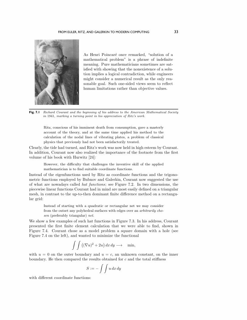
Almost three decades after Ritz’s tragic death, Richard Courant became reallyinterested in practical applications and gave an address to the American MathematicsSociety on May 3, 1941 [11], which he began with the text shown in Figure 7.1. Inthis address, Courant greatly praised the work of Ritz:
At first, the theoretical interest in existence proofs dominated, and only
much later were practical applications envisaged by two physicists, Lord
Rayleigh and Walther Ritz. They independently conceived the idea of uti-
lizing this equivalence for numerical calculation of the solutions, by sub-
stituting for the variational problems simpler approximating extremum
problems in which but a finite number of parameters need be determined
But only the spectacular success of Walther Ritz and its tragic circum-
stances caught the general interest. In two publications of 1908 and 1909,
20“. . . einer vielfach auch praktisch angewandten allgemeinen Methode, welche nach Walther Ritzbenannt wird.”
FROM EULER, RITZ, AND GALERKIN TO MODERN COMPUTING 33
As Henri Poincare once remarked, “solution of amathematical problem” is a phrase of indefinitemeaning. Pure mathematicians sometimes are sat-isfied with showing that the nonexistence of a solu-tion implies a logical contradiction, while engineersmight consider a numerical result as the only rea-sonable goal. Such one-sided views seem to reflecthuman limitations rather than objective values.
Fig. 7.1 Richard Courant and the beginning of his address to the American Mathematical Societyin 1941, marking a turning point in his appreciation of Ritz’s work.
Ritz, conscious of his imminent death from consumption, gave a masterly
account of the theory, and at the same time applied his method to the
calculation of the nodal lines of vibrating plates, a problem of classical
physics that previously had not been satisfactorily treated.
Clearly, the tide had turned, and Ritz’s work was now held in high esteem by Courant.In addition, Courant now also realized the importance of the footnote from the firstvolume of his book with Hurwitz [24]:
However, the difficulty that challenges the inventive skill of the applied
mathematician is to find suitable coordinate functions.
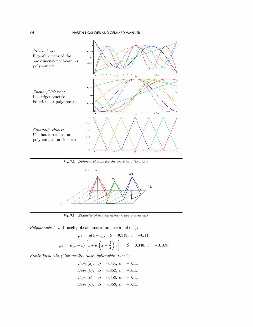
Instead of the eigenfunctions used by Ritz as coordinate functions and the trigono-metric functions employed by Bubnov and Galerkin, Courant now suggested the useof what are nowadays called hat functions ; see Figure 7.2. In two dimensions, thepiecewise linear functions Courant had in mind are most easily defined on a triangularmesh, in contrast to the up-to-then dominant finite difference method on a rectangu-lar grid:
Instead of starting with a quadratic or rectangular net we may consider
from the outset any polyhedral surfaces with edges over an arbitrarily cho-
sen (preferably triangular) net.
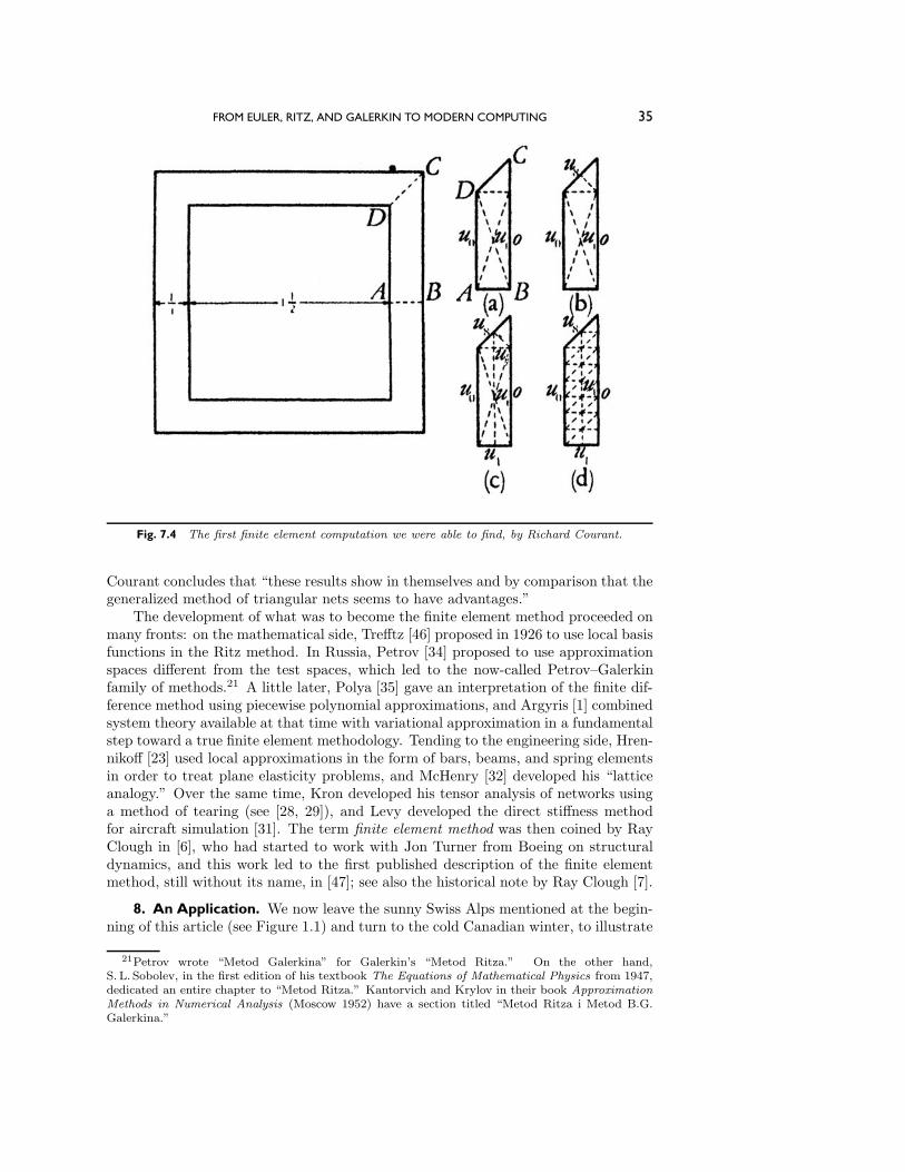
We show a few examples of such hat functions in Figure 7.3. In his address, Courantpresented the first finite element calculation that we were able to find, shown inFigure 7.4. Courant chose as a model problem a square domain with a hole (seeFigure 7.4 on the left), and wanted to minimize the functional∫ ∫ (
(∇u)2 + 2u)dx dy −→ min,
with u = 0 on the outer boundary and u = c, an unknown constant, on the innerboundary. He then compared the results obtained for c and the total stiffness
S := −∫ ∫
u dx dy
with different coordinate functions:
34 MARTIN J. GANDER AND GERHARD WANNER
Ritz’s choice:Eigenfunctions of theone-dimensional beam, orpolynomials
Bubnov/Galerkin:Use trigonometricfunctions or polynomials
Courant’s choice:Use hat functions, orpolynomials on elements
Fig. 7.2 Different choices for the coordinate functions.
x
y
u ϕi
ϕj
ϕk
Fig. 7.3 Examples of hat functions in two dimensions.
Polynomials (“with negligible amount of numerical labor”):
ϕ1 := a(1− x), S = 0.339, c = −0.11,
ϕ2 := a(1− x)
[1 + α
(x− 3
4
)y
], S = 0.340, c = −0.109.
Finite Elements (“the results, easily obtainable, were”):
Case (a): S = 0.344, c = −0.11.
Case (b): S = 0.352, c = −0.11.
Case (c): S = 0.353, c = −0.11.
Case (d): S = 0.353, c = −0.11.
FROM EULER, RITZ, AND GALERKIN TO MODERN COMPUTING 35
Fig. 7.4 The first finite element computation we were able to find, by Richard Courant.
Courant concludes that “these results show in themselves and by comparison that thegeneralized method of triangular nets seems to have advantages.”
The development of what was to become the finite element method proceeded onmany fronts: on the mathematical side, Trefftz [46] proposed in 1926 to use local basisfunctions in the Ritz method. In Russia, Petrov [34] proposed to use approximationspaces different from the test spaces, which led to the now-called Petrov–Galerkinfamily of methods.21 A little later, Polya [35] gave an interpretation of the finite dif-ference method using piecewise polynomial approximations, and Argyris [1] combinedsystem theory available at that time with variational approximation in a fundamentalstep toward a true finite element methodology. Tending to the engineering side, Hren-nikoff [23] used local approximations in the form of bars, beams, and spring elementsin order to treat plane elasticity problems, and McHenry [32] developed his “latticeanalogy.” Over the same time, Kron developed his tensor analysis of networks usinga method of tearing (see [28, 29]), and Levy developed the direct stiffness methodfor aircraft simulation [31]. The term finite element method was then coined by RayClough in [6], who had started to work with Jon Turner from Boeing on structuraldynamics, and this work led to the first published description of the finite elementmethod, still without its name, in [47]; see also the historical note by Ray Clough [7].
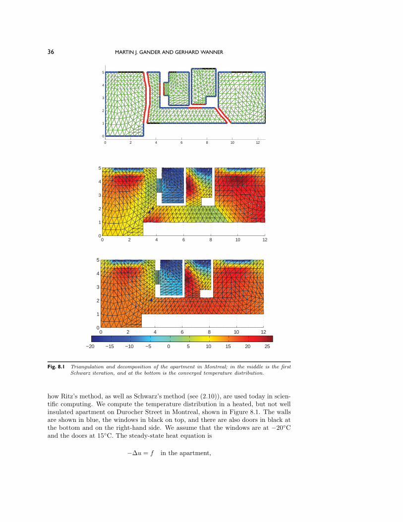
8. An Application. We now leave the sunny Swiss Alps mentioned at the begin-ning of this article (see Figure 1.1) and turn to the cold Canadian winter, to illustrate
21Petrov wrote “Metod Galerkina” for Galerkin’s “Metod Ritza.” On the other hand,S. L. Sobolev, in the first edition of his textbook The Equations of Mathematical Physics from 1947,dedicated an entire chapter to “Metod Ritza.” Kantorvich and Krylov in their book ApproximationMethods in Numerical Analysis (Moscow 1952) have a section titled “Metod Ritza i Metod B.G.Galerkina.”
36 MARTIN J. GANDER AND GERHARD WANNER
0 2 4 6 8 10 12
0
1
2
3
4
5
0 2 4 6 8 10 120
1
2
3
4
5
−20 −15 −10 −5 0 5 10 15 20 25
0 2 4 6 8 10 120
1
2
3
4
5
Fig. 8.1 Triangulation and decomposition of the apartment in Montreal; in the middle is the firstSchwarz iteration, and at the bottom is the converged temperature distribution.
how Ritz’s method, as well as Schwarz’s method (see (2.10)), are used today in scien-tific computing. We compute the temperature distribution in a heated, but not wellinsulated apartment on Durocher Street in Montreal, shown in Figure 8.1. The wallsare shown in blue, the windows in black on top, and there are also doors in black atthe bottom and on the right-hand side. We assume that the windows are at −20◦Cand the doors at 15◦C. The steady-state heat equation is
−Δu = f in the apartment,
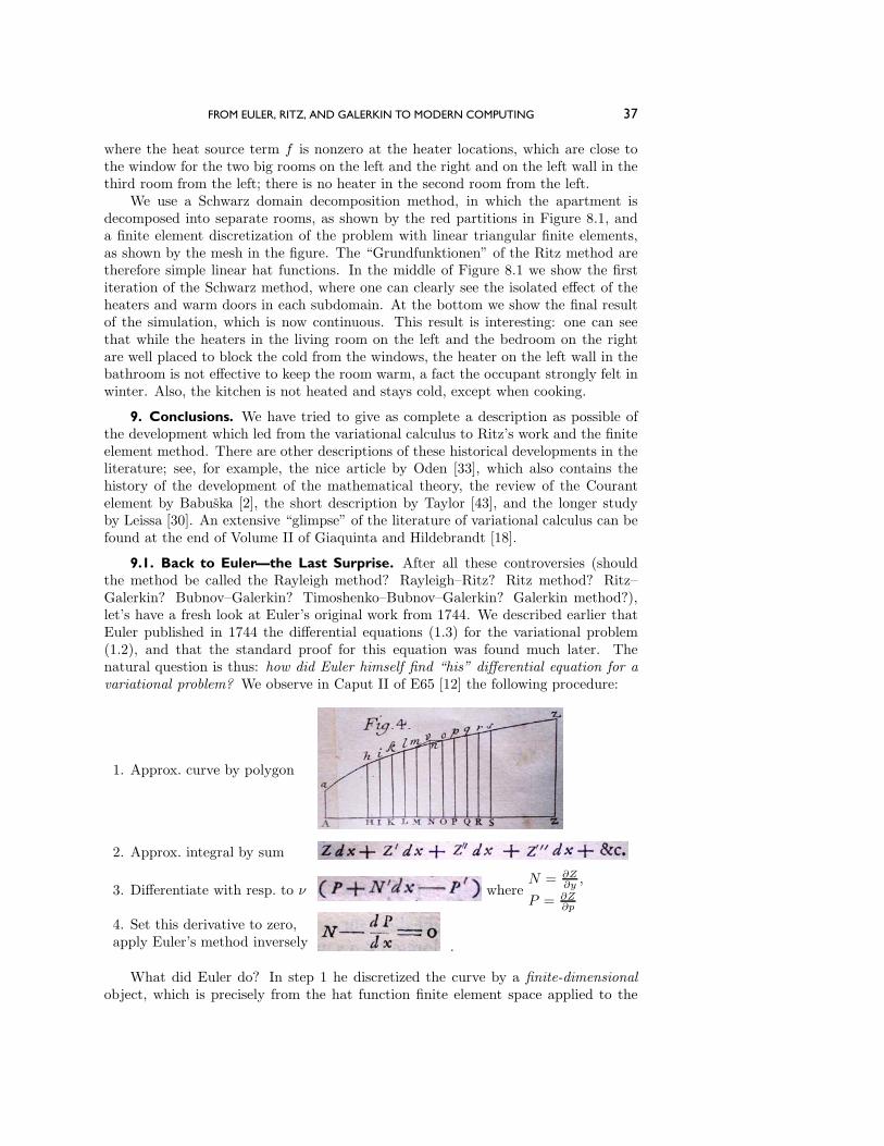
FROM EULER, RITZ, AND GALERKIN TO MODERN COMPUTING 37
where the heat source term f is nonzero at the heater locations, which are close tothe window for the two big rooms on the left and the right and on the left wall in thethird room from the left; there is no heater in the second room from the left.
We use a Schwarz domain decomposition method, in which the apartment isdecomposed into separate rooms, as shown by the red partitions in Figure 8.1, anda finite element discretization of the problem with linear triangular finite elements,as shown by the mesh in the figure. The “Grundfunktionen” of the Ritz method aretherefore simple linear hat functions. In the middle of Figure 8.1 we show the firstiteration of the Schwarz method, where one can clearly see the isolated effect of theheaters and warm doors in each subdomain. At the bottom we show the final resultof the simulation, which is now continuous. This result is interesting: one can seethat while the heaters in the living room on the left and the bedroom on the rightare well placed to block the cold from the windows, the heater on the left wall in thebathroom is not effective to keep the room warm, a fact the occupant strongly felt inwinter. Also, the kitchen is not heated and stays cold, except when cooking.
9. Conclusions. We have tried to give as complete a description as possible ofthe development which led from the variational calculus to Ritz’s work and the finiteelement method. There are other descriptions of these historical developments in theliterature; see, for example, the nice article by Oden [33], which also contains thehistory of the development of the mathematical theory, the review of the Courantelement by Babuska [2], the short description by Taylor [43], and the longer studyby Leissa [30]. An extensive “glimpse” of the literature of variational calculus can befound at the end of Volume II of Giaquinta and Hildebrandt [18].
9.1. Back to Euler—the Last Surprise. After all these controversies (shouldthe method be called the Rayleigh method? Rayleigh–Ritz? Ritz method? Ritz–Galerkin? Bubnov–Galerkin? Timoshenko–Bubnov–Galerkin? Galerkin method?),let’s have a fresh look at Euler’s original work from 1744. We described earlier thatEuler published in 1744 the differential equations (1.3) for the variational problem(1.2), and that the standard proof for this equation was found much later. Thenatural question is thus: how did Euler himself find “his” differential equation for avariational problem? We observe in Caput II of E65 [12] the following procedure:
1. Approx. curve by polygon
2. Approx. integral by sum
3. Differentiate with resp. to ν whereN = ∂Z
∂y ,
P = ∂Z∂p
4. Set this derivative to zero,apply Euler’s method inversely .
What did Euler do? In step 1 he discretized the curve by a finite-dimensionalobject, which is precisely from the hat function finite element space applied to the
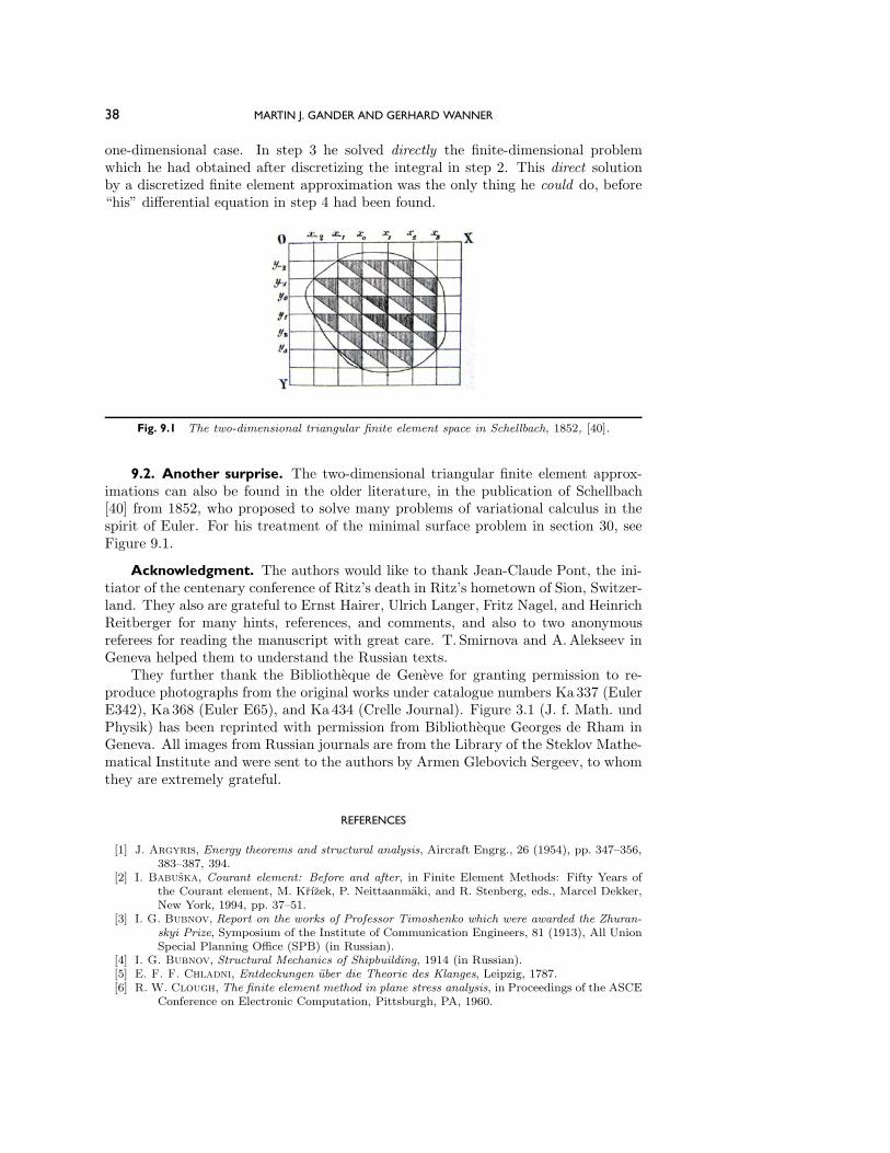
38 MARTIN J. GANDER AND GERHARD WANNER
one-dimensional case. In step 3 he solved directly the finite-dimensional problemwhich he had obtained after discretizing the integral in step 2. This direct solutionby a discretized finite element approximation was the only thing he could do, before“his” differential equation in step 4 had been found.
Fig. 9.1 The two-dimensional triangular finite element space in Schellbach, 1852, [40].
9.2. Another surprise. The two-dimensional triangular finite element approx-imations can also be found in the older literature, in the publication of Schellbach[40] from 1852, who proposed to solve many problems of variational calculus in thespirit of Euler. For his treatment of the minimal surface problem in section 30, seeFigure 9.1.
Acknowledgment. The authors would like to thank Jean-Claude Pont, the ini-tiator of the centenary conference of Ritz’s death in Ritz’s hometown of Sion, Switzer-land. They also are grateful to Ernst Hairer, Ulrich Langer, Fritz Nagel, and HeinrichReitberger for many hints, references, and comments, and also to two anonymousreferees for reading the manuscript with great care. T. Smirnova and A.Alekseev inGeneva helped them to understand the Russian texts.
They further thank the Bibliotheque de Geneve for granting permission to re-produce photographs from the original works under catalogue numbers Ka 337 (EulerE342), Ka 368 (Euler E65), and Ka 434 (Crelle Journal). Figure 3.1 (J. f. Math. undPhysik) has been reprinted with permission from Bibliotheque Georges de Rham inGeneva. All images from Russian journals are from the Library of the Steklov Mathe-matical Institute and were sent to the authors by Armen Glebovich Sergeev, to whomthey are extremely grateful.
REFERENCES
[1] J. Argyris, Energy theorems and structural analysis, Aircraft Engrg., 26 (1954), pp. 347–356,383–387, 394.
[2] I. Babuska, Courant element: Before and after, in Finite Element Methods: Fifty Years ofthe Courant element, M. Krızek, P. Neittaanmaki, and R. Stenberg, eds., Marcel Dekker,New York, 1994, pp. 37–51.
[3] I. G. Bubnov, Report on the works of Professor Timoshenko which were awarded the Zhuran-skyi Prize, Symposium of the Institute of Communication Engineers, 81 (1913), All UnionSpecial Planning Office (SPB) (in Russian).
[4] I. G. Bubnov, Structural Mechanics of Shipbuilding, 1914 (in Russian).[5] E. F. F. Chladni, Entdeckungen uber die Theorie des Klanges, Leipzig, 1787.[6] R. W. Clough, The finite element method in plane stress analysis, in Proceedings of the ASCE
Conference on Electronic Computation, Pittsburgh, PA, 1960.
FROM EULER, RITZ, AND GALERKIN TO MODERN COMPUTING 39
[7] R. W. Clough, Thoughts about the origin of the finite element method, Comput. & Structures,79 (2001), pp. 2029–2030.
[8] R. Courant, Uber die Anwendung des Dirichletschen Prinzipes auf die Probleme der konfor-men Abbildung, Math. Ann., 71 (1912), pp. 145–183.
[9] R. Courant, Uber die Existenztheoreme der Potential- und Funktionentheorie, J. ReineAngew. Math., 144 (1914), pp. 190–211.
[10] R. Courant, Uber direkte Methoden in der Variationsrechnung und uber verwandte Fragen,Math. Ann., 97 (1927), pp. 711–736.
[11] R. Courant, Variational methods for the solution of problems of equilibrium and vibrations,Bull. Amer. Math. Soc., 49 (1943), pp. 1–61.
[12] L. Euler, Methodus inveniendi lineas curvas maximi minimive proprietate gaudentes sivesolutio problematis isoperimetrici latissimo sensu accepti, Lausannae & Genevae, 1744.Enestr. 65, Opera Omnia, Ser. I, Vol. 24.
[13] L. Euler, Institutionum calculi integralis, Petropolis, 1768. Enestr. 342, Opera Omnia, Ser.I,vol. 11.
[14] L. Euler, Methodus Nova et Facilis Calculum Variationum Tractandi, Noci commentarii acad.scient. Petropolitanae, 16 (1772), pp. 35–70. Enestr. 420, Opera Omnia, Ser. I, Vol. 25,pp. 208–235.
[15] B. G. Galerkin, Rods and plates. Series occurring in various questions concerning the elasticequilibrium of rods and plates, Engineers Bulletin (Vestnik Inzhenerov), 19 (1915), pp. 897–908 (in Russian).
[16] C. F. Gauss, Allgemeine Lehrsatze in Beziehung auf die im verkehrten Verhaltnisse desQuadrates der Entfernung wirkenden Anziehungs- und Abstossungs-Krafte, MagnetischerVerein, 1839. Werke Vol. 5, pp. 195–242.
[17] M. Giaquinta and S. Hildebrandt, Calculus of Variations. I, Springer, Berlin, 1996.[18] M. Giaquinta and S. Hildebrandt, Calculus of Variations. II, Springer, Berlin, 1996.[19] M. H. Gutknecht, Numerical experiments on solving Theodorsen’s integral equation for con-
formal maps with the fast Fourier transform and various nonlinear iterative methods,SIAM J. Sci. Statist. Comput., 4 (1983), pp. 1–30.
[20] P. Henrici, Applied and Computational Complex Analysis, Vol. 3, John Wiley, New York,1986.
[21] D. Hilbert, Uber das Dirichletsche Prinzip, Jahresbericht der Deutschen Mathematiker-Vereinigung, 8 (1900), pp. 184–188. Reprinted in J. Reine Angew. Math., 129 (1905),pp. 63–67.
[22] D. Hilbert, Uber das Dirichletsche Prinzip, Math. Ann., 59 (1904), pp. 161–186.[23] A. Hrennikoff, Solution of problems of elasticity by the frame-work method, ASME J. Appl.
Mech., 8 (1941), pp. 615–715.[24] A. Hurwitz and R. Courant, Vorlesungen uber die allgemeine Funktionentheorie und ellip-
tische Funktionen, Julius Springer, Berlin, 1922.[25] G. Kirchhoff, Uber das Gleichgewicht und die Bewegung einer elastischen Scheibe, J. Reine
Angew. Math., 44 (1850), pp. 51–92.[26] R. Konig, Beitrag zur Theorie der Klangfiguren von Wheatstone, Annalen der Physik und
Chemie/Poggendorfs Annalen, 122 (1864), pp. 238–245.[27] R. Konig, Konforme Abbildung der Oberflache einer raumlichen Ecke, Math. Ann., 71 (1912),
pp. 184–205.[28] G. Kron, Tensor Analysis of Networks, John Wiley, New York, 1939.[29] G. Kron, A set of principles to interconnect the solutions of physical systems, J. Appl. Phys.,
24 (1953), pp. 965–980.[30] A. W. Leissa, The historical bases of the Rayleigh and Ritz methods, J. Sound Vibration, 287
(2005), pp. 961–978.[31] S. Levy, Structural analysis and influence coefficients for delta wings, J. Aeronautical Sci., 20
(1953), pp. XXX–XXX.[32] D. McHenry, A lattice analogy for the solution of plane stress problems, J. Inst. Civ. Eng., 21
(1943), pp. 59–82.[33] J. T. Oden, Historical comments on finite elements, in A History of Scientific Computing
(Princeton, NJ, 1987), ACM, New York, 1990, pp. 152–166.[34] G. I. Petrov, Application of Galerkin’s method to the problem of stability of flow of a viscous
fluid, J. Appl. Math. Mech., 4 (1940), pp. 3–12 (in Russian).[35] G. Polya, Sur une interpretation de la methode des differences finis qui peut fournir des bornes
superieures ou inferieures, C. R. Acad. Sci. Paris, 235 (1952), pp. 995–997.[36] B. Riemann, Grundlagen fur eine allgemeine Theorie der Functionen einer veranderlichen
complexen Grosse, Inauguraldissertation Gottingen, 1851 (Gesammelte Werke, pp. 3–43).
40 MARTIN J. GANDER AND GERHARD WANNER
[37] B. Riemann, Bestimmung einer Function einer veranderlichen complexen Grosse durch Grenz-und Unstetigkeitsbedingungen, J. Reine Angew. Math., 54 (1857), pp. 111–114 (GesammelteWerke, pp. 96–100).
[38] W. Ritz, Uber eine neue Methode zur Losung gewisser Variationsprobleme der mathema-tischen Physik, J. Reine Angew. Math., 135 (1908), pp. 1–61.
[39] W. Ritz, Theorie der Transversalschwingungen einer quadratischen Platte mit freien Randern,Ann. Phys., 18 (1909), pp. 737–807.
[40] K. Schellbach, Probleme der Variationsrechnung, J. Reine Angew. Math., 41 (1852), pp. 293–363.
[41] J. W. Strutt (Lord Rayleigh), The Theory of Sound, Vol. I, Macmillan, London, 1894. Newedition, Dover, New York, 1945.
[42] J. W. Strutt (Lord Rayleigh), On the calculation of Chladni’s figures for a square plate,Philosophical Magazine Sixth Series, 22 (1911), pp. 225–229.
[43] R. L. Taylor, Ritz & Galerkin: The road to the finite element method, Bull. Internat. Assoc.Comput. Mech., 12 (2002), pp. 2–5.
[44] W. Thomson (later Lord Kelvin), Sur une equation aux differences partielles qui se presentedans plusieurs questions de Physique mathematique, J. Math. Pures Appl., 12 (1847),pp. 493–496.
[45] S. P. Timoshenko, Sur la stabilite des systemes elastiques, Annales des Ponts et Chaussees,9 (1913), pp. 496–566. Traduit du russe par M. Jean Karpinski et Victor Heroufosse;originally published in Russian in Isvestija Kievskogo Politechnitscheskogo Instituta, Kiev,1910.
[46] E. Trefftz, Ein Gegenstuck zum Ritzschen Verfahren, 2. Int. Kongress fur TechnischeMechanik, Zurich, 1926, pp. 131–137.
[47] N. J. Turner, R. W. Clough, H. C. Martin, and L. J. Topp, Stiffness and deflectionanalysis of complex structures, J. Aeronautical Sci., 23 (1956), pp. 805–823.
[48] W. Voigt, Bemerkung zu dem Problem der transversalen Schwingungen rechteckiger Platten,Gottinger Nachrichten 1893, pp. 225–230.
[49] K. T. W. Weierstrass, Uber das sogenannte Dirichletsche Prinzip, Werke, 2 (1895), pp. 49–54. Read in the Academy Berlin, 14 July 1870.
[50] C. Wheatstone, On the figures obtained by strewing sand on vibrating surfaces, commonlycalled acoustic figures, Philos. Trans. Roy. Soc., 123 (1833), pp. 593–634.