1 Chapter 7 Cooperative Strategy PART III CREATING COMPETITIVE ADVANTAGE.

From Competitive to Cooperative ResourceManagement for Cyber-Physical Systems
Mikael Lindberg
Department of Automatic Control

PhD ThesisISRN LUTFD2/TFRT--1102--SEISBN 978-91-7623-018-3 (print)ISBN 978-91-7623-019-0 (web)ISSN 0280–5316
Department of Automatic ControlLund UniversityBox 118SE-221 00 LUNDSweden
c© 2014 by Mikael Lindberg. All rights reserved.Printed in Sweden by MediaTryck.Lund 2014

To Mirjam, Mattis and Rebecka


Abstract
This thesis presents models and methods for feedback-based resource managementfor cyber-physical systems. Common for the scenarios considered are severe re-source constraints, uncertain and time-varying conditions and the goal of enablingflexibility in systems design rather than restricting it.
A brief survey on reservation-based scheduling, an important enabling technol-ogy for this thesis, is provided and shows how modern day resource reservationtechniques are derived from their real-time system and telecommunications theoryroots.
Techniques for modeling components of cyber-physical systems, including bothcomputational and physical resources, are presented. The cyclic component model,specifically designed to model common resource demanding components in smartphones, is introduced together with techniques for model parameter estimation.
The topic of competitive resource management, where the different parts of thesystem compete for resources, is discussed using a smart phone platform as motivat-ing example. The cyclic component model is used to form a rate-based performancemetric that results in a convex optimization problem. A specialized optimization al-gorithm for solving this problem efficiently online and with limited precision hard-ware is introduced and evaluated through simulations.
A feedback control scheme for distributing resources in cases where compo-nents collaborate, i.e., where the performance metric is dependent on more thanone component, is detailed and examined in a scenario where the available resourceis limited by the thermal dynamics of the CPU. The scheme is evaluated throughsimulation of a conversational video pipeline. The thermal model is validated on amobile robot, where it is used as part of an adaptive resource manager.
The problem of energy conservative distribution of content to a population ofco-located mobile clients is used to motivate the chapter on cooperative resourcemanagement, i.e., scenarios where the participants have individual but similar goalsand can benefit from sharing their partial results so that all collaborators save cost.The model for content trading is presented in synchronous and asynchronous for-mulations and performance is evaluated through both simulations and experimentalresults using a prototype implementation in an emulated environment.
5


Acknowledgements
It is safe to say that this thesis would not have existed if not for some of the amazingpeople I am privileged to be surrounded by. Combining my PhD studies with thebusy life of fatherhood, and with my penchant for maintaining far too many hob-bies and interests, has been a challenging and instructive journey, the completion ofwhich I feel I must share some credits for.
Breaking off my career and returning to school for a PhD was not a decisionI made lightly, and I feel very fortunate for the opportunity to do so. My thanksto Anders Robertsson for tricking me into this. I vividly remember the Thursdayevening you called me and suggested I apply for the position, and I can assure allreaders that there will be repercussions somewhere down the line.
Throughout my time at the department I have been able to rely on Eva Westinfor support, friendship, advice and candy. She is an amazing person whom I hopewill get all the recognition she deserves for what she does, both professionally andsocially. Eva, my door is always open for you.
I wish to express my gratitude to my supervisor, Professor Karl-Erik Årzén, whohas listened to my sometimes wild ideas and who has been a pillar of support duringstressful moments of my studies. You have always had time for me when I askedfor it and provided good directions, for research as well as for pubs.
To my co-supervisor, Johan Eker, I wish to extend my thanks for the discussionswe had and for the much needed coaching during periods of doubt and uncertainty.Your levelheaded yet diligent approach to research has taught me many things Ihope to incorporate into my own methods as I continue this path. And yes, I willprobably buy that piano.
While I have been one of the older PhD students at the department, it has beencomforting to always be put in place by the research engineers. Anders Blomdell,Leif Andersson and Rolf Braun, you have my thanks for your help, your dedication,and for constantly reminding me just how little I still know.
During my PhD years I have had many colleagues, some of which has becomegood friends. I would specifically like to mention Toivo Henningsson, my mentorat the department, whose enthusiasm and insights have inspired my work. I wouldalso like to thank Anders Widd and Martin Hast for the conversations we had and
7

Karl Berntorp for paving the way during the thesis writing period. Coffee is on mefrom now on.
Though perhaps not consciously aware of their contributions, I would like tomention my children, Mattis and Rebecka, as some of the more important influ-ences for my work. There is no finer way to study dynamic constrained resourcemanagement than observing our hallway in the morning as we are trying to geteverybody off to school and work.
Last but not least, I would like to thank my wife Mirjam for her unwaveringsupport during these years. Despite everything, I have never heard you regret oncethat we took this decision, even though my own resolve has sometimes wavered.There is no person to whom I owe more, nor any person I would rather have by myside for the next challenge.
Mikael
This research has partially been funded by the VINNOVA/Ericsson project"Feedback Based Resource Management and Code Generation for Real-time Sys-tem" , the EU ICT project CHAT (ICT-224428), the EU NoE ArtistDesign, theLinneaus Center LCCC, the ELLIIT strategic research center, and the Ack’a VRproject 2011-3635 "Feedback-based resource management for embedded multicoreplatforms".
8
Contents
1. Introduction 131.1 Background and motivation . . . . . . . . . . . . . . . . . . . . 131.2 Contributions . . . . . . . . . . . . . . . . . . . . . . . . . . . 161.3 Outline of the thesis . . . . . . . . . . . . . . . . . . . . . . . . 17
2. Problem formulation 182.1 Example 1 — Smartphones . . . . . . . . . . . . . . . . . . . . 182.2 Example 2 — Mobile robotics . . . . . . . . . . . . . . . . . . . 212.3 Example 3 – Mobile cloud computing . . . . . . . . . . . . . . . 232.4 Problem features . . . . . . . . . . . . . . . . . . . . . . . . . . 242.5 Problem structures . . . . . . . . . . . . . . . . . . . . . . . . . 242.6 Overall goals . . . . . . . . . . . . . . . . . . . . . . . . . . . . 25
3. Reservation based scheduling 273.1 Important concepts . . . . . . . . . . . . . . . . . . . . . . . . . 273.2 Reservation Based Scheduling . . . . . . . . . . . . . . . . . . . 293.3 Feedback allocation control . . . . . . . . . . . . . . . . . . . . 363.4 Allocation . . . . . . . . . . . . . . . . . . . . . . . . . . . . . 383.5 Reservation frameworks . . . . . . . . . . . . . . . . . . . . . . 393.6 The Xen hypervisor . . . . . . . . . . . . . . . . . . . . . . . . 433.7 Xenomai . . . . . . . . . . . . . . . . . . . . . . . . . . . . . . 433.8 Linux Control Groups . . . . . . . . . . . . . . . . . . . . . . . 443.9 Estimating software model parameters . . . . . . . . . . . . . . 44
4. Power and energy management 464.1 Energy and resources . . . . . . . . . . . . . . . . . . . . . . . 464.2 Spatial resource management, "E-logistics" . . . . . . . . . . . . 49
5. Modeling and Estimation 525.1 Smartphone model . . . . . . . . . . . . . . . . . . . . . . . . . 525.2 Allocation and utility . . . . . . . . . . . . . . . . . . . . . . . 535.3 Components with rate-based utility . . . . . . . . . . . . . . . . 555.4 Multi-resource dependencies . . . . . . . . . . . . . . . . . . . 595.5 CPU thermal dynamics . . . . . . . . . . . . . . . . . . . . . . 60
9

Contents
5.6 Parameter estimation . . . . . . . . . . . . . . . . . . . . . . . 605.7 Extension into mixed domain models . . . . . . . . . . . . . . . 63
6. Competitive resource management 656.1 Allocation under resource constraints . . . . . . . . . . . . . . . 656.2 Incremental optimization . . . . . . . . . . . . . . . . . . . . . 676.3 Experimental results . . . . . . . . . . . . . . . . . . . . . . . . 716.4 Implementation . . . . . . . . . . . . . . . . . . . . . . . . . . 736.5 Resource management architecture . . . . . . . . . . . . . . . . 756.6 Measuring time and resource consumption . . . . . . . . . . . . 776.7 Example runs . . . . . . . . . . . . . . . . . . . . . . . . . . . 796.8 Conclusions . . . . . . . . . . . . . . . . . . . . . . . . . . . . 79
7. Collaborative resource management 837.1 Allocation vs feedback . . . . . . . . . . . . . . . . . . . . . . 837.2 State related performance metrics . . . . . . . . . . . . . . . . . 847.3 Hardware resources . . . . . . . . . . . . . . . . . . . . . . . . 867.4 Case study — Encoding Pipeline . . . . . . . . . . . . . . . . . 877.5 Simulation results . . . . . . . . . . . . . . . . . . . . . . . . . 917.6 Thermal control through resource management . . . . . . . . . . 967.7 Control design . . . . . . . . . . . . . . . . . . . . . . . . . . . 1017.8 Implementation . . . . . . . . . . . . . . . . . . . . . . . . . . 1047.9 Experimental results . . . . . . . . . . . . . . . . . . . . . . . . 1057.10 Conclusions . . . . . . . . . . . . . . . . . . . . . . . . . . . . 109
8. Cooperative resource management 1118.1 Increasing focus on the local . . . . . . . . . . . . . . . . . . . 1118.2 Incentivizing cooperation . . . . . . . . . . . . . . . . . . . . . 1128.3 System model . . . . . . . . . . . . . . . . . . . . . . . . . . . 1148.4 The dynamics of fair exchanges . . . . . . . . . . . . . . . . . . 1158.5 Baseline algorithm . . . . . . . . . . . . . . . . . . . . . . . . . 1198.6 Heuristic solver . . . . . . . . . . . . . . . . . . . . . . . . . . 1218.7 Set sizes and problem decomposition . . . . . . . . . . . . . . . 1288.8 Random initial state . . . . . . . . . . . . . . . . . . . . . . . . 1338.9 Continuous operation . . . . . . . . . . . . . . . . . . . . . . . 1348.10 Asynchronous formulation . . . . . . . . . . . . . . . . . . . . 1388.11 Software design . . . . . . . . . . . . . . . . . . . . . . . . . . 1398.12 Experimental results . . . . . . . . . . . . . . . . . . . . . . . . 1428.13 Conclusions . . . . . . . . . . . . . . . . . . . . . . . . . . . . 148
9. Conclusions and future work 1499.1 Conclusions . . . . . . . . . . . . . . . . . . . . . . . . . . . . 1499.2 Future work . . . . . . . . . . . . . . . . . . . . . . . . . . . . 150
Bibliography 154A. Listings 164
10

Contents
A.1 MIPC . . . . . . . . . . . . . . . . . . . . . . . . . . . . . . . . 164
11

1Introduction
1.1 Background and motivation
Resource management considerations are increasingly shaping the development ofnew technology, be it embedded computers or large scale infrastructure systems,and the limits of realizable functionality is often defined by factors such as energy oravailable network bandwidth. The current global focus on designing energy efficientsystems and ecologically sustainable technological growth is likely to emphasizethese issues even further in the foreseeable future.
With that in mind, the central theme of this thesis is chosen to be resource man-agement for computer systems. While resource management for embedded systemshas for a long time been modeled as real-time scheduling problems, such methodsare primarily used in monolithic systems with well known structure. This thesischooses instead to focus on the highly dynamic and uncertain cases introduced bythe increasingly advanced types of embedded systems developed today.
Systems controlled by software are inherently flexible and reconfigurable. En-abling system designers to use this flexibility while retaining control over systemperformance is an important goal of this work. Feedback, estimation and onlineoptimization take the place of current methods based on prior knowledge, and themodels employed are tailored towards a holistic point of view, where the inclusionof both physical and computational resource dynamics is necessary to describe sys-tem performance.
It is the intention of this work to propose new ways to view resource manage-ment for computer- and cyber-physical systems, so that their potential can be fur-ther explored. The resource management techniques provided by scheduling theorytherefore form a part of the schemes discussed rather than being the focal point ofthem.
The methods presented draw upon several disciplines to provide a frameworkfor resource management, including
• control theory,
• system identification,
13

Chapter 1. Introduction
• convex optimization,
• reservation based scheduling, and
• peer-to-peer technology.
The target systems are embedded or cyber-physical systems that are such that re-source constraints and uncertainty would make worst case methods infeasible.
The thesis is based on the following publications:
Lindberg, M. (2007). A Survey of Reservation-Based Scheduling. Technical Re-port ISRN LUTFD2/TFRT--7618--SE. Department of Automatic Control, LundUniversity, Sweden.
This technical report is a survey on the state of the art concerning reservation-based scheduling. The survey covers the origins of the field as it appears both inreal-time computing and telecommunication and how the two fields have merged inpresent day.
M. Lindberg was the author of the report and collected the information it wasbased on.
Lindberg, M. (2009). “Constrained online resource control using convex program-ming based allocation”. In: Proceedings of the 4th International Workshop onFeedback Control Implementation and Design in Computing Systems and Net-works (FeBID 2009).
This paper presents a model for resource reservations for smart phones, basedon convex optimization. Included is also an algorithm aimed at limited precisionhardware to solve the optimization problem in an efficient manner.
M. Lindberg formulated the model, designed and implemented the optimizationalgorithm, and conducted experiments in order to examine the performance of thealgorithm. M. Lindberg was also the author of the paper.
Lindberg, M. (2010). “Convex programming-based resource management for un-certain execution platforms”. In: Proceedings of First International Workshopon Adaptive Resource Management. Stockholm, Sweden.
The contributions of this paper consists of the implementation of a resourcemanager based on the allocation algorithm presented in the previous papers and theresults of experiments where the performance of the system is studied under timevarying conditions. The paper also presents a model for cyclic software componentsthat can be used to describe many types of resource demanding applications.
14
1.1 Background and motivation
M. Lindberg developed the component model, implemented the resource man-ager and performed the experiments in the paper. He is also the author of the publi-cation.
Lindberg, M. (2010). “A convex optimization-based approach to control of uncer-tain execution platforms”. In: Proceedings of the 49th IEEE Conference on De-cision and Control. Atlanta, Georgia, USA.
This paper is a rewritten version of the previous paper aimed at am automaticcontrol audience. The models are reworked to better fit within the control domain.
M. Lindberg is the author of this paper and did the textual revision as well asthe adaptation of the resource models.
Lindberg, M. and K.-E. Årzén (2010). “Feedback control of cyber-physical systemswith multi resource dependencies and model uncertainties”. In: Proc. 31st IEEEReal-Time Systems Symposium. San Diego, CA.
This paper presents a model for collaborative resource management for inter-connected components as well as a model for thermal control of an embeddedCPU through constrained resource allocation. The paper presents a case study ofa conversational video pipeline, with continuous thermal dynamics for the CPU.A scheme for feedback control-based optimization of performance metrics is dis-cussed together with simulation results.
M. Lindberg is the originator of the approach as well as the designer of thefeedback control mechanism. M. Lindberg also developed the software used forsimulations and is the author of this paper. K.E. Årzén contributed the problemintroduction and background.
Romero Segovia, V., M. Kralmark, M. Lindberg, and K.-E. Årzén (2011). “Proces-sor thermal control using adaptive bandwidth resource management”. In: Pro-ceedings of IFAC World Congress, Milan, Italy. Milano, Italy.
In this paper, thermal CPU control based on dynamic resource allocation isdemonstrated on a mobile robot. The contributions consists of experiments to vali-date the thermal model used in the previous paper on the robot as well as test caseswith synthetic tasks running on the robot under time varying conditions.
M. Lindberg contributed the thermal control approach and the basic idea for theexperiment and authored the part of the paper concerning the thermal control. V.Romero-Segovia designed the resource reservation part of the experimental set-upand wrote the sections in the paper that covers this. M. Kralmark performed theexperiments on the robot. K.E. Årzén provided valuable input and reviewed thepublication.
15

Chapter 1. Introduction
Lindberg, M. (2013). “Feedback-based cooperative content distribution for mobilenetworks”. In: The 16th ACM International Conference on Modeling, Analysisand Simulation of Wireless and Mobile Systems. Barcelona, Spain.
The paper introduces a scheme for energy conservation for content distributionin mobile networks. The contributions consists of a definition of the cooperativemechanism through which co-located mobile devices can exchange data so that allparties save energy and a feedback-based algorithm for optimizing the trades inreal-time. The approach is evaluated through simulations.
M. Lindberg formulated the cooperative mechanism, designed the heuristicfeedback mechanism and developed the simulation software used for the experi-ments. M. Lindberg is also the author of the paper.
Lindberg, M. (2014). “Analysis of a feedback-based energy conserving contentdistribution mechanism for mobile networks”. In: Proceedings of IFAC WorldCongress 2014.
This paper expands on the cooperative scheme with time varying device pop-ulations and studies the throughput of the system under changing conditions. Theresulting findings are discussed together with a design example.
M. Lindberg developed the software used to study the expanded cooperativedistribution problem. performed the experiments and created the design example.M. Lindberg is also the author of the paper.
Lindberg, M. (2014). “A prototype implementation of an energy-conservative co-operative content distribution system”. In: The 17th ACM International Confer-ence on Modeling, Analysis and Simulation of Wireless and Mobile Systems. Insubmission.
A prototype implementation of the cooperative distribution scheme is presentedtogether with a modified asynchronous formulation of the underlying system model.The implementation is validated through experiments carried out in an emulatedenvironment using laboratory PCs.
M. Lindberg contributed the asynchronous model and developed the softwareused for the experiments. M. Lindberg carried out the experiments and is the authorof the paper.
1.2 Contributions
This thesis contains the following contributions
• A model for resource allocation for rate-based software components is pro-posed. The model is suitable for many types of applications that typically
16

1.3 Outline of the thesis
require the most resources in cyber-physical systems, such as media players,controllers and games.
• An algorithm for solving convex allocation problems suitable for embeddedplatforms has been developed. The algorithm is designed to be easily imple-mented in fix-point arithmetics and with a varying problem structure.
• A control scheme for software components with multi resource dependen-cies is proposed. The scheme is intended to facilitate the integration of thephysical and the computational aspects of a system.
• Experimental results from using CPU bandwidth reservation for thermal con-trol are detailed. Experiments were conducted on a mobile robot using aLinux-based operating system and standard Intel-based hardware.
• An energy and spectrum conserving cooperative content distribution mecha-nism for wireless mobile devices using barter-like data trade is proposed. Themechanism uses a feedback-based arbitration algorithm in order to be viablein highly dynamic cases.
• A prototype implementation of the aforementioned mechanism is presentedtogether with experimental results.
1.3 Outline of the thesis
This thesis is organized into chapters as follows. In Chapter 2, the formal definitionof the problem is given. Chapter 3 presents relevant and related research, partic-ularly covering the enabling technology of reservation based scheduling. Chapter4 presents related results on the topic of power- and energy management. Modelsand estimation techniques suitable for cyber-physical systems with uncertain pa-rameters are introduced in Chapter 5. Chapter 6 discusses resource management insystems where components compete for resources. The collaborative perspective,where components contribute to a common performance metric, is then presentedin Chapter 7. Chapter 8 discusses techniques for cooperative resource management,where system components tries to maximize individual performance through coop-erating. Chapter 9 then concludes with discussion and future research.
17

2Problem formulation
This chapter introduces the problems treated in the thesis. The domain of smart-phones serves as a basis for deriving the formal definition. An example from thecontrol domain is added to provide an example of a resource management prob-lem where components contribute to a common performance metric, and in orderto show that the resource management problem is not unique to multimedia appli-cations. Finally, the smartphone example is expanded into the mobile cloud for-mulation, with multiple independent units, to exemplify a case where units withindividual performance metrics can all benefit from sharing resources.
In the case of smartphones, special attention is given to the point of view of plat-form providers, who would like to increase system robustness without posing overlyprohibitive requirements on applications. In this context, a platform is a hardwareand software design that supplies base functionality and resources. Complete prod-ucts are then constructed by adding components built with a development kit whichis distributed together with the platform. The Google Android platform is a recentexample [Android, 2014].
For the mobile cloud scenario, the phone platform provider serves a more pe-ripheral role as an enabler rather than the main stakeholder. Here it is rather assumedthat the primary parties are phone users, who would like to minimize data trafficfees and maximize battery usage, and service providers that want to reduce networkcongestion.
2.1 Example 1 — Smartphones
The first motivating example comes from the domain of smartphones or tablet de-vices. These consumer products are fully customizable through downloadable ap-plications - "apps" - and are often used for processing-intensive tasks, such as mediaplayback, video recording or games. The exact resource needs for such applicationsis hard to predict as the software behavior in these domains is highly data and usercommand dependent. Since video playback is one of the more demanding tasks,this will be used as an illustrative example.
18

2.1 Example 1 — Smartphones
0 5 10 15 20 25 30 35 40time (s)
8
9
10
11
12
13
14
15
16
CPU
Uti
lizati
on in p
erc
ent
Utilization for 320 x 180 movie
0 5 10 15 20 25 30 35 40time (s)
35
40
45
50
55
60
CPU
Uti
lizati
on in p
erc
ent
Utilization for 1280 x 720 movie
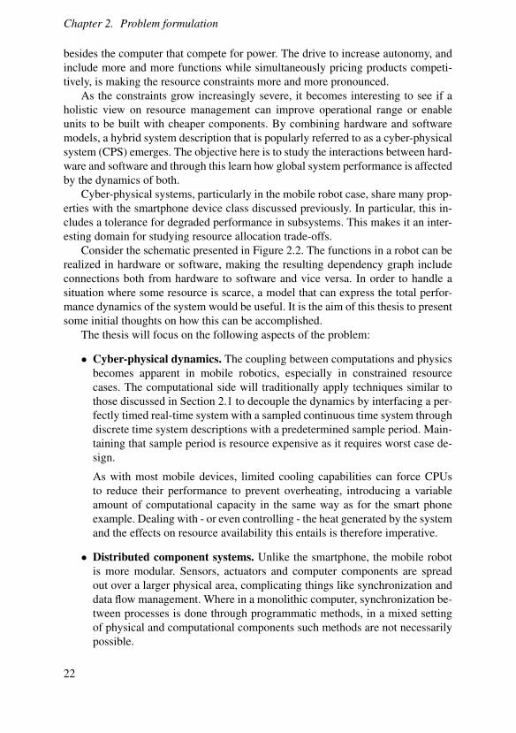
Figure 2.1 Resource requirements for decoding two versions of a H.264 movie onan Intel Core 2 Duo-based MacBook. The left plot represents a movie encoded inlow resolution (320 by 180 pixels) while the right represents one encoded in HDTV-resolution (1280 by 720 pixels). The experiment was run three times with varyingresults, as illustrated by the the three curves in each plot. The utilization measurerepresents the percentage of time the decoding process had exclusive access to theCPU measured with a sliding 1 second time window.
Figure 2.1 exemplifies the CPU utilization for decoding two versions of the samevideo stream with perfect playback, i.e., no frame skipping or playback jitter. Notehow the resource demands are significantly larger for the high resolution stream andhow the levels change over time. There is also a visible trend, with a slight increasein resource demand around 15 seconds and a dip at around 28 seconds. This is evi-dent for both streams and is caused by the encoding standard, which uses differentlevels of compression depending on the level of motion in the source video. Theexperiment was run three times for each stream with different results each time, thisdespite the fact that decoding a specific movie stream is a deterministic sequenceof operations. One major reason for this is that modern hardware relies heavily onprediction and heuristics to minimize effects of memory latency and pipeline bub-bles. Should these strategies fail, the system takes a performance hit. As the systemdoing the decoding in the example is executing a large number of background tasksin addition to the decoder, system state will vary from run to run.
The problem stated in traditional real-time terms would be to check the schedu-
19
Chapter 2. Problem formulation
lability of a set of periodic tasks τ0, ...,τN with the corresponding periods T0, ...,TNand worst case execution times C0, ...,CN . Assume for simplicity that each task hasa relative deadline equal to its period. If the scheduling policy used is Earliest Dead-line First (EDF) and the system is a single core machine, the task set is schedulableif
N
∑i=0
Ci
Ti≤Ub (2.1)
where Ub is the utilization bound, which depends on parameters such as the costof context switches and is normally close to 1. For a media player task, the periodwould be equal to the frame rate at which the movie is encoded, which is easilyaccessible from the stream meta data.
If the test passes, deadlines will be met and the system performs as intended.If the test fails, the system is overloaded and tasks will miss their deadlines. Tra-ditionally, a system should not admit tasks that will cause overload, but given theuncertainties mentioned above, it is not clear if enough information would be avail-able to make such decisions. Specifically,
• the set of active tasks will change over time as the user enables differentapplications,
• the resource requirements of a task can vary greatly depending on input, and
• the properties of 3rd party software might not be available during systemdesign.
A system designer could choose to restrict the use cases supported by the device inorder to counteract some of these points, but this could render the product unattrac-tive to consumers. It is also probable that a user would rather have access to afunction running with degraded performance than being denied this functionalitycompletely. Therefore, the all-or-nothing property of hard real-time formulations isnot suitable for this problem domain.
This thesis chooses to focus on the following aspects of the problem:
• Uncertainty in hardware and software. The reliance on prior information intraditional real-time systems is increasingly a bottleneck in designing feature-rich embedded systems. Rather, the approach taken here will be to try tomodel the resource consumption of a system and estimate model parametersonline.
This has the effect of reducing the work needed by both hardware designersand software developers, thereby reducing time to market for both productand 3rd party add-ons.
• Allocation under overload conditions. For portable devices it is desirable touse low power components (CPUs, batteries, radio transmitters etc) and as a
20

2.2 Example 2 — Mobile robotics
Sensors
TrajectoryPlanning
ServoControl
Higher LevelSupervisoryFunctions
Servos
On boardComputer
cputime
readings
targets refs
controls
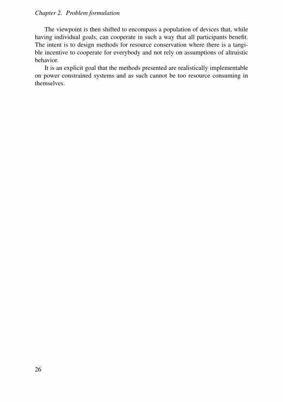
Figure 2.2 A schematic over a simple mobile robot system. The square blocks rep-resent hardware functions that require power, the round-corner shapes are softwarefunctions that require cpu-time to run. The complex dependency situation makes itnon-trivial to determine how to prioritize in a situation with insufficient resources torun the system at nominal performance.
result, efficient systems will often run near or in overload conditions in orderto save power and unit cost.
The thesis will strive to provide resource management strategies that effec-tively manage systems under both nominal and overload conditions.
• Non-restrictive assumptions on software components. One way to sim-plify the work of the system designer would be to shift some of the burdento the 3rd party developers, e.g., requiring them to supply worst case execu-tion time estimates and other detailed resource demand information. As suchfigures require technical expertise with the target platform, this could impedethe supply of attractive 3rd party software.
The application framework should put clear but lenient requirements on de-velopers in order to make the platform simple and attractive to develop for.
2.2 Example 2 — Mobile robotics
Mobile robotics is another field where resource management is key to performance.Not only are computational resources scarce, there are usually many subsystems
21
Chapter 2. Problem formulation
besides the computer that compete for power. The drive to increase autonomy, andinclude more and more functions while simultaneously pricing products competi-tively, is making the resource constraints more and more pronounced.
As the constraints grow increasingly severe, it becomes interesting to see if aholistic view on resource management can improve operational range or enableunits to be built with cheaper components. By combining hardware and softwaremodels, a hybrid system description that is popularly referred to as a cyber-physicalsystem (CPS) emerges. The objective here is to study the interactions between hard-ware and software and through this learn how global system performance is affectedby the dynamics of both.
Cyber-physical systems, particularly in the mobile robot case, share many prop-erties with the smartphone device class discussed previously. In particular, this in-cludes a tolerance for degraded performance in subsystems. This makes it an inter-esting domain for studying resource allocation trade-offs.
Consider the schematic presented in Figure 2.2. The functions in a robot can berealized in hardware or software, making the resulting dependency graph includeconnections both from hardware to software and vice versa. In order to handle asituation where some resource is scarce, a model that can express the total perfor-mance dynamics of the system would be useful. It is the aim of this thesis to presentsome initial thoughts on how this can be accomplished.
The thesis will focus on the following aspects of the problem:
• Cyber-physical dynamics. The coupling between computations and physicsbecomes apparent in mobile robotics, especially in constrained resourcecases. The computational side will traditionally apply techniques similar tothose discussed in Section 2.1 to decouple the dynamics by interfacing a per-fectly timed real-time system with a sampled continuous time system throughdiscrete time system descriptions with a predetermined sample period. Main-taining that sample period is resource expensive as it requires worst case de-sign.
As with most mobile devices, limited cooling capabilities can force CPUsto reduce their performance to prevent overheating, introducing a variableamount of computational capacity in the same way as for the smart phoneexample. Dealing with - or even controlling - the heat generated by the systemand the effects on resource availability this entails is therefore imperative.
• Distributed component systems. Unlike the smartphone, the mobile robotis more modular. Sensors, actuators and computer components are spreadout over a larger physical area, complicating things like synchronization anddata flow management. Where in a monolithic computer, synchronization be-tween processes is done through programmatic methods, in a mixed settingof physical and computational components such methods are not necessarilypossible.
22

2.3 Example 3 – Mobile cloud computing
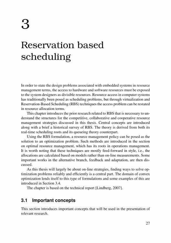
Figure 2.3 The use of cloud computing services, such as remote data storage ormedia streaming, by mobile devices is very natural and in some cases even necessaryin order to deal with limited built in storage and sandboxed applications. What hasyet to happen is the inclusion of the mobile devices as part of the cloud in the formof service providers.
2.3 Example 3 – Mobile cloud computing
The intrinsic limitations of mobile devices in terms of storage or computationalcapacity have made these devices heavily dependent on cloud computing services,such as remote storage or media streaming. With the rapid growth of both devicesand services, it is perhaps not surprising that licensed spectrum is already scarce[FCC, 2010].
In order to reduce network load, it is tempting to implement peer-to-peer or peer-assisted mechanisms popular in fixed networks with stationary computers, such asBitTorrent, but the mobile case presents additional challenges before these tech-nologies can be deployed. The limited energy available to a mobile device makesit inherently unattractive to help distribute data unless guarantees can be given thatsuch investments will pay off.
By creating cooperative mechanisms where mobile devices can share the task offetching data over expensive remote links, without risk of losing energy on the trans-action, the mobile part of the network can be turned into willing service providers.
This thesis discusses how the coupling of resource constraints can lead to suchschemes, where clients cooperate to solve problems and save resources while simul-taneously reducing load on the Wide Area Network (WAN). The specific situationstudied is cooperative file distribution to a population of co-located devices, underassumptions of high mobility and that nobody is willing to act altruistically.
Specifically, the thesis focuses on the following elements of the problem:
• Cooperative sharing of resources Finding ways to create win-win coop-erative scenarios is important for systems of independent units, as altruisticbehavior cannot be expected.
• Dynamic populations As in the case of the individual smart phones, where
23

Chapter 2. Problem formulation
the active software components will vary over time, the population of mobiledevices interested in cooperating will vary over time and space. As such it isimportant that the mechanism uses feedback and estimation to make decisionsand not rely on offline calculated solutions.
2.4 Problem features
A number of structural similarities present themselves in the above examples.
Limited resourcesSystem performance is clearly limited by the availability of resources. Reducingsize while adding functionality has been the trend in consumer electronics for along time, so though components become smaller and more efficient, resource con-straints continue to be an important factor in product design.
Uncertainty and estimationDemand and supply of resources are expected to change over time, either sponta-neously or as a function of how they are used. An example of the former is whencomponents activate or switch modes, where the latter can be a result of the CPUheating up or a battery being drained. It is important to note that not only are systemparameters expected to change over time, but the structure of the system (e.g., whatcomponents are active) is subject to continuous change as well.
Feedback and optimizationRather than relying on pre-calculated solutions, the thesis uses optimization- andfeedback-based techniques to continuously maximize the system utility, given thecurrent system state and resource availability.
Taking decisions on a budgetIn order to make continuous resource allocation decisions viable, the results needto be computed in a timely and resource-light fashion. Many powerful forms ofoptimization are therefore infeasible for this problem domain, due to heavy compu-tational requirements and/or computational complexity that is difficult to predict.
2.5 Problem structures
In this thesis, the problems of resource management will be divided into three cate-gories.
24

2.6 Overall goals
CompetitiveIn a competitive scenario, the components of the system have their own privateperformance metrics, which are functions of the component’s resource allocation.In general, it is up to an outside party to determine the value of each componentin relation to the others, something that is traditionally done in software systemsthrough priority assignment by an outside party, often a system designer or user.
The thesis will generally consider under-provisioned cases, i.e., where there isinsufficient resources to saturate the needs of all components. As the competitivecase concerns systems with unrelated components, one problem is how a systemdesigner can describe the desired compromise and how component designers canexpress the resource needs of their components in a way that is simple and yetrobust to platform changes.
CollaborativeIn collaborative systems, components have no individual performance metrics, butcontribute to one or more system wide metrics. These metrics typically concernthings like synchronized operation, end-to-end latency over a number of compo-nents, and buffer length control.
In over-provisioned cases, these types of problems are often formulated as syn-chronization and mutual exclusion problems, but as locking is problematic in re-source management situations, the thesis offers a different view that can be appliedto general CPS systems where functionality is implemented across both hardwareand software.
CooperativeCooperative systems consist of components with individual performance metrics,but where they can benefit from exchanging data and services. The central themehere is not to allocate resources, but rather to allocate the spending of it so that thereturn on investment is as high as possible. This thesis will analyze an example ofsuch a scheme where mobile clients cooperate around fetching data from a remoteservice and share it locally, thereby reducing both licensed spectrum and energyusage.
2.6 Overall goals
The objective of this work is to investigate how resource management can be donein situations where uncertainty in both demand and supply makes static methodsinfeasible. An effort is made to consider systems where components have depen-dencies, as this topic is less studied. While initially the work was focused on CPUresources inside a computer, the robot example makes it evident that if the avail-ability of the CPU resource depends on the dynamics of other resources, a modelencompassing both domains is desired.
25
Chapter 2. Problem formulation
The viewpoint is then shifted to encompass a population of devices that, whilehaving individual goals, can cooperate in such a way that all participants benefit.The intent is to design methods for resource conservation where there is a tangi-ble incentive to cooperate for everybody and not rely on assumptions of altruisticbehavior.
It is an explicit goal that the methods presented are realistically implementableon power constrained systems and as such cannot be too resource consuming inthemselves.
26
3Reservation basedscheduling
In order to state the design problems associated with embedded systems in resourcemanagement terms, the access to hardware and software resources must be exposedto the system designers as divisible resources. Resource access in computer systemshas traditionally been posed as scheduling problems, but through virtualization andReservation-Based Scheduling (RBS) techniques the access problem can be restatedin resource allocation terms.
This chapter introduces the prior research related to RBS that is necessary to un-derstand the structures for the competitive, collaborative and cooperative resourcemanagement strategies discussed in this thesis. Central concepts are introducedalong with a brief a historical survey of RBS. The theory is derived from both itsreal-time scheduling roots and its queueing theory counterpart.
Using the RBS formulation, a resource management policy can be posed as thesolution to an optimization problem. Such methods are introduced in the sectionon optimal resource management, which has its roots in operations management.It is worth noting that these techniques are mostly feed-forward in style, i.e., theallocations are calculated based on models rather than on-line measurements. Someimportant works in the alternative branch, feedback and adaptation, are then dis-cussed.
As this thesis will largely be about on-line strategies, finding ways to solve op-timization problems reliably and efficiently is a central part. The domain of convexoptimization lends itself to this type of formulations and some examples of this areintroduced in Section 3.4.
The chapter is based on the technical report [Lindberg, 2007].
3.1 Important concepts
This section introduces important concepts that will be used in the presentation ofrelevant research.
27

Chapter 3. Reservation based scheduling
Temporal IsolationA highly desirable property of the RBS approach is that a task that has reserved aspecific amount of a resource should have access to this regardless of what othertasks are running on the system. This is called temporal isolation and makes verygood sense for both continuous media and control type applications used as exam-ples so far. Memory protection ensures that applications will behave functionallycorrect even in the presence of other, potentially malfunctioning, software. Tempo-ral isolation provides a similar guarantee for temporal correctness.
Components and compositionIn order to handle the complexity of large systems, the ability to gather parts intocomponent structures that are closed under composition is vital. Threads with pri-orities, the building blocks of traditional operating systems, do not compose [Lee,2006]. By using hierarchical RBS techniques, it is possible to enforce temporal iso-lation and thereby create groups of threads with essentially the same outside prop-erties as the atomic thread. This enables component-wise testing and verification,and also removes the need to explicitly know the structure of 3rd party software.
Timing sensitive applicationsIn real-time situations, the timely completion of tasks is important. Normally, if atask has a real-time deadline, it is assumed to function nominally if the deadline ismet and fail if the deadline is missed.
In soft real-time problems, deadlines are allowed to be missed occasionally andfor applications in this domain it is interesting to discuss how the performance isaffected by this. Applications where the performance depends on how well the dead-lines are met are called timing sensitive applications.
Graceful QoS degradationWhile it is possible to create an admission policy that denies tasks that would makethe scheduler unable to sustain reservations, this might not be desirable from a userperspective. For consumer applications, it can be preferable to have a slight (andpredictable) degradation in QoS as opposed to being denied starting applicationsaltogether. This becomes even more evident in embedded systems where resourcesare scarce. Consider a mobile phone user engaged in a video conference call whena SMS message comes in. Most would be content to have some slight degradationin video quality while still being able to accept the SMS message. If the playbackapplication in question is designed to be aware of its resource allocation, it can beassigned lower QoS in an as graceful way as possible.
28
3.2 Reservation Based Scheduling
3.2 Reservation Based Scheduling
This form of scheduling is used together with a class of real-time applications whosequality of output depends on sufficient access to a resource over time. Such applica-tions are difficult to handle in terms of traditional hard real-time theory. The typicalsituation involves some type of continuous media task (playback or encoding), andit was in fact the need for support for media software that ignited interest in thefield. This was in the early ’90s when computers started to make their way intomainstream media production and consumption. While this remains the favored usecase also today, other forms of computing can also benefit from RBS. This includesclasses of systems that have traditionally been considered hard real-time. Beforediscussing the different algorithms for RBS, the problem background will be pre-sented in more detail.
OriginsThe case for Reservation Based Scheduling (RBS) was perhaps most famouslymade by Mercer et al in [Mercer et al., 1994]. The paper discusses processor re-serves as a way to describe computational requirements for continuous media typeapplications and some challenges when this is implemented on a microkernel archi-tecture.
The basis of the analysis is periodic tasks, characterized by execution time Cand period T . Mercer observes that C is likely difficult to compute and suggeststhat the programmer supplies an initial estimate and that the scheduler then mea-sures and adjusts the estimate (a feedback scheduling technique). The paper alsointroduces the concept of task CPU percentage requirement ρ = C/T and the ex-pected execution time of a task running at rate ρ as D =C/ρ . It is worth noting thatthese definitions are very close to what present day theory refer to as bandwidth andvirtual finish time respectively. Although [Mercer et al., 1994] is frequently cited,many of the aspects of resource reservations and continuous media had already beendiscussed in earlier works.
Herrtwich presents a number of insights around the problem in [Herrtwich,1991]. Like in [Mercer et al., 1994], the use of conventional scheduling schemesis deemed as inefficient and perhaps not serving the user needs. Herrtwich alsobrings up the importance of preventing ill-behaved applications from disturbing oth-ers (temporal isolation) and that the user might prefer graceful degradation of QoSto being prevented from starting new applications when the system is overloaded.
Herrtwich paper quotes heavily from the even earlier work [Anderson et al.,1990], which details how media type applications can be served by a resource reser-vation scheme based on preemptive deadline scheduling. The concept of resourcesis here extended to include not only CPU but also disk, networking and more. [An-derson et al., 1990] presents more theory, but lacks some of the more general in-sights in Herrtwich’s work.
29

Chapter 3. Reservation based scheduling
Taking a queue from telecommunicationIn what seems like unrelated work, the telecommunications society was around thistime investigating queuing algorithms which, it would turn out, share propertieswith process scheduling problems. [Demers et al., 1989] discusses the sharing of alink gateway between clients using the Weighted Fair Queueing algorithm (WFQ)citing "protection from ill-behaved sources", essentially temporal isolation, as oneof its main advantages.
The central idea of the algorithm is to schedule the jobs in the order they wouldhave been completed by a Weighted Round-Robin (WRR) scheduler, perhaps themost well known form of Time Division Multiple Access (TDMA) used in channelsharing. The job finishing times, though not named as such in this paper, are insubsequent works called virtual finish times. In other words, the scheduler decisionsare based on how the task set would behave if each task was running on a privateplatform with a fraction of the actual system speed.
In this manner, the fairness property of the WRR scheduler and the finishingorder of the jobs are preserved while the context switching overhead is reduced.Apart from being one of the earliest examples of temporal isolation, it introducesthe notion of basing the scheduling decisions on virtual time metrics.
Virtual timeThe WFQ scheme and how virtual time can be used is discussed in papers in thedecade following [Demers et al., 1989]. One of the more comprehensive is [Parekhand Gallager, 2007], which further investigates how a Generalized Processor Shar-ing scheme (GPS) can be approximated using virtual time techniques. Though ini-tially a queue theoretical result, [Parekh and Gallager, 2007] is commonly cited inreal-time scheduling papers as well. For example, the virtual time concept is usedin the current Linux scheduler, which is described in detail below.
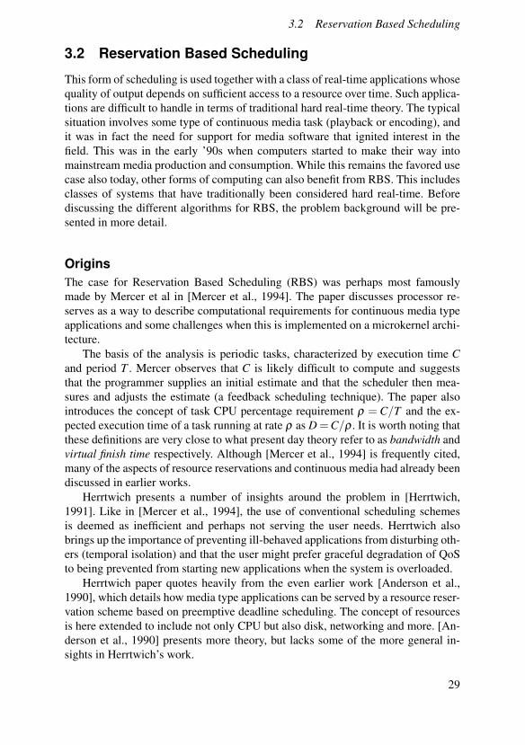
Hierarchical Scheduling StructuresOne desirable property in consumer grade systems is to be able to mix real-timeapplications with regular applications. Often this leads to a construction with a hi-erarchy of schedulers, typically with some hard-real time scheduler on top and softreal-time and regular best-effort schedulers underneath. [Xingang et al., 1996] sug-gests using a tree structure where each node is either a scheduler node or a leafnode. Parents schedule their children until leaf level, where the regular tasks sit,is reached. An example is provided in Figure 3.1. The paper also describes a vari-ant of WFQ called Start-time Fair Queuing (SFQ) that provides better guarantee offairness if the amount of available processing power fluctuates over time.
The hierarchical approach to scheduling is also proposed by other groups. TheRTAI/Xenomai extensions to Linux runs a RT-scheduler as root and the Linux op-erating system as a thread (see Section 3.7). The structure is similar to the oneproposed in [Xingang et al., 1996]. The Bandwidth Server class of RBS algorithms,
30

3.2 Reservation Based Scheduling
root(SFQ)
Hard RT(EDF)
Soft RT(SFQ)
BestEffort
User 1 User 2
Figure 3.1 Hierarchical structure with schedulers. Note that SFQ is used on morethan one level.
detailed in Section 3.2, also uses a hierarchy of schedulers, typically with an Ear-liest Deadline First (EDF) scheduler [Buttazzo, 1997] on top. Hard real-time tasksare scheduled directly by the EDF algorithm, while soft real-time tasks have ded-icated "servers" that dynamically set their deadlines to achieve CPU reservations.Regular applications can be scheduled by a separate server. Lipari et al presented ahierarchical Constant Bandwidth Server construct called the H-CBS in [Lipari andBaruah, 2001] in 2001.
The choice of top level schedulers becomes more critical in the case of insuffi-cient resources. Fixed priority schedulers favor high priority tasks while EDF sched-ulers will spread out the effects [Cervin et al., 2002] [Buttazzo et al., 1995].
Bandwidth ServersThe concept of bandwidth servers was derived from Dynamic Priority Servers(DPS) by Buttazzo [Buttazzo, 1997]. DPS is a method to accommodate aperiodicor sporadic tasks in fixed priority systems, essentially through a hierarchy of sched-ulers. The Priority Server is a periodic task with a specified execution time. Arrivingaperiodic tasks are placed in a queue and executed by the Priority Server when it isscheduled to run. In the original formulation, unused capacity is just lost.
Buttazzo brought the concept of a server presiding over a predetermined amountof CPU capacity to the dynamic scheduling algorithms. The Dynamic Priority Ex-
31
Chapter 3. Reservation based scheduling
change Server (DPE) and the Total Bandwidth Server (TBS) [Spuri and Buttazzo,1996] were the first formulations using EDF as a root level scheduler. The objectivewas still handling aperiodic tasks and a lot of theory concerned handling of unusedbandwidth. In 1998, Buttazzo and Abeni published [Abeni and Buttazzo, 1998b],which introduces the Constant Bandwidth Server (CBS). By then, the Continu-ous Media (CM) problem had already been addressed using the Bandwidth Servermetaphor by [Kaneko et al., 1996].
Constant Bandwidth ServerThe CBS formulation is a popular construct for software reservations and is ex-plained further in this section.
Consider a set of tasks τi where a task consists of a sequence of jobs Ji, j witharrival time ri, j. Let Ci denote the the worst case execution time (WCET) in thesequence and Ti the minimum arrival interval between jobs. For any job, a deadlinedi, j = ri, j+Ti is assigned.
A CBS for the task τi can then be defined as:
• A budget, cs, and a pair (Qs,Ts) where Qs is the maximum budget and Tsis the period. The ratio Us = Qs/Ts is called the server bandwidth. At eachinstant, a fixed deadline, ds,k, is assigned to the server with ds,0 = 0.
• The deadline di, j of Ji, j is set to the current server deadline ds,k. If the serverdeadline is recalculated, then so is the job deadline.
• When a job associated with the server executes, cs is decreased by the sameamount.
• When cs = 0 the budget is replenished to the value of Qs and the deadline isrecalculated as ds,k+1 = ds,k +Ts. This happens immediately when the budgetis depleted, the budget cannot be said to be 0 for any finite duration.
• Should Ji, j+1 arrive before Ji, j is finished, it will be put in a FIFO queue.
Variations on the CBS formulationCBS-hd This reformulation of the replenishment rule makes it possible for veryoverrun sensitive applications to get access to parts of its budget on a shorter dead-line. This is investigated in [Caccamo et al., 2000].
The Control Server (CS) Cervin and Eker presented in [Cervin and Eker, 2003]a modification to the CBS scheme that would make it easier to handle the timingneeds of a control application. The server budget cs is here spread out over a numberof smaller segments, reducing the uncertainty as to when an input will be read, anoutput be set, or a code function executed.
32
3.2 Reservation Based Scheduling
Fair QueueingFairness was originally introduced by Nagle in [Nagle, 1987] using an informaldefinition saying simply that a fair algorithm divides the resources between peersequally. The paper also includes what is essentially a prototype of the WFQ al-gorithm but with little formalism. [Demers et al., 1989] builds on [Nagle, 1987],providing formal definitions and analysis. An algorithm for dividing a resource isdefined as fair if
• no user receives more than its request,
• no other allocation scheme satisfying the first condition has a higher mini-mum allocation and
• the second condition remains recursively true as we remove the minimal userand reduce the total resource accordingly
For applications, the conditions can be expressed in another way. Assume the exis-tence of a finite resource D and n users of that resource. Each user "deserves" a fairshare equal to D/n of this resource, but is allowed to ask for less, in which case thedifference can be allocated to a user who would like more. Let di denote the sharea user requests and ai the share he is given. The maximally fair allocation is thendefined so that the share d f is computed subject to the following two constraints:
n
∑i=1
ai = D (3.1)
ai = min(di,d f ) (3.2)
To quantify the fairness of an measured allocation {a1,a2, ...} compared to themaximally fair allocation {A∗1,A∗2, ...}[Jain et al., 1984] proposes to use a fairnessfunction
Fairness =(∑n
i=1 xi)2
n∑ni=1 x2
i(3.3)
usually referred to as Jain’s Fairness Index, where xi = ai/A∗i . The fairness will bebetween 0 and 1, where 1 represents a maximally fair allocation.
Using this metric, we can discuss how fair an algorithm is, how quickly itachieves it, and how sensitive it is to fluctuating conditions. More notions of fair-ness does, however, exist. The formulation above is limited to calculating the overallfairness, but is difficult to apply to specified time intervals. For that, we need a moreadvanced formulation. In [Golestani, 1994], Golestani introduces a notion of fair-ness based on the concept of normalized service. Let ri be the service share allocatedto a task τi and Wi(t) the aggregate amount of service this task has received in theinterval [0, t). The normalized service is then wi(t) = 1
riWi(t). An algorithm is then
considered fair in an interval [t1, t2] if
wi(t2)−wi(t1) = w j(t2)−w j(t1) (3.4)
33

Chapter 3. Reservation based scheduling
or, in a more compact notation,
∆wi(t1, t2)−∆w j(t1, t2) = 0 (3.5)
for any two tasks τi and τ j that have enough work to execute during the entireinterval and fair if this is true for any interval.
Unless work is infinitely divisible and all tasks can be serviced simultaneously,all scheduling algorithms relying on resource multiplexing will be unfair if t2− t1 ischosen sufficiently small. The theoretical case that allows t2− t1 to go towards 0 iscalled fluid resource sharing and is discussed in [Parekh and Gallager, 2007], thatanalyzes the Generalized Processor Sharing algorithm (GPS). Note that GPS wouldbe completely fair given both definitions of fairness.
Variations of WFQWhile simple in concept, WFQ suffers from being computationally expensive andsensitive to fluctuating resource availability. Several alterations to the original al-gorithm have been proposed to reduce these problems. For instance, the Start-timeFair Queueing approach mentioned earlier was introduced in [Xingang et al., 1996]as one way of increasing robustness to resource fluctuations, while the Self-clockedFair Queuing scheme [Golestani, 1994] removes the need to explicitly calculate theideal processor sharing solution.
The Completely Fair Scheduler The Completely Fair Scheduler (CFS) is a Linuxscheduler that was introduced by Ingo Molnar in the 2.6.23 release of the kernel.The scheduler is called "The Completely Fair Scheduler", but the design documentrecognizes that absolute fairness is impossible on actual hardware. The schedulingprinciple is simple, each task is given a wait_runtime value which represents howmuch time the task needs to run in order to catch up with its fair share of the CPU.The scheduler then picks the task with the largest wait_runtime value. On ansystem with Fairness Index 1, wait_runtime would always be 0.
The implementation of this is slightly less simple. Each CPU maintains afair_clock which tracks how much time a task would have fairly got had it beenrunning that time. This is used to timestamp the tasks and then to sort them, us-ing a red-black binary tree, by the key fair_clock - wait_runtime. Multicorescheduling is supported though a partitioned scheduling scheme, with penalties formigrating to other CPUs. Weights are also used, but as is common in POSIX sys-tems they are called nice levels and have the reverse meaning (a nice process wouldhave a low weight). wait_runtime is also constrained so that heavy sleepers willnot lag too far behind.
In subsequent patches, the group scheduling framework was introduced. Inshort, it is a hierarchical scheduling scheme where the run queue can be made up ofboth individual tasks and groups of tasks. The initial intent was to allow fair sharingof the CPU between users rather than tasks. However, the introduction of control
34

3.2 Reservation Based Scheduling
groups (see below) made it possible to do arbitrary groupings, thereby making it asimple but flexible tool for CPU reservations.
At the time the CFS was being merged into the kernel mainline, there wereseveral competing initiatives to bring reservations to the Linux scheduler. The win-ning patch-set introduced control groups, a general system for grouping tasks andannotating the groups with parameters. These parameters could then be used byvarious kernel subsystems without the need to change the POSIX task model. It isimportant to note that control groups in themselves do not alter the behavior of thesystem, they are just an organizational tool. It is up to the respective subsystems tothen interpret the parameters. Some examples of control group-aware subsystemsare
• the CFS Group scheduler,
• the CPU affinity subsystem ("cpusets"),
• the group freezer (suspends all tasks in the group) and
• resource accounting.
Adding new control group-aware subsystems is at the time of writing the preferredway to introduce new user controllable functionality in the kernel, instead of addingnew system calls.
Comparison between CBS and FQHaving introduced both the bandwidth server and fair queuing approach to RBS,we can now compare the two methods and see how they differ. Such a comparisonis presented in [Abeni et al., 1999], which is summarized here.
First we take a look at the interface they provide for reserving bandwidth. TheCBS dedicates an absolute share while FQ uses relative shares. FQ can emulateCBS but with the need to dynamically recalculate the weights when a new task isadmitted. FQ algorithms also typically provide bounds on delay, which can be seenas a bound on what deadline requirements a new task can pose. Both schemes havebeen extended with feedback to adjust weights or bandwidth to achieve some QoSset-point. On the other hand, FQ can more easily be used with mixed real-time andnon-real-time tasks.
The run-time properties of the algorithms are also different. CBS does not usequantified time which makes its performance more consistent over varying hard-ware platforms. FQ is on the other hand simpler to implement. FQ enforces fairnessat all times while CBS only guarantees bandwidth allocations between deadlines,making it less conservative. The paper makes the case that FQ is not suitable for me-dia applications as it lacks the notion of task period or deadline, but one can arguethat the maximum lag property of an FQ algorithm is a global deadline guarantee,shared by all tasks currently in the system. It is, however, true that the maximum lag
35

Chapter 3. Reservation based scheduling
often depends on the number of tasks in the system and the distribution of weights,making the temporal isolation property of FQ weaker. The paper also states that FQwould generate many context switches in order to enforce fairness. While CBS willhave context switches as a function of the smallest period server, FQ uses a fixedscheduler time quanta for all tasks. However, as seen with, e.g., the Completely FairScheduler, scheduling allowances can be worked in to reduce the number of contextswitches, at the cost of worse moment-by-moment fairness.
Latency-Rate ServersIn [Stiliadis and Varma, 1998], a generalization of different FQ algorithms are pro-posed. The class of schedulers called Latency Rate servers (LR-servers) are definedas any scheduling algorithm that guarantees that an average rate of service offeredto a busy task, over every interval starting at time Θ from the beginning of the busyperiod, is at least equal to its reserved rate. Θ is called the latency of the server. Alarge set of the FQ algorithms fit into this class, including WRR, WFQ and SCFQ.Even non-fair algorithms can qualify (one such example presented in the paper isthe Virtual Clock algorithm [Zhang, 1990]).
[Stiliadis and Varma, 1998] goes on to derive a number of results for this rathergeneral class of schedulers, including delay guarantees and fairness bounds. Oneinteresting result is that a net of LR-servers can be analyzed using one equivalentsingle LR-server. This can be useful when considering a hierarchy of schedulers.
Alpha-Delta abstractionSimilar to the LR-server formulation is the Alpha-Delta abstraction proposed in[Mok et al., 2001b]. Bounds for minimum service α and delay ∆, corresponding torate and latency in the LR-server formulation respectively, are here derived from areal-time scheduling point of view.
3.3 Feedback allocation control
Adaptive ReservationsOne problem when doing RB scheduling is that the execution time for a periodictask may vary over time. As it is undesirable to base our calculations on the worstcase, it is likely some deadlines will be missed. While the CBS scheme can handletransient overruns, non transient changes will lead to eventually infinite deadlines(instability). One way to remedy this would be to dynamically set the budget for aserver based on prior overrun statistics in a feedback control manner, though com-monly referred to as adaptivity in computer science publications.
In [Abeni and Buttazzo, 1999], Abeni and Buttazzo introduce a metric called thescheduling error. If we have a periodic task τi with period Ti, then the schedulingerror εs is defined as
εs = ds− (ri, j +Ti), (3.6)
36

3.3 Feedback allocation control
i.e., the difference between the server deadline and the soft deadline of the task.Feedback using the server budget Qs as the control signal would then be used todrive εs towards 0.
A few design techniques for such a controller are discussed in [Marzario et al.,2004]. For the purpose of making the analysis simpler, a restriction is imposed sothat even if there is extra unused bandwidth available, a task τi scheduled by a CBSwill only receive the bandwidth Qs, a so called hard reservation. Assume that τi is aperiodic task being served with a CBS, divided into jobs Ji, j with the correspondingrelease times ri, j. This gives ri, j+1 = ri, j +Ti, where Ti is the task period. Each jobis associated with a soft deadline di, j = ri, j +Ti, that is di, j = ri, j+1. Let fi, j be theactual finish time for Ji, j and vi, j be the finish time had τi been running alone on aCPU with the fraction bi = Qs/Ts of the actual CPU speed, i.e., the virtual finishtime. The article uses a modified definition of the scheduling error compared to 3.6
εi, j = ( fi, j−1−di, j−1)/Ti (3.7)
which is the scheduling error experienced for Ji, j−1. Note that since hard reserva-tions is being used, having both ε j > 0 and ε j < 0 is undesirable since the taskwould either be missing deadlines or wasting bandwidth. The relation
vi, j−δ ≤ fi, j ≤ vi, j +δ (3.8)
where δ = (1− bi)Ts, tells us that we can make the CBS approximate the GeneralProcessor Sharing (GPS) algorithm by letting Ts go towards 0. Even with normalchoices of Ts it is reasonable to use 3.7 and 3.8 to approximate the scheduling errorwith
ei, j = (vi, j−1−di, j−1)/Ti (3.9)
A difference equation for the evolution of the scheduler error is then presentedin [Abeni et al., 2002]. The paper also proposes a predictor based control structureand three examples of control design using invariant based design, stochastic deadbead design and optimal cost design respectively.
Real-Rate SchedulingOne of the first examples of rate-based scheduling was proposed in [Goel et al.,2004]. The novel approach is to use some task output to measure the rate of progressand thereby eliminate the need for the software designer to assign deadlines or CPUshare directly. Experiments presented in the paper are performed using a slightlymodified Linux 2.0 series kernel augmented with an rate monotonic scheduling-based RBS scheme. A task with no known period or CPU share requirements but ameasurable progress is in [Goel et al., 2004] called a real-rate task.
The example studied is a video pipeline with a producer and a consumer thatexchange data via a queue. Queue fill level is the metric used for progress. Thescheduler samples the queue and decides if either of the two is falling behind or
37

Chapter 3. Reservation based scheduling
getting too far ahead. They use a half-filled queue as the set-point and then designa PID controller to decide the CPU share needed. The period is decided using anheuristic based on the size of the share, lower share meaning longer period.
HeartbeatRate-based allocation is further supported by the Heartbeat framework [Hoffmannet al., 2010], which proposes instrumentation of applications so that significantevents can be detected by the resource reservation framework. The framework pro-vides an API for registering applications with the resource manager and specifyingrate and latency set points. Rates are estimated from events using sliding windowmethods but individual time stamps of events are saved in order to facilitate morein-depth analysis.
A Linux-based implementation is presented together with results from experi-ments on a number of application types, including image analysis and video play-back.
3.4 Allocation
With the establishment of a variety of RBS techniques, the next important ques-tion to discuss is how to calculate the reservations. Given a set of timing sensitiveapplications, individual application performance can be sacrificed to obtain betterglobal performance. The theory of splitting a resource between consumers is of-ten called resource allocation, though considering its mathematical properties, con-strained control would be just as accurate.
Within the field of operations research, using optimization to solve logisticsand resource allocation problems is common practice. Some of the iconic prob-lems have been formulated here, including the knapsack and bin packing problems.Solving knapsack- and bin packing problems exactly is of NP-complete complexity[Kellerer et al., 2004; Coffman et al., 1997], making them unattractive for on-lineuse in limited computational capacity settings.
Constrained control theoryA popular tool for managing constrained dynamics in control is the Model Pre-dictive Control (MPC) formulation. The default setup is postulating a convex costfunction of the state trajectories, using an LTI-model as trajectory constraints [Ma-ciejowski, 2002]. Though mathematically feasible to use for allocation problems,solving convex optimization problems can be very resource demanding if specialcare is not taken.
The Explicit MPC formulation uses pre-calculated solutions, thereby convert-ing computational complexity to a need for storage space. As a result, optimiza-tion problems typical for MPC can be solved in milliseconds [Zeilinger et al.,2009; Geyer, 2005]. Calculations can be sped up even further using hardware-based
38

3.5 Reservation frameworks
solvers generated from the problem description, as shown in [Jerez et al., 2012].The assumption that problem structure is known and fixed does, however, makepre-computed solutions impractical for dynamic resource allocation.
Another way of obtaining very fast and efficient solvers is to generate special-ized solvers based on the problem formulation. The CVXGEN package is specifi-cally targeted at embedded platforms, but does not support fixed point arithmeticsand is limited to linear- and quadratic programming problems [Grant and Boyd,2010; Mattingley and Boyd, 2012].
Parallelizing solvers and making it possible to obtain at least partial results be-fore the optimization has terminated are other approaches that can be useful whensolving optimization problems in real time. [Giselsson et al., 2013] presents a dis-tributed gradient-based algorithm that uses short iterations together with conver-gence rate results.
Q-RAMIn 1997, R. Rajkumar presented his Quality-of-Service-based resource allocationmodel, Q-RAM [Rajkumar et al., 1997]. In essence, this states the allocation as asingle objective constrained optimization problem. The model as it was introducedallowed for multiple tasks using multiple resources. Tasks are given utility functionsbased on the allocated resources, but no technique for how to model a specific task ispresented. Neither is the problem of solving constrained optimization problems on-line discussed. In a later paper [Saewong and Rajkumar, 1999], Rajkumar suggestsone way of overcoming the NP-hard problem of general multi-resource allocation,but neither this paper discusses the algorithmic properties of the problem in detail.
3.5 Reservation frameworks
OCERAOCERA [OCERA 2010] stands for Open Components for Embedded Real-time Ap-plications, and was a European project, based on Open Source, which provided anintegrated execution environment for embedded real-time applications. From a RBSpoint of view, OCERA offers a number of interesting components. The OCERAcode is based on the RTLinux extension. The patches are applicable to Linux ker-nels up to version 2.4.18.
Scheduler Patch OCERA modified the Linux kernel so that it provided "hooks"for modules implementing generic scheduling policies. The patch used for this iscalled the Generic Scheduler Patch (GSP), intended to modularize the scheduler partof the kernel so that additional scheduler policies could be added without furthermodification to the kernel source.
Integration Patch The Preemptive Kernel Patch is made to work with RTLinuxusing OCERA’s Integration Patch. The Preemptive Kernel work was done by Robert
39

Chapter 3. Reservation based scheduling
Love with the aim of improving latency by making system calls possible to preempt[Rostedt and Hart, 2007].
Resource Reservations Scheduling module A dynamically loadable kernel mod-ule that provides a resource reservation scheduler for soft real-time tasks in userspace is distributed with the OCERA components. It uses a CBS-based algorithm,modified to handle some practical issues. It includes optional slack reclamationfunctionality using the GRUB algorithm. The module provides a new schedulingpolicy, SCHED_CBS.
Quality of Service Manager OCERA also provides a QoS management servicesmodule. This is more or less a controller which changes the bandwidths accordingto the scheduling error. The approach is more or less that presented in Section 3.3.
AQuoSAAQuoSA [AQuoSA 2010] stands for Adaptive Quality of Service Architecture and isanother initiative to bring QoS to the Linux kernel. It builds on the work provided byOCERA and was partially sponsored by the European FRESCOR project. Structure-wise AQuoSA retains the components used by OCERA. AQuoSA has adopted theIRMOS scheduler, a hierarchical EDF-based scheduler described further in Section3.5.
FRESCORFRESCOR [Harbour, 2008] (Framework for Real-time Embedded Systems basedon COntRacts) focuses on hard-realtime and contract based resource management.The project background is similar to that of this thesis, dealing with the problem ofunknown execution times, mixed requirements and maximizing resource utilization.
The idea is to automate much of the real-time analysis by exposing an API in theform of service contracts. Once the user has specified the requirements, the platformnegotiates all current contracts to see if there is a valid solution.
A contract is a set of attributes describing the resource needs of the applicationas well as certain application properties. Some central concepts here are
• resource type (e.g., process, network or memory),
• minimum budget (WCET/T),
• maximum period, and
• deadline.
These parameters are then used for automated response time analysis to determineif the resource requirements can be met.
40

3.5 Reservation frameworks
Spare capacity distribution In order to address the goal of maximum resource uti-lization, FRESCOR suggests a form of slack reclamation here called Spare capacitydistribution (SCD). As the admission policy works under worst case assumptions,it is likely the system will have spare capacity in most situations.
ACTORSACTORS (Adaptivity and Control of Resources in Embedded Systems) was a Eu-ropean Union funded research project with the goal to address design of resource-constrained software-intensive embedded systems. The strategies employed in-cluded
• data flow-based programming and code generation,
• virtualization and
• feedback resource management.
One of the primary deliverables from the project was an implementation of an adap-tive resource management framework [Bini et al., 2011].
ACTORS-model In [Segovia and Årzén, 2010] the authors present a model, us-ing a set of discrete resource consumption and quality output levels. The problemformulation concerns both assigning tasks to cores and dimensioning resource reser-vations for each core. The domain mentioned as the target in the paper is data-flowapplications, but there is nothing explicitly in the model that ties it to this.
One drawback of this approach is the need to supply the resource levels. This isnon-trivial and increases the complexity of developing applications. The approachtaken in the paper requires only one defined level and utilizes a continuous qualitymeasure, thereby making the optimization easier to solve.
Figure 3.2 shows an architectural overview of the actors resource managementmodel, where a physical platform is virtualized and presented as a number of re-source constrained virtual platforms to the applications layer. The architecture sup-ports mapping one CPU core into many virtual cores, but while multicore systemsare supported the model does not allow for a virtual resource to stretch over manyphysical.
The resource manager (RM) allocates virtual platforms to applications as theyrequest resources and monitor the application performance in runtime in order toadapt resource levels for optimum system performance. Each RM aware applicationis designed with a number of predetermined Service Levels (SL), each correspond-ing to a nominal resource demand and performance.
The problem of assigning virtual platforms to actual hardware and selectingservice levels for all running applications is posed as a mixed integer programmingproblem and solved using the GNU Linear Programming Kit [GLPK]. This was
41
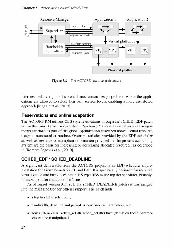
Chapter 3. Reservation based scheduling
Figure 3.2 The ACTORS resource architecture.
later restated as a game theoretical mechanism design problem where the appli-cations are allowed to select their own service levels, enabling a more distributedapproach [Maggio et al., 2013].
Reservations and online adaptationThe ACTORS RM utilizes CBS style reservations through the SCHED_EDF patchset for the Linux kernel, as described in Section 3.5. Once the initial resource assign-ments are done as part of the global optimization described above, actual resourceusage is monitored at runtime. Overrun statistics provided by the EDF-scheduleras well as resource consumption information provided by the process accountingsystem are the basis for increasing or decreasing allocated resources, as describedin [Romero Segovia et al., 2010].
SCHED_EDF / SCHED_DEADLINEA significant deliverable from the ACTORS project is an EDF-scheduler imple-mentation for Linux kernels 2.6.30 and later. It is specifically designed for resourcevirtualization and introduces hard CBS type RBS as the top tier scheduler. Notably,it has support for multicore platforms.
As of kernel version 3.14-rc1, the SCHED_DEADLINE patch set was mergedinto the main line tree for official support. The patch adds
• a top tier EDF scheduler,
• bandwidth, deadline and period as new process parameters, and
• new system calls (sched_setattr/sched_getattr) through which these parame-ters can be manipulated.
42
3.6 The Xen hypervisor
The implementation does have multicore support, but the official documentationincluded with the initial release states that some issues around task migration stillremains to be resolved.
The inclusion of a true EDF scheduler and support for CBS style reservations inthe Linux kernel can mean a great deal to wide spread adoption of reservation basedscheduling in consumer products and general computer systems, as such function-ality has historically only been available in research grade software or expensiveproprietary operating systems.
IRMOS SchedulerThe IRMOS scheduler [Cucinotta et al., 2011], developed by the EU funded projectInteractive Realtime Multimedia Applications on Service Oriented Infrastructures,is a hierarchical scheduler patch for the Linux kernel with many similarities toSCHED_DEADLINE, but with two notable features. First of all, it is a hierar-chical scheduler that permits other schedulers to be run inside it. Secondly, whileSCHED_DEADLINE is a partitioned EDF scheduler, IRMOS has an experimentalglobal EDF implementation.
3.6 The Xen hypervisor
Virtualization technologies make it possible to partition a physical computer intoseveral logical instances, each one running a separate operating system that expe-riences itself as running alone on the hardware. The layer beneath the OS layer issometimes called the hypervisor layer as it uses a special mode enabled in modernCPUs called the hypervisor mode. Xen is an open source hypervisor created in 2003at the University of Cambridge [Barham et al., 2003].
ArchitectureA Xen system has multiple layers, the lowest and most privileged of which is Xenitself. Xen can host multiple guest operating systems, each of which is executedwithin a virtual instance of the physical machine, a domain. Domains are scheduledby Xen and each guest OS manages its own applications. This makes up a hierarchyof schedulers with the Xen scheduler on top.
Xen supports several top level schedulers, including EDF and WFQ. This makesit possible to apply resource reservation to the virtual machines running on top ofXen.
3.7 Xenomai
Xenomai [Xenomai 2010] is a real-time development framework cooperating withthe Linux kernel, in order to provide a pervasive, interface-agnostic, hard real-time
43

Chapter 3. Reservation based scheduling
support to user-space applications, seamlessly integrated into the GNU/Linux en-vironment. It is an alternative to RTLinux and RTAI and is a possible platform fordeveloping RBS schemes. It was launched in 2001 and in 2003 merged with theRTAI project. The projects split again in 2005, going after separate goals.
Xenomai achieves superior real-time performance compared to standard Linuxwhile still allowing regular applications. The real-time kernel is a small, efficientrun-time which executes the Linux kernel as a low priority task. Real-time taskswill then be run by the RT kernel, next to the Linux kernel. The Xenomai kernelalso provides an API with extensive support for real-time primitives that the Linuxkernel lack, including support for periodic task models. Xenomai uses a hypervisorsimilar to the Xen hypervisor, but focuses on real-time performance. For example,it allows real-time tasks to receive interrupts even if a Linux process has requestedinterrupts to be turned off.
3.8 Linux Control Groups
The introduction of Control Groups in the Linux kernel provided an extensibleframework for hierarchical organization of processes. The patch came as a responseto a series of patch sets aiming to add resource reservation functionality to the Linuxkernel. Rather than adding more subsystems, the control group patch implementedthe support by extending and generalizing the existing cpusets functionality. Controlgroups extracts the process grouping code from the former cpusets implementationinto a generic container system, and then reimplements cpusets on top of that as oneof many possible modules. The intention is that the various resource managementand virtualization efforts can also become modules rather than separate patch sets,with the result that
• the user space APIs are (somewhat) normalized
• the additional kernel footprint of any of the competing resource managementsystems is substantially reduced, since it does not need to provide processgrouping/containment, hence improving their chances of getting into the ker-nel
Together with the aforementioned group scheduling mechanism introduced in Linux2.6.24 (see Section 3.2), control groups enables a primitive form of resource reser-vations for processes and users.
3.9 Estimating software model parameters
Uncertainty and time varying dynamics can be handled through on-line estimationtechniques, as is common in feedback and adaptive control. For a system with vary-
44

3.9 Estimating software model parameters
ing time scales, both over time and between components, traditional periodic sam-pling will not fit well.
Recently, event based control and estimation has gained attention. Such theoryis attractive because it can be more efficient than periodic sampling and also betteraccount for situations where information is delivered in an event based fashion. Thisthesis has been inspired by such works as [Henningsson and Cervin, 2009; Sandeeet al., 2007].
45
4Power and energymanagement
This chapter introduces prior research related to power management and energymanagement for cyber-physical systems (CPS). The chapter starts with an intro-duction of the problems associated with power management in mobile systems andhow they relate to the resource allocation problems presented in the previous chap-ter. After that follows research related to minimizing power consumption throughscheduling techniques, both for the single core system and computer clusters. Fi-nally some results related to the explicit management of heat dissipation and powerconsumption are presented.
4.1 Energy and resources
In previous chapters, the need for resource management techniques for situationswith time varying resource availability was discussed at length. In mobile systems,the constant attention to energy concerns is perhaps the most important source ofresource variability. Tightly coupled with this is heat management, as all forms ofenergy expenditure invariably leads to the development of heat, the dissipation ofwhich is a problem in all high performance computer environments, mobile or not.
Thermal RC-modelsGiven the limitations on how a mobile device can dissipate heat, having appropri-ate models for describing temperature dynamics within the system is necessary forproper power management. Such models must not only consider how heat is pro-duced through the operation of the system components, but also how it propagatesbetween them. Controlling peak temperatures and temperature gradients thus be-come part of the resource management problem.
A popular model structure used in many papers likens the flow of thermal energyto that of electric currents in a circuit made up of resistances and capacitances. In
46

4.1 Energy and resources
Power usage and
heat dissipation
Resource availability
and consumption
Figure 4.1 In the cyber-physical world, physical and computational dynamics af-fect each other, making it necessary to develop models that can encompass bothaspects.
these models, temperature fills the role of potential from the electric counterpart,whereby thermal energy flows from high temperature nodes to low temperaturenodes, limited by the conductive properties of the connecting medium, modeled asresistances.
The simplest possible model would connect one node with the surroundingmedium. If the temperature in the node is denoted T , the surrounding temperaturedenoted To and the thermal resistance between them denoted R, the resulting heattransfer from the node to the surrounding environment H can be calculated as
RH = To−T (4.1)
The effect of a flow H on a node with temperature T is described through the phys-ical property of thermal capacitance, here denoted C, and obeys the equation
CT = H. (4.2)
Through the application of the thermal equivalents of Ohm’s Laws and Equations4.1 and 4.2, larger structures of thermal RC-circuits can be analyzed, as exemplifiedin [Skadron et al., 2002; Ferreira et al., 2007b]. Though the physical parameters arenot easily derived analytically from known system parameters, the linear structureof thermal RC-models makes it easy to apply techniques of system identification tofind the parameter values.
Adding active elements that consume energy and produce heat consists primar-ily of adding more heat flows. Commonly the CPU is considered to be described
47

Chapter 4. Power and energy management
by two power levels: an idle level and a max load level, with a linear interpolationmodel for loads between 0% and 100%, or formally
PCPU = P0% +U(P100%−P0%) (4.3)
where U denotes the load.[Skadron et al., 2002] marks one of the earliest applications of these models
for heat management in computer systems. Over time the thermal RC-models haveseen much refinement, resulting in advanced simulation packages, such as HotSpot[Skadron et al., 2003].
Thermal control techniquesControlling temperature in relevant nodes of the system can be done through ma-nipulation of the entities in the above equations. The techniques for this fall intomainly two categories, controlling the power used by the system through DynamicVoltage- and Frequency Scaling (DVFS) or by restricting the load through schedul-ing policies or as part of resource management.
Clock gating Clock Gating, sometimes referred to as Global Clock Gating orStop-Go, is a technique for preventing overheating in circuits by stalling the clocksignal when the temperature in the chip rises over a threshold level. This will stopall state changes in latches in the circuit, thereby immediately reducing the amountof heat generated. However, as heat can also come from leak currents and exter-nal sources, this is not always sufficient to prevent the circuit from overheating andtaking permanent damage.
Dynamic Voltage- and Frequency Scaling (DVFS) Intel Corporation introducedits Geyserville (later trademarked as SpeedStep) technology in 1999, bringing vari-able speed processors into the mainstream, enabling a significant gain in battery lifefor laptop computers. Since then, the inclusion of DVFS features has been adoptedby most CPU manufacturers, although under different names and implementations.
In general, flipping latches in the CPU consumes power, so reducing the fre-quency with which this happens reduces the power consumption. As the voltagerequired to power a chip depends on the clock frequency it runs at, reducing fre-quency also enables reduced voltage and as such the techniques are commonly usedtogether [Aydin et al., 2004].
Power aware scheduling The simultaneous treatment of selecting operating volt-age and frequency for a CPU and a schedule for the real-time tasks executing on it,in order to minimize the peak power or energy used by the system, has been treatedin a multitude of publications since the introduction of the technology. Starting withmethods relying on off line analysis [Aydin et al., 2001], the trend has since beensteadily towards making more and more decisions online [Aydin et al., 2004].
48

4.2 Spatial resource management, "E-logistics"
Extensions to multicore computing has since been developed [Bautista et al.,2008] as well as for distributed systems, such as data centers [Laszewski et al.,2009; Sharma et al., 2003].
Controlling the power/performance trade-offAs more dynamic techniques are being developed, it has become natural to considerthe trade-off between power consumption and system performance or Quality ofService (QoS). In [Sharma et al., 2003], the objective is to minimize the energyconsumption while not violating performance constraints. The metric used here iscomputational delay and the constraint is that all tasks admitted to the system shouldmeet their deadlines, i.e., a hard real-time formulation. In essence, the trade-offdecision here becomes if to admit tasks to the system or not.
Other works rely more on user oriented metrics, such as the transaction delayexperienced by the user of the system [Chen et al., 2008]. As these metrics are notformulated in terms of hard deadlines, they are soft real-time systems, somethingwhich has become a staple of power aware computing systems. The fact that the me-dia applications, typically considered as being soft real-time, stand for a significantportion of the resource demand, has eased this transition.
With this increased focus on measurable performance rather than the certifica-tion of hard real-time schedulability has come a noticeable change in paradigm.Using the techniques available through reservation based scheduling, managing thelimited resources and the side effects of their consumption becomes more like tra-ditional process control problems, as discussed in for example [Fu et al., 2010a].
4.2 Spatial resource management, "E-logistics"
The theory of real-time systems traditionally concerns the temporal aspects ofresource management, answering question predominantly concerning "when" tospend resources (and on what). With the introduction of multiprocessor and mul-ticore computing, the notion of locality, "where", is introduced, i.e., the spatial as-pects of the problem. As systems spread out even further, connecting componentsthrough system buses or network protocols, spatial effects grow stronger.
Distributed systems can arise by two primary mechanisms, decomposition ofmonolithic systems or composition of individual parts. What separates a part in adistributed system from another does not have to be space, rather two parts can beconsidered separate if giving a resource to one does not mean it is immediatelyavailable to the other, given some relevant time scale.
Systems on static topologiesA static topology system is one where the structure is explicitly part of the systemdesign. The robot example in Section 2.2 is one such system, where the connections
49

Chapter 4. Power and energy management
between components are represented by physical connections. Other examples in-clude task graphs, networked control systems, and queue systems.
Task graph scheduling For system of purely software components, a popular andwidely researched formulation is that of task graph scheduling. The objective is tomap a set of tasks with precedence constraints onto a set of identical processors, aproblem proven to be NP-complete [Robert, 2011]. This formulation has resultedin numerous heuristic designs, most of them static in nature, which makes them in-feasible for scenarios with high variability in resource availability. Recent work hasmoved towards more dynamic formulations, acknowledging the need to considermore uncertain situations [Choudhury et al., 2012].
Networked control systems A common type of static topology system is net-worked control systems, i.e., where controllers, actuators and sensors are physicallyseparate nodes in a computer network. Since control system performance is stronglydependent on timely measurements and actions, managing limited bandwidth is keyto a successful design. Applying control theory to the joint problem of managingthe resources and the plant is a natural step, studied by, e.g., [Branicky et al., 2002].This would later give rise to the event based control structures discussed by, e.g.,[Tabuada, 2007; Cervin and Henningsson, 2008].
Queue systems Given the similarities between scheduling of processor time andqueue theory as discussed in Chapter 3, it is not surprising to find static topologyresource management problems arising in network engineering and queue systemstheory, though usually referred to as "congestion control", see for example [Aky-ildiz et al., 2001; Katabi et al., 2002]. With the ever increasing demands on costefficiency, it is also expected that more and more dynamic methods are applied inorder to refrain from over-provisioning, as exemplified in [Wang et al., 2010].
Systems on dynamic topologiesA dynamic topology system is one where the structures changes over time, either au-tonomously or driven by decisions. Ad-hoc networks and overlay networks are typ-ical examples of systems with dynamic topologies, but lately the drive for greenercomputing has led to the studies of how to turn of network links in order to saveenergy.
Overlay networks and content distribution Digital media and content distributionare arguably the driving forces behind both technology and legislation relating to theinternet. It is becoming clear that the current infrastructure is not designed aroundthe sustained data rates associated with streaming music and video and as suchservices become increasingly popular, there is a strong demand for technologicalsolutions to reduce congestion and energy consumption.
Peer-to-peer (P2P) and peer-assisted solutions have been used in wired networksto reduce infrastructure load [Kreitz and Niemela, 2010], but as mobile devices are
50

4.2 Spatial resource management, "E-logistics"
increasingly the point of media consumption, there is a strong demand for extendingthese solutions to the mobile networks.
The principal complication in the mobile case is the addition of energy con-straints. While traditional P2P has proven effective for cooperative content distribu-tion and offloading congested nodes or links in the network, it is not energy awareand as such a phone risks running out of power by serving content to others beforeit can benefit from accumulated goodwill.
The study of local cooperative techniques that account for the energy cost ofsharing data has recently been done by several independent groups. Common amongthem is that they leverage the lower energy consumption of short range communi-cation and point out the additional benefit of local schemes in that they offload thelong range infrastructure [McNamara et al., 2008].
[Jung et al., 2010] introduces a framework for cooperative sharing, starting withan altruistic scheme and then introduce guard conditions to prevent participantsfrom spending too much energy on serving content. The approach is based on aMarkov Decision Process (MDP) formulation, which is studied in detailed in [Che-ung et al., 2009], and is validated through an implementation on Android basedphones showing substantial energy savings. One issue with the experimental setupis that the clients involved are assumed to be in contact with each other indefinitely.Additionally, the approach does not guarantee that participants will actually benefitfrom the scheme.
[Jin and Kwok, 2010] considers a streaming scenario using a game theoreticalapproach. The theoretical framework includes both power and bandwidth consider-ations, but simplifies the game dynamics by assuming that players without sufficientenergy will simply not participate. While the real time aspects introduced throughthe streaming scenario are relevant, the formulation is very abstract and it is notclear how it could be implemented in reality.
[Yaacoub et al., 2012] also approaches the problem using a game theoreticalbasis, but explicitly addresses the energy issue and fairness. A large file object isdistributed to a set of clients by transmitting parts of it to some nodes over long dis-tance link and then distributed to the rest using local communication. The proposedscheme permits selecting utility in a variety of ways, including greedy but unfairminimization of the total energy used by the system and minimizing the maximumenergy spent by any client. The proposed solution considers static populations anduses an off-line calculated solution, making it unsuitable for the more dynamic sce-narios studied in this thesis.
51
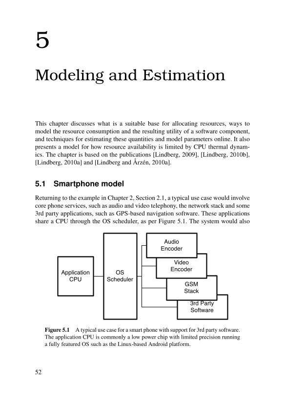
5Modeling and Estimation
This chapter discusses what is a suitable base for allocating resources, ways tomodel the resource consumption and the resulting utility of a software component,and techniques for estimating these quantities and model parameters online. It alsopresents a model for how resource availability is limited by CPU thermal dynam-ics. The chapter is based on the publications [Lindberg, 2009], [Lindberg, 2010b],[Lindberg, 2010a] and [Lindberg and Årzén, 2010a].
5.1 Smartphone model
Returning to the example in Chapter 2, Section 2.1, a typical use case would involvecore phone services, such as audio and video telephony, the network stack and some3rd party applications, such as GPS-based navigation software. These applicationsshare a CPU through the OS scheduler, as per Figure 5.1. The system would also
ApplicationCPU
OSScheduler
3rd PartySoftware
GSMStack
VideoEncoder
AudioEncoder
Figure 5.1 A typical use case for a smart phone with support for 3rd party software.The application CPU is commonly a low power chip with limited precision runninga fully featured OS such as the Linux-based Android platform.
52

5.2 Allocation and utility
be running a number of largely dormant system services that will account for acomparatively small part of the total resource needs.
The arrival of Linux-based smart phones has enabled the use of RBS techniquesto manage performance, rather than by fixed priority scheduling that is the norm.Managing the CPU resource so that software performance is satisfactory can there-fore be seen as an allocation problem.
One complication is that the primary resource, the CPU, is limited in perfor-mance by power and heat constraints. Running software on the CPU produces heatand since most cell phone casings do not support active cooling, the CPU tempera-ture must be regulated by limiting usage.
Given the unknown properties of 3rd party components, the number of combi-nations of enabled software and the varying operational conditions, e.g., ambienttemperature, allocation decisions will have to be made based on information col-lected at runtime.
This chapter will therefore introduce
• a resource consumption and performance model intended for the class of soft-ware components expected to be dominant in terms of resource demands,
• a model describing how available CPU resources depend on chip temperature,and
• techniques for estimating model parameters online.
5.2 Allocation and utility
When allocating a limited resource, it is necessary to consider the utility, some-times called Return On Investment (ROI) or reward, gained. The field of OperationsResearch (OR) is primarily about making such decisions, typically employing con-strained optimization.
Assuming that the applications of interest are timing sensitive rather than hardreal-time, one approach would be to model the utility of an allocation as a functionof the resulting task performance. If hard realtime requirements are assumed, thenotion of individual task performance must be dropped; as a task either performsnominally or fails. Deciding what tasks to admit and which to reject based on theirnominal performance is essentially the knapsack problem, which unsuitability foruse in these contexts has already been discussed in Section 3.4.
Deadline miss ratioUsing the number of task deadlines missed per time interval, Deadline Miss Ratio(DMR), as a measure of utility has been suggested by several previous works, e.g.,[He et al., 2007]. This has been primarily used for feedback resource managementpurposes, but given a model of task execution times, a prediction of the DMR is
53
Chapter 5. Modeling and Estimation
feasible to use. The drawback of such a scheme is that it does not explicitly takeinto account that tasks can adapt to resource availability. This is commonly practicedin modern software, with examples in media processing [Isovic and Fohler, 2004],computer games [Foundry, 2010] and control [Årzén, 1999]. An adaptive task couldtherefore theoretically have the same utility regardless of resource allocation.
Rate-based utilityFor media applications, the quality of the output is strongly connected to the pro-cessing rate. This holds true for all parts of the media processing chain, from encod-ing to decoding. It is therefore natural to consider how resource allocation decisionsimpact the processing rate of the system and thereby indirectly the Quality of Ser-vice. It is possible to view media stream processing as a special case of data flow orstream processing. In these programming models, data is often contained in packetsor tokens which are then processed by a network of computational elements. Therate at which data tokens are processed is a very tangible metric for the applicationperformance. Data flow formulations exist for a large group of software relevant toembedded situations, ranging from automatic control to 3D-graphics. This supportsmaking rate an important basis for resource allocation in heterogenous systems.
Compared with DMR, rate-based utility sets an absolute value to the resultingperformance, though it cannot account for more subtle effects of adaptive tasks.As an example, a video decoder could decide to drop frames as a mechanism forrate adaptation. Deciding which frames to drop is important for playback quality,as discussed in [Cha et al., 2003]. For now, it will be assumed that if a task hassuch properties, it is able to make such decisions by itself. Explicitly including suchinformation in the system global model is in this work considered infeasible for ageneral purpose allocation framework.
Rate is also an application-centric metric which makes it easy to use from adeveloper’s point of view. In many cases the desired execution rate is explicitlydecided at design time, as with encoding frame rate for video, simplifying its useeven further. Given its central position in this work, the term rate deserves a cleardefinition. Rate signifies the number of occurrences of a pre-specified event duringa counting time-period.
The choice of event and counting period is strongly situational. Consider for in-stance the difference between digital audio and video. The ear is much more sensi-tive to audio jitter than the eye is to frame jitter [Steinmetz, 1996]. The audio streamis also sampled at a significantly higher rate than the typical video stream (16 kHzvs 25 Hz). While loosing one or several movie frames during a second might noteven be noticeable for the viewer, loosing the same percentage of audio sampleswill make the audio sound very distorted. When considering a system with mixedtime scales, selecting a suitable time period for allocation can be troublesome. Thiswill be discussed further in Chapters 6 and 7.
54
5.3 Components with rate-based utility
Timing-based utilityAnother alternative is to use the exact time that a task completes a job as a metric, asopposed to whether it always complete ahead of a deadline. This measure containsmore information than the DMR and can be especially useful when co-ordinatingdependent components. An example of this is synchronization between audio andvideo data in a capture device, which is examined in more detail in Chapter 7.
5.3 Components with rate-based utility
This thesis will discuss mostly applications where utility is based on execution ratesand cycle timing. The following section discusses how to model single- and multi-resource dependent components. From a resource consumption point of view, therewill be no difference made between a single- or a multi-threaded process, or evensomething made up from a family of processes. The building blocks will be calledcomponents, where a component i is an entity that
• consumes resources and outputs results opaquely,
• is responsible for distributing allocated resources to subcomponents,
• has a behavior determined by a dynamic mapping from a set of inputs ui to aset of outputs yi, and
• where all significant dependencies affecting performance is modeled throughthis mapping.
There are two main reasons for this:
• Composability. In order to simplify building large systems including 3rdparty components, a building block semantic where the set of parts is closedunder composition is useful. This thesis will disregard the functional aspectsof the component architecture, considering it a mostly solved problem, andfocus on the resource-driven temporal qualities.
• Extending into non-software components. It is the aim of this work tomodel systems built from a mix of software and hardware. Therefore, rais-ing the level of abstraction is necessary to hide properties unique to softwareor hardware parts.
The cyclic component modelThe most basic case is a component that depends on a single resource. In a com-putational setting, this corresponds to the standard problem of a set of independent,CPU-bound tasks. In this work the notions of periods and deadlines are dropped
55

Chapter 5. Modeling and Estimation
+ α(t)∫
ui(t)
vi(t)xi(t) ni(t)
Figure 5.2 A cyclic computation software component. ui(t) is the CPU resourceshare assigned, vi(t) is the disturbance on the assigned share caused by the environ-ment, α(t) is the execution speed of the CPU, xi(t) is the accumulated execution, thelast block is a staircase function mapping xi(t) onto ni(t), which signifies the numberof completed cycles.
and replaced by the notion of cycles. Furthermore, as the entities of interest can bemade up from nested sets of tasks, the term component will be used.
Figure 5.2 shows the logical setup for the cyclic component model, used as thetemplate further on. Generally speaking, the component accumulates the incom-ing resource, in this case executed CPU instructions, until some quantity has beenachieved. At this point it outputs the result and commences a new cycle. The detailsof the model are as follows:
• ui(t) is the CPU resource share assigned to component i and is a dimension-less number.
• vi(t) is a zero-mean disturbance of this share caused by the scheduler as ex-perienced by component i. The two major sources for this disturbance is theerror in the approximation that the CPU is really fluidly divisible and certainsystem events that interrupt normal execution, such as hardware interrupts,virtual memory handling or access of shared resources.
• α(t) denotes the speed at which the processor executes instructions and hasthe unit of completed instructions per time unit.
• xi(t) is the accumulated number of executed instructions for component i.
• ni(t) signifies the number of cycles completed by component i at time t andis calculated as
ni(x) = maxk (5.1)
s.t.k
∑j=1
Ci( j)≤ xi(t) (5.2)
for some sequence Ci(1),Ci(2)...Ci(k) that describes the amount of executionit takes component i to complete computation cycle k.
56
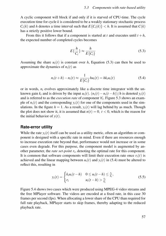
5.3 Components with rate-based utility
A cyclic component will block if and only if it is starved of CPU-time. The cycleexecution time for cycle k is considered to be a weakly stationary stochastic processCi(k) and h denotes a time interval such that E{Ci(k)}< h. It is assumed that C(k)has a strictly positive lower bound.
From this it follows that if a component is started at t and executes until t + h,the expected number of completed cycles becomes
E{ hCi} ≈ h
E{Ci}(5.3)
Assuming the share ui(t) is constant over h, Equation (5.3) can then be used toapproximate the dynamics of ni(t) as
ni(t +h)−ni(t)≈1
E{Ci}hui(t) = hkiui(t) (5.4)
or in words, ni evolves approximately like a discrete time integrator with the un-known gain ki and is driven by the input ui(t). (ni(t)−ni(t−h))/h is denoted yi(t)and is referred to as the execution rate of component Ci. Figure 5.3 shows an exam-ple of ni(t) and the corresponding yi(t) for one of the components used in the sim-ulations. In the figure h = 1. As a result, yi(t) will lag behind by as much. Thoughthe plot does not show it, it is assumed that n(t) = 0, t < 0, which is the reason forthe initial behavior of y(t).
Rate-error utilityWhile the rate yi(t) itself can be used as a utility metric, often an algorithm or com-ponent is designed with a specific rate in mind. Even if there are resources enoughto increase execution rate beyond that, performance would not increase or in somecases even degrade. For this purpose, the component model is augmented by an-other parameter, the rate set-point ri, denoting the optimal rate for this component.It is common that software components will limit their execution rate once ri(t) isachieved and the linear mapping between ui(t) and yi(t) in (5.4) must be altered toreflect this, resulting in
yi(t) =
{kiui(t−h) 0≤ ui(t−h)≤ ri
ki,
ri ui(t−h)> riki
(5.5)
Figure 5.4 shows two cases which were produced using MPEG-4 video streams andthe free MPlayer software. The videos are encoded at a fixed rate, in this case 30frames per second (fps). When allocating a lower share of the CPU than required forfull rate playback, MPlayer starts to skip frames, thereby adapting to the reducedplayback rate.
57
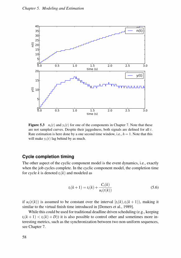
Chapter 5. Modeling and Estimation
0.0 0.5 1.0 1.5 2.0 2.5 3.0time (s)
0
5
10
15
20
25
30
35
40
n(t
)n(t)
0.0 0.5 1.0 1.5 2.0 2.5 3.0time (s)
0
5
10
15
20
y(t
)
y(t)
Figure 5.3 ni(t) and yi(t) for one of the components in Chapter 7. Note that theseare not sampled curves. Despite their jaggedness, both signals are defined for all t.Rate estimation is here done by a one second time window, i.e., h = 1. Note that thiswill make yi(t) lag behind by as much.
Cycle completion timingThe other aspect of the cyclic component model is the event dynamics, i.e., exactlywhen the job cycles complete. In the cyclic component model, the completion timefor cycle k is denoted ti(k) and modeled as
ti(k+1) = ti(k)+Ci(k)
ui(t(k))(5.6)
if ui(t(k)) is assumed to be constant over the interval [ti(k), ti(k + 1)), making itsimilar to the virtual finish time introduced in [Demers et al., 1989].
While this could be used for traditional deadline driven scheduling (e.g., keepingti(k+ 1) < ti(k)+D)) it is also possible to control other and sometimes more in-teresting metrics, such as the synchronization between two non-uniform sequences,see Chapter 7.
58

5.4 Multi-resource dependencies
0.0 0.2 0.4 0.6 0.8 1.0u
0
5
10
15
20
25
30
35
40
y (
fps)
Mean fps for righ-res movie
Piecewise linear approxDatapoints
0.0 0.2 0.4 0.6 0.8 1.0u
0
5
10
15
20
25
30
35
40
y (
fps)
Mean fps for low-res movie
Piecewise linear approxDatapoints
Figure 5.4 Experimental results of controlling CPU-share for the MPlayer decoderusing Linux 2.6.27 and Control Groups. The diagrams show how the frame rate persecond (fps) depends on the amount of CPU share allocated to the decoder. The rateincreases linearly with share until the movie can be played back at encoded rate.
5.4 Multi-resource dependencies
It is desirable to model components that require multiple resources to execute. Thisthesis proposes to do this by extending the component blocking rule so that a com-ponent will block if and only if it is starved of one or more resources. It is assumedthat a component has the capability of accumulating incoming flows, e.g., in FIFOqueues for data or execution time deficit accounting in the scheduler for CPU-time.It follows that the component execution rate is limited by the rate at which resourcesare made available to it. Formally, if τi is dependent on the resource flows u0, ...,uN
yi = min(ki,0u0, ...,ki,NuN) (5.7)
would describe its execution rate. From (5.7) it follows that an allocation strategyshould try to keep the incoming flows equal in order to minimize over-provisioningand reduce the risk of buffer overflow. Furthermore, it points towards two importantobjectives for maximizing performance of these systems:
1. Calculating a steady state flow that maximizes the relevant performance met-ric.
2. Control transient effects that cause blocking .
How Objective 2 is connected to the cycle completion dynamics is further discussedin Chapter 7.
59
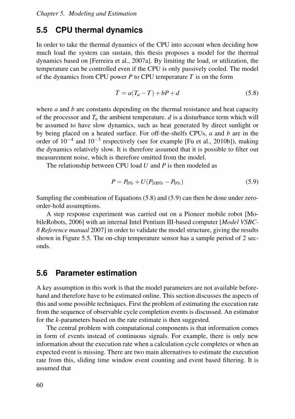
Chapter 5. Modeling and Estimation
5.5 CPU thermal dynamics
In order to take the thermal dynamics of the CPU into account when deciding howmuch load the system can sustain, this thesis proposes a model for the thermaldynamics based on [Ferreira et al., 2007a]. By limiting the load, or utilization, thetemperature can be controlled even if the CPU is only passively cooled. The modelof the dynamics from CPU power P to CPU temperature T is on the form
T = a(Ta−T )+bP+d (5.8)
where a and b are constants depending on the thermal resistance and heat capacityof the processor and Ta the ambient temperature. d is a disturbance term which willbe assumed to have slow dynamics, such as heat generated by direct sunlight orby being placed on a heated surface. For off-the-shelfs CPUs, a and b are in theorder of 10−4 and 10−3 respectively (see for example [Fu et al., 2010b]), makingthe dynamics relatively slow. It is therefore assumed that it is possible to filter outmeasurement noise, which is therefore omitted from the model.
The relationship between CPU load U and P is then modeled as
P = P0% +U(P100%−P0%) (5.9)
Sampling the combination of Equations (5.8) and (5.9) can then be done under zero-order-hold assumptions.
A step response experiment was carried out on a Pioneer mobile robot [Mo-bileRobots, 2006] with an internal Intel Pentium III-based computer [Model VSBC-8 Reference manual 2007] in order to validate the model structure, giving the resultsshown in Figure 5.5. The on-chip temperature sensor has a sample period of 2 sec-onds.
5.6 Parameter estimation
A key assumption in this work is that the model parameters are not available before-hand and therefore have to be estimated online. This section discusses the aspects ofthis and some possible techniques. First the problem of estimating the execution ratefrom the sequence of observable cycle completion events is discussed. An estimatorfor the k-parameters based on the rate estimate is then suggested.
The central problem with computational components is that information comesin form of events instead of continuous signals. For example, there is only newinformation about the execution rate when a calculation cycle completes or when anexpected event is missing. There are two main alternatives to estimate the executionrate from this, sliding time window event counting and event based filtering. It isassumed that
60
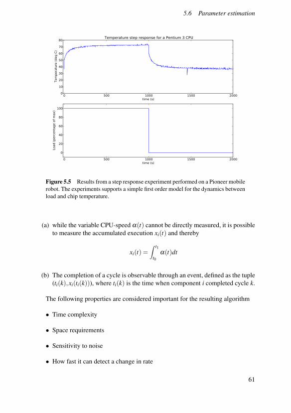
5.6 Parameter estimation
0 500 1000 1500 2000time (s)
0
10
20
30
40
50
60
70
80
Tem
pera
ture
(deg C
)
Temperature step response for a Pentium 3 CPU
0 500 1000 1500 2000time (s)
0
20
40
60
80
100
Load (
perc
enta
ge o
f m
ax)
Figure 5.5 Results from a step response experiment performed on a Pioneer mobilerobot. The experiments supports a simple first order model for the dynamics betweenload and chip temperature.
(a) while the variable CPU-speed α(t) cannot be directly measured, it is possibleto measure the accumulated execution xi(t) and thereby
xi(t) =∫ t1
t0α(t)dt
(b) The completion of a cycle is observable through an event, defined as the tuple(ti(k),xi(ti(k))), where ti(k) is the time when component i completed cycle k.
The following properties are considered important for the resulting algorithm
• Time complexity
• Space requirements
• Sensitivity to noise
• How fast it can detect a change in rate
61

Chapter 5. Modeling and Estimation
Sliding window event countingUsing the definition of rate (events/time period) it is natural to consider an approachwhere the number of events occurring over a predetermined time period is mechan-ically counted. Given a suitable window length, the method is straightforward inimplementation, but needs an unknown amount of memory to keep the events, alsothe time complexity is proportional to the rate, i.e., unknown beforehand.
Event based filteringAn alternative approach is to view the estimation of yi as a prediction problem,where the objective is to at any given time estimate the time between the last andthe yet not arrived event. If ∆(k) = t(k)− t(k− 1), using the assumed stationar-ity stochastic properties of n, a predictor can be written on the discrete time shiftoperator form
∆(k+1) =B(q−1)
A(q−1)∆(k) (5.10)
yi(k) =1
∆(k+1)(5.11)
The selection of the polynomials B and A makes it possible to filter out specificnoise components of the sequence and as long as the filter has unit stationary gain(B(1)/A(1) = 1) the proper mean will be obtained. There is one caveat, however,when dealing with a decreasing rate. If the prediction states that an event shouldoccur but there is none, the estimate must be updated to reflect this. This can bedone through noting that if t time has passed since the last event occurred and t >∆(n+1), then the highest possible current rate would be sustained if an event wouldarrive at the time t+ε . A way to check for this is to tentatively update the predictionas if an event had occurred at the time t and check if the estimated rate would belower. If ∆e(k) denotes the extended sequence {...,∆(k− 1),∆(k),(t − t(k))}, theresulting estimator for y(t) would then be
∆(k+1) =B(q−1)
A(q−1)∆(k)
∆e(k+1) =B(q−1)
A(q−1)∆e(k)
yi(t) =1
max(∆(k+1), ∆e(k+1))
(5.12)
Advantages with this approach is that the filter is fixed in time and space complexity.There is also the added degree of freedom in selecting the filter polynomials Thedownside is that badly chosen polynomials can yield a noisy estimate. By choosingdeg(A) = 1 and deg(B)> 1, the filter gets a finite impulse response (FIR) structure.
62

5.7 Extension into mixed domain models
As this approach has finite memory, just like the time window filter, it is also calledan event window filter. If instead deg(B) = 1 and deg(A) = 1, the structure is calledautoregressive (AR) or infinite impulse response filter (IIR).
k-parameter estimationThe execution rate model given by Equation (5.5) depends on the unknown param-eter k, intended to be to be estimated in runtime. Given an estimate of the currentexecution rate yi(t), falling back on equation (5.5) results in the following estimate:
ki(t) =yi(t)
ui(t−hi)(5.13)
Unfortunately, this estimate does not take the disturbance vi (from Figure 5.2) intoaccount. As it is possible to measure xi(t) directly, a better estimator would be
ki(t) =yi(t)
xi(t1)− xi(t0), (5.14)
if t and t0 and t1 are such that the events used to form yi(t) occur in the interval(t0, t1).
5.7 Extension into mixed domain models
One important objective of this work is to model a system where there is noticeableinteraction between the software components and the hardware components. Theapproach taken is to see it as a system which performance is governed by the flow ofresources. The concept of resource is here extended to mean a quantity, bounded andnon-negative, that through a system component is converted into another resource.The system performance is then expressed in terms of this transformation.
A resource flow is the exchange of a resource between two components of thesystem. In a CPS, a flow can be physical (e.g., heat or power) or virtual (computa-tions or data). In this work physical flows are considered to be L2 functions whilevirtual flows are either L2 or a sequence of Dirac-spikes, with finite density. For-mally, let U denote the set of generalized functions on R such that if u(t) ∈U and,t1, t2 ∈ R then ∫ t2
t1u(t)dt (5.15)
exists and has the sign of t2−t1. The rationale behind resource flows as Dirac-spikesis the event-like manner in which many important virtual resources are generated.As an example, let nCPU (t) denote the number of completed instructions in a CPUand ntask(t) the number of times a sporadic task running on that CPU has executed.Obviously, ntask(t) depends on nCPU (t). In order to analyze the performance of thetask, e.g., to check if it completes cycle n before a certain time, it is necessary to
63

Chapter 5. Modeling and Estimation
PhysicalSystems
SoftwareSystems
ContinuousDynamics
DiscreteFlow
DynamicsEvent
Dynamics
Figure 5.6 A diagram showing how the domains of physical and software systemshave their own unique dynamics, but share the discrete flow dynamics.
study how ntask(t) and nCPU (t) evolve over time, but due to their staircase nature, ift0 denotes some specific time,
limh→0
ntask(t0)−ntask(t0−h)h
(5.16)
is either 0 or undefined. Therefore the dynamics of a system involving virtual flowsmust be expressed in discrete time, here called a discrete flow dynamic.
Forming such a model for physical systems can be done through sampling. Notehowever that while the sampled system description says nothing about the systembehavior between sample points, signals like nCPU (t) and ntask(t) are defined for allt. Because of this, it is possible to talk about exactly when the changes in n occur.
To summarize, the dynamics of a physical system is often modeled throughdifferential equations. These can be discretized or sampled to give a discrete timemodel. Software system are usually modeled through event-based dynamics, butthese can be re-formulated as discrete flow dynamics, comparable with the dis-cretized continuous model. This gives a common model domain with which to ex-press the entire system dynamics. Figure 5.6 shows how the two domains and thedynamic descriptions relate. How such a combined model can be used for resourcemanagement is explored further in Chapter 7.
64

6Competitive resourcemanagement
Chapter 5 presented the performance of the system expressed in two primary met-rics, execution rate and event timestamps, both dependent on allocated resources.This chapter introduces allocation through convex optimization as a way to maxi-mize system performance in the execution-rate sense. A specialized allocation al-gorithm targeted at embedded real-time systems is presented together with a discus-sion about its convergence properties and real-time behavior. This chapter is basedon the papers [Lindberg, 2009; Lindberg, 2010b; Lindberg, 2010a].
6.1 Allocation under resource constraints
The purpose of resource management is to maximize system performance, a non-trivial task when there is not enough resources to run all components at nominalexecution rates. In the terminology introduced in Chapter 5, it is to be expected thatwe cannot keep the rate error of all components at zero, but have to compromise. Toevaluate such a compromise, a global performance metric is needed. For the set ofindependent components, a natural choice would be an aggregate of the individualutility functions. The selection of such an aggregate is an important design parame-ter, which can be used to achieve a compromise suitable to the primary system usecases. For example, it can make sense to prioritize system services over 3rd partycomponents or minimizing the worst case rate error.
In this thesis, it will be assumed that the system performance objective is on theform
J(u) =N
∑i=1
Ji(ui) (6.1)
where Ji is the contribution from component i. In the presence of a resource con-straint, ∑ui ≤U , and under the assumption that resources are positive quantities,
65

Chapter 6. Competitive resource management
the allocation problem can be posed as an optimization problem
minimizeu
N
∑i=1
Ji(ui)
subject toN
∑i=1
ui ≤U
ui ≥ 0,∀i
(6.2)
Convex allocation problemsIn order to find efficient and reliable ways to solve the allocation problem online,i.e., without human supervision, (6.2) needs to be restricted. By limiting the com-ponent contributions Ji to differentiable convex functions, the resulting form willqualify as a convex optimization problem [Boyd and Vandenberghe, 2004]. Thisformulation has has several attractive properties:
• it will always be a feasible problem,
• it will have a unique solution,
• powerful theory exist for designing solvers, and
• it allows for general forms of system utility functions.
Recall the definition of the steady state rate error from Section 5.3:
ei(ui) = ri− yi = ri− kiui. (6.3)
Since Equation (6.3) constitutes an affine mapping, any Ji taken as a the composi-tion of a convex function and ei(ui) will also be convex [Boyd and Vandenberghe,2004, p. 79]. For example, ei(ui)
4 and |ei(ui)| would be viable choices for Ji. Con-ceptually, this means that the problem becomes distributing the rate error rather thanthe resources.
When designing the objective function, some attention should be given to itssensitivity to parameter changes. Since parameters will be estimated online undernoisy circumstances, adopting an linear programming-style objective can lead tosudden jumps in the solution. See [Maciejowski, 2002, p. 151] for a discussion onthe merits of linear and quadratic objectives.
Disabling componentsFor some components performance is only tolerable when yi is close to ri. For thispurpose a lower rate bound y′i can be introduced, which represents the lowest rele-vant execution rate. It would then be desirable to allocate resources so that all com-ponents (if possible) are within their respective regions of tolerable performance. If
66

6.2 Incremental optimization
this is not possible, low priority components must be disabled until
N
∑i=1
y′iki≤U. (6.4)
Solver designThough parameters in this system might not change often, events such as the recon-figuration of an application, the arrival or deactivation of a component or a changein CPU resource availability in response to risk of overheating might require thatwe quickly redistribute resources. Therefore, an algorithm suitable to solving (6.2)online is needed. More specifically, it is desirable that it
1. takes minimal system resources,
2. accounts for changing parameters as quickly as possible,
3. produces results in deterministic time and memory,
4. can improve upon a previous allocation even if aborted before optimum wascomputed, and
5. is suitable for implementation in fixed point arithmetics.
6.2 Incremental optimization
This section proposes an algorithm which can solve (6.2) efficiently and with de-sirable time and memory characteristics. The central idea of the algorithm is to seethe solution as a sequence of resource transfers between two components, in effectsolving the problem as a series of one-dimensional problems. The benefit of thisapproach is that each step is computationally inexpensive, predictable in executiontime and has numerical properties well suited for fixed point implementations.
The problem structure is very similar to the water filling approach to powerdistribution seen in the communications literature, see for example [Boyd and Van-denberghe, 2004], as illustrated in Figure 6.1. Essentially, the components are rep-resented by a set of connected "tubes", with dimensions so that if the tube is filledwith a quantity of water ui, the resulting surface level will correspond to the valueof the marginal utility function Pi(ui) = ∂Ji/∂ui. For the example in Figure 6.1,Ji(ui) = (ri− kiui)
2,∀i. In this case the tubes will be −2kiri high and 1/2k2i wide.
Algorithms used to solve this type of problem are often based on the waterfilling principle, i.e., the solution is calculated as if water in an amount equal tothe allocatable resource had been poured into the connected tube set and allowedto settle. The resulting water surface will then define the optimal allocation. Themethod presented in [Boyd and Vandenberghe, 2004] starts with empty tubes andthen fills them until the resource is depleted. Mathematically this is done by solving
67

Chapter 6. Competitive resource management
0 1 2 3 4 5Component id
�3500
�3000
�2500
�2000
�1500
�1000
�500
0
P(u
)The water filling problem structure
Figure 6.1 The structure of the water filling problem. The geometry of the "tubes"is defined by the cost function and the optimal solution is found as the water surfaceif the tubes are filled to a common level.
a series of linear equations. Two drawbacks of this scheme when applied to theembedded system resource problem is that
• the solver starts from scratch, thereby loosing information about the previoussolution, and that
• the linear equation method only works for a specific case of utility functions.
The algorithm presented below also relies on the water filling principle, but worksby equalizing water level between two components at a time. This accounts forheterogenous sets of utility functions and is also easier to implement on limitedprecision systems as the expressions to be evaluated are simpler.
Assume that two components Ci,C j are picked from the set during the k:th stepof the algorithm. Let Jk be the cost at the beginning of the step and Jk
i, j denote thecontribution by Ci,C j to Jk. Consider now what happens if an amount of resource δ
is transferred from Ci to C j so that their combined contribution to Jk+1 is minimized,
68

6.2 Incremental optimization
i.e., by solving
minimizeδ
Jk+1i, j = minimize
δ
Ji(uki +δ )+ J j(uk
j−δ )
subject to −uki ≤ δ ≤ uk
j
(6.5)
This ensures thatJk+1 ≤ Jk (6.6)
In other words, by in each step solving a subproblem, performance will improveincrementally. Solving this minimization subproblem for general convex functionsJi(ui) can be done by modifications to unconstrained methods such as Newton-Rhapson or even bisection.
One notable choice of Ji(ui) is wiei(tu)2 in which case the allocation problem be-comes a special case of quadratic programing (QP). The quadratic form is attractivefor several reasons, including that the subproblem can be solved in two simple stepsand being less sensitive to small parameter changes than, e.g., linear programming(LP). Let
Ji(ui) = wi(ri− kiui)2
J j(ui) = w j(r j− k ju j)2
δ = argminδ
Ji(ui +δ )+ J j(u j−δ )
subject to −ui ≤ δ ≤ u j
(6.7)
As Ji, j is a convex function, if it has an unconstrained minimum that violates theconstraints on δ , the constrained minimum is found by picking δ on the constraint.The solution to (6.7) is then calculated as
δnc =wikiri−wik2
i ui +w jk2j u j−w jk jr j
wik2i +w jk2
j
δ = sat(δnc,−ui,u j)
(6.8)
Selecting the pair Ci,C j for each step is the other part of the algorithm. Theproposed strategy is derived from the Karush-Kuhn-Tucker (KKT) conditions (seefor example [Boyd and Vandenberghe, 2004]). Posing (6.2) on standard form, theLagrangian becomes
L(u,λ ,ν) =N
∑i=1
Ji(ui)+N
∑i=1−λiui−ν(U−
N
∑i=1
ui) (6.9)
The KKT-conditions state that ∇L(u,λ ,ν) = 0 in an optimal point. By studying theexpression
∂L(ui,λ ,ν)
∂ui=
∂Ji(ui)
∂ui−λi +ν = 0 (6.10)
69

Chapter 6. Competitive resource management
it can be seen that in an optimal point, either ui = 0 or −∂Ji(ui)/∂ui = ν . Recallthat Pi(ui) = ∂Ji(ui)/∂ui. If ui = 0 and therefore λi > 0, then Pi(ui) must be lessthan ν . In other words, a point where Pi(ui)> Pj(u j) and u j > 0 does not minimize(6.5).
• If the algorithm tries to select Ci,C j so that Pi(ui)>Pj(u j) and u j > 0, solving(6.5) results in Jk+1 < Jk.
• If there is no such pair to select, then that point satisfies the KKT-conditionsof (6.2) and the allocation is optimal.
It follows that such a strategy will make the algorithm converge to the optimum.The convergence speed will obviously depend on the specific transfer sequence.As the intended domain is real-time allocations, an efficient strategy is needed. It isdesirable that each step reduces J(k) as much as possible and from (6.5) it is evidentthat the size of the gain depends on
• the difference in P(u) between the two components and
• the amount of resource available to redistribute.
The two criteria can be in conflict, particularly if there are large variations in ki.However, it is here assumed that if a component requires much less resources thenthe others, it does not have to be part of the optimization. Rather, such a componentwill be seen as part of the background noise, denoted vi in Section 5.3.
An intuitive strategy for picking the transfer pair is to sort the components ac-cording to Pi(ui) and select the two furthest apart, skipping those with highest Pi(ui)for which ui = 0. The intuition behind this can be seen if Pi(ui) is interpreted asthe water level, as the sought common surface must lie between the extremes. Theproposed implementation uses a red-black tree that makes finding the pair an O(1)operation and inserting them back after the transfer an O(logn) operation (see forexample [Cormen, 2001] for complexity analysis of red-black trees). As the algo-rithm uses an iterative loop and the persistent data allocated scales linearly with theproblem, memory need for a system with a known size can easily be calculated.
To illustrate the workings of the algorithm, consider a case with three compo-nents C1,C2,C3, and Ji = ei(ui)
2, i = 1,2,3. The components have the properties
i ri ki ui1 55 50 12 25 60 03 20 60 0
Figures 6.2 and 6.3 illustrates how the algorithm then operates during the first itera-tions. Though this example uses the same form of cost function for all components,it is worth noting that the algorithm allows for any mix of convex cost functions.
70

6.3 Experimental results
This could be useful for a system designer when distinguishing between how re-sources are allocated to, e.g., system services and 3rd party add-ons.
In the initial state, C1 is best off, seen by the high P1 while P2 is worst off. Thefirst transfer then equalizes the potentials P1 and P2. As can be seen in Figure 6.3,the system cost decreases rapidly in the beginning. The performance resulting froma fair allocation, as defined by [Demers et al., 1989], is provided for comparison.The fair allocation will in general terms allocate an equal amount of resource to allcomponents, which will be unfavorable for components with relatively low k andhigh r, such as C1.
Figure 6.4 exemplifies a scenario where the problem parameters change overtime, assuming allocation is recomputed every second. At 33 seconds, r2 changesto 40, exemplifying something that could be caused, e.g., by an internal mode switchor a user command. The algorithm will here reduce the performance of C1 and C3slightly. At 66 seconds, the total resource level drops by 25%, which could happenfor instance if the system was overheating and the CPU needed to be throttled toreduce heat generation. In this case, C3 is shut down, which may or may not bethe intention of the system designer. Constrained allocation in this manner is notstarvation free and care must be taken when choosing the component cost functions.
6.3 Experimental results
A series of experiments were run, using the algorithm to find an allocations for ran-dom component sets under overload conditions (i.e., ∑
Ni=1 ri/ki ≥U). The aim with
the simulations were to show the computational efficiency and get a feel for the con-vergence rate. The simulations were run on an 2.40 Ghz Intel Pentium(R) 4 basedcomputer with 512Mb memory which was running Linux 2.6.27. The compiler usedwas gcc 4.3.2 using the -O3 compiler flag. The experiments use the J = ||e(u)||2 costfunction.
Figure 6.5 shows the iteration time as function of the number of componentsand in Figure 6.6 we see the termination time of the optimization. Each iterationconsists of picking the two components, calculating the transfer and resorting andthe algorithm terminates when the solution is within a set tolerance of the optimum.The variance comes primarily from sorting artifacts and cache dynamics. Compo-nent sets were generated randomly and ran 10 times in succession. As a comparisonnumber, a two variable QP problem with the structure of (6.2) took 500 ms to solvewith a general QP solver written in C++ [CGAL 2010] on the same computer asused in the other experiments. This is most likely due to the larger overhead forinitializing the algorithm, something that will make it resource expensive to use fora problem where parameters and problem structure change over time.
Studying Figure 6.5, iteration time appears to increase linearly with the problemsize. This seems counterintuitive as the red-black tree is performs with log(n)-likecomplexity. However, as the number of components grow large, it becomes increas-
71

Chapter 6. Competitive resource management
0 1 2Component id
�5000
�4000
�3000
�2000
�1000
0
1000
P(u
)
Iteration 0
0 1 2Component id
�5000
�4000
�3000
�2000
�1000
0
1000
Iteration 1
0 1 2Component id
�5000
�4000
�3000
�2000
�1000
0
1000
Iteration 2
0 1 2Component id
�5000
�4000
�3000
�2000
�1000
0
1000
P(u
)
Iteration 3
0 1 2Component id
�5000
�4000
�3000
�2000
�1000
0
1000
Iteration 4
0 1 2Component id
�5000
�4000
�3000
�2000
�1000
0
1000
Iteration 5
Figure 6.2 A sequence of allocation iterations, showing how the marginal utilitylevel is equalized by pairwise transfers.
0 2 4 6 8 10iteration number
400
500
600
700
800
900
1000
J(u)
Cost function J(u) as solution is computed
Joptimumfair allocation
Figure 6.3 A plot of how the cost function decreases in value for each iteration inthe case illustrated in Figure 6.2, with the performance resulting from a fair alloca-tion provided for comparison.
72

6.4 Implementation
0 20 40 60 80time (s)
0
20
40
60
80
100
120
share
s (p
erc
enta
ge o
f to
tal C
PU
)
r2 =40 U=0.75
Allocation in a scenario with changing parameters
C1 C2 C3
Figure 6.4 A scenario where the problem parameters change over time, assumingallocation is computed every second. At 33 seconds, r2 changes to 40 and at 66seconds, the total available resource level drops by 25%.
ingly likely that some of them will be allocated zero resources. Finding a componentwith high Pi(ui) will then involve a linear search, which would explain the trend initeration time. As the component set grows larger, the variance in iteration timegrows. This is because the sorting operations when re-inserting components intothe red-black tree become more and more expensive. It is also to be expected thatkeeping the data structures in cache memory will be increasingly difficult for largeproblems.
The trend in termination time is more according to intuition. As iteration timegrows linearly and the number of iterations must grow at least as fast as problemsize, the algorithm is at best quadratic in complexity.
With a solver that can determine an optimal allocation in milliseconds, periodicuse of optimization in embedded system resource management is feasible.
6.4 Implementation
In order to assess the feasibility of using the above described allocation method in amore realistic case and to provide insight into platform design problems, a prototypeimplementation was created using the Linux CFS scheduler as RBS mechanism.
73

Chapter 6. Competitive resource management
0 50 100 150 200 250 300
Nbr of components in problem
0
10
20
30
40
50
60
70
itera
tion t
ime (
�
s)
Iteration time as a function of problem size
Figure 6.5 Measurements of iteration times. Optimization for each component setwas run 10 times. The variance comes from a combination of sorting artifacts andcache dynamics.
0 50 100 150 200 250 300
Nbr of components in problem
0
5
10
15
20
term
inati
on t
ime (
ms)
Termination time as a function of problem size
Figure 6.6 Measurements of optimization termination time. Optimization for eachcomponent set was run 10 times. Variance is due to sorting artifacts and cache dy-namics.
74
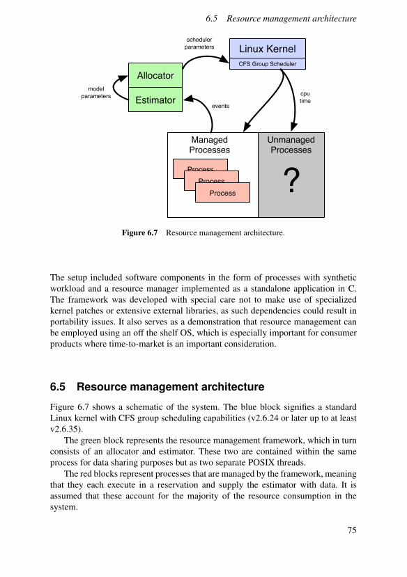
6.5 Resource management architecture
Linux Kernel
CFS Group Scheduler
Allocator
Estimator
Process
Process
Process
ManagedProcesses
UnmanagedProcesses
?
events
model
parameters
scheduler
parameters
cpu
time
Figure 6.7 Resource management architecture.
The setup included software components in the form of processes with syntheticworkload and a resource manager implemented as a standalone application in C.The framework was developed with special care not to make use of specializedkernel patches or extensive external libraries, as such dependencies could result inportability issues. It also serves as a demonstration that resource management canbe employed using an off the shelf OS, which is especially important for consumerproducts where time-to-market is an important consideration.
6.5 Resource management architecture
Figure 6.7 shows a schematic of the system. The blue block signifies a standardLinux kernel with CFS group scheduling capabilities (v2.6.24 or later up to at leastv2.6.35).
The green block represents the resource management framework, which in turnconsists of an allocator and estimator. These two are contained within the sameprocess for data sharing purposes but as two separate POSIX threads.
The red blocks represent processes that are managed by the framework, meaningthat they each execute in a reservation and supply the estimator with data. It isassumed that these account for the majority of the resource consumption in thesystem.
75

Chapter 6. Competitive resource management
MIPC - a minimalistic IPC protocolData is transmitted between components using a Minimalistic InterProcess Com-munication (MIPC) protocol developed for use with the resource manager. Data issent as datagrams and MIPC supports both local UNIX sockets and IP sockets. Asthe estimation techniques support missing measurements, the potential overhead ofusing TCP-based connections can be eliminated.
MIPC itself only handles sending raw byte data so the client will need to specifyinterfaces on top of that, typically by sharing C-struct definitions. The importantMIPC-operations are
• mipc_connect_server
• mipc_connect_client
• mipc_send
and the full API is found in Appendix A. The protocol supports the bare minimumrequired for the framework and for comparison, the compiled binary is less than 10kbytes in size and only have dependencies to the C standard library and libc, while,e.g., D-Bus, a popular interprocess communications mechanism in desktop Linuxdistributions [D-Bus 2010], is over 100 kbytes in size and has dependencies to over1 Mbytes of additional libraries.
Unmanaged processesIt is here assumed that the majority of the resource requirements comes from asubset of the running processes. The remaining is seen as noise. Should these com-ponents require a noticeable amount of resources, this will affect the estimate of therelation between the allocated share and the resulting execution rate, thus effectivelymake the CPU seem slower.
Processes or threadsKeeping a component based abstraction level is an important goal, as this gives in-creased flexibility to the software designers. By using processes to track resourceusage rather than threads, the anatomy of the components is hidden from the re-source manager. Whether a process consists of one or several threads of executionshould not matter in this framework.
Experiment setup toolsA range of Python based tools were developed in order to facilitate the scripting oftest scenarios. A Python implementation of MIPC is used to signal processes. Foroperations that require root level privileges and access to non-standard system calls,a few C-based utilities were created and then wrapped in Python code.
76

6.6 Measuring time and resource consumption
6.6 Measuring time and resource consumption
The framework requires the managed components to push data to the estimationalgorithm in the form of cycle completion events. These events contain
• a time stamp and
• a reading of the accumulated CPU-time for the component.
The resource measurement is performed as the time stamp is taken, as sending andprocessing introduce latencies. It also means that the resource cost of measuring isfactored into the overall component resource requirements, thereby distributing theoverhead rather than centralizing it on the estimator.
Measurements of resource consumption have been done using the system callclock_gettime() rather than getrusage() as it provides better precision. Analternative would to be use the cpuacct-subsystem available with control groups,but the system call was chosen as it is both simpler to use and more efficient thanparsing text files.
Reservations with CFS Group SchedulingThe group scheduling functionality (see Section 3.2) that was introduced with Linuxv2.6.24 offers an easy to use way to do soft reservations. From an experimental pointof view, this requires some extra effort as the allocation theory developed assumeshard reservations.
Shares are calculated by the algorithm as percentage of the total CPU capacity.This must then be translated into an integer number, as used by CFS, in such a waythat the desired share equals the integer weight / the sum of all weights. To avoidquantization problems, the total available shares have been selected to be 10000.The CFS scheduler does not allow for an individual reservation period to be set ona process basis so apart from share, no additional parameters must be set.
Effectuating the allocation requires writing the shares to the virtual files in acontrol group type file system.
Synthetic componentsIn order to run experiments with relevant load profiles, a synthetic component wasimplemented and instrumented with logging and a MIPC-based reconfiguration in-terface. The components execute in accordance with the cyclic component model(see Section 5.3) and with parametrized behavior. Cycle time is drawn randomlyfrom an interval specified at startup and changed periodically. The parameters thatgovern the behavior are
• k_min, k_max - controls the distribution of the cycle times.
• change_interval - determines how often cycle times are randomized.
77

Chapter 6. Competitive resource management
• rate - the rate set-point.
The components also log all completed cycles together with a snapshot of the pa-rameter set.
Estimator implementationThe estimation is a passive component in this framework and updates estimates onlywhen needed, in this case triggered by the allocation thread. A MIPC-server is setup to collect all incoming data events from the managed components, which is thenstored in a record for each individual client. The client submits a unique identifier,in this implementation the process id of the main component thread, which is thenused as a primary key in a table containing all the managed components.
The implementation supports individual estimator functions for each componentand supplies three default methods for rate estimation:
• time window (counting events over an interval)
• event window (FIR-structure, time for a fixed number of events)
• autoregressive filter of the event arrival intervals (IIR-structure)
As all events are stored, the estimation history can be replayed at the conclusion ofthe experiments and compared with the component log files.
Allocator implementationThe allocator is implemented as a periodic thread running at 1 Hz. The work orderis
• pull parameters from the estimator
• iterate the incremental solver from Section 6.2 until the potentials are withinthe tolerance level
• effectuate the allocation by writing to the cgroup file system
The allocation algorithm utilizes a red-black b-tree [Cormen, 2001] to sort the com-ponents by potential, which allows for robust performance. It is straightforward toboth add and remove tasks from the tree, thereby allowing the structure to persistbetween iterations. This circumvents the often heavy set-up portions of off-the-shelfsolvers.
A system parameter is the termination threshold. The algorithm checks thedifference in potential between the highest and lowest level and if they are closeenough, the solver terminates. In the simulations used for this thesis, the toleranceis set to 0.001.
78

6.7 Example runs
6.7 Example runs
This section presents the results from a sequence of experiments run on a desktopLinux computer. The hardware was a 2.4 Ghz Pentium 4 with 512 Mb of main mem-ory running a Linux 2.6.27-based Debian system. The background noise consistsof the software that runs on a typical Debian desktop, including the X11/Gnomegraphical environment, as well as an Apache web server and a MySQL databaseengine.
Estimation and controlThe first experiment is to validate the estimation and control strategy. A single soft-ware component with constant but unknown cycle execution time is here controlledusing feedforward based on an estimation of the k-parameter.
Figures 6.8 and 6.9 show the scenario using one second time window estima-tion and a 15 long event window estimation respectively. The time window per-forms well at higher rates, having more information to form the estimate, while theevent window estimator is more responsive to change. The AR-approach proved tobe difficult to tune, resulting in much noisier estimates, and was not used for theexperiments.
Constrained allocationIn this scenario, three components are running in a situation where the system isoverloaded. The components change their cycle execution rates randomly every 3seconds, with k_max/k_min equal to 2. Figure 6.10 shows the estimated rates overtime and Figure 6.11 displays the cost for the dynamic convex allocation (DCA)with a comparison with static worst case allocation (SWA), i.e., the performanceattained by only allocating resources based on the worst case execution time. To-wards the end of the experiment, the component set is close to their worst case cycletimes, and this causes the system cost to approach that of the worst case allocation.
To study how the performance depends on the level of uncertainty, a series ofexperiments were run with increasing k_max/k_min. In scenarios with low uncer-tainty, the dynamic strategy performs worse than the static alternative, as the esti-mated parameters will, due to the presence of noise, never be completely correct.However, as uncertainty grows, the dynamic strategy shows significant performanceadvantages, which is shown in Figure 6.12.
6.8 Conclusions
This chapter has introduced a method for dynamic resource allocation based onconvex programming and a rate based utility model for cyclic software components.An algorithm designed to efficiently solve the resulting optimization problem on
79

Chapter 6. Competitive resource management
0 2 4 6 8 10 12 14time (s)
10
20
30
40
50
60
70
rate
(events
/s)
Estimated rate using sliding time window (1s)
estimated ratebw / set point
Figure 6.8 Estimation and control using time window
0 2 4 6 8 10 12 14time (s)
10
20
30
40
50
60
70
rate
(events
/s)
Estimated rate using FIR-estimator (m=15)
estimated ratebw / set point
Figure 6.9 Estimation and control using event window
80

6.8 Conclusions
0 2 4 6 8 10 12 14time (s)
0
5
10
15
20
25
30
rate
(events
/ s
)
112631126711264
Figure 6.10 Allocation in an over-utilized system with rates estimated using a onesecond time window.
0 2 4 6 8 10 12 14 16time (s)
2000
3000
4000
5000
6000
7000
8000
Cost
J
DCASWA
Figure 6.11 Cost for Dynamic Convex Allocation (DCA) vs Static Worst case Al-location (SWA) over time.
81

Chapter 6. Competitive resource management
1 2 3 4 5 6 7 8 9k_max / k_min
0
5000
10000
15000
20000
25000norm
(J)
SWADCA
Figure 6.12 Average Cost for Dynamic Convex Allocation (DCA) vs Static Worstcase Allocation (SWA) as uncertainty grows.
limited precision hardware has been presented together with analysis of its runtimeperformance.
Results from experiments run on an implementation of the resource manage-ment scheme on Linux has are presented with comparisons to the correspondingworst case-based performance.
82

7Collaborative resourcemanagement
This chapter discusses the application of feedback control to a system where com-ponent are dependent on each other. More specifically, the results presented herepertains to systems where the performance metrics are functions of how the compo-nents collaborate around tasks, hence the term collaborative resource management.As a result, the theory presented does not build on Chapter 6, and instead presents analternative scenario where adding resources to a component may even reduce sys-tem performance. The component model used is, however, still based on Chapter 5.The thermal control approach is further validated by an implementation on a mobilerobot. The chapter is based on [Lindberg and Årzén, 2010b; Romero Segovia et al.,2011].
7.1 Allocation vs feedback
One of the key simplifications made in the resource allocation algorithm proposedin Chapter 6 was to optimize the performance in a stationary sense, as introducingstate dynamics into the optimization would require a more comprehensive solver. Assuch, the allocation strategy used in this thesis is largely a feedforward solution andtherefore blind to performance metrics explicitly connected to state information.
Given perfect information about execution times and resource availability, thesemetrics could be controlled through the allocation strategy. However, as a centraltheme of this work is the presence of uncertainty and disturbances, it must be as-sumed that this is not possible. Specifically, it can be expected that transient phe-nomena will occur due to disturbances and structural changes in the system, such ashardware interrupts and the activation or reconfiguration of components. Assumingthat these occurrences cannot be predicted, they must be addressed through feed-back.
83

Chapter 7. Collaborative resource management
C1 C2
q(t)
Figure 7.1 Two components connected through a FIFO-queue. q(t) signifies thenumber of elements in the queue.
7.2 State related performance metrics
The two aspects of performance that will be discussed here are
• integrator dynamics and
• state transition events.
Queues and integratorsAsynchronous communication between components in software systems is com-monly done through FIFO-queues. This is practiced both in consumer grade mul-timedia frameworks such as GStreamer [Taymans et al., 2010] and more academi-cally oriented actor-based languages such as CAL [Bhattacharyya et al., 2009; Ekerand Janneck, 2003]. A common problem that arises in such designs is the regulationof queue sizes, as this affects both end-to-end computational latency and storage re-quirements.
If a queue constitutes the connection from component C1 to C2, as illustratedin Figure 7.1, and q(t) denotes the number of queue entries at time t, its resourcedependent dynamics could be described by
y1(t) = k1u1(t)
y2(t) = k2u2(t)
q(t +h) = q(t)+h(y1(t)− y2(t))(7.1)
i.e., a discrete time integrator. From an allocation point of view, an imbalance be-tween y1 and y2 results in either starvation of C2 or unbounded queue length. There-fore, the feedforward strategy should strive for y1 = y2. Transient effects can thenbe attenuated through feedback.
State transitionsState models are commonly used for software systems, defining the behavior interms of states and state transitions. A state transition is caused by some internal orexternal dynamic and the passing from one state to another represents an event thatis significant to the software. This could for instance be the completion of a com-putation, e.g., the decoding of a video frame or the termination of an optimization.
84
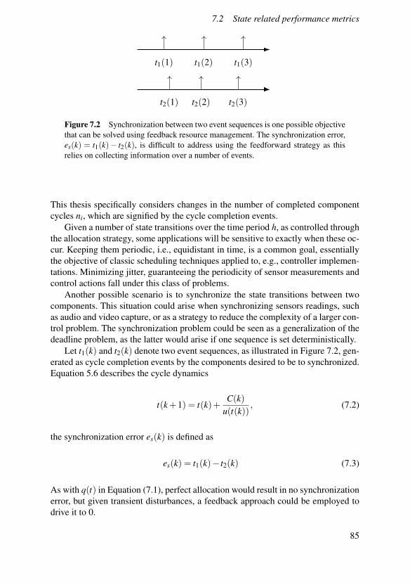
7.2 State related performance metrics
t1(1) t1(2) t1(3)
t2(1) t2(2) t2(3)
Figure 7.2 Synchronization between two event sequences is one possible objectivethat can be solved using feedback resource management. The synchronization error,es(k) = t1(k)− t2(k), is difficult to address using the feedforward strategy as thisrelies on collecting information over a number of events.
This thesis specifically considers changes in the number of completed componentcycles ni, which are signified by the cycle completion events.
Given a number of state transitions over the time period h, as controlled throughthe allocation strategy, some applications will be sensitive to exactly when these oc-cur. Keeping them periodic, i.e., equidistant in time, is a common goal, essentiallythe objective of classic scheduling techniques applied to, e.g., controller implemen-tations. Minimizing jitter, guaranteeing the periodicity of sensor measurements andcontrol actions fall under this class of problems.
Another possible scenario is to synchronize the state transitions between twocomponents. This situation could arise when synchronizing sensors readings, suchas audio and video capture, or as a strategy to reduce the complexity of a larger con-trol problem. The synchronization problem could be seen as a generalization of thedeadline problem, as the latter would arise if one sequence is set deterministically.
Let t1(k) and t2(k) denote two event sequences, as illustrated in Figure 7.2, gen-erated as cycle completion events by the components desired to be to synchronized.Equation 5.6 describes the cycle dynamics
t(k+1) = t(k)+C(k)
u(t(k)), (7.2)
the synchronization error es(k) is defined as
es(k) = t1(k)− t2(k) (7.3)
As with q(t) in Equation (7.1), perfect allocation would result in no synchronizationerror, but given transient disturbances, a feedback approach could be employed todrive it to 0.
85

Chapter 7. Collaborative resource management
7.3 Hardware resources
Availability of the CPU resource is limited by hardware performance. Power andheat are two types of constraints in this setting. In this thesis the problem of thermalmanagement is considered.
Normally a CPU can only operate properly if the temperature is kept belowa certain level but if there is no active cooling, as is the case in many embeddedplatforms, this must be respected through control of CPU power. The options todo this include voltage- and frequency scaling and idling (e.g., executing the HLTinstruction [Intel, 2010]), the last of which will be used here. The main reason forthis is that the speed of the CPU directly affects the component model parametersand any on-line estimates would then change due to control action. Controlling thetemperature through the resource level U and then imposing the limit
N
∑i=1
ui ≤U (7.4)
simplifies the estimation strategy. Control can be effectuated through limiting theavailable CPU-time using an RBS framework. The resource level U is then de-termined by the thermal control algorithm, which becomes a part of the resourcecontroller.
Thermal controlGiven that the temperature is modeled with first order dynamics with slow distur-bances, a PI-controller [Åström and Murray, 2008] is a simple and effective choice,though anti-windup measures must be added to handle effects from control signalsaturation.
The pure PI-controller is defined as
u(t) = K(e(t)+1Ti
∫ t
0e(τ)dτ) (7.5)
By discretization of the dynamics using a forward Euler approximation, constrain-ing the control signal U to the interval [0,1] and adding an anti-windup trackingterm to the integral part, the resulting control algorithm, described as pseudo-code,is
e := r - y_T;V := K*e + I;U := sat(V, 0, 1);if (Ti > 0) then
I := I + K*h*e/Ti + K*h/Tr*(U - V);else
I := 0;endif
86

7.4 Case study — Encoding Pipeline
CPUResourceController
AudioEncoder
VideoEncoder
QA
QV
NetworkStack
T
cputime
U
ua
un
uv
ya
yv
yn
Figure 7.3 An overview of the conversational video pipeline
where h is the sampling interval, K,Ti are the PI-controller parameters and Tr is theanti-windup tracking gain.
7.4 Case study — Encoding Pipeline
The prototypical system to be considered is a conversational video pipeline as dis-played in Figure 7.3. The software part consists of three tasks, an audio encoder, avideo encoder and a network stack. The encoders are assumed to have private accessto capturing hardware and it is also assumed that they are capable of variable rateexecution. The encoders are connected to the network through the FIFO-queues QAand QV. In order to send a network packet, the stack requires one frame of audioand video.
In order to evaluate the performance of this system, the following metrics aredefined
• Sync error. It is disturbing to the human eye when video and audio are out ofsync and therefore it is natural to consider the difference in encoding times-tamp between the corresponding audio and video frames. If both tasks areassumed to be cyclic and ta(k) and tv(k) denote the encoding timestamps foraudio and video frames respectively, then
ta(k+1) = ta(k)+Ca(k)
ua(t(k))
tv(k+1) = tv(k)+Cv(k)
uv(t(k))
(7.6)
would be the corresponding dynamics. The sync error es(k) is then defined as
es(k) = ta(k)− tv(k) (7.7)
• Latency. Delay in the conversation is also an important quality metric andfor this set up this will be the end to end latency, i.e., the delay from capture
87

Chapter 7. Collaborative resource management
to network. If qa(t) and qv(t) are the number of elements at time t in QA andQV respectively, then let the average encoding latency el(t) be defined as thesum of the encoding delay Da,v and the network delay Dn.
The encoding delay is modeled as
Da,v =
Ca(k)ua(ta(k))
+Cv(k)
uv(tv(k))2
(7.8)
which is the the average of the audio encoding time and video decoding timeand the network delay as
Dn = (qa(t)+qv(t)
2+1)
Cn(k)un(tn(k))
(7.9)
i.e., the time it takes to process the queue backlog plus one cycle time for thepacket itself. el(t) is then defined as
el(t) = Da,v +Dn (7.10)
or in words, the computational delay combined with the network backlog inthe queues.
• Queue dynamics. Using the cycle dynamics expressed in Equation (7.1), thedynamics of qa and qv is modeled as
qa(t +h) = qa(t)+h(ya− yn)
qv(t +h) = qv(t)+h(yv− yn)(7.11)
Control designLatency It follows from (7.10) and (5.7) that latency can be controlled throughminimizing the queue lengths and then keeping a uniform steady state cycle timeacross all components. The approach taken in this work is to combine feedforwardcontrol based on the total amount of resource with feedback re-allocation to reducequeue length.
The nominal feedforward controls are computed by combining the constraintthat ua +uv +un ≤U from Equation (7.4) with
ya = yv = yn = y, (7.12)
i.e., a steady state where the execution rates ya, yv and yn are the same. From this itfollows that
1ka
+1kv
+1kn
=Uy
(7.13)
88
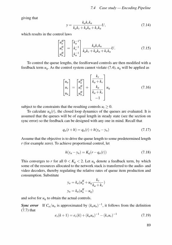
7.4 Case study — Encoding Pipeline
giving that
y =kakvkn
kakv + kakn + kvknU, (7.14)
which results in the control lawsuffa
uffv
uffn
=
k−1a
k−1v
k−1n
kakvkn
kakv + kakn + kvknU. (7.15)
To control the queue lengths, the feedforward controls are then modified with afeedback term uq. As the control system cannot violate (7.4), uq will be applied as
ua
uv
un
=
uffa
uffv
uffn
+
kv
ka + kv
ka
ka + kv
−1
uq (7.16)
subject to the constraints that the resulting controls ui ≥ 0.To calculate uq(t), the closed loop dynamics of the queues are evaluated. It is
assumed that the queues will be of equal length in steady state (see the section onsync error) so the feedback can be designed with any one in mind. Recall that
qa(t +h) = qa(t)+h(ya− yn) (7.17)
Assume that the objective is to drive the queue length to some predetermined lengthr (for example zero). To achieve proportional control, let
h(ya− yn) = Kq(r−qa(t)) (7.18)
This converges to r for all 0 < Kq < 2. Let uq denote a feedback term, by whichsome of the resources allocated to the network stack is transferred to the audio- andvideo decoders, thereby regulating the relative rates of queue item production andconsumption. Substitute
ya = ka(uffa +uq
kv
ka + kv)
yn = kn(uffn −uq)
and solve for uq to obtain the actual controls.
Sync error If Ca/ua is approximated by (kaua)−1, it follows from the definition
(7.7) thates(k+1) = es(k)+(kaua)
−1− (kvuv)−1 (7.19)
89

Chapter 7. Collaborative resource management
ThermalControl
Estimator
QueueControl
FlowControl
SyncControl
+ +yT
ni
qi
es
ResourceController
U
ki
uff
biuq
us
ui
Figure 7.4 The resulting control structure including estimation, feedforward flowcontrol based on the estimated model parameters and the available CPU resource andfeedback based on queue state and sync error. bi refers to the coefficients in Equation(7.16).
As there is a finite combined flow of CPU resource to the audio and video encoder,the approach taken here is to introduce us as a feedback term, modifying the feed-forward allocation so that
es(k+1) = es(k)+(ka(ua +us))−1− (kv(uv−us))
−1 (7.20)
is driven towards zero. While this seems to interfere with the queue control, the dif-ference in time scale between the event-to-event dynamics makes its effects on theslower queue controller negligible. In fact, it is seen in Section 7.5 that controllingthe sync error actually greatly simplifies the queue control. For proportional control,let
(ka(ua +us))−1− (kv(uv−us))
−1 = Kses(k) (7.21)
Under deterministic circumstances the sequence es(k) will converge to zero for anyKs ∈ (0,−2). Given the variations in the cycle execution times, some care should betaken when selecting Ks so that noise is not unnecessarily amplified. As this workis done without a detailed noise model, Ks is chosen conservatively as -0.5. Theresulting equation is then solved under the constraint that ua+us≥ 0 and uv−us≥ 0to obtain us.
The resulting control structure is presented in Figure 7.4.
90

7.5 Simulation results
0 20 40 60 80 100k
0.010
0.015
0.020
0.025
0.030
0.035
0.040
0.045
0.050Ci(k)
AudioEncoder VideoEncoder NetworkStack
Figure 7.5 Generated cycle times used in the simulation examples below.
7.5 Simulation results
Simulation environmentIn order to evaluate controls, a simulation environment has been developed inPython. The system dynamics is approximated by discretization with a time stepof 1 ms, which incurs quantization on the cycle completion time stamps. This is,however, assumed to be of little effect as the variation due to noise is orders ofmagnitude greater for these simulations.
Cycle execution times have been generated as Di +Xi(k) where Di is an a-prioriunknown constant and Xi(k) ∈ exp(0.1Di). The realizations used for the presentedsimulation results are shown in Figure 7.5. The randomness is meant to model bothsoftware execution time uncertainty and the stochastic properties of a modern CPU,including the effects of caches, the memory bandwidth gap and deep pipelines.The Di values were chosen randomly so that the resulting k-parameters would liebetween 10 and 100. A real sequence of cycle times for a video decoder is providedfor comparison in Figure 7.6. h is globally defined as 1.
91

Chapter 7. Collaborative resource management
0 20 40 60 80 100 120k
0.0015
0.0020
0.0025
0.0030
0.0035
0.0040
0.0045C
(k)
MPEG-2 decoder sequence
Figure 7.6 A sequence of execution times for an MPEG-2 decoder working on avideo stream. This encoding standard interleaves complete image descriptions withdelta descriptions. Decoding a complete image is significantly harder, causing thehigh peaks.
Thermal controlThe thermal model of the CPU is based on [Fu et al., 2010b], but to make the effectsof the thermal dynamics more visible in the simulations, the parameters have beenscaled so the dynamics are faster. This makes the effects of control and disturbancesmore prominent. In the simulations, the parameters in Equation (5.8) are chosen asa = 2 and b = 1.5. The main purposes of the thermal model are
• to provide a scenario for the varying availability of CPU resource and
• to show how physical models can be combined with the software models,
so switching for more realistic parameters would not change the design decisionssignificantly though the thermal controller must then be re-tuned. However, as thefocus of this thesis is on the application performance as affected by both hardwareand software, more advanced temperature control strategies are left for future re-search.
92

7.5 Simulation results
0 2 4 6 8time(s)
55
60
65
70
75
80
85
T (
degre
e C
)
T controlledT UncontrolledT ref
0 2 4 6 8time(s)
�0.5
0.0
0.5
1.0
1.5
2.0
U
U=sat(P+I,0,1)P-partI-part
Figure 7.7 PI control of temperature with a constant disturbance of 15 degrees C /s entering at 5s. The uncontrolled dynamics are shown for comparison.
A scenario where a disturbance enters occurs at 5 seconds is shown in Figure7.7. This could be a situation where the unit is left in direct sunlight that causes aninsolation effect of 15 degrees C / s. The controller keeps the temperature by throt-tling the available CPU-time. As the temperature approaches the set point, the totalutilization is lowered to about 80%. At 5 seconds, the disturbance causes the tem-perature to rise and the controller responds by lowering the utilization even further,settling at about 55%. If there are no active cooling measures or direct measure-ments of external disturbances, the set point must be sufficiently below the criticallevel to keep the CPU from overheating.
Parameter estimationFigure 7.8 shows the estimated execution rates and corresponding ki-parameter es-timates over the same simulation. The discontinuous nature of the virtual flows isevident in these plots. Note that it takes some time before the network stack startsto execute and this is because of the queue-controller. It throttles the network stackwhile the queues are filled and because of this, the k-parameter estimator needsmore time to form kn. This causes the large overshoot in the queue length before itsettles on the desired level.
93

Chapter 7. Collaborative resource management
0 2 4 6 8time(s)
0
20
40
60
80
100
120
140
k
AudioEncoder VideoEncoder NetworkStack
0 2 4 6 8time(s)
0
5
10
15
20
25
30
yAudioEncoder VideoEncoder NetworkStack
Figure 7.8 Rate and parameter estimation for all three tasks. Rates are estimatedby counting events with a sliding time window with length 1 second. The networkstack (red) lags behind in the beginning due to queue control.
Even though the actual execution rate changes over time, the estimate meanremains stable while the variance increases as the execution rates drop in the laterpart of the simulation, as seen in the upper plot. This is because a single event beingoutside or inside the estimation window will affect the estimate more. The window-based estimation scheme will break down when the rate drops below 1 cycle persecond.
Latency performanceAs there is no information about future demands for the CPU resource, a reasonablestrategy is to minimize latency at all times. This is done by utilizing all availableCPU-time while respecting the temperature set-point, thereby reducing the execu-tion time for all tasks, and by controlling the queues. The reason why the queuecontroller is not trying to drive the queue lengths to zero is that this could causeblocking in the network stack, which in turn would reduce the accuracy of kn. Thiscould be treated by designing a better estimator.
The latency control performance is displayed in Figure 7.9. A scenario withoutqueue control is provided for comparison and the problem with this is evident. Even
94
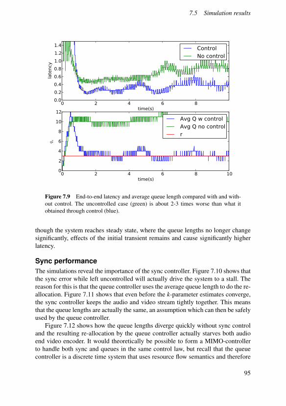
7.5 Simulation results
0 2 4 6 8time(s)
0.0
0.2
0.4
0.6
0.8
1.0
1.2
1.4la
tency
ControlNo control
0 2 4 6 8 10time(s)
0
2
4
6
8
10
12
q v
Avg Q w controlAvg Q no controlr
Figure 7.9 End-to-end latency and average queue length compared with and with-out control. The uncontrolled case (green) is about 2-3 times worse than what itobtained through control (blue).
though the system reaches steady state, where the queue lengths no longer changesignificantly, effects of the initial transient remains and cause significantly higherlatency.
Sync performanceThe simulations reveal the importance of the sync controller. Figure 7.10 shows thatthe sync error while left uncontrolled will actually drive the system to a stall. Thereason for this is that the queue controller uses the average queue length to do the re-allocation. Figure 7.11 shows that even before the k-parameter estimates converge,the sync controller keeps the audio and video stream tightly together. This meansthat the queue lengths are actually the same, an assumption which can then be safelyused by the queue controller.
Figure 7.12 shows how the queue lengths diverge quickly without sync controland the resulting re-allocation by the queue controller actually starves both audioend video encoder. It would theoretically be possible to form a MIMO-controllerto handle both sync and queues in the same control law, but recall that the queuecontroller is a discrete time system that uses resource flow semantics and therefore
95
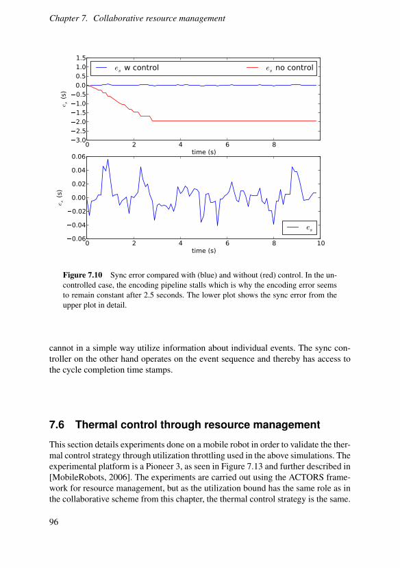
Chapter 7. Collaborative resource management
0 2 4 6 8time (s)
�3.0
�2.5
�2.0
�1.5�1.0�0.5
0.0
0.5
1.0
1.5e s
(s)
es w control es no control
0 2 4 6 8 10time (s)
�0.06
�0.04
�0.02
0.00
0.02
0.04
0.06
e s (
s)
es
Figure 7.10 Sync error compared with (blue) and without (red) control. In the un-controlled case, the encoding pipeline stalls which is why the encoding error seemsto remain constant after 2.5 seconds. The lower plot shows the sync error from theupper plot in detail.
cannot in a simple way utilize information about individual events. The sync con-troller on the other hand operates on the event sequence and thereby has access tothe cycle completion time stamps.
7.6 Thermal control through resource management
This section details experiments done on a mobile robot in order to validate the ther-mal control strategy through utilization throttling used in the above simulations. Theexperimental platform is a Pioneer 3, as seen in Figure 7.13 and further described in[MobileRobots, 2006]. The experiments are carried out using the ACTORS frame-work for resource management, but as the utilization bound has the same role as inthe collaborative scheme from this chapter, the thermal control strategy is the same.
96

7.6 Thermal control through resource management
0 1 2 3 4 5time(s)
0
5
10
15
20
25
30
yAudioEncoder VideoEncoder NetworkStack
0 1 2 3 4 5time(s)
�5
0
5
10
15
20
25
30
y
AudioEncoder VideoEncoder NetworkStack
Figure 7.11 Execution rates compared with and without sync control. The curveshave been averaged over a window of 0.1 s to provide better visibility.
System modelIn order to prevent CPU processor overheating, which could cause performancedegradation of all the applications executing on the system and even system fail-ure, a system model that combines feedback and feedforward techniques to controlboth the temperature and the utilization of the processor (CPU) through adaptivebandwidth allocation is proposed. Figure 7.14 shows the proposed system model,which combines the features of a thermal controller, that keeps the temperature ofthe system bounded to a desirable temperature acceptable to the processor, and aresource manager that dynamically allocates resources to each application on thesystem. Here, T and TR are the current temperature of the system, and the refer-ence temperature respectively, it is assumed that this last value can be specified bythe user. The values U , Umin, Umax and UL correspond to the utilization of the sys-tem, the lower and upper utilization bounds and the utilization limit defined by thethermal controller respectively.
97

Chapter 7. Collaborative resource management
0 2 4 6 8time (s)
�5
0
5
10
15
20
25
q a, q v
qa
qv
0 2 4 6 8time(s)
�0.2
0.0
0.2
0.4
0.6
0.8
1.0
1.2
ui
AudioEncoder VideoEncoder NetworkStack
Figure 7.12 Queue lengths for a scenario with no sync control. The resulting allo-cation is based on the average queue length (qa +qv)/2.
Software componentsDue to system limitations, as well as performance specifications, it is convenientto keep the temperature of the system bounded to a desired value. From a softwarepoint of view, this can be achieved using bandwidth reservation techniques [Abeniand Buttazzo, 1998a], which in combination with control theory allow at runtimeadaptive allocation of CPU resources provided to the applications. Reservation tech-niques such as the constant-bandwidth server (CBS), guarantee to each applicationa certain execution budget every server period, this is also known as virtual pro-cessors (VP). In order to achieve this adaptive allocation of resources, a modifiedversion of the architecture proposed originally by ACTORS (see e.g. [Segovia andÅrzén, 2010]) is used, which assumes a multicore physical platform. For this par-ticular case, a single core physical platform was employed. Figure 7.15 shows themodified architecture, which is composed mainly of three components: the applica-tions, the resource manager (RM) and the reservation layer which includes the VPsof each application.
The RM is a daemon application, composed of a centralized supervisor andseveral bandwidth controllers, these elements will be explained in Section 7.7. The
98
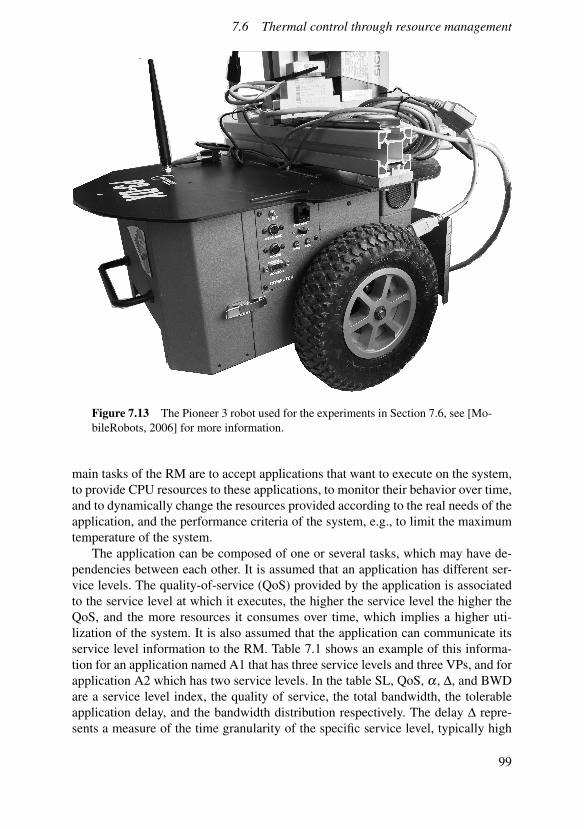
7.6 Thermal control through resource management
Figure 7.13 The Pioneer 3 robot used for the experiments in Section 7.6, see [Mo-bileRobots, 2006] for more information.
main tasks of the RM are to accept applications that want to execute on the system,to provide CPU resources to these applications, to monitor their behavior over time,and to dynamically change the resources provided according to the real needs of theapplication, and the performance criteria of the system, e.g., to limit the maximumtemperature of the system.
The application can be composed of one or several tasks, which may have de-pendencies between each other. It is assumed that an application has different ser-vice levels. The quality-of-service (QoS) provided by the application is associatedto the service level at which it executes, the higher the service level the higher theQoS, and the more resources it consumes over time, which implies a higher uti-lization of the system. It is also assumed that the application can communicate itsservice level information to the RM. Table 7.1 shows an example of this informa-tion for an application named A1 that has three service levels and three VPs, and forapplication A2 which has two service levels. In the table SL, QoS, α , ∆, and BWDare a service level index, the quality of service, the total bandwidth, the tolerableapplication delay, and the bandwidth distribution respectively. The delay ∆ repre-sents a measure of the time granularity of the specific service level, typically high
99

Chapter 7. Collaborative resource management
Figure 7.14 System model
Figure 7.15 Modified ACTORS architecture
QoS levels have a low value of ∆. The bandwidth distribution is an optional value, itis an indication from the application to the RM how this total bandwidth should bedistributed over the individual virtual processors. Additionally the RM is informedabout the total number of VPs that each application contains and the importance ofthe application relative to others.
The information provided by the application (see Table 7.1) represents an ini-tial estimate of the resources required at an specific service level. This informationconstitutes an initial model of the application, which during run-time and throughthe control mechanism implemented by the RM will be tuned appropriately.
100

7.7 Control design
Table 7.1 Service level table for application A1 and A2
Application SL QoS α ∆ BWDname [%] [%] [µs] [%]A1 0 100 100 28-24-24 40-30-30
1 80 70 42-48-48 30-20-202 60 40 80-90-90 20-10-10
A2 0 100 60 201 80 40 50
7.7 Control design
The proposed thermal control algorithm together with the resource manager aredesigned to meet two fundamental requirements: to prevent processor overheatingby minimizing the maximum temperature of the system, and to provide desiredsystem performance by maximizing the QoS provided by the running applicationssubject to the resource limitations.
Thermal control designTo fulfill the first objective of our control design, the use of a PI algorithm forthe thermal controller is proposed. As shown in Figure 7.16, the signal T from
Figure 7.16 Thermal controller structure
the temperature sensor is passed through a FIR filter, which reduces measurementnoise. The filtered temperature TF is then compared with the reference temperatureTR, producing the error input of the PI controller. Additionally to this input thecontroller uses the utilization signal U provided by the resource manager, whichrepresents the current CPU load caused by the applications running at an specificservice level on the system. This signal is used by the anti-windup component ofthe PI controller to prevent wind up of the integral part.
The additional inputs Umin and Umax, represent the minimum utilization requiredby the applications to provide an specific QoS, and the maximal permissible utiliza-tion defined by the employed scheduling policy respectively. These two inputs pro-vide the lower and upper limits that bound the PI controller output u(k) such that,
101
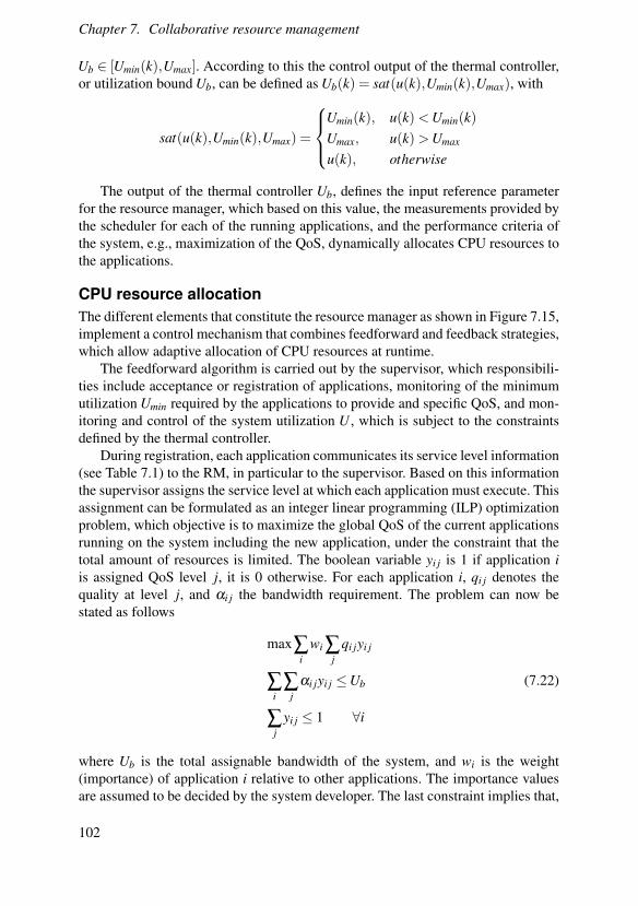
Chapter 7. Collaborative resource management
Ub ∈ [Umin(k),Umax]. According to this the control output of the thermal controller,or utilization bound Ub, can be defined as Ub(k) = sat(u(k),Umin(k),Umax), with
sat(u(k),Umin(k),Umax) =
Umin(k), u(k)<Umin(k)Umax, u(k)>Umax
u(k), otherwise
The output of the thermal controller Ub, defines the input reference parameterfor the resource manager, which based on this value, the measurements provided bythe scheduler for each of the running applications, and the performance criteria ofthe system, e.g., maximization of the QoS, dynamically allocates CPU resources tothe applications.
CPU resource allocationThe different elements that constitute the resource manager as shown in Figure 7.15,implement a control mechanism that combines feedforward and feedback strategies,which allow adaptive allocation of CPU resources at runtime.
The feedforward algorithm is carried out by the supervisor, which responsibili-ties include acceptance or registration of applications, monitoring of the minimumutilization Umin required by the applications to provide and specific QoS, and mon-itoring and control of the system utilization U , which is subject to the constraintsdefined by the thermal controller.
During registration, each application communicates its service level information(see Table 7.1) to the RM, in particular to the supervisor. Based on this informationthe supervisor assigns the service level at which each application must execute. Thisassignment can be formulated as an integer linear programming (ILP) optimizationproblem, which objective is to maximize the global QoS of the current applicationsrunning on the system including the new application, under the constraint that thetotal amount of resources is limited. The boolean variable yi j is 1 if application iis assigned QoS level j, it is 0 otherwise. For each application i, qi j denotes thequality at level j, and αi j the bandwidth requirement. The problem can now bestated as follows
max∑i
wi ∑j
qi jyi j
∑i
∑j
αi jyi j ≤Ub (7.22)
∑j
yi j ≤ 1 ∀i
where Ub is the total assignable bandwidth of the system, and wi is the weight(importance) of application i relative to other applications. The importance valuesare assumed to be decided by the system developer. The last constraint implies that,
102

7.7 Control design
if necessary, some low important applications might be turned off, in order to allowthe registration of more important applications.
After the service level assignment of each application, the supervisor calculatesthe reservation parameters of each VP. Hence, it creates the VPs for the tasks of eachapplication by defining the budget Q, and the period P of each VP. The calculationof the budget and the period of the server is based on the corresponding (α,∆) (see[Mok et al., 2001a]) parameters described by the following equation
Q = αP P =∆
2+Q (7.23)
The service level assignment of the applications running on the system, is car-ried out not only during registration, but also when the thermal controller redefinesthe utilization limit Ub. This could be the result of abrupt temperature increments inthe system caused by internal factors, such as a high computational load of the run-ning applications, or by external ones such as overheated adjacent equipment. Anyof these situations would trigger a new service level assignment for all applications.
The service level assigned to each application running on the system, sets aninitial upper limit for the assigned budget also known as ABL, this value can bedirectly calculated from the information provided by the application (see Table 7.1).
The feedback mechanism is implemented by the bandwidth controllers of theVPs of each application. They check, whether or not the tasks within the VPs makeoptimal use of the bandwidth provided, or the assigned budget (AB), and take ac-tions to ensure this without degrading the performance of the application. The band-width controllers are executed periodically with a period that is a multiple of theperiod of the VP that they are controlling.
The bandwidth controllers measure the actual resource consumption using twomeasurements provided by the scheduler. The used budget (UB) is the average usedbudget over the sampling period of the controller at the current assigned servicelevel. Considering that the linux scheduler SCHED_EDF, the name used by an earlyversion of SCHED_DEADLINE, supports hard reservations, the UB is always lessthan or equal to the budget that has been assigned to the VP by the RM. The hardreservation (HR) is a value that tells the percentage of server periods over the lastsampling period that the task in the VP consumed its full budget. This is an indicatorof the number of deadlines missed.
The bandwidth controllers have a cascade structure shown in Figure 7.17. TheHRSP corresponds to the maximum percentage of deadlines misses that can be al-lowed in each sampling period. The controller C1 defines the new value of the UBSP,which in this case corresponds to the upper and lower bounds within which the UBshould reside. In the case the bounds are violated, the controller C2 either increasesor decreases the assigned budget AB of the VP, this subject to the imitation de-fined by the supervisor. The value of HRSP can be related to the performance of theapplication.
103

Chapter 7. Collaborative resource management
Figure 7.17 Resource manager controller structure
7.8 Implementation
The thermal control algorithm has been implemented together with the modifiedACTORS framework. The implementation was done on a Pioneer mobile robot[MobileRobots, 2006] with an internal Intel Pentium III based computer [ModelVSBC-8 Reference manual 2007]. The thermal sensor used is a National Semicon-ductor LM83 chip with an accuracy of±3◦C [National Semiconductor Corporation,1999], and sample period of 2 seconds. The D/A-conversion takes approximately500 ms and the temperature measurement is updated by the sensor driver every twoseconds [Delvare, 2010]. In order to avoid aliasing effects, the sampling period ofthe bandwidth controllers is set to a multiple of the application granularity that ishigher than the D/A conversion time.
A PI controller, designed as discussed in Section 7.7 is used to calculate the uti-lization limit parameter, that keeps the temperature of the system around a referencevalue provided by the user. To limit the measurement noise, the temperature signalis passed through a FIR filter with a rectangular window of one minute. The thermalcontroller is set to run as often as new data is available from the sensor, i.e., everytwo seconds, this is done to get as much data as possible to improve the filtering.The utilization bound Ub calculated by the controller defines one of the constraintsof the service level assignment problem defined by equation 7.22. In order to solvethe ILP optimization problem, the RM uses the GLPK linear programming toolkit[Makhorin, 2000].
The reservation mechanism is provided by the Linux scheduling classSCHED_EDF. The measured system utilization value only considers the applica-tions that register with the resource manager, and not the RM itself which has afixed amount of resources allocated by the system. For this implementation themaximum utilization Umax was set to 80%. Every time that the utilization limit
104
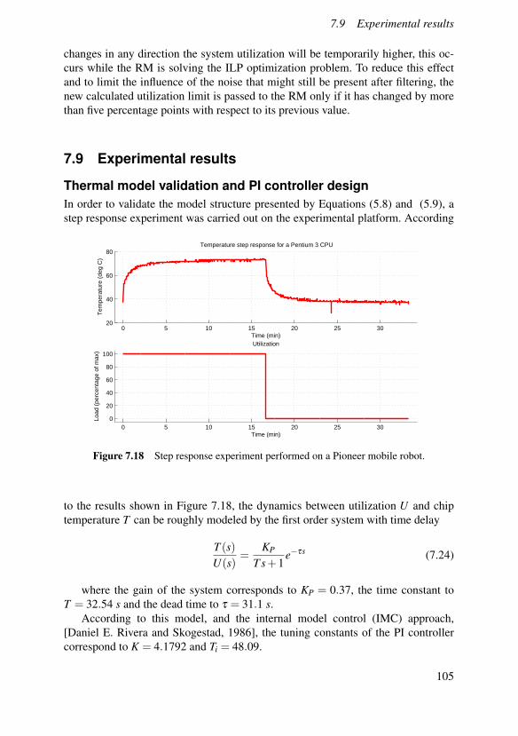
7.9 Experimental results
changes in any direction the system utilization will be temporarily higher, this oc-curs while the RM is solving the ILP optimization problem. To reduce this effectand to limit the influence of the noise that might still be present after filtering, thenew calculated utilization limit is passed to the RM only if it has changed by morethan five percentage points with respect to its previous value.
7.9 Experimental results
Thermal model validation and PI controller designIn order to validate the model structure presented by Equations (5.8) and (5.9), astep response experiment was carried out on the experimental platform. According
0 5 10 15 20 25 3020
40
60
80Temperature step response for a Pentium 3 CPU
Time (min)
Tem
pera
ture
(de
g C
)
0 5 10 15 20 25 300
20
40
60
80
100
Utilization
Time (min)
Load
(pe
rcen
tage
of m
ax)
Figure 7.18 Step response experiment performed on a Pioneer mobile robot.
to the results shown in Figure 7.18, the dynamics between utilization U and chiptemperature T can be roughly modeled by the first order system with time delay
T (s)U(s)
=KP
T s+1e−τs (7.24)
where the gain of the system corresponds to KP = 0.37, the time constant toT = 32.54 s and the dead time to τ = 31.1 s.
According to this model, and the internal model control (IMC) approach,[Daniel E. Rivera and Skogestad, 1986], the tuning constants of the PI controllercorrespond to K = 4.1792 and Ti = 48.09.
105

Chapter 7. Collaborative resource management
Experimental setupIn order to see the performance of the proposed algorithm under normal and over-loaded conditions, two different experiments were carried out. In the first experi-ment the reference temperature was set to 55◦C for a period of 10 minutes, and thenchanged to 45◦C for another 10 minutes. For the second experiment the referencetemperature was kept constant at 50◦C.
Since the objective of these experiments is to show the performance of the ther-mal controller working together with the resource manager, the service level tablesof applications A1 and A2 are defined such that, the ILP optimization problem de-fined by Equation 7.22 always finds a feasible solution. The infeasible solution casewhich is handled by a bandwidth compression algorithm, and the tuning of the val-ues on the service level tables are outside the scope of this thesis.
For the first experiment, a pipeline application A1 consisting of two tasks T 11
and T 12 with random execution times was used. As described in Section 7.7, during
registration the application provides its service level information (see Table 7.2) tothe RM. Since there are enough resources in the system, the RM assigns servicelevel 0 to A1.
The first plot in Figure 7.19 shows the behavior of the filtered system tempera-ture (green) with respect to the reference temperature (red). The second plot displaysthe measured utilization (green) and the utilization limit (red), which is the output ofthe thermal controller. The third plot shows the service levels of the application A1.The changes are done to compensate for the reference temperature change. The lastplot of Figure 7.19 depicts the process variables of the bandwidth controller (seeFigure 7.17), i.e., the used budget (green) and the hard reservation (blue) values,and the assigned budget (red) which is the output of the bandwidth controller.
As can be seen in Figure 7.19, after registration the bandwidth controllers readthe HR and UB values of each of the application VPs and adjust them according totheir set points, the HRSP is defined as 0.1, that is, up to 10% deadline misses areallowed within each sampling period. During the entire execution of the application,the bandwidth controllers keep adapting the AB of the application. At time t =200s the execution time of the application decreases around 10%, the bandwidthcontrollers react reducing the assigned budget AB. A new execution variation can beseen at time t = 300s, this causes the HR value to 0.9, which is quickly compensatedby the cascade controller.
Table 7.2 Service level table for applications A1
Application SL QoS α ∆ BWDname [%] [%] [ms] [%]A1 0 100 60 24-32 40-20
1 90 30 32-36 20-102 75 20 36-36 10-10
106

7.9 Experimental results
Table 7.3 Service level table for applications A1 and A2
Application SL QoS α ∆ BWDname [%] [%] [ms] [%]A1 0 100 40 28-36 30-10
1 90 30 32-36 20-102 75 20 36-36 10-10
A2 0 100 20 32 201 85 10 72 102 35 5 152 5
Since during the first 10 minutes the system temperature keeps below 55◦C, theUb value set by the thermal controller does not force a service level change in the ap-plication A1. At time t = 600s the reference temperature changes to 45◦C, here thethermal controller sets the Ub according to the algorithm described in Section 7.7.The changes in Ub trigger the feedforward mechanism of the RM, which assigns anew service level to A1. In order to compensate for the large temperature change,3 service level changes are carried out, from 0 to 1, from 1 to 2 and finally from 2to 1, where it remains. Notice that after time t = 600s the filtered temperature TFdoes not drop as rapidly as one could expect, this is the effect of solving the opti-mization problem that leads to a new service level assignment, and which increasesmomentarily the load on the system.
For the second experiment, a new pipeline application A1 and a simple appli-cation A2 consisting of one task T 2
1 was used, where application A1 has a higherimportance than application A2. Table 7.3 shows the service level information pro-vided by applications A1 and A2. At the beginning the only running application isA1, to which the RM assigns the service level 0. At time t = 300s application A2registers with the RM, which assigns service level 0 for A2 and keeps A1 at servicelevel 0.
Figure 7.20 shows the behavior of both of the applications when it is required tokeep the system temperature bounded to 50◦C. This figure contains the same vari-ables as described for the first experiment, together with the additional measure-ments corresponding to the second application A2. This can be seen specifically inthe third plot, which shows the service levels for A1 (red) and A2 (green), and inthe fifth plot which represents the measurement variables and the controller outputof the bandwidth controller of the application A2.
When the application A2 registers with the RM, the utilization of the systemincreases causing an increment on the system temperature. Around time t = 720sthe thermal controller sets the utilization limit u(k) to a value that requires a newservice level change from the RM. This is carried out for both of the applications,but since application A1 has a higher importance than A2, the RM reduces theservice level of A2 from 0 to 2. Once the system temperature gets below 50◦C,the thermal controller increases the value of Ub, this causes a new service level
107

Chapter 7. Collaborative resource management
0 200 400 600 800 100035
40
45
50
55
60Reference temperature and CPU temperature
Time (s)
Tem
per
atu
re (
deg
C)
SetpointFiltered temperature
0 200 400 600 800 10000
20
40
60
80
100System utilization and utilization limit
Time (s)
Lo
ad (
per
cen
tag
e o
f m
ax)
Utilization limitMeasured utilization
0 200 400 600 800 10000
0.5
1
1.5
2
2.5
3Assigned service level for application A1
Time (s)
Ser
vice
leve
ls
Service level
0 200 400 600 800 10000
0.2
0.4
0.6
0.8
1Assigned Budget, Used Budget and Hard Reservation values for application A1
Time (s)
AB
, UB
an
d H
R m
easu
rem
ents
Assigned budgetUsed budgetHard reservation
Figure 7.19 Performance results under normal conditions. One application runningon the system subject to changes in the execution time, and in the system referencetemperature.
108

7.10 Conclusions
assignment for application A2, from 2 to 1. The bandwidth controllers for both ofthe applications are also shown.
7.10 Conclusions
This chapter has presented a method for using feedback resource management toachieve thermal control on platforms with only passive cooling. Also presented aremethods to control performance metrics for interconnected components under con-ditions of changing resource availability. Finally an experimental validation of usingthe thermal control approach on a mobile robot is presented, together with the per-formance results from an adaptive resource manager used on the robot platform.
109
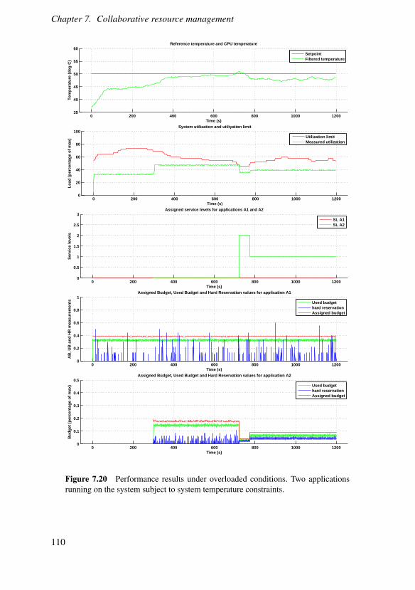
Chapter 7. Collaborative resource management
0 200 400 600 800 1000 120035
40
45
50
55
60Reference temperature and CPU temperature
Time (s)
Tem
per
atu
re (
deg
C)
SetpointFiltered temperature
0 200 400 600 800 1000 12000
20
40
60
80
100System utilization and utiliyation limit
Time (s)
Lo
ad (
per
cen
tag
e o
f m
ax)
Utilization limitMeasured utilization
0 200 400 600 800 1000 12000
0.5
1
1.5
2
2.5
3Assigned service levels for applications A1 and A2
Time (s)
Ser
vice
leve
ls
SL A1SL A2
0 200 400 600 800 1000 12000
0.2
0.4
0.6
0.8
1Assigned Budget, Used Budget and Hard Reservation values for application A1
Time (s)
AB
, UB
an
d H
R m
easu
rem
ents
Used budgethard reservationAssigned budget
0 200 400 600 800 1000 12000
0.1
0.2
0.3
0.4
0.5Assigned Budget, Used Budget and Hard Reservation values for application A2
Time (s)
Bu
dg
et (
per
cen
tag
e o
f m
ax)
Used budgethard reservationAssigned budget
Figure 7.20 Performance results under overloaded conditions. Two applicationsrunning on the system subject to system temperature constraints.
110
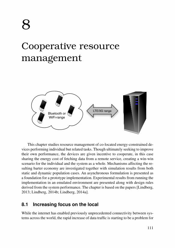
8Cooperative resourcemanagement
LTE/3G rangeBluetooth orWiFi-range
This chapter studies resource management of co-located energy-constrained de-vices performing individual but related tasks. Though ultimately seeking to improvetheir own performance, the devices are given incentive to cooperate, in this casesharing the energy cost of fetching data from a remote service, creating a win-winscenario for the individual and the system as a whole. Mechanisms affecting the re-sulting barter economy are investigated together with simulation results from bothstatic and dynamic population cases. An asynchronous formulation is presented asa foundation for a prototype implementation. Experimental results from running theimplementation in an emulated environment are presented along with design rulesderived from the system performance. The chapter is based on the papers [Lindberg,2013; Lindberg, 2014b; Lindberg, 2014a].
8.1 Increasing focus on the local
While the internet has enabled previously unprecedented connectivity between sys-tems across the world, the rapid increase of data traffic is starting to be a problem for
111
Chapter 8. Cooperative resource management
the network infrastructure [FCC, 2010]. As a result, available wireless broadbandspectrum is quickly being depleted, forcing a renewed focus on finding solutionsthat do not rely on limited infrastructure resources. This is also a relevant strategywhen deploying solutions in previously undeveloped areas, e.g. rural Africa.
While battery capacity is steadily increasing, the desire to create both smallerand more powerful mobile systems continue to be a driver in mobile systems design.Technologies for very energy efficient short range networking are active researchtopics which receive significant attention from device manufacturers.
Mesh networkingIEEE 802.11s, a recent addition to the IEEE 802.11 family of standards, specifiesa way that nodes can form an ad-hoc network and communicate with each otherusing a specialized routing protocol, the Hybrid Wireless Mesh Protocol (HWMP).Private communications between peers, or Mesh Stations as they are called in thestandard, is conducted over encrypted links using a key exchange protocol calledSimultaneous Authentication of Equals (SAE), which is also specifically designedto be used with IEEE 802.11s implementations.
Bluetooth Low EnergyBluetooth Low Energy (BTLE, originally Nokia Wibree) is an addition to the Blue-tooth Core Specification detailing enhanced features for short range communica-tion, including device discovery and peer to peer connectivity. Support for BTLE isalready present in the major mobile operating systems, including Apple iOS, An-droid and Windows Mobile, but the Bluetooth SIG is expecting the technology toalso be used for more specialized devices, e.g. health monitors.
8.2 Incentivizing cooperation
It can be shown through game theory that two rational decision makers will choosenot to cooperate if there is the possibility of one of them taking advantage of theother. This case is often referred to as the “Prisoner’s Dilemma” [Axelrod, 2006]and illustrates the importance of trust between parties in a voluntary cooperationscenario.
Translated into the terms of a cooperative file retrieval scenario, if two geo-graphically co-located mobile clients, A and B, seek to retrieve two data objectsboth clients want from a remote service (typically a file server), they could poten-tially cooperate by sharing the cost, in terms of energy or traffic fees, for the longdistance traffic.
Let wl denote the cost of accessing the data from a remote source and ws thecost of communicating with a co-located source. Accessing data requires energyexpenditure by both sender and receiver, meaning that one local access incurs a cost
112

8.2 Incentivizing cooperation
Table 8.1 Action/reward table for the Prisoner’s Dilemma description of the shar-ing scenario.
Cost for (A,B) B cooperative B uncooperativeA cooperative (wl +2ws, (2wl +ws,
wl +2ws) wl +ws)A uncooperative (wl +ws, (2wl ,2wl)
2wl +ws)
of ws for both parties. The energy expended by the remote server is not accountedfor in this example. Assume also that wl � ws.
A and B can now independently choose to either be cooperative, that is, allowingthe other party to copy a data object, or uncooperative, that is, not giving the otherclient access. The outcome of the possible scenarios in terms of cost to retrieve bothobjects are listen in Table 8.1.
If both choose to cooperate, the costs will consist of one repository access tofetch one object and then two short range accesses, one to deliver the object to thepeer and one to fetch the other object from the same. In case only one chooses tocooperate, both will start out fetching one object from the repository, but only onewill be able to fetch from its peer. The other will then have to perform anotherrepository access to complete the set.
The Nash equilibrium [Axelrod, 2006] of this game is that both A and B chooseto be uncooperative. Two principle strategies can be seen that would resolve thisproblem, either
• ws must be reduced to 0, thereby making it “free” to risk cooperation, or
• the off-diagonal choices must be eliminated, making it impossible for oneparty to exploit the other.
The first strategy models the behavior of traditional peer-to-peer networks,where sharing is considered to be without cost [Androutsellis-Theotokis et al.,2004]. Even if a participant is taken advantage of the majority of the time, theoccasional win is achieved at no cost. In the mobile setting, the risk of runningout of energy or loosing contact with surrounding parties makes such assumptionsunrealistic.
It is therefore necessary that the exchange system provides potential participantswith guarantees that the benefits outweigh the costs. In the general case, this wouldrequire appropriate models for user behavior, which is outside the scope of thisthesis. A simpler scenario can be achieved by requiring that all transactions arebilaterally either cooperative or uncooperative, thereby effectively resorting to thesecond strategy above.
The question of whether or not to allow multicast transfers is problematic. Whilepublications have shown that this improves the efficiency of cooperation [Wolfson
113
Chapter 8. Cooperative resource management
et al., 2007; Yaacoub et al., 2012], there is the risk that clients will opt out of theexchange system and just listen to multicasts, essentially re-introducing a Prisoner’sDilemma like situation. This work therefore assumes that all communication is uni-cast between two parties.
Furthermore, it is assumed that an exchange system can enforce the adherenceto agreements between clients, which will in the case of data object exchanges bereferred to as fair exchanges. Exactly how this is done is of less importance tothe results presented, but for the sake of feasibility a prototype method is outlinedbelow.
Prototype contract mechanismAssume a set of parties C have agreed to exchange a set of objects D according tosome scheme. The agreement, or contract, in the form of a list of tuples denoting(supplier, receiver, object) ∈ C×C×D, is handed over to an exchange system E,a physical 3rd party in the form of a remote service. E creates a set of encryptionkeys, one for each unique object in the agreement. The suppliers of each object arethen given the corresponding keys, which they then use to encrypt the objects, afterwhich they transmit them. When all receivers have signaled to E that they haveindeed received the complete transmissions, E sends out the appropriate decryptionkeys to the participants.
8.3 System model
Consider a population of mobile terminals capable of multi-mode communication,that is, able to use several wireless communication standards. Specifically, they sup-port both an expensive form of long range communication (e.g. 3G or LTE) and aless expensive short range alternative (e.g. WLAN or Bluetooth). Building on thenotation introduced in Section 8.2, let C = {ci, i = 1 . . .Nc} denote a subset of thepopulation, such that all are within short range communication distance of eachother. Furthermore, let D = {d j, j = 1 . . .Nd} denote a set of data objects of uniformsize that all clients desire to retrieve. These objects could be individual files or partsof one larger file, split into parts to facilitate distribution. While constraining the di-vision to equally sized parts can seem like a simplification, it does help to make themarket more efficient. If all parts require equal effort to exchange, finding suitabletrade partners becomes easier.
All parts of D are available from a central repository accessible only over longrange communication. The nominal cost for a client to download all parts of D isthus Ndwl but clients can cooperate by trading objects via short range communica-tion and thereby reduce their total transfer cost. Because of the cost associated withsharing a data object with another client, it is assumed that a client will only providea requested object if it is guaranteed to get an object in return, referred to as a fairexchange. This rule is referred to as the exchange policy.
114
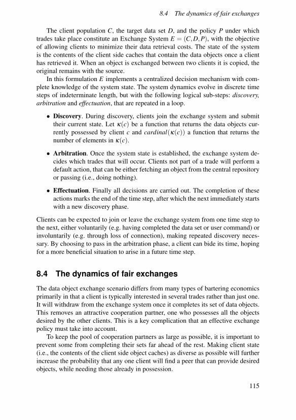
8.4 The dynamics of fair exchanges
The client population C, the target data set D, and the policy P under whichtrades take place constitute an Exchange System E = (C,D,P), with the objectiveof allowing clients to minimize their data retrieval costs. The state of the systemis the contents of the client side caches that contain the data objects once a clienthas retrieved it. When an object is exchanged between two clients it is copied, theoriginal remains with the source.
In this formulation E implements a centralized decision mechanism with com-plete knowledge of the system state. The system dynamics evolve in discrete timesteps of indeterminate length, but with the following logical sub-steps: discovery,arbitration and effectuation, that are repeated in a loop.
• Discovery. During discovery, clients join the exchange system and submittheir current state. Let κ(c) be a function that returns the data objects cur-rently possessed by client c and cardinal(κ(c)) a function that returns thenumber of elements in κ(c).
• Arbitration. Once the system state is established, the exchange system de-cides which trades that will occur. Clients not part of a trade will perform adefault action, that can be either fetching an object from the central repositoryor passing (i.e., doing nothing).
• Effectuation. Finally all decisions are carried out. The completion of theseactions marks the end of the time step, after which the next immediately startswith a new discovery phase.
Clients can be expected to join or leave the exchange system from one time step tothe next, either voluntarily (e.g. having completed the data set or user command) orinvoluntarily (e.g. through loss of connection), making repeated discovery neces-sary. By choosing to pass in the arbitration phase, a client can bide its time, hopingfor a more beneficial situation to arise in a future time step.
8.4 The dynamics of fair exchanges
The data object exchange scenario differs from many types of bartering economicsprimarily in that a client is typically interested in several trades rather than just one.It will withdraw from the exchange system once it completes its set of data objects.This removes an attractive cooperation partner, one who possesses all the objectsdesired by the other clients. This is a key complication that an effective exchangepolicy must take into account.
To keep the pool of cooperation partners as large as possible, it is important toprevent some from completing their sets far ahead of the rest. Making client state(i.e., the contents of the client side object caches) as diverse as possible will furtherincrease the probability that any one client will find a peer that can provide desiredobjects, while needing those already in possession.
115
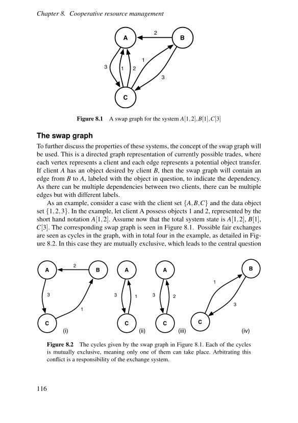
Chapter 8. Cooperative resource management
A
C
B
1
3
2
3 1 2
Figure 8.1 A swap graph for the system A[1,2],B[1],C[3]
The swap graphTo further discuss the properties of these systems, the concept of the swap graph willbe used. This is a directed graph representation of currently possible trades, whereeach vertex represents a client and each edge represents a potential object transfer.If client A has an object desired by client B, then the swap graph will contain anedge from B to A, labeled with the object in question, to indicate the dependency.As there can be multiple dependencies between two clients, there can be multipleedges but with different labels.
As an example, consider a case with the client set {A,B,C} and the data objectset {1,2,3}. In the example, let client A possess objects 1 and 2, represented by theshort hand notation A[1,2]. Assume now that the total system state is A[1,2], B[1],C[3]. The corresponding swap graph is seen in Figure 8.1. Possible fair exchangesare seen as cycles in the graph, with in total four in the example, as detailed in Fig-ure 8.2. In this case they are mutually exclusive, which leads to the central question
A
C
B
3
2
1
A
C
3 1
(i) (ii)
A
C
3 2
(iii)C
B
(iv)
3
1
Figure 8.2 The cycles given by the swap graph in Figure 8.1. Each of the cyclesis mutually exclusive, meaning only one of them can take place. Arbitrating thisconflict is a responsibility of the exchange system.
116

8.4 The dynamics of fair exchanges
Nc
3.03.5
4.04.5
5.05.5
6.0
Nd
3.03.5
4.04.5
5.05.5
6.0
avg c
ycl
es
50
100
150
200
250
300
Figure 8.3 The number of cycles grows very fast with the dimensions of the sys-tem. This plot shows the average number of cycles over 50 simulations when allclients are assigned randomly chosen states.
of arbitration, that is, determining which exchanges should take place in order tooptimize the objectives?
In its entirety, the problem is a multistep decision problem, where in each stepdetermining the set of exchanges to perform involves finding the best set of non-overlapping cycles in the graph, a version of the classic NP-complete maximum setpacking problem [Karp, 1972]. It has been shown how such problems can be solvedthrough relaxation techniques after conversion to the maximum clique formulation[Ausiello et al., 1980; Balas et al., 1996], and this could theoretically provide amethod to solve the complete problem, though the effects of the relaxation on thisproblem is currently unknown, as the goal is not the same as in maximum set-packing.
The computational complexity in each step grows as 2Ncycles and since the num-ber of cycles grows very fast with the set size, as shown in Figure 8.3, finding theglobally optimal solution is intractable for realistic scenarios involving hundreds ofclients. However, a possible key to alternative heuristic strategies presents itself bystudying the special case of Nc = Nd .
117

Chapter 8. Cooperative resource management
A
C
B
3
1
2
(i)
A
C
B
2
3
1
(ii)
Figure 8.4 Swap graphs for the special case discussed in Section 8.4. The systemis initialized with the state A[1],B[2],C[3], as shown in Graph (i), which allows for a3-way exchange involving all clients, leading to the situation depicted in Graph (ii).
The case of Nd = Nc
Consider a case with Nc = Nd = 3, with the system state A[1], B[2], C[3] and thecorresponding swap graph shown in Figure 8.4-i. After trivially selecting the ex-changes, the state becomes A[1,3], B[1,2], C[2,3], with the swap graph in Figure8.4-ii. This gives another trivial decision that ends the scenario (as all clients aredone) with an optimal cost of exactly one remote access for all clients.
The two following observations can now be made:
1. The trivial optimal strategy above is always possible when all clients have thesame number of objects and every object occurs the same number of times inthe system.
2. The solution is not unique in general, there might be many other ways toachieve the same optimal global cost.
Letnc = cardinal(κ(c))
andfd = ∑
c∈CId(c)
where Id(c) is an indicator function defined as
Id(c) =
{0 if d 6∈ κ(c)1 if d ∈ κ(c)
nc is thus the number of objects possessed by c and fd the number of clientspossessing object d. Furthermore, let
n =1
Nc∑c∈C
nc and f =1
Nd∑
d∈Dfd
118

8.5 Baseline algorithm
Using this notation, the condition from Observation 1 can be formalized into
ni = n j,∀i, j ∈C and fk = fl ,∀k, l ∈ D (8.1)
from here on referred to as Condition A.Consider now the function
J = ∑c∈C
(nc− n)2 + ∑d∈D
( fd− f )2 (8.2)
The quantity J can be seen to denote the distance to Condition A, or if it is assumedthat the optimal trajectory will be followed once A is fulfilled, the distance to theoptimal trajectory.
The quantities ∑c∈C(nc− n)2 and ∑d∈D( fd− f )2, essentially the sample varianceof the client cache sizes and object frequencies respectively, can be interpreted tomodel two aspects of how well the exchange system will work.
If the cache size variance is high, then some clients will finish way ahead ofothers, thereby removing many objects from the system. It therefore makes sense toprioritize clients with few objects when arbitrating exchanges.
If the frequency variance is high, some objects are rare, meaning few clients canoffer them, while some are frequent, meaning few clients want them. Both caseswill lead to fewer possible exchanges involving these objects. It therefore makessense to try to keep object frequencies uniform.
Analysis of J’s impact on tradingTo further demonstrate the correlation between the quantity J and number of tradingopportunities, Figure 8.5 shows the result of a Monte-Carlo type simulation wherea system state was generated 5000 times by randomly placing Nd/2 objects amongNc clients, for Nd = Nc = 8. For each random state, the swap graph was constructedand the number of cycles, i.e., the number of possible trades, were plotted againstthe corresponding value of J.
The negative impact on possible trades for high values of J is clear but forsmaller values of J, the correlation grows weaker. It can therefore be expected thatthe algorithm presented in 8.5, which is based on this metric, will primarily workto prevent particularly bad trades, but that it will perform more or less on par withpicking trades at random when the system is close to optimum.
8.5 Baseline algorithm
Using Equation (8.2), it is possible to formulate a one-step decision algorithm basedon minimizing J. Basing decisions on only the currently measurable state of thesystem, in this case the contents of the client side caches, is a feedback control ap-proach. This has the advantage of being robust to disturbances, such as failed trans-fers or clients arriving to or departing from the exchange system. A pre-calculated
119
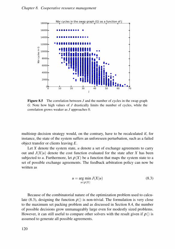
Chapter 8. Cooperative resource management
0 10 20 30 40 50 60 70J
0
2000
4000
6000
8000
10000
12000
14000
16000
18000
Nbr
cycl
es
in G
Nbr cycles in the swap graph (G) as a function of J
Figure 8.5 The correlation between J and the number of cycles in the swap graphG. Note how high values of J drastically limits the number of cycles, while thecorrelation grows weaker as J approaches 0.
multistep decision strategy would, on the contrary, have to be recalculated if, forinstance, the state of the system suffers an unforeseen perturbation, such as a failedobject transfer or clients leaving E.
Let X denote the system state, u denote a set of exchange agreements to carryout and J(X |u) denote the cost function evaluated for the state after X has beensubjected to u. Furthermore, let ρ(X) be a function that maps the system state to aset of possible exchange agreements. The feedback arbitration policy can now bewritten as
u = arg minu∈ρ(X)
J(X |u) (8.3)
Because of the combinatorial nature of the optimization problem used to calcu-late (8.3), designing the function ρ() is non-trivial. The formulation is very closeto the maximum set packing problem and as discussed in Section 8.4, the numberof possible decisions grow unmanageably large even for modestly sized problems.However, it can still useful to compare other solvers with the result given if ρ() isassumed to generate all possible agreements.
120

8.6 Heuristic solver
8.6 Heuristic solver
In order to further study this type of exchange system, a simple heuristic solver hasbeen developed. Its main characteristics are that
• it is deterministic, that is, a given state always yields the same decision,
• it will always terminate (i.e., it is dead- and live-lock free),
• it is guaranteed to find at least one exchange unless there are none, which istrivial to test for, and
• it is computationally inexpensive.
Heuristic cycle findingThe heuristic solver uses a steepest decent style graph walking method for findingcycles. Let
Jc(X) =∂J(X)
∂nc(8.4)
Jd(X) =∂J(X)
∂ fd(8.5)
and let G′ be the pruned swap graph, obtained by repeatedly searching G for nodeswith either zero in-degree or zero out-degree, i.e., nodes with either no inbound orno outbound edges, [Godsil et al., 2001], which obviously cannot be part of a cycle.As removing nodes from the graph can cause other nodes to qualify for pruning, theprocedure is repeated until no more nodes can be removed.
As an example, consider the unpruned swap graph shown in Figure 8.6, definedon the data set D = {1,2,3,4} and client set C = {A,B,C,D}. In the first step ofpruning, client C would be removed as it has no inbound edges. Removing C in turnremoves all inbound edges to A, meaning this node would be removed in the nextpruning iteration. As the remaining nodes B and D have both inbound and outboundedges, no further reductions can be made and resulting graph is the pruned swapgraph G′.
It can easily be seen that the all connected subgraphs in G′ contain at least onecycle. As all nodes have outgoing edges with no edges to itself, there are no "deadends" in the graph and since the graph is finite a walk must eventually end up in anode that has been visited before.
Because there can be multiple edges between nodes, the algorithm must keeptrack of both visited nodes and edges. This is done with a data structure called trace,a list of alternating node and edge elements.
A pseudocode representation of the algorithm used for finding cycles is given asAlgorithm 1. Sort() orders elements in a list according to their unique text labels,which is done in order to make the algorithm deterministic. FirstElement() and
121

Chapter 8. Cooperative resource management
C
A B D
33 1
1
2
1
3
2
2
Figure 8.6 An unpruned swap graph on the data set D = {1,2,3,4} and client setC = {A,B,C,D}. No edges are labeled 4 as all clients already possess this object.
LastElement() return the first and last elements of a list respectively and List()creates a list from the arguments. The function gradJ calculates Jc(X) + Jd(X),using for c the end node of the edge and for d the data object associated with theedge. The last operation removes the preamble of the trace, as the initial parts mightnot be part of the cycle.
A heuristic ρ()
Building on the heuristic cycle finder, a heuristic ρ(), denoted ρH(), can then bedefined. Let HeuristicFind be the heuristic cycle finder algorithm defined as Al-gorithm 1. A pseudocode representation of ρH() is shown as Algorithm 2.
The exchange agreements to be carried out are generated by repeatedly search-ing for cycles in G and removing the nodes and associated edges in found cyclesuntil the remaining graph is empty.
Computational complexity While the exact computational complexity of the al-gorithm is difficult to derive, there are ways to find approximate expressions.
The algorithm most often finds cycles of size 2. This comes from that the tradeswith the initial node have a high impact on the cost function, and the second nodein the cycle will therefore often select it as a trade partner. Hence, it will take inthe order of Nc/2 arbitration steps before the swap graph is empty. Each arbitrationinvolves calculating the gradient of the cost function for all edges going out fromthe current node, move to the most beneficial one, and repeat until arriving at apreviously visited node. Assuming cycles of size 2, this will happen twice for each
122

8.6 Heuristic solver
Input: pruned swap graph G′
Output: a cycle in G′
begincurrent ← FirstElement(Sort(GetNodes(G′)))trace← List(current)done← falsewhile not done do
Es← Sort(GetOutEdges(current))Gs← List()mingrad ← MaxFloat()foreach e in Es do
v← SourceNode(e)d ← DataObject(e)u← ReceiverNode(e)if GradJ(v, d, u) < mingrad then
next ← vmingrad ← GradJ(v, d, u)
endendappend d to traceif next in trace then
done← trueelse
current ← nextendappend next to trace
endwhile FirstElement(trace) 6= LastElement(trace) do
remove first element from traceendreturn trace
end
Algorithm 1: Pseudocode representation of the heuristic cycle finder.
arbitration.Figuring the number of edges from each node is more difficult, as this varies
greatly depending on system state (see Figure 8.5). A theoretical upper bound foroutbound edges for one node is (Nc− 1)(Nd − 1), i.e., the client needs all objectsbut one and all other client have those objects. This has to be done once for eachnode in the cycle, which for the worst case is 2 nodes.
It can thus be concluded that the complexity of finding all trades in one arbitra-tion phase is bounded by Nc(Nc−1)(Nd−1).
123

Chapter 8. Cooperative resource management
Input: A swap graph GOutput: A list of traces representing exchange agreementsbegin
u← List()done← falsewhile not done do
G′← Prune(G)upart← List()if not G′ empty then
upart← HeuristicFind(G′)else
done← trueendremove nodes in upart from Gappend upart to u
endreturn u
end
Algorithm 2: Pseudocode representation of the heuristic decision function ρH()where HeuristicFind() is a call to Algorithm 1.
Default actionsThe clients not part of any exchange are still able to act, though their actions arelimited to either
• fetching an object from the remote repository, or
• passing (i.e., doing nothing).
The decision comes down to if the client is willing to wait and see if a better situationarises or if it should instead pay for immediate access to a data object. In this work,this is modeled by a client parameter named trade timeout that decides how long aclient that is not part of any exchange agreement after arbitration is willing to wait,essentially a form of time out. An important special case arises when a client entersthe exchange system with an empty cache. It will then have to download at least oneobject from the remote repository in order to have something to trade with.
As the other parts of the algorithm aim to minimize J, it would seem appropriatethat the default actions do the same. This can be most easily done by simply fetchingthe least frequent object currently not already possessed by the client. In order topreserve determinism, the candidates are sorted by frequency first and label second.
Example: Empty initial state To further illustrate how the proposed mechanismworks, here follows a step by step execution of the algorithm for a simple case. The
124
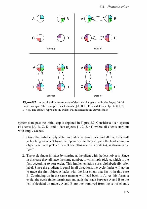
8.6 Heuristic solver
State (a) State (b)
State (c) State (d)
12
3
4
12
12
43
43
12
43
12
43
12
43
12
43
123
123
143
143
A
C
B
D
A
C
B
D
A
C
B
D
A
C
B
D
Figure 8.7 A graphical representation of the state changes used in the Empty initialstate example. The example uses 4 clients ({A, B, C, D}) and 4 data objects ({1, 2,3, 4}). The arrows represent the trades that resulted in the current state.
system state past the initial step is depicted in Figure 8.7. Consider a 4 x 4 system(4 clients {A, B, C, D} and 4 data objects {1, 2, 3, 4}) where all clients start outwith empty caches.
1. Given the initial empty state, no trades can take place and all clients defaultto fetching an object from the repository. As they all pick the least commonobject, each will pick a different one. This results in State (a), as shown in thefigure.
2. The cycle finder initiates by starting at the client with the least objects. Sincein this case they all have the same number, it will simply pick A, which is thefirst according to sort order. This implementation sorts alphabetically afterlabel. Since the gradient is equal in all directions, the cycle finder will go onto trade the first object A lacks with the first client that has it, in this caseB. Continuing on in the same manner will lead back to A. As this forms acycle, the cycle finder terminates and adds the trade between A and B to thelist of decided on trades. A and B are then removed from the set of clients,
125

Chapter 8. Cooperative resource management
A 12 23
14 143
B
C D
A 12 23
14 143
B
C D
3
2
4
State (a) State (b)
Figure 8.8 A graphical representation of the state changes used in the Non-emptyinitial state example. The example uses 4 clients ({A, B, C, D}) and 4 data objects({1, 2, 3, 4}).
a new swap graph is generated and the procedure is repeated, finding a tradebetween the two remaining clients, C and D. After carrying out the trades, thesystem ends up in State (b).
3. Because the gradient is still the same in all directions, the system will con-tinue to pick trades in sort order. This results in A trading with C and B tradingwith D, resulting in State (c).
4. The previous cycles will repeat themselves, resulting trades between the sameclients and the scenario terminates in State (d), as all clients have all dataobjects.
The scenario illustrates how the system can work in an ideal case, where each clientonly needs to fetch one object from the remote server and then trade for the remain-ing.
Example: Non-empty initial state In order to show how the arbitration algorithmpromotes certain trades over others, consider a 4 x 4 system configured in State (a)as shown in Figure 8.8, with client- and data sets as per the previous example.
1. The cycle finder starts with the first client with two objects, which is A. Fromthere it picks the first edge with the lowest object frequency, which is 3, goingto the first node with the lowest object count, which is B. The alternativewould be to trade with D, but because D has more than the average amountof objects, the gradient is positive along this edge.
2. From B, the first edge with the lowest object frequency is 4 and the targetwith the lowest object count is C. Trades with object 1 are not preferred,since object 1 is more common than the average, and client D still has morethan the average number of objects.
126
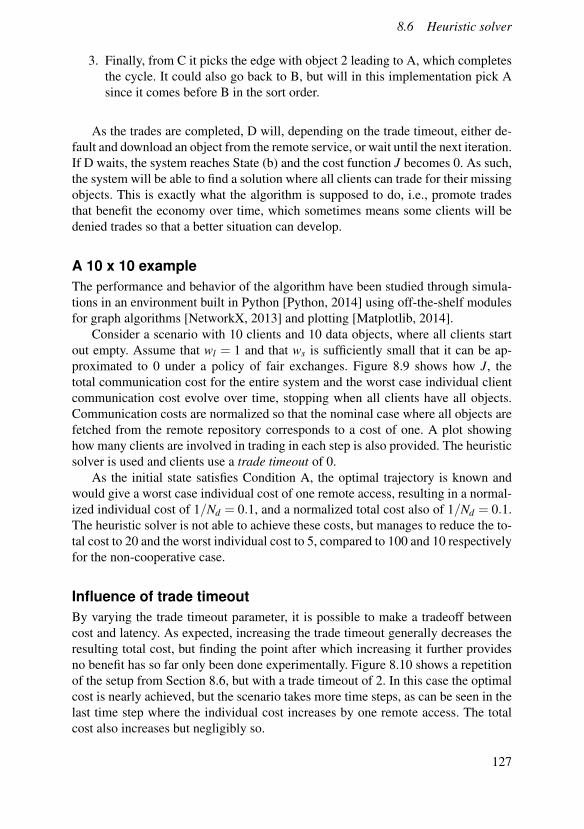
8.6 Heuristic solver
3. Finally, from C it picks the edge with object 2 leading to A, which completesthe cycle. It could also go back to B, but will in this implementation pick Asince it comes before B in the sort order.
As the trades are completed, D will, depending on the trade timeout, either de-fault and download an object from the remote service, or wait until the next iteration.If D waits, the system reaches State (b) and the cost function J becomes 0. As such,the system will be able to find a solution where all clients can trade for their missingobjects. This is exactly what the algorithm is supposed to do, i.e., promote tradesthat benefit the economy over time, which sometimes means some clients will bedenied trades so that a better situation can develop.
A 10 x 10 exampleThe performance and behavior of the algorithm have been studied through simula-tions in an environment built in Python [Python, 2014] using off-the-shelf modulesfor graph algorithms [NetworkX, 2013] and plotting [Matplotlib, 2014].
Consider a scenario with 10 clients and 10 data objects, where all clients startout empty. Assume that wl = 1 and that ws is sufficiently small that it can be ap-proximated to 0 under a policy of fair exchanges. Figure 8.9 shows how J, thetotal communication cost for the entire system and the worst case individual clientcommunication cost evolve over time, stopping when all clients have all objects.Communication costs are normalized so that the nominal case where all objects arefetched from the remote repository corresponds to a cost of one. A plot showinghow many clients are involved in trading in each step is also provided. The heuristicsolver is used and clients use a trade timeout of 0.
As the initial state satisfies Condition A, the optimal trajectory is known andwould give a worst case individual cost of one remote access, resulting in a normal-ized individual cost of 1/Nd = 0.1, and a normalized total cost also of 1/Nd = 0.1.The heuristic solver is not able to achieve these costs, but manages to reduce the to-tal cost to 20 and the worst individual cost to 5, compared to 100 and 10 respectivelyfor the non-cooperative case.
Influence of trade timeoutBy varying the trade timeout parameter, it is possible to make a tradeoff betweencost and latency. As expected, increasing the trade timeout generally decreases theresulting total cost, but finding the point after which increasing it further providesno benefit has so far only been done experimentally. Figure 8.10 shows a repetitionof the setup from Section 8.6, but with a trade timeout of 2. In this case the optimalcost is nearly achieved, but the scenario takes more time steps, as can be seen in thelast time step where the individual cost increases by one remote access. The totalcost also increases but negligibly so.
127
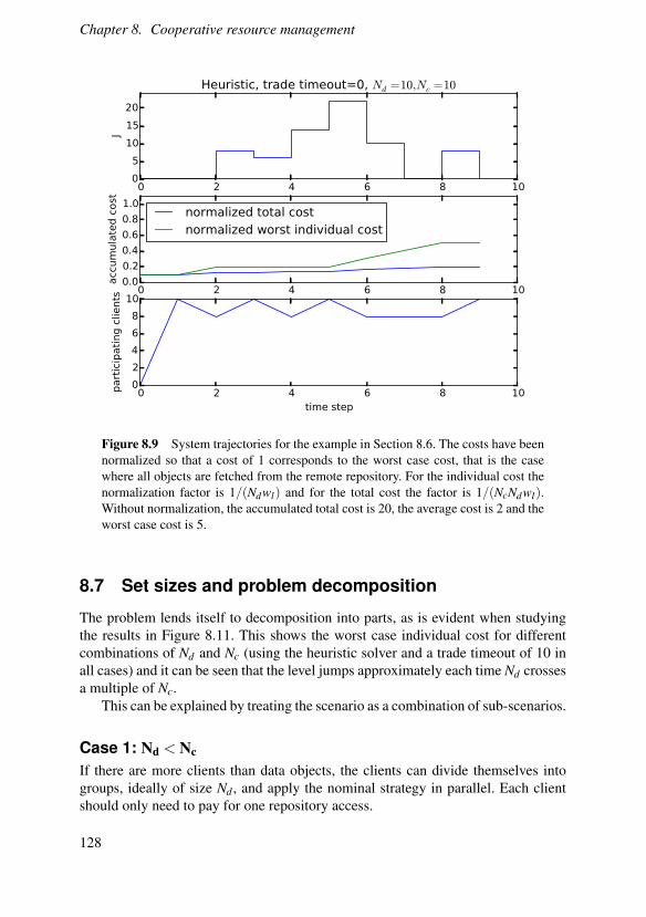
Chapter 8. Cooperative resource management
0 2 4 6 8 10time step
0
5
10
15
20J
Heuristic, trade timeout=0, Nd =10,Nc =10
0 2 4 6 8 10time step
0.0
0.2
0.4
0.6
0.8
1.0
acc
um
ula
ted c
ost
normalized total costnormalized worst individual cost
0 2 4 6 8 10time step
0
2
4
6
8
10
part
icip
ati
ng c
lients
Figure 8.9 System trajectories for the example in Section 8.6. The costs have beennormalized so that a cost of 1 corresponds to the worst case cost, that is the casewhere all objects are fetched from the remote repository. For the individual cost thenormalization factor is 1/(Ndwl) and for the total cost the factor is 1/(NcNdwl).Without normalization, the accumulated total cost is 20, the average cost is 2 and theworst case cost is 5.
8.7 Set sizes and problem decomposition
The problem lends itself to decomposition into parts, as is evident when studyingthe results in Figure 8.11. This shows the worst case individual cost for differentcombinations of Nd and Nc (using the heuristic solver and a trade timeout of 10 inall cases) and it can be seen that the level jumps approximately each time Nd crossesa multiple of Nc.
This can be explained by treating the scenario as a combination of sub-scenarios.
Case 1: Nd < Nc
If there are more clients than data objects, the clients can divide themselves intogroups, ideally of size Nd , and apply the nominal strategy in parallel. Each clientshould only need to pay for one repository access.
128
8.7 Set sizes and problem decomposition
0 2 4 6 8 10 12 14time step
0
5
10
15
20
J
Heuristic, trade timeout=2, Nd =10,Nc =10
0 2 4 6 8 10 12 14time step
0.0
0.2
0.4
0.6
0.8
1.0
acc
um
ula
ted c
ost
normalized total costnormalized worst individual cost
0 2 4 6 8 10 12 14time step
0
2
4
6
8
10
part
icip
ati
ng c
lients
Figure 8.10 System trajectories for the example in Section 8.6, with the trade time-out parameter set to 2, resulting in lower individual and total costs at the expense ofmore time steps. Only a single client is forced to do two repository accesses, whichis seen in the slight increase of worst case cost in the final time step. Without normal-ization, the accumulated total cost is 12, the average cost is 1.2 and the worst casecost is 2.
Case 2: Nd > Nc
If there are more data objects than clients, then the data objects can be divided intogroups, ideally of size Nc and handled in serial manner. Each client must pay forone repository access per serial group.
From this it can be concluded that
dNd/Nce (8.6)
is a reasonable predictor for the worst case individual number of remote accessesusing this solver or with words, a group of Nc clients can often cooperate around aset of Nd objects allowing each client to only pay for once remote repository access.If the remainder is non zero, some clients are likely to be prohibited from tradingfor one object, thereby raising the worst case number of accesses by one. Becauseof the above listed decomposition properties of the problem, (8.6) is also the lowerbound on the worst case communication cost.
129

Chapter 8. Cooperative resource management
Nc
5 10 15 20 25 30 35
Nd
510
1520
2530
35
Max c
ost
1
2
3
4
5
6
7
0 5 10 15 20 25 30 35Nc
0
5
10
15
20
25
30
35
Nd
Figure 8.11 The worst case individual costs (non-normalized) for scenarios of var-ious sizes, all using trade timeout of 10 which has experimentally been proven suffi-cient for all the cases in this simulation to reach their lowest costs. wl is set to 1 (i.e.,the cost is the same as the number of repository accesses), with the plot shown bothfrom the side and from above to make the cost breakpoints more visible.
Variations on the cost functionIt is natural to consider a more general structure on the cost function. ExtendingEquation (8.2) with the weights p and q gives the form
J = p ∑c∈C
(nc− n)2 +q ∑d∈D
( fd− f )2 (8.7)
which can then be used to investigate the influence of the different parts. In order toshow the effects clearly, a system with a skew object distribution state, both in termsof objects possessed by the clients and the frequency of the objects, will be used.For example, let the client set be C = {A, . . . ,J} and the data set be D = {1, . . . ,10}.Table 8.2 describes the initial state, where ’x’ in position (i, j) signifies that client ihas a copy of object j, that is, ∀i, j; j≤ i≤max(i)−2. A set-up of this type will bereferred to as a skew 10x10 system. The reason the state matrix is not diagonal in thetraditional way is that some clients would start with all objects already in possessionand others so close to being finished that the influence of the cost function wouldbe diminished.
Figures 8.12 and 8.13 shows the resulting costs for all clients to complete theirdata sets in skew 10x10 and 20x20 scenarios respectively, with the trade timeout setto 5. The balanced cost function with (p,q) = (1,1) out-performs the alternativesexcept for the case where (p,q) = (10,1) for the 10x10 example. The influence ofthe cost function is reduced for smaller problems, where the combinatorial natureof the problem is more dominant, and for cases where the trade timeout is very low.
130

8.7 Set sizes and problem decomposition
A x x x x x x x x . .B x x x x x x x . . .C x x x x x x . . . .D x x x x x . . . . .E x x x x . . . . . .F x x x . . . . . . .G x x . . . . . . . .H x . . . . . . . . .I . . . . . . . . . .J . . . . . . . . . .
1 2 3 4 5 6 7 8 9 10
Table 8.2 A representation of the skew state used to examine the effect of the pand q parameters in the generalized cost function. An ’x’ on position (i, j) signifiesthat client i has a copy of object j.
(1,1) (10,1) (1,10) (0,1) (1,0)(p,q)
0
2
4
6
8
10
12
cost
(lo
ng r
ange a
ccess
es)
Cost functions variants for 10x10 problem
Total costWorst costAverage cost
Figure 8.12 Resulting costs for different choices of (p,q) for skew 10x10 systems.
131

Chapter 8. Cooperative resource management
(1,1) (10,1) (1,10) (0,1) (1,0)(p,q)
0
5
10
15
20
25
30
cost
(lo
ng r
ange a
ccess
es)
Cost functions variants for 20x20 problem
Total costWorst costAverage cost
Figure 8.13 Resulting costs for different choices of (p,q) for skew 20x20 systems.
Comparison with a feed forward approachThe method presented in [Yaacoub et al., 2012] shows results with energy savingsfrom approximately 60% (unicast case) to 95% (multicast case), when sufficientlymany clients are involved. The results are not immediately comparable with thosepresented in this thesis, as the energy consumption of the IEEE 802.11b WiFi trafficis not sufficiently low to justify the assumption that wl � ws. However, the newerIEEE 802.11n standard has been shown to be in the order of a factor 10 times asefficient in J / bit as 802.11b [Halperin et al., 2012], making the assumption morerealistic.
Using (8.6) as a predictor for the number of repository accesses, the cost todownload Nd objects can be written as
dNd/Ncewl +2(Nd−dNd/Nce)ws (8.8)
Assuming ws is low enough to be negligible and normalizing with the nominal costof Ndwl , the predicted normalized cost under the mechanism proposed in this thesisis dNd/Nce/Nd , meaning that given Nc ≥ Nd , the cost scales with 1/Nd . As such thepredicted energy savings are on par with those presented in [Yaacoub et al., 2012],but note that those results would also be better if IEEE 802.11n had been used.
132

8.8 Random initial state
Nc
4 6 8 10 12 14 16
Nd
46
810
1214
16
avg m
ax c
ost
2
3
4
5
6
Figure 8.14 Average worst case individual cost over 20 simulations using a tradetimeout of 10.
The main advantage of the feedback method in this thesis is that it does notrequire off-line optimization and therefore is able to handle uncertainties better, asshow in Section 8.8.
8.8 Random initial state
Relaxing the assumption on the initial system state will give further insight into howthe feedback based solver will handle a more realistic scenario. Clients might enterthe system with some data objects already collected, others might join with emptycaches at a later stage. Since the algorithm assumes all relevant information is partof the current system state, the exact events leading up to this point are irrelevant.
The result of a sequence of simulations, 20 for each (Nd ,Nc) pair, Figure 8.14shows the average max cost in a system with a random initial state, where eachclient possesses a random number of objects (uniformly distributed in [0,Nd ]). Theobjects are in each case also picked at random, with uniform probability.
On average, a client in these simulations enters the system with half of the ob-
133
Chapter 8. Cooperative resource management
jects already in possession. It would therefore be reasonable to expect that the ex-pected max cost would be lower than what the dNd/Nce rule would predict, but thesimulations suggest otherwise. The explanation for this is that some clients finishtheir sets early, thereby forcing others to pay for many repository accesses, whichin turn increases the max costs.
8.9 Continuous operation
The approach presented in this thesis is primarily targeted at scenarios where thepopulation will change over time, thereby making pre-calculated solutions unviable.A performance evaluation was therefore carried out using simulated scenarios for acase where Nd = 16 and with new clients arriving to the system through a Poissonprocess. The birth intensity was then made to increase over time to see how thesystem behaves under varying load. All clients in the simulation are modeled tohave a trade timeout of 10, meaning they are willing to accept some latency in orderto save energy.
Once a client has completed its data set, it will leave the system. The exchangesystem has a hard limit for the maximum number of clients it will accept and clientsarriving when the system is full will simply be denied access and removed fromthe simulation. The limit could come from system resource constraints, such asmemory, concerns about computational complexity and local network congestionor physical limitations, such as the maximum number of people that can reach eachother with bluetooth or that can fit inside a vehicle with a local wireless network.
System capacity and congestionFigure 8.15 shows how a system with a max capacity of 50 behaves under increas-ing arrival rate. The congestion point is very clear, the completion rate will not goabove 3. The reason for this can be understood through the problem decompositionproperties discussed in Section 8.7. As the average cost in this scenario is close to1, the system performs nearly optimally. Therefore, the clients can be considered togroup up in clusters of size Nd , where each cluster will complete its data set withinNd time steps. Each such cluster will therefore result in an average completion rateof 1 and with a maximum system capacity of 50, there can be b50/16c = 3 suchclusters.
By increasing the maximum capacity of the system, more clusters can be formedand this will improve the throughput. Figure 8.16 shows how the completion ratewill continue to match the birth intensity if the max capacity is increased to supportat least 6 complete groups.
Throughput behavior for max capacity levels in between multiples of Nd re-mains difficult to predict. If bNc/NdcNd clients form complete groups, the remain-der should be able to form fractional groups, as described in Section 8.7, therebycontributing with additional throughput. It seems, however, that the inability of the
134
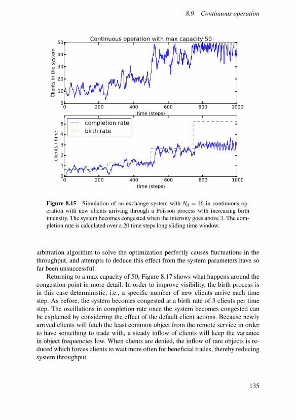
8.9 Continuous operation
0 200 400 600 800 1000time (steps)
0
10
20
30
40
50
Clie
nts
in t
he s
yst
em
Continuous operation with max capacity 50
0 200 400 600 800 1000time (steps)
0
1
2
3
4
5
clie
nts
/ t
ime
completion ratebirth rate
Figure 8.15 Simulation of an exchange system with Nd = 16 in continuous op-eration with new clients arriving through a Poisson process with increasing birthintensity. The system becomes congested when the intensity goes above 3. The com-pletion rate is calculated over a 20 time steps long sliding time window.
arbitration algorithm to solve the optimization perfectly causes fluctuations in thethroughput, and attempts to deduce this effect from the system parameters have sofar been unsuccessful.
Returning to a max capacity of 50, Figure 8.17 shows what happens around thecongestion point in more detail. In order to improve visibility, the birth process isin this case deterministic, i.e., a specific number of new clients arrive each timestep. As before, the system becomes congested at a birth rate of 3 clients per timestep. The oscillations in completion rate once the system becomes congested canbe explained by considering the effect of the default client actions. Because newlyarrived clients will fetch the least common object from the remote service in orderto have something to trade with, a steady inflow of clients will keep the variancein object frequencies low. When clients are denied, the inflow of rare objects is re-duced which forces clients to wait more often for beneficial trades, thereby reducingsystem throughput.
135

Chapter 8. Cooperative resource management
0 200 400 600 800 1000time (steps)
0
20
40
60
80
100
Clie
nts
in t
he s
yst
em
Continuous operation with max capacity 100
0 200 400 600 800 1000time (steps)
0
1
2
3
4
5
clie
nts
/ t
ime
completion ratebirth rate
Figure 8.16 Simulation of an exchange system with Nd = 16 in continuous op-eration with new clients arriving through a Poisson process with increasing birthintensity. The system remains uncongested as intensity goes well above 3. The com-pletion rate is calculated over a 20 time steps long sliding time window.
System designGiven this knowledge about when the system becomes congested, it is possible torelate some of the system design parameters to each other
tstep ≥S(D)
rNd
tc ≤ tstepNd
bmax ≤ bNmax
Ndc
ctot = wl +2(Nd−1)ws
where tstep is the length of a time step in seconds, S(D) the size of the completefile in bits, r the lowest bit-rate used to transfer data either locally or remotely, tcthe time to collect the complete file, bmax the maximum arrival rate to be serviced,Nmax the maximum number of clients in the system and ctot the complete cost ofcollecting the file for each participating client.
136
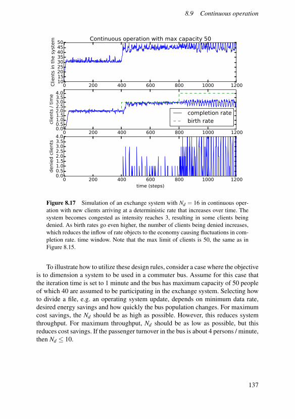
8.9 Continuous operation
0 200 400 600 800 1000 1200time (steps)
101520253035404550
Clie
nts
in t
he s
yst
em Continuous operation with max capacity 50
0 200 400 600 800 1000 1200time (steps)
0.00.51.01.52.02.53.03.54.0
clie
nts
/ t
ime
completion ratebirth rate
0 200 400 600 800 1000 1200time (steps)
0.00.51.01.52.02.53.03.54.0
denie
d c
lients
Figure 8.17 Simulation of an exchange system with Nd = 16 in continuous oper-ation with new clients arriving at a deterministic rate that increases over time. Thesystem becomes congested as intensity reaches 3, resulting in some clients beingdenied. As birth rates go even higher, the number of clients being denied increases,which reduces the inflow of rate objects to the economy causing fluctuations in com-pletion rate. time window. Note that the max limit of clients is 50, the same as inFigure 8.15.
To illustrate how to utilize these design rules, consider a case where the objectiveis to dimension a system to be used in a commuter bus. Assume for this case thatthe iteration time is set to 1 minute and the bus has maximum capacity of 50 peopleof which 40 are assumed to be participating in the exchange system. Selecting howto divide a file, e.g. an operating system update, depends on minimum data rate,desired energy savings and how quickly the bus population changes. For maximumcost savings, the Nd should be as high as possible. However, this reduces systemthroughput. For maximum throughput, Nd should be as low as possible, but thisreduces cost savings. If the passenger turnover in the bus is about 4 persons / minute,then Nd ≤ 10.
137

Chapter 8. Cooperative resource management
8.10 Asynchronous formulation
The synchronous form used in Section 8.6 is not realistic to implement in an actualdistributed system consisting of devices potentially very different from each other,as it relies on a system wide clock and full information available to the central de-cision mechanism. Therefore, this section introduces an asynchronous formulationthat is used as basis for the implementation presented in Section 8.11.
A key difference is the introduction of epochs, here referring to a period in timewhere the decision server accepts connections from clients seeking to participatein the barter, further detailed below. Another significant change is the need to esti-mate the system state, i.e., how many clients are in the system and the contents oftheir caches, something that can potentially affect the effectiveness of the arbitrationalgorithm and the ability of clients to make decisions.
As there is no longer any global period, the trade timeout parameter used tomodel how latency tolerant a client is in the synchronous model is replaced by aquery timeout, specifying how long a client is willing to wait for a trade opportunitybefore taking a default action.
Decision epochsAs one important assumption in this work is the dynamic nature of the client popula-tion, the central decision mechanism can no longer know exactly how many clientsare present and what their intentions are. While the experiments carried out in thiswork uses a fixed client population, the specific clients that connect during eachepoch varies.
As client connections are made, the server collects the incoming queries butwill need to make decisions at some point in time to provide value. This point canbe defined by a number of criteria, such as when a certain number of clients haveconnected, when the estimated system state is within some defined region, or whena predetermined time has passed.
This formulation uses the latter criteria, defining a decision epoch as a period intime of predetermined length, defined by the parameter epoch timeout. Connectionsoccurring after the epoch timeout has occurred are sorted into the next epoch andso on. Once an epoch has been closed, the decision mechanism forms an estimateof the system state based on the client requests made during the epoch time span,as described below, decides which trades should occur, and then communicates outthe results to the clients that are part of that epoch.
System state estimationBecause there is no way to learn the state of clients that have not connected tothe decision server, the system must form an estimate as a basis for decisions. Thetwo main strategies for doing this is to either assume that the clients that connectedduring the current epoch form the entire current population, or model the behavior ofclients and use this to predict how the system state changes. The latter would need to
138
8.11 Software design
include a mobility model, describing how clients move in the physical world, whichis beyond the scope of this thesis. It is also possible to formulate the state estimationas a consensus problem and piggyback state information on trades, something thatwill be necessary for a decentralized formulation.
The estimation technique used in this formulation is to use state informationsubmitted by clients as they connect to the decision server and to also assume thatthey will act optimally, i.e., they will perform the trades decided for them and if theytake a default action, they will choose to fetch the least frequent object, based oncurrent system state estimates. The reason the system is designed in this way, ratherthan having the server explicitly tell the clients what default actions to take, is tomake it possible for clients to make more strategic decisions in a future extensionof this implementation. A client could for instance decide to continue to pass orchange its query timeout based on the information given.
In the current implementation, the state is represented by a list of the labels ofthe data objects that the client currently has cached, e.g. [1,2,5,6,10]. The fact thatthe file is divided into a limited number of predefined parts simplifies the represen-tation of the client state and calculations involving it. If arbitrary parts of the filewould be tradable, not only would the server need to keep a much more detailed de-scription of the contents in each client cache, but finding trades that would benefitall involved parties fairly would also be a much more complex procedure.
8.11 Software design
Using the asynchronous formulation from Section 8.10, a prototype implementationhas been created and tested in a lab environment, as a proof of concept. The deci-sion logic is implemented in Python, a practical high level language for describingcomplex algorithms, while the actual file transfer uses the standard SSH softwaredistributed with most Linux-based operating systems, as this provides the encryp-tion and access control necessary for securing the uni-cast only design while beinga mature and efficient implementation.
Logically, the software consists of a threaded server application implementedusing the Python 3 TCPSocketServer API [Python, 2014], and a client applicationalso written in Python. The server uses the graph software package NetworkX [Net-workX, 2013] for part of the calculations. Figure 8.18 shows an overview of thehardware nodes and how the software components in the system are deployed.
Decision ServerThe decision server implements the central decision mechanism and is the drivingcomponent in the content distribution system. It contains the original copies of thedata objects that the clients seek to retrieve and handles the arbitration of conflictingtrades. It also provides clients with estimates of object frequencies, which the clientsthen can use to make their decisions.
139

Chapter 8. Cooperative resource management
Client
scp
sshd
Server
sshd
query
fetch
fetch
Server Node Client Nodes
Figure 8.18 Component diagram showing the two node types and their softwarecomponents. The Server and Client components are written in Python, while thesshd and scp components are part of the OpenSSH software distribution[OpenSSH,2014].
The server operates in a primary loop where it listens to connections from clientsand sorts them into epochs. When an epoch is closed, arbitration starts while newconnections are accepted in parallel, as seen in Figure 8.19. An important design pa-rameter is the epoch timeout, the choice of which depends on the use case. A largetimeout can allow for many client connections, giving more complete informationabout system state and enabling more trade opportunities, while also incurring morelatency and risking that clients disconnect and perform default actions. A short time-out can reduce latency, but increases the risk that not enough clients will sign intothe system in order to facilitate trades, see Section 8.12.
Client implementationThe clients are relatively primitive, as the primary functionality is implementedusing the SSH-server. The clients work in a single loop:
• First it queries the server, submitting information about the current contentsof its cache in the process.
140

8.11 Software design
Accept Connections
Close Epoch
Create new Epoch
Arbitrate
Reply to clients
Figure 8.19 A diagram of how the main decision server loop operates. The systemstarts by creating a new epoch, which then accepts new client queries until it thetimeout is reached and the epoch is closed. Immediately afterwards, a new epoch iscreated which accepts subsequent client connections, while the arbitration is carriedout in parallel.
• The client then waits for the response until such is received or the client time-out occurs.
• If a trade offer is made, the client enables the trade partner to connect andthen makes its own connection to fetch the suggested data.
• If no answer is given, or if the answer is empty, the client queries the serveragain for information about the object frequencies and then fetches least fre-quent one from the central repository.
Selecting the client query timeout parameter must be done with considerationof epoch timeout, but as is shown in Section 8.12, the effects of different choicescan be non-intuitive as system behavior depends on the activity of all clients, seeSection 8.12.
Energy modelStudies show that mobile phones use significantly different amounts of energy whiletransmitting over different network standards. For instance, using the models pre-
141
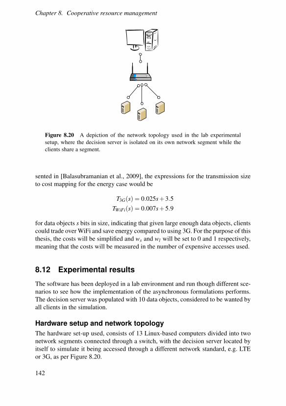
Chapter 8. Cooperative resource management
Figure 8.20 A depiction of the network topology used in the lab experimentalsetup, where the decision server is isolated on its own network segment while theclients share a segment.
sented in [Balasubramanian et al., 2009], the expressions for the transmission sizeto cost mapping for the energy case would be
T3G(s) = 0.025s+3.5TWiFi(s) = 0.007s+5.9
for data objects s bits in size, indicating that given large enough data objects, clientscould trade over WiFi and save energy compared to using 3G. For the purpose of thisthesis, the costs will be simplified and ws and wl will be set to 0 and 1 respectively,meaning that the costs will be measured in the number of expensive accesses used.
8.12 Experimental results
The software has been deployed in a lab environment and run though different sce-narios to see how the implementation of the asynchronous formulations performs.The decision server was populated with 10 data objects, considered to be wanted byall clients in the simulation.
Hardware setup and network topologyThe hardware set-up used, consists of 13 Linux-based computers divided into twonetwork segments connected through a switch, with the decision server located byitself to simulate it being accessed through a different network standard, e.g. LTEor 3G, as per Figure 8.20.
142

8.12 Experimental results
Example run, 5x10To demonstrate how the system works, an example run with five clients,{A,B,C,D,E} and 10 data objects is presented here. The clients start out withempty caches all activate at the same time. Figure 8.21 shows client actions fromepoch to epoch, with ’+’ denoting a trade and ’o’ denoting a default action. Theserver epoch timeout is 3 seconds and the client query timeout is 10 seconds.
As the experiment starts, all clients take a default action as they have nothing totrade with. They then reconnect and clients A-D trade objects with each other duringthe next epoch, while E is not offered a trade as the solver fails to find a cycle inthe graph including it. At about 15 seconds into the experiment, all clients havethe 5 objects fetched during the initial default actions, so no more trades can takeplace. However, as the client does not know that no more clients will connect, theywait, remaining passive until around the 24 second-mark when their query timeoutsoccur. This leads to another round of default actions that opens up for more trades.
The corresponding estimate of J is shown in Figure 8.22, together with an a-posteriori evaluation based on the client side logs. The latter is done by collectingthe individual client logs after the experiment is done and parse the state evaluation.Note how the estimate is consistently higher than the calculated value, a phenomenathat comes from that estimates are formed with no information from one or moreclients, or old information in case queries have timed out and the clients had takena default action. A spike in estimate error occurs around 25 seconds, at a momentwhen many of the clients have timed out and taken default actions. The server isthen forced to form the state estimate without recent information from many of theclients.
Example run, 12x10, long query timeoutThe scenario is similar when scaling up to 12 clients, though because there are nowat least as many clients as there are objects, the mid-scenario pause seen in theprevious example is not present, as can be seen in Figure 8.23. For this experiment,all computers in the lab setup were used, making Nc = 12. The pause is eliminatedbecause all objects are actually possessed by at least one of the clients once theinitial fetch is completed. The long timeout gives the system ample time to findtrades, which in this case results in no extra default actions taken. As the clientdecisions are in this case completely timed by the server, the system essentiallybehaves as synchronized. Since no client reach the query timeout, there is no pointin investigating even higher values.
Example run, 12x10, medium timeoutReducing the time out is one way to avoid long breaks in case objects are missingin the population. However, as shown in Figure 8.24, this can result in fewer clientbeing present for arbitration as they are taking default actions, reducing the overallperformance of the trade economy. The query timeout used here is 5 seconds.
143

Chapter 8. Cooperative resource management
0 5 10 15 20 25 30 35 40time (s)
A
B
C
D
E
Clie
nt
lable
s
Client decisions, o = default, + = trade, vertical lines denote epochs
Figure 8.21 A graphical representation of what actions the clients are taking overthe course of the experiment. ’+’ denotes a trade while ’o’ denotes a default action.The vertical lines show the epoch timeouts.
Example run, 12x10, short query timeoutUsing even shorter timeouts intuitively results in more default actions, as shownin Figure 8.25. In this case, the query timeout is 3 seconds, the same as the serverepoch timeout. In this example, the short timeouts lead to a significant increase indefault actions being taken for some clients (e.g. K and L). Using an even shorterquery timeout is questionable, as this may not give the server time to perform thearbitration.
Effects of client timeoutsFor a client seeking to optimize either latency or energy savings, picking an ap-propriate query timeout is important. The shorter the timeout, the shorter time theclient will be waiting for a trade opportunity. However, because trade opportunitiesare most easily found when many clients with diverse cache contents are available,signing in to the trade system at the same time as the rest of the population turns outto often be more significant than the timeout.
Looking at the cost saving part of the experiment, Figure 8.26 shows the worstand best number of expensive long range accesses used by clients for a some dif-ferent choices of query timeouts in scenarios with 10 clients and 12 data objects.As expected, using long timeouts will likely enable clients to trade for most objectsafter the initial default action has been taken, while at lower timeouts, the variancein savings increases.
Table 8.3 shows the time it takes for clients to complete their entire data setgiven different values on their query timeouts. In all cases, the epoch timeout is
144
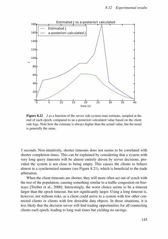
8.12 Experimental results
0 5 10 15 20 25 30 35 40time (s)
0
20
40
60
80
100
120
140
160
180
J
Estimated J vs a-posteriori calculated
Estimated Ja-posteriori calculated J
Figure 8.22 J as a function of the server side system state estimate, sampled at theend of each epoch, compared to an a-posteriori calculated value based on the clientside logs. Note how the estimate is always higher than the actual value, but the trendis generally the same.
3 seconds. Non-intuitively, shorter timeouts does not seems to be correlated withshorter completion times. This can be explained by considering that a system withvery long query timeouts will be almost entirely driven by server decisions, pro-vided the system is not close to being empty. This causes the clients to behavealmost in a synchronized manner (see Figure 8.21), which is beneficial to the tradearbitration.
When the client timeouts are shorter, they will more often act out of synch withthe rest of the population, causing something similar to a traffic congestion on free-ways [Treiber et al., 2000]. Interestingly, the worst choice seems to be a timeoutlarger than the epoch timeout, but not significantly larger. Using a long timeout is,however, not without risks, as a client could arrive to a system with few other con-nected clients or clients with few desirable data objects. In those situations, it isless likely that the decision server will find trading opportunities for all connectingclients each epoch, leading to long wait times but yielding no savings.
145

Chapter 8. Cooperative resource management
0 5 10 15 20 25 30 35time (s)
A
B
C
D
E
F
G
H
I
J
K
LC
lient
lable
s
Client decisions, o = default, + = trade, vertical lines denote epochs
Figure 8.23 A graphical representation of what actions the clients are taking overthe course of the experiment for a case where the query timeout is 10 seconds. ’+’denotes a trade while ’o’ denotes a default action. The vertical lines show the epochtimeouts.
0 5 10 15 20 25 30 35time (s)
A
B
C
D
E
F
G
H
I
J
K
L
Clie
nt
lable
s
Client decisions, o = default, + = trade, vertical lines denote epochs
Figure 8.24 A graphical representation of what actions the clients are taking overthe course of the experiment for a case where the query timeout is 5 seconds. ’+’denotes a trade while ’o’ denotes a default action. The vertical lines show the epochtimeouts.
146
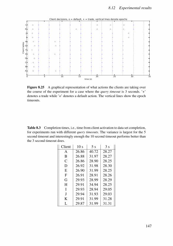
8.12 Experimental results
0 5 10 15 20 25 30 35time (s)
A
B
C
D
E
F
G
H
I
J
K
LC
lient
lable
s
Client decisions, o = default, + = trade, vertical lines denote epochs
Figure 8.25 A graphical representation of what actions the clients are taking overthe course of the experiment for a case where the query timeout is 3 seconds. ’+’denotes a trade while ’o’ denotes a default action. The vertical lines show the epochtimeouts.
Table 8.3 Completion times, i.e., time from client activation to data set completion,for experiments run with different query timeouts. The variance is largest for the 5second timeout and interestingly enough the 10 second timeout performs better thanthe 3 second timeout does.
Client 10 s 5 s 3 sA 26.86 40.72 28.27B 26.88 31.97 28.27C 26.86 28.90 28.25D 26.92 31.98 28.30E 26.90 31.99 28.25F 26.91 28.91 28.26G 29.93 28.99 28.29H 29.91 34.94 28.25I 29.93 28.94 29.05J 29.94 31.93 29.03K 29.91 31.99 31.28L 29.87 31.99 31.31
147

Chapter 8. Cooperative resource management
0.0 0.5 1.0 1.5 2.0 2.5 3.0 3.5timeout (server periods)
0
2
4
6
8
10co
sts
(nbr
of
expensi
ve a
ccess
es)
Completion costs as a function of client query timeout
minimum completion costmaximum completion cost
Figure 8.26 The maximum and minimum costs for a client to complete its data setas a function of the query timeout setting. For high timeout values the performanceis consistent while for lower values it starts to fluctuate. A timeout of 0 means thatthe client always performs a default action.
8.13 Conclusions
This chapter has presented an approach for cooperative content distribution for mo-bile networks with the intent of conserving energy and long range spectrum re-sources. The approach is based on a mechanism where mobile clients trade datain a barter economy-like manner. Trades are arbitrated using a feedback controlapproach, using a cost function shown to correlate to the efficiency of the economy.
The approach is presented in closed population as well as dynamic populationscenarios and an experimental validation through an implementation in a lab envi-ronment is supplied.
148

9Conclusions and futurework
9.1 Conclusions
This thesis presents three different perspectives on feedback-based resource man-agement for cyber-physical systems. The initial viewpoint is the competitive sce-nario, when unrelated components share the same limited resource. The secondviewpoint is the collaborative scenario, where components contribute to the sameperformance metric while sharing a limited and time varying resource. The thirdand final viewpoint is the cooperative scenario, where unrelated clients choose tocooperate around a task to better utilize limited resources.
All scenarios are characterized by limited knowledge of component dynamicsand resource availability, making feedback-based methods an attractive alternativeto overly pessimistic worst case designs. Online event-based estimation techniquesare used to reduce uncertainty and the need for software designers to provide de-tailed information about resource needs.
Convex optimization is used as a mechanism for online decision making in thecompetitive case, while taking care not to expend too much resources on solving theoptimization problem. The feedback-based approach performs worse under condi-tions with perfect knowledge, as some amount of resources are unavoidably usedup by the decision making system and the error when estimating system parameterswill further reduce performance.
Designing for feedbackThe software models used in this thesis have been specifically chosen to enablefeedback resource management. Software components are assumed to have a cyclic,primarily resource dependent, behavior, i.e., the component output is driven by theresources provided as input. This also means restricting software so that it cannottake resource decisions by itself, as this would make estimating the parameters inthe input/output model difficult.
149

Chapter 9. Conclusions and future work
A recurring pattern has also been that resource management decisions are madesmall and assumed to be part of an infinite sequence of actions. This is typicalfor a feedback control approach, especially when including estimation, and thisthesis demonstrates three approaches of how to break down resource managementdecisions in this manner.
Cross domain modelsThe thesis has demonstrated techniques for creating system models that encompassboth physical and computational aspects of a system and how such models canbe used in feedback-based resource management to control performance metricsthat depend on multiple system components. Particular emphasis has been given toincluding energy and thermal properties, as these properties are a common concern,especially in mobile systems. The thermal model is validated through experimentson a mobile robot using adaptive resource management.
The discrete flow model used for resource control in Chapter 7 is applicable toboth computational and physical resource flows. The event like nature of how com-putational resources are generated and consumed is handled through integration,meaning that their effect is well defined over a period of time.
Alternatives to hard real-timeThe absolute guarantees required for hard real-time theory is not suited for the sys-tems studied in this thesis. Neither are the systems mentioned of the type that aresafety critical nor do they require perfect timeliness in order to function. As such,the focus is rather on describing how the performance varies with the allocated re-sources.
This thesis shows how to use rate-based performance metrics for both competi-tive and collaborative resource management and how event-based estimation tech-niques can be used to derive component model parameters online. The synchro-nization example in particular does not fit with the traditional hard/soft real-timeformulations, as there are no deadlines involved in the metric at all.
Resource conservation and green computingReducing energy consumption in devices serves both to enable more advanced mo-bile systems and to build a more sustainable society. This thesis shows both howto explicitly relate power consumption to system metrics for a software system andhow cooperative techniques can be employed to reduce the overall energy consump-tion in a population of co-located devices.
9.2 Future work
The field of cyber-physical systems is still new and much remains to be done inregards to the topics presented in this thesis.
150

9.2 Future work
Modeling of cyber-physical systemsThe cyclic component model used in this thesis lacks the ability to describe morestateful components. Each cycle is assumed to take on average the same amount ofresources, but as shown in the plot regarding rendering time for video frames, thereare patterns that could be exploited for more exact prediction and control.
One possibility is to tie the cycle resource demand to a markov chain model,where each state represents a tighter estimate of the resource need. This would en-able better prediction that would result in better performance for, e.g., synchroniza-tion control.
Competitive resource managementThe components used in this chapter are simplistic and one natural extension is toused composite collaborative components, e.g., the conversational video pipelinefrom Chapter 7. The only constraint is that the utility function is concave, which istrue, e.g., for pipeline throughput.
The potential uses for non-homogeneous utility functions is never explored indetail, though the algorithm does support it. Potential uses for this could be to treatcritical components different than non-critical or to have different utility functionsdepending on the level of system overload.
The algorithm currently does not support multicore resource allocation, as thiswould introduce bin packing-like properties which would not be solvable by a gra-dient descent style algorithm. However, it would be interesting to see how a convexrelaxation of a bin-packing problem could be used to efficiently do approximatelyoptimal resource management on multicore platforms.
Collaborative resource managementIn the example discussed in this thesis, the flows only go from physical (power)to computational (events) but never the other way, thereby never fully realizing thepotential to model the end-to-end performance of an entire physical system. Sucha system would be the result of having computational resources feed into physicalcomponents, e.g., the computational output from a software controller component tothe analog input of a physical device it controls, and studying resource managementfrom energy to controller performance would be an important extension.
Furthermore, the control strategies used in this thesis never uses knowledgeabout the stochastic parts of the model, e.g., the cycle resource requirements, eventhough they are known. Control performance could potentially be enhanced bystochastic control theory, though with special care to handle exponentially dis-tributed disturbances rather than gaussian.
Cooperative resource managementThe current cost function used in the heuristic algorithm could be generalized toprohibit specifically undesirable situations by introducing cross terms. The current
151
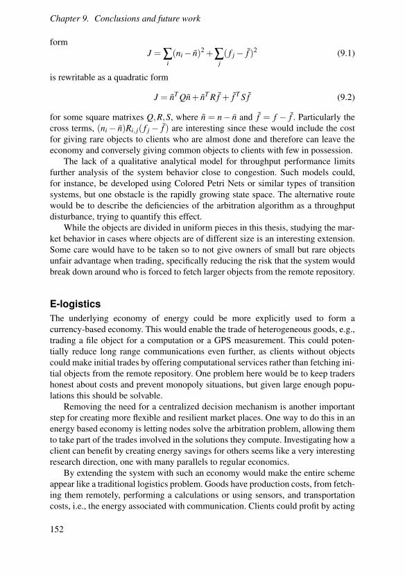
Chapter 9. Conclusions and future work
formJ = ∑
i(ni− n)2 +∑
j( f j− f )2 (9.1)
is rewritable as a quadratic form
J = nT Qn+ nT R f + f T S f (9.2)
for some square matrixes Q,R,S, where n = n− n and f = f − f . Particularly thecross terms, (ni− n)Ri, j( f j− f ) are interesting since these would include the costfor giving rare objects to clients who are almost done and therefore can leave theeconomy and conversely giving common objects to clients with few in possession.
The lack of a qualitative analytical model for throughput performance limitsfurther analysis of the system behavior close to congestion. Such models could,for instance, be developed using Colored Petri Nets or similar types of transitionsystems, but one obstacle is the rapidly growing state space. The alternative routewould be to describe the deficiencies of the arbitration algorithm as a throughputdisturbance, trying to quantify this effect.
While the objects are divided in uniform pieces in this thesis, studying the mar-ket behavior in cases where objects are of different size is an interesting extension.Some care would have to be taken so to not give owners of small but rare objectsunfair advantage when trading, specifically reducing the risk that the system wouldbreak down around who is forced to fetch larger objects from the remote repository.
E-logisticsThe underlying economy of energy could be more explicitly used to form acurrency-based economy. This would enable the trade of heterogeneous goods, e.g.,trading a file object for a computation or a GPS measurement. This could poten-tially reduce long range communications even further, as clients without objectscould make initial trades by offering computational services rather than fetching ini-tial objects from the remote repository. One problem here would be to keep tradershonest about costs and prevent monopoly situations, but given large enough popu-lations this should be solvable.
Removing the need for a centralized decision mechanism is another importantstep for creating more flexible and resilient market places. One way to do this in anenergy based economy is letting nodes solve the arbitration problem, allowing themto take part of the trades involved in the solutions they compute. Investigating how aclient can benefit by creating energy savings for others seems like a very interestingresearch direction, one with many parallels to regular economics.
By extending the system with such an economy would make the entire schemeappear like a traditional logistics problem. Goods have production costs, from fetch-ing them remotely, performing a calculations or using sensors, and transportationcosts, i.e., the energy associated with communication. Clients could profit by acting
152

9.2 Future work
A
B
C
D
E
FG
Figure 9.1 A more general problem structure where clients are divided into co-located subgroups, within each of which short range communication is possible,while only some clients would be close enough to communicate with neighboringgroups.
as distributors, fetching goods from clients out of short range reach of the others(see Figure 9.1). This would require a more explicit model of the spatial relationsbetween clients and the cost function to minimize would need reflect the varyingtotal cost of services. There is likely traditional logistics theory that could apply toa system like that.
153

Bibliography
Abeni, L. and G. Buttazzo (1998a). “Integrating multimedia applications in hardreal-time systems”. In: Proceedings of the 19th IEEE Real-Time Systems Sym-posium (RTSS). Madrid, Spain, pp. 3–13.
Abeni, L. and G. C. Buttazzo (1998b). “Integrating multimedia applications in hardreal-time systems”. In: Proceedings of the 19th IEEE Real-Time Systems Sym-posium (RTSS ’98). Madrid, Spain, pp. 4 –13.
Abeni, L. and G. C. Buttazzo (1999). “Adaptive bandwidth reservation for multime-dia computing”. In: Proceedings of the Sixth International Conference on Real-Time Computing Systems and Applications. IEEE Computer Society, Washing-ton, DC, USA.
Abeni, L., G. Lipari, and G. C. Buttazzo (1999). “Constant bandwidth vs propor-tional share resource allocation”. In: Proceedings of IEEE International Con-ference on Multimedia Computing and Systems (ICMCS ’99). Vol. 2. Florence,Italy, pp. 107 –111.
Abeni, L., L. Palopoli, S. Superiore, and J. Walpole (2002). “Analysis of areservation-based feedback scheduler”. In: Proceedings of the 23rd IEEE Real-Time Systems Symposium (RTSS 2002). Austin, Texas, USA, pp. 71–80.
Akyildiz, I. F., G. Morabito, and S. Palazzo (2001). “Tcp-peach: a new congestioncontrol scheme for satellite ip networks”. IEEE/ACM Trans. Netw. 9:3, pp. 307–321. ISSN: 1063-6692.
Anderson, D. P., S. Tzou, R. Wahbe, R. Govindan, and M. Andrews (1990). “Sup-port for continuous media in the DASH system”. In: Proceedings of the 10 Inter-national Conference on Distributed Computing Systems (ICDC ’90). Berkeley,CA, USA, pp. 54 –61.
Android (2014). Android.com. URL: http://www.android.com.Androutsellis-Theotokis, Stephanos, and D. Spinellis (2004). “A survey of peer-to-
peer content distribution technologies”. ACM Computing Survey 36:4, pp. 335–371. ISSN: 0360-0300.
AQuoSA (2010). URL: http://aquosa.sourceforge.net.
154

Bibliography
Årzén, K.-E. (1999). “A simple event-based PID controller”. In: Proceedings of the14th IFAC World Congress.
Åström, K. J. and R. M. Murray (2008). Feedback systems: an introduction for sci-entists and engineers. Princeton University Press, 41 William Street, Princeton,New Jersey, p. 396.
Ausiello, G., A. D’Atri, and M. Protasi (1980). “Structure preserving reductionsamong convex optimization problems”. Journal of Computer and System Sci-ences 21:1, pp. 136–153.
Axelrod, R. (2006). Evolution of cooperation. Basic Books.Aydin, H., R. Melhem, D. Mosse, and P. Mejia-Alvarez (2001). “Dynamic and ag-
gressive scheduling techniques for power-aware real-time systems”. In: Real-Time Systems Symposium, 2001. (RTSS 2001). Proceedings. 22nd IEEE, pp. 95–105.
Aydin, H., R. Melhem, D. Mosse, and P. Mejia-Alvarez (2004). “Power-awarescheduling for periodic real-time tasks”. Computers, IEEE Transactions on53:5, pp. 584–600. ISSN: 0018-9340.
Balas, E., S. Ceria, G. Cornuéjols, and G. Pataki (1996). “Polyhedral methods forthe maximum clique problem”. Clique, Coloring and Satisfiability: The Sec-ond DIMACS Challenge. The American Mathematical Society, Providence, RI,pp. 11–27.
Balasubramanian, N., A. Balasubramanian, and A. Venkataramani (2009). “Energyconsumption in mobile phones: a measurement study and implications for net-work applications”. In: Proceedings of the 9th ACM SIGCOMM conferenceon Internet measurement conference. IMC ’09. ACM, New York, NY, USA,pp. 280–293. ISBN: 978-1-60558-771-4.
Barham, P., B. Dragovic, K. Fraser, S. Hand, T. Harris, A. Ho, R. Neugebauer, I.Pratt, and A. Warfield (2003). “Xen and the art of virtualization”. SIGOPS Oper.Syst. Rev. 37:5, pp. 164–177. ISSN: 0163-5980.
Bautista, D., J. Sahuquillo, H. Hassan, S. Petit, and J. Duato (2008). “A simplepower-aware scheduling for multicore systems when running real-time applica-tions”. In: Parallel and Distributed Processing, 2008. IPDPS 2008. IEEE Inter-national Symposium on, pp. 1–7.
Bhattacharyya, S. S., G. Brebner, J. W. Janneck, J. Eker, C. von Platen, M. Mat-tavelli, and M. Raulet (2009). “OpenDF: a dataflow toolset for reconfigurablehardware and multicore systems”. ACM SIGARCH Computer Architecture News36:5, pp. 29–35.
Bini, E., G. Buttazzo, J. Eker, S. Schorr, R. Guerra, G. Fohler, K.-E. Årzén, V.Romero Segovia, and C. Scordino (2011). “Resource management on multicoresystems: the actors approach”. IEEE Micro 31:3, pp. 72–81.
Boyd, S. P. and L. Vandenberghe (2004). Convex optimization. Cambridge Univer-sity Press, Cambridge, p. 716.
155
Bibliography
Branicky, M., S. Phillips, and W. Zhang (2002). “Scheduling and feedback co-design for networked control systems”. In: Decision and Control, 2002, Pro-ceedings of the 41st IEEE Conference on. Vol. 2, 1211–1217 vol.2.
Buttazzo, G. C. (1997). Hard real-time computing systems: predictable schedulingalgorithms and applications. Kluwer Academic Publishers, Dordrecht, Nether-lands.
Buttazzo, G. C., M. Spuri, and F. Sensini (1995). “Value vs. deadline schedulingin overload conditions”. In: Proceedings of the 16th IEEE Real-Time SystemsSymposium (RTSS ’95). Pisa, Italy.
Caccamo, M., G. C. Buttazzo, and L. Sha (2000). “Elastic feedback control”. In:12th Euromicro Conference on Real-Time Systems (ECRTS 2000). Stockholm,Sweden, pp. 121–128.
Cervin, A. and T. Henningsson (2008). “Scheduling of event-triggered controllerson a shared network”. In: Decision and Control, 2008. CDC 2008. 47th IEEEConference on, pp. 3601–3606.
Cervin, A. and J. Eker (2003). “The control server: a computational model for real-time control tasks”. In: Proceedings of the 15th Euromicro Conference on Real-Time Systems (ECRTS 2003). Porto, Portugal, pp. 113 –120.
Cervin, A., J. Eker, B. Bernhardsson, and K. Årzén (2002). “Feedback–feedforwardscheduling of control tasks”. Real-Time Systems 23, pp. 23–53.
Cha, H., J. Oh, and R. Ha (2003). “Dynamic frame dropping for bandwidth controlin MPEG streaming system”. Multimedia Tools and Applications 19:2, pp. 155–178.
Chen, G., W. He, J. Liu, S. Nath, L. Rigas, L. Xiao, and F. Zhao (2008). “Energy-aware server provisioning and load dispatching for connection-intensive internetservices.” In: NSDI. Vol. 8, pp. 337–350.
Cheung, T. L., K. Okamoto, F. Maker, X. Liu, and V. Akella (2009). “Markov de-cision process (MDP) framework for optimizing software on mobile phones”.In: Proceedings of the Seventh ACM International Conference on EmbeddedSoftware. ACM, New York, NY, USA, pp. 11–20.
Choudhury, P., P. Chakrabarti, and R. Kumar (2012). “Online scheduling of dy-namic task graphs with communication and contention for multiprocessors”.Parallel and Distributed Systems, IEEE Transactions on 23:1, pp. 126–133.ISSN: 1045-9219.
Coffman Jr., E. G., M. R. Garey, and D. S. Johnson (1997). “Approximation algo-rithms for bin packing: a survey”. In: Approximation algorithms for NP-hardproblems. PWS Publishing Co, Boston, MA, USA, pp. 46 –93.
CGAL (2010). Computational geometry algorithms library. URL: http://www.cgal.org.
156

Bibliography
Cormen, T. H. (2001). Introduction to algorithms. MIT Press, Cambridge, MA,USA, p. 1180.
Cucinotta, T., D. Giani, D. Faggioli, and F. Checconi (2011). “Providing perfor-mance guarantees to virtual machines using real-time scheduling”. In: Euro-Par2010 Parallel Processing Workshops. Springer, pp. 657–664.
D-Bus (2010). URL: http://www.freedesktop.org/wiki/Software/dbus.Daniel E. Rivera, M. M. and S. Skogestad (1986). “Internal model control 4:
pid controller design”. In: Industrial and Engineering Chemestry Research,pp. 252–265.
Delvare, J. (2010). Kernel driver lm83. http://www.mjmwired.net/kernel/Documentation/hwmon/lm83.
Demers, A., S. Keshav, and S. Shenker (1989). “Analysis and simulation of a fairqueueing algorithm”. In: SIGCOMM ’89: Symposium proceedings on Commu-nications architectures & protocols. ACM, New York, NY, USA, pp. 1–12.
Eker, J. and J. W. Janneck (2003). CAL language report. Tech. rep. UCB/ERLM03/48. University of California at Berkeley.
Federal Communications Commission (2010). MOBILE BROADBAND: THE BEN-EFITS OF ADDITIONAL SPECTRUM. Tech. rep. Federal CommunicationsCommission.
Ferreira, A. P., D. Mosse, and J. C. Oh (2007a). “Thermal faults modeling using a rcmodel with an application to web farms”. In: Proceedings of the 19th EuromicroConference on Real-Time Systems (ECRTS 2007). Pisa, Italy, pp. 113–124.
Ferreira, A., D. Mosse, and J. Oh (2007b). “Thermal faults modeling using a rcmodel with an application to web farms”. In: Real-Time Systems, 2007. ECRTS’07. 19th Euromicro Conference on, pp. 113–124.
Foundry, D. (2010). Tech analysis: crackdown 2 demo. URL: http : / / www .eurogamer.net/articles/digitalfoundry-crackdown2-demo-blog-entry.
Fu, Y., N. Kottenstette, Y. Chen, C. Lu, X. D. Koutsoukos, and H. Wang (2010a).“Feedback thermal control for real-time systems”. In: Real-Time and Embed-ded Technology and Applications Symposium (RTAS), 2010 16th IEEE. IEEE,pp. 111–120.
Fu, Y., N. Kottenstette, Y. Chen, C. Lu, X. D. Koutsoukos, and H. Wang (2010b).“Feedback thermal control for real-time systems”. In: Proceedings of the 16thReal-Time and Embedded Technology and Applications Symposium (RTAS2010). Stockholm, Sweden, pp. 111–120.
Geyer, T. (2005). Low Complexity Model Predictive Control in Power Electronicsand Power Systems. English. Cuvillier Verlag, Göttingen, p. 291.
157

Bibliography
Giselsson, P., M. D. Doan, T. Keviczky, B. D. Schutter, and A. Rantzer (2013). “Ac-celerated gradient methods and dual decomposition in distributed model predic-tive control”. Automatica 49:3, pp. 829 –833. ISSN: 0005-1098.
GLPK. Gnu linear programming kit. URL: http://www.gnu.org/software/glpk.
Godsil, C. D., G. Royle, and C. Godsil (2001). Algebraic graph theory. Vol. 8.Springer New York.
Goel, A., J. Walpole, and M. Shor (2004). “Real-rate scheduling”. In: Proceedingsof the 10 IEEE Real-Time and Embedded Technology and Applications Sympo-sium (RTAS 2004). Toronto, Canada, pp. 434 –441.
Golestani, S. J. (1994). “A self-clocked fair queueing scheme for broadband ap-plications”. In: Proceedings of the 13th IEEE Conference on Networking forGlobal Communications (INFOCOM ’94).
Grant, M. and S. P. Boyd (2010). CVX: matlab software for disciplined convex pro-gramming, version 1.21. http://cvxr.com/cvx.
Halperin, D., B. Greensteiny, A. Shethy, and D. Wetherally (2012). “Demystifying802.11n power consumption”. In: Proceedings of the 2010 Workshop on PowerAware Computing and Systems.
Harbour, M. G. (2008). FRESCOR: framework for real-time embedded systemsbased on contracts. URL: http://www.frescor.org.
He, T., J. A. Stankovic, M. Marley, C. Lu, Y. Lu, and T. Abdelzaher (2007). “Feed-back control-based dynamic resource management in distributed real-time sys-tems”. Journal of Systems and Software 80:7, pp. 997–1004.
Henningsson, T. and A. Cervin (2009). “Comparison of LTI and event-based controlfor a moving cart with quantized position measurements”. In: Proceedings of theEuropean Control Conference.
Herrtwich, R. G. (1991). “The role of performance, scheduling and resource reser-vation in multimedia systems”. In: Proceedings of the International Workshopon Operating Systems of the 90s and Beyond. Springer-Verlag, London, UK,pp. 279–284. ISBN: 3-540-54987-0.
Hoffmann, H., J. Eastep, M. D. Santambrogio, J. E. Miller, and A. Agarwal (2010).“Application heartbeats: a generic interface for specifying program performanceand goals in autonomous computing environments”. In: Proceedings of the 7thinternational conference on Autonomic computing. ACM, pp. 79–88.
Intel 64 and IA-32 Architectures Software Developer’s Manual Volume 2A: Instruc-tion Set Reference, A-M (2010). Intel Corporation. Santa Clara, CA, USA.
Isovic, D. and G. Fohler (2004). “Quality aware MPEG-2 stream adaptation in re-source constrained systems”. In: Proceedings of the 16th Euromicro Conferenceon Real-Time Systems (ECRTS 2004). Catania, Italy, pp. 23–32.
158

Bibliography
Jain, R., D.-M. Chiu, and W. R. Hawe (1984). A quantitative measure of fairnessand discrimination for resource allocation in shared computer system. EasternResearch Laboratory, Digital Equipment Corporation.
Jerez, J. L., K.-V. Ling, G. A. Constantinides, and E. C. Kerrigan (2012). “Modelpredictive control for deeply pipelined field-programmable gate array imple-mentation: algorithms and circuitry”. Control Theory & Applications, IET 6:8,pp. 1029–1041.
Jin, X. and Y.-K. Kwok (2010). “Cloud assisted p2p media streaming for band-width constrained mobile subscribers”. In: Parallel and Distributed Systems(ICPADS), 2010 IEEE 16th International Conference on, pp. 800–805.
Jung, E., Y. Wang, I. Prilepov, F. Maker, X. Liu, and V. Akella (2010). “User-profile-driven collaborative bandwidth sharing on mobile phones”. In: Proceedings ofthe 1st ACM Workshop on Mobile Cloud Computing & Services: SocialNetworks and Beyond. MCS ’10. ACM, New York, NY, USA, 2:1–2:9. ISBN:978-1-4503-0155-8.
Kaneko, H., J. A. Stankovic, S. Sen, and K. Ramamritham (1996). “Integratedscheduling of multimedia and hard real-time tasks”. In: Proceedings of the 17thIEEE Real-Time Systems Symposium (RTSS ’96). Washington, DC, USA.
Karp, R. (1972). “Reducibility among combinatorial problems”. English. In: Miller,R. et al. (Eds.). Complexity of Computer Computations. The IBM ResearchSymposia Series. Springer US, pp. 85–103. ISBN: 978-1-4684-2003-6.
Katabi, D., M. Handley, and C. Rohrs (2002). “Congestion control for highbandwidth-delay product networks”. In: Proceedings of the 2002 Conferenceon Applications, Technologies, Architectures, and Protocols for Computer Com-munications. SIGCOMM ’02. ACM, New York, NY, USA, pp. 89–102. ISBN:1-58113-570-X.
Kellerer, H., U. Pferschy, and D. Pisinger (2004). Knapsack problems. Springer-Verlag Berlin, Heidelberg, Germany, p. 546.
Kreitz, G. and F. Niemela (2010). “Spotify – large scale, low latency, p2p music-on-demand streaming”. In: Proceedings of the 10th IEEE International Conferenceon Peer-to-Peer Computing (P2P), pp. 1–10.
Laszewski, G. von, L. Wang, A. Younge, and X. He (2009). “Power-aware schedul-ing of virtual machines in dvfs-enabled clusters”. In: Cluster Computing andWorkshops, 2009. CLUSTER ’09. IEEE International Conference on, pp. 1–10.
Lee, E. A. (2006). “The problem with threads”. IEEE Computer 39:5, pp. 33 –42.Lindberg, M. (2007). A Survey of Reservation-Based Scheduling. Tech. rep. ISRN
LUTFD2/TFRT--7618--SE. Department of Automatic Control, Lund Univer-sity, Sweden.
159

Bibliography
Lindberg, M. (2009). “Constrained online resource control using convex program-ming based allocation”. In: Proceedings of the 4th International Workshop onFeedback Control Implementation and Design in Computing Systems and Net-works (FeBID 2009).
Lindberg, M. (2010a). “A convex optimization-based approach to control of un-certain execution platforms”. In: Proceedings of the 49th IEEE Conference onDecision and Control. Atlanta, Georgia, USA.
Lindberg, M. (2010b). “Convex programming-based resource management for un-certain execution platforms”. In: Proceedings of First International Workshopon Adaptive Resource Management. Stockholm, Sweden.
Lindberg, M. (2013). “Feedback-based cooperative content distribution for mobilenetworks”. In: The 16th ACM International Conference on Modeling, Analysisand Simulation of Wireless and Mobile Systems. Barcelona, Spain.
Lindberg, M. (2014a). “A prototype implementation of an energy-conservative co-operative content distribution system”. In: The 17th ACM International Confer-ence on Modeling, Analysis and Simulation of Wireless and Mobile Systems. Insubmission.
Lindberg, M. (2014b). “Analysis of a feedback-based energy conserving contentdistribution mechanism for mobile networks”. In: Proceedings of IFAC WorldCongress 2014.
Lindberg, M. and K.-E. Årzén (2010a). “Feedback control of cyber-physical sys-tems with multi resource dependencies and model uncertainties”. In: Proc. 31stIEEE Real-Time Systems Symposium. San Diego, CA.
Lindberg, M. and K. Årzén (2010b). “Feedback control of cyber-physical systemswith multi resource dependencies and model uncertainties”. In: Proceedings ofthe 31st IEEE Real-Time Systems Symposium (RTSS 2010). San Diego, CA,USA.
Lipari, G. and S. K. Baruah (2001). “A hierarchical extension to the constant band-width server framework”. In: Proceedings of the Seventh Real-Time Technologyand Applications Symposium (RTAS ’01). Taipei, Taiwan.
Maciejowski, J. M. (2002). Predictive control: with constraints. Pearson EducationLimited, Edinburgh Gate, Harlow, p. 331.
Maggio, M., E. Bini, G. Chasparis, and K.-E. Årzén (2013). “A game-theoreticresource manager for rt applications”. eng. In: Paris.
Makhorin, A. (2000). Gnu linear programming kit. http : / / www . gnu . org /software/glpk.
Marzario, C. P., T. Cucinotta, L. Palopoli, L. Marzario, and G. Lipari (2004). “Adap-tive reservations in a Linux environment”. In: Proceedings of the IEEE Real-Time and Embedded Technology and Applications Symposium, pp. 238 –245.
160

Bibliography
Matplotlib (2014). Matplotlib. URL: http : / / matplotlib . org (visited on05/30/2013).
Mattingley, J. and S. Boyd (2012). “Cvxgen: a code generator for embedded con-vex optimization”. English. Optimization and Engineering 13:1, pp. 1–27. ISSN:1389-4420.
McNamara, L., C. Mascolo, and L. Capra (2008). “Media sharing based on colo-cation prediction in urban transport”. In: Proceedings of the 14th ACM Interna-tional Conference on Mobile Computing and Networking. MobiCom ’08. ACM,New York, NY, USA, pp. 58–69. ISBN: 978-1-60558-096-8.
Mercer, C. W., S. Savage, and H. Tokuda (1994). “Processor capacity reserves: op-erating system support for multimedia applications”. In: Proceedings of the In-ternational Conference on Multimedia Computing and Systems, pp. 90 –99.
MobileRobots (2006). Pioneer 3 Operations Manual. MobileRobots Inc. Amherst,NH, US.
Model VSBC-8 Reference manual (2007). Versalogic Corporation. Eugene, OR, US.Mok, A. K., X. Feng, and D. Chen (2001a). “Resource partition for real-time sys-
tems”. In: Proceedings of the 7th IEEE Real-Time Technology and ApplicationsSymposium. Taipei, Taiwan, pp. 75–84.
Mok, A, X Feng, and D Chen (2001b). “Resource partition for real-time systems”.In: Proceedings of the 7th IEEE Real-Time Technology and Applications Sym-posium (RTAS 2001). Taipei, Taiwan, pp. 75 –84.
Nagle, J. B. (1987). “On packet switches with infinite storage”. IEEE/ACM Trans-actions on Networking (ToN) 35:4, pp. 435 –438.
National Semiconductor Corporation (1999). LM83 Triple-Diod Input and LogicalDigital Temperature Sensor with Two-Wire Interface, DS101058.
NetworkX (2013). NetworkX. URL: http://networkx.github.io.OCERA (2010). URL: http://www.ocera.org.OpenSSH (2014). Openssh. URL: http://www.openssh.com.Parekh, A. K. and R. G. Gallager (2007). “A generalized processor sharing approach
to flow control in integrated services networks: the single node case”. In: TheBest of the Best : Fifty Years of Communications and Networking Research.1st ed. IEEE, pp. 533 –546.
Python (2014). Python programming language. URL: http://python.org.Rajkumar, R., C. Lee, and D. Siewiorek (1997). “A resource allocation model for
QoS management”. In: Proceedings of the 18th IEEE Real-Time Systems Sym-posium (RTSS ’97). San Francisco, CA, USA, pp. 298 –307.
Robert, Y. (2011). “Task graph scheduling”. Encyclopedia of Parallel Computing,pp. 2013–2025.
161
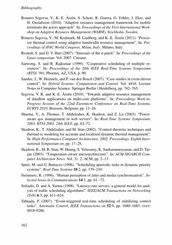
Bibliography
Romero Segovia, V., K.-E. Årzén, S. Schorr, R. Guerra, G. Fohler, J. Eker, andH. Gustafsson (2010). “Adaptive resource management framework for mobileterminals-the actors approach”. In: Proceedings of the First International Work-shop on Adaptive Resource Management (WARM), Stockholm, Sweden.
Romero Segovia, V., M. Kralmark, M. Lindberg, and K.-E. Årzén (2011). “Proces-sor thermal control using adaptive bandwidth resource management”. In: Pro-ceedings of IFAC World Congress, Milan, Italy. Milano, Italy.
Rostedt, S. and D. V. Hart (2007). “Internals of the rt patch”. In: Proceedings of theLinux symposium. Vol. 2007. Citeseer.
Saewong, S. and R. Rajkumar (1999). “Cooperative scheduling of multiple re-sources”. In: Proceedings of the 20th IEEE Real-Time Systems Symposium(RTSS ’99). Phoenix, AZ, USA, p. 90.
Sandee, J., W. Heemels, and P. van den Bosch (2007). “Case studies in event-drivencontrol”. In: Hybrid Systems: Computation and Control. Vol. 4416. LectureNotes in Computer Science. Springer Berlin / Heidelberg, pp. 762–765.
Segovia, V. R. and K.-E. Årzén (2010). “Towards adaptive resource managementof dataflow applications on multi-core platforms”. In: Proceedings Work-in-Progress Session of the 22nd Euromicro Conference on Real-Time Systems,ECRTS 2010. Brussels, Belgium, pp. 13–16.
Sharma, V., A. Thomas, T. Abdelzaher, K. Skadron, and Z. Lu (2003). “Power-aware qos management in web servers”. In: Real-Time Systems Symposium,2003. RTSS 2003. 24th IEEE, pp. 63–72.
Skadron, K., T. Abdelzaher, and M. Stan (2002). “Control-theoretic techniques andthermal-rc modeling for accurate and localized dynamic thermal management”.In: High-Performance Computer Architecture, 2002. Proceedings. Eighth Inter-national Symposium on, pp. 17–28.
Skadron, K., M. R. Stan, W. Huang, S. Velusamy, K. Sankaranarayanan, and D. Tar-jan (2003). “Temperature-aware microarchitecture”. In: ACM SIGARCH Com-puter Architecture News. Vol. 31. 2. ACM, pp. 2–13.
Spuri, M. and G. Buttazzo (1996). “Scheduling aperiodic tasks in dynamic prioritysystems”. Real-Time Systems 10:2, pp. 179–210.
Steinmetz, R. (1996). “Human perception of jitter and media synchronization”. Se-lected Areas in Communications 14:1, pp. 61 –72.
Stiliadis, D. and A. Varma (1998). “Latency-rate servers: a general model for anal-ysis of traffic scheduling algorithms”. IEEE/ACM Transactions on Networking(ToN) 6:5, pp. 611–624.
Tabuada, P. (2007). “Event-triggered real-time scheduling of stabilizing controltasks”. Automatic Control, IEEE Transactions on 52:9, pp. 1680–1685. ISSN:0018-9286.
162

Bibliography
Taymans, W., S. Baker, A. Wingo, R. S. Bultje, and S. Kost (2010). Gstreamerapplication development manual. URL: http://gstreamer.freedesktop.org/data/doc/gstreamer/0.10.30/manual/manual.ps.
Treiber, M., A. Hennecke, and D. Helbing (2000). “Congested traffic states inempirical observations and microscopic simulations”. Phys. Rev. E 62 (2),pp. 1805–1824.
Wang, H., Z. Tian, and Q. Zhang (2010). “Self-tuning price-based congestion con-trol supporting tcp networks”. In: Computer Communications and Networks(ICCCN), 2010 Proceedings of 19th International Conference on, pp. 1–6.
Wolfson, O., B. Xu, and R. M. Tanner (2007). “Mobile peer-to-peer data dissemina-tion with resource constraints”. In: Proceedings of the International Conferenceon Mobile Data Management (2007).
Xenomai (2010). URL: http://www.xenomai.org.Xingang, P, P Goyal, X Guo, and H Vin (1996). “A hierarchical CPU scheduler for
multimedia operating systems”. In: Proceedings of the USENIX 2nd Symposiumon OS Design and Implementation (OSDI ’96), pp. 107–122.
Yaacoub, E., L. Al-Kanj, Z. Dawy, S. Sharafeddine, F. Filali, and A. Abu-Dayya(2012). “A utility minimization approach for energy-aware cooperative contentdistribution with fairness constraints”. Transactions on Emerging Telecommu-nications Technologies 23:4, pp. 378–392. ISSN: 2161-3915.
Zeilinger, M. N., C. N. Jones, D. M. Raimondo, and M. Morari (2009). “Real-timeMPC–stability through robust MPC design”. In: Proceedings of the Joint 48thIEEE Conference on Decision and Control and 28th Chinese Control Confer-enc.
Zhang, L. (1990). “Virtual clock: a new traffic control algorithm for packet switch-ing networks”. In: ACM SIGCOMM Computer Communication Review. Vol. 20.4. ACM, pp. 19–29.
163

AListings
A.1 MIPC
#define MIPC_FAILED -1#define MIPC_SUCCESS 1
#define MIPC_MODE_LOCAL 1#define MIPC_MODE_INET 2
#define MIPC_MAX_MSG_SIZE 1024#define MIPC_PORT_BASE 40000
#define MIPC_PATH "/tmp/mipc/"
struct mipc_msg {int size;void *data;
};
typedef struct mipc_msg mipc_message;typedef int mipc_connection;
int mipc_create_socket(char *path);int mipc_exists(char *path);void* mipc_loop(void *arg);int mipc_connect_server(int addr,
int (*recieve)(mipc_message *msg),int mode);
mipc_connection mipc_connect_client(int addr);mipc_connection mipc_connect_inet_client(char *hostname,
int port);int mipc_send(mipc_connection conn, mipc_message *msg);
164

A.1 MIPC
mipc_message* mipc_new_message(void);void mipc_free_message(mipc_message *msg);
165