From Boolean to Quantitative System Specifications Tom Henzinger EPFL.
78
From Boolean to Quantitative System Specifications Tom Henzinger EPFL
-
date post
21-Dec-2015 -
Category
Documents
-
view
220 -
download
1
Transcript of From Boolean to Quantitative System Specifications Tom Henzinger EPFL.

From Boolean to Quantitative System Specifications
Tom Henzinger EPFL

Outline
1 The Quantitative Agenda
2 Some Basic Open Problems
3 Some Promising Directions

The Boolean Agenda
Property/ Specification
Yes/No
Analysis
Program/ System

The Boolean Agenda
Property/ Specification
Yes/No-perhaps a proof -perhaps some counterexamples -perhaps even a proposed fix
Analysis
Program/ System

The Boolean Agenda
Satisfaction Relation
Property/ Specification
Yes/No-perhaps a proof -perhaps some counterexamples -perhaps even a proposed fix
Structure FormulaProgram/ System

The Boolean Agenda
Program/ System
Property/ Specification
Yes/No-perhaps a proof -perhaps some counterexamples -perhaps even a proposed fix
Analysis
Every request is followed by a grant.
Transition system.

The Boolean Agenda
Quantitative Program/ System
Quantitative Property/
Specification
Yes/No-perhaps a proof -perhaps some counterexamples -perhaps even a proposed fix
Analysis
Every request is followed by a grant within 5 time units.
Timed automaton.

The Boolean Agenda
Quantitative Program/ System
Quantitative Property/
Specification
Yes/No-perhaps a proof -perhaps some counterexamples -perhaps even a proposed fix
Analysis
Every request is followed by a grant within probability 1/2.
Markov process.

The Boolean Agenda
Quantitative Program/ System
Quantitative Property/
Specification
B-perhaps a proof -perhaps some counterexamples -perhaps even a proposed fix
Analysis
Every request is followed by a grant within probability 1/2.
Markov process.

The Quantitative Agenda
Quantitative Program/ System
Quantitative Property/
Specification
R-measure of “fit” between system and spec -could be cost, quality, etc.
Analysis

The Quantitative Agenda
Quantitative Program/ System
Quantitative Property/
Specification
R-measure of “fit” between system and spec -could be cost, quality, etc.
Analysis
Every request is followed by a grant.
The less time between requests and grants, the better.

The Quantitative Agenda
Quantitative Program/ System
Quantitative Property/
Specification
R-measure of “fit” between system and spec -could be cost, quality, etc.
Analysis
Every request is followed by a grant.
The fewer unnecessary grants, the better.
The Quantitative Agenda
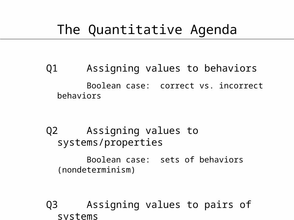
Q1 Assigning values to behaviors
Boolean case: correct vs. incorrect behaviors
Q2 Assigning values to systems/properties
Boolean case: sets of behaviors (nondeterminism)
Q3 Assigning values to pairs of systems
Boolean case: preorders on systems

Q1 Assigning Values To Behaviors
a. Probabilities
b. Resource use
-worst case vs. average case (e.g. response time, QoS) -peak vs. accumulative (e.g. power consumption)
c. Quality measures
-discounting vs. long-run averaging (e.g. reliability)

Q1 Assigning Values To Behaviors
a: ok b: fail
Discounted value (0 < d < 1):
aaaaaaaaaa... 1 aaaaaaab... 1 - d8 aab... 1 - d3 b... 0
Long-run average value:
aaaaaaaaaa... 1 aaabaaabaaab... 1 – ¼
abaabaaab... 1babbabbba... 0

Q2, Q3 Assigning Values To Systems
x: behaviors w: observations A,B: systems
A(w) = supx { val(x) : obs(x) = w } B(w) = expx { val(x) : obs(x) = w }

Q2, Q3 Assigning Values To Systems
x: behaviors w: observations A,B: systems
A(w) = supx { val(x) : obs(x) = w } B(w) = expx { val(x) : obs(x) = w }
diff(A,B) = supw { |A(w) – B(w)| } ? Compositionality: diff(A||B,A’||B) · f(diff(A,A’)) [AFHMS].

Is there a Quantitative Framework with
-an appealing mathematical formulation, -useful expressive power, and -good algorithmic properties?
(Like the boolean theory of -regularity.)

Outline
1 The Quantitative Agenda
2 Some Basic Open Problems
3 Some Promising Directions
Alphabet: = {a,b,c}
Language: L µ L = (a+b)+(a[c[ (a+b)
abaabaaabccccc... 2 Labcabc... L
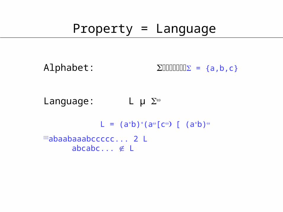
Property = Language
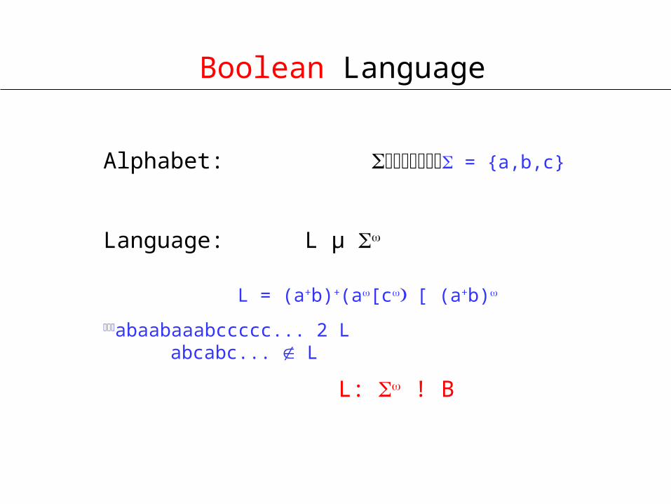
Alphabet: = {a,b,c}
Language: L µ L = (a+b)+(a[c[ (a+b)
abaabaaabccccc... 2 Labcabc... L
L: ! B
Boolean Language

Q states : Q ! labeling q0 2 Q initial state
choices : Q Q transition function
Specification = Automaton
a cb
0
1
0
1
0,1
= {0,1}
A:

Q states : Q ! labeling q0 2 Q initial state
choices : Q Q transition function
Specification = Automaton
a cb
0
1
0
1
0,1
= {0,1} L(A) = (a+b)+(a[c[ (a+b)
A:

Q states : Q ! labeling q0 2 Q initial state
choices : Q Q transition function
Specification = Automaton
a cb
0
1
0
1
0,1
0101111... ! aababccc...
A:
“scheduler” “outcome”

Q states : Q ! labeling q0 2 Q initial state
choices : Q Q transition function
Specification = Automaton
Scheduler: x: Q+ ! S ... set of schedulers
Outcome: f(x) = q0q1q2 ... where 8 i : qi+1 = (qi, x(q0...qi))
Language: L = { (f(x)) : x 2 S }

Satisfaction = Language Inclusion
Given two automata A and B, is L(A) µ L(B)?
i.e. 8 w 2 : L(A)(w) · L(B)(w)

Satisfaction = Language Inclusion
Given two automata A and B, is L(A) µ L(B)?
i.e. 8 w 2 : L(A)(w) · L(B)(w)
For finite automata, PSPACE-complete.

Word: element of Probabilistic Word: probability space on Probabilistic Language: set of probabilistic words
Probabilistic Language
w: ab ! 1/2 aab ! 1/4 aaab ! 1/8
...
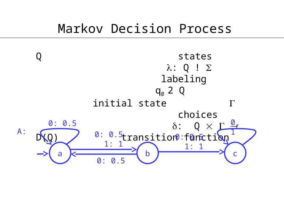
Q states : Q ! labeling q0 2 Q initial state
choices : Q D(Q) transition function
Markov Decision Process
a cb
0: 0.5
0: 0.5 1: 1
0: 0.5
0,1A:
0: 0.5 1: 1

Q states : Q ! labeling q0 2 Q initial state
choices : Q D(Q) transition function
Markov Decision Process
a cb
0: 0.5
0: 0.5 1: 1
0: 0.5
0,1A:
0: 0.5 1: 1
0101111... ! abccc... ! 1/2aabccc... ! 1/4 ...

Q states : Q ! labeling q0 2 Q initial state
choices : Q D(Q) transition function
Markov Decision Process
Pure scheduler: x: Q+ ! Probabilistic scheduler: x: Q+ ! D()

Q states : Q ! labeling q0 2 Q initial state
choices : Q D(Q) transition function
Markov Decision Process
a cb
0: 0.5
0: 0.5 1: 1
0: 0.5
0,1A:
0: 0.5 1: 1
{0: 0.5, 1: 0.5} ! abccc... ! 9/16 aabccc... ! 9/64
...

Probabilistic Language Inclusion
Given two MDPs A and B, is L(A) µ L(B)?

Probabilistic Language Inclusion
Given two MDPs A and B, is L(A) µ L(B)?
?

Probabilistic Language Inclusion
Given two MDPs A and B, is L(A) µ L(B)?
?Open even if specification B is deterministic (i.e. || = 1) and implementation scheduler required to be pure. If both sides are deterministic, then it can be solved in polynomial time (equivalence of Rabin’s probabilistic automata) [Tzeng, DHR].

Language: L: ! B
Quantitative Language: L: ! R
Quantitative Language
L(ab) = 1/2 L(aab) = 1/4 L(aaab) = 1/8 ...

Q states : Q ! labeling q0 2 Q initial state
choices : Q R £ Q transition function
Weighted Automaton
a cb
0; 4
1; 2
0; 0
0,1; 0A:
1; 1

Q states : Q ! labeling q0 2 Q initial state
choices : Q R £ Q transition function
Weighted Automaton
a cb
0; 4
1; 2
0; 0
0,1; 0A:
1; 1
0101111... ! aababccc...; 4 1111111... ! abccc...; 2
Max value:

Q states : Q ! labeling q0 2 Q initial state
choices : Q R £ Q transition function
Weighted Automaton
Outcome: f(x) = q0v1q1v2q2... where 8 i : (vi+1,qi+1) = (qi, x(q0...qi))
Max value: val(q0v1q1v2q2...) = sup{ vi : i ¸ 1 }

Q states : Q ! labeling q0 2 Q initial state
choices : Q R £ Q transition function
Weighted Automaton
Outcome: f(x) = q0v1q1v2q2... where 8 i : (vi+1,qi+1) = (qi, x(q0...qi))
Max value: val(q0v1q1v2q2...) = sup{ vi : i ¸ 1 }
q-Language: L(w) = sup{ val(f(x)) : x 2 S s.t. (f(x)) = w }

Different Value Functions
Max value: val(q0v1q1v2q2...) = sup{ vi : i ¸ 1 } (only 0 and 1 costs: finite automaton)
Limsup value: val = limn!1 sup{ vi : i ¸ n } (only 0 and 1 costs: Buechi automaton)

Different Value Functions
Max value: val(q0v1q1v2q2...) = sup{ vi : i ¸ 1 } (only 0 and 1 costs: finite automaton)
Limsup value: val = limn!1 sup{ vi : i ¸ n } (only 0 and 1 costs: Buechi automaton)
Limavg value: val = limn!1 1/n ¢ 1·i·n vi

Different Value Functions
Max value: val(q0v1q1v2q2...) = sup{ vi : i ¸ 1 } (only 0 and 1 costs: finite automaton)
Limsup value: val = limn!1 sup{ vi : i ¸ n } (only 0 and 1 costs: Buechi automaton)
Limavg value: val = limn!1 1/n ¢ 1·i·n vi
Discounted: val = i¸ 1 di ¢ vi for some 0<d<1

Weighted Automaton
a cb
0; 4
1; 2
0; 0
0,1; 0A:
1; 1
01010101... ! aabababab...; 2 11111111... ! abccc...; 0
Limsup value:
01010101... ! aabababab...; 1 11111111... ! abccc...; 0
Limavg value:
01010101... ! aabababab...; 2.66... 11111111... ! abccc...; 1.25
Discounted: (d = 0.5)

Quantitative Language Inclusion
Given two weighted automata A and B, is 8 w 2 : L(A)(w) · L(B)(w) ?

Quantitative Language Inclusion
Given two weighted automata A and B, is 8 w 2 : L(A)(w) · L(B)(w) ?
For max and limsup values: PSPACE. For limavg and discounted values: Open.

Quantitative Language Inclusion
Given two weighted automata A and B, is 8 w 2 : L(A)(w) · L(B)(w) ?
For max and limsup values: PSPACE. For limavg and discounted values: Open.
If specification B is deterministic, then it can be solved in polynomial time [CDH].

Quantitative Simulation
a
1
b1
1
1
b
2
a2
0
0
b
0
a0
2
2
a
2
0
·
A not simulated by B.
Simulation game solvable in P for max, and in NP Å coNP for limsup, limavg, discounted [CDH].
A: B:
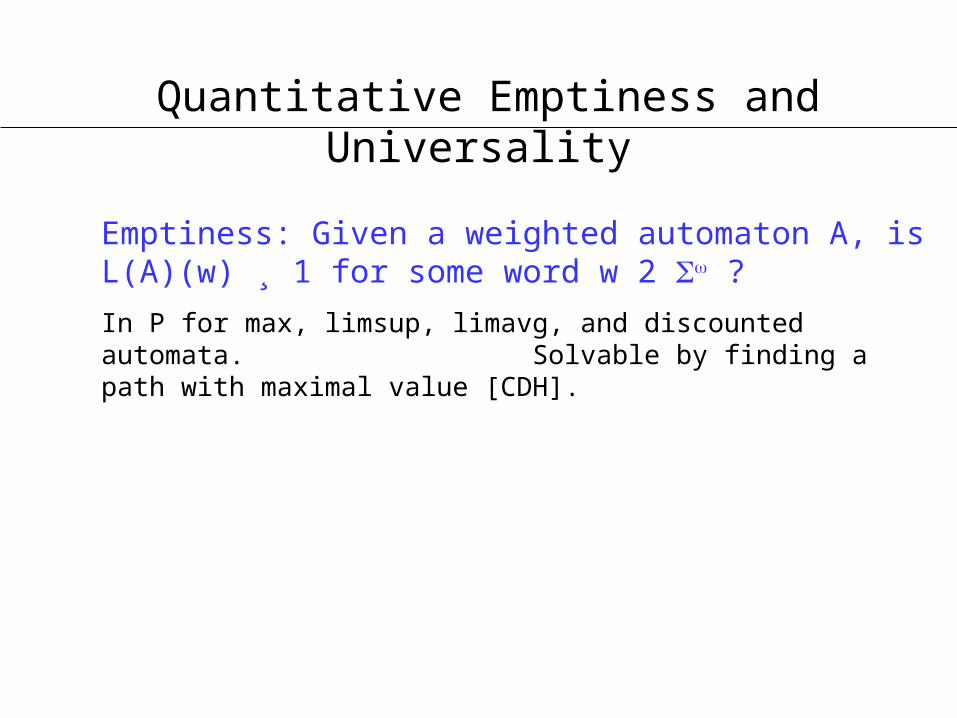
Quantitative Emptiness and Universality
Emptiness: Given a weighted automaton A, is L(A)(w) ¸ 1 for some word w 2 ?
In P for max, limsup, limavg, and discounted automata. Solvable by finding a path with maximal value [CDH].

Quantitative Emptiness and Universality
Emptiness: Given a weighted automaton A, is L(A)(w) ¸ 1 for some word w 2 ?
In P for max, limsup, limavg, and discounted automata. Solvable by finding a path with maximal value [CDH].
Universality: Given a weighted automaton A, is L(A)(w) ¸ 1 for all words w 2 ?
As hard as language inclusion.

Quantitative Expressiveness
[CDH CSL08, LICS09]

Quantitative Expressiveness
ba,b
0 1
E.g. limavg automata not determinizable:
*b expressible by a nondeterministic limavg automaton.
*b not expressible by a deterministic limavg automaton.
Every b-cycle would need weight 1.Consider wn = (abn).Then val(wn)=1 for sufficiently large n, but wn*b.
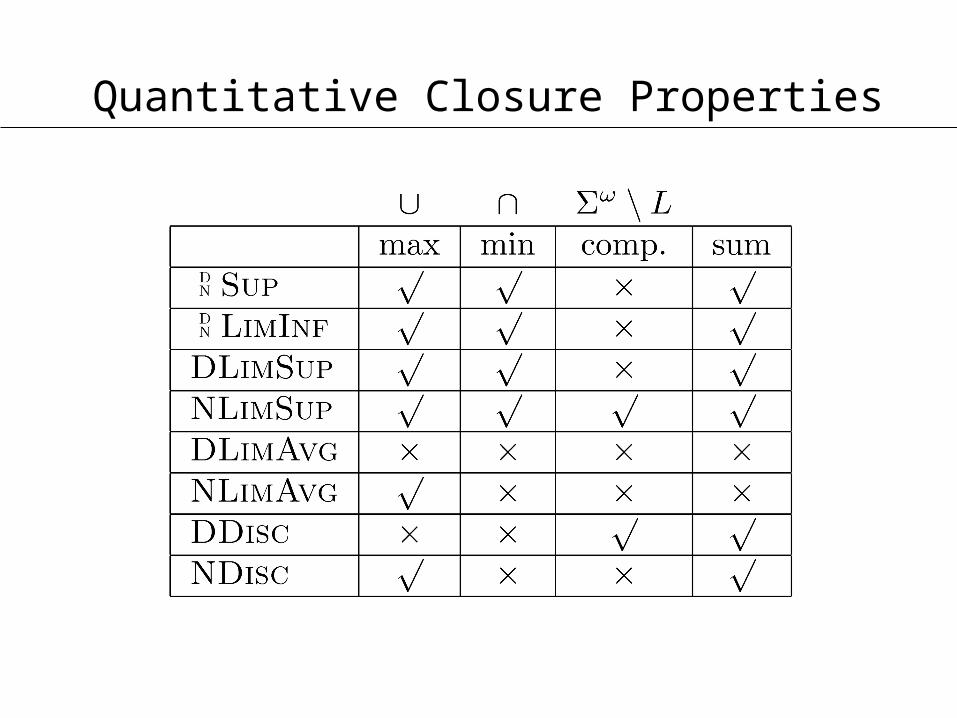
Quantitative Closure Properties
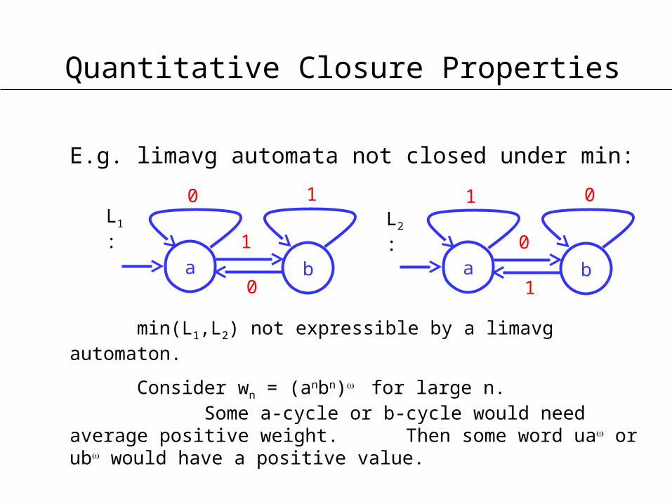
Quantitative Closure Properties
a
0
b0
1
1
a
1
b1
0
0
E.g. limavg automata not closed under min:
min(L1,L2) not expressible by a limavg automaton.
Consider wn = (anbn) for large n.Some a-cycle or b-cycle would need average positive weight.Then some word ua or ub would have a positive value.
L1: L2:

Outline
1 The Quantitative Agenda
2 Some Basic Open Problems
3 Some Promising Directions

The Boolean Agenda
Specification
Yes/No
Analysis
System

The Boolean Agenda
Specification
Correct System
Synthesis

The Boolean Agenda
Regular Automaton
Correct System = Winning Strategy
Graph Game with Regular Objective

3.1 Quantitative Synthesis
Optimal System
Synthesis
Quantitative Specification
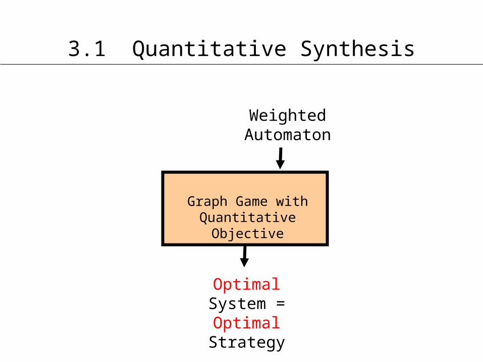
3.1 Quantitative Synthesis
Optimal System = Optimal Strategy
Weighted Automaton
Graph Game with Quantitative Objective

3.1 Quantitative Synthesis
Graph Game with Quantitative Objective
Weighted Automaton
Optimal System = Optimal Strategy
-positional vs. finite-memory vs. unrestricted strategies
-optimal vs. -optimal strategies
Games for Quantitative Synthesis
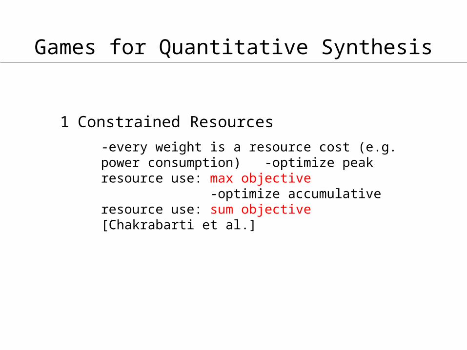
1 Constrained Resources
-every weight is a resource cost (e.g. power consumption) -optimize peak resource use: max objective -optimize accumulative resource use: sum objective [Chakrabarti et al.]

Games for Quantitative Synthesis
1 Constrained Resources
2 Preference between Different Implementations
-boolean spec, but certain implementations preferred-formalized using lexicographic objectives
[Jobstmann et al.]
h f, g1, ... gn i
boolean objective quantitative objectives
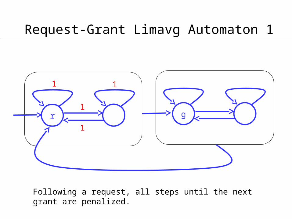
Request-Grant Limavg Automaton 1
r g
1
1
11
Following a request, all steps until the next grant are penalized.

Request-Grant Limavg Automaton 2
r g
1
1
Following a request, all repeated grants are penalized.

3.2 Robust Systems
1 Robustness as Mathematical Continuity:
-small input changes should cause small output changes -only possible in a quantitative framework
8 >0. 9 >0. input-change · ) output-change ·

In general programs are not continuous. But they can less continuous:
read sensor value x; if x · c then y = f1(x)
else y = f2(x);
f1
f2
c

In general programs are not continuous. But they can less continuous:
read sensor value x; if x · c then y = f1(x)
else y = f2(x);
Or more continuous:
if x · c - then y = f1(x); if x ¸ c + then y = f2(x)
else y = (f2(c+)-f1(c-))(x-c+)/2 + f1(c-);
[Majumdar et at., Gulwani et al.]
f1
f2
c

3.2 Robust Systems
1 Robustness as Mathematical Continuity:
-small input changes should cause small output changes -only possible in a quantitative framework
8 >0. 9 >0. input-change · ) output-change ·
Example of a Robustness Theorem [AHM]:
If discountedBisimilarity(A,B) > 1 - , then 8w : |A(w) – B(w)| < f().
3.2 Robust Systems
1 Robustness as Mathematical Continuity:
-small input changes should cause small output changes -only possible in a quantitative framework
2 Robustness w.r.t. Faulty Assumptions:
-environment may violate assumptions -few environment mistakes should cause few system
mistakes -ratio of system to environment mistakes as
quantitative quality measure
[Greimel et al.]

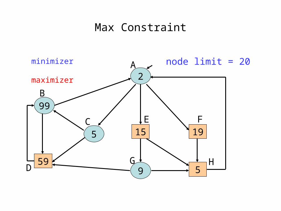
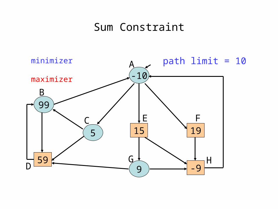
3.3 Resource Interfaces
-Component interfaces expose resource requirements (e.g. time, memory, power).
-Interfaces are compatible if their combined requirements do not exceed the available resources.
-If the requirements are dynamic, then compatibility can be solved as a graph game with quantitative objectives.
[Chakrabarti et al.]
2
99
5
9 5
15 19
59
A
B
C
D
E F
G H
node limit = 20
Max Constraint
minimizer maximizer

2
99
5
9 5
15 19
59
A
B
C
D
E F
G H
node limit = 20
Max Constraint
minimizer maximizer
-10
99
5
9 -9
15 19
59
A
B
C
D
E F
G H
path limit = 10
Sum Constraint
minimizer maximizer

-10
99
5
9 -9
15 19
59
A
B
C
D
E F
G H
path limit = 10
Sum Constraint
minimizer maximizer

3.4 System Reliability
-assuming x% of periodic input values are valid, y% of periodic output values should be valid
-hardware faulty, but can be replicated
-compiler ensures specified reliability through replication
[Ghosal et al.]
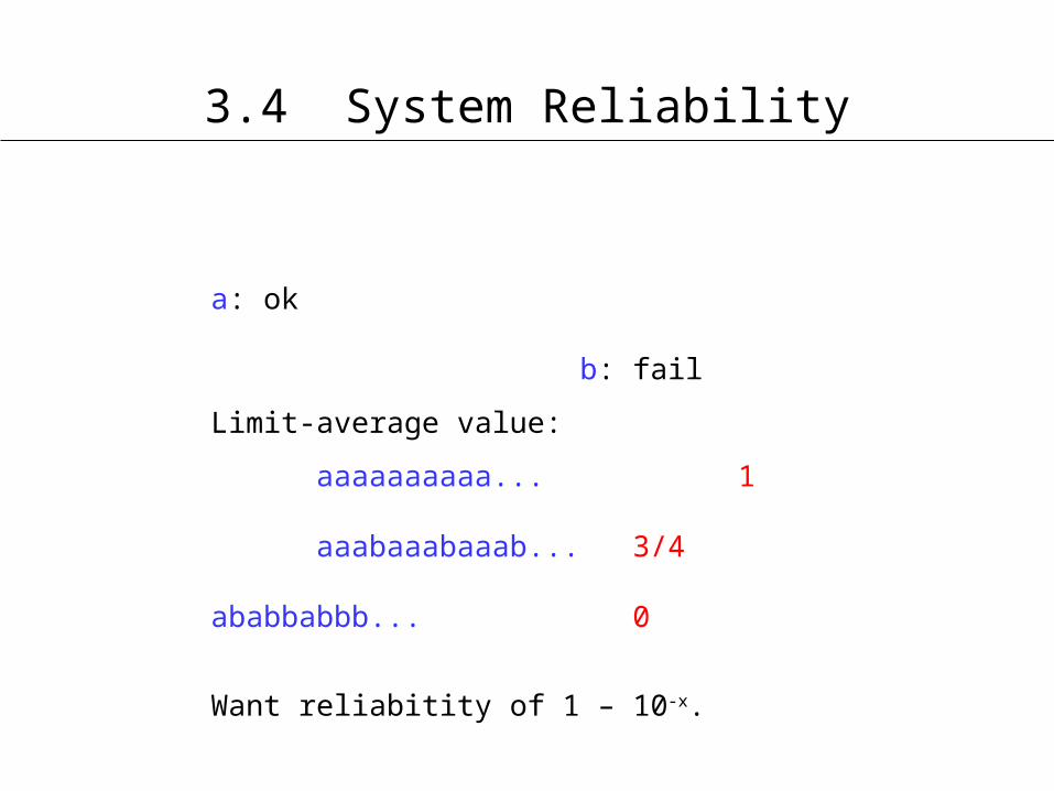
3.4 System Reliability
a: ok b: fail
Limit-average value:
aaaaaaaaaa... 1 aaabaaabaaab... 3/4 ababbabbb... 0
Want reliabitity of 1 – 10-x.

Conclusions
-“Quantitative” is more than “timed” and “probabilistic.”
-We need to move from boolean correctness criteria to quantitative system preference metrics.
-We have interesting point solutions, but no convincing overall framework.