From “Statistical Mechanics Made Simple” by D. C. Mattis...
50
1 Core text: Statistical Physics by F. Mandl, various editions 'University Physics' by Young&Freedman, 11 th Ed. 17. Temperature and Heat 18. Thermal Properties of Matter 19. The First Law of Thermodynamics 20. The Second Law of Thermodynamics Supplementary texts: Introductory Statistical Mechanics by R. Bowley and M. Sánchez, various editions. Heat and Thermodynamics by M. W. Zemansky & R. H. Dittman, various editions. also any other good textbook such as Thermal Physics by P. C. Riedi, various editions. PHY2023 Thermal Physics - Misha Portnoi Rm. 212 From “Statistical Mechanics Made Simple” by D. C. Mattis (World Scientific, 2010) Despite the lack of a reliable atomic theory of matter, the science of Thermodynamics flourished in the 19th century. Among the famous thinkers it attracted, one notes William Thomson (Lord Kelvin) after whom the temperature scale is named, and James Clerk Maxwell. The latter's many contributions include the "distribution function" and some very useful "differential relations" among thermodynamic quantities (as distinguished from his even more famous "equations" in electro-dynamics). The Maxwell relations set the stage for our present view of thermodynamics as a science based on function theory while grounded in experimental observations. From “Statistical Mechanics Made Simple” by D. C. Mattis (World Scientific, 2010) The kinetic theory of gases came to be the next conceptual step. Among pioneers in this discipline one counts several unrecognized geniuses, such as J. J. Waterston who - thanks to Lord Rayleigh - received posthumous honours from the very same Royal Society that had steadfastly refused to publish his works during his lifetime. Ludwig Boltzmann committed suicide on September 5, 1906, depressed by the utter rejection of his atomistic theory by such colleagues as Mach and Ostwald. Paul Ehrenfest, another great innovator, died by his own hand in 1933. Among 20th century scientists in this field, a sizable number have met equally untimely ends. So “now it is our turn to study statistical mechanics” [D.H.Goodstein, States of Matter]
Transcript of From “Statistical Mechanics Made Simple” by D. C. Mattis...

1
Core text: Statistical Physics by F. Mandl, various editions'University Physics' by Young&Freedman, 11th Ed. 17. Temperature and Heat 18. Thermal Properties of Matter 19. The First Law of Thermodynamics 20. The Second Law of Thermodynamics
Supplementary texts:Introductory Statistical Mechanics by R. Bowley and M. Sánchez, various editions.
Heat and Thermodynamics by M. W. Zemansky & R. H. Dittman, various editions. also any other good textbook such asThermal Physics by
P. C. Riedi, various editions.
PHY2023 Thermal Physics - Misha Portnoi Rm. 212
From “Statistical Mechanics Made Simple”
by D. C. Mattis (World Scientific, 2010) Despite the lack of a reliable atomic theory of matter, the science of Thermodynamics flourished in the 19th century. Among the famous thinkers it attracted, one notes William Thomson (Lord Kelvin) after whom the temperature scale is named, and James Clerk Maxwell. The latter's many contributions include the "distribution function" and some very useful "differential relations" among thermodynamic quantities (as distinguished from his even more famous "equations" in electro-dynamics). The Maxwell relations set the stage for our present view of thermodynamics as a sciencebased on function theory while grounded in experimental observations.
From “Statistical Mechanics Made Simple”
by D. C. Mattis (World Scientific, 2010) The kinetic theory of gases came to be the next conceptual step. Among pioneers in this discipline one counts several unrecognized geniuses, such as J. J. Waterston who - thanks to Lord Rayleigh - received posthumous honours from the very same Royal Society that had steadfastly refused to publish his works during his lifetime. Ludwig Boltzmann committed suicide on September 5, 1906, depressed by the utter rejection of his atomistic theory by such colleagues as Mach and Ostwald. Paul Ehrenfest, another great innovator, died by his own hand in 1933. Among 20th century scientists in this field, a sizable number have met equally untimely ends. So “now it is our turnto study statistical mechanics” [D.H.Goodstein, States of Matter]
2
Temperature and Heat
ThermodynamicsStatistical Mechanics
Macroscopicdescription of a
'system'
Microscopicdescription of a
'system'
Statistical Thermodynamics
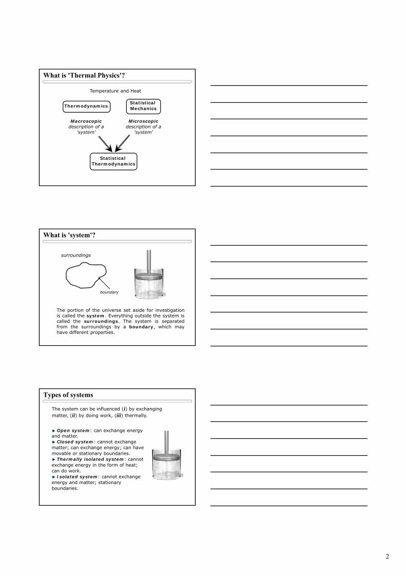
What is 'Thermal Physics'?
boundary
surroundings
The portion of the universe set aside for investigationis called the system. Everything outside the system iscalled the surroundings. The system is separatedfrom the surroundings by a boundary, which mayhave different properties.
What is 'system'?
The system can be influenced (i) by exchanging matter, (ii) by doing work, (iii) thermally.
Open system: can exchange energy and matter.
Closed system: cannot exchange matter; can exchange energy; can have movable or stationary boundaries.
Thermally isolated system: cannot exchange energy in the form of heat; can do work.
Isolated system: cannot exchange energy and matter; stationary boundaries.
Types of systems

3
The system is characterised by:
chemical composition volumepressuretemperaturedensity
The macroscopic quantities that are usedto specify the state of the system arecalled the state variables; their valuesdepend only on the condition or the stateof the system.
The Macroscopic View (human scale or larger)
The system is considered asconsisting of a large numberof particles, existing in a setof energy states.
Probabilistic analysis.
Statistical Mechanics
The Microscopic View (molecular scale or smaller)
If the same system is considered, the two approaches must lead to the same conclusion!
How? Macroscopic parameters
Microscopic parameters averaged over time
e.g. PressureAverage rate of change in momentum due to all molecular collisions on a unit area
Macroscopic vs. Microscopic

4
AState SA
How an intuitive concept can be developed analytically?
Open systems Closed systems Thermally isolated systems Isolated systems
System & Surroundings
State Variables
Boundary: in general, it may exchange matter and/or energy
What is Temperature?
Definition: An equilibrium state is one in which all the state variables are uniform throughout the system and do not change in time.
AState SA
When a system suffers a change in its surroundings, it usually is seen to undergo change. After a time, the system will be found to reach a state where no further change takes place. The
system has reached thermodynamic equilibrium.
Similarly, if two systems are placed in thermal contact, generallychanges will occur in both. When there is no longer any change,the two systems are said to be in thermal equilibrium. Theequilibrium state is determined by the equilibrium values of thestate variables.
Thermodynamic Equilibrium and Thermal Equilibrium
AState SA
BState SB
boundary
The equilibrium state depends on the nature of the boundary!
Adiabatic boundary: perfectly insulating.
Any SA can coexist with any SB
Thermal Equilibrium: SA and SB are constant, but not necessary equal.
Diathermic boundary: perfectly conducting.
Change in SA leads to change in SB
Thermal Equilibrium

5
A B
C
A B
C
A and B are insulated from each other, but are both in thermal equilibrium with C.
What will happen, if A and Bare brought into contact via a diathermic wall?
Result: no change in the states of A and B.
This means that A and B are in thermal equilibrium: the twosystems are found in such states that, if the two wereconnected through a diathermic wall, the combined systemwould be in thermal equilibrium.
adiabatic
adiabaticdiathermic
diathermic
The experiment
Two systems in thermal equilibrium with a third one are in thermal equilibrium with each other.
(Fowler & Guggenheim 1939)
[First Law – Helmholz 1847
Second Law – Carnot 1824]
Is this obvious?
The Zeroth Law of Thermodynamics
All systems in thermal equilibrium with each other possess a common property which we call the temperature.
The temperature is that property that determines whether a system is in thermal equilibrium with other systems.
Two systems are in thermal equilibrium if and only if they have the same temperature.
Temperature

6
In any process where heat Q is added to the system and
work W is done by the system, the net energy transfer,
Q W, is equal to the change, U, in the internal energy of the system.
Qincrease internal energy
work on surroundings
The First Law of Thermodynamics
The First Law of Thermodynamics
Sign convention: In most statistical physics textbooks W is the work done on the system. Work W is positive if it is done on the system, similar to Q, which is positive if heat is added to the system.
In Joule’s paddle-wheel experiment the work of gravity was indeed done onthe system!
Thus
The First Law states:
Conservation of energy in thermodynamic systems
dU is an exact differential.U is a function of the state of the system only.
depends only on the initial and end states and not on the path between them
Internal energy depends only on the state of the system, i.e. its change is path-independent
The First Law of Thermodynamics

7
Exact differentials
where the notation means differentiating with respect to y keeping xconstant. Such derivatives are called partial derivatives.
In general, is an exactdifferential and, correspondingly, F(x,y) does not depend on the path only if
The First Law does not explain:
The First Law: A perpetual motion machine of first kind is impossible.
Ease of converting work to heat but not vice versa.
The First Law of Thermodynamics
Systems naturally tend to a state of disorder, not order.
Heat only flows DOWN a temperature gradient.
T1 > T2 T2 T TX
XGas Vacuum Gas Gas
Although there would be no violation of the First Law, the reverse processes do not happen. Therefore, there must be a principle, dictating the direction of the processes in isolated systems:
the Second Law
The Second Law
8
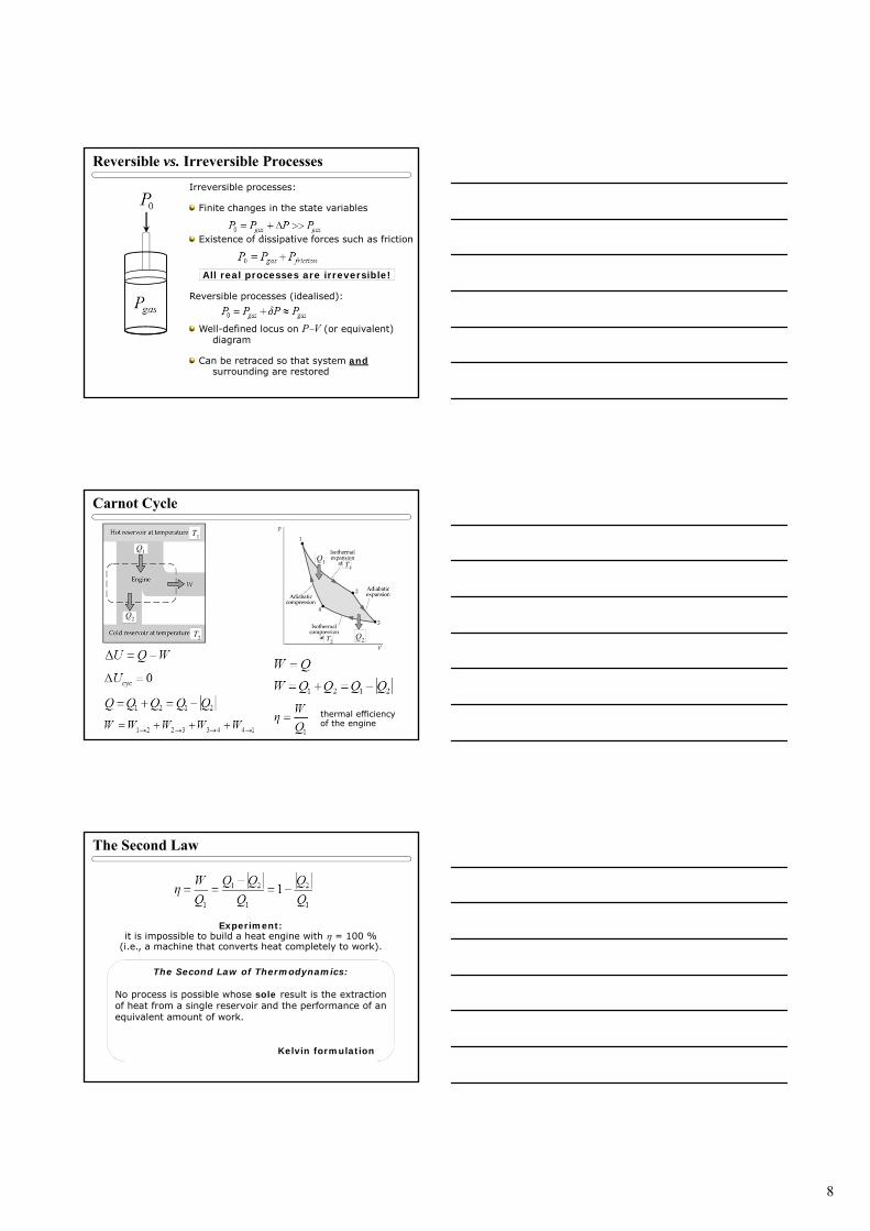
Irreversible processes:
Finite changes in the state variables
Existence of dissipative forces such as friction
All real processes are irreversible!
Reversible processes (idealised):
Well-defined locus on PV (or equivalent) diagram
Can be retraced so that system andsurrounding are restored
Reversible vs. Irreversible Processes
Q1
Q2
Q1
Q2
T1
T2
T1
T2
thermal efficiency of the engine
Carnot Cycle
Experiment:it is impossible to build a heat engine with = 100 %
(i.e., a machine that converts heat completely to work).
The Second Law of Thermodynamics:
No process is possible whose sole result is the extractionof heat from a single reservoir and the performance of anequivalent amount of work.
Kelvin formulation
The Second Law

9
Q1
Q2
T1
T2
Working substance: ideal gas
Thermal Efficiency of the Carnot Cycle
Q1
Q2
T1
T2
Thermal Efficiency of the Carnot Cycle
Q1
Q2
coefficient of performance
Refrigerators extract heat from acolder reservoir and transfer it to ahotter reservoir. Experience showsthat this always requires work.
The Second Law of Thermodynamics:
No process is possible whose sole result is the removalof heat from a reservoir at one temperature and theabsorption of an equal quantity of heat by a reservoir ata higher temperature.
Clausius formulation
for heat pumps
T1
T2
Carnot Cycle as a refrigerator

10
No engine can be more efficient than a Carnot engine operating between the same two
temperatures.
Q1
W
Carnot engine
Thermal Efficiency of the Carnot Cycle
Independent of working substance
Depends only on reservoir temperatures T1 and T2
Maximum possible efficiency of any heat engine
Equal to the efficiency of any other reversible heat engine
Note that = 1 when T2 = 0.
Therefore, the Second Law forbids attainment of the absolute zero.
Thermal Efficiency of the Carnot Cycle
Q1
Q2
T1
T2
Consider any reversible cyclic process. It can be approximated by an infinite number of Carnot cycles.
By summing up Q/T for each of them we obtain:
for any reversible cyclic process.
Entropy

11
for any reversible cyclic process.
This means that is an exact differential.
dS is an exact differential, therefore the entropy S is a function of state.
S entropy
The change in entropy S between two states is determined solely by the initial and final equilibrium
states and not by the path between them.
Reversible only!
For an infinitesimal reversible change:
Entropy
Remember that the reversible Carnot engine has a maximalthermal efficiency, equal to the efficiency of any otherreversible heat engine.
Compare a reversible (R) and an irreversible (I) heat engine:
Compare with
irreversible reversible
Entropy and irreversible processes
P
V
1
2
(I)
(R)
For an infinitesimal process:
(note that the equality applies only if the process is reversible)
Entropy and irreversible processes

12
For a system which is thermally isolated (or completely isolated) Q = 0:
The entropy of a (thermally) isolated system cannot decrease!
Entropy distinguishes between reversible and irreversible processes.
Helps determine the direction of natural processes and equilibrium configuration of a (thermally) isolated system: maximal entropy.
Provides a natural direction to the time sequence of natural events.
Entropy and irreversible processes
The Clausius inequality
In a (thermally) isolated system, spontaneous processes proceed in the direction of increasing entropy.
Consider processes like irreversible heat flow or free expansion of a gas. They result in increased disorder.
Example: Reversible (quasistatic) isothermal expansion of an ideal gas:
is a measure of the increase in disorder
Entropy and disorder
Microscopically, the entropy of a system is a measure of the degree of molecular disorder existing in the system
(much more on this later in this module):
is the thermodynamic probability
Therefore, in a (thermally) isolated system, only processes leading to greater disorder (or no change of order) will be possible, since the entropy must increase
or remain constant, .
Entropy and disorder

13
always reversible reversible
Here all the variables are functions of state, so that all the differentials are exact. Therefore, it is true for all processes.
where
More generally
The Fundamental Thermodynamic Relationship
1) A nuclear power station is designed to generate 1000 MW of electrical power. To do this it maintains a reservoir of superheated steam at a temperature of 400 K. Waste heat from the reactor is transferred by a heat exchanger to circulating sea water at 300 K. What is the minimum possible rate of nuclear energy generation needed?
Exercises
2) You are asked to design a refrigerated warehouse to maintain perishable food at a temperature of 5 C in an external environment of up to 30 C. The size of the warehouse and its degree of thermal insulation mean that the refrigeration plant must extract heat at a rate of 1000 KW. As a first step you must supply the local electricity company with an estimate for the likely electrical consumption of the proposed warehouse. What value would you suggest as a working minimum?
Exercises

14
3) One mole of ideal gas is maintained at a temperature T.
a) What is the minimum work needed to reduce its volume by a factor of e (=2.718…) ?
b) What is the entropy loss of the gas during this process?
4) 1 kg of water at 20C is placed in thermal contact with a heat reservoir at 80C. What is the entropy change of the total system (water plus reservoir) when equilibrium has been re-established?
Exercises
5) Demonstrate that the entropy change for n moles of ideal gas can also be written as
where T1, P1 and T2, P2 are the initial and final temperatures and pressures respectively and CP is the heat capacity at constant pressure.
Exercises
6) Consider two identical bodies with heat capacity Cinitially at different temperatures T1 and T2. Show that the process of reaching thermal equilibrium necessarily involves a total increase in entropy.[See Supplement 1 on ELE]
Exercises

15
Preamble: distribution functions
ni: number of students who received mark si
ni(si) and fi(si): distribution functions
1. Discrete distributions
14.2 Mark
Statistical Mechanics: an introduction
smp = 16
2. Continuous distributionsf(h)dh: the probability of a person having a height between h and h+dh
f(h): distribution function
dN = Nf(h)dh: number of people with height between h and h+dh
Statistical Mechanics: an introduction
What is the distribution of molecular speeds about average?
Expect:
Mean vx = 0 (no convection).
No. of molecules with vx = No. of molecules with vx(even distribution function).
No. of molecules with vx → ±∞ is negligible.
The Maxwell-Boltzmann distribution

16
Let f(vx) is the velocity distribution function.
Then the probability a molecule will have velocity between vx and (vx + dvx) is:
The number of molecules with velocity between vx and (vx + dvx) is:
as required
The Maxwell-Boltzmann distribution
Guess that velocity distribution is Gaussian (normal distribution)
[can be derived using SM or from symmetry arguments]:
vx vx 0
A
Satisfies our three expectations.
A determines the height (normalisation)
B is inversely related to the width
The Maxwell velocity distribution
1. Normalisation (determines A)
Remember that
Therefore
2. Physical meaning of B
Calculate :
The Maxwell velocity distribution

17
For the distribution function we have:
The Maxwell velocity distribution
In 3 dimensionsThe probability a molecule will have velocity between vx and (vx + dvx), vy and (vy + dvy), vz and (vz + dvz)
The Maxwell velocity distribution
What is the probability a molecule having speed between v and v + dv?
(remember that )
The Maxwell-Boltzmann speed distribution function

18
As T increases the curve flattens and the peak moves towards higher speeds.
Effect of temperature
1. Mean (average) speed
2. Root Mean Square (rms) speed
Molecular speeds
3. Most probable speed
Occurs at
Molecular speeds

19
The Maxwell-Boltzmann energy distribution function
Starting from
find the distribution function F(E) for the energy by calculating the probability for a molecule to have energy between E and E + dE:
where
Answer:
Examples
The Maxwell-Boltzmann energy distribution function
We can exploit the 1:1 correspondence between and v to reformulate the speed distribution as a kinetic energy distribution :
v
v0
0
v0+dv
0+d
The Maxwell-Boltzmann energy distribution function
Since a speed between v0 and v0+dvimplies an energy between 0 and 0+d, with ,the probability of obtaining a speedbetween v0 and v0+dv equals probabilityof obtaining an energy between 0 and 0+d. hence, with

20
The Maxwell-Boltzmann energy distribution function
Exercise: What happens in a 2D case?
The Maxwell-Boltzmann energy distribution function
Example of the Boltzmann factor
Consider a mass of isothermal ideal gas, at temperature T. For a thin slab of gas at height z0, thickness z and cross-sectional area A to not fall under gravity requires :
z=z0
z=z0+z
p(z0+z).A
p(z0).A
Hydrostatic equilibrium:-

21
Example of the Boltzmann factor
Expanding p(z) in a Taylor series:
In the limit that the slab thickness z0,
Hence,
With mA being the mass of one gas atom and nbeing the number density of gas atoms.
Example of the Boltzmann factor
Ideal gas equation of state:
hence
Hence n(z), (z) and p(z) all fall exponentially with height.
Here mAgz is the gravitational potential energy of a gas atom at height z. Since n(z) probability of finding a gas atom at height z, suggests that the probability of finding a gas atom in an “energy level” of value (z) is proportional to
- Boltzmann factor
Example of the Boltzmann factor
The Boltzmann factor is of universal validity; whenever an ensemble of classical particles are in equilibrium at temperature T, the probability of an energy level of value (z) being “occupied” by a particle of the ensemble varies as the negative exponential of (z)/kBT.
Energy
Probability of a particle possessing this energy

22
Mathematical detour
Plot (sketch)
Consider
Find A from the “normalisation” condition:
(a)
(b)
Mathematical detour
Example of Boltzmann energy sharing
7 identical, but distinguishable systems, each with quantized energy levels 0, 1, 2, 3 … We have a total energy of 7 to share amongst the systems. Labeling the systems A…G, some possible arrangements are :-
Note that the first two, distinct, arrangements nevertheless correspond to an identical macroscopicenergy sharing arrangement (macrostate ‘a’ in the table below).

23
Example of Boltzmann energy sharing
Denoting the number of systems in energy level i as ni, then , the number of possible microstates corresponding to this macrostate is given by
or in general
Since the ni’s must satisfy the constraints
and with N the total number of systems
and U the total shared energy, we can complete the table of for each macrostate
Example of Boltzmann energy sharing
Example of Boltzmann energy sharing
Note that, if one of the 1,716 distinct microstates were chosen at random, macrostate ‘j’ would occur with a probability of 420/1716 i.e. 24%. This is the most probable macrostate, and distributes the available energy roughly as a negative exponential function:
i.e. the relative occupancy of an energy level falls exponentially as the energy of that level increases. This pattern becomes clearer as the number of systems and the shared energy are increased.

24
Example of Boltzmann energy sharing
In total, there are 1,716 possible ways to share 7amongst 7 identical systems. To calculate this directly, consider 7 distinguishable heaps A, B, C… G. How many ways can we distribute 7 identical bricks among these? One possibility is
Example of Boltzmann energy sharing
Equivalent problem. Consider a pile of 7 bricks and 6 partitions (all indistinguishable).
If we draw objects (bricks or partitions) at random, each distinct sequence of bricks and partitions corresponds to exactly one possible distribution of 7 bricks amongst 7 heaps e.g. the possible arrangement noted above corresponds to the sequence
Example of Boltzmann energy sharing
| | | | | |
If bricks and partitions are indistinguishable, number of ways equals
Hence in general, we can distribute Npackets of energy over k systems in
ways.

25
The fundamental postulates of statistical mechanics
1. An ensemble of identical but distinguishable systems can be described completely by specifying its “microstate”. The microstate is the most detailed description of an ensemble that can be provided. For an ideal gas of N particles in a container, it involves specifying 6Nco-ordinates, the position and velocity of all N particles. For the example of Boltzmann energy sharing, it involves specifying the energy level occupied by each individual system.
The fundamental postulates of statistical mechanics
2. Physically we observe only a corresponding “macrostate”, specified in terms of macroscopically observable quantities. A macrostate for an ideal gas is specified fully by a few observable quantities such as pressure, temperature, volume, entropy etc. For the example of Boltzmann energy sharing, a macrostate is specified fully by the occupancies of the various energy levels e.g. [0,7,0,0,0,0,0,0…] is a macrostate of equal energy sharing.
The fundamental postulates of statistical mechanics
3. If we observe an ensemble over time, random perturbations ensure that all accessible microstates will occur with equal probability. Hence probability of a macrostate occurring =
4. The macrostate with the highest probability of occurrence corresponds to the equilibrium state.

26
Boltzmann distribution
Maximise
subject to the constraints
using Lagrange Undetermined Multipliers (see supplementary sheet).
Solution: (with undetermined)
Assigning
Boltzmann distribution
Boltzmann distributionNB ni / N is the probability that a state of energy i is occupied by a member of an ensemble which is in thermal equilibrium at temperature T.
Examples
Ensemble of N gas atoms. Outer electron can reside in a “ground-state” energy level, or in an excited state, 1 eV above this. At 1000 K, what fraction of atoms lie in the excited state, relative to the ground-state?
Boltzmann distribution:
ni is no. of systems occupying a state of energy i, when ensemble of N such systems is in thermal equilibrium at temp T. For a 2-level system, energies 1, 2, relative occupancy of these levels is given by

27
Examples
with
Useful “rule of thumb”: At room temperature (300K) the thermal energy kBT is 25 meV
Examples
Hence at 1000 K the thermal energy is 25 meV1000/300.
n2/n1 = exp(–1/(2510–3 10/3)) = exp(-12) = 610–6
Cool the gas to 300 K:-
n2/n1 = 610–6
n2/n1 = exp(–1/(25*10–3)) = exp(–40) = 410–18
n2/n1 = 410–18
Very strong T-dependence!
Examples
Ensemble of protons, magnetic moment , in external magnetic field B. Magnetostatic potential energy = +Bif proton spin anti-parallel to field, –B if proton spin parallel to field.
Simple 2-level system:
B
1 = +B
0 = –B
Proton spin vector
In equilibrium, what is the net imbalance between spin “aligned” (n) and spin “anti-aligned” (n) protons (i.e. what is the fractional magnetization) at room temperature?

28
Examples
Proton = 1.4110–26 JT–1. B = 1 T (typically), T = 300 K. Hence 2B = 2.8210–26 J.
kBT = 1.3810–23300 J = 4.1410–21 J.
Since 2B << kBT :
Examples
Hence at 300K and 1 T, the net imbalance of proton spins is 1.4110–26 / 4.1410–21 J
= 3.410–6
i.e. a very small imbalance.
Degeneracy
More than one ‘state’ can correspond to the same ‘energy level’.‘State’: the fullest description of a system allowed by quantum mechanics. A full set of ‘quantum numbers’must be specified, specifying e.g. the energy, orbital angular momentum and spin of the system. ‘Energy level’:- a quantized energy value that can be possessed by the system. Specified using a single quantum number (the ‘principal’ quantum number).
E.g., electron of mass me in a 1-D infinite potential well of width L
The integer n (=1, 2, 3…) labels the energy levels and is the principle quantum number.

29
Degeneracy
To fully specify the state of an electron in the well we must specify two quantum numbers nand s (s = –½ or ½). s is the “spin” quantum number and specifies whether the electron spin is found to be “up” or “down” if measured relative to a given direction in space. In the absence of an external electromagnetic field, the energies of state (n, –½) and (n, ½) are identical. Thus energy level n is said to be two-fold degenerate (or to have a degeneracy factor g equal to 2) in this example.
Degeneracy
The Boltzmann distribution gives the probability that a state i of energy i is occupied, given an ensemble in equilibrium at temperature T. To calculate the probability that an energy level of energy i, whose degeneracy factor is gi, is occupied simply sum the probabilities for all the degenerate states corresponding to the energy level i, i.e. multiply the appropriate Boltzmann factor by gi. Hence, denoting pi as the probability that a state i is occupied and p(i) the probability that an energy level i is occupied, we can write the Boltzmann distribution in two ways:
Degeneracy

30
Degeneracy
Example:
The 1st excited energy level of He lies 19.82 eV above the ground state and is 3-fold degenerate. What is the population ratio between the ground state (which is not degenerate) and the 1st excited level, when a gas of He is maintained at 10,000 K?
Microscopic interpretation of entropy
Two identical “ensembles” each of 7 identical systems are placed in diathermal contact and share a total energy 14. Each system can possess energy 0, , 2, 3 … What is the most probable distribution of energy? One possibility :
Microscopic interpretation of entropy
Total number of arrangements on LHS LHS = 2,7 = 28,
[ ]. Likewise RHS = 12,7 = 18,564.
Hence total = LHSRHS = 519, 792. Tabulate this for ALL possible sharings:
The “macrostate” of equal energy sharing can be realized in the most number of ways!

31
Microscopic interpretation of entropy
Choosing a “microstate” at random, the macrostate of equal energy sharing would occur with 2944656/20058300 = 15% probability. Macrostate of completely uneven sharing [(0,14) or (14,0)] occurs with 2*38760/20058300 = 0.4% probability.
Plot this graphically:-
Microscopic interpretation of entropy
Over time, the ensembles will spontaneously evolve via random interactions to “visit” all accessible microstates with, a-priori, equal probability. If initially in a macrostate of low Wtotal, it is thus overwhelmingly likely that at a later time they will be found in a macrostate of high Wtotal. c.f. 2nd law: systems spontaneously evolve from a state of low S to a state of higher S.
Boltzmann/Planck hypothesis, 1905. Defines “statistical entropy” Clausius’s S (“classical” entropy) is an “extensive” variable/function of state i.e. two ensembles a) and b), Stotal = Sa + Sb.
Microscopic interpretation of entropy
Statistically total = a b,
Hence statistical entropy is also extensive.
Extensive variables – increase with the system size.Intensive variables do not increase with the system size.

32
Microscopic interpretation of entropy
Equilibrium macrostate has the highest ln, hence
Microscopic interpretation of entropy
Since
Since
Microscopic interpretation of entropy
Intuitively, equilibrium implies equal ‘temperature’ for the ensembles. Combined with dimensional arguments ([S]/[] = K–1) suggests
for any system.
Since we considered the energy levels to be fixed, implicitly we assumed V = const. (QM predicts energy spacing increases as size of potential well decreases), hence formally

33
Maxwell relations
Classically:-
Expect U = U(T) for an ideal gas, but Joule found slight cooling during isoenergetic expansion of a real gas. Suggests we need other variables to fully define U.
Fundamental thermodynamic relationship:
c.f. Math for Physicists for a general function f(x,y) :
Maxwell relations
Suggests U = U(S,V) and
Hence (first relation):
c.f. found earlier.
S & V are the “natural variables” of U
Also, since
1st Maxwell Relation
The Joule-Thompson process
Joule-Thompson (Joule-Kelvin) process: obstructed flow of gas from a uniform high pressure to a uniform low pressure through a semi-permeable “porous plug”.
Small mass of gas m traverses the obstruction: initial pressure p1, volume V1, internal energy U1; final pressure p2, volume V2, internal energy U2.

34
The Joule-Thompson process: enthalpy
Total work done = -p1 (0-V1) – p2 (V2-0). Since the process is adiabatic, 1st law implies:
U2 – U1 = p1 V1 – p2 V2 hence
U1 + p1 V1 = U2 +p2 V2 .
define H = U + pV,
where H is “enthalpy”.
Then H1 = H2 where H1 is the enthalpy of the small mass of gas m before traversing the obstruction, ditto H2.
Hence enthalpy is conserved in the J-T process, i.e. J-T expansion is isenthalpic.
Maxwell relations: enthalpy
Differentiating:
dH = dU + pdV+ Vdp
Since dU =TdS – pdV
dH = TdS + Vdp
Hence H = H (S, p).
By analogy with U = U (S, V).
Maxwell relations: enthalpy
Hence (by equating cross-derivatives),
2nd Maxwell relation
n-moles of ideal gas :-
35
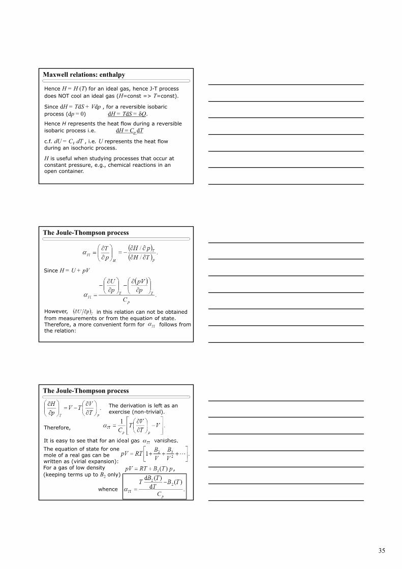
Maxwell relations: enthalpy
Hence H = H (T) for an ideal gas, hence J-T process does NOT cool an ideal gas (H=const => T=const).
Since dH = TdS + Vdp , for a reversible isobaric process (dp = 0) dH = TdS = δQ.
Hence H represents the heat flow during a reversible isobaric process i.e. dH = Cp dT
c.f. dU = CV dT , i.e. U represents the heat flow during an isochoric process.
H is useful when studying processes that occur at constant pressure, e.g., chemical reactions in an open container.
The Joule-Thompson process
Since H = U + pV
However, in this relation can not be obtained from measurements or from the equation of state. Therefore, a more convenient form for follows from the relation:
The Joule-Thompson process
The derivation is left as an exercise (non-trivial).
Therefore,
It is easy to see that for an ideal gas vanishes. The equation of state for one mole of a real gas can be written as (virial expansion):For a gas of low density (keeping terms up to B2 only)
whence
36
The Joule-Thompson process
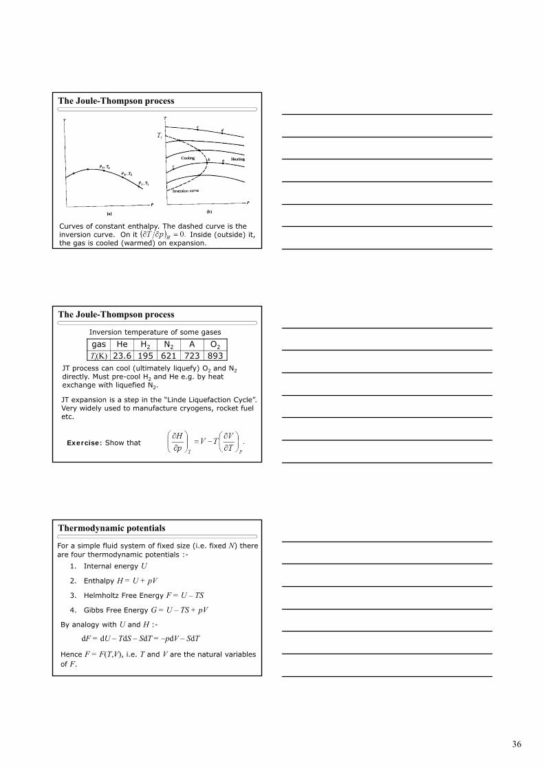
Curves of constant enthalpy. The dashed curve is the inversion curve. On it Inside (outside) it, the gas is cooled (warmed) on expansion.
The Joule-Thompson process
Exercise: Show that
gas He H2 N2 A O2
Ti(K) 23.6 195 621 723 893
Inversion temperature of some gases
JT process can cool (ultimately liquefy) O2 and N2directly. Must pre-cool H2 and He e.g. by heat exchange with liquefied N2.
JT expansion is a step in the “Linde Liquefaction Cycle”. Very widely used to manufacture cryogens, rocket fuel etc.
Thermodynamic potentials
For a simple fluid system of fixed size (i.e. fixed N) there are four thermodynamic potentials :-
1. Internal energy U
2. Enthalpy H = U + pV
3. Helmholtz Free Energy F = U – TS
4. Gibbs Free Energy G = U – TS + pV
By analogy with U and H :-
dF = dU – TdS – SdT = –pdV – SdT
Hence F = F(T,V), i.e. T and V are the natural variables of F.

37
Thermodynamic potentials: Helmholtz Free Energy
Also
hence
3rd Maxwell Relation
Since dF = –pdV – SdT the change in F represents the work done on/by a system during an isothermal (dT = 0) process.
Thermodynamic potentials: Helmholtz Free Energy
Also, dF = dU – TdS – SdT in general, butTdS = dU + pdV only for changes between equilibrium states. For changes between non-equilibrium states TdS > dU + pdV [recall example sharing 14 between 2 ensembles: dU = zero (total energy constant), dV = zero (fixed energy levels) but dS > 0 except when equilibrium reached].Hence dF =zero when equilibrium reached, dF < zeroas equilibrium is approached. Hence
For a system evolving at constant volume and temperature, equilibrium corresponds to a minimum of the system’s Helmholtz free energy.
Thermodynamic potentials: Gibbs Free Energy
dG = dU – TdS – SdT+ pdV+Vdp = – SdT + Vdp
Hence G = G(T, p) i.e. T and p are the natural variables of G.
Also
hence
4th Maxwell RelationFor a system evolving at constant pressure and temperature, equilibrium corresponds to a minimum of the system’s Gibbs free energy.

38
Thermodynamic potentials: Gibbs Free Energy
For a reversible process occurring at constant pressure and temperature (e.g. a phase change between gas and liquid such as from A to B in the figure below), the Gibbs free energy is a conserved quantity.
Thermodynamic potentials
THERMODYNAMIC POTENTIALS AND MAXWELL RELATIONS SUMMARY TABLE
The Joule process
For U = U(T,V), chain rule for partial derivatives (see PHY1026):
by dV treating T as a constant):
The free expansion of a gas into a vacuum, the whole system being thermally insulated: the total energy conserved.
hence (divide

39
The Joule and Joule-Thompson processes
3rd Maxwell relation: hence
Similarly
The Joule and Joule-Thompson processes
Hence calculate J and JT from the equation of statep = p(V,T), e.g. n moles of ideal gas: pV = nRT , hence
and hence J = JT = zero.
Real gas virial equation of state (see PHY1024):
Usually only first 2 terms are needed for good accuracy, hence
The Joule process
For all real gases (see Mandl sec 5.5), hence
J < 0, i.e. Joule expansion always cools.

40
The Joule-Thompson process
In the limit of low pressure (i.e. p0)
Hence JT > 0 (i.e. JT expansion cools) if
but JT < 0 (i.e. JT expansion heats) if
The Joule-Thompson process
The Joule-Thompson process
Tinv (inversion temperature) is maximum temperature a gas can have and still be cooled by J-T expansion.

41
The partition function
Boltzmann distribution
where
Z is the “partition function”.
a) It ensures that the pi’s are normalized, i.e.
The partition function
b) It describes how energy is “partitioned” over the ensemble i.e. states making a large contribution to Zhave a high pi hence a large share of the energy.
c) Links microscopic description of an ensemble to its macroscopic variables/ functions of state.
E.g., for an ensemble of N identical systems:
The partition function
In equilibrium at temp T
(in equilibrium)
42
The partition function
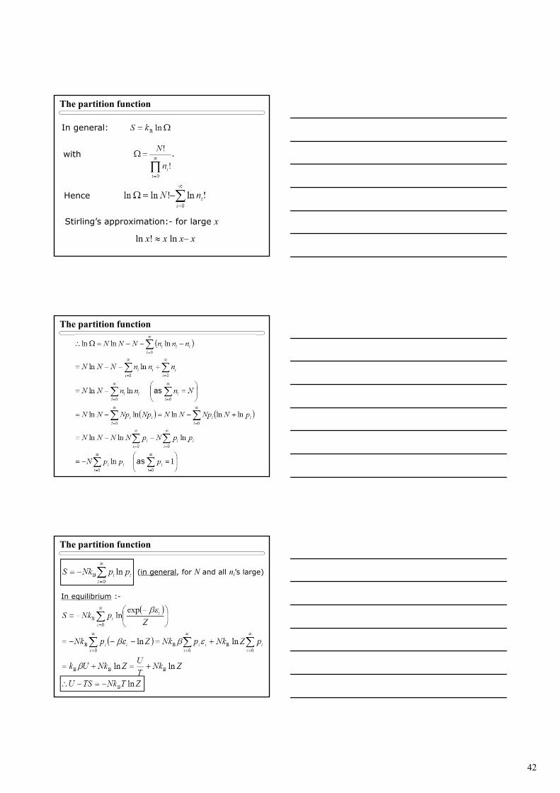
In general:
with
Hence
Stirling’s approximation:- for large x
ln x! x ln x– x
The partition function
The partition function
(in general, for N and all ni’s large)
In equilibrium :-

43
The partition function
U – TS is the Helmholtz Free Energy F, hence
(valid in equilibrium)
Einstein solid
Einstein solid – crystal of N atoms, each free to perform SHM about its equilibrium position in x, y and z directions.
Classical equipartition theorem (PHY1024) – in thermal equilibrium at temperature T, ensemble will possess a mean internal energy U given by
With being the number of degrees of freedom, i.e. the number of squared terms appearing in the expression for the total internal energy when expressed in generalized co-ordinates of position and velocity: and .
Einstein solid
E.g., for a point particle of mass m moving in 3-D
Hence = 3.
For a classical harmonic oscillator of mass m, spring constant k in 3-D,
i.e. = 6

44
Einstein solid
Hence classically, for the solid and
(Dulong-Petit law 1822),
predicts that Cv is independent of T. However, experimentally it is found that Cv 0 as T 0.
Einstein (1907): quantize the allowed energies of each of the N harmonic oscillators, such that
with being the natural frequency of the oscillator.
Einstein solid
Hence, for each oscillator
Define the Einstein temperature
Summation on RHS is a convergent geometric series, first term a = 1, common ratio
Einstein solid
The sum tends to as the number of terms tends to (see, e.g., Stroud Engineering Mathematics Programme 13), hence
Hence (exercise)
Why factor of ‘3’?

45
Einstein solid
Hence (exercise)
As T , hence i.e. tends to the classical result for high T.
As T 0,
hence because
exp(x) diverges more rapidly than xn for any finite n.
Quantum gases: momentum space
Single particle mass m confined to a cubic container (3-D potential well) side length L.
Describe particle via a wavefunction (x,y,z) satisfying the energy eigenvalue equation :-
Solutions E and (x,y,z) are the energy eigenvalues and stationary states of the particle.
Boundary conditions: (0,y,z) = (L,y,z) = (x,0,z) = (x,L,z) = (x,y,0) = (x,y,L) = 0
Quantum gases: momentum space
Solution :-
(ditto y,z ); nx = 1, 2, 3 … (ditto ny, nz )

46
Quantum gases: momentum space
Momentum space picture :-
Quantum gases: momentum space
Allowed states form a cubic lattice, lattice constant .
Hydrogen atom at room temp confined to 1m3:
Compare with
Hence momentum states are very finely spaced can often treat as forming a continuum.
Quantum gases
Gas of N particles in a cubic container, side length L.
If N/nstates << 1 we have a ‘classical’ gas.
If N/nstates ~ 1 we have a ‘quantum’ (or ‘quantal’) gas.
Behaviour of a quantum gas is strongly determined by the Pauli Exclusion Principle:
Any number of bosons can occupy a given quantum state but only one fermion can occupy a given quantum state.
Half-integer spin particles (e.g. e, p, n) are ‘Fermions’. Integer-spin particles (e.g. , phonon) are ‘Bosons’.

47
Quantum gases
Consider , the mean energy of each of the N particles in the container:
nstates volume of momentum space enclosed by an octant of
radius pmean / volume occupied by one state
Hence
Quantum gases
Hence a gas becomes quantum when the mean inter-particle spacing becomes comparable with the particles’ de Broglie wavelength.
Consider Hydrogen at STP, molar volume 22.410–3 m3. Mean spacing = (22.410–3/61023)1/3 = 310–9 m. At room temp,
Only 1 in 1000 states typically occupied hence it is safe to treat as a “classical” gas i.e. rules for filling states are unimportant.
Quantum gases
Now consider gas of conduction electrons in a metal, density typically 1028 m–3.
Hence, conduction electrons form a quantum gas, i.e., the rules for filling states are important. Electrons are fermions so only one particle can occupy a given quantum state.
As T0 the electrons will crowd into the lowest available energy level. Unlike a classical ensemble they cannot all move into the ground state, because only one particle is allowed per state. Instead they will fill all available states up to some maximum energy, the Fermi energy EF
Mean spacing = (1028)–1/3 = 0.510–9 m.

48
Fermi gas
As T 0, fermions will fill all available states up to some maximum energy EF or equivalently a maximum momentum pF, the Fermi momentum.
Hence number of states contained within an octant of momentum space, radius pF = N/2 (because each translational momentum state actually comprises TWO distinct quantum states, with the electron spin ‘up’ and spin ‘down’ respectively).
Fermi gas
Writing N/V = n, the particle number density,
E.g., for the conduction electrons in a metal
Fermi-Dirac distribution
Equilibrium distribution of energy U over N particles when
a) only ONE particle per state is allowed (c.f. Boltzmann distribution, any number of particles per state were allowed).
b) the particles are indistinguishable (c.f. Boltzmann distribution, the particles were distinguishable).
Quantum states form a densely-spaced near-continuum. Divide these states into “bands” of nearly identical energy. Hence band ihas a characteristic energy Ei, number of states ωi and holds niparticles.
Total number of microstates Ωtotal is given by
where Ωi = the total number of ways to choose ni indistinguishable objects from ωi possibilities (c.f. coin-flipping).

49
Fermi-Dirac distribution
Hence
As with the Boltzmann distribution, we obtain the equilibrium distribution by seeking the ni’s that maximise ln Ωtotal subject to the constraints
Solution (see supplement sheet 4):
- Fermi-Dirac distribution
Here EF is a constant (the Fermi Energy).
Bose-Einstein distribution
Bosons, unlike fermions, are not subject to the Pauli exclusion principle: an unlimited number of particles may occupy the same state at the same time. This explains why, at low temperatures, bosons can behave very differently from fermions; all the particles will tend to congregate at the same lowest-energy state, forming what is known as a Bose–Einstein condensate.Bose-Einstein statistics was introduced for photons in 1924 by Bose and generalized to atoms by Einstein in 1924-25.
- Bose-Einstein distribution
Bose-Einstein distribution
For bosons
As with the Boltzmann and Fermi distributions, we obtain the equilibrium distribution by seeking the ni’s that maximise
ln Ωtotal subject to the constraints

50
Classical limit
Fermi-Dirac and Bose-Einstein distributions:
+Fermi-Dirac distribution
- Bose-Einstein distribution
This corresponds to the Boltzmann distribution.
Thus,


![[Roger bowley, mariana_sánchez]_introductory_stat(bookos.org)](https://static.fdocuments.us/doc/165x107/555f2974d8b42a93658b5028/roger-bowley-marianasanchezintroductorystatbookosorg.jpg)


![[Gordon Bowley] How to Deal With Death and Probate(BookFi.org)](https://static.fdocuments.us/doc/165x107/55cf9038550346703ba4095a/gordon-bowley-how-to-deal-with-death-and-probatebookfiorg.jpg)