From Aggregate Betting Data

to Individual Risk Preferences∗

Pierre-Andre Chiappori† Bernard Salanie‡ Francois Salanie§

Amit Gandhi¶

October 17, 2012

Abstract

As a textbook model of contingent markets, horse races are an attractive environ-

ment to study the attitudes towards risk of bettors. We innovate on the literature by

explicitly considering heterogeneous bettors and allowing for very general risk prefer-

ences, including non-expected utility. We build on a standard single-crossing condition

on preferences to derive testable implications; and we show how parimutuel data allow

us to uniquely identify the distribution of preferences among the population of bettors.

We then estimate the model on data from US races. Within the expected utility class,

the most usual specifications (CARA and CRRA) fit the data very badly. Our results

show evidence for both heterogeneity and nonlinear probability weighting.

∗This paper was first circulated and presented under the title ”What you are is what you bet: elicitingrisk attitudes from horse races.” We thank many seminar audiences for their comments. We are especiallygrateful to Jeffrey Racine for advice on nonparametric and semiparametric approaches, and to Simon Woodfor help with his R package mgcv. Bernard Salanie thanks the Georges Meyer endowment for its supportduring a leave at the Toulouse School of Economics. Pierre Andre Chiappori gratefully acknowledges financialsupport from NSF (Award 1124277.)†Columbia University. Email: pc2167@columbia.edu‡Columbia University. Email: bsalanie@columbia.edu§Toulouse School of Economics (Lerna, Inra, Idei). Email: salanie@toulouse.inra.fr¶University of Wisconsin-Madison. Email: agandhi@ssc.wisc.edu

1

1 Introduction

There is mounting experimental evidence that risk attitudes are massively heterogeneous.

To quote but a few examples, Barsky et al. (1997) use survey questions and observations of

actual behavior to measure relative risk aversion. Results indicate that this parameter varies

between 2 (for the first decile) and 25 (for the last decile), and that this heterogeneity is

poorly explained by demographic variables. Guiso and Paiella (2006) report similar findings,

and use the term ‘massive unexplained heterogeneity’. Chiappori and Paiella (2011) observe

the financial choices of a sample of households across time, and use these panel data to show

that while a model with constant relative risk aversion well explains each household’s choices,

the corresponding coefficient is highly variable across households (its mean is equal to 4.2, for

a median equal to 1.7). (Distributions of) risk aversions have also been estimated using data

on television games (Beetsma and Schotman, 2001), demand for insurance (Cohen and Einav,

2007) or risk sharing within closed communities (Bonhomme et al. 2012, Chiappori et al.

2012). These papers and many others indicate that attitudes towards risk and uncertainty are

widely heterogeneous, and that recognizing this heterogeneity may be crucial to understand

observed behavioral patterns.

The various attempts just mentioned share a common feature: they all rely on data on

individual behavior. Indeed, a widely shared view posits that microdata are indispensable to

analyze heterogeneous attitudes to risk. The present paper challenges this claim. It argues

that, in many contexts, the distribution of risk aversion can be nonparametrically identified,

even in the absence of data on individual decisions; we only need to use the (aggregate)

conditions that characterize an equilibrium, provided that these equilibria can be observed

on a large set of different “markets”. While a related approach has often been used in other

fields (e.g., empirical industrial organization), to the best of our knowledge, it has never been

applied to the estimation of a distribution of individual attitudes towards risk.

Specifically, we focus on the case of horse races, which can be seen as a textbook example

for financial markets, and for which large samples are available. The races we consider

use parimutuel betting; that is, those lucky bettors that have bet on the winning horse

share the total amount wagered in the race (minus the organizer’s take)—so that observing

the odds of a horse is equivalent to observing its market share. The intuition underlying

our approach can be summarized as follows. Assume that, for any given race, we can

simultaneously observe both the odds and the winning probability of each horse. Clearly,

the relationship between these two sets of variables depends on (the distribution of) bettors’

2

attitudes toward risk. To take but a simple example, with risk neutral bettors odds would

be directly proportional to winning probabilities. As we shall see, a linear relationship of

this kind is largely counterfactual. But a basic insight remains: the variation in odds (or

market shares) from race to race as a function of winning probabilities conveys information

on how bettors react to given lotteries. If we observe a large enough number of “markets”

(here races) with enough variations (here in odds and winning probabilities), and under the

assumption that the population of bettors has the same distribution of preferences in these

markets, we may learn about the characteristics of this distribution from the sole observation

of probabilities and resulting odds on these different markets.

This leads to two fundamental questions. One is testability: can one derive, from some

general, theoretical representation of individual decision under uncertainty, testable restric-

tions on equilibrium patterns—as summarized by the relationship between probabilities and

odds? The second issue relates to identifiability: under which conditions is it possible to

recover, from the same equilibrium patterns, the structure of the underlying model—i.e., the

distribution of individual preferences?

While additional restrictions are obviously necessary to reach this dual goal, we show

that they are surprisingly mild. Essentially, three assumptions are needed. One is that,

when choosing between lotteries, agents only consider their direct outcomes: the utility

derived from choosing one of them (here, betting on a given horse) does not depend on the

characteristics of the others. While this assumption does rule out a few existing frameworks

(e.g., those based on regret theory), it remains compatible with the vast majority of models

of decision making under uncertainty. Secondly, we assume that agents’ decisions regarding

bets are based on the true distribution of winning probabilities. An assumption of this kind

is clearly indispensable in our context; after all, any observed pattern can be rationalized

by a well chosen distribution of ad-hoc, individual beliefs. Note, however, that we do not

assume these probabilities are used in a linear way; on the contrary, we allow for the type

of probability (or belief) distorsions emphasized by modern decision theory, starting with

Yaari’s dual model or Kahneman and Tversky’s cumulative prospect theory. In other words,

we accept that a given probability can have different “weights” in the decision process of

different agents; but, for parsimony, we choose to model this heterogeneity as individual-

specific deformations of a common probability distribution.1 Our last assumption is related

to the form of preference heterogeneity among agents. Specifically, we assume that it is one-

1Of course, such a formulation implies some restrictions on observed behavior. For instance, most proba-bility deformation functions are monotonic; using one of these therefore implies that individual deformationscannot reverse the probability ranking of two events.

3

dimensional, and satisfies a standard single-crossing condition. Note that the corresponding

heterogeneity may affect preferences, beliefs (or probability deformation) or both; in that

sense, our framework is compatible with a wide range of theoretical frameworks.

Our main theoretical result states that, under these three conditions, an equilibrium

always exists, is unique, and that the answer to both previous questions is positive: one can

derive strong testable restrictions on equilibrium patterns, and, when these conditions are

fulfilled, one can identify the distribution of preferences in the population of bettors.

We then provide an empirical application of these results. In practice, we introduce the

crucial concept of normalized fear of ruin (NF), which directly generalizes the fear or ruin

index introduced in an expected utility setting by Aumann and Kurz (1977). We argue that

this concept provides the most adequate representation of the risk/return trade off for the

type of binomial lotteries under consideration in our context. Intuitively, the NF measures

the elasticity of required return with respect to probability, along an indifference curve be-

tween lotteries ; as such, it can be defined under expected utility maximization (in which

case it does not depend on probabilities), but also in more general frameworks, entailing for

instance probability deformations or various non-separabilities. We show that the identifi-

cation problem boils down to recovering the NF index as a function of odds, probabilities

and a one-dimensional heterogeneity parameter. We provide a set of necessary and suffi-

cient conditions for a given function to be an NF; these provide the testable restrictions

mentioned above. Also, we show that, under these conditions, the distribution of NF is non

parametrically identified.

Finally, we estimate our model on a sample of more than 25,000 races involving some

200,000 horses. We derive a new empirical strategy to non parametrically identify the rela-

tionship between the NF index and its determinants (i.e., odds, probabilities and an hetero-

geneity parameter). Since the populations in the various “markets” must, in our approach,

have similar distributions of preferences, we focus on races taking place during weekdays,

on urban race fields. We show that our restrictions regarding both the one-dimensional

heterogeneity and the single crossing conditions fit the data well, at least in the regions

in which heterogeneity can be identified with enough power. Last but not least, we derive

a non parametric estimation of both a general model (involving unrestricted non expected

utility with general one-dimensional heterogeneity) and several submodels (including homo-

geneous and heterogenous versions of expected utility maximization, Yaari’s dual model and

rank-dependent expected utility).

Our empirical conclusions are quite interesting. First, we confirm that the role of het-

4

erogeneity is paramount; even the most general models perform poorly under homogeneity.

Second, both the shape of individual utilities and its variations across agents are complex. For

instance, under our preferred specification, a significant fraction of bettors are risk averse for

some bets and risk loving for others. This suggests that the parametric approaches adopted

in much applied work should be handled with care, at least when applied to the type of data

considered here, as they may imply unduly restrictive assumptions.2

An obvious limitation of our study is that it considers a selected (although quite large)

population, namely individuals betting in horse races. Clearly, this subpopulation may not

be representative of the general public. Still, we believe that gathering information about the

distribution of preferences in this population may provide interesting insights on individual

attitudes to risk in general. Moreover, even though the details of our approach are case

specific, the general idea—recovering attitudes to risk from equilibrium patterns observed

on many markets—can and should be transposed to different contexts.

1.1 Related Literature

The notion that the form of a general equilibrium manifold may generate testable re-

strictions is not new, and can be traced back to Brown and Matzkin (1996) and Chiappori

et al. (2002, 2004)—the latter in addition introduce the idea of recovering individual pref-

erences from the structure of the manifold. But these papers have not, to the best of our

knowledge, lead to empirical applications. Our contributions here are most closely related to

the literature on estimating and evaluating theories of individual risk preferences, and also

to the literature on identification of random utility models. There is now a large literature

that tests and measures theories of individual risk preference using laboratory methods (see

e.g., Bruhin et al (2010) and Andreoni and Sprenger (2010) for two recent contributions.)

There is also a sizable literature that directly elicits individual risk preferences through sur-

vey questions (see e.g., Barsky et al (1997); Bonin et al (2007); Dohmen et al (2011)) and

correlates these measures with other economic behaviors. The literature on studying risk

preferences as revealed by market transactions is much more limited. The primary avenues

that have been pursued are insurance choices (see e.g., Cohen and Einav (2007); Sydnor

(2010); and Barseghyan et al (2011)) and gambling behavior (see e.g., Andrikogiannopoulou

(2010)). However all of these studies fundamentally exploit individual level demand data to

2For instance, under such commonly used representations as CARA or CRRA preferences, any givenindividual is either always risk averse or always risk loving.

5

estimate risk preferences and document heterogeneity.

The literature on estimating risk preferences from market level data has almost exclusively

used a representative agent paradigm. Starting with Weitzman (1965), betting markets have

served as a natural source of data for representative agent studies of risk preferences due

to the textbook nature of the gambles that are offered. In the context of racetrack betting,

Jullien and Salanie (2000) and Snowberg and Wolfers (2010) provide evidence showing that

a representative agent with non-linear probability weighting better explains the pattern of

prices at the racetrack as compared to an expected utility maximizing representative agent.

Aruoba and Kearney (2011) present similar findings using cross sectional prices and quan-

tities from state lotteries. These representative agent studies of betting markets stand in

contrast to a strand of research that has emphasized belief heterogeneity as an important

determinant of equilibrium in security markets. Ottaviani and Sorensen (2010) and Gandhi

and Serrano-Padial (2011) argue that heterogeneity of beliefs and/or information of risk

neutral agents can explain the well known favorite longshot bias that empirically character-

izes betting market odds, and Gandhi and Serrano-Padial furthermore estimate the degree

of belief heterogeneity revealed by the odds. In contrast, our aim here is to fully explore

the consequences of heterogeneity in preferences. Our paper is the only one to date that

nonparametrically identifies and estimates heterogeneous risk preferences from market level

data. Furthermore, while our theoretical framework excludes heterogeneity in beliefs, it

allows for heterogeneity in probability weighting across agents; and our nonparametric ap-

proach allows us to compare this and other theories (such as heterogeneity in risk preferences

in an expected utility framework.)

Finally, our paper makes a contribution to the identification of random utility models of

demand. Random utility models have become a popular way to model market demand for

differentiated products following Bresnahan (1987), Berry (1994), and Berry et al. (1995).

A lingering question in this literature is whether preference heterogeneity can indeed be

identified from market level observations alone. Along with Chiappori, Gandhi, Salanie

and Salanie (2009), our paper shows that a non-parametric model of vertically differen-

tiated demand can be identified from standard variation in the set of products available

across markets. In particular we exploit a one dimensional source of preference heterogene-

ity that satisfies a standard single crossing condition consistent with vertically differentiated

demand. We show that the identification of inverse demand from the data allows us to

non-parametrically recover this class of preferences. This stands in contrast to recent work

by Berry and Haile (2010), who use full-support variation in a “special regressor” to show

6

that an arbitrary random utility model can be recovered from inverse demand3. We instead

show identification of random utility without a special regressor by exploiting the additional

restriction that random utility satisfies the single crossing structure.

We present the institution, assumptions, and the structure of market equilibrium in sec-

tion 2. In section 3, we explain the testable restrictions on observed demand behavior implied

by the model, and we show that these restrictions are sufficient to identify preferences. Sec-

tion 4 describes the data, while Section 5 discusses the estimation strategy. We describe our

results in Section 6, and Section 7 concludes.

2 Theoretical framework

Parimutuel We start with the institutional organization of parimutuel betting. Consider

a race with i = 1 . . . n horses. The simplest bets are “win bets”, i.e. bets on the winning

horse: each dollar bet on horse i pays a net return Ri if horse i wins, and is lost otherwise.

Ri is called the odds of horse i, and in parimutuel races it is determined by the following

rule: all money wagered by bettors constitutes a pool that is redistributed to those who

bet on the winning horse, apart from a share t corresponding to taxes and a house “take”.

Accordingly, if si is the share of the pool corresponding to the sums wagered on horse i, then

the payment to a winning bet of $1 is

Ri + 1 =1− tsi

(1)

Hence odds are not set by bookmakers; instead they are determined by the distribution (s1,

. . . , sn) of bets among horses. Odds are mechanically low for those horses on which many

bettors laid money (favorites), and they are high for outsiders (often called longshots)4.

Because shares sum to one, these equations together imply

1

1− t=∑i

1

Ri + 1(2)

Hence knowing the odds (R1, . . . , Rn) allows to compute both the take t and the shares in

the pool (s1, . . . , sn).

3See also Gautier-Kitamura (2012) on the binary choice model.4According to this formula odds can even be negative, if si is above (1− t)—it never happens in our data.

7

Probabilities We now define a n-horse race (p, t) by a vector of positive probabilities

p = (p1, . . . , pn) in the n-dimensional simplex, and a take t ∈ (0, 1). Note that pi is the

objective probability that horse i wins the race. Our setting is thus compatible with tradi-

tional models of decision under uncertainty, in which all agents agree on the probabilities,

and these probabilities are unbiased. Such a setting singles out preferences as the driving

determinant of odds; it accords well with empirical work that shows how odds discount

most relevant information about winning probabilities5. It is also consistent with the famil-

iar rational expectations hypothesis (in fact we will later show that a rational expectations

equilibrium exists and is unique in our setting). It is important to stress, however, that our

framework is also compatible with more general models of decision uncertainty. In partic-

ular, it allows (among other things) for the type of probability weighting that characterizes

many non-expected utility functionals (whereby the actual decision process may involve ar-

bitrary functions of the probabilities). Moreover, these probability deformations may, as we

shall see, be agent-specific. In other words, our general framework encompasses both “tradi-

tional” models, in which agents always refer to objective probability and heterogeneity only

affects preferences, and more general versions in which the treatment of the probabilities is

heterogenous among agents. As we shall see, the only strong restriction we put is on the

dimension of the heterogeneity under consideration, not on its nature.

Following the literature to date6, we endow each bettor with a standardized unit bet size

that he allocates to his most preferred horse in the race. In particular, we do not model

participation, and bettors are not allowed to opt out. Therefore the shares (si) in the pool

defined above can be identified to market shares. Any bettor looks on a bet on horse i as

a lottery that pays returns Ri with probability pi, and pays returns (−1) with probability

(1− pi). We denote this lottery by (Ri, pi), and call it a gamble. By convention, throughout

the paper we index horses by decreasing probabilities (p1 > · · · > pn > 0), so that horse 1 is

the favorite.

Risk neutrality as a benchmark As a benchmark, consider the case when bettors are

risk-neutral, and thus only consider the expected gain associated to any specific bet7. Equi-

5See Sung and Johnson (2008) and Ziemba (2008) for recent surveys on the informational efficiency ofbetting markets.

6See Weitzman (1965), Jullien and Salanie (2000), Snowberg and Wolfers (2010), among others.7Clearly, a risk neutral player will not take a bet with a negative expected value unless she derives some

fixed utility from gambling. The crucial assumption, here, is that this “gambling thrill”, which explains whysuch people gamble to start with, does not depend on the particular horse on which the bet is placed—sothat, conditional on betting, bettors still select the horse that generates the highest expected gain.

8

librium then requires expected values to be equalized across horses. Since bets (net of the

take) are redistributed, this yields:

piRi − (1− pi) = −t

which, together with (2), gives probabilities equal to

pni (R1, . . . , Rn) =

1

Ri + 1∑j

1

Rj + 1

=1− t

1 +Ri

= si. (3)

By extension, for any set of odds (R1, ..., Rn), the above probabilities pni will be called

the risk-neutral probabilities. These probabilities are exactly equal to the shares si in the

betting pool, as defined in (1) and (2). Many stylized facts (for instance, the celebrated

favourite-longshot bias) can easily be represented by comparing the “true” probabilities with

the risk-neutral ones—more on this below.

2.1 Preferences and single-crossing

Preferences over gambles We consider a continuum of bettors, indexed by a parameter

θ. In our setting, a gamble (a horse) is defined by two numbers: the odds R and the winning

probability p. To model individual choices, we assume that each bettor θ is characterized

by a utility function V (R, p, θ), defined over the set of gambles and the set of individuals.

Thus, in a given race, θ bets on the horse i that gives the highest value to V (Ri, pi, θ). Since

we treat V nonparametrically, we can without loss of generality normalize the distribution

of θ so that it is uniform on [0, 1]. In the end, we therefore define V on IR+ × [0, 1]× [0, 1].

Note that V is a utility function defined on the space of gambles. As such, it is compatible

with expected utility, but also with most non expected utility frameworks; a goal of this

paper is precisely to compare the respective performances of these various models for the

data under consideration. As usual, V is defined only ordinally, i.e. up to an increasing

transform. Finally, the main restriction implicit in our assumption is that the utility derived

from betting on a given horse does not depend on the other horses in the race; we thus rule

out models based for instance on regret theory8, and generally any framework in which the

valuation of any bet depends not only on the characteristics of the bet but also on the whole

8See e.g. Gollier and Salanie (2006).

9

set of bets available9.

We will impose several assumptions on V . We start with very weak ones:

Assumption 1 V is continuously differentiable almost everywhere; and it is increasing with

R and p.

Differentiability is not crucial; it just simplifies some of the equations. Our framework

allows for a kink at some reference point for instance, as implied by prospect theory. The

second part of the assumption reflects first-order stochastic dominance: bettors prefer bets

that are more likely to win, or that have higher returns when they do.

The Normalized Fear of Ruin (NF) When analyzing individual behavior under risk,

a fundamental notion is the trade-off between risk and return; one goal of the present paper

is precisely to identify this trade-off from observed choices. Technically, the trade-off can be

described in several ways. One is the marginal rate of substitution10 w:

w(R, p, θ) ≡ VpVR

(R, p, θ) > 0

Since the utility function V is only defined up to an increasing transform, the properties of

w fully determine the bettors’ choices among gambles. In practice, however, we shall focus

on a slightly different index, that we call the normalized fear-of-ruin (NF ):

NF (R, p, θ) ≡ p

R + 1

VpVR

(R, p, θ) =p

R + 1w(R, p, θ) > 0

Using NF rather than more traditional measures of risk-aversion has several advantages.

It is unit-free, as it is the elasticity of required return with respect to probability on an

indifference curve:

NF = − ∂ log(R + 1)

∂ log p

∣∣∣∣V

.

As such it measures the local trade off between risk and return. Moreover, it has a “global”

interpretation for the type of binomial lotteries we are dealing with. Indeed, for a risk-neutral

agent the NF index is identically equal to one. An index above one indicates that the agent

is willing to accept a lower expected return p(R + 1)− 1 in exchange for an increase in the

probability p. Conversely, if an agent with an index below one is indifferent between betting

9We could accommodate characteristics such as the origin of the horse, as long as they are in the data.10Throughout the paper subscripts to functions indicate partial derivatives.

10

on a favorite (p, R) and a longshot (p′ < p, R′ > R), then it must be that the expected

return on the longshot is below that on the favorite. For instance, in a representative agent

context, the favorite-longshot bias is explained by the representative agent having a NF index

below one. Remember, however, that our approach entails heterogeneous bettors; as such, it

is more general, and can accommodate the existence of bettors with different NF indices.

The expected utility case In an expected utility framework, the NF index has a simple

expression. Indeed, normalizing to zero the utility u(−1, θ) of losing the bet, we have that:

V (R, p, θ) = pu (R, θ)

and therefore

NF (R, p, θ) =1

R + 1

u

uR(R, θ)

so that the NF index is independent from the probability p. The ratio u/uR was called the

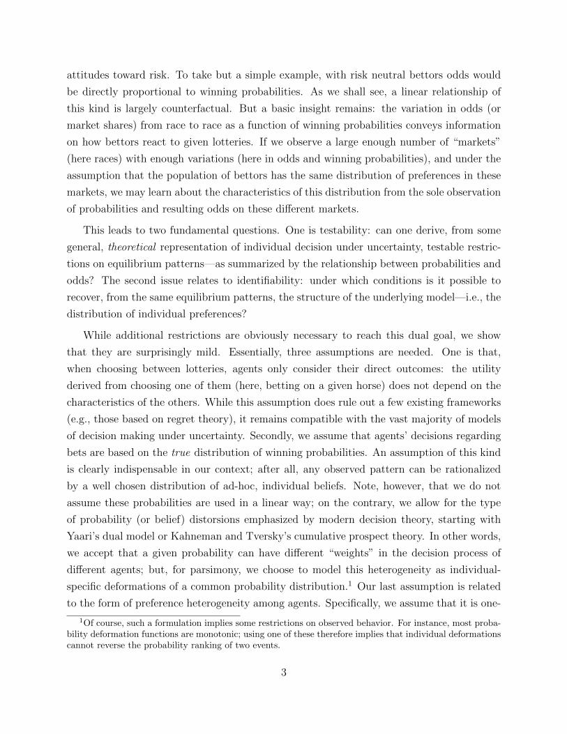
fear of ruin (FoR) index by Aumann and Kurz (1977). Geometrically, NF (R, p, θ) is the

ratio of two slopes on the graph of the utility function: that of the chord linking two points,

(−1, 0) (which represents losing the bet) and (R, u (R)) (winning), and that of the tangent

to the utility graph at (R, u (R)) (see Figure 1.)

The properties of the NF index in the expected utility case are well known (see Foncel

and Treich, 2005). A sufficient condition for an agent to have a higher NF index than

another agent at all values of R is that the former be more risk-averse than the latter11.

Consequently, if the agent is risk averse, then his NF index is larger than 1; if he is risk-

loving, it is smaller than 1. Lastly, while the NF index need not be monotonic in R, specific

functional forms may generate additional properties. For example, an agent with constant

absolute risk-aversion is either risk-averse (so that her NF is above 1 and increasing) or

risk-loving (and then her NF is below 1 and decreasing). The same “fanning out” holds in

the generalized CRRA case, for which

u(R) =(W +R)1−γ − (W − 1)1−γ

1− γ

where W > 1 is the agent’s wealth.

11Recall that u is more risk-averse than v if there exists an increasing and concave function k such thatu = k(v). Given our normalization u(0) = v(0) = 0, this implies that k is such that k(x)/x decreases withx. This property is equivalent to the fact that u has a higher NF index than v, at any value of R (see Fonceland Treich, 2005).

11

-1 0 R

u(R)/(1+R)

u’(R)

u(R)

Figure 1: Normalized Fear-of-ruin NF under Expected Utility

These results suggest that simple parametric forms should in this context be handled with

great care, as they may turn out to be unduly restrictive. It is often argued that CARA or

CRRA can be considered as acceptable approximations of more general utilities. This claim,

however, appears quite debatable when one considers the NF index, which is the crucial

determinant of choices in our context. As we shall see, our nonparametric estimates show

NF indices that tend to fan in rather than fan out, and can cross the NF = 1 line.

Single crossing assumption We now introduce two additional requirements. The first

one will be used when proving the existence of a rational expectations equilibrium:

Assumption 2 For any θ, R, p > 0:

• for any p′ > 0, there exists R′ such that V (R, p, θ) < V (R′, p′, θ);

• for any R′, there exists p′ > 0 such that V (R, p, θ) > V (R′, p′, θ).

Assumption 2 is very weak: it requires that any higher return can be compensated by a

lower probability of winning, and vice versa. The next assumption is crucial: it imposes a

single crossing property that drives our approach to identification.

12

Assumption 3 (single-crossing) Consider two gambles (R, p) and (R′, p′), with p′ < p.

If for some θ we have

V (R, p, θ) ≤ V (R′, p′, θ)

then for all θ′ > θ

V (R, p, θ) < V (R′, p′, θ′).

Given first-order stochastic dominance as per Assumption 1, if θ prefers the gamble with

the lowest winning probability (p′ < p) then it must be that its odds are higher (R′ > R),

so that the gamble (R′, p′) is riskier. Assumption 3 states that since θ prefers the riskier

gamble, any agent θ′ above θ will too. The single-crossing assumption thus imposes that

agents can be sorted according to their “taste for risk”: higher θ’s prefer longshots, while

lower θ’s prefer favorites.

If we slightly strengthen Assumption 1 to require that V be differentiable everywhere on

some open set O, then Assumption 3 has a well-known differential characterization, which

we state without proof:

Lemma 1 Assumption 3 holds on O if and only if, for any (R, p, θ) in O, the marginal rate

of substitution w(R, p, θ), or equivalently the normalized fear-of-ruin index NF (R, p, θ), is

decreasing in θ.

The precise scope of this condition can be better seen on a few examples.

1. Expected utility: as above, we normalize to zero the utility of losing the bet, so that

V (R, p, θ) = pu(R, θ).

Single-crossing holds if and only if the normalized fear-of-ruin is decreasing in θ. A sufficient

condition is that lower θ’s be more risk-averse at any value of R. For instance, in the CARA

case, consider a population of bettors indexed by their absolute risk-aversion λ:

u(R, λ) =exp(λ)− exp(−λR)

λ

where λ follows a distribution with c.d.f. Φ. Then it is easily seen that

NF (R, p, θ) =1

R + 1

u

uR=

exp (λ (1 +R))− 1

λ(1 +R)

13

increases with λ. If we define θ as 1−Φ(λ), then by construction θ is uniformly distributed

on [0, 1], and NF decreases in θ, so that Assumption 3 holds. A similar result holds for

CRRA functions for instance.

2. Rank-Dependent Expected Utility Theory RDEU enriches the previous frame-

work by allowing for a deformation of probabilities. It requires that there exist two functions

G and u such that the utility V can be written

V (R, p, θ) = G (p, θ)u(R, θ).

For Assumption 1 to hold, the probability weighting function G must increase in p and the

utility function u must increase in R. In general, both functions may vary with θ.

For the power specification

G(p, θ) = pc(θ)

it is easily seen that one is back to the expected utility case by raising V at the power (1/c(θ)).

This implies that in the RDEU case, one can only identify variations in the elasticity of G

with respect to probability p. To see this differently, the NF index is a product of two terms:

NF (R, p, θ) =p

R + 1

VpVR

=pGp

G

1

R + 1

u

uR. (4)

The second term is the NF index for an expected utility maximizer with utility u. The

first term is the NF index that would obtain if u were linear in R for all θ, as in the “dual

expected utility” model of Yaari (1987):

V (p,R, θ) = G(p, θ)(R + 1),

in which agents are heterogeneous in how they weigh probabilities. For Yaari-like preferences

the NF index is independent of R; and single-crossing requires that Gp/G, which is positive,

be decreasing in θ. In words, this means that larger θ’s overestimate small probabilities

more (or underestimate them less) than smaller θ’s. Again, this allows us to account for

some heterogeneity in beliefs.

Note that since Yaari’s model sets the elasticity of u to one, we can identify the elasticity

of G and its variations with θ in this more restricted model. More generally, our empirical

approach will allow us to elucidate the heterogeneity in both terms of (4).

14

3. Robust control Our framework is also compatible with more complex settings; in

particular, it is compatible with ambiguity. For instance, Hansen and Sargent (e.g. in their

2007 book, or Hansen 2007) model an agent with a von Neumann-Morgenstern utility index

u who recognizes that the true probability distribution over outcomes m = (m1, . . . ,mn) is

uncertain and may differ from p. In our simple setting, the utility from betting on horse i

becomes

minm

[miu(Ri) + a(θ)e(m,p)]

where e(m,p) is the relative entropy function that penalizes distortions from p:

e(m,p) =∑j

mj log(mj

pj)

The positive coefficient a(θ) measures how much bettor θ pays attention to probability

distortions. In our static case, such a departure from the standard expected utility framework

amounts to considering an expected utility maximizer with beliefs p and preferences

u(R, θ) = 1− exp(−u(R)/a(θ))

which is a special case of heterogenous expected utility as the “reference utility” u is the

same for all agents.

It is easy to see that the normalized fear-of-ruin index associated to u is

NF (R, θ) =exp(u(R)/a(θ))− 1

u(R)/a(θ)

u(R)

u′(R)(R + 1);

it increases with θ if and only if a increases with θ. Hence single-crossing obtains under this

simple condition on a.

4. Others Many other families of preferences, such as cumulative prospect theory, also

fit within our setting—although the single-crossing condition becomes more complicated.

Others may only be accommodated under some restrictions. For instance, the reference-

dependent theory of choice under risk of Koszegi and Rabin (2007) characterizes a bettor

with a utility index m and a function µ applied to deviations with respect to reference

outcomes, so that perceived utility in a state in which r was expected and w obtains would

15

be

u(w|r) = m(w) + µ (m(w)−m(r)) .

Simple calculations show that in their choice-acclimating personal equilibrium12, the bettor

would focus her bets on horses i that maximize (still normalizing m(−1) = 0)

V (Ri, pi) = pim(Ri) + pi(1− pi) (µ(m(Ri)) + µ(−m(Ri))) .

For µ ≡ 0 this is just expected utility. Now Koszegi and Rabin take the function µ to be

increasing with a concave kink in zero; then the factor µ(m(Ri)) + µ(−m(Ri)) is negative

and if it becomes large, this choice functional may violate stochastic dominance.

Limitations Our approach has two main limitations. First, we require agents to only pay

attention to consequences. As mentioned above, some models of decision under uncertainty

relax this assumption (a classical example being the notion of regret); these are not compat-

ible with our setting. Second, we only allow for one dimension of heterogeneity. On the one

hand, the single-crossing assumption excludes, strictly speaking, the case of a fully homoge-

neous population considered in Jullien and Salanie (2000): when V is independent of θ, the

strict inequality in the assumption cannot hold. Nevertheless, homogeneity is easily dealt

with as a limiting case, as we shall see. More damaging is the opposite restriction—namely,

we do not consider models involving a richer representation of heterogeneity. For instance,

while our approach is compatible with models involving heterogeneity in both preferences

and beliefs, these two dimensions must in our context be governed by the same parameter,

which obviously restricts the generality of our approach. Multidimensional nonparametric

heterogeneity is a very difficult (although not necessarily hopeless) problem, which is left for

future work.

2.2 Market Shares and Equilibrium

The winning probabilities are assumed exogenous and characterize the race. In contrast,

the odds are endogenous: the bettors’ behavior determines market shares, which in turn

determine odds through the parimutuel rule (1). In such a setting, it is natural to rely on

the concept of rational expectations equilibria: agents determine their behavior given their

anticipations on odds, and these anticipations are fulfilled in equilibrium. We now show that

12See Definition 3 on page 1058 in Koszegi and Rabin (2007).

16

for our framework, a rational expectations equilibrium exists. Moreover the characterization

of the equilibrium condition in terms of the single crossing assumption will provide the key

link to identification of preferences (proofs for this section are relegated to Appendix 1).

Let us assume that the families p and R are given, and known to all agents. Each agent

then optimizes on which horse to bet on, and a simple consequence of the single crossing

condition is the following:

Lemma 2 Suppose that p and R are such that all market shares are positive: si > 0, i =

1, . . . , n. Then there exists a family (θj)j=0,...,n, with θ0 = 0 < θ1 < · · · < θn−1 < θn = 1,

such that:

• for all i = 1, . . . , n, if θi−1 < θ < θi then bettor θ strictly prefers to bet on horse i than

on any other horse;

• for all i < n we have

V (pi, Ri, θi) = V (pi+1, Ri+1, θi) (5)

In words: under single crossing, if we rank horses by increasing odds, we have a partition

of the set of bettors into n intervals, each of them gathering bettors who bet for the same

horse. The bounds of the intervals are defined by an indifference condition; namely, for

i = 1, . . . , n − 1, there exists a marginal bettor θi who is indifferent between betting on

horses i and i+ 1.

As a simple corollary, because the distribution of θ is uniform the market shares si for

horse i = 1, . . . , n can be expressed as

si = θi − θi−1

or equivalently

θi =∑j≤i

sj

Recall that odds are determined from market shares as in (1) and (2), so that in equilib-

17

rium one must have θi = θi(R), where

θi(R) ≡∑

j≤i1

Rj+1∑j

1Rj+1

i = 1, . . . , n (6)

We can now define a market equilibrium. We want bettors to behave optimally given

odds and probabilities, as expressed in (5); and we want odds to result from market shares,

which is what the equalities θi = θi(R) impose. This motivates the following definition:

Definition 1 Consider a race (p, t). R = (R1, . . . , Rn) is a family of equilibrium odds if

(2) holds and

∀ i < n V (pi, Ri, θi(R)) = V (pi+1, Ri+1, θi(R)) (7)

We then prove existence and uniqueness. The result is in fact a particular instance of a

general result in Gandhi (2006), but its proof in our setting is quite direct (see Appendix 1):

Proposition 1 Given a race (p, t), there exists a unique family −t < R1 ≤ . . . ≤ Rn of

equilibrium odds.

Hence to each race one can associate a unique rational expectations equilibrium, with

positive market shares. Such a result gives a foundation to our assumption that bettors

share common, unbiased beliefs. From an empirical viewpoint, however, the odds are di-

rectly observable, while probabilities have to be estimated. Fortunately, probabilities can be

uniquely recovered from odds:

Proposition 2 For any R ranked in increasing odds (−1 < R1 < · · · < Rn), there exists a

unique (p, t) such that R is a family of equilibrium odds for (p, t).

As already observed, the value of the take t is in fact given by (2), and results from the

rules of parimutuel betting. On the other hand, the relationship between odds and probabil-

ities result from preferences. The function p(R) = (p1(R), . . . , pn(R)) implicitly defined in

Proposition 2 thus conveys some information on the underlying preferences of bettors. This

function is continuously differentiable, from our assumptions on V . Since choices are fully

determined by the marginal rates of substitution w = VR/Vp, we shall say hereafter that

p(R) characterizes market equilibria associated to the family V , or equivalently w or NF .

18

3 Testable implications and identifiability

In what follows, we assume that we observe the same population of bettors faced with a

large number of races (p, t). In each race individual betting behavior leads to equilibrium

odds and market shares, which are observable; we also observe the identity of the winning

horse for each race. We assume for the time being that the relationship between winning

probabilities and equilibrium odds p(R) has been recovered from this data—we will show

how to do it in Section 5, thanks to a flexible, seminonparametric approach.

We focus here on the empirical content of the general framework developed above. Specif-

ically, we consider two questions. One is testability: does our setting generate testable

predictions about observed behavior? In other words, does the theory impose testable re-

strictions on the form of the function p(R)? The second issue relates to identifiability: given

p(R), is it possible to uniquely recover the distribution of individual preferences, i.e. in our

setting the normalized fear-of-ruin NF (R, p, θ)? We shall now see that the answer to both

questions is positive.

3.1 Testable implications

We start with testability. Since V increases in p, we can define Γ as the inverse of V with

respect to p:

∀ R, p, θ Γ(V (R, p, θ), R, θ) = p

One can then define a function G as

G (R, p,R′, θ) = Γ(V (R, p, θ), R′, θ) (8)

In words, G (R, p,R′, θ) is the winning probability p′ that would make a gamble (R′, p′)

equivalent, for bettor θ, to the gamble (R, p). Now we can rewrite the equilibrium conditions

in Definition 1 as

∀ i < n pi+1(R) = G(Ri, pi(R), Ri+1, θi(R)) (9)

where θi(R) was defined in (6). We immediately obtain several properties of G:

Proposition 3 If p(R) is the characterization of market equilibria associated to some family

V , then there exists a function G(R, p,R′, θ) such that

19

i) G is continuously differentiable, increasing with R and p, decreasing with θ if R′ > R,

and decreasing with R′;

ii) Gp/GR is independent of R′;

iii) G(R, p,R, θ) = p;

iv) (9) holds for any family R1 < R2 < · · · < Rn.

Properties i), ii), iii) derive from our assumptions on V , and the definition of Γ and G.

As an illustration, recall that the single-crossing assumption states that for all R < R′ and

θ < θ′

V (R, p, θ) ≤ V (R′, p′, θ) ⇒ V (R, p, θ′) < V (R′, p′, θ′)

This is equivalent to

p′ ≥ G(R, p,R′, θ) ⇒ p′ > G(R, p,R′, θ′)

and thus G must be decreasing with θ, as required in property i).

Of the four properties in Proposition 3, (ii) and (iv) are the main restrictions that our

theory imposes on observed odds and probabilities. Property (iv) states that the winning

probability pi+1(R), which could depend on the whole family of odds (R1, . . . , Rn), can be

computed from only four numbers: the pair of odds Ri and Ri+1, the index of the marginal

consumer θi(R) (which can be directly inferred from market shares, as argued above), and

the probability pi(R) of the horse ranked by bettors just before (i + 1). Hence pi(R) and

θi(R) are sufficient statistics for the (n− 2) odds that are missing from this list. Moreover,

G does not depend on the index i, on the number of horses n, nor on the take t. Finally,

property (ii) dramatically restricts the variation in G. These and the other two properties

of G listed in Proposition 3 will provide directly testable predictions of our model.

3.2 Exhaustiveness and identification

We now consider identification. Take some function p(R) that satisfies the conditions

we just derived; this implies that the regression of pi+1(R) on the four other variables (Ri,

pi(R), Ri+1, θi(R)) has a perfect fit, and allows to recover G. We now show that the four

properties in Proposition 3 are sufficient: the knowledge of a G function that satisfies all

20

four properties allows us to recover a function NF (R, p, θ), such that p(R) characterizes the

market equilibria associated to any risk preferences V whose normalized fear-of-ruin is NF .

As a consequence, preferences are non-parametrically identified. We get:

Proposition 4 Suppose that the function p(R) satisfies the restrictions in (9) for some

function G. Let S4 be the domain over which (9) defines G, and assumes that properties

(i)-(iii) in Proposition 3 hold for G over S4. Define S3 to be the set of (R, p, θ) such that

(R, p,R′, θ) belongs to S4 for some R′ > R.

Then there exists a unique (up to increasing transforms) function V (p,R, θ) defined on

S3 such that p(R) characterizes the market equilibria associated to V .

Moreover, V verifies the single-crossing property, and its normalized fear-of-ruin NF is

NF (R, p, θ) =p

R + 1

Gp

GR

(R, p,R′, θ).

Proof: Using property (ii) of Proposition 3, we can define a function w by

w(R, p, θ) =Gp

GR

(R, p,R′, θ)

which is positive by property i) in Proposition 3. Now, choose some V whose marginal

rate of substitution Vp/VR is equal to w. We can impose VR > 0 and Vp > 0. Since

VpVR

(R, p, θ) =Gp

GR

(R, p,R′, θ)

there must exists a function G such that

G(R, p,R′, θ) = G(V (R, p, θ), R′, θ)

Then i) implies that G is increasing with V . Moreover, from iii) it must be the case that

G is the inverse of V with respect to p. Let us now prove that V verifies the single-crossing

assumption. Assume that V (R, p, θ) ≤ V (R′, p′, θ), for R < R′. Since G is the inverse of V ,

we get

G(V (R, p, θ), R′, θ) = G(R, p,R′, θ) ≤ p′

21

Since from property i) G is decreasing with θ when R < R′, we obtain that for θ′ > θ

G(V (R, p, θ′), R′) = G(R, p,R′, θ′) < p′

Since G is the inverse of V we get

V (R, p, θ′) < V (R′, p′, θ′)

so that V verifies the single-crossing assumption, as announced. Finally, since G is the

inverse of V property iv) can be rewritten as

∀ i < n V (Ri, pi(R), θi(R)) = V (Ri+1, pi+1(R), θi(R))

which is exactly the set of equilibrium conditions in Definition 1. Thus p(R) character-

izes the market equilibria associated to V . Q.E.D.

From an empirical viewpoint, Proposition 4 proves two results. Firstly, the properties

i)-iv) stated in Proposition 3 are in fact sufficient: since they are strong enough to ensure

the existence of a family V satisfying our assumptions, no other testable implications can be

found. Secondly, the MRS function w is uniquely identified. Indeed for (8) to hold, it must

be that

VpVR

(R, p, θ) =Gp

GR

(R, p,R′, θ) for all R′,

which property (ii) of Proposition 3 makes possible. This defines w (and NF ) uniquely, and

consequently the family V is identified up to an increasing function of θ. Strikingly, aggregate

data are enough to recover a family of heterogeneous individual preferences without any

parametric assumption.

This conclusion should however be qualified in one respect: identification only holds on

the support S3 of the random variables that we defined. This has an important consequence

in our setting. Assume that no race has more than n horses. The favorite in each race,

by definition, has the largest market share, and so we will always observe θ1 > 1/n. Since

identification relies on boundary conditions in the θi’s, it follows that we cannot hope to

recover the family of functions V (., ., θ) for θ < 1/n. (More formally, the set S3 contains no

22

point (R, p, θ) with θ < 1/n.)

3.3 The case of expected utility

The analysis can be specialized to the case when V is a family of expected utility func-

tionals. Normalizing again the utility of losing a bet to be zero,

V (R, p, θ) = pu(R, θ), (10)

the indifference condition in Definition 1 becomes

pi+1(R) = pi(R)u(Ri, θi(R))/u(Ri+1, θi(R))

and a new testable implication obtains:

Proposition 5 If V is of the expected utility form (10), then G(R, p,R′, θ) is linear in p.

Reciprocally, if (i)-(iv) hold in Proposition 3, then linearity in p implies:

G(R, p,R′, θ) = pH(R,R′, θ)

From ii) we obtain∂

∂R′

(HR

H

)= 0,

or equivalently

H(R,R′, θ) = A(R, θ)u(R′, θ)

for some functions A and u. From iii), A(R, θ)u(R, θ) = 1, therefore:

G(R, p,R′, θ) = pu(R, θ)

u(R′, θ)

and thus p′u(R′, θ) = pu(R, θ), so that u is the required von Neumann-Morgenstern utility

function. Once more, this function is uniquely identified (up to a multiplicative constant)

from the knowledge of G.

In fact, say that we normalize u(Rm, θ) ≡ 1 for some Rm. Then it is easy to see that

the whole family of vNM functions can be recovered by the simple (but not very practical)

23

formula

u(R, θ) = E

(pi+1(R)

pi(R)|Ri = R,Ri+1 = Rm, θi(R) = θ

).

4 Data and Estimation Strategy

4.1 Data

Our entire analysis up to now has assumed a stable family of preferences V (R, p, θ) across

the races in the data. This family of preferences can change with observable covariates X,

and thus we should interpret the analysis up to now as being done conditional on X. In

collecting the data, we are thus interested in getting information on relevant covariates at a

race that could shift the distribution of tastes.

First we collected the race data, which consist of a large sample of thoroughbred races

(the dominant form of organized horse racing worldwide) in the United States, spanning

the years 2001 through 2004. The data were collected by professional handicappers from

the racing portal paceadvantage.com, and a selection of the race variables that they collect

were shared with us. In particular, for each horse race in the data, we have the date of the

race, the track name, the race number in the day, the number of horses in the race, the final

odds for each horse, and finishing position for each horse that ran. Excluded from the data

are variables that the handicappers use for their own competitive purpose, such as various

measures of the racing history of each horse.

For the present analysis, we focus on a single year of data, namely the year 2001. The

2001 data contain races from 77 tracks spread over 33 states. There were 100 races in which

at least one horse was “purse only” meaning that it ran but was not bet upon and hence

was not assigned betting odds. In 461 races two horses were declared winners; and in 3 races

there was no winner. After eliminating these three small subsamples, we had 447,166 horses

in 54,169 races, an average of about 8.3 horses per race.

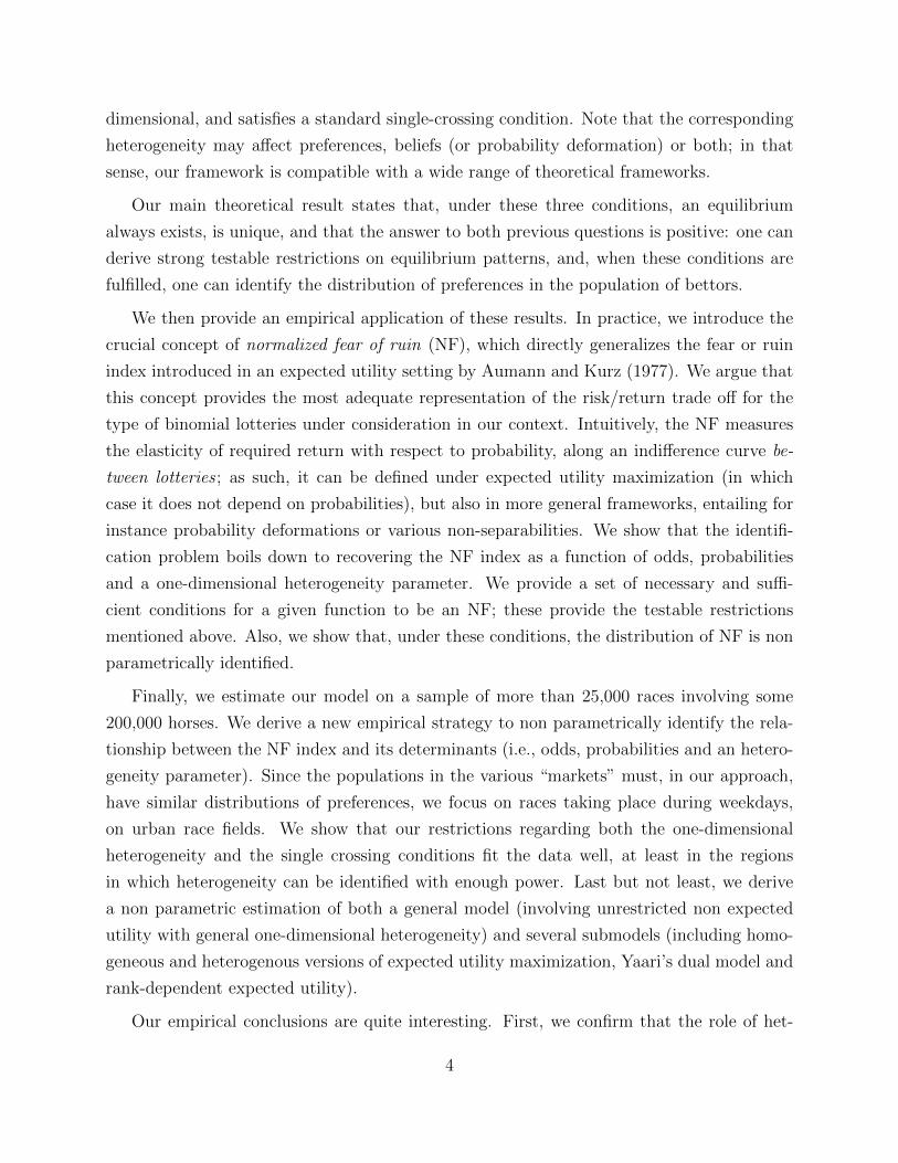
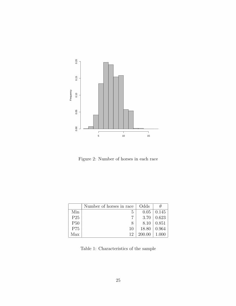
Figure 2 shows that almost all races have 5 to 12 horses. We eliminated the other 606

races. We also dropped 44 races in which one horse has odds larger than 200—a very rare

occurrence. That leaves us with a sample of 442,636 horses in 53,523 races.

Table 1 gives some descriptive statistics. The betting odds over horses in the data range

from extreme favorites (odds equaling 0.05, i.e., horses paying 5 cents on the dollar), to

extreme longshots (odds equaling 200, i.e., horses paying 200 dollars on the dollar). The

24

Fre

quen

cy

5 10 15

0.00

0.05

0.10

0.15

0.20

Figure 2: Number of horses in each race

Number of horses in race Odds θMin 5 0.05 0.145P25 7 3.70 0.623P50 8 8.10 0.851P75 10 18.80 0.964Max 12 200.00 1.000

Table 1: Characteristics of the sample

25

0 20 40 60 80 100

010

0020

0030

0040

00

R

Num

ber

of h

orse

s

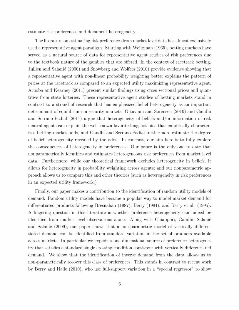
Figure 3: Distribution of odds, R ≤ 100

mean and median odds on a horse are 15.23 and 8.10 respectively: the distribution of odds

is highly skewed to the right. In our sample, 18.3% of horses have R ≥ 25 (odds of 20 or

more), 6.2% of horses have R ≥ 50, but only 0.7% have R ≥ 100. Also, the race take (t

in our notation) is heavily concentrated around 0.18: the 10th and 90th percentile of its

distribution are 0.165 and 0.209.

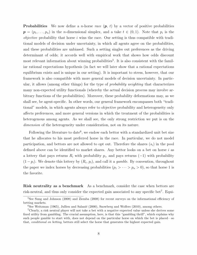
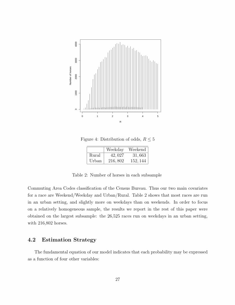
Figure 3 plots the raw distribution of odds up to R = 100. It seems fairly regular, with a

mode at odds of R = 2.5; but this is slightly misleading. Unlike market shares, odds are not a

continuously distributed variable: they are rounded at the track. We illustrate the rounding

mechanism on Figure 4: for odds below 4, odds are sometimes quoted in twentieths but

tenths are much more likely (e.g. R = 2.1 and R = 2.2 are much more likely than R = 2.15).

For longer odds the spacing of odds becomes coarser, but the same pattern still obtains (e.g.

R = 26.25 is much less likely than R = 26.0 or R = 26.5.) As we will explain later, this is

of no consequence except in so far as it constrains our choice of econometric methods.

We used two 0-1 covariates to see whether our results differed across subsamples. The

first covariate uses the date at which a race was run to separate weekday and weekend

races. To build our second covariate, we hand-collected the zip code of each racetrack, and

we used it to classify each track on an urban/rural scale, thanks to the 2000 Rural-Urban

26

0 1 2 3 4 5

010

0020

0030

0040

00

R

Num

ber

of h

orse

s

Figure 4: Distribution of odds, R ≤ 5

Weekday WeekendRural 42, 027 31, 663Urban 216, 802 152, 144

Table 2: Number of horses in each subsample

Commuting Area Codes classification of the Census Bureau. Thus our two main covariates

for a race are Weekend/Weekday and Urban/Rural. Table 2 shows that most races are run

in an urban setting, and slightly more on weekdays than on weekends. In order to focus

on a relatively homogeneous sample, the results we report in the rest of this paper were

obtained on the largest subsample: the 26,525 races run on weekdays in an urban setting,

with 216,802 horses.

4.2 Estimation Strategy

The fundamental equation of our model indicates that each probability may be expressed

as a function of four other variables:

27

∀ i < n pi+1(R) = G(Ri, pi(R), Ri+1, θi(R)) (11)

Remember that, in this relationship, the Rs and the θs are directly observable; our

estimation strategy aims at recovering both the probabilities and the function G. If the

function G was known (up to some parameters), then for each race these equations would

allow us to compute the winning probabilities, and the likelihood of the event that the

observed winner has indeed won the race. Maximizing the likelihood over all races then would

yield estimates of the parameters in G. This approach was adopted by Jullien and Salanie

(2000), in a setting where bettors were homogeneous, so that the indexes θi(R) disappears

from (11). Such an approach allows for the simultaneous estimation of probabilities and of

the parameters in G. Note that the resulting function p(R) is obtained without any a priori

restriction; but on the other hand, one has to adopt a parametric form for the function G,

thus imposing some restrictions to the class of preferences one may consider. For example,

Jullien and Salanie (2000) focused on parametric forms for some classes of EU (CARA,

HARA) and non-EU (RDEU, CPT) functions.

Since our main contribution bears on the identification of preferences, we shall instead

follow a two-step strategy, that allows us to recover preferences in a nonparametric way.

First, we estimate the function p(R) from the data on races just presented. This simple

step only involves choosing a flexible specification for p(R), which we do in the next section.

Once p(R) is recovered, we can then set up (11) as a nonparametric regression, that we

perform using Generalized Additive Models (GAMs); details are given in section 6.

A general advantage of our two-step strategy is that the estimation of the probabilities

does not rely on the theoretical framework described before; in this sense, it is fully agnostic

vis a vis the conceptual underpinnings. The testable restrictions implied by our general

framework—and by any of its more specialized versions—only bear on the function G, as

described by Proposition 3.

28

5 Estimating Probabilities

In order to estimate the probabilities pi(R), we resorted to a flexible, seminonparametric

approach. Without loss of generality, we can write

pi(R) =exp(Pi(R))∑nj=1 exp(Pj(R))

. (12)

for some functions P1, ..., Pn. Moreover, the dependence of each Pi on R is restricted by

the nature of the problem: it must depend on the odds (Rj)j 6=i in a symmetric way. To

incorporate this restriction, we specify the P functions as

Pi(R) = − log(Ri + 1) +K∑k=1

ak(Ri)Tk(R), (13)

where the Tk’s are symmetric functions of all odds R. To get an intuition for this expansion,

note that if the terms of the right-hand side sum were all zero, then each pi(R) would equal

the risk-neutral probability

pni (R) =

1

Ri + 1∑j

1

Rj + 1

of the benchmark case where individuals are risk-neutral. The purpose of the terms in the

sum is precisely to capture, in a flexible way, the deviations from the risk-neutral probability

reflecting the distribution of individual attitudes toward risk. In practice, we allowed for

K = 7 basis functions Tk: T1(R) ≡ 1; T2(R) =∑

i 1, which is the number of horses in that

race; and for k = 3, . . . , 7, Tk(R) =∑

i(1 + Ri)2−k. We also defined the terms ak(Ri) as

linear combinations of the first 15 orthogonal polynomials in 1/(1 +Ri).

To decide which terms should be included, we used two alternative model selection crite-

ria, the Akaike Information Criterion (AIC) and the Bayesian Information Criterion (BIC).

In both cases we started from the most parsimonious model with all ak’s zero and we used an

“add term, then drop term” stepwise strategy until we could not improve the model selection

criterion.

The estimated models are rather different (see Appendix 2 for precise results). The model

that yields the best value of the AIC has fourteen parameters: 8 on T1, 3 on T3, 2 on T4 and

1 on T5. Two of these fourteen parameters do not differ significantly from 0. As usual, the

29

BIC-selected model is more parsimonious: it selects two terms for T1, one for T3 and one for

T4. These four parameters very significantly differ from 0, with p < .001.

The finite precision of the estimates of the ak’s generates estimation errors on our esti-

mated probabilities pi(R), with accompanying standard errors which we denote σi. Since

our entire method relies on exploiting the deviations of these estimated probabilities from

the risk-neutral probabilities pni , we need these deviations to be large enough, relative to the

confidence bands for our estimated probabilities. In order to check that this is the case, we

ran nonparametric regressions of the ratios

pipni

andpi ± 1.96σi

pni

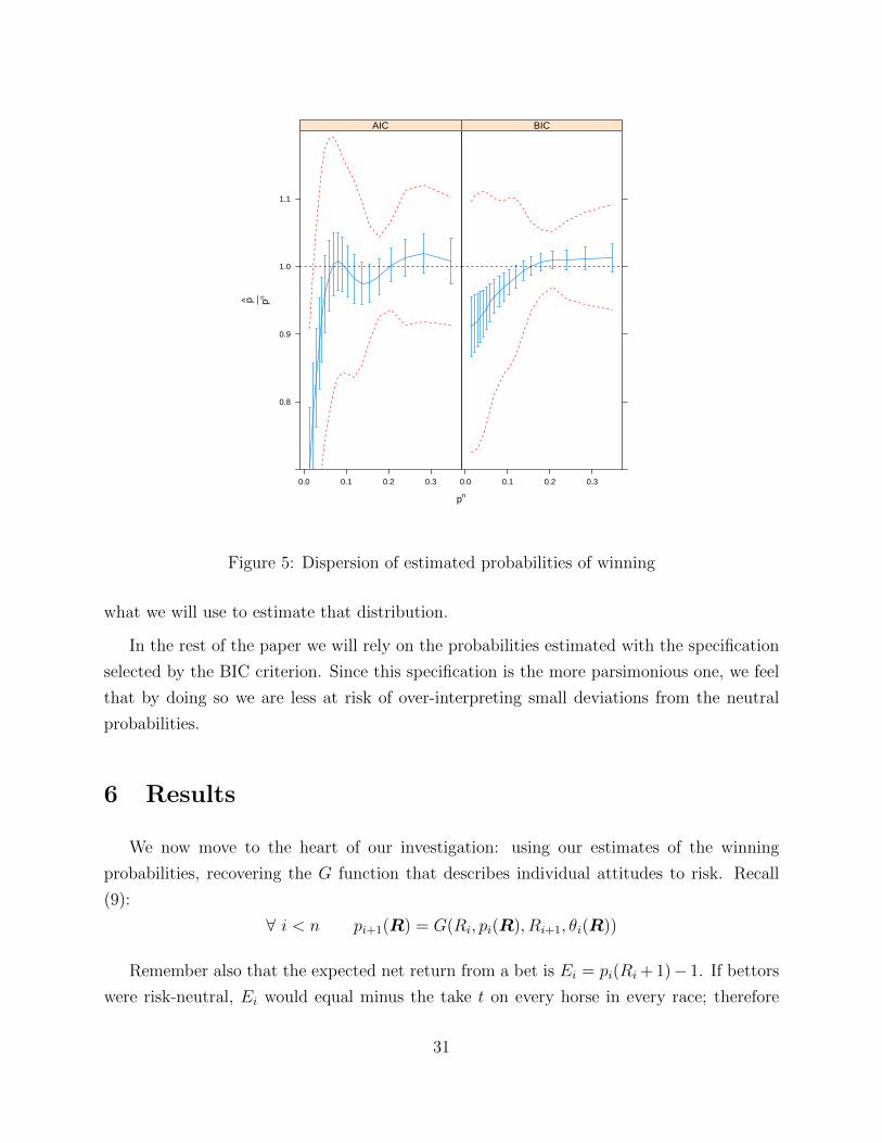
on the neutral probability pni ; and we plotted the result on figure 5. The central, blue curve

is the fitted value of pi/pni at the 5%, 10%, . . . , 95% quantiles of the distribution of pni ; and

the 95% confidence bars (also in blue) measure the estimation error.

To evaluate the dispersion of estimated probabilities pi relative to risk-neutral probabili-

ties pni , we ran a nonparametric regressions of pi on pni to obtain an estimate Ei = E (pi|pni ) ;

and a regression of the squared relative deviation(pi(R)− Ei

pni

)2

on pni to obtain a squared dispersion vi. Finally, we plotted two red dashed curves that

represent nonparametric fits of(Ei ± 1.96

√vi

)/pni . All of these nonparametric fits are

estimated very precisely, given the large sample size.

Figure 5 shows that while the AIC and BIC models give somewhat different pictures,

especially for outsiders (horses with longer odds, that is smaller neutral probabilities), in

both cases the dispersion of the estimated probabilities is much larger than their imprecision.

This is a reassuring finding.

The figure also retraces the ubiquitous finding that neutral probabilities overestimate

the probabilities of a win for outsiders—the favorite-longshot bias. However, the top and

bottom dashed curves clearly show that there is much more going on in the data: even with

the parsimonious estimates of the BIC model, our estimated probabilities of a win for many

outsiders are larger than the neutral probability. More generally, equilibrium odds do not

only reflect probabilities, but also the distribution of individual attitudes to risk; and this is

30

pn

p pn

0.8

0.9

1.0

1.1

0.0 0.1 0.2 0.3

AIC

0.0 0.1 0.2 0.3

BIC

Figure 5: Dispersion of estimated probabilities of winning

what we will use to estimate that distribution.

In the rest of the paper we will rely on the probabilities estimated with the specification

selected by the BIC criterion. Since this specification is the more parsimonious one, we feel

that by doing so we are less at risk of over-interpreting small deviations from the neutral

probabilities.

6 Results

We now move to the heart of our investigation: using our estimates of the winning

probabilities, recovering the G function that describes individual attitudes to risk. Recall

(9):

∀ i < n pi+1(R) = G(Ri, pi(R), Ri+1, θi(R))

Remember also that the expected net return from a bet is Ei = pi(Ri + 1)− 1. If bettors

were risk-neutral, Ei would equal minus the take t on every horse in every race; therefore

31

its variations in the data contain the information we need about preferences; in addition, by

construction, Ei + 1 = pi(Ri + 1) = (1 − t)pi/si measures how market shares deviate from

probabilities. Accordingly, we choose our dependent variable to be

ei(R) = log1 + Ei+1(R)

1 + Ei(R)= log

pi+1(R)(Ri+1 + 1)

pi(R)(Ri + 1),

and we run the regression

∀ i < n ei(R) = G(Ri, pi(R), Ri+1, θi(R)).

which is formally equivalent to our theoretical formulation above, with

G(R, p,R′, θ) ≡ pR + 1

R′ + 1exp

(G(R, p,R′, θ)

).

Note that if bettors were risk-neutral, the left-hand side variable ei(R) would be identically

zero (since t is constant within each race, risk-neutral betters would result in odds (plus one)

being inversely proportional to probabilities). Thus using ei allows us to focus on deviation

from risk-neutrality.

Since the above regression is valid for all horses but the last one in each race, from the

215,802 horses in our data we keep 190,277 observations; and after dropping the horses for

which Ri = Ri+1 which bring us no useful information, we end up with 185,409 horses.

Figure 6 gives the density of our LHS variable ei. Most of the distribution lies in the positive

region, reflecting the favorite-longshot bias: with higher expected returns on favorites, Ei is

usually larger than Ei+1. Still, 11% of the observations have a negative ei.

We estimated all of our regressions from this point using generalized additive models

(GAMs), which we describe in Appendix 3. Regressing ei on the four arguments of G gives

a generalized R2 of 0.878. Property (iv) of Proposition 3 requires an R2 of one, which is

clearly too much to ask. The very good fit of this first regression is a first indication that our

model explains a major share of the variations in the expected returns of bets—considering

that the R2 of a theory based on risk-neutral bettors would be zero in this regression.

We still need to check predictions (i) and (ii) of Proposition 3; prediction (iii) holds by

construction since pi = pi+1 whenever Ri = Ri+1. To examine predictions (i) and (ii), we

first compute G from the estimated G; then we simply evaluate numerically its first-order

derivatives with respect to all variables. The derivatives with respect to pi, Ri and Ri+1 have

32

0.00 0.05 0.10

010

2030

40

ei

Den

sity

Q1MedianQ3

Figure 6: Density of the LHS ei

the right signs in no less than 99.7% of the sample.

The derivative with respect to θ is more problematic. Property (i), which results from

our single crossing Assumption 3, implies that G should be decreasing in θ. In this first,

unrestricted regression 48% of the observations generate a positive derivative Gθ. This

sounds like a discouraging result. However, further analysis leads to qualify this negative

judgment. Indeed, the vast majority of these apparent violations of our theory come in

two regions of the space of gambles. One is the region θi < 0.4, in which most horses are

favorites in their race (i = 1). Remember that, by construction, θ1 = (1 − t)/(R1 + 1) for

favorites. Conditional on R1, any variation in θ1 must come from variations in track take

t. Since, as noticed above, there appears to be little variation in track take in the sample

(most takes being around 18%), the distribution of θ1 conditional on R1 is very concentrated,

which leaves little hope of estimating heterogeneous preferences in this region. This problem

relates to an obvious limitation of our study, already mentioned above: it is quite difficult

to estimate the bottom part of the θ distribution, since most of these agents systematically

behave in the same way—i.e., bet on the favorite.

The second region where violations of single crossing abound correspond to the other

end of the θ distribution (namely, θi > 0.95, corresponding to the least risk-averse 5% of

33

bettors.) Since our data is selected on horses and not on bettors, about 20% of the horses

in the regression sample have a θi > 0.95. As we will see, the derivative with respect to θ is

actually close to zero in this region.

We will document these facts in section 6.1; for now we ask the reader to bear with us.

Finally, we need to check property (ii)—that the marginal rate of substitution Gp/GR

is independent of R′. To do so, and in view of applying our study to various classes of

preferences, we first compute the normalized fear-of-ruin index

NF =p

R + 1

Gp

GR

at each observation13 (Ri, pi, Ri+1, θi). Then we regress NF on the three variables (Ri, pi, θi),

excluding Ri+1. Using GAM once more, we obtain a rather good fit since the R2 of this

regression is 0.827. This is reported on the first line of Table 3; since this corresponds to

the most general class of preferences that fit in our model, we take it as our estimate of

heterogeneous, non-expected utility (NEU) preferences.

Next, we can test a series of specific models, all of which are nested in the general

NEU specifications. Specifically, we consider an homogeneous version of NEU (whereby all

agents have the same attitude toward risk), and both a homogeneous and a heterogeneous

version of more restrictive frameworks: expected utility (EU), rank-dependent expected

utility (RDEU), and Yaari’s model. In all cases, the strategy is to explain NF by a subset

of variables and check how these restrictions affect the fit of the regression.

In practice, we first note that if preferences were homogeneous, then the representative

bettor with preferences V (R, p) would have to be indifferent between all horses in any given

race; and we would have

for all i < n, V (Ri, pi) = V (Ri+1, pi+1).

This is the equation used by Jullien-Salanie (2000) to estimate V . In order to accommodate

homogeneous preferences in our framework, we just drop the argument θi. In the NEU

regression, this amounts to letting NF only depend on R and p. In a similar way:

• heterogeneous expected utility (EU) obtains by excluding p, so that NF only depends

13We only kept the observations that had a value of NF between the P0.5 and P99.5 quantiles. Thisexcludes in particular the small number of observations for which GR or Gp have the wrong sign.

34

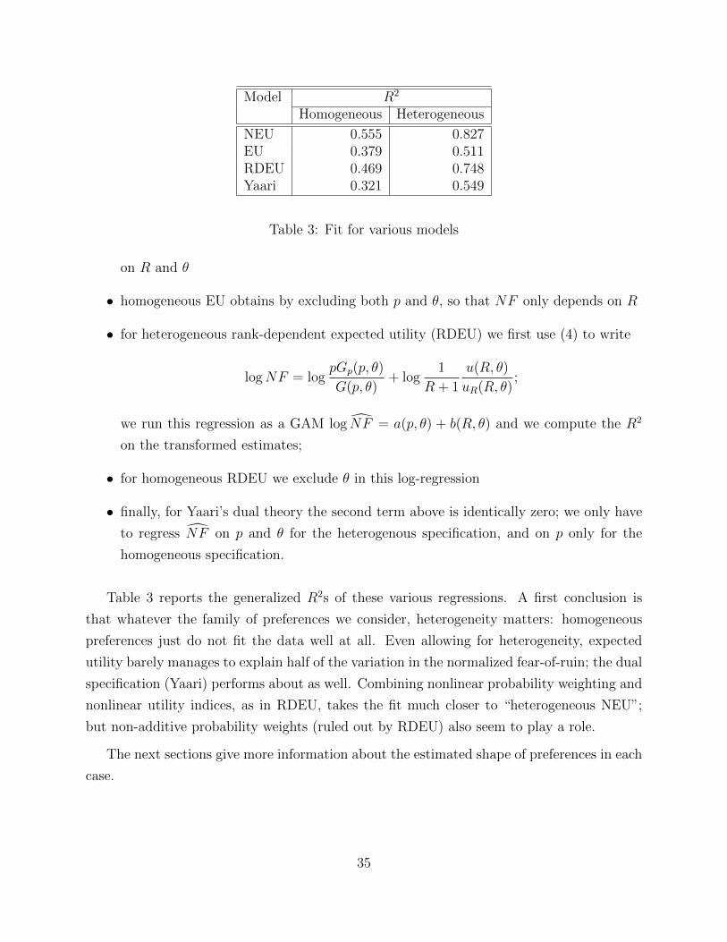
Model R2

Homogeneous Heterogeneous

NEU 0.555 0.827EU 0.379 0.511RDEU 0.469 0.748Yaari 0.321 0.549

Table 3: Fit for various models

on R and θ

• homogeneous EU obtains by excluding both p and θ, so that NF only depends on R

• for heterogeneous rank-dependent expected utility (RDEU) we first use (4) to write

logNF = logpGp(p, θ)

G(p, θ)+ log

1

R + 1

u(R, θ)

uR(R, θ);

we run this regression as a GAM log NF = a(p, θ) + b(R, θ) and we compute the R2

on the transformed estimates;

• for homogeneous RDEU we exclude θ in this log-regression

• finally, for Yaari’s dual theory the second term above is identically zero; we only have

to regress NF on p and θ for the heterogenous specification, and on p only for the

homogeneous specification.

Table 3 reports the generalized R2s of these various regressions. A first conclusion is

that whatever the family of preferences we consider, heterogeneity matters: homogeneous

preferences just do not fit the data well at all. Even allowing for heterogeneity, expected

utility barely manages to explain half of the variation in the normalized fear-of-ruin; the dual

specification (Yaari) performs about as well. Combining nonlinear probability weighting and

nonlinear utility indices, as in RDEU, takes the fit much closer to “heterogeneous NEU”;

but non-additive probability weights (ruled out by RDEU) also seem to play a role.

The next sections give more information about the estimated shape of preferences in each

case.

35

6.1 Expected utility

We start with the simplest version, based on expected utility. Figure 7 plots the estimated

normalized fear-of-ruin NF , as a function of odds R.

Homogeneous EU We may first consider the homogeneous EU case, represented by the

solid black curve; here, NF is a function of R only, and the circles indicate the nine deciles

D1-D9 of odds in the sample. The hypothetical representative bettor with EU preferences

would be risk-averse for low-return, safe bets, and risk-loving for all other bets.

Also represented on the Figure is the NF reconstructed from the EU preferences esti-

mated in Jullien and Salanie (2000) (“JS 2000” curve). Our estimates dramatically differ

from JS2000. The explanation for this discrepancy is that Jullien and Salanie took a para-

metric approach; they only considered HARA preferences, and found that within that class

a risk-loving CARA function fit their data best. Our nonparametric approach shows that

assuming a specific functional form is dangerous. For instance, HARA preferences imply a

“fanning out” patterns for NF : it increases in R if and only if it is larger than 1. But our

estimated NF is non monotonic and crosses the value 1: the data clearly rejects the HARA

framework.

Heterogenous EU The five Pxx solid curves plot NF (R, θ) as a function of R for the

heterogenous EU preferences that correspond to the quantiles P10, P25, P50, P75 and P90

of the distribution of θ in the sample. These quantiles are collected in Table 4. As Figure 8

makes clear, the distribution of θ in our sample is much more skewed to the right than the

distribution of θ among bettors, which is normalized to be uniform over [0, 1]. There are very

few small θ’s: in fact, since none of our races has more than 12 horses, we cannot observe

any θi below 1/12. More generally, our observations correspond to the edges of “market

share” intervals; and there are many more for outsiders, whose market share by definition is

smallest.

The distribution of odds R conditional on θ of course varies a great deal with θ. This

is the reason why the Pxx curves move to the right as the quantile of θ increases. As in

the homogeneous version, the circles indicate the D1-D9 deciles of the (now conditional)

distribution of odds. For the P10 curve the lower deciles of R are almost confounded; we

will return to this point below.

The Pxx curves in Figure 7 are very nicely ordered for odds lower than 15: holding

36

0 10 20 30 40

0.8

0.9

1.0

1.1

Odds

Nor

mal

ized

FO

R ●

●

● ● ●●

●●

●

●

●

●

●

●

●

●

●●●●●●●

●

●

●●●●●●●●●

●

●●

●●

● ●●

●

●●

●●

●●

● ●●

●●

● ● ● ● ● ●

Risk−neutralHomogeneousJS 2000P10(θ)P25(θ)P50(θ)P75(θ)P90(θ)

Figure 7: Homogeneous and heterogeneous EU

Quantile Value of θP10 0.375P25 0.600P50 0.821P75 0.938P90 0.976

Table 4: Quantiles of θi

37

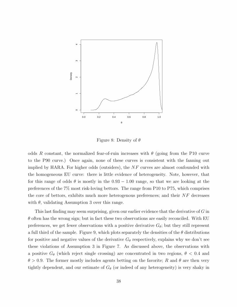
0.0 0.2 0.4 0.6 0.8 1.0

01

23

4

θ

Den

sity

Figure 8: Density of θ

odds R constant, the normalized fear-of-ruin increases with θ (going from the P10 curve

to the P90 curve.) Once again, none of these curves is consistent with the fanning out

implied by HARA. For higher odds (outsiders), the NF curves are almost confounded with

the homogeneous EU curve: there is little evidence of heterogeneity. Note, however, that

for this range of odds θ is mostly in the 0.93 − 1.00 range, so that we are looking at the

preferences of the 7% most risk-loving bettors. The range from P10 to P75, which comprises

the core of bettors, exhibits much more heterogenous preferences; and their NF decreases

with θ, validating Assumption 3 over this range.

This last finding may seem surprising, given our earlier evidence that the derivative ofG in

θ often has the wrong sign; but in fact these two observations are easily reconciled. With EU

preferences, we get fewer observations with a positive derivative Gθ; but they still represent

a full third of the sample. Figure 9, which plots separately the densities of the θ distributions

for positive and negative values of the derivative Gθ respectively, explains why we don’t see

these violations of Assumption 3 in Figure 7. As discussed above, the observations with

a positive Gθ (which reject single crossing) are concentrated in two regions, θ < 0.4 and

θ > 0.9. The former mostly includes agents betting on the favorite; R and θ are then very

tightly dependent, and our estimate of Gθ (or indeed of any heterogeneity) is very shaky in

38

0.0 0.2 0.4 0.6 0.8 1.0

01

23

45

6

θ

Den

sity

Negative derivativePositive derivative

Figure 9: Density of θ for subsamples by sign of Gθ

0.2 0.4 0.6 0.8 1.0

0.0

0.1

0.2

0.3

0.4

0.5

0.6

0.7

θ

1(1

+R

)

<−0.4[−0.4,−0.3][−0.3,−0.2][−0.2,−0.1][−0.1,0][0,0.1][0.1,0.2][0.2,0.3][0.3,0.4]>0.4

Figure 10: Density of θ for subsamples by value of Gθ

39

this region.

This interpretation is confirmed by Figure 10, which plots 1/(1+R) against θ (each point

represents an observation.) For θ < 0.4, most points group along a line of slope about 0.8,

which is the average value of (1− t); and violations are numerous in that region. Figure 10

also shows that in the other regions where positive derivatives Gθ are found, their value is

not very large. These are points in which G is basically flat in θ; they correspond to the part

in Figure 7 where the NF curves are almost confounded. With derivatives close to zero,

violations should be expected in that region, but they are not economically significant14.

Conversely, in the regions where there is enough variation in θ conditional on R to

estimate the derivative, negative derivatives predominate greatly except for the riskiest bets.

This is a satisfying finding: while Assumption 3 does not apply to all of our sample, it seems

to be a reasonable approximation.

Since the generalized additive models we use fit the data using flexible local functional

forms, the failure of Assumption 3 to hold everywhere should not contaminate our estimates

on the rest of the range. We checked this directly by fitting the models to the subsample of

horses such that θi > 0.4; our conclusions hardly changed.

6.2 Yaari’s dual model

Yaari’s 1987 model is a natural entry point into the very rich class of non-expected

utility models. Comparing the nonlinearity in odds V (p,R) = pu(R) of expected utility to

nonlinearity in probabilities V (p,R) = G(p)(R + 1) as in the dual theory nicely frames the

question in Snowberg and Wolfers (2010): what matters most, preferences or perceptions?

By comparing choice patterns across types of bets, they found that a representative “dual”

bettor explained the data better than a representative expected-utility bettor. In our richer

framework, we can benchmark these two theories using only win bets; and more importantly,

we can allow for one dimension of (single-crossing) heterogeneity in each of these two classes.

With a functional V (p,R, θ) = G(p, θ)(R+1), the normalized fear-of-ruin does not depend

on odds: it is simply

NF (p, θ) =pGp(p, θ)

G(p, θ),

the elasticity of the probability weighting function G with respect to p.

14The exception is bottom right corner in Figure 10, which corresponds to a small subpopulation of horseswith the longest of odds.

40

0.0 0.1 0.2 0.3 0.4

0.8

0.9

1.0

1.1

Probability

Nor

mal

ized

FO

R●

●●

●●

●●

● ● ● ● ● ● ●●

●

●

●

●

●

●

●●●●●●●

●● ● ● ● ● ●

●●

● ● ● ● ● ●●

●

●

●●●●●●●●

●

●●●●●●●●

●

Risk−neutralHomogeneousP10(θ)P25(θ)P50(θ)P75(θ)P90(θ)

Figure 11: Homogeneous and heterogeneous Yaari

As shown in Table 3, the dual theory fits the data about as well as expected utility.

Figure 11 plots the estimated NF as a function of p for the five usual quantiles of θ, in

addition to the estimate for the homogenous case in which G does not depend on θ. Just as

in Figure 7 for expected utility, the normalized fear-of-ruin is a nicely decreasing function of

θ on this graph, except for low probability bets (which were high odds bets in Figure 7) for

which preferences appear to be close to homogeneous. And as in the case of expected utility,

for low θ’s there is too little variation to estimate heterogeneity in preferences.

Since the normalized fear-of-ruin coincides with the elasticity of the probability weighting

function G, our estimates in both the homogeneous and the heterogeneous models suggest

that bettors tend to overestimate small probabilities (G is concave), while underestimating

larger ones (G becomes convex.) The point in which G has an elasticity of one is around a

probability of 0.3. Laboratory experiments concur that this is roughly the location of the

“crossing point” where G(p) = p. Since for a concave-then-convex function from [0, 1] to

[0, 1] the crossing point must be to the left of the unit-elasticity point, our results suggest a

crossing point somewhat smaller than in experimental data.

41

6.3 The general, non expected utility model

Our estimates of heterogeneous non-expected utility preferences are difficult to summa-

rize. Even testing for popular specifications like cumulative prospect theory,

V (p,R, θ) = G+(p, θ)u+(R, θ) +G−(1− p, θ)u−(θ)

is not easy without recurring to parametric specifications, which we have strived to avoid

in this paper. We will only discuss here our estimates for the homogenous non-expected

utility model, in which the normalized fear-of-ruin can depend arbitrarily on both odds R

and probability p. We found that the best way to summarize our results was to plot our

estimated NF as a function of R (as in Figure 7), with three curves15 that give p the values

of the three quartiles of the conditional distribution of p given R.

With expected utility, the three curves would be confounded since NF cannot depend on

p. Figure 12 therefore measures the quantitative importance of nonlinearity in probabilities

over and above nonlinearity in wealth within the homogeneous model. Note how the curves

cross for odds of about ten to one. For shorter odds (safer bets), the normalized fear-of-ruin

increases with p; and for longer odds (riskier bets) it decreases with p. It is easy to see that

if preferences were rank-dependent,

V (p,R) = G(p)u(R)

then this pattern suggests that the elasticity of G with respect to p is U-shaped, just as in

Figure 11 for dual expected utility. Once again, this points towards a probability weighting

function that is concave then convex, as one would expect from the experimental literature

(see e.g. Wakker (2010).) We find it very encouraging that results from such different

approaches, and from empirical specifications that are a priori so different converge towards

similar conclusions.

7 Concluding remarks

Our empirical work therefore lead to several conclusions. First, the most general model

(involving heterogeneous, non expected utility) fits the data quite well. This is an inter-

15Probabilities are closely linked to odds in the data; choosing unconditional quantiles of p as we did inFigures 7 and 11 would not be very enlightening.

42

0 10 20 30 40

0.8

0.9

1.0

1.1

Odds

Nor

mal

ized

FO

R●

● ●● ●

●●

●

●●

●●

● ●● ●

●

●

●

● ● ● ●

●●

●

●

Risk−neutralMedian p|RP25(p|R)P75(p|R)

Figure 12: Homogeneous NEU

esting message. Given our empirical strategy, estimated probabilities (the right hand side

of equation (11)) should in principle depend on the whole set of odds and market shares.

The theoretical restriction, which imposes that it only depends on four variables, thus has a

real bite. That the four variables distinguished by the theory explain 87.8% of the variance

is a very encouraging result. One goal of the paper was to show that a general theoretical

approach, based on general attitudes toward risk and allowing for heterogeneity among bet-

ters, could generate strong, testable implications on observed data. It does; moreover, these

restrictions seem to fit data fairly well.

A second conclusion is that the role of heterogeneity appears to be paramount. What-

ever the specific formulation, homogeneous models perform poorly, even when compared to

the simplest versions of the heterogeneous framework. The general message, then, is that

data stemming from the aggregation of (a large number of) individual behaviors cannot be

adequately summarized by the fiction of a representative agent. From that perspective, the

positive insight suggested by our approach is that the presence of heterogeneity does not

preclude identification, even in a non parametric framework.

Clearly, this conclusion must be somewhat qualified. Admittedly, the way heterogeneity is

introduced here is restrictive: it is one-dimensional and is required to satisfy a single crossing

43

property. These restrictions were introduced for identification purposes; non parametric

identification of models entailing multidimensional heterogeneity, or even one-dimensional

heterogeneity without single crossing, is a difficult problem well beyond the scope of the

present paper. It should be noted, however, that these restrictions are testable, and that

they seem to work quite well. Our rather parsimonious way of introducing heterogeneity

makes a very significant difference in the quality of the fit. Moreover, the single crossing

restriction can be checked from our estimates; and it is mostly consistent with them, at least

in regions where the heterogeneity of preferences can be identified.

A final lesson from our estimates is that the shape of individual preferences is quite

complex, and varies across individuals in a sophisticated way. Typically, the same individual

may be risk-averse for some bets and risk loving for others; and for any given bet, a fraction

of the population may behave in a risk averse way whereas another does not. In particular,

parametric models, which tend to impose strong restrictions on the behavior of key indicators

(e.g., fanning out of the normalized fear-of-ruin index), have to be used with great caution.

Our non parametric estimates clearly indicate that the most commonly used parametric

form (e.g., expected utility with HARA preferences) may grossly misrepresent the trade-off

between risk and return. In that sense, our main message is twofold: a model of decision

under risk involving general preferences and (one-dimensional) heterogeneity can indeed be

non parametrically identified from the sole equilibrium conditions; but the whole richness

of a nonparametric approach is needed to take into account the complexity of individual

decision processes, although some simpler versions seem to perform reasonably well.

References

A. Andrikogiannopoulou (2010), “Estimating Risk Preferences from a Large Panel of

Real-World Betting Choices”, Princeton University mimeo.

J. Andreoni and C. Sprenger (2010), “Uncertainty Equivalents: Testing the Limits of

the Independence Axiom”, mimeo UCSD.

S.B. Aruoba and M.S. Kearney (2010), “Do lottery gamblers love risk or overweight

small odds?”, University of Maryland working paper.

R.J. Aumann and M. Kurz (1977), “Power and taxes”, Econometrica, vol. 45, 1137-

1161.

L. Barseghyan, F. Molinari, T. O’Donoghue and J.C. Teitelbaum (2011), “The

44

nature of risk preferences: evidence from insurance choices”, SSRN 1646520.

R. B. Barsky, F. T. Juster, M. S. Kimball and M. D. Shapiro (1997), “Preference

Parameters and Behavioral Heterogeneity: An Experimental Approach in the Health and

Retirement Study”, Quarterly Journal of Economics, Vol. 112, No. 2, May, 537-579.

R.M.W.J. Beetsma and P.C. Schotman (2001), “Measuring Risk Attitudes in a Nat-

ural Experiment: Data from the Television Game Show Lingo”, Economic Journal, Royal

Economic Society, vol. 111(474), 821-48, October.

S. Berry (1994), “Estimating Discrete Choice Models of Product Differentiation”, RAND

Journal of Economics, 25, 242-262.

S. Berry, J. Levinsohn and A. Pakes (1995), “Automobile Prices in Market Equilib-

rium”, Econometrica, 60(4), 889-917. Reprinted in Empirical Industrial Organization, vol.

I, P. Joskow and M. Waterson, eds., Edward Elgar Press, 2004.

S. Berry and P. Haile (2010), “Identification in Differentiated Product Markets using

Market Level Data”, Yale University discussion paper.

S. Berry, A. Gandhi, and P. Haile (2010), “Connected Substitutes and Invertibility of

Demand”, Yale University discussion paper.

S. Bonhomme, P.A. Chiappori, H. Yamada and R. Townsend (2012), “Sharing

Wage Risk”, mimeo, MIT.

H. Bonin, T. Dohmen, A. Falk, D. Huffman and U. Sunde (2007), “Cross-Sectional

Earnings Risk and Occupational Sorting: The Role of Risk Attitudes”, Labour Economics,

14, 926–937.

D.J. Brown and R.L. Matzkin (1996), “Testable restrictions on the equilibrium mani-

fold”, Econometrica, 64, 1249–1262.

A. Bruhin, H. Fehr-Duda, and T. Epper (2010), “Risk and Rationality: Uncovering

Heterogeneity in Probability Distortion”, Econometrica, 78: 1375–1412.

P.A. Chiappori, I. Ekeland, F. Kubler and H. Polemarchakis (2002), “The Iden-

tification of Preferences from Equilibrium Prices under Uncertainty”, Journal of Economic

Theory, 102, 403–420.

P.A. Chiappori, I. Ekeland, F. Kubler and H. Polemarchakis (2004), “Testable

Implications of General Equilibrium Theory: A Differentiable Approach”, Journal of Math-

ematical Economics, Special issue in honor of Werner Hildenbrand, 40, 105–119.

45

P.A. Chiappori, A. Gandhi, B. Salanie and F. Salanie (2009), “Identifying Prefer-

ences under Risk from Discrete Choices”, American Economic Review, Papers & Proceedings,

99, 356–362.

P.A. Chiappori and M. Paiella (2011), “Relative Risk-Aversion is constant: evidence

from panel data”, Journal of the European Economic Association, 9, 1021–1052.

P.A. Chiappori, K. Samphantharak, S. Schulhofer-Wohl and R. M. Townsend

(2012), “Heterogeneity and Risk Sharing in Thai Villages”, mimeo, MIT.

A. Cohen and L. Einav (1997), “Estimating risk preferences from deductible choice”,

American Economic Review, vol. 97, 745–788.

T. Dohmen, A. Falk, D. Huffman, U. Sunde, J. Schupp, and G. Wagner (2011),

“Individual Risk Attitudes: Measurement, Determinants and Behavioral Consequences”,

Journal of the European Economic Association, 9, 522–550.

J. Foncel and N. Treich (2005), “Fear of ruin”, Journal of Risk and Uncertainty 31,

289-300.

A. Gandhi (2006), “Rational Expectations at the Racetrack: Testing Expected Utility

Using Prediction Market Prices”, Chicago University working paper.

A. Gandhi and R. Serrano-Padial (2011), “The aggregate effects of idiosyncratic hetero-

geneity: evidence from an Arrow-Debreu securities market”, University of Maryland working

paper.

E. Gautier and Y. Kitamura (2012), “Nonparametric Estimation in Random Coeffi-

cients Binary Choice Models”, forthcoming in Econometrica.

C. Gollier and B. Salanie (2006), “Individual decisions under risk, risk sharing and asset

prices with regret”, mimeo.

L. Guiso and M. Paiella (2006), “The Role of Risk-aversion in Predicting Individual

Behavior”, in Competitive Failures in Insurance Markets: Theory and Policy Implications,

P.-A. Chiappori and C. Gollier eds, MIT Press and CESifo, 213–250.

L.P. Hansen (2007), “Beliefs, Doubts and Learning: Valuing Macroeconomic Risk”, Amer-

ican Economic Association Papers and Proceedings, 97, 1-30.

L.P. Hansen and T. Sargent (2007), Robustness, Princeton University Press.

T. Hastie and R. Tibshirani (1986): “Generalized additive models” (with discussion),

Statistical Science, 1, 297–318.

46

T. Hastie, R. Tibshirani and J. Friedman (2001), The Elements of Statistical Learning,

Springer.

B. Jullien and B. Salanie (2000), “Estimating Preferences under Risk: The Case of

Racetrack Bettors”, Journal of Political Economy, 108, 503–530.

B. Koszegi and M. Rabin (2007), “Reference-dependent Risk-Attitudes”, American

Economic Review, 97, 1047–1073.

M. Ottaviani and P. Sorensen (2010), “Noise, Information and the Favorite-Longshot

Bias in Parimutuel Predictions”,American Economic Journal: Microeconomics, 2, 58-85.

E. Snowberg and J. Wolfers (2010), “Explaining the Favorite-Longshot Bias: Is It

Risk-Love or Misperceptions?”, Journal of Political Economy, 118, 723-746.

M. Sung and J, Johnson (2008), “Semi-Strong From Efficiency in Horse Race Betting”,

in Handbook of Sports and Lottery Markets, D. Hausch and W. Ziemba eds, North Holland.

J. Sydnor (2010), “(Over)Insuring Modest Risks”, American Economic Journal: Applied

Economics, 2, 177–199.

P. Wakker (2010), Prospect Theory: For Risk and Ambiguity, Cambridge University Press.

M. Weitzman (1965), “Utility Analysis and Group Behavior: An Empirical Study”, Jour-

nal of Political Economy 73, 18–26.

S. Wood (2006), Generalized Additive Models: An Introduction with R, Chapman and

Hall/CRC Press.

S. Wood (2008), “Fast Stable Direct Fitting and Smoothness Selection for Generalized

Additive Models”, Journal of the Royal Statistical Society B, 70, 495–518.

M. Yaari (1987), “The dual theory of choice under risk”, Econometrica, 55, 95-115.

W. Ziemba (2008), “Efficiency of Betting Markets”, in Handbook of Sports and Lottery

Markets, D. Hausch and W. Ziemba eds, North Holland.

47

Appendix 1: Proofs

Proof of Lemma 2: from the single-crossing assumption, the set of agents that strictly

prefer horse i to horse j > i is an interval containing 0. Similarly, the set of agents that

strictly prefer horse i to horse j < i is an interval containing 1. Therefore the set of agents

that strictly prefer horse i to all other horses is an interval. The single-crossing assumption

also implies that these intervals are ranked by increasing i; and that the set of agents indif-

ferent between horse i and horse (i+ 1) is a singleton. Q.E.D.

Proof of Proposition 1: from Definition 1, given a race (p, t) we have to find a family R

such that, for all i < n,

V

(pi, Ri, (1− t)

∑j≤i

1

Rj + 1

)= V

(pi+1, Ri+1, (1− t)

∑j≤i

1

Rj + 1

)

From the first-order stochastic dominance assumption, the right-hand-side is increasing

with Ri+1, and is strictly below the left-hand-side at Ri+1 = Ri. Moreover Assumption 2 im-

plies that the right-hand-side is strictly above the left-hand-side for Ri+1 high enough. Thus

this equality defines a unique Ri+1, such that Ri+1 > Ri. The single-crossing assumption then

ensures that the difference between the right-hand-side and the left-hand-side is growing in θ

at the right of (1−t)∑

j≤i1

Rj+1. Since in addition VR > 0, this proves that Ri+1 is an increas-

ing function of Ri, and a non-decreasing function of each Rj, j < i. Iterating this remark, we

get that each Ri+1 is an increasing function of R1. Replacing in (2), we get an equation in

R1 which has at most one solution. Existence follows from the fact that (R1, . . . , Rn) forms

an increasing sequence, so that by setting R1 high enough we get 1/(1− t) >∑

j 1/(1 +Rj);

and from the fact that when R1 goes to −t we get 1/(1− t) <∑

j 1/(1 +Rj). Q.E.D.

Proof of Proposition 2: If we know the odds, then we know the take and the market

shares, from (1) and (2); and we also know the indexes (θj(R)) of marginal bettors, from

(6). There only remains to find a family p solution to the system

∀ i < n V (Ri, pi, θi) = V (Ri+1, pi+1, θi)

Let us focus on positive probabilities. From the first-order stochastic dominance assump-

tion, the right-hand-side is increasing with pi+1, and is strictly above the left-hand-side at

48

pi+1 = pi. From Assumption 1, it is also strictly below the left-hand-side when pi+1 goes

to zero: therefore pi+1 is uniquely defined, and pi+1 < pi. Moreover pi+1 is an increasing

function of pi, and thus of p1. Finally p1 is uniquely determined by p1 +∑

i<n pi+1 = 1

(existence follows from checking the cases p1 → 0 and p1 = 1). Q.E.D.

Appendix 2: estimating probabilities

Recall that we estimate probabilities in a flexible way (see section 5), on a dataset with

216,802 horses and 26,525 races. In the AIC case (Table 5), the log-likelihood is maximized

at (−91, 989.28), for a model that retains fourteen parameters: 8 on T1, 3 on T3, 2 on T4

and 1 on T5. Two of these fourteen parameters do not differ significantly from 0. We list

the parameter values below, but they are hard to interpret given the flexible specification we

used, and the fact that we recentered and rescaled the polynomial terms during estimation.

Names Estimates Standard Errors (Student)T1: 1 0.137 0.023 (6.0)T1: 2 0.073 0.036 (2.0)T1: 3 0.180 0.035 (5.2)T1: 4 0.017 0.017 (1.0)T1: 5 0.049 0.009 (5.2)T1: 6 −0.040 0.010 (4.2)T1: 7 0.038 0.008 (5.0)T1: 8 −0.011 0.007 (1.5)T3: 1 −0.079 0.017 (4.5)T3: 2 0.049 0.023 (2.2)T3: 3 0.057 0.014 (4.0)T4: 1 0.379 0.072 (5.3)T4: 2 −0.165 0.043 (3.8)T5: −0.394 0.090 (4.4)

Table 5: Coefficient estimates in the AIC model

As usual, the BIC-selected model (Table 6) is more parsimonious: it selects two terms

for T1, one for T3 and one for T4. These four parameters very significantly differ from 0, with

p < .001. Now the log-likelihood is maximized at (−92, 072.04).

49

Names Estimates Standard Errors (Student)T1: 1 0.025 0.007 (3.5)T1: 2 −0.036 0.011 (3.3)T3: 1 −0.074 0.010 (7.5)T4: 1 0.072 0.014 (5.2)

Table 6: Coefficient estimates in the BIC model

Appendix 3: Generalized Additive Models

Generalized additive models (GAM) were introduced by Hastie and Tibshirani (1986).

They model a variable yi by assuming that its distribution around its mean belongs to the

exponential family and by modeling the mean as a sum of smooth functions of subvectors of

the covariates (Xi). More precisely, one writes

g(Eyi) =J∑j=1

fj(Xji ) (14)

where g is a user-defined smooth, monotonic link function, eachXji is a user-defined subvector

of Xi, and the fj are to be estimated; and the user also chooses the distribution of the error

term (yi − Eyi) within the exponential family.

There are two main reasons why GAMs are attractive for our purpose:

• unlike kernel-based methods, they do not require that the covariates have continuous

support; in our case Xi includes odds Ri, which have discrete support;

• restrictions on the form of utility functions often translate directly into restrictions on

the components Xji that may appear on the RHS of (14).

To estimate our GAM models, we use the methods described by Wood (2006); we use

his implementation in the mgcv package of R, which incorporates the improved algorithm

of Wood (2008). Dropping the i index and assuming that the link function g is simply the

identity, the GAM in (1) is

E(y|x) =J∑j=1

fj(xj)

with the xj’s subvectors of x. Modeling starts by choosing a rich family of basis functions

(typically splines) (bjk) for k = 1, . . . , Kj, with a maximal order Kj chosen large enough.

50

We then represent fj(xj) withKj∑k=1

βjkbjk(xj).

This gives a linear model

E(y|x) = Xβ;

but fitting it by OLS would typically overfit; to avoid overfitting, we penalize “wiggliness”

by choosing smoothing parameters (λj). The algorithm then chooses β to minimize∑i

(yi −Xiβ)2 +∑j

λjwj(β),

with wj(β) approximating∫f ′′j (x; β)2dx.

For given λ this gives us an estimator β(λ); we still need to pick the smoothing parameters

λ. The generalized Akaike Information Criterion would choose λ to minimize∑i

(yi −Xiβ(λ))2 + 2τ(λ)σ2,

with σ2 an estimate of V (y|x), and τ the number of “effective degrees of freedom”, which is

the trace of the influence matrix16.

Using the generalized AIC may work badly because it tends to overparameterize, creating

convergence difficulties and numerical instabilities, especially if some covariates are close to

nonlinear functions of others—this is called “concurvity” in this literature. Wood prefers to

choose λ to minimize ∑i

(yi −Xiβ(λ))2(

1 + 2τ(λ)

n− τ(λ)

),

which he justifies in his 2008 paper by a Taylor expansion of the (theoretically best but

computationally demanding) cross-validation criterion. Since for a well-specified model we

should have ∑i

(yi −Xiβ(λ))2 ' nσ2,

the criterion used by Wood leads to somewhat more parsimonious specifications than if the

generalized AIC was used. Finally, the generalized R2’s cited in the text are defined in the

16For a linear model this would be just the number of covariates; for a fully nonparametric model it wouldbe the number of observations. It is not an integer for GAMs.

51

obvious way, as the ratio

1− EV (y|x)

V y.

52