Frequency Domain Normal Map Filtering

Charles Han Bo Sun Ravi Ramamoorthi Eitan Grinspun

Columbia University∗

Abstract

Filtering is critical for representing detail, such as color textures ornormal maps, across a variety of scales. While MIP-mapping tex-ture maps is commonplace, accurate normal map filtering remainsa challenging problem because of nonlinearities in shading—wecannot simply average nearby surface normals. In this paper, weshow analytically that normal map filtering can be formalized asa spherical convolution of the normal distribution function (NDF)and the BRDF, for a large class of common BRDFs such as Lamber-tian, microfacet and factored measurements. This theoretical resultexplains many previous filtering techniques as special cases, andleads to a generalization to a broader class of measured and ana-lytic BRDFs. Our practical algorithms leverage a significant bodyof work that has studied lighting-BRDF convolution. We show howspherical harmonics can be used to filter the NDF for Lambertianand low-frequency specular BRDFs, while spherical von Mises-Fisher distributions can be used for high-frequency materials.

1 Introduction

Representing surface detail at a variety of scales requires good fil-tering algorithms. For texture mapping, there has been consider-able effort at developing and analyzing filtering methods [Heck-bert 1989]. A common, linear approach to reduce aliasing is MIP-mapping [Williams 1983]. Normal mapping (also known as bumpmapping [Blinn 1978] or normal perturbation), a simple and widelyused analogue to color texture mapping, specifies the surface nor-mal at each texel. Unfortunately, normal map filtering is very diffi-cult because shading is not linear in the normal.

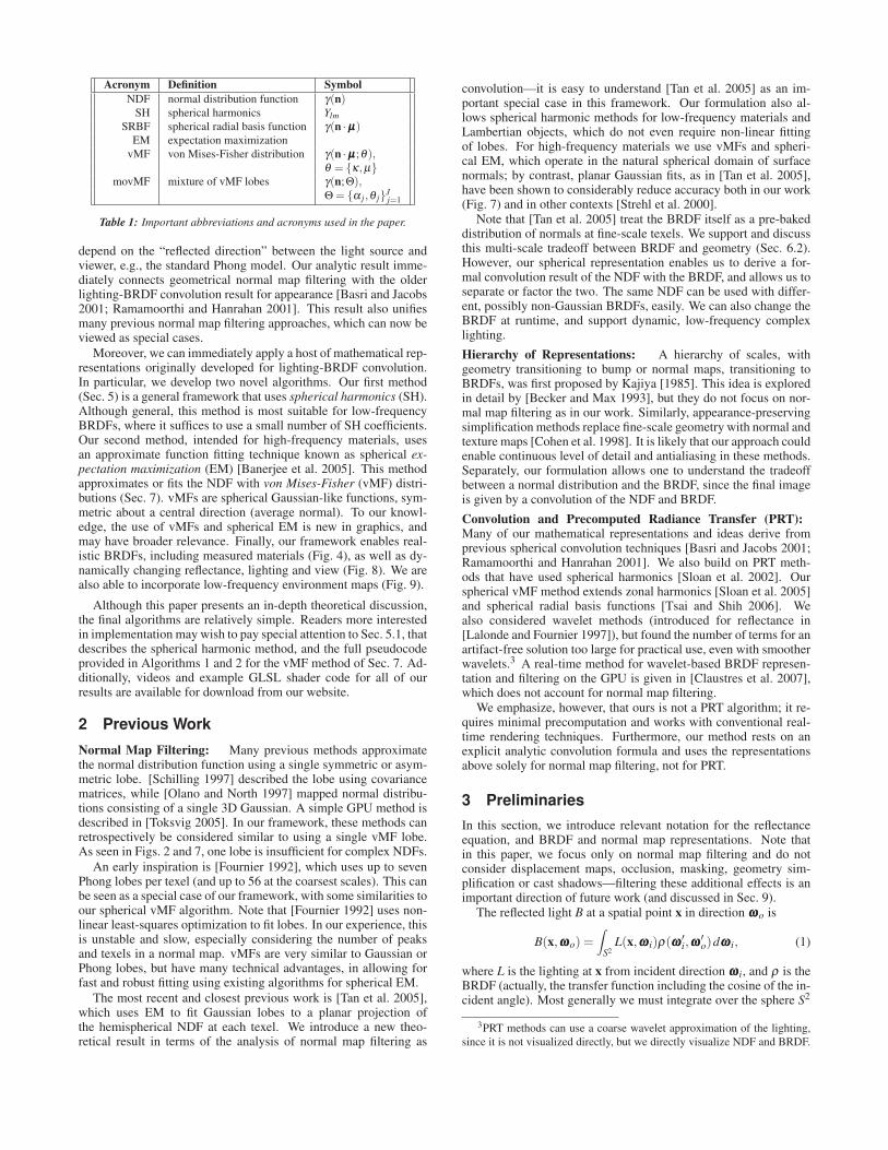
For example, consider the simple V-groove surface geometry inFig. 1a. In a closeup, this spans two pixels, each of which hasdistinct normals (b). As we zoom out (c), the average normal of thetwo sides (e) corresponds simply to a flat surface, where the shadingis likely very different. By contrast, our method preserves the fullnormal distribution (d) in the spirit of [Fournier 1992], and showshow to convolve it with the BRDF (f) to get an accurate result.

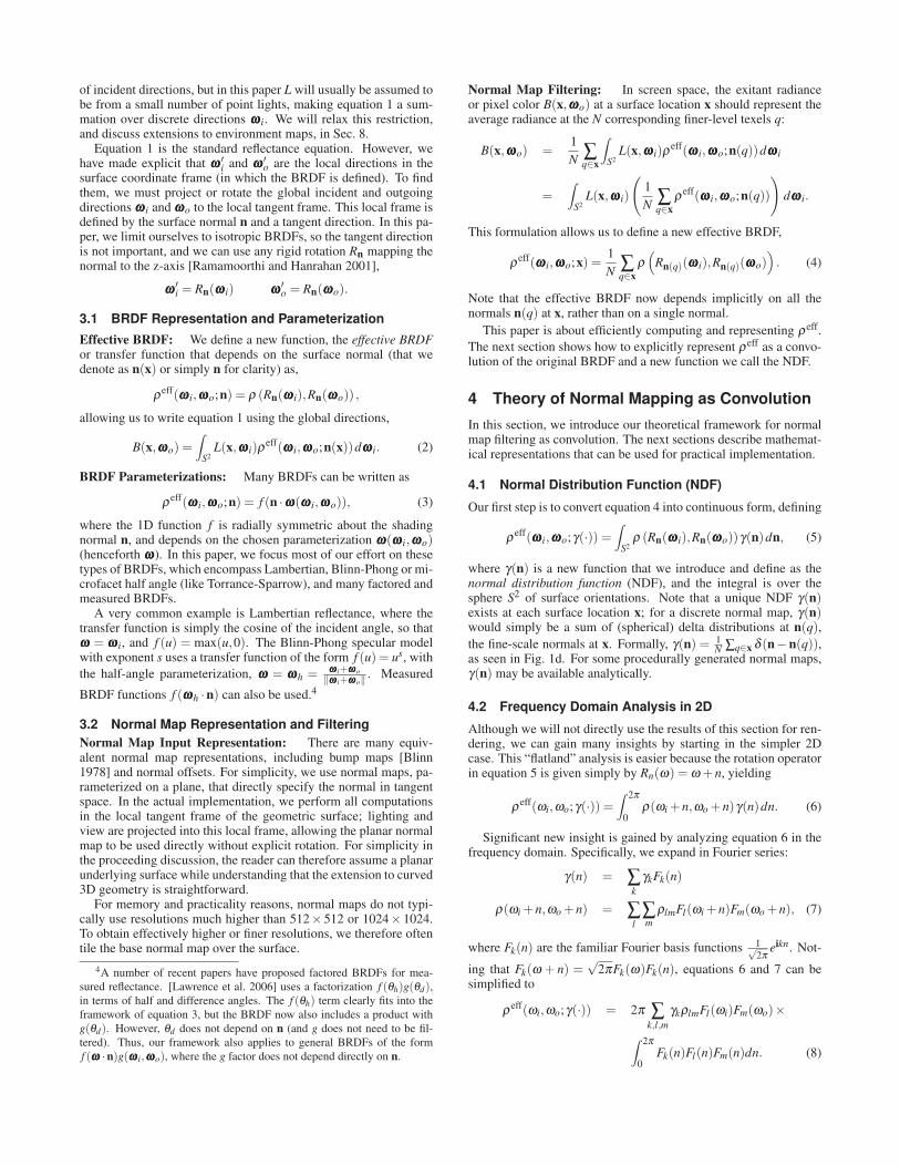
A more complex example is Fig. 2, which compares our methodwith “ground truth”1, standard MIP-mapping of normals, and therecent normal map filtering technique of [Toksvig 2005]. At closerange (top row), minimal filtering is required and all methods per-form identically. However, as we zoom out (middle and especiallybottom rows), we quickly obtain radically different results.

It has long been known qualitatively that antialiasing involvesconvolution of the input signal (here, the distribution of surface

∗{charhan,bosun,ravir,eitan}@cs.columbia.edu

URL: http://www.cs.columbia.edu/cg/normalmap1“Ground truth” images are obtained using jittered supersampling (on

the order of hundreds of samples per pixel) and unfiltered normal maps.

zoomed in

zoomed out

(a) V-groove

(e) standard

(d) NDF

(c) V-groove

(b)

NDF BRDF effective

BRDF

convolution(f)

Figure 1: Consider a simple V-groove. Initially in closeup (a), each face is

a single pixel. As we zoom out, and average into a single pixel (c), standard

MIP-mapping averages the normal to an effectively flat surface (e). How-

ever, our method uses the full normal distribution function or NDF (d), that

preserves the original normals. This NDF can be linearly convolved with

the BRDF (f) to obtain an effective BRDF, accurate for shading.

Figure 2: Top: Closeup of the base normal map; all other methods

are identical at this scale and are not shown. Schematic (a) and dif-

fusely shaded (b) views are provided to aid in comparison/visualization.

Middle: When we zoom out, differences emerge between our (6-lobe) spher-

ical vMF method, the Toksvig approach (rightmost), and normalized MIP-

mapping. (Unnormalized MIP-mapping of normals produces an essentially

black image.) Bottom: Zooming out even further, our method is clearly

more accurate than Toksvig’s model, and compares favorably with ground

truth. (The reader may zoom into the PDF to compare images.)

normals) and an appropriate low-pass filter. Our most importantcontribution is theoretical, formalizing these ideas and developinga comprehensive framework for normal map filtering.

In Sec. 4, we derive an analytic formula, showing that filteringcan be written as a spherical convolution of the BRDF of the ma-terial with a function we define as the normal distribution function(NDF)2 of the texel. This mathematical form holds for a large classof common BRDFs including Lambertian, Blinn-Phong, microfacetmodels like Torrance-Sparrow, and many measured BRDFs. How-ever, the convolution does not apply exactly to BRDF models that

2We define the NDF as a weighted mapping of surface normals onto the

unit sphere; more formally, it is the extended Gaussian Image [Horn 1984]

of the geometry within a texel.

Acronym Definition Symbol

NDF normal distribution function γ(n)SH spherical harmonics Ylm

SRBF spherical radial basis function γ(n ·µµµ)EM expectation maximization

vMF von Mises-Fisher distribution γ(n ·µµµ ;θ),θ = {κ,µ}

movMF mixture of vMF lobes γ(n;Θ),Θ = {α j,θ j}J

j=1

Table 1: Important abbreviations and acronyms used in the paper.

depend on the “reflected direction” between the light source andviewer, e.g., the standard Phong model. Our analytic result imme-diately connects geometrical normal map filtering with the olderlighting-BRDF convolution result for appearance [Basri and Jacobs2001; Ramamoorthi and Hanrahan 2001]. This result also unifiesmany previous normal map filtering approaches, which can now beviewed as special cases.

Moreover, we can immediately apply a host of mathematical rep-resentations originally developed for lighting-BRDF convolution.In particular, we develop two novel algorithms. Our first method(Sec. 5) is a general framework that uses spherical harmonics (SH).Although general, this method is most suitable for low-frequencyBRDFs, where it suffices to use a small number of SH coefficients.Our second method, intended for high-frequency materials, usesan approximate function fitting technique known as spherical ex-pectation maximization (EM) [Banerjee et al. 2005]. This methodapproximates or fits the NDF with von Mises-Fisher (vMF) distri-butions (Sec. 7). vMFs are spherical Gaussian-like functions, sym-metric about a central direction (average normal). To our knowl-edge, the use of vMFs and spherical EM is new in graphics, andmay have broader relevance. Finally, our framework enables real-istic BRDFs, including measured materials (Fig. 4), as well as dy-namically changing reflectance, lighting and view (Fig. 8). We arealso able to incorporate low-frequency environment maps (Fig. 9).

Although this paper presents an in-depth theoretical discussion,the final algorithms are relatively simple. Readers more interestedin implementation may wish to pay special attention to Sec. 5.1, thatdescribes the spherical harmonic method, and the full pseudocodeprovided in Algorithms 1 and 2 for the vMF method of Sec. 7. Ad-ditionally, videos and example GLSL shader code for all of ourresults are available for download from our website.

2 Previous Work

Normal Map Filtering: Many previous methods approximatethe normal distribution function using a single symmetric or asym-metric lobe. [Schilling 1997] described the lobe using covariancematrices, while [Olano and North 1997] mapped normal distribu-tions consisting of a single 3D Gaussian. A simple GPU method isdescribed in [Toksvig 2005]. In our framework, these methods canretrospectively be considered similar to using a single vMF lobe.As seen in Figs. 2 and 7, one lobe is insufficient for complex NDFs.

An early inspiration is [Fournier 1992], which uses up to sevenPhong lobes per texel (and up to 56 at the coarsest scales). This canbe seen as a special case of our framework, with some similarities toour spherical vMF algorithm. Note that [Fournier 1992] uses non-linear least-squares optimization to fit lobes. In our experience, thisis unstable and slow, especially considering the number of peaksand texels in a normal map. vMFs are very similar to Gaussian orPhong lobes, but have many technical advantages, in allowing forfast and robust fitting using existing algorithms for spherical EM.

The most recent and closest previous work is [Tan et al. 2005],which uses EM to fit Gaussian lobes to a planar projection ofthe hemispherical NDF at each texel. We introduce a new theo-retical result in terms of the analysis of normal map filtering as

convolution—it is easy to understand [Tan et al. 2005] as an im-portant special case in this framework. Our formulation also al-lows spherical harmonic methods for low-frequency materials andLambertian objects, which do not even require non-linear fittingof lobes. For high-frequency materials we use vMFs and spheri-cal EM, which operate in the natural spherical domain of surfacenormals; by contrast, planar Gaussian fits, as in [Tan et al. 2005],have been shown to considerably reduce accuracy both in our work(Fig. 7) and in other contexts [Strehl et al. 2000].

Note that [Tan et al. 2005] treat the BRDF itself as a pre-bakeddistribution of normals at fine-scale texels. We support and discussthis multi-scale tradeoff between BRDF and geometry (Sec. 6.2).However, our spherical representation enables us to derive a for-mal convolution result of the NDF with the BRDF, and allows us toseparate or factor the two. The same NDF can be used with differ-ent, possibly non-Gaussian BRDFs, easily. We can also change theBRDF at runtime, and support dynamic, low-frequency complexlighting.

Hierarchy of Representations: A hierarchy of scales, withgeometry transitioning to bump or normal maps, transitioning toBRDFs, was first proposed by Kajiya [1985]. This idea is exploredin detail by [Becker and Max 1993], but they do not focus on nor-mal map filtering as in our work. Similarly, appearance-preservingsimplification methods replace fine-scale geometry with normal andtexture maps [Cohen et al. 1998]. It is likely that our approach couldenable continuous level of detail and antialiasing in these methods.Separately, our formulation allows one to understand the tradeoffbetween a normal distribution and the BRDF, since the final imageis given by a convolution of the NDF and BRDF.

Convolution and Precomputed Radiance Transfer (PRT):Many of our mathematical representations and ideas derive fromprevious spherical convolution techniques [Basri and Jacobs 2001;Ramamoorthi and Hanrahan 2001]. We also build on PRT meth-ods that have used spherical harmonics [Sloan et al. 2002]. Ourspherical vMF method extends zonal harmonics [Sloan et al. 2005]and spherical radial basis functions [Tsai and Shih 2006]. Wealso considered wavelet methods (introduced for reflectance in[Lalonde and Fournier 1997]), but found the number of terms for anartifact-free solution too large for practical use, even with smootherwavelets.3 A real-time method for wavelet-based BRDF represen-tation and filtering on the GPU is given in [Claustres et al. 2007],which does not account for normal map filtering.

We emphasize, however, that ours is not a PRT algorithm; it re-quires minimal precomputation and works with conventional real-time rendering techniques. Furthermore, our method rests on anexplicit analytic convolution formula and uses the representationsabove solely for normal map filtering, not for PRT.

3 Preliminaries

In this section, we introduce relevant notation for the reflectanceequation, and BRDF and normal map representations. Note thatin this paper, we focus only on normal map filtering and do notconsider displacement maps, occlusion, masking, geometry sim-plification or cast shadows—filtering these additional effects is animportant direction of future work (and discussed in Sec. 9).

The reflected light B at a spatial point x in direction ωωωo is

B(x,ωωωo) =∫

S2L(x,ωωω i)ρ(ωωω ′i,ωωω

′o)dωωω i, (1)

where L is the lighting at x from incident direction ωωω i, and ρ is theBRDF (actually, the transfer function including the cosine of the in-cident angle). Most generally we must integrate over the sphere S2

3PRT methods can use a coarse wavelet approximation of the lighting,

since it is not visualized directly, but we directly visualize NDF and BRDF.

of incident directions, but in this paper L will usually be assumed tobe from a small number of point lights, making equation 1 a sum-mation over discrete directions ωωω i. We will relax this restriction,and discuss extensions to environment maps, in Sec. 8.

Equation 1 is the standard reflectance equation. However, wehave made explicit that ωωω ′i and ωωω ′o are the local directions in thesurface coordinate frame (in which the BRDF is defined). To findthem, we must project or rotate the global incident and outgoingdirections ωωω i and ωωωo to the local tangent frame. This local frame isdefined by the surface normal n and a tangent direction. In this pa-per, we limit ourselves to isotropic BRDFs, so the tangent directionis not important, and we can use any rigid rotation Rn mapping thenormal to the z-axis [Ramamoorthi and Hanrahan 2001],

ωωω ′i = Rn(ωωω i) ωωω ′o = Rn(ωωωo).

3.1 BRDF Representation and Parameterization

Effective BRDF: We define a new function, the effective BRDFor transfer function that depends on the surface normal (that wedenote as n(x) or simply n for clarity) as,

ρeff(ωωω i,ωωωo;n) = ρ (Rn(ωωω i),Rn(ωωωo)) ,

allowing us to write equation 1 using the global directions,

B(x,ωωωo) =∫

S2L(x,ωωω i)ρ

eff(ωωω i,ωωωo;n(x))dωωω i. (2)

BRDF Parameterizations: Many BRDFs can be written as

ρeff(ωωω i,ωωωo;n) = f (n ·ωωω(ωωω i,ωωωo)), (3)

where the 1D function f is radially symmetric about the shadingnormal n, and depends on the chosen parameterization ωωω(ωωω i,ωωωo)(henceforth ωωω). In this paper, we focus most of our effort on thesetypes of BRDFs, which encompass Lambertian, Blinn-Phong or mi-crofacet half angle (like Torrance-Sparrow), and many factored andmeasured BRDFs.

A very common example is Lambertian reflectance, where thetransfer function is simply the cosine of the incident angle, so thatωωω = ωωω i, and f (u) = max(u,0). The Blinn-Phong specular modelwith exponent s uses a transfer function of the form f (u) = us, with

the half-angle parameterization, ωωω = ωωωh = ωωω i+ωωωo

‖ωωω i+ωωωo‖ . Measured

BRDF functions f (ωωωh ·n) can also be used.4

3.2 Normal Map Representation and Filtering

Normal Map Input Representation: There are many equiv-alent normal map representations, including bump maps [Blinn1978] and normal offsets. For simplicity, we use normal maps, pa-rameterized on a plane, that directly specify the normal in tangentspace. In the actual implementation, we perform all computationsin the local tangent frame of the geometric surface; lighting andview are projected into this local frame, allowing the planar normalmap to be used directly without explicit rotation. For simplicity inthe proceeding discussion, the reader can therefore assume a planarunderlying surface while understanding that the extension to curved3D geometry is straightforward.

For memory and practicality reasons, normal maps do not typi-cally use resolutions much higher than 512× 512 or 1024× 1024.To obtain effectively higher or finer resolutions, we therefore oftentile the base normal map over the surface.

4A number of recent papers have proposed factored BRDFs for mea-

sured reflectance. [Lawrence et al. 2006] uses a factorization f (θh)g(θd),in terms of half and difference angles. The f (θh) term clearly fits into the

framework of equation 3, but the BRDF now also includes a product with

g(θd). However, θd does not depend on n (and g does not need to be fil-

tered). Thus, our framework also applies to general BRDFs of the form

f (ωωω ·n)g(ωωω i,ωωωo), where the g factor does not depend directly on n.

Normal Map Filtering: In screen space, the exitant radianceor pixel color B(x,ωωωo) at a surface location x should represent theaverage radiance at the N corresponding finer-level texels q:

B(x,ωωωo) =1

N∑q∈x

∫

S2L(x,ωωω i)ρ

eff(ωωω i,ωωωo;n(q))dωωω i

=∫

S2L(x,ωωω i)

(

1

N∑q∈x

ρeff(ωωω i,ωωωo;n(q))

)

dωωω i.

This formulation allows us to define a new effective BRDF,

ρeff(ωωω i,ωωωo;x) =1

N∑q∈x

ρ(

Rn(q)(ωωω i),Rn(q)(ωωωo))

. (4)

Note that the effective BRDF now depends implicitly on all thenormals n(q) at x, rather than on a single normal.

This paper is about efficiently computing and representing ρeff.

The next section shows how to explicitly represent ρeff as a convo-lution of the original BRDF and a new function we call the NDF.

4 Theory of Normal Mapping as Convolution

In this section, we introduce our theoretical framework for normalmap filtering as convolution. The next sections describe mathemat-ical representations that can be used for practical implementation.

4.1 Normal Distribution Function (NDF)

Our first step is to convert equation 4 into continuous form, defining

ρeff(ωωω i,ωωωo;γ(·)) =∫

S2ρ (Rn(ωωω i),Rn(ωωωo))γ(n)dn, (5)

where γ(n) is a new function that we introduce and define as thenormal distribution function (NDF), and the integral is over thesphere S2 of surface orientations. Note that a unique NDF γ(n)exists at each surface location x; for a discrete normal map, γ(n)would simply be a sum of (spherical) delta distributions at n(q),

the fine-scale normals at x. Formally, γ(n) = 1N ∑q∈x δ (n−n(q)),

as seen in Fig. 1d. For some procedurally generated normal maps,γ(n) may be available analytically.

4.2 Frequency Domain Analysis in 2D

Although we will not directly use the results of this section for ren-dering, we can gain many insights by starting in the simpler 2Dcase. This “flatland” analysis is easier because the rotation operatorin equation 5 is given simply by Rn(ω) = ω +n, yielding

ρeff(ωi,ωo;γ(·)) =∫ 2π

0ρ(ωi +n,ωo +n)γ(n)dn. (6)

Significant new insight is gained by analyzing equation 6 in thefrequency domain. Specifically, we expand in Fourier series:

γ(n) = ∑k

γkFk(n)

ρ(ωi +n,ωo +n) = ∑l

∑m

ρlmFl(ωi +n)Fm(ωo +n), (7)

where Fk(n) are the familiar Fourier basis functions 1√2π

eikn. Not-

ing that Fk(ω + n) =√

2πFk(ω)Fk(n), equations 6 and 7 can besimplified to

ρeff(ωi,ωo;γ(·)) = 2π ∑k,l,m

γkρlmFl(ωi)Fm(ωo)×

∫ 2π

0Fk(n)Fl(n)Fm(n)dn. (8)

The integral above involves a triple integral of Fourier series,and we denote the corresponding tripling coefficients Cklm. Thesetripling coefficients have recently been studied in [Ng et al. 2004],and for Fourier series they vanish unless k = −(l + m), where

Cklm = 1√2π

. Since ρeff above is already expressed in terms of

Fl(ωi)Fm(ωo), we can write a formula for its Fourier coefficients:

ρefflm =

√2πγ−(l+m)ρlm. (9)

Discussion and Analogy with Convolution: Equation 9 givesa very simple product formula for the frequency coefficients of theeffective BRDF. This is much like a convolution, where the finalFourier coefficients are a product of the Fourier coefficients of thefunctions being convolved (here the NDF and BRDF). However,the convolution analogy is not exact, since equation 8 involves atriple integral and n appears thrice in equation 6. In 3D, the for-mulae and sparsity for triple integrals in the frequency domain (es-pecially those involving rotations) are much more complicated [Nget al. 2004]. Fortunately, many BRDFs are primarily single-variablefunctions f (ωωω ·n) as in equation 3. In these cases, we will obtain aspherical convolution of the NDF and BRDF.

4.3 Frequency Domain Analysis in 3D

To proceed with analyzing equation 5 in the 3D case, we substitutethe form of the BRDF from equation 3. Recall in this case that theBRDF only depends on the angle between ωωω and the surface normaln, and is given by f (ωωω ·n). The effective BRDF is now also only afunction of ωωω ,

ρeff(ωωω;γ(·)) =∫

S2f (ωωω ·n)γ(n)dn. (10)

Note that the initial BRDF ρ(·) = f (ωωω ·n) is symmetric about n,

but the final result ρeff(ωωω) is an arbitrary function on the sphere andis generally not symmetric.

We would like to analyze equation 10 in the frequency domain,just as we did with equation 6. In 3D, we must use the sphericalharmonic (SH) basis functions Ylm(·), which are the frequency do-main analog to Fourier series on the unit sphere. The l index is thefrequency with l ≥ 0, and −l ≤ m≤ l,

γ(n) =∞

∑l=0

l

∑m=−l

γlmYlm(n) f (ωωω ·n) =∞

∑l=0

flYl0(ωωω ·n)

ρeff(ωωω) =∞

∑l=0

l

∑m=−l

ρefflm Ylm(ωωω).

The above is a standard function expansion, as in Fourier series.Note that the symmetric function f (ωωω ·n) is expanded only in termsof the zonal harmonics Yl0(·) (m = 0), which are radially symmetricand thus depend only on the elevation angle.

Equation 10 has been extensively studied in recent years, withinthe context of lighting-BRDF convolution for Lambertian or radi-ally symmetric BRDFs [Basri and Jacobs 2001; Ramamoorthi andHanrahan 2001]. In those works, the NDF γ(n) is replaced by theincident lighting environment map. Since the theory is mathemati-cally identical, we may directly use their results. Specifically, equa-tion 10 expresses a spherical convolution of the NDF γ(n) with theBRDF filter f . In particular, there is a simple product formula inspherical harmonic coefficients, similar to the way standard convo-lution can be expressed as a product of Fourier coefficients,

ρefflm =

√

4π

2l +1flγlm.

Explicitly making the NDF and effective BRDF functions of a texelq, we have

Our method

Standard anisotropic

filtering

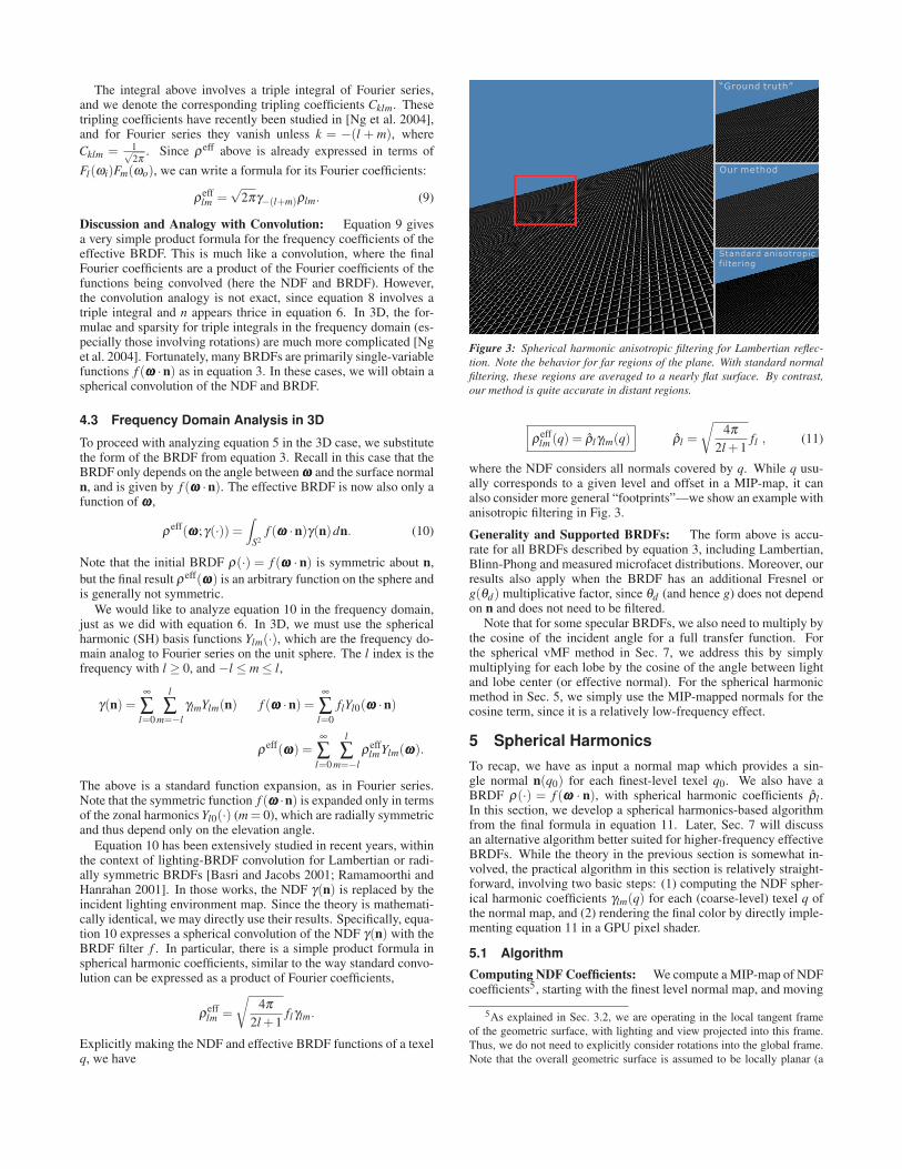
“Ground truth”

Figure 3: Spherical harmonic anisotropic filtering for Lambertian reflec-

tion. Note the behavior for far regions of the plane. With standard normal

filtering, these regions are averaged to a nearly flat surface. By contrast,

our method is quite accurate in distant regions.

ρefflm (q) = ρ̂lγlm(q) ρ̂l =

√

4π

2l +1fl , (11)

where the NDF considers all normals covered by q. While q usu-ally corresponds to a given level and offset in a MIP-map, it canalso consider more general “footprints”—we show an example withanisotropic filtering in Fig. 3.

Generality and Supported BRDFs: The form above is accu-rate for all BRDFs described by equation 3, including Lambertian,Blinn-Phong and measured microfacet distributions. Moreover, ourresults also apply when the BRDF has an additional Fresnel org(θd) multiplicative factor, since θd (and hence g) does not dependon n and does not need to be filtered.

Note that for some specular BRDFs, we also need to multiply bythe cosine of the incident angle for a full transfer function. Forthe spherical vMF method in Sec. 7, we address this by simplymultiplying for each lobe by the cosine of the angle between lightand lobe center (or effective normal). For the spherical harmonicmethod in Sec. 5, we simply use the MIP-mapped normals for thecosine term, since it is a relatively low-frequency effect.

5 Spherical Harmonics

To recap, we have as input a normal map which provides a sin-gle normal n(q0) for each finest-level texel q0. We also have aBRDF ρ(·) = f (ωωω · n), with spherical harmonic coefficients ρ̂l .In this section, we develop a spherical harmonics-based algorithmfrom the final formula in equation 11. Later, Sec. 7 will discussan alternative algorithm better suited for higher-frequency effectiveBRDFs. While the theory in the previous section is somewhat in-volved, the practical algorithm in this section is relatively straight-forward, involving two basic steps: (1) computing the NDF spher-ical harmonic coefficients γlm(q) for each (coarse-level) texel q ofthe normal map, and (2) rendering the final color by directly imple-menting equation 11 in a GPU pixel shader.

5.1 Algorithm

Computing NDF Coefficients: We compute a MIP-map of NDFcoefficients5, starting with the finest level normal map, and moving

5As explained in Sec. 3.2, we are operating in the local tangent frame

of the geometric surface, with lighting and view projected into this frame.

Thus, we do not need to explicitly consider rotations into the global frame.

Note that the overall geometric surface is assumed to be locally planar (a

to coarser levels. At the finest level (denoted by subscript 0), γ(q0)is a delta distribution at n(q0), i.e., γ(q0) = δ (n−n(q0)) with cor-

responding spherical harmonic coefficients6

γlm(q0) = Ylm(n(q0)).

An important insight is that, unlike the original normals, thesespherical harmonic NDF coefficients γlm(q0) can now correctly belinearly filtered or averaged for coarser levels γlm(q). Hence, wecan simply MIP-map the spherical harmonic coefficients γlm(q0) inthe standard way, and no non-linear fitting is required.

Rendering: Rendering requires knowing the NDF coefficientsγlm(q), the BRDF coefficients ρ̂l , and then applying equation 11.We have already computed a MIP-map of NDF coefficients. Atthe time of rendering, we also know the BRDF. For many analyticmodels, formulae for ρ̂l are known [Ramamoorthi and Hanrahan

2001]. For example, for Blinn-Phong, ρ̂l ∼ e−l2/2s where s is thePhong exponent. For measured reflectance, ρ̂l is obtained directlyby a spherical harmonic transform of f (ωωω ·n).

Now, we can compute the spherical harmonic coefficients of theeffective BRDF, per equation 11. Finally, to evaluate it, we mustexpand in terms of spherical harmonics,

ρeff(ωωω,q) =l∗

∑l=0

l

∑m=−l

ρ̂lγlm(q)Ylm(ωωω), (12)

where ωωω(ωωω i,ωωωo) depends on the BRDF as usual (such as incidentdirection ωωω = ωωω i for Lambertian or halfway-vector ωωω = ωωωh forspecular), and l∗ is the maximum l used in the shader (accurate

results generally require l∗ ∼√

4s where s is the Blinn-Phong ex-ponent). For shading, assume a single point light source for now.At each surface location, we know the incident and outgoing direc-tions, so it is easy to find the half-vector ωωωh or other parameteriza-tion ωωω , and then use the BRDF formula above for rendering.7

We implement equation 12 in a pixel shader using GLSL (see ourwebsite for example code). The spherical harmonics Ylm are storedin floating point textures, as are the MIP-mapped NDF coefficientsγlm(q). Real-time frame rates are achieved comfortably for up to 64spherical harmonic terms (l∗ ≤ 7, corresponding to a Blinn-Phongexponent s≤ 12 or a Torrance-Sparrow surface roughness σ ≥ 0.2).

5.2 Results

Lambertian Reflection: In the Lambertian case, using only ninespherical harmonic coefficients (l ≤ 2) suffices [Ramamoorthi andHanrahan 2001]. An example is shown in Fig. 3. This figure alsoshows the generality of our method in terms of the footprint fortexel q, by using GPU-based anisotropic filtering, instead of MIP-mapping. Note that we preserve accuracy in far away regions of theplane, while naïve averaging of the normal produces a nearly flatsurface that is much darker than the actual (as illustrated in Fig. 1e).

Low-Frequency Specularities and Measured Reflectance:Specular materials with BRDF f (ωωωh ·n) also fit within our frame-work. The BRDF can also be changed at run-time, since the NDFis independent of it. We have factored all of the materials in thedatabase of [Matusik et al. 2003], using the f (θh)g(θd) factoriza-tion in [Lawrence et al. 2006]. Figure 4 shows two examples ofdifferent materials, which we can switch between at runtime.

Figure 5 shows closeup views from an animation sequence ofcloth draping over a sphere, using the blue fabric material from the

single “geometric normal”) over the region being filtered.6We use the real form of the spherical harmonics, rather than the com-

plex form, to simplify implementation. Otherwise, γlm(q0) = Y ∗lm(n(q0)).7Our spherical harmonic algorithm does not explicitly address color tex-

tures; a simple approximation would be to MIP-map them separately, and

then modulate the scalar result in equation 12. A more correct approach to

filtering material properties is discussed for our vMF method in Sec. 7.3.

“Leather” “Violet Rubber”

Figure 4: Our spherical harmonic algorithm for normal mapping, with two

of the materials in the Matusik database—we can support general measured

BRDFs and change reflectance or material in real time. Notice also the

correct filtering of the zoomed out view, shown at the bottom right.

Matusik database. Note the accuracy of our method (compare (b)with the supersampled “ground truth” in (c)). Also note the smoothtransition between close (unfiltered) and distant (fully filtered) re-gions in (a) and (b), as well as the filtered zoomed out view in (d).

Discussion and Limitations: Our spherical harmonic methodis a practical approach for low-frequency materials. Unlike pre-vious techniques, all operations are linear—no nonlinear fitting isrequired, and we can handle arbitrary lobe shapes and functionsf (ωωωh · n). Moreover, the BRDF is decoupled from the NDF, en-abling simultaneous changes of BRDF, lighting and viewpoint.

As with all low-frequency approaches, our spherical harmonicmethod requires many terms for high-frequency specularities (aBlinn-Phong exponent of s = 50 needs about 200 coefficients). Thefollowing sections provide more practical solutions in these cases.

6 Spherically Symmetric Distributions

Spherical harmonics are a suitable basis for representing low-frequency functions, but are impractical for higher-frequency func-tions due to the large number of coefficients required. For higher-frequency NDFs, then, we will instead use radially symmetric ba-sis functions, which are one-dimensional and therefore much morecompactly represented. By performing an offline optimization, weapproximate the NDF at each texel as the sum of a small number ofsuch lobes. Our approach is inspired by the symmetric Phong lobesused in [Fournier 1992], and effectively formalizes that methodwithin our convolution framework.

6.1 Basic Theoretical Framework for using SRBFs

Consider a single basis function γ(n · µµµ) for the NDF, symmetricabout some central direction µµµ . For now, γ is a general sphericalradial basis function (SRBF). Equation 10 now becomes

ρeff(ωωω ·µµµ;γ(·)) =∫

S2f (ωωω ·n)γ(n ·µµµ)dn.

It can be shown (for example, see [Tsai and Shih 2006]) that ρeff

is itself radially symmetric about µµµ (hence the form ρeff(ωωω · µµµ)above), and its spherical harmonic coefficients are given by

ρeffl = ρ̂lγl . (13)

Compared to equation 11, this is a simpler 1D convolution, sinceall functions are radially symmetric and therefore one-dimensional.To represent general functions, we can use a small number of repre-sentative lobes γl, j . Note that the calculation of the lobe directions

(a) Our method, f rame 1 (b) Our method, f rame 2 (c) “Ground truth”, f rame 2 (d) Our method, zoomed out

Figure 5: Stills from a sequence of cloth draping over a sphere, with closeups indicating correct normal filtering using our spherical harmonic algorithm (the

full movie is shown in the video). Note the smooth transition from the center (almost no filtering) to the corners (fully filtered) in (b)—compare also with ground

truth in (c). (d) is a zoomed out view that also filters correctly. We use a blue fabric material from the Matusik database as the BRDF.

is generally a nonlinear process; our particular implementation isgiven in Sec. 7.

For rendering, we need to expand the effective BRDF in spheri-cal harmonics, analogously to equation 12, but now using only them = 0 terms. Considering the summation of J lobes, we obtain

ρeff(ωωω,q) =J

∑j=1

∞

∑l=0

ρ̂lγl, j(q)Yl0(ωωω ·µµµ j), (14)

where we again make clear that the NDF γl, j is a function of thetexel q. This equation can be used directly for shading once we findωωω for the light source and view direction.

6.2 Discussion: Unifying Framework and Multiscale

Our theoretical framework in Sec. 6.1 unifies many normal filteringalgorithms. Previous lobe- or peak-fitting methods can be seen asspecial cases. For instance, [Schilling 1997; Toksvig 2005] effec-tively use a single lobe (J = 1), while [Fournier 1992] uses multiplePhong lobes for γ(n · µµµ). These methods have generally adoptedsimple heuristics in terms of the BRDF. By developing a generalconvolution framework, we show how to separate the NDF from theBRDF. Since we properly account for general BRDFs ρ̂l , we caneven change BRDFs on the fly—in contrast, even [Tan et al. 2005]is limited to predetermined Gaussian Torrance-Sparrow BRDFs.

Equation 13 has an interesting multi-scale interpretation, as de-picted in Fig. 6. At the finest scale (a), the geometry used is theoriginal highest-resolution normal map. Therefore, the NDF is adelta distribution at each texel, and the effective BRDF ρeff

l = ρ̂l .At coarser scales, the shading geometry used is effectively a fil-tered version of the fine-scale normal map, with the NDF becomingsmoother from (b)-(d). The effective BRDF is now filtered by thesmoothed NDF, essentially representing the complex fine-scale ge-ometry as a blurring of the BRDF.

Also note the symmetry between the BRDF and NDF in equa-tion 13. While the common fine-scale interpretation is for a deltafunction NDF and the original BRDF, we can also view it as a deltafunction BRDF and an NDF given by ρ̂l . These interpretations areconsistent with most microfacet BRDF models, which start by as-suming a mirror-like BRDF (delta function) and complex NDF (mi-crofacet distribution), and derive a net glossy BRDF on a smoothmacrosurface (delta function NDF).

6.3 Choice of Radial Basis Function

We now briefly discuss some possible approaches for approximat-ing and representing our radial basis functions γ(n · µµµ). One pos-sible method is to use zonal harmonics [Sloan et al. 2005]; how-ever, our high-frequency NDFs lead to large orders l, making fit-ting difficult and storage inefficient. An alternative is to use Gaus-sian RBFs, with parameters chosen using expectation maximization(EM) [Dempster et al. 1977]. In this case, we simply need to store3 parameters per SRBF: the amplitude, width and central direction.Whereas [Tan et al. 2005] pursued this approach using Euclidean

Figure 6: Illustration of multiscale filtering of the BRDF (rendered sphere)

and NDF (inset). (a) shows a closeup of the sphere, where we see the in-

dividual facets and a sharp NDF/effective BRDF. In (b), we have zoomed

out to where the geometry now appears smoother, although roughness is

still clearly visible. The effective BRDF is now blurred, now incorporating

finer-scale geometry. As we zoom further out in (c) and (d), the geometry

appears even smoother, while the BRDF is further filtered.

or planar (and therefore distorted) RBFs, we consider NDFs repre-sented on their natural spherical domain, which also enables us toderive a simple convolution formula.

Indeed, spherical Gaussian RBFs, such as in [Tsai and Shih2006] or Phong lobes, as in [Fournier 1992], are most appropri-ate. However, the nonlinear minimization required for fitting thesemodels is inefficient, given that we need to do so at each texel. In-stead, we use a spherical variant [Banerjee et al. 2005] of EM, withthe von Mises-Fisher8 (vMF) distribution [Fisher 1953]. Spheri-cal EM and vMFs have previously been used in other areas suchas computer vision [Hara et al. 2005] for approximating Torrance-Sparrow BRDFs; here we introduce them for the first time in com-puter graphics, to represent NDFs.

7 Spherical vMF Algorithm

We now describe our algorithms for fitting the NDF, and renderingwith mixtures of vMF lobes. The fitting is done using a technique

8For the unit 3D sphere, this function is also known as the Fisher dis-

tribution. We use the more general term von Mises-Fisher distribution, that

applies to n-dimensional hyperspheres.

known as spherical expectation maximization (EM) [Banerjee et al.2005]. EM is a common algorithm for fitting in statistics, that finds“maximum likelihood” estimates of parameters [Dempster et al.1977]. It is an iterative method, with each iteration consisting oftwo steps known as the E-step and the M-step. We use EM as op-posed to other fitting and minimization techniques because of itssimplicity, efficiency, robustness, and ability to work with sparsedata (the discrete normals in the NDF). We also show how to ex-tend the basic spherical EM algorithm to handle color and differentmaterials, create coherent lobes for hardware interpolation, and im-plement spherical harmonic convolution for rendering. Note thatwhile the theoretical development of this section is somewhat com-plicated, the actual implementation is quite simple, and full pseu-docode is provided in Algorithms 1 and 2.

7.1 Fitting NDF with Mixtures of vMFs

vMF distributions were introduced in statistics to model Gaussian-like distributions on the unit sphere (or hypersphere). An advantageof vMFs is that they are well suited to a spherical expectation max-imization algorithm to estimate their parameters. They are charac-terized by two parameters θ = {κ,µµµ} corresponding to the inversewidth κ and central direction µµµ . vMFs are normalized to integrateto 1, as required by a probability distribution, and are given by

γ(n ·µµµ ;θ) =κ

4π sinh(κ)eκ(n·µµµ). (15)

A mixture of vMFs (movMF) is defined as an affine combinationof vMF lobes θ j, with amplitude α j, where ∑ j α j = 1,

γ(n;Θ) =J

∑j=1

α jγ j(n ·µµµ j;θ j).

Here, θ j = {κ j,µ j} characterizes a single vMF lobe, and Θ stores

the parameters {α j,θ j}Jj=1 of all J vMFs in the movMF.

We use spherical EM (Algorithm 1) to fit a movMF to the nor-mals covered at each texel in the MIP-map. Line 5 of Algorithm 1shows the E-step. For all normals ni in a given texel, we computethe expected likelihood 〈zi j〉 that ni corresponds to lobe j. Lines 9-14 execute the M-step, which computes maximum likelihood esti-mates of the parameters. In practice, we seldom need more than10 iterations, so the full EM algorithm for a 512×512 normal mapconverges in under 2 minutes. Note that this is an offline computa-tion that needs to be done only once per normal map—unlike mostprevious work, it is also independent of the BRDF (and lighting).

Note the use of auxiliary variable r j in line 11, which represents〈x j〉/α j, where 〈x j〉 is the expected value of a random vector gener-ated according to the scaled vMF distribution γ(x;θ j). The centralnormal µµµ j and the inverse width κ j are related to r j by

r = A(κ)µµµ,

where A(κ) = coth(κ)− 1

κ. (16)

The direction µµµ is found simply by normalizing r (line 13), whileκ is given by A−1(‖r‖); since no closed-form expression exists for

A−1, we use the approximation in [Banerjee et al. 2005] (line 12).

Since EM is an iterative method, good initialization is important.For normal map filtering, we can proceed from the finest texels tocoarser levels. At the finest level, we have only a single normal ateach texel, so we need only a single lobe and directly set α = 1,µµµ = n, and κ to a large initial value. At coarser levels, a goodinitialization is to choose the furthest-apart J lobes from among the4J µµµ’s in the four finer-level texels; for this we use Hochbaum-Shmoys clustering [Hochbaum and Shmoys 1985]. Note that theactual fitting uses all normals covered by a given texel in the MIP-map.

Algorithm 1 The Spherical EM algorithm. Inputs are normals ni ina texel. Outputs are movMF parameters α , κ and µ for each lobe j.

1: repeat2: {The E-step}3: for all samples ni do4: for j = 1 to J do

5: 〈zi j〉 ← γ j(ni;θ j)

∑Jk=1 γk(ni;θk)

{Expected likelihood of ni in lobe j}

6: end for7: end for8: {The M-step}9: for j = 1 to J do

10: α j← ∑Ni=1〈zi j〉

N

11: r j← ∑Ni=1〈zi j〉ni

∑Ni=1〈zi j〉

{Auxiliary variable for κ,µµµ in equation 16}

12: κ j ← 3‖r j‖−‖r j‖31−‖r j‖2

13: µµµ j ← normalize(r j)14: end for15: until convergence

The accuracy of our method is shown in Fig. 7, where we see thatabout four lobes suffices in most cases, with excellent agreementwith six lobes. We also compare with the Gaussian EM fits of [Tanet al. 2005]. They work on a projection of the hemisphere onto theplane, and use standard Euclidean (rather than spherical) EM. Be-cause this planar projection introduces distortions, they have a sig-nificant loss of accuracy near the boundaries (top row). Our method(middle row) works on the natural spherical domain (hence the sideview shown), and is able to fit undistorted lobes anywhere on thesphere. Also note that [Tan et al. 2005] do not have an explicitconvolution formula, while our method can be combined with anyBRDF to produce accurate renderings (bottom row).

7.2 Spherical Harmonic Coefficients for Rendering

For rendering, we will need the spherical harmonic coefficients γl ofa normalized vMF lobe. To the best of our knowledge, these coeffi-cients are not found in the literature, so we derive them here basedon reasonable approximations. First, for large κ , we can assumethat sinh(κ) ≈ eκ/2. In practice, this approximation is accurate aslong as κ > 2, which is almost always the case. Hence, the vMF inequation 15 becomes

γ(n ·µµµ;θ)≈ κ

2πe−κ(1−n·µµµ).

Let β be the angle between n and µµµ . Then, 1−n ·µµµ = 1−cosβ .For moderate κ , β must be small for the exponential to be nonzero.In these cases, 1− cosβ ≈ β 2/2, and we get a Gaussian form,

γ(n ·µµµ ;θ)≈ κ

2πe−

κ2

β 2

. (17)

In [Ramamoorthi and Hanrahan 2001], the spherical harmoniccoefficients of a Torrance-Sparrow model of a similar form are com-

puted. For notational simplicity, let Λl =√

4π2l+1 . Then,

γ =e−β 2/(4σ 2)

4πσ2⇒ Λlγl = e−(σ l)2

. (18)

Comparing with equation 17, we obtain σ2 = 12κ and

Λlγl = e−σ 2l2

= e−l2

2κ . (19)

This formula provides us the desired spherical harmonic coeffi-cients γl for a vMF lobe, in terms of the inverse width κ .

Having obtained γl , we are now ready to proceed to rendering.Since each vMF lobe is treated independently, and the constants α j

and BRDF coefficients can be multiplied separately, we focus on

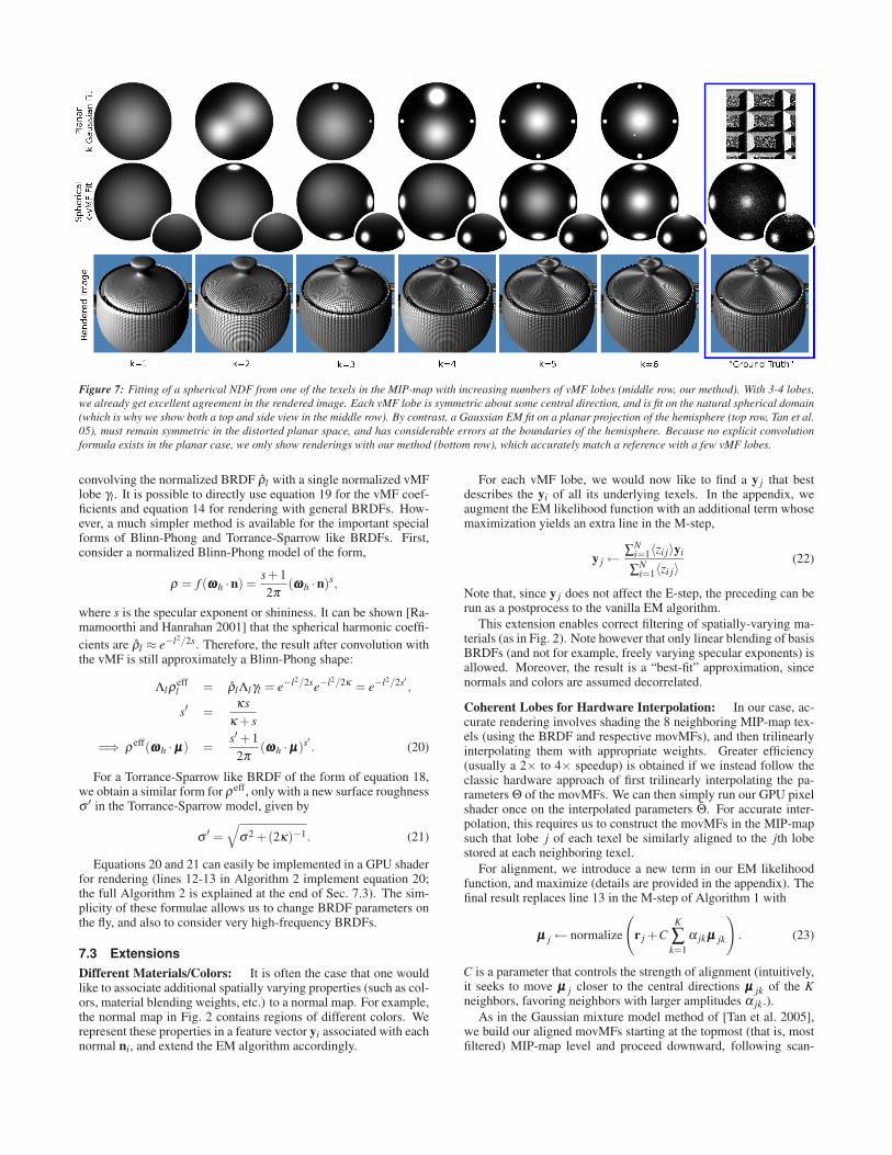
Figure 7: Fitting of a spherical NDF from one of the texels in the MIP-map with increasing numbers of vMF lobes (middle row, our method). With 3-4 lobes,

we already get excellent agreement in the rendered image. Each vMF lobe is symmetric about some central direction, and is fit on the natural spherical domain

(which is why we show both a top and side view in the middle row). By contrast, a Gaussian EM fit on a planar projection of the hemisphere (top row, Tan et al.

05), must remain symmetric in the distorted planar space, and has considerable errors at the boundaries of the hemisphere. Because no explicit convolution

formula exists in the planar case, we only show renderings with our method (bottom row), which accurately match a reference with a few vMF lobes.

convolving the normalized BRDF ρ̂l with a single normalized vMFlobe γl . It is possible to directly use equation 19 for the vMF coef-ficients and equation 14 for rendering with general BRDFs. How-ever, a much simpler method is available for the important specialforms of Blinn-Phong and Torrance-Sparrow like BRDFs. First,consider a normalized Blinn-Phong model of the form,

ρ = f (ωωωh ·n) =s+1

2π(ωωωh ·n)s,

where s is the specular exponent or shininess. It can be shown [Ra-mamoorthi and Hanrahan 2001] that the spherical harmonic coeffi-

cients are ρ̂l ≈ e−l2/2s. Therefore, the result after convolution withthe vMF is still approximately a Blinn-Phong shape:

Λlρeffl = ρ̂lΛlγl = e−l2/2se−l2/2κ = e−l2/2s′ ,

s′ =κs

κ + s

=⇒ ρeff(ωωωh ·µµµ) =s′+1

2π(ωωωh ·µµµ)s′ . (20)

For a Torrance-Sparrow like BRDF of the form of equation 18,we obtain a similar form for ρeff, only with a new surface roughnessσ ′ in the Torrance-Sparrow model, given by

σ ′ =√

σ2 +(2κ)−1. (21)

Equations 20 and 21 can easily be implemented in a GPU shaderfor rendering (lines 12-13 in Algorithm 2 implement equation 20;the full Algorithm 2 is explained at the end of Sec. 7.3). The sim-plicity of these formulae allows us to change BRDF parameters onthe fly, and also to consider very high-frequency BRDFs.

7.3 Extensions

Different Materials/Colors: It is often the case that one wouldlike to associate additional spatially varying properties (such as col-ors, material blending weights, etc.) to a normal map. For example,the normal map in Fig. 2 contains regions of different colors. Werepresent these properties in a feature vector yi associated with eachnormal ni, and extend the EM algorithm accordingly.

For each vMF lobe, we would now like to find a y j that bestdescribes the yi of all its underlying texels. In the appendix, weaugment the EM likelihood function with an additional term whosemaximization yields an extra line in the M-step,

y j←∑N

i=1〈zi j〉yi

∑Ni=1〈zi j〉

(22)

Note that, since y j does not affect the E-step, the preceding can berun as a postprocess to the vanilla EM algorithm.

This extension enables correct filtering of spatially-varying ma-terials (as in Fig. 2). Note however that only linear blending of basisBRDFs (and not for example, freely varying specular exponents) isallowed. Moreover, the result is a “best-fit” approximation, sincenormals and colors are assumed decorrelated.

Coherent Lobes for Hardware Interpolation: In our case, ac-curate rendering involves shading the 8 neighboring MIP-map tex-els (using the BRDF and respective movMFs), and then trilinearlyinterpolating them with appropriate weights. Greater efficiency(usually a 2× to 4× speedup) is obtained if we instead follow theclassic hardware approach of first trilinearly interpolating the pa-rameters Θ of the movMFs. We can then simply run our GPU pixelshader once on the interpolated parameters Θ̃. For accurate inter-polation, this requires us to construct the movMFs in the MIP-mapsuch that lobe j of each texel be similarly aligned to the jth lobestored at each neighboring texel.

For alignment, we introduce a new term in our EM likelihoodfunction, and maximize (details are provided in the appendix). Thefinal result replaces line 13 in the M-step of Algorithm 1 with

µµµ j← normalize

(

r j +CK

∑k=1

α jkµµµ jk

)

. (23)

C is a parameter that controls the strength of alignment (intuitively,it seeks to move µµµ j closer to the central directions µµµ jk of the Kneighbors, favoring neighbors with larger amplitudes α jk.).

As in the Gaussian mixture model method of [Tan et al. 2005],we build our aligned movMFs starting at the topmost (that is, mostfiltered) MIP-map level and proceed downward, following scan-

Algorithm 2 Pseudocode for the vMF GLSL fragment shader

1: {Setup: calculate half angle ωωωh and incident angle ωωω i}2: ρ ← 03: for j = 1 to J do {Add up contributions for all J lobes}4: {Look up vMF parameters stored in 2D texture map}5: θ ← texture2D(vMFTexture[ j],s, t)6: αy← texture2D(colorTexture[ j],s, t)7: α ← θ .x8: r← θ .yzw

α {θ .yzw stores αr}

9: κ ← 3‖r‖−‖r‖3

1−‖r‖2

10: µµµ ← normalize(r)11: {Calculate shading per equation 20}12: s′← κs

κ+s {s is Blinn-Phong exponent}

13: Bs← s′+12π (ωωωh ·µµµ)s′ {Equation 20}

14: ρ ← ρ +αy(KsBs +Kd)(ωωω i ·µµµ)15: end for16: gl_FragColor← L×ρ {L is light intensity}

line ordering within each individual level. In the interest of per-formance, we use only previously visited texels as neighbors.

We next consider trilinear interpolation of the variables. Unfor-tunately, the customary vMF parameters {κ,µµµ} control non-linearaspects of the vMF lobe and therefore cannot be linearly interpo-lated. To solve this problem, we recall from Sec. 7.1 that µµµ andκ can be inferred from the scaled Euclidean mean r = 〈x〉/α of agiven vMF distribution. By linearity of expectation, we can inter-polate αr = 〈x〉 linearly, as well as the amplitude α , giving

α̃ j = T (α j) r̃ j = T (α jr j)/T (α j),

where T (·) denotes trilinear hardware interpolation. Finally, κ̃ j andµ̃µµ j can easily be found in-shader (lines 9 and 10 of Algorithm 2).

Algorithm 2 shows pseudocode for our GLSL fragment shader.Lines 5-10 look up α and αr, and then compute κ and µ . For im-plementation, we store the jth lobe of each movMF in a standardRGBA MIP-map (vMFTexture in Algorithm 2) using one channelfor α and one channel each for the three components of αr. Nor-malized color/material properties αy are stored in correspondingtextures (colorTexture in line 6 of Algorithm 2). Line 5 reads theparameters θ for a single vMF lobe as an RGBA value. Lines 12-13compute the specular shading (assuming a Blinn-Phong model withexponent s) using equation 20. The Torrance-Sparrow model canbe handled similarly, using equation 21. Line 14 computes the finalshading contribution by including the color parameters y, and scal-ing by the lobe amplitude α , specular coefficient Ks, and the cosineof the incident angle, while adding the Lambertian component Kd .Note that this shader can be used equally with aligned or unalignedvMF lobes; the only difference is whether we manually computeand combine results from all 8 neighboring texels (unaligned) oruse hardware interpolate to first obtain lobe parameters (aligned).

7.4 Results

Figure 2 shows the accuracy of our method, and makes comparisonsto ground truth and alternative techniques. It also shows our abilityto use different materials for different parts of the normal map.

Our formulation allows for general and even dynamically chang-ing BRDFs. Figure 8 shows a complex scene, where the reflectancechanges over time, decreasing in shininess (intended to simulatedrying using the model in [Sun et al. 2007]). Although not shown,the lighting and view can also vary—the bottom row shows close-ups with different illumination. Note the correct filtering for di-nosaurs in the background, and for further regions along the neckand body of the foreground dinosaur. Even where individual bumpsare not visible, the overall change in appearance as the reflectancechanges is clear. This complex scene has 14,898 triangles for thedinosaurs, 139,392 triangles for the terrain and 6 different textures

Figure 8: Our framework can handle complex scenes, allowing for general

reflectance, which can even be changed at run-time. Here, the BRDF be-

comes less shiny over time. Note the correct filtering and overall changes in

appearance for further regions of the foreground dinosaur, and those in the

background. The bottom row shows closeups (when the material is shiny)

with a different lighting condition. This example also shows that we can

combine filtered normal maps with standard color texture mapping.

and normal maps for the dinosaur skins. It renders at 75 framesper second at a resolution of 640x480 on an nVIDIA 8800 graphicscard. In this example, we used six vMF lobes, with both diffuse andspecular shading implemented as a simple fragment shader. Pleasesee our website for videos of all of our examples.

8 Complex Lighting

Our vMF-based normal map filtering technique can also be ex-tended to complex environment map lighting.9 Equation 2,rephrased below, is a convolution (mathematically similar to equa-

9The direct spherical harmonic method in Sec. 5 is more difficult to ap-

ply, since general spherical harmonics cannot be rotated as easily as radially

symmetric functions between local and global frames.

Figure 9: Armadillo model with 350,000 polygons rendered interactively

with normal maps in dynamic environment lighting. We use 6 vMF lobes,

and spherical harmonics up to order 8 for the specular component.

tion 10), that becomes a simple dot product in spherical harmonics,

B(µµµ) =∫

S2L(ωωω i)ρ

eff(ωωω ·µµµ)dωωω i, (24)

where the effective BRDF ρeff is the convolution of the vMF lobewith the BRDF, and µµµ is the central direction of the vMF lobe(effective “normal”) as usual. For the diffuse or Lambertian com-ponent of the BRDF ωωω(ωωω i,ωωωo) = ωωω i, and the spherical harmoniccoefficients can simply be multiplied according to the convolutionformula, Blm = Λlρ

effl Llm, so that

B =l∗

∑l=0

l

∑m=−l

Λlρeffl LlmYlm(µµµ). (25)

However, the specular component of the BRDF is expressed interms of ωωω(ωωω i,ωωωo) = ωωωh, and we need to change the variable ofintegration in equation 24 to ωωωh (which leads to a factor 4(ωωω i ·ωωωh)),

B(µµµ) =∫

S2[L(ωωω i(ωωωh,ωωωo)) ·4(ωωω i ·ωωωh)]ρ

eff(ωωωh ·µµµ)dωωωh

=∫

S2L′(ωωωh)ρ

eff(ωωωh ·µµµ)dωωωh.

Thus, we simply need to consider a new reparameterized lightingL′(ωωωh) = L(ωωω i(ωωωh,ωωωo)) ·4(ωωω i ·ωωωh). As the half angle depends onboth viewing and lighting angles (ωωωo and ωωω i), the above integrationimplicitly limits us to a fixed view with respect to the lighting. Tointeractively rotate the lighting, we precompute a sparse set (typi-cally, about 16×16) of rotated lighting coefficients and interpolatethe shading.

Finally, in analogy with equation 25,

B =l∗

∑l=0

l

∑m=−l

Λlρeffl L′lmYlm(µµµ). (26)

Figure 9 shows an image of an armadillo, with approximately350,000 polygons and a normal map, rendered at real-time rates indynamic environment lighting. We are able to render interactivelywith up to 6 vMF lobes and l∗ = 8 in equation 26.

9 Conclusions and Future Work

We have developed a comprehensive theoretical framework for nor-mal map filtering with many common types of reflectance models.Our method is based on a new analytic formulation of normal mapfiltering as a convolution of the NDF and BRDF. This leads to novelpractical algorithms using spherical harmonics and spherical vMFs.The algorithms are simple enough to be implemented as GPU pixelshaders, enabling real-time rendering on graphics hardware.

We believe this paper also makes broader contributions to manyareas of rendering, and beyond. The convolution result unifies ageometric problem (normal mapping) with understanding of light-ing and BRDF interaction in appearance. Moreover, we introducespherical EM and vMF distributions into computer graphics, wherethey will likely find many other applications.

In [Kajiya 1985], a hierarchy of level-of-details was spelled outincluding explicit 3D geometry, normal or bump maps, and BRDFor reflectance. This paper has addressed filtering of normal mapsand to some extent, the transition to a BRDF at far distances. Acritical direction for future work is filtering of geometry or dis-placement maps, where effects like local occlusions, shadowing,masking and interreflections are important.

In summary, although normal mapping is an old technique, cor-rect filtering has been challenging because shading is nonlinear inthe surface normal. In this paper, we have shown how frequency-domain analysis reveals important new insights, and taken a signif-icant step towards addressing this long-standing problem.

Acknowledgements: We express our deep appreciation to theprimary referee for his detailed comments to improve the exposi-tion of this paper during “shepherding”. We are extremely gratefulto Tony Jebara for first pointing us towards vMF representations andspherical EM. Normal map filtering and multiscale representationsare a long-standing problem, and we have had many discussions(and initial efforts at a solution) with a number of researchers overthe years including Aner Ben-Artzi, Peter Belhumeur, Pat Hanra-han, Shree Nayar, Evgueni Parilov, Makiko Yasui and Denis Zorin.This work was funded in part by NSF grants #0305322, #0446916,#0430258, #0528402, #0614770, #0643268, a Sloan Research Fel-lowship, a Columbia University Presidential Fellowship, and anONR Young Investigator award N00014-07-1-0900. We also wishto thank NVIDIA for a generous donation of their latest graphicscards during the deadline crunch.

References

BANERJEE, A., DHILLON, I., GHOSH, J., AND SRA, S. 2005.Clustering on the unit hypersphere using von Mises-Fisher dis-tributions. Journal of Machine Learning Research 6, 1345–1382.

BASRI, R., AND JACOBS, D. 2001. Lambertian reflectance andlinear subspaces. In International Conference on Computer Vi-sion, 383–390.

BECKER, B., AND MAX, N. 1993. Smooth transitions betweenbump rendering algorithms. In SIGGRAPH 93, 183–190.

BLINN, J. 1978. Simulation of wrinkled surfaces. In SIGGRAPH78, 286–292.

CLAUSTRES, L., BARTHE, L., AND PAULIN, M. 2007. WaveletEncoding of BRDFs for Real-Time Rendering. In Graphics In-terface 07.

COHEN, J., OLANO, M., AND MANOCHA, D. 1998. Appearancepreserving simplification. In SIGGRAPH 98, 115–122.

DEMPSTER, A., LAIRD, N., AND RUBIN, D. 1977. Maximum-likelihood from incomplete data via the EM algorithm. Journalof the Royal Statistical Society, Series B 39, 1–38.

FISHER, R. 1953. Dispersion on a sphere. Proceedings of theRoyal Society of London, Series A 217, 295–305.

FOURNIER, A. 1992. Normal distribution functions and multiplesurfaces. In Graphics Interface Workshop on Local Illumination,45–52.

HARA, K., NISHINO, K., AND IKEUCHI, K. 2005. Multiple lightsources and reflectance property estimation based on a mixtureof spherical distributions. In ICCV ’05: Proceedings of the TenthIEEE International Conference on Computer Vision, 1627–1634.

HECKBERT, P. 1989. Fundamentals of texture mapping and imagewarping. Master’s thesis, UC Berkeley UCB/CSD 89/516.

HOCHBAUM, D., AND SHMOYS, D. 1985. A best possible heuris-tic for the k-center problem. Mathematics of Operations Re-search.

HORN, B. K. P. 1984. Extended gaussian images. Proceedings ofthe IEEE 72, 1671–1686.

KAJIYA, J. 1985. Anisotropic reflection models. In SIGGRAPH85, 15–21.

LALONDE, P., AND FOURNIER, A. 1997. A wavelet representationof reflectance functions. IEEE TVCG 3, 4, 329–336.

LAWRENCE, J., BENARTZI, A., DECORO, C., MATUSIK, W.,PFISTER, H., RAMAMOORTHI, R., AND RUSINKIEWICZ, S.2006. Inverse shade trees for non-parametric material represen-tation and editing. ACM Transactions on Graphics (SIGGRAPH2006) 25, 3, 735–745.

MATUSIK, W., PFISTER, H., BRAND, M., AND MCMILLAN, L.2003. A data-driven reflectance model. ACM Transactions onGraphics (SIGGRAPH 03 proceedings) 22, 3, 759–769.

NG, R., RAMAMOORTHI, R., AND HANRAHAN, P. 2004. Tripleproduct wavelet integrals for all-frequency relighting. ACMTransactions on Graphics (SIGGRAPH 2004) 23, 3, 475–485.

OLANO, M., AND NORTH, M. 1997. Nor-mal distribution mapping. Tech. Rep. 97-041http://www.cs.unc.edu/~olano/papers/ndm/ndm.pdf, UNC.

RAMAMOORTHI, R., AND HANRAHAN, P. 2001. A signal-processing framework for inverse rendering. In SIGGRAPH 01,117–128.

SCHILLING, A. 1997. Toward real-time photorealistic rendering:Challenges and solutions. In SIGGRAPH/Eurographics Work-shop on Graphics Hardware, 7–16.

SLOAN, P., KAUTZ, J., AND SNYDER, J. 2002. Precomputed radi-ance transfer for real-time rendering in dynamic, low-frequencylighting environments. ACM Transactions on Graphics (SIG-GRAPH 02 proceedings) 21, 3, 527–536.

SLOAN, P., LUNA, B., AND SNYDER, J. 2005. Local, deformableprecomputed radiance transfer. ACM Transactions on Graphics(SIGGRAPH 05 proceedings) 24, 3, 1216–1224.

STREHL, A., GHOSH, J., AND MOONEY, R. 2000. Impact ofsimilarity measures on web-page clustering. In Proc Natl Confon Artificial Intelligence : Workshop of AI for Web Search (AAAI2000), 58–64.

SUN, B., SUNKAVALLI, K., RAMAMOORTHI, R., BELHUMEUR,P., AND NAYAR, S. 2007. Time-Varying BRDFs. IEEE Trans-actions on Visualization and Computer Graphics 13, 3, 595–609.

TAN, P., LIN, S., QUAN, L., GUO, B., AND SHUM, H. 2005.Multiresolution reflectance filtering. In EuroGraphics Sympo-sium on Rendering 2005, 111–116.

TOKSVIG, M. 2005. Mipmapping normal maps. Journal of Graph-ics Tools 10, 3, 65–71.

TSAI, Y., AND SHIH, Z. 2006. All-frequency precomputed radi-ance transfer using spherical radial basis functions and clusteredtensor approximation. ACM Transactions on Graphics (SIG-GRAPH 2006) 25, 3, 967–976.

WILLIAMS, L. 1983. Pyramidal parametrics. In SIGGRAPH 83,1–11.

Appendix: Spherical EM Extensions

In this appendix, we briefly describe the likelihood function forspherical EM, and how we augment it for colors/materials and co-herent lobes. The net likelihood function is a product of 3 terms,

P(X ,Z|Θ)P(Y,Z|Θ)P(Θ|N(Θ)),

where X are the samples (in this case input normals), Y are the col-ors/materials, Z are the hidden variables (in this case which vMFlobe a sample X is drawn from), Θ are parameters for all vMF lobesand N(Θ) are parameters for neighbors. The first factor correspondsto standard spherical EM, the second factor corresponds to the col-ors/materials Y ,

P(Y,Z|Θ) =N

∏i=1

e−‖yzi−yi‖2

,

and the final factor to coherent lobes for interpolation,

P(N(Θ)|Θ) =J

∏j=1

K

∏k=1

eC′α jk(µµµ j ·µµµ jk).

We use C′ above as a constant weighting factor (it will be related tothe weight C used in the main text as discussed below).

In EM, we seek to maximize the log likelihood

ln [P(X ,Z|Θ)P(Y,Z|Θ)P(Θ|N(Θ))] =

N

∑i=1

lnγ(ni|θzi)+

N

∑i=1

−‖yi−yzi‖2 +

J

∑j=1

K

∑k=1

C′α jk(µµµ j ·µµµ jk) ,

which, considering all J lobes and hidden variables 〈zi j〉, becomes

J

∑j=1

[

N

∑i=1

lnγ(ni|θ j)〈zi j〉+N

∑i=1

−‖yi−yzi‖2〈zi j〉+

K

∑k=1

C′α jk(µµµ j ·µµµ jk)

]

.

Maximizing with respect to y j, we directly obtain equation 22. Themaximization with respect to µµµ j is more complex,

µµµ j = normalize

(

κ j

N

∑i=1

ni〈zi j〉+C′K

∑k=1

α jkµµµ jk

)

.

Finally, redefining C = C′/κ j , we obtain equation 23.