Free Trade as a Repeated Game

Mat-2.4108 Independent research project in applied mathematics

Helsinki University of Technology

System Analysis Laboratory

Lassi Ahlvik, 64439M

Espoo, 30.5.2009

Abstract

The most important economies in the world have agreed to open trade and reduce trade barriers

little by little since the end of the Second World War. Regardless of these agreements, every so

often countries decide to violate them by creating trade barriers. In this work we try to find out

whether these violations are made from economic basis. Our objective is to give a brief

introduction in the theory of free trade and trade wars using game theory, and measure

conditions in which free trade agreements are sustainable and beneficial for all participants.

Key words: free trade, trade war, optimal tariff, repeated prisoner’s dilemma

Contents

1. Introduction ........................................................................................................ 1

2. Basics of free trade .............................................................................................. 2

2.1 Theory of comparative advantage ..................................................................................... 2

2.2 More arguments for free trade ......................................................................................... 5

2.3 Arguments against free trade............................................................................................ 5

3. Game theoretical analysis ................................................................................... 6

3.1 The trade war ................................................................................................................... 6

3.2 Basic consepts of game theory .......................................................................................... 8

3.3 Nash equilibrium of a one-shot game................................................................................ 8

3.4 Nash equilibrium of a repeated game ............................................................................. 11

4. Example: The Transatlantic Free Trade Union .................................................. 15

5. Conclusion ......................................................................................................... 17

References ............................................................................................................... 18

1

1. Introduction

The global economy has gone a long way since the end of the Second World War. After the war

rivalry with the communist bloc forced capitalist countries to cooperate as contrary to the pre-war

isolationist and protectionist policies. This cooperation led to opening of trade by several

international agreements and eventually to founding of the World Trade Organization (WTO) in

1995. This international institution was designed to control and accelerate the liberalization of

trade globally. By the side of global lowering of tariffs, there is another, maybe even more

important ongoing process: bilateral free trade agreements.

The term free trade refers to a governmental policy of that allows trading to happen without

governmental intervention. In certain circumstances countries choose to violate either bilateral or

WTO agreement and start a trade war with another participant. In a trade war a country imposes a

trade barrier which is retaliated by other countries’ trade barriers. Government has various tools

to restrict trade. The most used one throughout history has been tariff, an import or export tax. A

trade quota means a limit for the amount of goods that can be imported or exported in a certain

amount of time. Subsidies are paid from the governmental budget to support certain domestic

industries. Means that are not directly related to trade, such as high quality standards, are

becoming more popular because they are harder to police by WTO.

There is a consensus between economists that free trade is beneficial for the world as a whole,

and a trade war always has a negative impact on the overall welfare. However, the pareto

optimality of free trade is still under discussion. In the theory of international trade it is usually

assumed that the countries are small and their trade volumes are not big enough to affect world

prices [6][13]. This holds true for some of the commodities, but in many industries a single country

can be a significant actor, and their actions affect on other outcomes of other countries hence

making the problem game theoretical.

Traditionally economists have used a 2x2-model (two countries, two goods) to examine effects of

free trade in a game theoretical context. De Scitovszky (1942) points out that a tariff increases the

welfare of a country temporarily, but it leads to retaliatory measures by the other side thus

leaving both countries worse off [4]. Johnson (1953-1954) proved this conclusion wrong ten years

2

later. According to him, a country can win a tariff war despite retaliation, if its elasticity of demand

for imports is significantly higher than opponent’s [9]. Kennan, Riezman (1988) and Syropoulos

(2002) continued the research of Johnson by studying the impact of relative sizes of countries on

the outcome of tariff wars [10][16]. Both researches agree that a significantly bigger country can

win a tariff war and therefore free trade does not occur between countries of different sizes.

Kreinin, Dinopoulos and Constantinos (1996) examined a bilateral trade war with three countries:

an exporter, an importer and a freely trading country [11]. They found out that it is also possible to

win a trade war despite of the presence of a neutral country. Naya and Naya (2007) studied tariff

wars in imperfectly competitive markets [14]. They claim that free trade is not sustainable for

countries of unequal sizes, and even for equally big countries free trade is not strictly preferable

option.

Primary goal of this research project is to give a brief overview on the topic of free trade by

introducing economic and non-economic arguments for and against free trade. We use the theory

of comparative advantage to prove that an unrestricted trade is the most efficient option for the

entire world. After that we will take a look on how free trade affects on single countries by taking

a look on the mathematics behind free trade agreements between two big countries. We will find

conditions under which a sustainable free trade is possibly by following the approach of Kennan

and Riezman. Another goal of this research is to improve the work of Kennan and Riezman. They

found conditions under which big countries win trade wars in the long run [10], but we make the

model more detailed by including also short-term profits for countries.

2. Basics of free trade

2.1 Theory of comparative advantage

The most principal argument for efficiency of free trade is a theory of comparative advantage

introduced by David Ricardo in 1817. It is a simple mathematical model that predicts an intuitive

result: the utility level of the world is higher if countries trade freely. The concept of comparative

advantage is not always easily believed by free-trade skeptics, and that is why Krugman even

3

called it “an idea that conflicts with both stubborn popular and powerful interests” [12]. This

model was later on completed by Heckscher and Ohlin [6].

The basic assumption of the theory is that different goods require different factors to produce,

and countries differ in their factor endowments. If a country uses fewer resources to produce a

certain good than another country, the country has an absolute advantage in that good over the

competitor. The country is said to have a comparative advantage over another country if it loses

less alternative production opportunities in producing certain good. For example Russia has a

small absolute advantage over Finland in labor-abundant products such as clothes, and a huge one

in land-abundant products such as wood because of its land and labor resources. Even so Finland

has a comparative advantage in labor-abundant clothes because producing clothes is cheaper in

terms of lost wood.

For simplicity we assume a two-country model in which both countries produce only two products.

Country 1 has an absolute advantage in both goods and a comparative advantage in good A, and

country 2 has a comparative advantage in good B. The production possibilities are drawn in Figure

1, in which 𝑎𝑖 and 𝑏𝑖 mean the maximum amounts of goods A and B country i can produce. From

absolute and comparative advantages, we get the following inequalities:

𝑎1 > 𝑎2 , 𝑏1 > 𝑏2, 𝑎1

𝑏1>

𝑎2

𝑏2 . (1)

The production possibility function (PPF) for each country is a line on where all the limited

resources are efficiently used, and increase in production of one good cannot be done without a

reduction in production of another good. For country 1 𝑃𝑃𝐹1is the line between plots 𝑎1 and 𝑏1,

and for country 2 𝑃𝑃𝐹2 is the line between 𝑎2 and 𝑏2 in Figure 1.

We can draw an indifference curve which shows all possible alternatives for goods between which

consumers are indifferent. The standard assumptions for indifference curves are downward

sloping and convex [6]. The utility of consumers increases when the indifference curve moves

right, because it increases the number of consumption opportunities. The optimal consumption

choice is the location where indifference curve touches the PPF –line, because in that point utility

cannot be increased without changing production possibilities. 𝐼𝑖 represents an indifference curve

for the country i, and P and Q are points where utility is maximized.

4

Figure 1: Consumption alternatives under restricted trade and optimal solutions

If there are no restrictions for trade countries can specialize on goods they have the comparative

advantage in and trade the extra production with the other country. In Figure 2 we get 𝑃𝑃𝐹𝑊 for

the whole world by adding up the two individual PPF’s. As we see, this frontier is kinked, and the

corner point is point in which both countries are fully specialized in one product. We can see that

the optimal point on 𝑃𝑃𝐹𝑊 is on higher utility level than the point P+Q which represents

combined utility of two producing countries. This proves that the most efficient outcome is gotten

when countries specialize in products with comparative advantage.

Figure 2: Consumption alternatives under free trade

5

2.2 More arguments for free trade

Besides of theory of comparative advantage, there are also numerous non-economic arguments

for free trade. Antweiler et al. studied the impact of free trade on quality of the environment by

observing sulfur dioxide levels in different countries over time [1]. Free trade affects on the

environments of opening countries in three ways. The first one is the technique effect which

means the opportunity to buy more environmental friendly producing technologies by the

increased income from free trade. According to that the free trade has a positive effect on the

environment. The second one, scale effect, has a negative effect on the environment because of

increased volume in production. The third one is so called composition effect which alters the

production patterns of the country towards industries in which country has a comparative

advantage. Effect has either positive or negative consequences on the environment depending on

factor endowments of the country. Pollution haven hypothesis predicts that poor countries have

advantage in polluting industries because their pollution policies are less strict and that is why

poor countries get dirtier and rich countries cleaner when the trade opens up. According to the

authors, the technique effect dominates and freer trade seems to be good for the environment. As

Irwin summarizes: “environmental damage results from poor environmental policies, not poor

trade policies” [8].

Many economists and political scientists have the idea that trade promotes peace. The idea is that

the economic interdependence raises the cost of war makes waging a war less profitable. Some

economists disagree with this: although there is a proven correlation between openness of trade

and war, it is unclear what the cause is and what is the effect, because less aggressive countries

are more willing to adopt free trade policies [8].

2.3 Arguments against free trade

Like pro free trade arguments, also arguments against free trade can be split it two categories:

economic and non-economic. Although the theory of comparative advantage undeniably proves

that unrestricted trade is the most efficient solution in world scale, it is not necessarily optimal for

each participant. As Syropoulos, Kennan and Riezman pointed out, big countries can imply a tariff

6

and be better off even after the retaliatory actions [16][10]. As we point out later on, also high

interest rate levels and political instabilities make free trade less preferable option.

Another argument for protectionism is an infant industry argument: a small domestic industry

cannot compete with foreign firms, and therefore government has to impose tariffs to protect the

industry until it becomes strong enough to thrive globally. Some economists such as Baldwin and

Gandolfo however disagree with the argument claiming that infant tariffs may decrease the social

welfare especially in the short run [3][6].

The most common non economic arguments according to Gandolfo are national security, foreign

policy and national pride [6]. An example of the first one is an arms trade: countries do not want

to arm possibly hostile nations even if it would be economically efficient. The foreign policy

argument is used when countries use economic means to achieve political goals, for instance of

trade embargoes. The national pride argument claims that producing certain commodity can build

up nationalism just like winning medals in Olympics.

3. Game theoretical analysis

3.1 The trade war

The trade war is considered to be a game between two countries with following assumptions:

1) Countries trade only with each other

2) Countries produce and consume only two goods

3) The only way to restrict trade is an import tariff

4) Countries are identical, except for differences in endowments

5) Countries aim to maximize their increasing utility functions

6) Perfect information exists.

As assumed before in chapter 2.1., in a world with no tariffs country 1 would be net exporter of

good A and net importer of good B because of comparative advantage mentioned in the previous

chapter. Respectively country 2 would to be net importer of good A and net exporter of good B.

Country 1 possesses portion 𝛾 of good A and (1 − 𝜇) of good B, and country B owns the rest.

7

In order to form the game in strategic form we have to find out utilities for both countries in

respect of their choice of tariff. However measuring utility is not unambiguous, but depends on

the preferences of decision making agents. In this work the decision making body of both

countries are assumed to be democratically elected parliaments which represent the people and

aim to maximize the utility of citizens. Later on, whenever we talk about countries maximizing

their utility, we actually mean governments maximizing the utility of the citizens. For simplicity we

assume that the utility function for people of country i has the form

𝑈𝑖 = 𝐴𝑖𝐵𝑖 , (2)

where 𝐴𝑖 and 𝐵𝑖 are the amounts of goods available for that country. The governments can

interfere by adding a tariff 𝑡𝑖 = 𝑆𝑖 − 1 on its imports which lifts the price of imports to 𝑆1𝑃𝐵 for

country 1 and 𝑆2𝑃𝐴 if 𝑃𝐴 and 𝑃𝐵 are the prices of goods. The maximization problem has a budget

constraint that consists of goods the country already owns, and the tariff revenue.

𝑃𝐴𝐴1 + 𝑆1𝑃𝐵𝐵

1 = 𝑃𝐴𝛾 + 𝑆1𝑃𝐵 1 − 𝜇 + (𝑆1 − 1)𝑃𝐵𝐵 (3)

for country 1. In future we examine this problem from the viewpoint of country 1, and analogous

results for country 2 are not written down. To maximize the utility in (2) we have to use the same

amount of money on both goods

𝑃𝐴𝐴1 = 𝑆1𝑃𝐵𝐵

1. (4)

The affordable amount of good A left for country 1 is the original amount minus exports, and for

good B it is the sum of original amount and imports. 𝐴 and 𝐵 refer to amounts of exported goods.

Using (4) this can be written as

𝑃𝐴(𝛾 − 𝐴) = 𝑆1𝑃𝐵(1 − 𝜇 + 𝐵). (5)

By combining (3) and (5) we get the connection between amount of exports, imports and

possessed resources as follows

𝛾 = 𝑆1(1−𝜇 )

𝐵+ 𝑆1 + 1 𝐴 (6)

We assume both countries behave rationally and try to maximize their utility function (2), which

can be written as

8

𝑈1 = (𝛾 − 𝐴)(1 − 𝜇 + 𝐵). (7)

By using the equation (6) and the similar equation for country 2 we can eliminate A and B and

form the utility function for country 1

𝑈1(𝑆1 ,𝑆2) =[𝛾+ 1−𝜇 𝑆2]2

1+ 1−𝜇 𝑆2+𝜇

𝑆1 [𝑆2 + 1−𝛾 𝑆1𝑆2+𝛾]

. (8)

3.2 Basic consepts of game theory

In game theory players, called agents, have a variety of actions, called strategies, to choose from

in a certain game. A game in strategic form consists of a set of agents and set of strategies for each

agent. Each agent’s utility is depended not just the strategy 𝑠𝑖 he chooses from his set, but also

strategies chosen by other agents in the game 𝑢𝑖 = 𝑢𝑖(𝑠1,…𝑠𝑛).

The definition of Nash equilibrium is following: In the n-player normal-form game 𝐺 =

{𝑆1 ,… ,𝑆𝑛 ; 𝑢1,… , 𝑢𝑛 }, the strategies (𝑠1∗,… , 𝑠𝑛

∗) are a Nash equilibrium if, for each player i, 𝑠𝑖∗ is (at

least tied for) player i’s best response ti the strategies specified for the n-1 other players,

(𝑠1∗,…𝑠𝑖−1

∗ , 𝑠𝑖+1∗ ,… , 𝑠𝑛

∗):

𝑢𝑖(𝑠1∗,…𝑠𝑖−1

∗ , 𝑠𝑖∗ , 𝑠𝑖+1

∗ ,… , 𝑠𝑛∗) ≥ 𝑢𝑖(𝑠1

∗ ,…𝑠𝑖−1∗ , 𝑠𝑖 , 𝑠𝑖+1

∗ ,… , 𝑠𝑛∗)

for every feasible strategy 𝑠𝑖 in 𝑆𝑖 that solves; that is, 𝑠𝑖∗ solves

𝑚𝑎𝑥𝑠𝑖∈𝑆𝑖𝑢𝑖(𝑠1∗,…𝑠𝑖−1

∗ , 𝑠𝑖 , 𝑠𝑖+1∗ ,… , 𝑠𝑛

∗) [7].

3.3 Nash equilibrium of a one-shot game

In case of free trade no tariffs exist, 𝑆1 = 𝑆2 = 1, and the utility is

𝑈𝐹𝑇1 =

1

4 𝛾 + 1 − 𝜇 2 (9)

9

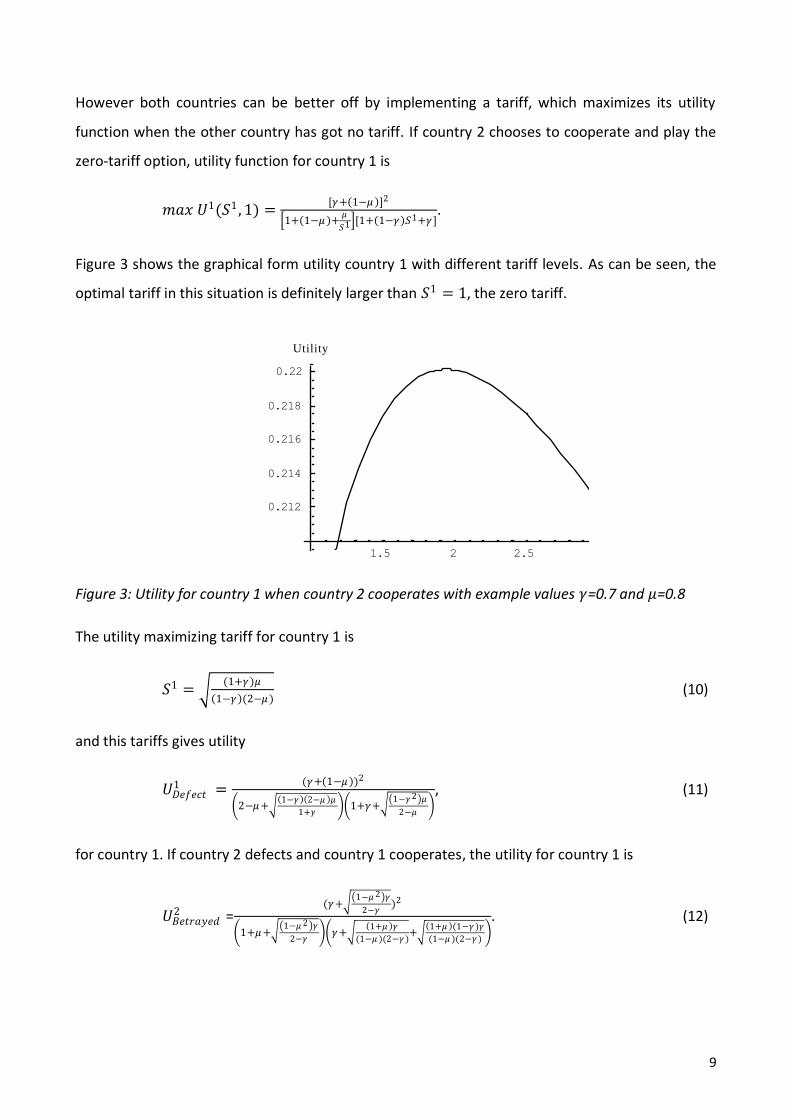
However both countries can be better off by implementing a tariff, which maximizes its utility

function when the other country has got no tariff. If country 2 chooses to cooperate and play the

zero-tariff option, utility function for country 1 is

𝑚𝑎𝑥 𝑈1(𝑆1 , 1) =[𝛾+ 1−𝜇 ]2

1+ 1−𝜇 +𝜇

𝑆1 [1+ 1−𝛾 𝑆1+𝛾].

Figure 3 shows the graphical form utility country 1 with different tariff levels. As can be seen, the

optimal tariff in this situation is definitely larger than 𝑆1 = 1, the zero tariff.

Figure 3: Utility for country 1 when country 2 cooperates with example values 𝛾=0.7 and 𝜇=0.8

The utility maximizing tariff for country 1 is

𝑆1 = (1+𝛾)𝜇

1−𝛾 (2−𝜇 ) (10)

and this tariffs gives utility

𝑈𝐷𝑒𝑓𝑒𝑐𝑡1 =

(𝛾+ 1−𝜇 )2

2−𝜇+ 1−𝛾 2−𝜇 𝜇

1+𝛾 1+𝛾+

1−𝛾2 𝜇

2−𝜇

, (11)

for country 1. If country 2 defects and country 1 cooperates, the utility for country 1 is

𝑈𝐵𝑒𝑡𝑟𝑎𝑦𝑒𝑑2 =

(𝛾+ 1−𝜇 2 𝛾

2−𝛾)2

1+𝜇+ 1−𝜇 2 𝛾

2−𝛾 𝛾+

1+𝜇 𝛾

(1−𝜇 )(2−𝛾 )+

1+𝜇 (1−𝛾 )𝛾

(1−𝜇 )(2−𝛾 )

. (12)

1.5 2 2.5 3Tariff

0.212

0.214

0.216

0.218

0.22

Utility

10

At the Nash equilibrium neither country can get more profit by changing its tariff level according

to the definition in chapter 3.1. Country 1 maximizes its utility (8) given all the optimal responses

of country 2, and as a result we get the Nash equilibrium tariffs that are

𝑆1 = 𝜇

1−𝛾, 𝑆2 =

𝛾

1−𝜇 (13)

which equal the offer curve elasticities as McMillan points out using a different approach [13].

Figure 4 shows utilities for different tariffs when country 2 implements an equilibrium tariff.

Figure 4: Utility for country 1 when country 2 chooses Nash equilibrium tariff with example values

𝛾=0.7 and 𝜇=0.8

Country 1 maximizes its utility by implementing a Nash equilibrium tariff by which country 1 gets

utility

𝑈𝑁𝑎𝑠ℎ1 =

(𝛾+ 1−𝜇 𝛾)2

𝛾+ 𝛾

1−𝜇+

1−𝛾 𝛾𝜇

1−𝜇 1+ 𝛾−𝛾𝜇 + 𝜇−𝛾𝜇

. (14)

The solution for a one-shot game like this is the Nash equilibrium, because Inequality 𝑈𝐵𝑒𝑡𝑟𝑎𝑦𝑖 ≥

𝑈𝐹𝑇𝑖 holds true in each point. This game is represented in a matrix form in Figure 5 where both

countries have two possible strategies: cooperate and defect. It is notable however, than

defection can mean either tariff (10), if (cooperate, cooperate) was played in previous game, or

tariff (13) if (cooperative, defect) or (defect, defect) was played before. If 𝑈𝐹𝑇𝑖 > 𝑈𝑁𝑎𝑠ℎ

𝑖 , i=1,2, the

game is a Prisoner’s dilemma. Otherwise (defect, defect) is not just Nash equilibrium, but also the

best alternative for both countries.

1.5 2 2.5 3Tariff

0.166

0.168

0.172

0.174

0.176

Utility

11

Country 2

Cooperate Defect

Country 1 Cooperate 𝑈𝐹𝑇1 , 𝑈𝐹𝑇

2 𝑈𝐷𝑒𝑓𝑒𝑐𝑡1 , 𝑈𝐵𝑒𝑡𝑟𝑎𝑦

2

Defect 𝑈𝐷𝑒𝑓𝑒𝑐𝑡

1 , 𝑈𝐵𝑒𝑡𝑟𝑎𝑦𝑒𝑑2 𝑈𝑁𝑎𝑠ℎ

1 , 𝑈𝑁𝑎𝑠ℎ2

Figure 5: Game in a matrix form

3.4 Nash equilibrium of a repeated game

In a repeated game Figure 4 is played multiple times in a row, and decisions made in previous

periods affects on present actions of the another country. Each country chooses a strategy, which

in dynamic game means “a complete plan of action-it specifies a feasible action for player in every

contingency in which player might be called upon to act”, as Gibbons defines it [7]. If each agent

can observe other agents’ actions and react to them, it is possible to reach a cooperative

equilibrium according to Folk-theorem [7]. For simplicity we assume that each country cooperates

in the beginning, but as soon as the other player defects, it reacts by permanent retaliation. This is

the Grim Trigger Strategy, so called because no matter what, (cooperate, cooperate) will never be

played again after defection [2].

We use the standard assumption that the utility gained later is less important than the utility

gained now. Since utilities (2) are monetary, the price for delayed consumption is assumed to

equal the missed investment opportunities, which can be calculated using the interest rate 𝑟𝑖 in

country i. Let’s assume that in each round there is a breakdown probability p for an instant stop of

trade, for example due to political reasons. The probability that the game lasts for another round

is thus (1 − 𝑝). If p is zero the game is called infinitely repeated game, but if p > 0 it is called

finitely repeated game. The discount rate is

𝛿𝑖 =1−𝑝

1+𝑟𝑖, (15)

for country i. Country 1 will cancel the free trade agreement, if its sum of discounted utility is

higher that way. Because of the grim trigger strategy, a tariff leads to a retaliation action by

12

another country, and the Nash equilibrium is being played for the rest of the game. In

mathematical form, country i defects if

(𝛿𝑖)𝑗𝑈𝐷𝑒𝑓𝑒𝑐𝑡

𝑖𝑘𝑗=0 + (𝛿𝑖)

𝑗𝑈𝑁𝑎𝑠ℎ𝑖∞

𝑗=𝑘 ≥ (𝛿𝑖)𝑗𝑈𝐹𝑇

𝑖∞𝑗=0 , i=1,2 (16)

where k is the number of time periods it takes for another player to react and 𝛿𝑖 is the discount

rate.

Kennan and Reizman present a model in which the interest rate and the probability of a

breakdown equal zero. By this assumption the discount rate 𝛿 equals zero and inequality (16) can

be simplified to

𝑈𝑁𝑎𝑠ℎ𝑖 ≥ 𝑈𝐹𝑇

𝑖 , i=1,2 (17)

The trade war pays off if the Nash equilibrium utility is higher that the free trade utility. We get an

identical answer by assuming the reaction time to be zero. Utilities in (17) depend only on sizes of

countries as (9) and (14) reveal. Inequalities (17) are drawn in Figure 6. Defecting makes sense for

country 1 in bottom right corner and for country 2 in top left corner. Free trade takes place only in

the cigar-shaped area in which neither inequality holds true. As we see, the free trade is possible

and profitable only for countries of approximately equal size. The thin line connecting top left and

bottom right corners equals the case in which a country has equal amount of both goods and no

trade takes place.

13

Figure 6: Conditions for free trade when p=0 and 𝑟𝑖=0, i=1,2

Now consider a case where the discount rate does not equal one either because of the interest

rate, breakdown probability or both. The time has a value now, and defecting becomes more

interesting option for both countries. We assume that the interests are paid monthly, and one

time period in (16) is one month. We also assume that the reaction time for defection is exactly

one month, k=1. Following these assumptions and using geometric sums (16) can be reduced to

𝑈𝐷𝑒𝑓𝑒𝑐𝑡1 +

𝛿

1−𝛿𝑈𝑁𝑎𝑠ℎ

1 ≥1

1−𝛿𝑈𝐹𝑇

1 . (18)

Without breakdown probability and with interest rate of 10% in both countries, the free trade

area becomes slightly thinner. However this interest rate does not change the outcome very

much.

14

Figure 7: Conditions for free trade when p=0 and 𝑟𝑖=0.1, i=1,2

Now consider the trade in politically unstable environment. Interest rate is assumed to be zero,

but the risk of war increases breakdown probability to 30 % in one month. Increased possibility of

breakdown increases the discount rate and reduces the size of free trade area.

15

Figure 8: Conditions for free trade when p=0.3 and r=0

If discount rate (15) is high enough, no free trade will ever occur.

4. Example: The Transatlantic Free Trade Union

The rise of new economic powers with comparative advantage in labor-intensive industries, such

as China or India, are forcing Europe and America to find more efficient ways to trade in order to

compete. One of the suggested proposals is a so-called Transatlantic Free Trade Area (TAFTA),

which would eliminate all the tariffs between EU and USA and their existing free trade partners

[5]. This would be beneficial for Western world as a whole as theory of comparative advantage

tells, but it is sustainable only if it is beneficial for both participants.

Consider a world of only two actors, Western Europe and North America, and two goods, steel and

agricultural products. In 2001, 64.7 % of all the steel came from Western Europe while the

equivalent number for North America was 35.3 % [15]. North America has a comparative

advantage in land-intensive agricultural products. It holds 69.4 % of all the agricultural products in

the world including wheat, coarse grains, rise and oilseeds [18]. In January 2001 the real interest

16

rate was 2.7 % in Europe and in USA it is 1.9 % in USA [17]. Since there are no political problems

between Europe and North America, the risk for breakdown of the agreement is approximately

zero.

We assume that the free trade area has been created, and a repeated game starts. At the free

trade all tariffs are zero, but if either agent decides to defect, it chooses tariff (10). The optimal

tariff for Europe is 57.5 % and for USA 62.7 %, and it gives defecting agent a non-recurring utility.

After this other player retaliates, and Nash equilibrium tariffs (13) will be 45.4 % for Europe and

40.2 % for USA. As can be seen, the defection tariff is higher than the Nash equilibrium. The area

in which free trade is sustainable is drawn in Figure 9. The TAFTA point 𝛾=0.647, 𝜇=0.694 is within

the grey area, so the free trade agreement would be sustainable if all other things stay equal.

Figure 9: Conditions for Transatlantic Free Trade Area

It is interesting to examine how much the initial values will have to change to start a trade war. To

do this we solve the equation

17

(𝛿𝑖)𝑗𝑈𝐷𝑒𝑓𝑒𝑐𝑡

𝑖𝑘𝑗=0 + (𝛿𝑖)

𝑗𝑈𝑁𝑎𝑠ℎ𝑖∞

𝑗=𝑘 = (𝛿𝑖)𝑗𝑈𝐹𝑇

𝑖∞𝑗=0 (19)

numerically for each constant to find limit values for free trade stability.

The limit value for breakdown probability is 0.416. This means that neither country will break the

agreement unless the risk of breakdown in next month is 41.6 %. The high number signals high

stability of this free trade agreement. The limit values for real interest rates in USA and Europe are

74.4 % and 76.4 %. This high real interest rate values can never be reached, so changes in real

interest rate don’t have effect on the stability of this equilibrium. If the market sizes of countries

change radically there might be an intensive to break the agreement. Limit value Europe’s part of

steel markets are 86.4 % and 50.2 % and for values for America’s part of agricultural products 45.7

% and 82.6 %. In other words Europe’s steel proportion has to increase 21.7 or decrease 14.5

percentage units, or America’s agriculture proportion has to increase 13.6 or decrease 23.3

percentage units so that free trade would not be the optimal solution for both countries.

Even though TAFTA seems to be beneficial for both countries and almost immune for changes in

political situation, real interest rates or changes in market proportions, first steps for reaching it

are still yet to be made. Reasons are mostly non-economical, and one of them lies in politics:

France has traditionally valued continental relations over trans-Atlantic connections. In America,

many politicians oppose the North American Free Trade Area, and it would be hard for them to

accept a new, even larger Free Trade agreement. The model used in this chapter is simple and

somewhat inaccurate. It reduces the trade between USA and EU in two goods although they make

just a small share of the total trade. However they set an example of how the trade works, and the

model could be expanded if more data was available.

5. Conclusion

In this paper we gave a brief review on the topic and on previous theories. In addition to that we

developed a model which takes the interest rate and the breakdown probability into account

while measuring the conditions for free trade. This model had two interesting results. Firstly, the

increase in interest rate makes the free trade area thinner, but with normal interest rate values

the change is quite small. In other words, the role of fluctuation in interest rate is very small in

free trade conditions. Secondly, a big increase in breakdown probability reduces the free trade

18

area, and might cause the abolition of the agreement. If this probability is high enough, the area

might even disappear. This predicts that free trade areas are rarer in politically unstable areas.

The model does not fully represent real world and some of the assumptions might have simplified

the model too much. In the real world countries have more than just one trading partner, and if

one country imposes a tariff, this good can be bought from a third party. Even though it is still

possible to win trade wars as pointed out by Kreinin, Dinopoulos and Constantinos (1996), the

presence of third country probably affects on the free trade conditions [11]. Countries produce

more than one good and if consumers appreciate some goods more than others, the Cobb-

Douglas utility function assumption (2) is wrong. Also all governments do not aim to maximize the

welfare of their citizens and this model is suitable only to examine actions of western

democracies.

This model could be developed in many ways. It would be interesting to examine a multi-country

model to see whether it makes free trade more or less probable. In this model only tariff was

examined because of its mathematical simplicity, but it would be interesting to see effects of trade

quotas and subsidies as well. We assumed that every country uses a grim trigger strategy, but in

real life countries will probably not retaliate forever, but aim to arrange a new free trade pact one

day. Different strategies will affect on the conditions and it would be interesting topic of research

to find out how.

References

[1] Antweiler W., Copeland B.R. & Taylor M.S.: “Is Free Trade Good for the Environment?”,

American Economic Review, 2001, pp. 877-908

[2] Axelrod, R: “On Six Advances in Cooperation Theory”, 2000

[3] Baldwin, R.E.: “The Case against Infant-Industry tariff protection”, The Journal of Political

Economy, Volume 77, No.3, 1969, pp 295-305

[4] De Scitovszky, T: “A Reconsideration of the Theory of Tariffs”, The Review of Economic

Studies, Volume 9, No. 2, pp. 89-110, 1942

[5] Denman, R.: “A Trans-Atlantic Free Trade Area?”, New York Times, 1995

19

[6] Gandolfo G.: International Economics I: The Pure Theory of International Trade, 1987 pp. 7-23,

107-125

[7] Gibbons, R: Game Theory for Applied Economists, 1992, pp. 2-142

[8] Irwin, D.A.: “Free Trade Under Fire”, 2002, pp. 46-54

[9] Johnson H.G.: “Optimum Tariffs and Retaliation”, The Review of Economic Studies, Volume

21, No. 2, 1953-1954

[10] Kennan J. & Riezman R.: ”Do Big Countries Win Tariff Wars?”, International Economic

Review, p. 81-85, 1988

[11] Kreinin, M.E., Dinopoulos E, Constantinos S.: ”Bilateral Trade Wars”, International Trade

Journal, Volume 10, No.1, pp. 3-20, 1996

[12] Krugman, P: “Is Free Trade Passé”, The Journal of Economic Perspectives, Volume 1, No. 2,

1987, pp. 131-144

[13] McMillan, J: Game Theory in International Economics, 1986, pp. 1-42

[14] Naya J.M. & Naya L.M.: “Tariff Retaliation and the Free Trade Argument”, International

Game Theory Review, Volume 9, No. 4, pp. 657-666, 2007

[15] Schabrun, G: ”The Visible Hand of Steel Industry”, http://schabrun.com/#_Toc10565117,

2002.

[16] Syropoulos, C: “Optimum Tariffs and Retaliation Revisited: “How Country Size Matters”, The

Review of Economic Studies, Volume 69, pp. 707-727, 2002

[17] Weller C.E.: Cutting U.S. interest rates would give the European economy room to breathe,

http://www.epi.org/economic_snapshots/entry/webfeatures_snapshots_archive_06252003/, 2003

[18] World Agricultural Production Crop Production Tables, Table 2: World Summary,

http://www.fas.usda.gov/wap/circular/2001/01-01/tables.html, 2001