1

Free Trade Agreements and Sectoral Adjustments in East Asia*

Hiro Lee† Research Institute for Economics and Business Administration,

Kobe University, Kobe 657-8501, Japan

Dominique van der Mensbrugghe The World Bank, Washington, DC 20433, USA

May 2005

Abstract

Although East Asian countries were relatively inactive in signing free trade agreements (FTAs) until the end of 1990s, a number of FTAs involving East Asian countries have been signed since the turn of the century. Because sectoral interests can exert significant influence on policy negotiations, the sectoral results would be most important for political economy considerations. The objective of this study is to evaluate the sectoral adjustments resulting from various FTA scenarios in East Asia using a dynamic global CGE model. Among other issues, the indices of revealed comparative advantage (RCA) are computed and RCA rankings of commodities with various FTA scenarios and those with the global trade liberalization scenario are correlated to examine how “natural” the groupings would be. JEL classification codes: F13, F15 Keywords: FTA, RCA, East Asia, CGE model

1. Introduction

In the past decade the number of free trade agreements (FTAs) has proliferated

rapidly. Other than ASEAN Free Trade Agreement (AFTA), East Asian countries were

relatively inactive in signing FTAs until the end of 1990s. Since 2001, however, a number

of FTAs involving East Asian countries have been signed or ratified: Singapore-New

Zealand (2001), Japan-Singapore (2002), ASEAN-China (2002), U.S.-Singapore (2003),

Singapore-Australia (2003), Korea-Chile (2004), Thailand-Australia (2004), Japan-

* Since this is a very preliminary and incomplete version, please do not quote. † Corresponding author. E-mail: hlee@rieb.kobe-u.ac.jp; tel.: +81-78-803-7023; fax: +81-78-803-7059.

2

Mexico (2004), and Korea-Singapore (2004). Japan and the Philippines have reached basic

agreement to conclude an FTA in 2005, and a large number of FTAs are currently being

negotiated in East Asia, including ASEAN-Japan, ASEAN-Korea, Japan-Korea, and

Japan-Thailand. The ASEAN+3 group, consisting of the ASEAN countries, China, Japan,

and Korea, has provided an effective mechanism for greater cooperation and gradual

regional economic integration in East Asia. The trends in negotiating for new FTAs are

likely to continue in East Asia.

Whether regional integration agreements (RIAs) are a facilitating intermediate step

towards global free trade or a hindrance to greater global trade liberalization is a hotly

debated issue (e.g., Krueger, 1999a; Laird, 1999; Panagariya, 2000). Proponents for

regional integration argue that RIAs encourage member countries to liberalize beyond the

level committed by multilateral negotiations and that they make tough negotiating issues

easier to handle (e.g., Kahler, 1995). In addition, RIAs are likely to induce dynamic effects

that might contribute to member countries’ growth through the accumulation of physical

and human capital, productivity growth, and accelerated domestic reforms (e.g., Ethier,

1998; Fukase and Winters, 2003).1 Opponents worry that the proliferation of RIAs is

likely to undermine the multilateral trading system and that beneficiaries of RIAs might

form a political lobby to deter further multilateral liberalization (e.g., Bhagwati, 1995;

Levy, 1997; Srinivasan, 1998ab; Panagariya, 1999).

Empirical evidence on benefits and costs of RIAs suggests that trade creation

exceeds trade diversion in almost all RIAs (Robinson and Thierfelder, 1999). The positive

effect on economic welfare resulting from the European Union (EU) and North American

Free Trade Agreement (NAFTA) is supported by Brown, Deardorff, and Stern (1992),

Harrison, Rutherford, and Tarr (1996), Lee and van der Mensbrugghe (2004), and Roland-

Holst, Reinert, and Shiels (1992). However, Yeats (1998) finds that during 1988-94

Mercosur countries experienced significant trade diversion when their intra-Mercosur

trade increased sharply.

While the aggregate welfare effect of FTAs is certainly important, the sectoral

impact could be of an even greater concern to policy makers. This is because regional

1 Ethier (1998) suggests that small-country members are induced to lock in their liberalized trade regimes and that RIAs are congruent with further multilateral liberalization.

3

integration might lead to a sharp contraction of output and employment in highly protected

sectors. For example, the agricultural sectors in Japan and Korea are highly subsidized

and shielded against foreign imports by significant tariffs and nontariff barriers (NTBs). In

a number of developing members, tariffs, industrial policy, and other government policies

protect certain manufacturing industries from foreign competition. Since trade policy is

often formulated from the bottom up, a modern view of national interest, such as that

based on trade reciprocity, might encounter conflicts with established domestic interests.

Using a dynamic global computable general equilibrium (CGE) model, we

evaluate the effects of prospective free trade agreements involving East Asian countries,

emphasizing sectoral adjustments and changes in the pattern of trade resulting from the

formation of FTAs. The next section gives an overview of the model. Section 3 provides a

brief description of scenarios and assessments of computational results. The final section

summarizes the main policy conclusions.

2. Overview of the Model

The model used in this study, known as the LINKAGE model, is a dynamic global

CGE model developed by van der Mensbrugghe (2004).2 It spans the period 1997-2015 in

the present version and is a relatively standard neoclassical CGE, with constant returns to

scale in all sectors, perfect competition and price-clearing behavior in all markets. The

model incorporates three types of production structure—crops, livestock, and

manufacturing and services. The first distinguishes intensive (chemical- and labor-based)

farming versus extensive (land-based) farming. Livestock production is characterized by

ranch- versus range-fed cattle. All other sectors conform to the more standard labor-capital

substitution effects, albeit with sufficient structure to capture the complex interactions

across various inputs and factors of production (see Figure 1).3

2 See van der Mensbrugghe (2005) for the model equations. This section largely replicates Lee, Roland-Holst, and van der Mensbrugghe (2004, section 2), but will be updated in a revised version. 3 At the top nest, production is formed by the combination of aggregate intermediate demand other than energy (ND) and value added plus energy (VA). The second nest consists of two nodes. The first node decomposes aggregate intermediate demand into sectoral demand for goods and services. The second node decomposes VA between demand for aggregate labor (L) and demand for human capital, physical capital, energy, and sector-specific factor bundle (HKTE). The third and subsequent nodes are decomposed by a similar fashion, as illustrated in Figure 1.

4

Figure 1 Production nesting in the manufacturing and services sectors

XP: Output

ND: Aggregate intermediate demand VA: Value added plus energy

XAp: Intermediate demand

XD: Demand for domestic goods

XMT: Aggregate import demand

WTF: Demand by region of origin

AL: Labor demand

Unkilled Skilled

HKTE bundle

HKT bundle XEp: Energy bundle

KT bundle Highly skilled

By type of energy

By region of origin…

σ p

Sector-specific factor

σ v

σ e

σ hσ ep

σ m

σ w

σ l

σ = 0

σ k

Capital

5

Figure 1 (continued) Definition of variables and parameters:

XP: Output (by vintage) ND: Demand for aggregate non-energy intermediate demand VA: Demand for labor, capital, energy, and sector-specific factor bundle XAp: Demand for (Armington) intermediate goods (excluding energy) XD: Demand for domestically produced intermediate goods XMT: Aggregate import demand for intermediate goods WTF: Demand for imported intermediate goods by region of origin AL: Demand for aggregate labor (excluding ‘highly’ skilled) HKTE: Demand for human and physical capital, energy, and sector-specific factor bundle XEp: Demand for aggregate energy bundle HKT: Demand for human capital, physical capital, and sector-specific factor bundle KT: Demand for physical capital and sector-specific factor bundle σp: Elasticity of substitution between ND and VA σv: Elasticity of substitution between AL and HKTE σl: Elasticity of substitution between unskilled and skilled labor σe: Elasticity of substitution between XEp and HKT σep: Elasticity of substitution between different type of energy σh: Elasticity of substitution between KT and highly skilled labor σk: Elasticity of substitution between physical capital and sector-specific factor

Note: The sector-specific factor includes land in agricultural sectors and the resource base in the coal, crude oil, natural gas, and mining sectors.

Factor income accrues to a single representative household, which finances

government expenditures (through direct and indirect taxes) and investment (through

domestic savings). Domestic savings may be augmented or diminished by a net capital

flow. In the current version of the model, the latter is exogenous in any given time period

for each region, thereby generating a fixed current account balance. Ex ante shocks to the

current account—e.g., a reduction in trade barriers—induces a change in the real exchange

rate. Government fiscal balances are also fixed in each time period, and the equilibrating

mechanism is lump-sum taxes on the representative household. For example, a reduction

in tariff revenue is compensated by an increase in household direct taxation.

Trade is modeled using the ubiquitous Armington assumption of imperfect

substitution, i.e., goods are differentiated by region of origin. The model uses a nested

demand structure. Aggregate domestic absorption by sector is allocated between domestic

goods and a single composite import good. The latter is then allocated across region of

origin to determine the bilateral trade flows on a sectoral basis. An analogous dual-nested

structure is used to allocate domestic production between domestic and export markets

(using constant elasticity of transformation functions).

6

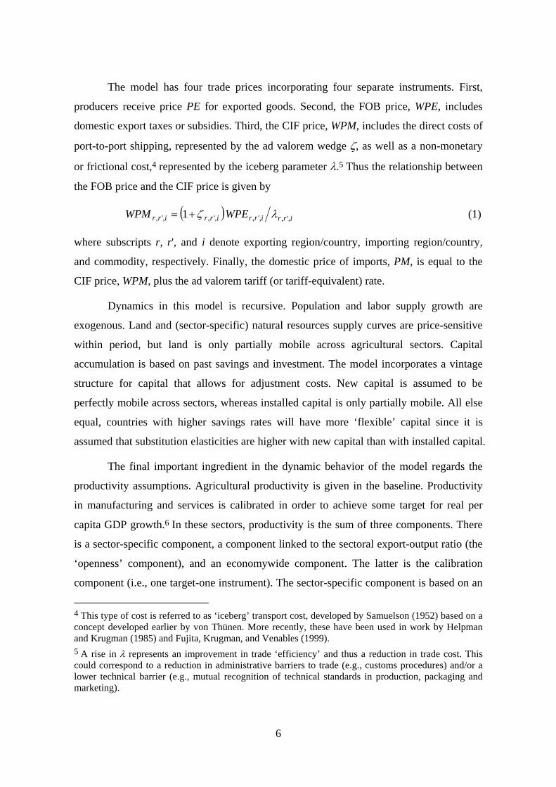
The model has four trade prices incorporating four separate instruments. First,

producers receive price PE for exported goods. Second, the FOB price, WPE, includes

domestic export taxes or subsidies. Third, the CIF price, WPM, includes the direct costs of

port-to-port shipping, represented by the ad valorem wedge ζ, as well as a non-monetary

or frictional cost,4 represented by the iceberg parameter λ.5 Thus the relationship between

the FOB price and the CIF price is given by

( ) irrirrirrirr WPEWPM ,',,',,',,', 1 λζ+= (1)

where subscripts r, r', and i denote exporting region/country, importing region/country,

and commodity, respectively. Finally, the domestic price of imports, PM, is equal to the

CIF price, WPM, plus the ad valorem tariff (or tariff-equivalent) rate.

Dynamics in this model is recursive. Population and labor supply growth are

exogenous. Land and (sector-specific) natural resources supply curves are price-sensitive

within period, but land is only partially mobile across agricultural sectors. Capital

accumulation is based on past savings and investment. The model incorporates a vintage

structure for capital that allows for adjustment costs. New capital is assumed to be

perfectly mobile across sectors, whereas installed capital is only partially mobile. All else

equal, countries with higher savings rates will have more ‘flexible’ capital since it is

assumed that substitution elasticities are higher with new capital than with installed capital.

The final important ingredient in the dynamic behavior of the model regards the

productivity assumptions. Agricultural productivity is given in the baseline. Productivity

in manufacturing and services is calibrated in order to achieve some target for real per

capita GDP growth.6 In these sectors, productivity is the sum of three components. There

is a sector-specific component, a component linked to the sectoral export-output ratio (the

‘openness’ component), and an economywide component. The latter is the calibration

component (i.e., one target-one instrument). The sector-specific component is based on an

4 This type of cost is referred to as ‘iceberg’ transport cost, developed by Samuelson (1952) based on a concept developed earlier by von Thünen. More recently, these have been used in work by Helpman and Krugman (1985) and Fujita, Krugman, and Venables (1999). 5 A rise in λ represents an improvement in trade ‘efficiency’ and thus a reduction in trade cost. This could correspond to a reduction in administrative barriers to trade (e.g., customs procedures) and/or a lower technical barrier (e.g., mutual recognition of technical standards in production, packaging and marketing).

7

aggregate assumption, typically that productivity is some percentage point higher in

manufacturing than in services (e.g., 2 percentage points). The openness component is

calibrated in the baseline so that it explains a specified share of total sectoral productivity.

In policy reforms scenario, this component (χi,t) is assumed to be endogenous, i.e., it

changes with the ratio of exports to output:

i

ti

tititi X

Eη

φχ ⎟⎟⎠

⎞⎜⎜⎝

⎛=

,

,,, (2)

where Ei,t is exports of commodity i, Xi,t is output of commodity i, φi,t is a shift parameter,

and ηi is the elasticity of productivity with respect to openness. For example, if

manufacturing productivity in the baseline is 4 percent in some year, the openness

component explains 50 percent of total sectoral productivity, and the export-output ratio

increases by 10 percent, then productivity would increase by 5 percent (to 4.2 percent)

assuming the openness elasticity is one.7

Previous studies have shown that two additional factors that are not incorporated in

the present model would significantly boost the gains from trade. First, Harris (1984),

Brown and Stern (1989), and Francois and Roland-Holst (1997), among others, have

demonstrated that incorporation of increasing returns to scale and imperfect competition

could lead to multiple changes in the aggregate results. Second, foreign capital flows (e.g.,

foreign direct investment and portfolio investment) are exogenous in the current version of

the model, but it has been shown that allowing for capital to flow to countries with

relatively high rates of return could significantly raise the gains from trade reform.8

6 Productivity is assumed to be labor-augmenting. 7 Note that if the export-output ratio increases by 10 percent, then assuming ηi = 1 the openness component of productivity, χi,t, increases by 10 percent. Since the other two components of productivity are exogenous, an increase in sectoral productivity is calculated as [θχ (1 + gχ) + (1 – θχ)] – 1 = [0.5*(1 + 0.10) + (1 – 0.5)] – 1 = 0.05 where θχ is the share of sectoral productivity explained by the openness component and gχ is the rate at which χi,t increases. 8 See, for example, Petri (1997) and Lee and van der Mensbrugghe (2001).

8

Table 1. Regional and Sectoral Aggregation A. Regional Aggregation Countries/Regions Corresponding economies/regions in the GTAP database China China and Hong Kong Japan Japan Korea Korea Taiwan Taiwan ASEAN Indonesia, Malaysia, Philippines, Singapore, Thailand, Vietnam, rest of Southeast Asia Australasia Australia and New Zealand North America United States, Canada, Mexico Latin America Central America and the Caribbean, South America EU-25 Austria, Belgium, Denmark, Finland, France, Germany, Great Britain, Greece, Ireland, Italy, Luxembourg, Netherlands, Portugal, Spain, Sweden, plus the ten new member countries Rest of world All the other economies/regions

B. Sectoral Aggregation Sectors Corresponding commodities/sectors in the GTAP database Rice Paddy rice, processed rice Other grains Wheat, cereal grains n.e.s. Vegetables and fruits Vegetables and fruits Other crops Oil seeds, sugar cane and sugar beet, plant-based fibers, crops n.e.s. Livestock Bovine cattle, sheep and goats, animal products n.e.s. Natural resources forestry, minerals Fossil fuel Coal, oil, gas Food Fishing, food products, beverages and tobacco products Textiles Textiles Apparel Wearing apparel Leather Leather products Wood products Wood products Paper products Paper products publishing Petroleum products Petroleum and coal products Chemicals Chemical, rubber, plastic products Mineral products Non-metallic mineral products Iron and steel Iron and steel Nonferrous metal Nonferrous metal Metal products Fabricated metal products Machinery Machinery and equipment Electronic equip. Electronic equipment Motor vehicles Motor vehicles and parts Other transport equip. Other transport equipment Other manufactures Manufactures n.e.s. Trade and transport Trade, sea transport, air transport, transport n.e.s. Services Construction, public utilities, communication, financial services, other services Source: GTAP database, Version 6 (Beta Release).

9

Most of the data used in the model come from the Beta Release of the GTAP

database, version 6, which provides 2001 data on input-output, value added, final demand,

bilateral trade, tax and subsidy data for 87 regions and 57 sectors.9 For the purpose of the

present study, the database is aggregated into 10 regions and 26 sectors as shown in Table

1.

3. Scenarios and Results

3.1 Policy Scenarios

To evaluate sectoral adjustments and changes in the pattern of trade resulting prospective free trade agreements in East Asia, the following six policy scenarios are considered:

1) ASEAN-China FTA: Free trade among the ASEAN countries and China/Hong

Kong

2) ASEAN-Japan FTA: Free trade among the ASEAN countries and Japan

3) China-Japan-Korea FTA: Free trade among China/Hong Kong, Japan, and Korea

4) ASEAN+3: Free trade among the ASEAN countries, China/Hong Kong, Japan, and Korea

5) ASEAN-EU: Free trade among the ASEAN and EU-25 member countries

6) Global trade liberalization (GTL): Complete abolition of import tariffs and export

subsidies

While the likelihood of actually completing the above trade liberalization or FTAs within

a reasonable time horizon differs significantly across scenarios, it is worth examining each

of them. Scenario 1 is expected to be realized as ASEAN countries and China signed a

framework agreement in 2002 to establish the FTA for trade in goods by 2010 for China

and ASEAN-6 and by 2015 for newer ASEAN Member States.10 Scenario 2 that excludes

9 Dimaranan and McDougall (forthcoming) give detailed descriptions of the GTAP database, version 6. 10 ASEAN-6 refers to the original ASEAN members; i.e., Brunei, Indonesia, Malaysia, Philippines, Singapore, and Thailand. Newer ASEAN Member States are Cambodia, Lao PDR, Myanmar, and Vietnam.

10

sensitive sectors has also become a real possibility after ASEAN and Japan signed an

agreement on the Comprehensive Economic Partnership (CEP) in November 2003.11 The

proposal for China-Japan-Korea FTA (scenario 3) has been considered by the

governments of the three countries (Wong et al., 2004), and a joint research on economic

cooperation among these countries has been undertaken by the Development Research

Center of the State Council of China, the National Institute for Research Advancement of

Japan, and the Korea Institute for International Economic Policy. Although negotiations

for an FTA among the economies of ASEAN+3 have not yet begun, we include scenario 4

because a number of studies have examined the possible effects of such an arrangement

(e.g., Brown, Deardorff, and Stern, 2003; Lee and Park, 2005). In addition, since EU has

established a cooperative relationship with ASEAN, it would be natural to consider

scenario 5 in which ASEAN and the EU form an FTA. Finally, we have the global trade

liberalization (GTL) or full WTO scenario so that the effects of the FTA scenarios may be

discussed relative to the global scenario.

In all FTA experiments, we gradually remove bilateral tariffs and export subsidies

of the relevant sectors among the member countries over the 2007-2012 period. We set the

elasticity of productivity with respect to openness, ηi, to 0.5 in agricultural sectors and to

1.0 in all other sectors. We assume that non-monetary trade costs would be reduced by 2

percent in all FTA scenarios, but they remain unchanged in the unilateral and global

scenarios (scenarios 1 and 7).12

3.2 Effects on Welfare

Aggregate income gains and/or losses summarize the extent trade distortions are

hindering growth prospects and the ability of economies to use the gains to help those

whose income could potentially decline. We compare the six policy scenarios with the

11 Yamazawa and Hiratsuka (2003) provides an overview of ASEAN-Japan Comprehensive Economic Partnership. 12 Smith and Venables (1988) use a 2.5 percent reduction in intra-EU trade costs in their study of the Single Market program’s possible pro-competitive effects, whereas Keuschnigg and Kohler (2000) and Madsen and Sorensen (2002) use a 5 percent reduction in real costs of trade between the EU and Central and East European countries. We use a smaller reduction in these costs among the members of FTAs in scenarios 2-6 because the reductions in technical barriers are expected to be smaller in these cases than in the EU case.

11

baseline situation in the terminal year, 2015, using a measure of compensated or

equivalent variation aggregate national income. Real income is summarized by Hicksian

equivalent variation (EV). This represents the income consumers would be willing to

forego to achieve post-reform well-being (up) compared to baseline well-being (ub) at

baseline prices (pb):

( ) ( )bbpb upEupEEV ,, −= (3)

where E represents the expenditure function to achieve utility level u given a vector of

prices p (superscript b represents baseline levels, and p the post-reform levels). The model

uses the extended linear expenditure system (ELES), which incorporates savings in the

consumer’s utility function. The ELES expenditure function is easy to evaluate at each

point in time.

Table 2 summarizes the welfare results for the seven policy scenarios as deviations

in EVs from the baseline in 2015. The GTL or full WTO scenario (scenario 6) is the most

attractive for all countries and regions. To be realistic, however, the WTO process is

fraught with uncertainty about the scope, depth, and timeliness of multilateral

commitments to abolish trade barriers.13 This kind of uncertainty has been an important

impetus to regional agreements, particularly those between small groups of nations who

find consensus, implementation, and monitoring easier.

In the ASEAN-China FTA scenario (scenario 1), in 2015 EV of ASEAN increases

by 2.5%, whereas EV of China increases by a smaller percentage (1.0%). This largely

results from two factors: (1) the share of ASEAN’s exports to China is significantly larger

than the share of China’s exports to ASEAN; (2) the exports to output ratio is substantially

higher for ASEAN countries. The welfare effects on non-member countries are negligible

except for Korea and Taiwan, which experience 0.2 and 0.3 percent declines in their EVs.

When ASEAN and Japan form an FTA (scenario 2), ASEAN’s EV increases by 1.5

percent while Japan’s EV increases by 0.5 percent. Welfare of other East Asian countries

(China, Korea, and Taiwan) declines slightly.

13 See, for example, Langhammer (2004) for causes and triggers of the setback at the WTO Ministerial Conference in Cancún in September 2003.

12

Table 2 Effects on welfare (deviations in equivalent variations from the baseline in 2015) FTA and GTL Scenarios (1) (2) (3) (4) (5) (6) Region ASEAN- ASEAN- China- ASEAN ASEAN- GTL China Japan Japan-Korea plus 3 EU A. Absolute deviations (US$ billion in 2001 prices) China and Hong Kong 23.6 -2.8 61.8 56.6 -2.1 88.8 Japan -1.7 18.8 32.4 27.1 -0.4 53.7 Korea -1.0 -0.8 33.9 31.3 -0.7 45.5 Taiwan -1.1 -0.7 -1.3 -2.1 -0.5 10.2 ASEAN 24.3 14.5 -4.5 12.9 14.2 25.2 Australia/New Zealand -0.2 -0.2 -0.6 -0.8 -0.2 9.9 North America -0.3 -0.9 -0.3 -1.0 0.2 111.9 Latin America -0.1 -0.3 -1.7 -1.9 -0.7 31.6 EU-25 -1.8 -0.8 2.2 1.2 70.6 67.6 Rest of the world -1.7 -1.5 1.5 -0.4 -6.0 97.5 East Asia total 44.2 29.0 122.3 125.9 10.6 223.3 World total 40.1 25.2 123.4 123.1 74.5 541.8 B. Percent deviations China and Hong Kong 1.0 -0.1 2.5 2.3 -0.1 3.6 Japan 0.0 0.5 0.8 0.7 0.0 1.4 Korea -0.2 -0.1 5.0 4.7 -0.1 6.8 Taiwan -0.3 -0.2 -0.3 -0.5 -0.1 2.5 ASEAN 2.5 1.5 -0.5 1.4 1.5 2.6 Australia/New Zealand 0.0 0.0 -0.1 -0.2 0.0 2.0 North America 0.0 0.0 0.0 0.0 0.0 0.8 Latin America 0.0 0.0 -0.1 -0.1 0.0 1.9 EU-25 0.0 0.0 0.0 0.0 0.9 0.8 Rest of the world 0.0 0.0 0.0 0.0 -0.2 2.6 East Asia total 0.5 0.3 1.4 1.5 0.1 2.6 World total 0.1 0.1 0.3 0.3 0.2 1.5

When a free trade area is formed among China, Japan, and Korea (scenario 3),

Korea is expected to accrue the greatest welfare gain of 5.0 percent, following by China

(2.5 percent) and Japan (0.8 percent). This is largely because Korea will have preferential

accesses to the large Chinese and Japanese markets and its exports to China and Japan,

which already constitute large shares of Korea’s total exports, will increase dramatically.

Under the trilateral FTA, Korea, China, and Japan respectively obtain about 75, 70, and 60

percent of the GTL’s benefits. Thus, the China-Japan-Korea FTA could be a very

attractive stepping stone to globalization for the three countries although large political

obstacles must be surmounted to achieve such an FTA.

13

Under the ASEAN+3 FTA scenario (scenario 4), the welfare of all members

increases although the welfare gains for China, Japan, and Korea are somewhat smaller

than under the trilateral FTA. These losses are more than offset by the ASEAN’s gains and

East Asia as a whole is expected to gain $126 billion (1.5%) in 2015, compared with its

$223 billion (2.6%) gain under the GTL. In other words, East Asia will be able to attain 56

percent of GTL’s benefits from the ASEAN+3 FTA.

If free trade between ASEAN and the EU is realized (scenario 5), ASEAN is

expected to realize a 1.5 percent gain in its welfare, slightly larger than the gain expected

under the ASEAN+3 FTA scenario. The EU’s welfare will increase by 0.9 percent.

3.3 Effects on Sectoral Output

While the aggregate welfare and trade results are of interest in themselves, the

most useful results are at the industry level, where structural adjustments and resource

reallocations occur in response to policy changes. Because sectoral interests can exert

significant influence on policy negotiations, the sectoral results would be most important

for political economy considerations. In this section we examine the effects of alternative

policy scenarios on sectoral output.

Tables 3-6 summarize output adjustments for the 26 sectors in China and Hong

Kong, Japan, Korean, and ASEAN under the six policy scenarios. Sectoral adjustments are

expressed in percent deviations from the baseline for the year 2015. They are large in most

of the agricultural and food sectors for East Asia in general and Japan and Korea in

particular because of high trade barriers in these two countries.

[To be completed]

14

Table 3 China and Hong Kong’s sectoral output adjustments under alternative scenarios (percent deviations from the baseline for the year 2015) Scenarios (1) (2) (3) (4) (5) (6) Commodity/sector ASEAN- ASEAN- China- ASEAN ASEAN- GTL China Japan Japan-Korea plus 3 EU Rice 0.4 -0.3 25.3 22.6 0.0 21.6 Other grains 0.3 -0.1 34.6 33.7 0.2 -48.7 Vegetables and fruits 0.2 0.0 6.1 5.7 0.2 6.6 Other crops 0.0 -1.3 200.3 197.8 -1.1 1.4 Livestock 0.7 -0.1 3.0 3.0 -0.1 5.7 Natural resources -0.3 0.0 -0.9 -1.1 0.1 -2.6 Fossil fuel 0.3 0.1 0.0 0.1 0.2 -4.2 Food 1.3 -0.4 5.7 5.9 0.1 4.1 Textiles 0.9 -0.1 0.0 0.5 -0.9 11.2 Apparel -0.1 -0.1 4.9 3.5 -1.0 20.6 Leather 2.0 -0.2 2.5 2.8 -1.1 19.4 Wood products -1.4 0.2 0.6 -0.9 0.8 1.2 Paper products 0.1 0.1 0.0 0.2 0.2 0.0 Petroleum products 2.3 0.0 -0.9 1.1 0.0 -2.9 Chemicals -2.1 0.0 -0.5 -2.0 -0.1 -3.1 Mineral products 0.0 0.0 -0.5 -0.6 0.1 0.2 Iron and steel 0.7 -0.3 -1.9 -1.2 -0.1 -3.6 Nonferrous metal 0.1 -0.1 -2.3 -2.2 0.1 -6.6 Metal products 0.3 -0.2 -0.7 -0.6 -0.1 1.5 Machinery 0.4 -0.1 -1.3 -1.2 -0.1 -2.5 Electronic equip. 1.6 0.2 0.8 0.0 -0.2 2.7 Motor vehicles 2.0 -0.7 -4.2 -4.2 -0.8 -13.3 Other transport equip. 15.8 -0.4 0.1 14.3 -0.2 14.8 Other manufactures -0.4 0.1 -0.6 -0.8 0.2 -0.5 Trade and transport 0.0 0.1 0.1 0.0 0.3 0.4 Services 0.2 0.0 0.4 0.3 0.0 0.4 • China’s agricultural and food sectors expand under the China-Japan-Korea FTA and

ASEAN+3 FTA scenarios. In particular, the percentage increases in output of other crops are around 200 percent relative to the baseline in 2015 under these two scenarios.

• Among the manufacturing sectors, output of other transportation equipment increases

14-16 percent when the ASEAN countries are included in the FTA. • Output of the apparel and leather sectors increases moderately when Japan is an FTA

member (scenarios 3 and 4), but the increase is small relative to the GTL scenario because China’s exports of these products to Japan are relatively small compared with its exports to North American and the EU.

• The motor vehicle sector contracts when Japan and Korea are FTA members, but the

contraction is relatively small compared with the GTL scenario.

15

Table 4 Japan’s sectoral output adjustments under alternative scenarios (percent deviations from the baseline for the year 2015) Scenarios (1) (2) (3) (4) (5) (6) Commodity/sector ASEAN- ASEAN- China- ASEAN ASEAN- GTL China Japan Japan-Korea plus 3 EU Rice 0.4 -53.1 -74.8 -74.2 0.2 -79.8 Other grains 0.5 4.6 0.1 -1.4 0.4 -97.1 Vegetables and fruits 0.2 0.6 -0.7 -1.1 0.2 -5.8 Other crops 0.4 0.4 -3.3 -3.1 0.3 -7.8 Livestock 0.2 -0.9 0.5 -0.9 0.2 -6.7 Natural resources 1.2 -0.1 -0.6 0.3 0.7 -0.4 Fossil fuel 1.2 -1.9 -3.3 -2.6 0.7 -8.6 Food 0.1 -2.2 -3.2 -4.6 0.1 -15.5 Textiles -1.7 2.8 21.6 18.5 0.2 14.3 Apparel 0.2 -0.6 -7.0 -5.8 0.2 -7.7 Leather 0.5 -3.6 -11.7 -12.8 0.4 -21.2 Wood products 1.4 -0.9 -2.1 -1.1 1.0 -1.6 Paper products 0.1 0.0 -0.1 0.0 0.1 -0.5 Petroleum products -0.1 0.1 -0.1 -0.3 0.0 -3.5 Chemicals -0.6 0.6 2.3 1.6 0.0 1.4 Mineral products 0.0 0.5 2.7 2.7 0.0 2.6 Iron and steel 0.4 3.0 1.7 3.8 -0.4 3.9 Nonferrous metal 0.8 1.2 1.9 2.5 0.3 -0.1 Metal products 0.0 1.1 0.5 1.5 -0.1 1.9 Machinery 0.1 -0.2 3.0 2.4 -0.2 1.5 Electronic equip. -0.2 -0.8 -0.7 -1.4 0.5 -0.3 Motor vehicles -0.2 4.4 -0.5 3.0 -1.9 13.2 Other transport equip. -1.6 0.8 -2.8 -3.9 0.3 6.9 Other manufactures 0.6 0.7 -0.2 1.0 0.2 -0.2 Trade and transport 0.1 0.0 -0.1 -0.1 0.1 0.4 Services 0.0 0.2 0.3 0.2 0.0 0.5 • Japan’s rice sector contracts by 53-78 percent under the ASEAN-Japan FTA, China-

Japan-Korea FTA, and ASEAN+3 FTA scenarios. Compared with the GTL scenario, the contractions of other agricultural and food products, particularly other grains, are relatively small.

• Under the China-Japan-Korea FTA and ASEAN+3 FTA scenarios, the textile sector

expands by 19-22 percent while the apparel and leather sectors contract by 6-7 percent and 12-13 percent, respectively.

• Under the ASEAN+3 FTA scenario, output of steel increases by 3.8, almost the same

percentage increase as the GTL scenario largely because about three-quarters of Japan’s steel exports are shipped to other East Asian countries.

• Japan’s motor vehicle industry expands when ASEAN is included in the FTA, but

contracts slightly under the China-Japan-Korea FTA scenario.

16

Table 5 Korea’s sectoral output adjustments under alternative scenarios (percent deviations from the baseline for the year 2015) Scenarios (1) (2) (3) (4) (5) (6) Commodity/sector ASEAN- ASEAN- China- ASEAN ASEAN- GTL China Japan Japan-Korea plus 3 EU Rice 0.3 -0.1 425.4 392.4 -0.1 559.2 Other grains 0.9 -0.7 -99.8 -99.7 -0.4 -99.9 Vegetables and fruits 0.2 -0.2 -29.3 -27.8 0.1 -39.1 Other crops 0.6 -0.8 -43.9 -40.9 -0.4 -74.2 Livestock 0.0 -0.6 116.7 107.8 -0.1 119.2 Natural resources 2.0 0.3 -12.8 -12.2 0.5 -20.0 Fossil fuel 0.5 0.3 -4.0 -5.6 0.3 -18.1 Food 0.0 -0.8 100.3 90.8 0.0 106.8 Textiles -1.5 -0.3 8.2 10.5 -0.6 11.8 Apparel 1.2 0.3 -3.2 -2.3 0.1 -6.0 Leather -2.0 -0.4 79.9 72.0 -0.6 54.6 Wood products 1.8 0.7 -6.1 -9.0 1.1 -9.0 Paper products 0.4 0.3 -1.5 -2.6 0.4 -6.1 Petroleum products -2.1 -0.1 16.2 12.2 -0.1 21.5 Chemicals -3.0 -0.1 -1.0 -4.4 -0.2 -8.6 Mineral products 0.3 0.2 -6.4 -6.5 0.0 -13.1 Iron and steel 1.2 -0.9 -11.8 -9.8 -0.6 -15.1 Nonferrous metal 1.1 -0.2 -10.0 -7.6 -0.1 -17.8 Metal products 0.4 -0.4 -5.8 -5.3 -0.2 -7.6 Machinery 0.4 0.1 -12.3 -11.5 -0.1 -16.8 Electronic equip. 0.0 0.6 -8.8 -9.4 0.2 -11.3 Motor vehicles 0.7 -1.0 -9.2 3.7 -1.9 13.8 Other transport equip. -1.7 0.2 -20.3 -22.3 -0.4 5.8 Other manufactures 1.1 0.0 2.2 4.8 0.0 -5.4 Trade and transport 0.4 0.2 1.6 1.7 0.3 3.2 Services 0.0 0.0 1.1 0.9 0.1 1.5 • Under both FTA scenarios in which Korea is a member (i.e., scenarios 3 and 4),

Korea’s rice sector is expected to expand by about five-fold. The surge in rice output is driven by an extremely large increase in the exports to Japan.

• Large contractions in output of other grains, vegetables and fruits, and other crops, as

well as large expansions in output of livestock and processed food under the two FTA scenarios are consistent with sectoral adjustments of these sectors under the GTL scenario.

• Among the manufacturing sectors, output of textiles, leather, petroleum products, and

other manufactures would increase, but the motor vehicle industry is expected to contract under the China-Japan-Korea FTA scenario.

17

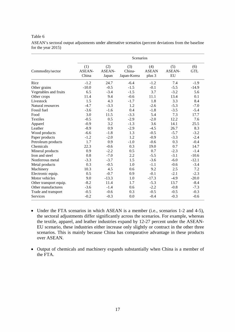
Table 6 ASEAN’s sectoral output adjustments under alternative scenarios (percent deviations from the baseline for the year 2015) Scenarios (1) (2) (3) (4) (5) (6) Commodity/sector ASEAN- ASEAN- China- ASEAN ASEAN- GTL China Japan Japan-Korea plus 3 EU Rice -1.2 24.7 -6.4 -1.2 7.4 -1.9 Other grains -10.0 -0.5 -1.5 -0.1 -5.5 -14.9 Vegetables and fruits 6.5 -3.4 -1.5 3.7 -3.2 5.6 Other crops 11.4 9.4 -0.6 11.1 13.4 0.1 Livestock 1.5 4.3 -1.7 1.8 3.3 8.4 Natural resources -4.7 -3.3 1.2 -2.6 -5.3 -7.0 Fossil fuel -3.6 -1.6 0.4 -1.8 -3.5 -5.4 Food 3.0 11.5 -3.3 5.4 7.3 17.7 Textiles -0.5 0.5 -2.9 -2.0 12.2 7.6 Apparel -0.9 3.2 -1.3 3.6 14.1 25.5 Leather -8.9 0.9 -2.9 -4.5 26.7 8.3 Wood products -6.6 -1.8 1.3 -0.5 -5.7 -3.2 Paper products -1.2 -2.0 1.2 -0.9 -3.3 -2.4 Petroleum products 1.7 0.9 -1.0 -0.6 0.3 -0.4 Chemicals 22.3 -0.6 0.3 19.0 0.7 14.7 Mineral products 0.9 -2.2 0.5 0.7 -2.3 -1.4 Iron and steel 0.8 -7.0 2.2 -5.5 -3.1 -10.6 Nonferrous metal -3.3 -3.7 1.5 -3.6 -6.0 -12.1 Metal products 0.3 -0.5 1.0 -1.1 -0.6 -3.4 Machinery 10.3 4.5 0.6 9.2 2.5 7.2 Electronic equip. 0.5 -0.7 0.9 -0.1 -2.1 -2.3 Motor vehicles 9.0 -13.3 1.0 -17.3 -4.9 -20.0 Other transport equip. -8.2 11.4 1.7 -5.3 13.7 -8.4 Other manufactures -3.6 -1.4 0.6 -2.2 -0.8 -7.3 Trade and transport -0.5 -0.6 0.3 -0.5 -0.5 -0.3 Services -0.2 -0.3 0.0 -0.4 -0.3 -0.6 • Under the FTA scenarios in which ASEAN is a member (i.e., scenarios 1-2 and 4-5),

the sectoral adjustments differ significantly across the scenarios. For example, whereas the textile, apparel, and leather industries expand by 12-27 percent under the ASEAN-EU scenario, these industries either increase only slightly or contract in the other three scenarios. This is mainly because China has comparative advantage in these products over ASEAN.

• Output of chemicals and machinery expands substantially when China is a member of

the FTA.

18

3.4 Changes in the Pattern of Trade

In this section we examine the effects of alternative FTA scenarios on the pattern

of East Asian trade. Specifically, we compute the indices of revealed comparative advantage

(RCA), developed by Balassa (1965), and correlate RCA rankings of commodities with

various FTA scenarios and those with the global trade liberalization scenario to examine how

“natural” the groupings would be.

RCA is defined as

∑∑∑∑

=

r iir

rir

ririr

EE

EERCA

,,

,,

(4)

where Er,i is country (region) r’s exports of commodity i. In other words, RCA is defined

as the share of commodity i in country r’s total exports relative to the commodity’s share

in total world exports. When the RCA index is greater than one, commodity i is more

important in country r’s exports than it is in total world exports, implying that the country

has a comparative advantage in the commodity.

Table 7 provides the RCA indices for the 26 sectors in China and Hong Kong,

Japan, Korean, and ASEAN in 2001. In general, the larger the RCA index for a given

commodity, the higher is the ranking of the product by comparative advantage (Kreinin

and Plummer, 1994b). However, the RCA index may be distorted by tariffs, nontariff

barriers, subsidies, and other policies. For example, RCA in Japan’s rice sector is equal to

1.87, but this number is likely to be highly distorted.

In China and Hong Kong the commodities/sectors with the five highest RCA index

values in 2001 were leather (5.20), apparel (3.77), other manufactures (3.43), trade and

transport (2.17), and textiles (1.94). In Japan they were motor vehicles (2.33), machinery

(1.76), electronic equipment (1.76), iron and steel (1.58), and other transport equipment

(1.25). 14 In Korea the commodities with high RCA rankings were textiles (2.69),

electronic equipment (2.39), other transport equipment (1.83), petroleum products (1.72),

14 Rice is excluded from the ranking in Japan and ASEAN because the RCA index appears to be highly distorted.

19

and iron and steel (1.61), whereas in ASEAN they were electronic equipment (3.07), wood

products (1.69), other crops (1.53), apparel (1.49), and leather (1.44).

Table 7 Revealed Comparative Advantage Indices for China, Japan, Korea, and ASEAN in 2001 Commodity/sector China and Japan Korea ASEAN Hong Kong Rice 1.21 1.87 0.09 4.48 Other grains 0.37 0.00 0.00 0.06 Vegetables and fruits 0.65 0.01 0.23 0.66 Other crops 0.46 0.04 0.17 1.53 Livestock 1.05 0.09 0.08 0.35 Natural resources 0.35 0.05 0.04 1.39 Fossil fuel 0.18 0.00 0.00 0.87 Food 0.44 0.12 0.26 1.18 Textiles 1.94 0.72 2.69 0.97 Apparel 3.77 0.05 0.84 1.49 Leather 5.20 0.05 0.99 1.44 Wood products 1.46 0.06 0.12 1.69 Paper products 0.40 0.27 0.57 0.64 Petroleum products 0.47 0.15 1.72 1.01 Chemicals 0.52 0.91 1.01 0.69 Mineral products 1.12 0.97 0.54 0.69 Iron and steel 0.32 1.58 1.61 0.27 Nonferrous metal 0.39 0.59 0.69 0.55 Metal products 1.37 0.75 0.98 0.45 Machinery 0.86 1.76 0.78 0.58 Electronic equip. 1.26 1.76 2.39 3.07 Motor vehicles 0.07 2.33 1.15 0.11 Other transport equip. 0.42 1.25 1.83 0.24 Other manufactures 3.43 0.71 0.58 0.75 Trade and transport 2.17 0.56 0.55 0.80 Services 0.46 0.43 0.56 0.77 Source: GTAP database, Version 6 (Beta Release). Outline of what we plan to do:

1. We first compute the RCA indices under the GTL scenario for the year 2015 (already done).

2. Next, we compute the RCA indices for each member country of FTA with respect to

the bloc it joins, rather than the world as a whole, for the five FTA scenarios in 2015. For example, for the ASEAN+3 FTA scenario each member’s RCA is calculated as the share of commodity i in member r’s exports to the ASEAN+3 bloc relative to the commodity’s share in total world exports to the ASEAN+3 countries.

20

2. We then correlate RCA rankings of commodities with various FTA scenarios and those with the global trade liberalization scenario to examine how “natural” the groupings would be.

[To be completed]

4. Concluding Remarks

In this paper, we have examined the effects of alternative FTA scenarios in East

Asia on sectoral adjustments and the pattern of trade. Our general findings indicate that …

[To be completed]

References

Antkiewicz, A., and Whalley, J. (2004), China’s new regional trade agreements. NBER

Working Paper No. 10992. Cambridge, MA: National Bureau of Economic Research.

Balassa, B. (1965). Trade liberalization and ‘revealed’ comparative advantage. Manches-ter School of Economics and Social Studies, 23, 99-123.

Bhagwati, J. (1995). U.S. trade policy: The infatuation with free trade areas. In J. Bhagwati and A. O. Krueger (eds.), The Dangerous Drift to Preferential Trade Agreements. Washington, DC: American Enterprise Institute for Public Policy Research.

Brown, D. K., Deardorff, A. V., and Stern, R. M. (1992). A North American free trade agreement: Analytic issues and a computational assessment. The World Economy, 15, 15-29.

Brown, D. K., Deardorff, A. V., and Stern, R. M. (2003). Multilateral, regional, and bilateral trade-policy options for the United States and Japan. The World Economy, 26, 803-828.

Brown, D. K., and Stern, R. M. (1989). U.S.-Canada bilateral tariff elimination: The role of product differentiation and market structure. In F. C. Feenstra (ed.), Trade policies for international competitiveness. Chicago: University of Chicago Press.

21

Cheong, I. (2003), Regionalism and free trade agreements in East Asia. Asian Economic Papers, 2, 145-180.

Dimaranan, B. V., and McDougall, R. A., eds. (forthcoming). Global Trade, Assistance, and Production: The GTAP 6 Data Base. West Lafayette: Center for Global Trade Analysis, Purdue University (http://www.gtap.agecon.purdue.edu/databases/v6/v6_ doco.asp).

Ethier, W. (1998). The new regionalism, Economic Journal, 108, 1149-1161.

Francois, J. F., and Roland-Holst, D. (1997). Industry structure and conduct in an applied general equilibrium context. In J. F. Francois and K. A. Reinert (eds.), Applied Methods for trade policy analysis: A handbook. Cambridge: Cambridge University Press.

Fujita, M., Krugman, P., and Venables, A. J. (1999). The Spatial Economy: Cities, Regions, and International Trade. Cambridge, MA: MIT Press.

Fukase, E., and Winters, L. A. (2003). Possible dynamic effects of AFTA for the new member countries. The World Economy, 26, 853-871.

Harris, R. G. (1984). Applied general equilibrium analysis of small open economies with scale economies and imperfect competition. American Economic Review, 74, 1017-1032.

Harrison, G. W., Rutherford, T. F., and Tarr, D. G. (1996). Increased competition and completion of the market in the European Union. Journal of Economic Integration, 11, 332-365.

Helpman, E., and Krugman, P. R. (1985). Market Structure and Foreign Trade: Increas-ing Returns, Imperfect Competition, and the International Economy. Cambridge, MA: MIT Press.

Hertel, T. W., T. Walmsley, and K. Itakura (2001). Dynamic effects of the “New Age” free trade agreement between Japan and Singapore. Journal of Economic Integration, 16, 446-484.

Itakura, K., T. Hertel, and J. Reimer (2003). The contribution of productivity linkages to the general equilibrium analysis of free trade agreements. GTAP Working Paper No. 23, Center for Global Trade Analysis, Purdue University.

Kahler, M. (1995). International Institutions and the Political Economy of Integration. Washington DC: Brookings Institution.

Kawasaki, K. (2003). The impact of free trade agreements in Asia. RIETI Discussion Paper Series 03-E-018, Tokyo: Research Institute of Economy, Trade and Industry.

Kreinin, M. E., and Plummer, M. G. (1994a). Structural change and regional integration in East Asia. International Economic Journal, 8(2), 1-12.

Kreinin, M. E., and Plummer, M. G. (1994b). ‘Natural’ economic blocs: An alternative formulation. International Trade Journal, 8, 193-205.

22

Krueger, A. O. (1999a). Are preferential trading arrangements trade-liberalizing or protectionist? Journal of Economic Perspectives, 13(4), 105-125.

Krueger, A. O. (1999b). Trade creation and trade diversion under NAFTA, NBER Working Paper No. 7429. Cambridge, MA: National Bureau of Economic Research.

Langhammer, R. J. (2004), China and the G-21: A new North-South divide in the WTO after Cancún. Kiel Working Paper No. 1194, Kiel Institute for World Economics (http://www.uni-kiel.de/ifw/pub/kap/2004/kap1194.pdf).

Lee, H., Roland-Holst, D., and van der Mensbrugghe, D. (2004). “China’s emergence in East Asia under alternative trading arrangements,” Journal of Asian Economics, 15(4), 697-712.

Lee, H., and van der Mensbrugghe, D. (2001). A general equilibrium analysis of the inter-play between foreign direct investment and trade adjustments, Discussion Paper No. 119. Research Institute for Economics and Business Administration, Kobe University (www.rieb.kobe-u.ac.jp/academic/ra/dp/English/dp119.pdf).

Lee, H., and van der Mensbrugghe, D. (2004). EU enlargement and its impacts on East Asia. Journal of Asian Economics, 14(6), 843-860.

Lee, J.-W., and Park, I. (2005), Free trade areas in East Asia: Discriminatory or non-discriminatory? The World Economy, 28, 21-48.

Nakajima, T. (2004), An East Asian FTA and Japan’s agricultural policy: Simulation of a direct subsidy. Paper presented at the 7th Annual Conference on Global Economic Analysis, Washington, DC, June 17-19.

Panagariya, A. (1999). Regionalism in Trade Policy: Essays on Preferential Trading, London: World Scientific.

Panagariya, A. (2000). Preferential trade liberalization: The traditional theory and new development. Journal of Economic Literature, 38, 287-331.

Petri, P. A. (1997). Foreign direct investment in a computable general equilibrium framework. Paper presented at the Brandeis-Keio conference on “Making APEC work: Economic challenges and policy alternatives.” Keio University, Tokyo, March 13-14.

Robinson, S., and Thierfelder, K. (1999). Trade liberalization and regional integration: The search for large numbers. Discussion Paper No. 34. Washington, DC: International Food Policy Research Institute.

Roland-Holst, D., Reinert, K. A., and Shiels, C. R. (1992). North American trade liberalization and the role of nontariff barriers. In: Economy-wide Modelling of the Economic Implications of a FTA with Mexico and a NAFTA with Mexico and Canada (USITC Publication No. 2508). Washington, DC: U.S. International Trade Commission.

Samuelson, P. A. (1952). The transfer problem and transport costs: The terms of trade when impediments are absent. Economic Journal, 62, 278-304.

23

Smith, A., and Venables, A. J. (1988). Completing the internal market in the European Community: Some industry simulations. European Economic Review, 32, 1501-1525.

Srinivasan, T. N. (1998a). Developing Countries and the Multilateral Trading System: From GATT to the Uruguay Round and the Future. Boulder: Westview Press.

Srinivasan, T. N. (1998b). Regionalism and the WTO: Is nondiscrimination passé? In A. O. Krueger (ed.), The WTO as an international organization. Chicago: University of Chicago Press.

Tongzon, J. L. (2005), ASEAN-China free trade area: A bane or boon for ASEAN countries? The World Economy, 28, 191-210.

van der Mensbrugghe, D. (2005). LINKAGE Technical Reference Document: Version 6.0. Washington, DC: The World Bank (http://siteresources.worldbank.org/INTPROS-PECTS/Resources/334934-1100792545130/LinkageTechNote.pdf).

Wong, K.-Y., Yeo, T.-D., Yoon, Y. M., and Yun, S. (2004), Northeast Asia economic integration: An analysis of the trade relations among China, Japan, and South Korea, mimeo, Department of Economics, University of Washington (http://faculty.washing-ton.edu/karyiu/papers/NEA-FTA.pdf).

World Bank (2000). Trade blocs (Policy Research Report). Washington, DC: The World Bank.

Yamazawa, I., and Hiratsuka, D., eds. (2003). Toward ASEAN-Japan Comprehensive Economic Partnership (IDE Development Perspective Series No. 24). Tokyo: Institute of Developing Economies.

Yeats, A. (1998). Does Mercosur’s trade performance raise concerns about the effects of regional trade arrangements? World Bank Economic Review, 12, 1-28.