Free motion around black holes with discs or rings ... · Free motion around black holes with discs...

arX

iv:1

503.

0907

7v1

[ast

ro-p

h.H

E]

31 M

ar 2

015

Mon. Not. R. Astron. Soc.000, 1–?? () Printed 1 April 2015 (MN LATEX style file v2.2)

Free motion around black holes with discs or rings:between integrability and chaos – IV

V. Witzany,1⋆ O. Semerak1† and P. Sukova2‡1Institute of Theoretical Physics, Faculty of Mathematics and Physics, Charles University in Prague, Czech Republic2Institute for Theoretical Physics, Polish Academy of Sciences, Warsaw, Poland

ABSTRACTThe dynamical system studied in previous papers of this series, namely a bound time-likegeodesic motion in the exact static and axially symmetric space-time of an (originally)Schwarzschild black hole surrounded by a thin disc or ring, is considered to test whether theoften employed “pseudo-Newtonian” approach (resorting toNewtonian dynamics in gravita-tional potentials modified to mimic the black-hole field) canreproduce phase-space propertiesobserved in the relativistic treatment. By plotting Poincare surfaces of section and using tworecurrence methods for similar situations as in the relativistic case, we find similar tendenciesin the evolution of the phase portrait with parameters (mainly with mass of the disc/ring andwith energy of the orbiters), namely those characteristic to weakly non-integrable systems.More specifically, this is true for the Paczynski–Wiita anda newly suggested logarithmic po-tential, whereas the Nowak–Wagoner potential leads to a different picture. The potentials andthe exact relativistic system clearly differ in delimitation of the phase-space domain accessi-ble to a given set of particles, though this mainly affects the chaotic sea whereas not so muchthe occurrence and succession of discrete dynamical features (resonances). In the pseudo-Newtonian systems, the particular dynamical features generally occur for slightly smallervalues of the perturbation parameters than in the relativistic system, so one may say that thepseudo-Newtonian systems are slightly more prone to instability. We also add remarks on nu-merics (a different code is used than in previous papers), onthe resemblance of dependence ofthe dynamics on perturbing mass and on orbital energy, on thedifference between the New-tonian and relativistic Bach–Weyl rings, and on the relation between Poincare sections andorbital shapes within the meridional plane.

Key words: gravitation – relativity – black-hole physics – chaos

1 INTRODUCTION

Newton’s theory of gravity is still being used in treating many as-trophysical systems, because general relativity is (i) often not nec-essary in weak-field problems, while (ii) often practicallyinappli-cable (or only applicable numerically) in strong-field ones. Underboth circumstances, various approximation methods have been de-veloped, including, above others, “linearized theory of gravity” andpost-Newtonian or post-Minkowskian expansions, as well asadhoc effective descriptions like those based on “pseudo-Newtonian”potentials. The well-justified small-parameter expansions are typi-cally reliable in weak-field cases, but in strong field they are inaccu-rate unless brought to higher expansion orders. The ad hoc formu-las, though not derived by any sound approximation scheme, maybe quite simple yet still work well in strong field, but much cautionis in place, because they often mimiccertain features of the prob-

⋆ E-mail: [email protected]† E-mail: [email protected]‡ E-mail: [email protected]

lem accurately, while badly misrepresenting the others. Dependingon particular approach, it may be difficult to specify which kinds oferrors and of what sizes it brings, the more so if one does not knowthe stability properties of the exact general relativisticsolution or ifsuch a solution is not even available at all.

One of thorough ways to assess the practical quality of a givendescription of a given gravitational field, or at least its general dif-ference from another description, is to study the motion of freetest particles by methods used in the theory of dynamical systems.Though it is problematic to directly compare trajectories of differ-ent dynamical systems and hence to quantify their relative devia-tion, it is still possible to compare the systems’ overall “dynami-cal portraits” and the latter’s dependence on parameters. Needlessto say, the same methods can reveal the effect of various physicalperturbations imposed on a given system withinthe sametheoryor approximation; similarly, they can also be employed to test andcompare numerical codes.

In the previous three papers of this series (Semerak & Sukova2010, 2012; Sukova & Semerak 2013) (below referred to as papersI, II and III, respectively), we studied the field of a Schwarzschild-

c© RAS

http://arxiv.org/abs/1503.09077v1

2 V. Witzany, O. Semerak, P. Sukova

like black hole surrounded by a concentric thin disc or ring,asdescribed by exact static and axially symmetric solution ofEin-stein equations. Motivated by astrophysical black holes surroundedby accretion (or galactic “circumnuclear”) structures, weanalysedthe gravitational influence of the additional matter on a long-termdynamics of time-like geodesics and showed, by several differentmethods, that it can make the dynamics chaotic. In the present pa-per we compare the previous relativistic results with a similar anal-ysis carried out within pseudo-Newtonian description. More specif-ically, we emulate the Schwarzschild gravitational field byseveralsimple “pseudo-Newtonian” potentials, while the disc or ring aredescribed by their Newtonian potential (which equals the first ofthe two metric functions appearing in the relativistic description).

Besides describing the gravitational field and the free test-particle motion in a different way, we also use a different numericalcode to follow the trajectories: whereas the relativistic geodesic-equation system was solved, in previous papers, by the Runge–Kutta (or rather the Hut’a) 6th-order method with variable proper-time step, here we solve the Newtonian equations of motion byappropriate geometric integrators (see Hairer et al. 2006), specifi-cally in the thin-disc case we have developed an integrator inspiredby Seyrich & Lukes-Gerakopoulos (2012) and endowed with a spe-cial treatment of the field jump across the disc. In spite of thesesignificant differences, we have arrived at a similar dynamical pic-ture, which justifies the observations made in either of the ways.However, there still occur differences with respect to the exactSchwarzschild picture, and mainly between the different pseudo-Newtonian potentials; some of the latter even do not seem to bereasonably applicable.

After a short note on previous results that have appeared inthe literature, we specify the pseudo-Newtonian description of ourgravitational fields in section 2 and review basic properties of mo-tion in their backgrounds in section 3. Then in section 4 we givea basic information about the codes employed. The main section5 brings the comparison between exact relativistic and pseudo-Newtonian results, using Poincare surfaces of section andtwo re-currence methods. We add there special notes i) on the link betweenthe dependence on perturbing mass and on orbital energy; ii)ona different character of the relativistic Bach–Weyl ring and of itsNewtonian counter-part; and iii) we also point out (and illustrate)that the Poincare sections represent only partial information aboutthe orbits. Concluding remarks then close the paper.

1.1 Previous results from the literature

A similar system we consider here was studied byVokrouhlicky & Karas (1998) within Newtonian descriptionand with motivation stemming from a long-term evolution ofstars orbiting the black holes (with accretion discs) in galac-tic nuclei. The authors represented the central body by the−M/r potential and the thin disc by the Kuzmin potential−M/

√

ρ2 + (A+ |z|)2, denoting byM the disc mass, byρand z cylindrical coordinates and byA a free constant, whilealso taking into accountmechanicaleffect of the disc on the testorbiter (hydrodynamical drag). The main conclusion was that“any consistent model of the star-disc interaction has to takethe influence of the disc gravity into account, in addition totheeffects of direct collisions with gaseous material”. The long-termdynamics was found to be sensitive to a particular model of thedisc, especially to the radial profile of its surface density, whereasmuch less to the total mass of the disc.

The pseudo-Newtonian potentials have been employed in

many papers on accretion flows around black holes, but only a fewtimes in studying the chaotic regimes of motion in perturbedblack-hole fields. Gueron & Letelier (2001) compared the free-motiondynamics around a Schwarzschild black hole and around a New-tonian point centre, when superposed with a dipolar field. They ob-served that the black-hole system became more chaotic (thantheexact case) when the centre was simulated by the Paczynski–Wiitapseudo-potential, mainly if incorporating special relativistic equa-tion of motion. Selaru et al. (2005) studied the Newtonian circu-lar Hill’s restricted three-body problem while describingthe pri-mary by the Schwarzschild-type potentialA/r +B/r3. Similarly,Steklain & Letelier (2006) compared the Hill problem involvingthe Paczynski–Wiita pseudo-potential with the original Newtonianversion, concluding that the pseudo-Newtonian case is usually –but not always – more unstable than its Newtonian counter-part.

Several papers have also tried to incorporate, within thepseudo-Newtonian approach, dragging effects due to rotation ofthe centre. Steklain & Letelier (2009) thus found that the orbitscounter-rotating with respect to the centre are more unstable thanthe co-rotating ones. Wang & Wu (2011) superposed a rotating“pseudo black hole” with a quadrupole halo in order to analyse theemission of gravitational waves from orbiting particles; the radi-ated amplitude and power were observed to be closely relatedto thedegree of orbital chaoticity. The same authors (Wang & Wu 2012)also used their model in order to discuss how the geodesic dynam-ics responds to the centre’s spin and to quadrupole perturbation;they found, in particular, that the centre’s rotation rather attenuatesthe instability. The dynamics of charged particles in the field of amagnetized compact object described in a pseudo-Newtonianman-ner was then studied by Wang et al. (2013) and instabilities wereidentified using the “fast Lyapunov indicator”.

The advance to the pseudo-Newtonian imitation ofspinningfields mainly followed the proposal by Artemova et al. (1996)oftwo simple potentials for the Kerr black hole. Recently, thesehave been checked against a slightly different formula (as well asagainst the “benchmark” of the Paczynski–Wiita potential) on thebehaviour of circular-orbit acceleration by Karas & Abramowicz(2015). A more elaborate pseudo-Newtonian “fit” of Kerr waspresented by Chakrabarti & Mondal (2006). Ivanov & Prodanov(2005) found a pseudo-potential for circular motion of a weaklycharged particle in the Kerr–Newman space-time. Another ex-tension was suggested by Stuchlık & Kovar (2008) who de-rived a generalization of the Paczynski–Wiita prescription for theSchwarzschild–de Sitter black hole.

In order to properly involve rotational dragging, velocity-dependent potentials have also been considered. Semerak &Karas(1999) tested one such idea against the exact solution on long-termbehaviour of the difference between the respective free-particledynamics. Recently Ghosh et al. (2014) suggested a new pseudo-potential which reasonably reproduces the Kerr space-timefea-tures for moderate centre’s angular momentum and moderate en-ergy of the orbiter (see also the overview given in Introduction ofthat paper, including previous results of its authors). Buteven inthe Schwarzschild case the difference between Newtonian and rel-ativistic dynamics suggests the usage of velocity-dependent expres-sions; in a thorough study of the pseudo-Newtonian descriptions ofthe Schwarzschild field, Tejeda & Rosswog (2013) brought such amore advanced possibility (see Tejeda & Rosswog 2014 for itsfur-ther development).

c© RAS, MNRAS000, 1–??

Chaos around black holes with discs or rings3

r/M

Veff (+1)

1.2

1.1

1.0

0.9

0 2 4 6 8 10 12 14 16 18 20 22 24 26 28 30

values of ℓ/M chosen (as going from bottom to top curves)

Schwarzschild (dotted)0 2.6 3.15 2

√3 (ISCO) 3.73 4.000 (IBCO) 4.535 5.267 6.50

Paczynski-Wiita0 2.9 3.45 3

√

3/2 3.84 4.000 4.250 4.554 5.00

Nowak-Wagoner– 1.0 2.10

√6 2.65

√

8√3− 6 3.047 3.300 3.62

logarithmic0 2.7 3.25 2

√3 3.65 3.838 4.130 4.495 5.04

Figure 1. Comparison of effective potentials resulting from the pseudo-Newtonian gravitational potentials (1), (2) and (3) (enlarged by one) with the exactSchwarzschild effective potential

√

(1− 2M/r)(1 + ℓ2/r2) . Several profiles with differentℓ are plotted, with the values ofℓ adjusted (differently fordifferent potentials) so that the curves be similar; particular curves involving the marginally stable and marginallybound circular orbits are shown for allthe potentials and are easily recognizable. (For the NW potential, theℓ = 0 case does not differ much fromℓ/M = 1, so it is not included.) All the threepotentials look similar and not far from the actual Schwarzschild one. Our logarithmic potential is clearly very close to the PW one, having its maxima atslightly larger radii; the NW-potential profiles, on the contrary, are shifted to smaller radii with respect to the PW ones. The main difference is that the slopesof Schwarzschild curves are less steep. Also notice the differences in the values ofℓ corresponding to roughly same heights of the potentials: i)those requiredfor the NW potential are considerably lower; ii) at the high-ℓ end, those required by the Schwarzschild potential grow faster.

2 BLACK HOLE WITH DISC OR RING: APSEUDO-NEWTONIAN DESCRIPTION

Exact superpositions of a vacuum static axisymmetric (originallySchwarzschild) black hole with a concentric thin disc or ring aredescribed by formulas which were given in the previous papers ofthis series (see mainly section 1.1 of the last paper III for acompactsummary), so rather than repeating them again, let us only specifythat we will again choose the inverted 1st member of the counter-rotating Morgan–Morgan thin-disc family (iMM1 disc) and theBach–Weyl linear ring (BW ring) as the external sources, approx-imating a thin accretion disc or ring, respectively. Let us also re-mind that(t, ρ, z, φ) stand for the Weyl coordinates and(t, r, θ, φ)for the Schwarzschild-type coordinates, witht andφ being Killingtime and azimuth andρ, z or r, θ covering the meridional two-space. Geometrized units are used in whichc = G = 1, cosmolog-ical constant is (necessarily) set to zero and index-posed commasmean partial differentiation.

Newtonian analogue of the relativistic black-hole–disc/ringpicture studied in previous papers is given by functionν whichdetermines thegtt metric component, in Weyl coordinates satisfiesthe Laplace equation and represents a direct counter-part of New-ton’s gravitational potential. We will thus use the metric functionsνiMM1 andνBW of the disc and of the ring directly as the disc orring Newtonian potentials, respectively. The Schwarzschild-centre

potentialνSchw, on the other hand, will be just emulated by a cer-tain effective pseudo-potential. We will test three simplecases,

VPW = − M

r − 2M, (1)

VNW = −M

r

(

1− 3M

r+

12M2

r2

)

, (2)

Vln =1

3ln

(

1− 3M

r

)

. (3)

The first was proposed by Paczynski & Wiita (1980), the second byNowak & Wagoner (1991), and the logarithmic one represents an-other possibility we are submitting for comparison. The Paczynski-Wiita potential is a default benchmark, very simple yet behavingsurprisingly well in many situations. The logarithmic potential issimply included because we newly suggest it here. And the Nowak-Wagoner potential is chosen for it has yet another form whichwillbe seen to result in a rather different character of the accessiblephase-space region; at the same time, it has turned out to be thebest of “simple” possibilities in some studies (e.g. Crispino et al.2011).

Other major simple pseudo-Newtonian substitutes forSchwarzschild were provided by Artemova et al. (1996) and quiterecently by Wegg (2012). Artemova et al. (1996) used severalpseudo-potentials in studying disc accretion onto black holes; in thenon-rotating case, they considered expressions (we numberthem



according to the original paper)

VABN3 = −1 +

√

1− 2M

r, (4)

VABN4 =1

2ln

(

1− 2M

r

)

. (5)

The second one (just equal to the Schwarzschild potentialνSchw)is similar in form to our logarithmic expression (3), but we will seethat the latter is actually more similar to the PW potential (see Figs.2 and 3). A comparison of the two ABN potentials with the PW andNW ones was performed by Crispino et al. (2011) on the motion ofa particle emitting scalar radiation. More recently, several seriousoptions have been presented by Wegg (2012) (original marking byA, B and C is kept again),

VWA = −M

r

(

1 +3M

r

)

, (6)

VWB = −M

r

(

3r

3r − 5M+

4M

3r

)

, (7)

VWC = −M

r

1 + 4Mr(3−

√6) + 20M2

r2(5− 2

√6)

1− Mr(4√6− 9)

, (8)

and shown to yield better results for the apsidal precessionof low-energy (about parabolic) orbits than the Paczynski-Wiitapotential.Recently we have included, with a surprisingly good result,VWA

in a comparison of light-ray approximations in the Schwarzschildfield (Semerak 2015). However, this potential turns out to be un-suited for our present purposes as shown in the next section (equa-tion (21) and below). All the other four potentials,VABN3, VABN4,VWB andVWC, are included in Figs. 2 and 3 in order to at leastillustrate their basic nature against those we are going to study inmore detail in the present paper.

2.1 Issue of comparison in coordinates

When preparing to superpose the centre-describing potentials withνiMM1 or νBW, one encounters the main query, however: Howexactly to perform the Newtonian superposition in order to get aplausible counter-part of the relativistic system? Which coordinatescovering the curved relativistic space-time are adequate counter-parts of Euclidean coordinates of the Newtonian description? TheNewtonian pseudo-potential for the black hole is usually given inEuclidean spherical coordinates and simulates the hole representedin Schwarzschild coordinates, while the disc/ring potentials are nat-urally taken over from relativity in cylindrical coordinates. In therelativistic description, the linear superposition holdsin Weyl coor-dinatesρ, z which are of cylindrical type and where the black-holehorizon appears as a finite line singularity atρ = 0, |z| ≤ M . Af-ter transformation to Schwarzschild-like coordinates of spheroidaltype,

ρ =√

r(r − 2M) sin θ, z = (r −M) cos θ, (9)

the black-hole horizon becomes spherical, while the disc/ring keepsits shape but has a slightly bigger coordinate radius.

The spheroidal character of the black hole is clearly not wellrepresented in the Weyl coordinates. However, since the relativis-tic superposition is performed in them, one should probablyrepro-duce it in the Newtonian approach in the following way: i) take thepseudo-Newtonian potential (in spherical coordinates) and trans-form it into the Weyl coordinates; ii) add the disc or ring potentialexpressed in the Weyl coordinates; iii) transform the result to the

E (+1)

ℓ

Schwarzschild

logarith

mic

Paczynski-W

iita

Nowak-Wagoner

Wegg B

Wegg C

Artemova et al.

4

Artemova et al. 3

7M

6M

5M

4M

3M

1.0 1.1 1.2 1.3 1.4 1.5

Figure 2. Values of the angular momentumℓ needed to raise the centrifu-gal barrier to a given energetic levelE (thus to establish an unstable cir-cular orbit with that energy), plotted for the potentials wecompare (E isenlarged by 1 for the potentials in order to match the relativistic case). TheNowak–Wagoner potential yields the worst result and our logarithmic po-tential yields the best one, yet none of them reproduces the Schwarzschild-field behaviour properly. The curves provided by potentials(4) and (5) ofArtemova et al. (1996) are also shown in dashed grey and the potentials (7)and (8) of Wegg (2012) are drawn in dotted brown.

Schwarzschild-type coordinates. Since the Newtonian fields super-pose linearly inany coordinates, one can summarize this withoutthe intermediate step: take the black-hole pseudo-potential and addto it the disc or ring potential transformed from cylindrical to spher-ical/spheroidal coordinates in a Weyl-like manner, i.e. bysubstitut-ing (9).

Alternatively, rather than to take over the transformationbe-tween the Weyl and Schwarzschild coordinates to the Newtoniandescription, one could assume that the relativistic disc/ring poten-tial in Weyl coordinates corresponds to the Newtonian one incom-mon cylindrical coordinates, connected with the sphericalones (inwhich the pseudo-potential for the centre is given) by the Euclideanrelation ρ = r sin θ, z = r cos θ. However, since the pseudo-potentials should imitate the black hole, which means mainly to im-itate the occurrence of the horizon, it is reasonable to demand thatthe spheroidal-cylindrical transformation have in both cases simi-lar effect on the central source: if it shrinks the relativistic sourceinto a rod, it should not leave the Newtonian source intact (as theEuclidean-type relation). We have anyway tested this second pos-sibility too and learned that if the external source is not very closeto the centre (below10M , say), the results are almost identical.

However, carefully as one may try to consider the correspon-dence between the relativistic and pseudo-Newtonian systems, theyinevitably remain different, the more so that not only the space(-time) backgrounds differ, but also the dynamics (equationsof mo-tion), so one should at least expect a quantitative discrepancy, un-less employing some more sophisticated velocity-dependent poten-tial.



3 MOTION IN MODIFIED NEWTONIAN POTENTIALS

The motion of test particles in the velocity-independent axiallysymmetric Newtonian potentialV (r, θ) is described, in sphericalcoordinates(r, θ, φ) and with obvious notation, by equations

r = −V,r + r (θ2 + φ2 sin2 θ), (10)

r2θ = r2φ2 sin θ cos θ − 2rrθ − V,θ , (11)

r2φ = −2rφ (r + rθ cot θ). (12)

If the field is evensphericallysymmetric,V = V (r), theV,θ termin the 2nd equation vanishes and the motion gets confined to aplane. The orbital plane is usually identified withθ = π/2, so oneis left with equations

r = −V,r + rφ2, rφ = −2φ r . (13)

These have energy and angular-momentum integrals

E =m

2(r2 + r2φ2) +mV, L = mr2φ , (14)

which invert for velocities as

φ =ℓ

r2, r2 =

2mr2(E −mV )− L2

m2r2≡ 2 (E − Veff) , (15)

where1

Veff := V +ℓ2

2r2, E :=

E

m, ℓ :=

L

m. (16)

Circular orbits exist where

Veff,r = 0 ⇔ ℓ2 = r3V,r , (17)

so their linear speed amounts to

rφ =√

rV,r , (18)

their energy is given by the corresponding potential value

E(ℓ2=r3V,r) = Veff(ℓ2=r3V,r) = V +

1

2rV,r (19)

and their stability is determined by the sign of

Veff,rr(ℓ2=r3V,r) = V,rr +

3V,r

r. (20)

The character of radial motion and its response to perturba-tions are thus governed by shape of the potential well (givenby Vand ℓ) and by the particle’s specific energyE . Most importantly,the shape ofVeff and the value ofE determine the properties of theregion accessible to the particle within the(r, r) diagram. A wellknown crucial point is whether this region is closed or open towardsthe centre, which, for a given energy, depends on the height of thecentrifugal barrierℓ2/r2. In the marginally closed state, the acces-sible domain is bounded by a separatrix which corresponds toa ho-moclinic orbit, winding – in infinite past and infinite future– fromand on the unstable circular periodic orbit residing at the potentialsaddle-point vertex. Homoclinic orbits, a salient featureof black-hole fields, represent an infinite-whirl limit of the zoom-whirl typeof motion (a strong-field bound motion with extreme pericentre ad-vance), and are familiar to mark the frontiers of chaotic regime –their perturbation leads to the occurrence of a “homoclinictangle”,through which the original circular orbit breaks up into a fractal setof periodic orbits.

1 As noted in figures and their captions, we actually shift the specific en-ergyE by one so that a particle at rest at infinity hasE = 1 in accord withthe relativistic case.

r/M

r/M

Veff (+1)

Veff (+1)

Schwarzschild (dotted)Paczynski–WiitaNowak–Wagonerlogarithmic

Artemova et al. (dashed, 3 and 4)Wegg (dotted, B and C)

4 3

CB

34

4

BC

0.98

0.96

0.95

0.94

0.93

0.98

0.96

0.95

10 20

0 10 20 30

Figure 3. Top: One specific effective-potential profile plotted for all thegravitational potentials considered, with the angular momentum ℓ =3.75M (this value is chosen in most of the figures presented in next sec-tions). Like in Fig. 2, the Artemova–et-al. potentialsVABN3 andVABN3

are also shown in dashed grey and the Wegg potentialsVWB andVWC

are drawn in dotted brown. Only the PW and the ln potentials (red andgreen) seem to approximate the exact Schwarzschild shape insome way.Clearly the PW potential is more open towards the centre, while the ln po-tential is more closed than the actual Schwarzschild case.Bottom:Similarplot, but with the angular-momentum values chosen so that all the effectivepotentials have the same maximumE + 1 = 0.987746 at the unstable cir-cular orbit (in the Schwarzschild case, one takes justE). Concretely, thismeansℓ = 3.9M for Schwarzschild,ℓ = 3.9494M for Paczynski–Wiita,ℓ = 2.7475M for Nowak–Wagoner,ℓ = 3.7805M for the logarithmicpotential,ℓ3 = 2.5739M andℓ4 = 3.1028M for the Artemova–et-al. po-tentialsVABN3 andVABN3, andℓB = 3.9651M andℓC = 3.9735M forthe Wegg potentialsVWB andVWC. The pseudo-potentials yield somewhatdifferent radii of the unstable circular orbit (only the PW and ln potentialshave it very close to the correct value) and their valley existing above thisorbit is deeper than the Schwarzschild one; the difference is especially largefor the ABN potentials.

The homoclinic orbit is infinite, but the length of its trail inreasonable coordinates (r, r in our case), i.e. of the accessible-region bounding separatrix, indicates the size of a phase-space re-gion which turns chaotic under perturbation. This does not provideany plausible (“covariant”) measure of what fraction of thephasespace will be affected, but still can be used to compare different po-tentials. A similar suggestion (only given byr2 rather than byr) is



contained in the length of the potential valleyVeff(ℓcirc) below theenergy level of the unstable circular orbit or in this valley’s area.

Let us now briefly check the basic properties of effective po-tentials given by the gravitational potentials (1)–(3), inparticularwhether and how they reproduce circular periodic orbits, decisivefor the response of the dynamical system to perturbation. However,consider first the Wegg’s expression (6) in order to realize why it isnot suitable this time. For the corresponding effective potential,

Veff = −M

r

(

1 +3M

r

)

+ℓ2

2r2, (21)

the condition for circular orbitsℓ2 = r3V,r yieldsMr = ℓ2 −6M2 for the radius, soℓ2 > 6M2 must hold in order that suchradii really exist. But for the Wegg potential one hasVeff,rr =(ℓ2 − 6M2)/r4, so all theℓ2 > 6M2 circular orbits sit at thepotentialminimum, hence they are allstableand not interesting forus. Therefore, rather than mimicking the occurrence of unstablecircular orbits, so characteristic to the black-hole fields, the Wegg’sA-potential behaves like Newtonian−M/r, just with the criticalvalue ofℓ2 shifted from zero to6M2. (This is no wonder, sinceWegg suggested the potential specifically for near-parabolic orbitsat larger radii.)

The shapes of the effective potentials resulting from thePaczynski–Wiita, Nowak–Wagoner and our logarithmic potentialsis compared in Fig. 1. All the three potentials host both stable andunstable circular orbits and are clearly quite similar. They all yieldthe correct radiusr = 6M for the marginally stable circular or-bit (ISCO). The Paczynski–Wiita potential also does so forthemarginally bound orbit (IBCO,r = 4M ), reproducing besides theangular-momentum Schwarzschild valueℓ = 4M there. On theother hand, the logarithmic potential gives the correct value of an-gular momentum at the ISCO (ℓ = 2

√3M ). The latter is a conse-

quence of a more general tuning: circular orbits of the logarithmicpotential satisfy

ℓ2 =Mr2

r − 3M(22)

which is exactly the same expression as would be obtained in theexact Schwarzschild field. This means, in particular, that aKeple-rian disc in the ln-potential would have exactly the same distribu-tion of angular momentum as in the Schwarzschild case.

Figure 2 emphasizes what may not be evident from Fig. 1:that although the shapes of the potentials seem similar to the actualSchwarzschild one, they may differ significantly or just fail in someimportant aspects like the relations between the energy andangularmomentum for the unstable circular periodic orbits. Specifically, aparticle withE , ℓ locatedbelowthe respective curve in Fig. 2 willorbit in an allowed region open towards the center and will thus beprone to black hole in-fall; on the other hand, particles from abovethe curve will orbit in two distinct regions, the exterior one beingclosed-off from the center by the centrifugal barrier. However, ifone picksE(+1) < 1 (hoping for bound motion later harbour-ing chaos) andℓ too far above the curve, there might beno boundparticles orbiting the black hole because of a too high centrifugalbarrier. Hence, in theE(+1) < 1 range the PW, Wegg B and C,and log potentials are expected to exhibit satisfactory behaviour interms of the overall nature of the allowed region, whereas the NWand Artemova potentials will not show a good correspondence.

One can judge from this that although the character of chaosinduced by perturbation of the pseudo-Schwarzschild fieldsislikely to be similar to what is a common experience from weaklynon-integrable systems, its dependence on the relevant parameters

will be quantitatively different, in particular the parameter valuescritical for an occurrence of various features (resonances, separatri-ces, chaotic layers) will be different. Also, as the potential valleysprovided by the pseudo-potentials are generically deeper than theactual Schwarzschild ones (see Fig. 3), it might be loosely antici-pated that the corresponding Newtonian motion will rather be morechaotic than geodesic motion in the exact relativistic field. How-ever, one must remember that we are yet talking about the centralblack hole only, and, also, that the relativistic dynamics is differentfrom Newtonian (already special-relativity effects make some dif-ference), so the centre’s effective-potential shape is just one part ofthe story.

3.1 Superposition of the black hole with a disc or ring

The second part is the gravitational potential of the additionalsource which in our case will be represented by a thin annulardiscor a ring. If a static and axially symmetric source is placed aroundthe centre, the field is no longer spherically symmetric, hence ageneric motion is no longer plane-like and one must return toequa-tions (10)–(12). Their energy and angular-momentum integrals nowhave the form

E =1

2(r2 + r2θ2 + r2φ2 sin2 θ) + V, ℓ = r2φ sin2 θ , (23)

and invert for velocities as

φ =ℓ

r2 sin2 θ, r2 + r2θ2 = 2 (E − Veff) , (24)

where

Veff := V +ℓ2

2r2 sin2 θ. (25)

To obtain an effective potential for the motion in the completefield of the (pseudo) black hole surrounded by some external source(which generates potentialνext), one simply takes the aboveVeff

with

V = Vpseudo(r) + νext(

√

r(r − 2M) sin θ, (r −M) cos θ)

.

We illustrate the possible outcome by adding the inverted 1stMorgan–Morgan counter-rotating disc which was already involvedin previous papers of this series and whose gravitational potentialreads, in the Weyl-type cylindrical coordinates (9),

νdisc = − Mπ(ρ2 + z2)3/2

[(

2ρ2+2z2−b2ρ2−2z2

ρ2 + z2

)

arccot S

−1

2(3Σ− 3b2 + ρ2 + z2)S

]

(26)

(see e.g.Zacek & Semerak 2002), where

Σ :=√

(ρ2 − b2 + z2)2 + 4b2z2 ,

S :=

√

Σ− (ρ2 − b2 + z2)

2 (ρ2 + z2),

andM andb denote mass and Weyl inner radius of the disc. Figure4 shows the results obtained with different pseudo-potentials andcompares them with the one following from an exact relativistictreatment which describes the problem (geodesic motion) byequa-tions (see section 4 of paper I)

e2(λ−λSchw)[

(ur)2 + r(r − 2M)(uθ)2]

= E2 − (Veff)2 , (27)

(Veff )2 :=

(

1− 2M

r

)(

1 +ℓ2e2νdisc

r2 sin2 θ

)

e2νdisc , (28)



r cos θ

r sin θ

Figure 4. Meridional (φ = const) sections of the effective potentials for an originally Schwarzschild black hole surrounded by the 1st member of theMorgan–Morgan counter-rotating thin-disc family. Exact relativistic superposition is shown (1st row) together withthose involving Paczynski–Wiita (2ndrow), logarithmic (3th row) and Nowak–Wagoner (4rd row) imitations of the black hole. All the cases are determined by thevalue of specific energyE(+1) =0.987746 at the unstable circular orbit as in Fig. 3 (so the values ofℓ are also exactly as there). Within all of the four rows, the disc relative massM/M ischosen, from left to right,0.0, 1.0 and5.0. In all the plots, the contours shown areVeff (+1) = 0, 0.1, 0.2, 0.3, . . .0.700, 0.705, 0.710, 0.715, . . . ,0.990,0.995, 1. (Veff + 1 is taken in the Newtonian cases, whereas justVeff in the Schwarzschild one.) Axes are scaled in the units ofM .

whereλ has to be computed by line integration of the gradient oftotal potentialν, with λSchw denoting its pure-Schwarzschild form,uµ is four-velocity of the test particle, andE := −ut andℓ := uφ

are constants of the geodesic motion following from the Killingsymmetries (they represent specific energy and specific azimuthalangular momentum of a test particle with respect to infinity). Thefigure confirms that the pseudo-potentials we consider here pro-vide similar – but not the same – effective potentials as the exactSchwarzschild-field description, with the Paczynski–Wiita and ourlogarithmic formulas apparently being quite close to each other.

Superposition with the Bach–Weyl ring is acquired in thesame manner, just withνext represented by

νBW = − 2Mπ√

(ρ+ b)2 + z2K

(

2√ρ b

√

(ρ+ b)2 + z2

)

, (29)

whereK(k) :=∫ π/2

0dφ√

1−k2 sin2 φis the complete Legendre el-

liptic integral of the 1st kind andM andb are mass and Weyl radiusof the ring.

4 NUMERICS

Trying to check our previous results also by using a different nu-merical method(s), we turned to symplectic integrators, suitable forconservative systems. However, the two outer sources we considerdiffer in what to do when the particle hits them: the ring is a cur-vature singularity, so it is appropriate to halt the trajectory if it getsto its closest vicinity, whereas the thin disc is only singular at itsinner edge while cross transitions elsewhere are approximated asnon-collisional (pure gravitational effect). Hence, the disc case hasto be treated more carefully, regarding that there is a normal-fieldjump across the equatorial plane (hence jump of thez componentof acceleration) above the disc inner radius.

More specifically, the geodesics in the fields given by superpo-sitions with the Bach–Weyl ring are integrated using the 6th-orderexplicit symplectic partitioned Runge–Kutta method with coeffi-cients adopted from Yoshida (1990) (Solution A) and with steph = (2÷ 5) · 10−2M depending on the strength of the ring.

In the case of thin discs (1st inverted Morgan–Morgan discin our case here), regular integrators bring linear to polynomialgrowth of error in constants of the motion due to the jump invertical field. In previous papers of this series, we got overthis



by the Hut’a method with adaptive step and using higher floatrepresentation. For the present paper, we developed a differentvariable-step integrator largely inspired by the IGEM codeofSeyrich & Lukes-Gerakopoulos (2012) and having the desirableproperties of reversibility and symmetry (see Stoffer 1995for othervarible-step symmetric-reversible integration methods). It is basedon Gauss collocation method with 3 collocation points (s = 3) andstep size determined by the collocation points. Unlike in IGEM, thestep size is not determined by the Jacobian of the integratedvectorfield but by spatial coordinates and the integrated vector field it-self (i.e. by phase-space variables and their time-derivatives at thecollocation points).

We start by choosing the step

h0 =ǫ

||f (1) + f (s)||, (30)

wheref (i) := f(xi) is the integrated vector field at pointsxi

of the Gaussian collocation and the norm is defined by||f || :=∑ |f j |, wheref j are components of the vectorf . (Any norm actu-ally works. We use absolute value which is computationally less de-manding than fractional powers, for example). The integrator willbe reversible and symmetric ifh(xi) ≡ h(p1, . . . ,ps; q1, . . . , qs)is a function symmetric with respect to the reversal of order, 1 ↔ s,and to the change of the sign of momenta,pi → −pi. Now, the steph0 is adapted according to2

h =h0

n(ζ)=

ǫ

n(ζ) ||f (1) + f (s)||, (31)

where

n(ζ) := 1 +δ1

δ2 + ζ2, ζ :=

1

s

s∑

i=1

ζi , (32)

so it remains abouth0 for ζ2 ≫ δ1, while for δ2 + ζ2 < δ1 itis contracted; the factor which multipliesh0 is however never lessthanδ2/δ1. The coefficientsδ1, δ2 are set so that the particle travelsin a controlled manner as close to the equatorial plane as possible.

Then, from some minimalζ, the particle is reflected with re-spect to the equatorial plane: when its|ζ| falls below some chosenζmin, the program first estimates whether it will cross the equatorialplane in the nextκ steps by computing

ζ′ = ζ + κfζ(x)ǫ

||2f (x)|| , (33)

thus basically using the Euler explicit method with a step ofroughlyκh0; if ζ is found to change sign, the original position is reflectedby ζ → −ζ. The advantage of this approach is that the particleencounters a “stepping wall” nearζ = 0, the iterative Gaussiancollocation does not suffer from the nearby discontinuity and theζ → −ζ reflection exactly conserves energy. The only point vio-lating the integrator’s symmetry is the step estimate of thecross-ing, but any symmetric reversible stepping would be implicit anddifficult to iterate over the discontinuity, with only smallbene-fit to accuracy. We checked that when the parameters are tunedproperly, the error typically oscillates without any drift, as typicalfor symplectic/reversible-symmetric integrators. In some cases theself-adjustment of the step has proven insufficient and a slow lin-ear growth in relative energy error was observed (usually for parti-cles infalling onto a black hole), but this error only rarelyexceeded

2 We perform the integration in Euclideanr sin θ, r cos θ (not in the Weyl-type coordinates), so we better introduceζ ≡ r cos θ (6= z) to avoid con-fusion.

10−11. By numerical experiments, we have found the followingparameter ranges to be optimal:

ζmin = (1÷ 5) · 10−4M,

δ1 = (10−5÷ 10−3)M2,

δ2 = (10−8÷ 10−5)M2,

ǫ = (5÷ 8) · 10−2M,

κ = 1÷ 3 .

Let us add that the Gaussian collocation was found by fixed-point iteration and convergence was confirmed by checking the dif-ference between the current set of collocation pointsxi and theprevious onexi(p), as represented by

∆ =s∑

i=1

2N∑

j=1

∣

∣

∣xji − xj

i(p)

∣

∣

∣, (34)

whereN = 2 is the number of degrees of freedom. The iterationwas stopped whenever∆ < 10−13. Such a tolerance correspondsto an average error of the order of10−14 per collocation compo-nent, which is about what can practically be achieved, because spa-tial position (configuration part ofx) was often larger than 10, the“distance”∆ includes subtraction of close numbers and we useddouble precision which stores about 15 digits.

The Poincare surfaces of section where created of 3600equatorial-plane intersections, recording transitions in both direc-tions. Whenever the singularities of the central potentialor the ringwere closely approached, the integration was stopped and restartedagain with a nearby initial condition until a sufficient number ofpoints was collected. However, the whole set of intersections gener-ated by a given trajectory was discarded if a relative error in energyturned out to be too large (namely& 10−9). Overall, the initialconditions were chosen by a pseudo-random algorithm similar tothe one described in paper I.

5 COMPARING EXACT RELATIVISTIC ANDPSEUDO-NEWTONIAN PICTURE

Let us stress once more that the (pseudo-)Newtonian and relativis-tic dynamical systems in question are fundamentally different, be-cause they live in a different configuration space and their evolutionis described by a different dynamics as well. It is even impossibleto decide which situations are “similar”, because most of the rel-evant variables actually have different meaning within Newtonianand relativistic case; for example, if one places the external sourceat some “given” radius, it has different meanings in the Euclideanspherical/cylindrical coordinatesr sin θ, r cos θ, in the Weyl-typecoordinatesρ =

√

r(r − 2M) sin θ, z = (r − M) cos θ (whichwe use here) and – in relativity – in terms of proper radial distanceor in circumferential radius. Therefore, one can only wish for a rea-sonable correspondence ofqualitativephase-space features and oftheir evolution with analogous parameters. Yet it will still be inter-esting to see whether and which of the potentials reproduce at leastsome of the quantitative aspects, like the pattern of resonances andthe sequence of their appearance.

Needless to say, one has only a very restricted space here forsuch a comparison. It is symptomatic for non-integrable systemsthat their dependence on parameters is “chaotic” (non-smooth) –they may change only slowly within one parameter range, whereasvery abruptly within the other (which may be quite narrow). Being



0.1M M=0.7M

0.3M M=0.9M

M=0.45M M=1.0M

M=0.65M M=1.7M

r

vr

Figure 5. Poincare diagrams in axes(r, vr) showing passages of geodesic orbits with conserved energyE + 1 = 0.955 and angular momentumℓ = 3.75Mthrough the equatorial plane of a centre described by the Paczynski–Wiita potential (with massM ) and surrounded by an iMM1 disc with inner radiusrdisc = 20M . Dependence on mass of the discM is shown, as given in the plots. Accessible sector is indicated in purple andr axis is in units ofM .



M=0.1M M=0.7M

M=0.35M M=0.9M

M=0.5M M=1.0M

M=0.6M M=1.7M

r

vr

Figure 6. Same series of plots as in Fig. 5, but with the central black hole simulated by the logarithmic potential (3). Comparison of these two figures withfig. 4 of paper I indicates that the phase-space portrait of all the three dynamical systems is similar, though various quantitative differences can be noticed (seemainly behaviour of the accessible region) as more discussed in the main text.



E+1=0.950 E+1=0.960

E+1=0.955 E+1=0.965

E+1=0.957 E+1=0.970

E+1=0.958 E+1=0.980

r

vr

Figure 7. Poincare(r, vr) diagrams showing passages of geodesics with angular momentum ℓ = 3.75M through the equatorial plane again, for the centredescribed by the Paczynski–Wiita potential (with massM ) and surrounded by an iMM1 disc with massM = 0.5M and inner radiusrdisc = 20M . Heredependence on energy of the orbitersE is in focus, as indicated in the plots (we enlarge it by unity to match with the relativistic value).



E+1=0.951 E+1=0.960

E+1=0.955 E+1=0.965

E+1=0.957 E+1=0.970

E+1=0.958 E+1=0.980

r

vr

Figure 8. Same series of plots as in Fig. 7, but with the central black hole simulated by the logarithmic potential (3). Comparison of these two figures with fig.6 of paper I again indicates that both Newtonian dynamical systems well approximate the relativistic one; quantitativedifferences are further discussed in themain text. (Mainly evident is the different delimitation ofaccessible phase-space sector again, following from differences in effective-potential profiles.)



M=0.7M 0.8M 0.9M

1.0M 1.1M M=1.9M

E+1=

=0.965

E+1=

=0.970

E+1=0.985

r

vr

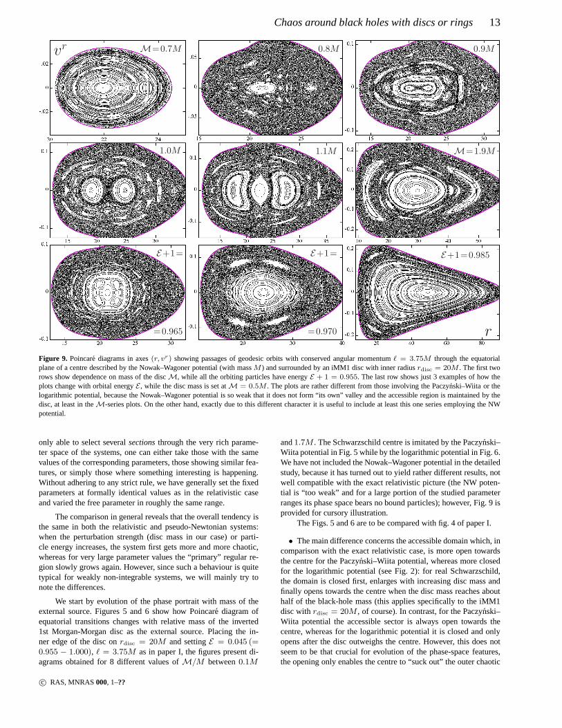
Figure 9. Poincare diagrams in axes(r, vr) showing passages of geodesic orbits with conserved angularmomentumℓ = 3.75M through the equatorialplane of a centre described by the Nowak–Wagoner potential (with massM ) and surrounded by an iMM1 disc with inner radiusrdisc = 20M . The first tworows show dependence on mass of the discM, while all the orbiting particles have energyE + 1 = 0.955. The last row shows just 3 examples of how theplots change with orbital energyE , while the disc mass is set atM = 0.5M . The plots are rather different from those involving the Paczynski–Wiita or thelogarithmic potential, because the Nowak–Wagoner potential is so weak that it does not form “its own” valley and the accessible region is maintained by thedisc, at least in theM-series plots. On the other hand, exactly due to this different character it is useful to include at least this one series employing the NWpotential.

only able to select severalsectionsthrough the very rich parame-ter space of the systems, one can either take those with the samevalues of the corresponding parameters, those showing similar fea-tures, or simply those where something interesting is happening.Without adhering to any strict rule, we have generally set the fixedparameters at formally identical values as in the relativistic caseand varied the free parameter in roughly the same range.

The comparison in general reveals that the overall tendencyisthe same in both the relativistic and pseudo-Newtonian systems:when the perturbation strength (disc mass in our case) or parti-cle energy increases, the system first gets more and more chaotic,whereas for very large parameter values the “primary” regular re-gion slowly grows again. However, since such a behaviour is quitetypical for weakly non-integrable systems, we will mainly try tonote the differences.

We start by evolution of the phase portrait with mass of theexternal source. Figures 5 and 6 show how Poincare diagram ofequatorial transitions changes with relative mass of the inverted1st Morgan-Morgan disc as the external source. Placing the in-ner edge of the disc onrdisc = 20M and settingE = 0.045 (=0.955 − 1.000), ℓ = 3.75M as in paper I, the figures present di-agrams obtained for 8 different values ofM/M between0.1M

and1.7M . The Schwarzschild centre is imitated by the Paczynski–Wiita potential in Fig. 5 while by the logarithmic potentialin Fig. 6.We have not included the Nowak–Wagoner potential in the detailedstudy, because it has turned out to yield rather different results, notwell compatible with the exact relativistic picture (the NWpoten-tial is “too weak” and for a large portion of the studied parameterranges its phase space bears no bound particles); however, Fig. 9 isprovided for cursory illustration.

The Figs. 5 and 6 are to be compared with fig. 4 of paper I.

• The main difference concerns the accessible domain which, incomparison with the exact relativistic case, is more open towardsthe centre for the Paczynski–Wiita potential, whereas more closedfor the logarithmic potential (see Fig. 2): for real Schwarzschild,the domain is closed first, enlarges with increasing disc mass andfinally opens towards the centre when the disc mass reaches abouthalf of the black-hole mass (this applies specifically to theiMM1disc withrdisc = 20M , of course). In contrast, for the Paczynski–Wiita potential the accessible sector is always open towards thecentre, whereas for the logarithmic potential it is closed and onlyopens after the disc outweighs the centre. However, this does notseem to be that crucial for evolution of the phase-space features,the opening only enables the centre to “suck out” the outer chaotic



M=0.003M M=0.12M

M=0.008M M=0.45M

M=0.020M M=0.70M

M=0.055M M=1.10M

r

vr

Figure 10. Poincare(r, vr) diagrams showing passages of geodesics with conserved energy E + 1 = 0.977 and angular momentumℓ = 3.75M throughthe equatorial plane of a centre described by the Paczynski–Wiita potential (with massM ) and surrounded by a Bach–Weyl ring with radiusrring = 20M .Dependence on mass of the ringM is shown, with values given in the plots. Accessible sector is indicated in purple andr axis is in units ofM .



M=0.003M M=0.12M

M=0.008M M=0.30M

M=0.020M M=0.70M

M=0.055M M=1.10M

r

vr

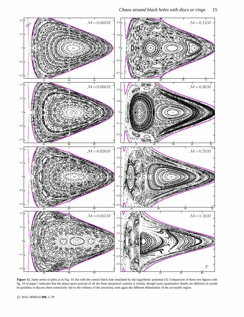
Figure 11.Same series of plots as in Fig. 10, but with the central black hole simulated by the logarithmic potential (3). Comparisonof these two figures withfig. 10 of paper I indicates that the phase-space portrait of all the three dynamical systems is similar, though many quantitative details are different (it wouldbe pointless to discuss them extensively due to the richnessof the structure); note again the different delimitation ofthe accessible region.



E+1=0.915

0.920

0.925

0.930

0.935

0.940

0.945

0.950

0.960

0.965

0.970

E+1=0.985

r

vr

Figure 12.Poincare(r, vr) diagrams showing passages of geodesics with angular momentum ℓ = 3.75M through the equatorial plane again, for the centredescribed by the Paczynski–Wiita potential (with massM ) and surrounded by a Bach–Weyl ring with massM = 0.5M and radiusrring = 20M . Heredependence on energy of the orbitersE is in focus, as indicated by its values given in the plots (we enlarge it by unity again). We are not showing plots obtainedfor E + 1 = 0.910 and less which only contain a tiny accessible region around the ring (the other region between the centre and the ring is not existing yet).

sea. (This makes the open diagrams asymmetric with respect tovr = 0.)• The similarity of all three systems is really striking, withmost

phase-space structures appearing and in the same succession. In thePaczynski–Wiita case, similar features appear for somewhat lowerdisc-mass values (about0.1M÷0.2M “earlier”) than in the rela-tivistic case, while for the logarithmic potential they appear stillabout0.05M÷0.1M earlier than for the PW potential. This may beinterpreted as slightly stronger inclination of the pseudo-Newtoniansystem towards chaos, which is in accord with our preliminaryguess stemming from deeper potential valleys provided by them(see Fig. 3).• More details about the structures: with increasing perturbing

mass, the relativistic geodesic system (see paper I) first developsa 3-fold island within the primary regular region (2:3 resonance,“fish”-shaped orbit in Fig. 17); then (temporarily) a 4-foldone ap-

pears within the chaotic periphery of the accessible region: this isa particularly shaped “symmetrized set” of 1:2 resonances (anal-ogous feature appears “earlier” in the PW case).3 Later the cen-tral regular region gives birth to five islands (4:5 resonance, againidentical in the relativistic and pseudo-Newtonian case),then even7-fold and 9-fold “baby-islands” (6:7 and 8:9 resonances) can bespotted, and finally the region breaks up into two parts symmetricalwith respect tovr = 0 which disappear shortly after the disc massreaches about the black-hole mass. Meanwhile, a central regularsector appears and grows gradually with the disc mass increased

3 Normally, anm:k resonance is associated with ak-fold (k-periodic) is-land. It is not clear whether the 4-fold island represents a tangent or a pitch-fork bifurcation of the 1:2 resonance (cf. also the following commentary ona 1:1-resonance bifurcation).



E+1=0.915

E+1=0.920

0.925

0.930

0.935

0.940

0.945

0.950

0.960

0.965

0.970

E+1=0.985

r

vr

Figure 13.A counterpart of Fig. 12, showing the same series of dependence-on-energy plots for the centre described by the logarithmic potential (3). All theparameters are kept from previous figure, i.e.ℓ = 3.75M , M = 0.5M , rring = 20M , and also the values ofE are chosen equally, as indicated in the plots.In addition, we have kept exactly the same axis ranges, so thetwo figures can be compared easily. Their relativistic counterpart is fig. 12 of paper I.

still more.The Paczynski–Wiita centre with the iMM1 disc also first give birthto the 3-fold island and then to the 5-fold, 7-fold and 9-foldones,corresponding to the same resonances as in the relativisticcase; the4-fold structure only appears in a light-disc stage (along the bor-der of the regular domain). The logarithmic potential yields verysimilar behaviour, with the 4-fold structure not occurringat all.• The breakup of the original central island is a very character-

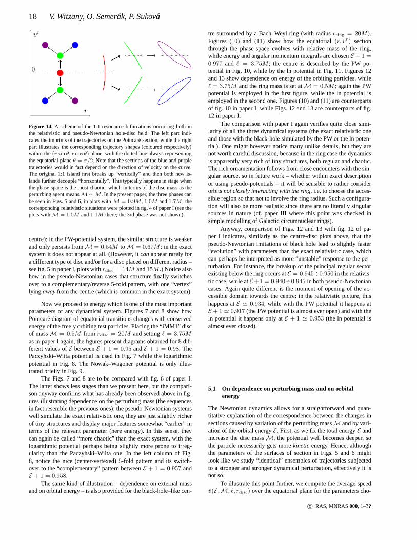
istic feature of the relativistic as well as of the pseudo-Newtoniansystems; in all cases it occurs when the disc massM reaches aboutthat of the central hole (M ). More specifically (Fig. 14): if one takesany pointr, θ, r, θ on the original central orbit (red) and applies thereflectionθ → π − θ and/or velocity-reversalr → −r, θ → −θ,the same central orbit is obtained, just in a different phase. Namely,the central orbit is – up to a phase shift – symmetric with respect toreflection and reversal which are discrete symmetries of theHamil-tonian. However, this symmetry of the whole phase space neednot

be respected byindividual invariant structures. The multiplicationof resonant islands is then a kind of “spontaneous symmetry break-ing”, because as the central orbit shifts to the strongly perturbingdisc edge, it looses stability and bifurcates into two (green) orbitswhich are reflection-symmetric when taken together as a “sym-metrized set” (the reflection operation maps the points of the firsttrajectory on the second one and vice versa). These green trajec-tories later bifurcate even further in the radial direction, into 2+2“reversible-asymmetric” trajectories (blue and purple).The foursmall islands in the Poincare diagrams withM = 1.7M in Figs.5 and 6 thus correspond to a symmetrized set of four distinct 1:1resonances.• Let us point to one specific difference finally: In the log-

potential system, one observes a strong 5-fold structure correspond-ing to a 4:5 resonance inside the central regular region, existingfrom M = 0.33M to M = 0.62M (we mean the one orientedso that one “vertex” island lies on thevr = 0 axis and towards the



r

vr

0

Figure 14. A scheme of the 1:1-resonance bifurcations occurring both inthe relativistic and pseudo-Newtonian hole-disc field. Theleft part indi-cates the imprints of the trajectories on the Poincare section, while the rightpart illustrates the corresponding trajectory shapes (coloured respectively)within the(r sin θ, r cos θ) plane, with the dotted line always representingthe equatorial planeθ = π/2. Note that the sections of the blue and purpletrajectories would in fact depend on the direction of velocity on the curve.The original 1:1 island first breaks up “vertically” and thenboth new is-lands further decouple “horizontally”. This typically happens in stage whenthe phase space is the most chaotic, which in terms of the discmass as theperturbing agent meansM ∼ M . In the present paper, the three phases canbe seen in Figs. 5 and 6, in plots withM = 0.9M , 1.0M and1.7M ; thecorresponding relativistic situations were plotted in fig.4 of paper I (see theplots withM = 1.0M and1.1M there; the 3rd phase was not shown).

centre); in the PW-potential system, the similar structureis weakerand only persists fromM = 0.54M toM = 0.67M ; in the exactsystem it does not appear at all. (However, itcanappear rarely fora different type of disc and/or for a disc placed on differentradius –see fig. 5 in paper I, plots withrdisc = 14M and15M .) Notice alsohow in the pseudo-Newtonian cases that structure finally switchesover to a complementary/reverse 5-fold pattern, with one “vertex”lying awayfrom the centre (whichis common in the exact system).

Now we proceed to energy which is one of the most importantparameters of any dynamical system. Figures 7 and 8 show howPoincare diagram of equatorial transitions changes with conservedenergy of the freely orbiting test particles. Placing the “iMM1” discof massM = 0.5M from rdisc = 20M and settingℓ = 3.75Mas in paper I again, the figures present diagrams obtained for8 dif-ferent values ofE betweenE + 1 = 0.95 andE + 1 = 0.98. ThePaczynski–Wiita potential is used in Fig. 7 while the logarithmicpotential in Fig. 8. The Nowak–Wagoner potential is only illus-trated briefly in Fig. 9.

The Figs. 7 and 8 are to be compared with fig. 6 of paper I.The latter shows less stages than we present here, but the compari-son anyway confirms what has already been observed above in fig-ures illustrating dependence on the perturbing mass (the sequencesin fact resemble the previous ones): the pseudo-Newtonian systemswell simulate the exact relativistic one, they are just slightly richerof tiny structures and display major features somewhat “earlier” interms of the relevant parameter (here energy). In this sense, theycan again be called “more chaotic” than the exact system, with thelogarithmic potential perhaps being slightly more prone toirreg-ularity than the Paczynski–Wiita one. In the left column ofFig.8, notice the nice (center-vertexed) 5-fold pattern and itsswitch-over to the “complementary” pattern betweenE + 1 = 0.957 andE + 1 = 0.958.

The same kind of illustration – dependence on external massand on orbital energy – is also provided for the black-hole–like cen-

tre surrounded by a Bach–Weyl ring (with radiusrring = 20M ).Figures (10) and (11) show how the equatorial(r, vr) sectionthrough the phase-space evolves with relative mass of the ring,while energy and angular momentum integrals are chosenE +1 =0.977 and ℓ = 3.75M ; the centre is described by the PW po-tential in Fig. 10, while by the ln potential in Fig. 11. Figures 12and 13 show dependence on energy of the orbiting particles, whileℓ = 3.75M and the ring mass is set atM = 0.5M ; again the PWpotential is employed in the first figure, while the ln potential isemployed in the second one. Figures (10) and (11) are counterpartsof fig. 10 in paper I, while Figs. 12 and 13 are counterparts of fig.12 in paper I.

The comparison with paper I again verifies quite close simi-larity of all the three dynamical systems (the exact relativistic oneand those with the black-hole simulated by the PW or the ln poten-tial). One might however notice many unlike details, but they arenot worth careful discussion, because in the ring case the dynamicsis apparently very rich of tiny structures, both regular andchaotic.The rich ornamentation follows from close encounters with the sin-gular source, so in future work – whether within exact descriptionor using pseudo-potentials – it will be sensible to rather considerorbitsnot closely interacting with the ring, i.e. to choose the acces-sible region so that not to involve the ring radius. Such a configura-tion will also be more realistic since there are no literallysingularsources in nature (cf. paper III where this point was checkedinsimple modelling of Galactic circumnuclear rings).

Anyway, comparison of Figs. 12 and 13 with fig. 12 of pa-per I indicates, similarly as the centre-disc plots above, that thepseudo-Newtonian imitations of black hole lead to slightlyfaster“evolution” with parameters than the exact relativistic case, whichcan perhaps be interpreted as more “unstable” response to the per-turbation. For instance, the breakup of the principal regular sectorexisting below the ring occurs atE = 0.945÷0.950 in the relativis-tic case, while atE+1 = 0.940÷0.945 in both pseudo-Newtoniancases. Again quite different is the moment of opening of the ac-cessible domain towards the centre: in the relativistic picture, thishappens atE ≃ 0.934, while with the PW potential it happens atE +1 ≃ 0.917 (the PW potential is almost ever open) and with theln potential it happens only atE + 1 ≃ 0.953 (the ln potential isalmost ever closed).

5.1 On dependence on perturbing mass and on orbitalenergy

The Newtonian dynamics allows for a straightforward and quan-titative explanation of the correspondence between the changes insections caused by variation of the perturbing massM and by vari-ation of the orbital energyE . First, as we fix the total energyE andincrease the disc massM, the potential well becomes deeper, sothe particle necessarily gets morekineticenergy. Hence, althoughthe parameters of the surfaces of section in Figs. 5 and 6 mightlook like we study “identical” ensembles of trajectories subjectedto a stronger and stronger dynamical perturbation, effectively it isnot so.

To illustrate this point further, we compute the average speedv(E ,M, ℓ, rdisc) over the equatorial plane for the parameters cho-



0.2 0.4 0.6 0.8

0.948 0.950 0.952 0.954 0.956

0.08

0.09

0.10

0.11

0.12

0.13

✻

v

✲

M/M

✲E+1

Figure 15.Average speed (35) with which the orbits (havingℓ = 3.75M )intersect the equatorial plane of the system of a black hole surrounded bythe iMM1 disc with inner radiusrdisc = 20M . The dependence ofv onthe relative disc massM/M is plotted forE + 1 = 0.955 (these curvesare given in× crosses; top axis applies); the dependence ofv on the con-served energyE is plotted for the disc massM = 0.5M (these curves aregiven in solid diamonds; bottom axis applies). The top couple of curves hasbeen obtained for the Paczynski–Wiita potential, while the bottom (fastergrowing) couple for the logarithmic potential. In both cases, v grows al-most monotonously withM as well as withE , having a single “dip” whichis associated with the phase when the accessible region reaches above thedisc edge.

sen in Figs. 5–8,4

v(E ,M, ℓ, rdisc) =

∫√

2 [E − Veff(θ=π/2)] 2πr dr∫

2πr dr, (35)

and plot the dependence of the result onM andE for the PW andln potential in Fig. 15. (Integration is performed over the accessibleregion; in cases where the the latter was not closed in the directiontoward the centre, we have taken the lowest reachabler to be5M .)In the ranges0 . M . 0.8M and0.945 . E+ 1 . 0.965 (ofwhich part is shown in the figure), and for both central potentials,the growth ofv with eitherM or E is very similar. The comparisonof plots shown in Fig. 15 thus suggests the following interpretation:the phase-space structure stays roughly the same for a moderatedisc-mass perturbation, with the growing disc mass mostly induc-ing a shift of the orbits to higher kinetic energies. This aspect issurely present in the relativistic case studied in papers I–III as well,but would require a more subtle argument.

5.2 Remark on the Bach–Weyl ring

The Bach–Weyl ring is actually an interesting source. Its poten-tial (29) is everywhere attractive, namely its field intensity (minusgradient of the potential) points toward the ring from all local lat-itudinal directions. In the Newtonian picture it thus represents an“ordinary” ring source. In relativity the potential remains valid, butthe metric involvestwo functions, the second being given by a lineintegral of the potential gradient. In the BW-ring case, both func-tions are given by elliptic integrals and, as expected, bothdivergeat the very ring. The two divergences however combine to sucha

4 The “average speed” is certainly an ambiguous concept. We choose herea definition which is simple and natural.

deformation of geometry in the ring’s vicinity that the realphysicaldistance (proper distance) to the ring comes out finite from out-side (when the ring is approached from bigger radii), whereas infi-nite from inside (when the ring is approached from smaller radii).When free motion is plotted in coordinates, the particles thus ap-pear repelled/attracted by the ring in the directions from whichthe ring is physically nearby/far away, i.e., they seem to bere-pelled towards larger radii, whereas attracted from smaller radii.The effect is strongest in the equatorial region. We noticedit andinterpreted in Semerak et al. (1999), and later this was repeated byD’Afonseca et al. (2005).

Since the above feature is “felt” up to several tenths of ringmass in the Weyl or Schwarzschild coordinates (in geometrizedunits), it might be somehow reflected in orbital statistics.How-ever, the effect is much better seen in themeridionalplane (thanin the equatorial one): the coordinate tracks of free particles, whenapproaching the ring from any latitudinal direction, are driven to-wards its inner side and hit it just along the equatorial plane. Inspec-tion of the ring’s neighbourhood in Poincare plots does notseem toindicate stronger anisotropy in the relativistic case. Onecan onlyobserve slight differences in evolution of the main regularregioncentered just above the ring: for small ring mass, it is central sym-metric in all three descriptions, but when the mass reaches severalpercent ofM , it “elongates” along thevr = 0 direction and fi-nally two new islands establish on its opposite radial sides, createdby orbits circling around (“through”) the ring. This process startssomewhat beforeM = 0.02M in the relativistic system as well asin the system using the ln potential, while in the PW-potential caseit starts only beforeM = 0.03M . The only qualitative differencebetween the relativistic and the pseudo-Newtonian systemsis thatin the latter case, for large ring masses (fromM = 0.8M for the lnpotential, while fromM = 0.9M for the PW potential) a new pairof regular regions appear, again symmetrically with respect to theprincipal island, but now both lieabovethe ring radius. See mainlythe last plot (M = 1.1M ) of the ln-potential Fig. 11, where thesetwo islands already dominate the section. It would be interestingto check whether the lack of this regular couple in the relativisticsystem has connection with the ring’s outward repulsion.

However, it should be noted that the Poincare-surface analysisis best suited for the demonstration of long-term effects inthe mo-tion of eternally orbiting particles, whereas the above mentionedfeature mainly affects trajectories soon to be captured by the ring.Thus, the Poincare section will typically bear one or two pointsfrom such trajectories and their dynamical behaviour will be hardlydiscernible for most part. The only effect one could hope to observein the surfaces of section is a deformation of invariant structures –of which we find no persuasive evidence.

5.3 Resonance and chaos in orbit shapes

Poincare surfaces of section represent a basic tool for assessing theoverall structure of the possible test-particle motion, but one shouldkeep in mind that they are really justsectionsthrough phase space,flattening out most of the information about individual trajectories.When comparing different systems, like the relativistic one and itspseudo-Newtonian counter-parts we are interested in here,one nat-urally first checks the Poincare diagrams for analogies andvari-ances, but in fact any statements concerning the occurrenceof cer-tain structures in Poincare sections has to be taken with caution,because a particular sequence of recorded points (e.g. equatorialtransitions) does not in general unveil a trajectory uniquely.

In order to get an idea of what trajectory shapes such struc-



10 15 20 10 15 20 10 15 20

10 15 20 10 15 20 10 15 20

10 15 10 15 10 15 10 15 10 15

10 15 10 15 10 15 10 15 10 15 10 15 13

2

-2

2

-2

2

0

-2

4

-4

4

0

-4

✻r cos θ✲

r sin θ

Figure 17. A counterpart of Fig. 16, showing the shapes within ther sin θ, r cos θ plane of the trajectories whose equatorial transitions have been recordedthere (in ther, vr axes). The orbits are plotted up to some 200 periods and are coloured to be easily identifiable in Fig. 16. From top left to right and bottom,the profile starts from the central orbit of the 3-fold islandand proceeds toward the centre of the Fig.-16 surface of section. All the plots have exactly thesame scale, though the coordinate ranges (indicated along the axes in units ofM ) are adjusted to capture the orbits effectively. Orbits from “more interesting”regions are purple, one chaotic orbit is green.

tures may represent and to illustrate what the statements about thefrequency ratios mean for the actual trajectories, we select one ofthe sections obtained within the series capturing the dependenceon iMM1-disc mass, namely theM = 0.35M section of Fig.6 (where the black hole was simulated by the logarithmic poten-tial). This case represents the weakest perturbation for which sep-aratrix chaos already appears near the 3-fold island; the diagram

is repeated in Fig. 16 with a selection of orbits plotted in colours.The motion in theφ direction is dynamically unimportant (boundby conserved integralℓ) in the axially symmetric case, so we sup-press this dimension and illustrate the orbital shapes within theWeyl (ρ, z) meridional plane. The results are grouped in Fig. 17,marked by the same colours as their equatorial sections in Fig. 16.

There are two distinct structures in Fig. 16, the 3-fold and the



r

vr

Figure 16. The Poincare diagramM = 0.35M from Fig. 6 revisitedwith the aim to illustrate what kind of orbits its main structures represent.About 7400 transitions for each orbit has been recorded. Theorbits areshown in colour to ensure their easy identification against Fig. 17 wherethe meridional-plane shapes of their 200 periods are plotted.

5-fold island; the ratio of the radial to vertical frequencies is 2:3for the former and 4:5 for the latter. The shapes of the trajectoriesreveal less thick resonances hidden in both the central and 3-fold is-land, but for most of them only a longer evolution track couldcon-firm whether it is actually a resonance or a near-periodic orbit only.However, one can notice a certain deformation due to the proximityof a resonance in Fig. 17: the fish-like shape of the 2:3 trajectorycorresponding to the 3-fold island is reflected in a significant partof the neighbouring non-resonant phase space, which might per-haps lead to observable signs in an ensemble of particles orbitingnear the black hole. Besides obvious structures, one also notices,when recording data for Fig. 16, that the computation of the singlepurple orbit lying within the (blue) regular single-periodic regiontakes much longer time than that of the other orbits around. Thistypically indicates that one is close to a resonance, which is con-firmed in Fig. 17. Let us also point out to the rightmost orbit inthe last-but-one row and to the middle one in the last row (bothare purple): they are very similar, both lying just between a“box”regime and a resonant regime of the regular region, and analogousto a rotation of a pendulum very close to libration; the spatial cor-ridors more densely filled by the orbit in Fig. 16 then correspond tothe pendulum near-stopping at the unstable top equilibrium(beforefalling back to rotation) which stands for an unstable counter-partof the stable periodic orbit at the resonance core.

As seen in the second row of Fig. 17, the time span corre-sponding to some 200 equatorial-plane intersections is notenoughto discern between the regular trajectory (red) and the verycloseseparatrix chaos (green). On the other hand, the respectivesurfaceof section in Fig. 16 allows to discern order and chaos unambigu-ously at the toll of 7400 equatorial intersections. To better under-stand the computational/observational times required fora cleardistinction between the regular and weakly chaotic orbit, we em-ploy a time-series recurrence analysis in the following section.

5.4 Recurrence analysis

It is appropriate to support the Poincare-section observations bysome other independent method. Like in paper II, we turn to tworecurrence methods here, one based on statistics over directions inwhich the orbits traverse a pre-selected mesh of phase-space cells,

the other built on recurrences themselves to the neighbourhoods ofphase-space points.

Kaplan & Glass (1992) suggested to monitor the evolution ofa tangent to the trajectory in small subsets of phase space whichare crossed recurrently. For this purpose, the phase space is “recon-structed” from a given data seriesx(τ ) (either computed or mea-sured) by adding the latter’s replicas delayed by some shift∆τ andits multiples. The method was designed to distinguish between de-terministic and random systems, but we saw in paper II that itisquite sensitive to weak irregularities and thus very well able to alsorecognize how chaotic the (deterministic) system is. Without goinginto details (see paper II for description of how we use the methodfor our system), let us only recall main points:

• First the dimensiond is chosen of the phase space to be re-constructed, plus the delay∆τ and the size of boxes into which thephase space is divided.• Average tangents of a trajectory within a given (jth) box are

summed (vector addition) for a large number of recurrent transitsand the length of the result is suitably normalized; the result is de-noted asVj(∆τ ).• The resulting norm is averaged then over all boxes which were

crossed exactlyn-times.• The result depends onn, on d, on∆τ and on the lattice-box

size. (The choice of these parameters in turn depends on how longdata series one deals with.) Withn it decreases roughly asn−1/2

for random data, whereas more slowly for a deterministic system(in a theoretical limit of an infinitely long series and infinitesimallyfine grain, it even remains 1 for the deterministic case). Thedepen-dence on∆τ is specifically studied on the deviation of the resultfrom the value obtained for random walk, computed for each boxand then averaged over all occupied boxes,

Λ = Λ(∆τ ) :=

⟨

[Vj(∆τ )]2 − (Rdnj)2

1− (Rdnj)2

⟩

(Rdnj

is the average displacement per step for random walk oflengthnj in d dimensions). In a theoretical limit,Λ = 0 for arandom walk, whereasΛ = 1 for a deterministic system; in prac-tice, Λ falls off roughly as autocorrelation function for a randomseries, while more slowly for a deterministic one.

We have subjected to the Kaplan–Glass test two orbits fromFigs. 16 and 17, namely the outmost of the red-colour (3-fold) reg-ular ones and the nearby green-colour chaotic one which has arisedfrom a separatrix breakup. The autocorrelation corresponding tothe dependence of the “directional-vectors average”Λ on time de-lay∆τ clearly confirms the different character of the orbits. Let usspecify that we started the analysis from reconstructing the phasespace as three-dimensional and dividing it in253=15625 boxes;average number of transitions through one box (among those whichwere crossed at least once) has been around 50.

The second method rests on the statistics of recurrences to pre-scribed neighbourhoods of phase-space points (either of the “orig-inal” phase space, or the reconstructed one). Marwan et al. (2007)elaborated various useful outcomes of such a statistics andcodifiedtheir computation in theRECURRENCE PLOTSsoftware; we alreadyapplied it, in paper II, to the exact relativistic system.

The main object of the analysis is the symmetric recurrencematrix

Ri,j(ǫ) = Θ (ǫ− ‖Xi −Xj‖) , i, j = 1, ..., N , (36)

whereXi = X(τi) denoteN successive points of a given phasetrajectory,ǫ is the radius of a chosen neighbourhood (called thresh-



0.2

0.4

0.6

0.8

1.0

0.2

0.4

0.6

0.8

1.0

✻Λ

✲∆τ

(∆τ values given in thousands of M)

regular chaotic

Figure 18.Two “neighbouring” orbits from Fig. 16 (and 17), namely the outmost of the red-colour (3-fold) regular ones (left plot) and the green-colour chaoticone (right plot), are clearly distinguished by the Kaplan–Glass “average directional vectors” recurrence method. Themeaning of theΛ(∆τ) dependence isexplained in the main text. Recall that both orbits represent motion of free particles withE + 1 = 0.955, ℓ = 3.75M in the field of a centre described by thelogarithmic potential (massM ) and surrounded by the iMM1 disc with massM = 0.35M and inner radiusrdisc = 20M . The orbits have been followed forabout500 000M of proper time (some 5000 periods); the top row shows the dependenceΛ(∆τ) from ∆τ = 0 up to∆τ = 100 000M , while three selectedintervals of∆τ are added in more detail in the bottom row (the∆τ -axis labels are in thousands ofM everywhere).

old),Θ is the Heaviside step function and‖ · ‖ denotes the chosennorm (we use a simple Euclidean norm, but other can be consid-ered, without significantly affecting the results). The matrix con-tains only units (meaning thatj-th point is close to thei-th and rep-resented by black dots) and zeros (blank positions which mean theopposite). For regular systems, the recurrences arrange indistinctstructures, in particular in long parallel diagonal lines and checker-board structures, whereas for random systems they are scatteredwithout order; the chaotic systems provide something in between.A number of useful “quantifiers” can then be extracted from the re-currence data, as explained in Marwan et al. (2007) and also brieflyreviewed in our paper II. The simplest ones follow from the lengthsof the diagonal and vertical/horizontal lines which have occurred inthe recurrence matrix.

The recurrence pattern clearly depends on the time step∆τwith which the trajectory is sampled and on the “target” radius ǫ.Besides that, the matrix often contains false recurrence records thatshould be discarded from statistics. For example, ifǫ is too largeand the time step too small, several successive points of thetrajec-tory of courselie within theǫ-neighbourhood of each other, but donot represent true recurrences. Due to the same reason, the real re-currences may then involve more than one point, even if the orbitcomes across its certain previous part in quite a divergent manner.To overcome such false signals, several further “thresholds” are in-

troduced and adjusted, mainly the minimal lengths of relevant di-agonal and vertical lines,lmin andvmin.

The choice of the recurrence thresholdǫ should also take intoaccount the physical extent of the orbit and its variance. However,we overcome this ambiguity by rescaling the time series in such away that each variable has zero mean and unit variance. This alsoassures that motion in all coordinate directions have equalweightin the analysis, irrespective of the actual ranges spanned by the tra-jectory.

For the relativistic–pseudo-Newtonian comparison using therecurrence-matrix analysis, we choose fig. 12 of paper II. There,several “quantifiers” were computed for 470 geodesics havingspecific energyE = 0.9532 and specific angular momentumℓ = 3.75M , sent tangentially (withur = 0) from radii betweenr = 5M andr = 24M (with step0.04M ) from the equatorialplane of the system of a black hole (M ) and the iMM1 disc withM = 0.5M andrdisc = 18M . The orbits were followed for about250 000M of proper time with “sampling period”∆τ = 45M ,the minimal length of diagonal/vertical lines has been set at 90Mand the radius of the recurrence neighbourhood (the threshold) atǫ = 1.25. Two of the quantifiers – the most simple one calledDIV ,given by reciprocal of the longest recurrence-matrix diagonal, anda much more “sophisticated” one read off from the slope of thehistogram of diagonals (and providing an estimate of the maximal



relativistic pseudo-Newtonian(ln potential)

ur ur

r/M r/M

DIV DIV

DET DET

r/M r/M

Figure 19. Examples of the recurrence-plot results, obtained for freemotion with E(+1) = 0.9532 and ℓ = 3.75M in the black-hole–disc field withM = 0.5M andrdisc = 18M . Exact relativistic system is represented in theleft column, while pseudo-Newtonian system employing the logarithmicpotential is in theright column. The top row shows Poincare diagrams coloured according tothe value ofDIV whoseur = 0/vr = 0 radial profile is alsoplotted in the middle row (going from blue to red, the value ofDIV increases, which corresponds to increasing irregularity); the bottom row shows the sameprofile for another simple quantifierDET , given by ratio of the points which form a diagonal line longer than a certain minimum. The horizontal axes (r inunits ofM ) are common for all rows and the vertical axes are common for both columns. One more remark: notice that in the left Poincare section the orangeand red orbits are rather separated, whereas in the right onethey are mixed within the chaotic sea. This is because the left section is actually divided into a“sticky” interior region harbouring weaker chaos and only slowly diffusing particles, and the outer chaotic sea with strong chaos. In the right section, the outerlayer is mixed orange-red, with its less chaotic orange trajectories perhaps corresponding to motion “sticked”, for a short time, to the three small islands on theoutskirts. ForM ≈ 0.65M the green layer of very weak chaos gets connected with the outskirts, thus yielding a picture rather similar to the relativistic case.



Lyapunov exponent), were particularly illustrated by colouring thecomputed orbits according to their values in the Poincare diagram.Two main observations were made: i) all the quantifiers proved sen-sitive to even tiny phase-space features, and ii) the computationallyeasyDIV quantifier proved equally efficient as the more sophisti-cated one.

The above recurrence analysis was performed in a 6D phasespace (r, θ, φ and the respective velocities), while, for the presentcomparison, we have repeated it, for the same set of geodesics,in the (r sin θ, r cos θ) plane plus the respective velocity dimen-sions only. Elimination ofφ from the analysis has some interestingaspects, even though it is a Killing-symmetry coordinate. For in-stance, note that in the full 3D configuration space there arevirtu-ally no true recurrences, since even the most regular central orbit isquasi-periodic inφ. Within the meridional plane, on the other hand,the resonance cores produce true recurrences (see section 5.3).

Let us add that theφ coordinate can be viewed as a kind of“dynamical memory”, because

∆φ =

∫

∆t

ℓ dt

r2 sin2 θ(37)

(a relativistic formula only contains proper timeτ instead oft).Hence, the inclusion ofφ actually adds non-trivial information, sothe change resulting from its elimination might indicate the robust-ness of various recurrence indicators.

The parameters we have used for the re-analysis of fig. 12 ofpaper II arelmin = 3 andvmin = 3 for the minimal diagonal andvertical, the Theiler windoww = 3 and the neighbourhood radiusǫ = 0.8 (with Euclidean metric used for the distance). The trajec-tories for the recurrence matrix were then recorded at a timestep∆τ = 45M for a total time of about250 000M like in paper II.As can be seen in Fig. 19, theDIV indicator is not changed bythe 3D→2D projection at all, whereas theDET quantifier turnedout to be less robust in this respect. In particular, theDET quanti-fier seems to wrongly indicate that a large part of the centralislandis “less deterministic” than the surrounding chaos. To understandthis point, let us recall that theDET indicator is defined as theratio of the number of diagonal lines longer thanlmin to the num-ber of recurrence points. We checked that the orbits in the centralisland show a large number of recurrence points but not alwaysgrouped into longer diagonal lines. The performed normalizationwith respect to the total number of recurrence points thus has anundesirable effect in this case.

Now to the comparison: we take an analogous pseudo-Newtonian situation, namely the gravitational system with“thesame” parameters and with the central black hole simulated by thelogarithmic potential (we do not employ the Paczynski–Wiita one,because that yields rather open accessible region, which makes thechaotic sea efficiently drained away to the centre), and subject itto the same recurrence-matrix analysis as performed in fig. 12 ofpaper II; the results are given in Fig. 19. Clearly the phase-spacestructure is rich for the given parameters and also rather differentfrom its paper-II counter-part. (As already stressed above, the rela-tivistic and pseudo-Newtonian systems are qualitatively similar, butthe similar phase-space pictures are somewhat shifted withrespectto each other in the parameter space.) The question is whether thecorresponding recurrence patterns are still not alike, in spite of thisfirst-sight difference.

In Fig. 19, the left column is relativistic and the right column ispseudo-Newtonian (with the logarithmic potential), both plotted inthe same scale. Both Poincare sections are coloured by the longest-diagonal reciprocalDIV , the latter’s zero-velocity radial profile

being also plotted below, and the last row shows another simplequantifierDET , given by ratio of the points which form a diago-nal line longer than a certain value within all the recurrence points.Although the surfaces of section reveal rather different structures,we do not see any big overall divergence in the recurrence charac-teristics.

CONCLUDING REMARKS

We have considered Newtonian dynamical systems describingthe massive-test-particle motion in a gravitational field of aSchwarzschild-like centre simulated by a suitable potential andsurrounded symmetrically by a gravitating thin disc or ring. Try-ing to learn how they differ from the corresponding relativisticsystem, namely the time-like geodesic dynamics in the field of aSchwarzschild black hole surrounded by “the same” disc or ring(described by the same Newtonian potential), we plotted Poincarediagrams of equatorial transitions for a number of similar situa-tions (same coordinate position and relative mass of the disc orring, same values of the particles’ conserved energy and angularmomentum) and found similar tendencies, typical for weaklynon-integrable systems. The picture revealed by the surfaces ofsec-tion was also confirmed by two recurrence methods, one resting onstatistics over directions in which the orbits transit recurrently theboxes of a pre-selected phase-space mesh, and the other analysingthe recurrences themselves to some prescribed neighbourhood ofphase-space points. We have been using adifferent code than inprevious papers of this series, so the present results also supportrobustness of the observations made.

A careful conclusion would be that the pseudo-Newtonian ap-proach can reproduce the long-term dynamics of our relativisticsystem reasonably, though there appear various quantitative differ-ences. However, this conclusion strongly depends on the potentialused to mimic the black-hole centre: the Paczynski–Wiita and thelogarithmic potentials provide results very similar to therelativis-tic treatment, while the Nowak–Wagoner potential offers quite adifferent picture; some other potentials are not suitable for thesepurposes at all (although they may be efficient in another context).Yet even the Paczynski–Wiita and the logarithmic potentials dif-fer considerably (from the relativistic system as well as from eachother) in the phase-space accessible region they determine– thePW potential is too open, whereas the ln potential is too closedin direction toward the centre, which mainly affects how effec-tively the centre “sucks out” the chaotic orbits; nevertheless, thisdoes not seem to influence much the behaviour of regular structuresunder parameter change. Generally, the pseudo-systems (involvingthe PW and mainly the ln potential) can be labelled slightly moreunstable than the exact relativistic system, since their phase-spacestructures evolve somewhat faster with parameters.

As mentioned in preceding papers, there are several possi-ble directions of further study. One can certainly subject the dy-namical system – either the relativistic or the (pseudo-)Newtonianone – to still other methods (than already employed there), e.g.the Melnikov-integral calculation or the basin-boundary analysis,or to a more detailed study of its particularly “interesting” orbits(mainly the periodic ones). However, most important astrophysi-cally is to make our setting more realistic and to try to confront itwith what is going on in real celestial systems. The simplestissue,at least within the static and axially symmetric situation,would beto add another gravitating components like central star cluster, ajet or a halo. Second, we plan to consider non-singular (i.e.3D)



sources instead of the infinitesimally thin ones. This is especiallyimportant in systems where the orbits can reach very close tothesources, mainly in the relativistic description when the rings as wellas edges of the thin discs usually represent a curvature singularityand (thus) the space-time is unnaturally deformed in their vicinity.In particular, one would be interested in how reasonably – asfar asthe long-term dynamics is concerned – the singular (Bach–Weyl)ring can approximate a toroidal source; this could be studied on asequence of toroids gradually thinning to a ring.

Once obtaining a sufficiently realistic description, it is desir-able to look for consequences for observational phenomena.Forinstance, the ensembles of initial conditions studied in the surfacesof section can be understood asactual collisionless ensembles ofparticles orbiting a black hole. The increased “suck-in” ofthe en-semble under perturbation then imply an enhanced accretionrate,while the resonances, on the other hand, correspond to particularlybehaving oscillation modes.

And then there aredifficult aspects of “realisticity”: incorpo-rating (adequately) rotation of the gravitating bodies (which bringsdragging effects into the relativistic systems) and possibly also backreaction resulting from the non-test character of the orbiter.

ACKNOWLEDGEMENTS

Access to computing and storage facilities owned by partiesand projects contributing to the Czech National Grid Infrastruc-ture MetaCentrum, provided under the programme “Projects ofLarge Infrastructure for Research, Development, and Innovations”(LM2010005), is greatly appreciated. The plots were producedwith the help of the GNUPLOTutility, C. Louvrier’s PNGSLIM pro-gram and D. Krause’sBMPP program. We are grateful for supportfrom grants GAUK-2000314 (V.W.); GACR-14-10625S (O.S.);DEC-2012/05/E/ST9/03914 (P.S.). O.S. also thanks M. Crosta forkind hospitality at the Osservatorio Astrofisico di Torino.

REFERENCES

Artemova I. V., Bjornsson G., Novikov I. D., 1996, ApJ, 461,565Blanes S., Moan P. C., 2002, J. Comp. Appl. Math., 142, 313Chakrabarti S. K., Mondal S., 2006, MNRAS, 369, 976Crispino L. C. B., da Cruz Filho J. L. C., Letelier P. S., 2011,Phys.Lett. B, 697, 506

D’Afonseca L. A., Letelier P. S., Oliveira S. R., 2005, Class.Quantum Grav., 22, 3803

Ghosh S., Sarkar T., Bhadra A., 2014, MNRAS, 445, 4463Gueron E., Letelier P. S., 2001, Astron. Astrophys., 368, 716Hairer E., Wanner G., Lubich C., 2006, Geometric NumericalIntegration. Structure-Preserving Algorithms for Ordinary Dif-ferential Equations, Springer Ser. in Comp. Math. 31, Springer,Berlin Heidelberg

Ivanov R. I., Prodanov E. M., 2005, Phys. Lett. B, 611, 34Kaplan D. T., Glass L., 1992, Phys. Rev. Lett., 68, 427Karas V., Abramowicz M. A., 2015, in Proc. RAGtime 14–16:Workshop on black holes and neutron stars, eds. S. Hledık,Z. Stuchlık (Silesian Univ. in Opava, Opava 2015), to appear(arXiv:1412.6832 [astro-ph.HE])

Marwan N., Romano M. C., Thiel M., Kurths J., 2007, Phys. Re-ports, 438, 237

Nowak M. A., Wagoner R. V., 1991, ApJ, 378, 656Paczynski B., Wiita P. J., 1980, A&A, 88, 23

Selaru D., Mioc V., Cucu-Dumitrescu C., Ghenescu M., 2005,As-tron. Nachr., 326, 356

Semerak O., 2015, ApJ, 800, 77Semerak O., Karas V., 1999, A&A, 343, 325Semerak O., Sukova P., 2010, MNRAS, 404, 545 (paper I)Semerak O., Sukova P., 2012, MNRAS, 425, 2455 (paper II)Semerak O.,Zacek M., Zellerin T., 1999, MNRAS, 308, 705Seyrich J., Lukes-Gerakopoulos G., 2012, Phys. Rev. D, 86,124013

Steklain A. F., Letelier P. S., 2006, Phys. Lett. A, 352, 398Steklain A. F., Letelier P. S., 2009, Phys. Lett. A, 373, 188Stoffer D., 1995, Computing, 55, 1Stuchlık Z., Kovar J., 2008, Int. J. Mod. Phys. D, 17, 2089Sukova P., Semerak O., 2013, MNRAS, 436, 978 (paper III)Tejeda E., Rosswog S., 2013, MNRAS, 433, 1930Tejeda E., Rosswog S., 2014, Generalized Newtonian descriptionof particle motion in spherically symmetric spacetimes, submit-ted (arXiv:1402.1171 [gr-qc])

Vokrouhlicky D., Karas V., 1998, MNRAS, 298, 53Wang Y., Wu X., 2011, Commun. Theor. Phys., 56, 1045Wang Y., Wu X., 2012, Chin. Phys. B, 21, 050504Wang Y., Wu X., Sun W., 2013, Commun. Theor. Phys., 60, 433Wegg C., 2012, ApJ, 749, 183Yoshida H., 1990, Phys. Lett. A, 150, 262Zacek M., Semerak O., 2002, Czechosl. J. Phys., 52, 19


http://arxiv.org/abs/1412.6832

http://arxiv.org/abs/1402.1171

Free motion around black holes with discs or rings ... · Free motion around black holes with discs...

Documents

Transcript of Free motion around black holes with discs or rings ... · Free motion around black holes with discs...