Francesco Zirillik OTIC
72
AD-A253 433 , it 1, tj Il 1i I 11 f NUMERICAL OPTIMIZATION Final Technical Report - by Francesco Zirillik O"TIC ~JUL 49 I December 1992 United States Army EUROPEAN RESEARCH OFFICE OF THE U.S. ARMY London England CONTRACT NUMBER DAA 45 - 85 - C - 0028 UniversitA di Roma "La Sapienza", Italy Appvoved for Public Release: distribution unlimited 22 02:5 92- 19828 92 7 2 1111111I'l I I'l
Transcript of Francesco Zirillik OTIC

AD-A253 433, it 1, tj Il 1i I 11 f
NUMERICAL OPTIMIZATION
Final Technical Report
- by
Francesco Zirillik
O"TIC~JUL 49 IDecember 1992
United States Army
EUROPEAN RESEARCH OFFICE OF THE U.S. ARMY
London England
CONTRACT NUMBER DAA 45 -85 - C - 0028
UniversitA di Roma "La Sapienza", Italy
Appvoved for Public Release: distribution unlimited
22 02:5 92- 1982892 7 2 1111111I'l I I'll]l
Abstract
In the framework of the proposed "continuous approach" to constrai-
ned optimization problems, we describe two new solution methods which re-
sulted from the research. The first is a continuous "inexact" method for sol-
ving systems of nonlinear equations and complementarity problems (along
the lines of the DAFNE Method), and the second is a continuous method
for solving the linear programming problems (along the lines of Karmarkar's
method) which is shown to be quadratically convergent.
Some numerical experience on a number of test problems is reported.
Keywords
Numerical Optimization
Constrained Optimization
Systems of nonlinear equations
Complementarity ProblemsLinear Programming
Karmarkar's method
Accessionl For
NTIS CTA&IDTIU TA3 0Unj,, I-j r,',n ee d 0
Just f lent l o
Distr-ibution/
Aval abilitY CodesAvaii and/or
- 29 Dist Spoo al
jv'..

NUMERICAL OPTIMIZATION
Final Technical Report
by
Francesco Zirilli
December 1992
United States Army
EUROPEAN RESEARCH OFFICE OF THE U.S. ARMY
London England
CONTRACT NUMBER DAJA 45 - 85 - C - 0028
UniversitA di Roma "La Sapienza", Italy
Approved for Public Release: distribution unlimited
SI I I I I I I I I I 1
-2-
Table of Content
1 - Introduction Pag. 3
2- Objective of the research " 33 - Results of the research " 3
3.1. The first paper " 4
3.2. The second paper " 5
4- Conclusions " 75- References " 9
List of appendices
Appendix 1
F. Aluffi-Pentini, V. Parisi, F. Zirilli
An Inexact Continuous Method for the Solution of Large Systems of Equa-
tions and Complementarity Problems,
Rend. di Mat., Sez. VII, vol. 9, p. 521-543 (1989).
Appendix 2
S. Herzel, M.L. Recchioni, F. Zirilli
A Quadratically Convergent Method for linear Programming,
Lin. Alg. and its Applications, 155, 255-289 (1981).

-3-
1 . Introduction
This is the final report on the work performed from September 1986
to December 1991, under contract n. DAJA 45-86-C-0028 awarded to the
University of Rome "La Sapienza" on the research project "Numerical Opti-
mization", by the principal investigator Francesco Zirilli and his co-workers.
The objective of the research is described in par. 2, the results of the
research are described in par. 3, and some conclusions are in par. 4.
2. Objective of the research
The subject of the research was the field of those problems in con-
strained optimization which, starting from the linear programming problem,
can be formulated, with growing degree of generalization, first as linear
complementarity problems and second as nonlinear complementarity pro-
blems.
The objective of the research was to attack the above problems bymeans of the so-called "continuous approach" to optimization (as opposed to
the so-called "pivotal" methods, such as the simplex method for linear pro-gramming), with special consideration for the interesting cases of non-con-vex or ill-conditioned problems, and problems with a very large number of
variables; and in particular the objective was to investigate the possibility of
applying to the above problems, suitably transformed into no-ilinear equa-
tion problems, the methods developed by the principal investigator and his
co-workers for solving nonlinear equations and global optimization pro-blems, based on the numerical integration of suitable ordinary or stochastic
differential equations (refs. [1] to [4]).
3. Results of the research
During the development of the research the complementarity pro-
4
blems proved to be much more difficult than it had been anticipated and it
became clear that the original plans where somehow too ambitious.
The final outcome of the research, if judged against the original
plans, is therefore admittedly less satisfactory than it was originally hoped;
nevertheless a number of interesting results have been obtained, so that we
feel that the research is still to be considered at least partially successful.
The main results of the research are contained in the two papers
numbered [5] and [6] in the list of references, which are described in the fol-
lowing paragraphs 3.1 and 3.2, and enclosed as Appendix 1 and Appendix 2.
Report on some work performed in other directions along the lines of
the original research plan, together with some related results of auxiliary
and preliminary nature, were described in the Periodic Technical Reports;
see also the papers numbered [8] and [9] in the list of references.
The research has also stimulated scientific contacts with several ita-
lian and foreign scholars.
The above results have been disseminated by means of the aforemen-
tioned papers on high-standard academic journals, and seminars at Accade-
mia dei Lincei, Rome (ref. [7], which originated paper [8]), at two meetings
of CECAM, Centre Europ~en de Calcul Atomique et Mol6culaire, the first
in Ermelo (The Netherlands), ref. [10], and the second at CECAM main of-
fice in Orsay (Paris), France, ref. [11].
3.1. The first paper
The first paper (ref. [5], and Appendix 1) can be summarized as fol-
lows.A class of algorithms is developed for the numerical solution of non-
linear systems of equations and complementarity problems, based on the
fact that the solution of complementarity problems can be reduced to the so-
lution of systems of nonlinear equations by means of a transformation first
suggested by Mangasarian.The method is "continuous" since it looks for the solution of the non-
-5-
linear system by following the numerical solution trajectories of a suitable
differential equation, as in previous work of the same authors such as the
method implemented in the package DAFNE, described in Refs. [1] and [2].
At each numerical integration step, the DAFNE method requires the
solution of an NxN system of linear equations, and the cost of solving such a
system when a large numer N of unknowns is involved is the most important
part of the computation.
The present method can be called "inexact", since it computes only an
approximate solution of the above linear system, by means of a conjugate-
gradient procedure which is suitably stopped before "convergence", i.e. after
a number m_<N) of steps depending on the norm of the residual. For these
algorithms local convergence and Q-superlinear rate of convergence has
been proved. The algorithms have been used to solve three complementarity
problems derived from variational inequalities of mathematical physics very
successfully. The complementarity problems considered had up to 900 varia-
bles.
3.2. The second paper
The second paper (ref. [6] and Appendix 2) can be summarized as
follows.
The paper introduces a new method for solving the linear program-
ming problem, i.e. the problem of minimizing a linear cost function of seve-
ral real variables, subject to linear equality and inequality constraints.
Following Karmarkar [12], the paper considers the problem in the"canonical" form
minimize f(x) = _TXx
subject to
Ax =-0
x0x = 1xi> O , i- ,.. n

-6-
where= T
=(cl,...,%n) T,
= (el,...,en)T (1,,..,1)T
are real column vectors with n elements, A is a real m x n matrix of rank m,with AS = J0, n > 2, m < n, and without loss of generality the objective fun-ction f(x) may be "normalized", i.e. fx*) = 0 if x* is a solution of the problem.
In this paper it is shown that Karmarkar's method [12] is in fact equi-valent to applying, to a suitable initial value problem for a system of ordina-ry differential equations, the numerical integration method known as Euler'smethod with variable stepsize, and obtaining the problem solution x* as thelimit, as t goes to infinity, of the numerically computed solution x(t) to theinitial value problem, starting from the initial point xo =(/n.
The proposed method is also based on the above interpretation ofKarmarkar's method, but with two main differences:
1) the initial value problem is based on a different system of ordinary diffe-rential equations;
2) the numerical integration method is a linearly implicit A-stable methodwith variable stepsize.
The resulting algorithm is shown to be quadratically convergent.The computational cost of one step of the proposed algorithm is
shown to be of the same order of one step of Karmarkar's algorithm.While one step of the classical simplex algorithm [13] for linear pro-
gramming is much cheaper, it may be expected that - due to the quadraticconvergence - the number of iterations needed to solve a linear program-ming problem to a given accuracy, should be approximately independent of
the problem size n.Some numerical results are also reported, which appear to support
such expectation.The algorithm was tested on ten test problems, one originating from

7
the operations of an industrial plant in central Italy, and the other nine pro-vided by the System Optimization Laboratory at Stanford University.
The results are reported in Table 1 where n is the number of varia-
bles, m the number of constraints, k is the index of the first step that verifies
the stopping rule
f) _<! 108 . f(xo)
and vk is the corresponding value of f(x).We note that the test problems with n,m < 5 are solved in about ten
steps, and that, while n and m vary by an order of magnitude, the number kof steps needed to solve the problem varies only by a factor of two.
TABLE 1
Test problem m n k vk
1. ZIR1 304 543 21 2.41D-102. ADLIT[LE 57 141 21 3.16D-093. AFIRO 28 54 12 1.52D-124. BEACONFD 173 298 20 3.91D-095. BLEND 75 117 21 1.47D-126. ISRAEL 175 319 17 1.94D-107. SC105 106 166 13 1.36D-118. SC50A 51 81 14 1.48D-149. SC50B 51 81 11 7.84D-10
10. SHARE2B 97 167 21 1.78D-10
4. Conclusions
The research resulted in two new methods, one for solving comple-
mentarity problems, and the other for solving the linear programming pro-
blems, both based on the so-called "continuous" approach to optimization.

Successful solution was obtained for the complementarity problemson test problems with up to 900 variables.
However, due to the great difficulty of complementarity problems - in
fact much greater than expected - the hoped for attack of much more diffi-
cult problems proved to be unsuccessful.
The linear programming method was shown to be quadratically con-
vergent, and was successfully tested on preliminary test problems with up to
about 300 variables and 540 constraints.

-9-
5. References
[1] F. Aluffi-Pentini, V. Parisi, F. ZirilliA Differential-Equations Algorithm for Nonlinear Equations,ACM Trans. on Math. Softw., Vol. 10, n. 3, Sept. 1984, p. 292-316.
[2] F. Aluffi-Pentini, V. Parisi, F. ZirilliAlgorithm 617. DAFNE: A Differential Equations Algorithm for
Nonlinear Equations,
ACM Trans. on Math. Softw., Vol. 10, n. 3, Sept. 1984, p. 317-324.
[3] F. Aluffi-Pentini, V. Parisi, F. Zirilli
A Global Optimization Algorithm Using Stochastic Differential E-quations, ACM Trans. on Math. Softw., Vol. 14, n. 4, Dec. 1988, p.
345-365.
[4] F. Aluffi-Pentini, V. Parisi, F. Zirilli
Algorithm 667. SIGMA: A Stochastic-Integration Global Minimiza-
tion Algorithm,
ACM Trans. on Math. Softw., vol. 14, n. 4, Dec. 1988, p. 366-380.
[5] F. Aluffi-Pentini, V. Parisi, F. ZirilliAn Inexact Continuous Method for the Solution of Large Systems of
Equations and Complementarily Problems,
Rend. di Mat., Sez. VII, vol. 9, p. 521-543 (1989).
[6] S. Herzel, M.L. Recchioni, F. Zirilli
A Quadratically Convergent Method for Linear Programming,Lin. Ag. and its Applications, 155, 255-289 (1981).
[71 F. ZirilliA parallel global optimization algorithm inspired by quantum physics.Invited talk at the Internat. Sympos. on Vector and Parallel Pro"essors forScientific Computation, held by the Accademia Nazionale dei Lincei and
IBM, Rome, Sept. 1987.
- 10 -
[8] F. Aluffi-Pentini, V. Parisi, F. ZirilliA parallel global optimization algorithm inspired by quantum physics,
Calcolo, Vol. 25, n. 1-2, Jan.-Jun. 1988.
[9] L Misici, F. ZirilliThe Inverse Gravimetric Problem: an Application to the NorthernSan Francisco Craton Granite,submitted to J. of the Geological Society, London.
[10] F. Zirilli
Some differential equations methods in linear programming,Workshop: The global optimization problem: techniques and selected
applications, CECAM - Centre Europ~en de Calcul Atomique et
Moldculaire, Ermelo, Olanda, 21-24 Aug. 1989.
[11] F. Zirilli
Some physical ideas leading to global optimization algorithmsWorkshop: Global optimization in macromolecular chemistry, CE-
CAM - Centre Europ~en de Calcul Atornique et Mol6culaire, Orsay(Paris), Francia, 18-29 June 1990.
[121 N. Karmarkar
A New Polynomial Time Algorithm in Linear Programming,
Combinatorica, 4, 373-395 (1984).
[13] G.B. DantzigLinear Programming and Extensions,Princeton University Press, Princeton, N.J., 1963.

APPENDIX 1

Rendiconti di Matematica, Serie V11Volume 9 , Roma (1989), 521-543
An Inexact Continuous Method for the Solution
of Large Systems of Equations and
Complementarity Problems
F. ALUFFi-PENTINI - V. PARISI - F. ZIRILLP)'
Dedicato alla memor~a di Carlo Cattaneo, maestro ed amkco
RJASSUNTO - Si considera tin nuovo metodo per la risoluzione numerica sia disistemi di equazioni non lineari sia di problemi di compleinentaritt, che si basa sulfa itoche la risoluzione di problemi di complementarith s. pu6 ricondurre alla risoluzione disislemi di equazioni non hineari mediante una traformazione suggerita da Mongasor-ian. Ri metodo i "continuo" in quanto la sokizione del sustema viene cercata seguendole tr'aiettorie ott ente per integrozione numerica di un'opportuna equaozione differvnziale- come in precedenti lavori degi autori - e si pu6 dire "inesatto' nel senso che fauso di tin metodo di gr'odienti con itgati, opportunamente arrestato "prima della con-vergenza", per la risoluzione del sistema lineare che nasce neli'integrazione numericadeil'equazione differenziale. 17 rnetodo ap pare particolarmente efficiente per problemi incui compare tin gran numero di voriabili indipenderati, nei quali la parte prevalente dellosforzo di calcolo i rappresent ata dalla soluzione di tin sistema lineare ad ogni pasm diintegrazione. Vengono dirnostrate la convergenza locale e la con vergenza Q-superlinearedel metodo, e vengano presentai alcurii risultati numerici relatiti a problemi di corn-plementarita della fisica matematica.
ABSTRACT - We consider a new method for the numerical solution both of non-linear systems of equations and of cornplementauity problems, based on the fact that
(*)The research reported in this document has been made possible through the supportand sponsorship of the U.S. Government through its European Research Office of theU.S. Army under contract n. DAJA 43-86-C-0028.

522 F. ALUFFI-PENTINI - V. PARISI - F. ZIRILLI [21
the solution of complementarity problems can be reduced to the solution of nonlinearsystems of equations by means of a transformation first suggested by Mangasarian. Themethod is "continuous since it looks for a solution of the nonlinear system by followingthe numerical solution trajectories of a suitable differential equation - as in previouswork by the present authors - and can be called 'inexact" since it uses a conjugate-gradient method which is suitably stopped "before convergence" for the solution of thelinear system arising in the numerical integration of the differential equation. Themethod appears to be particularly effective for problems involving a large number ofindependent variables, where the computational cost is dominated by the solution of alinear system at each integration step. Local convergence and Q-superlinear convergenceof the method are proved, under suitable assumptions, and some numerical experienceon complementarity problems of mathematical physics is presented.
KEY WORDS - Numerical analysis - Nonlinear equations - Mathematical pro-gramming - Complementarity problems.
A.M.S. CLASSIFICATION: 65H10 - 65K05
1- Introduction
Let IRN be the N-dimensional real euclidean space, let x =(XI, 2 ,. .. ,XN) T E RNv be a vector, and for x,y E aRv let (x,y) =N
Xy, Ilxll = (x,x)/ 2 be the euclidean scalar product and norm; where
necessary will indicate also the matrix norm induced by the eu-clidean vector norm. Given f : IR v - IRN we will be concerned with two
classes of problems in this paper: the problem of solving the system ofsimultaneous nonlinear equations
(1.1) f(x) = 0
that is: find x" E IRN such that f(x') = 0, and the complementarityproblem
(1.2) x > 0
(1.3) f(x) > 0
(1.4) (x, f(x)) = 0
where x > 0 means zi 0, i = 1,2,...,N, and similarly f(x) > 0 meansfi(x) >_ 0, i = 1,2,... ,N, fi(x) being the components of f, that is: findx" such that: x' > 0, f(x*) > 0, (x',f(x*)) = 0.

(3] An Inexact Continuous Method for the Solution etc. 523
The importance of the problem of solving a system of simultaneousequations is well known. When f(x) = Ax + b is an affine map the(linear) complementarity problem has been considered by COTTLE andDANTZIG in [1] and contains as special cases the linear programming andthe quadratic programming problem. In the case when f(x) is a possiblynonlinear function of x the (nonlinear) complementarity problem is arather general problem and contains as special cases the Kuhn-Tuckerfirst-order necessary conditions for the nonlinear programming problemand has been widely studied; see for example GOULD and TOLLE [2).
The linear and nonlinear complementarity problems have applica-tions in such diverse areas of flow in porous media [3], image reconstruc-tion [4], [5], game theory [6].
In this paper we will be concerned with the problem of the numericalsolution of nonlinear systems of equations and complementarity problems.Usually complementarity problems are approached numerically with piv-otal methods (for example the simplex method for linear programming).The pivotal methods are usually of the "step by step" improvement type,that is, given a problem for which a solution is sought, the standardapproach is to attempt to define recursively a sequence of approximatesolutions which have the basic property of making an improvement in asuitable "objective function". When the problem satisfies some convexityand/or monotonicity assumptions the pivotal methods are guaranteed toconverge and if only a moderate number of independent variable is in-volved (up to few hundreds) their numerical performance is satisfactory.
In recent years there has been a growing interest in the use of con-tinuous methods in nonlinear optimization; see for example ALLGOWERand GEORG [71 for a review of simplicial methods in the computationof fixed points and the solution of nonlinear equations, and BAYER andLAGARIAS [8] for the interpretation of Karmarkar's linear programmingalgorithm as a method that follows a trajectory of a suitable system ofordinary differential equations. In particular the present authors havedeveloped a method for solving systems of nonlinear equations based onthe numerical integration of an initial-value problem for a system of or-dinary differential equations inspired by classical mechanics [9], [10], [11],[121 and a method for global optimization based on the numerical inte-gration of an initial value problem for a system of stochastic differentialequations inspired by statistical mechanics [13], [14], (15]. In section 2 the
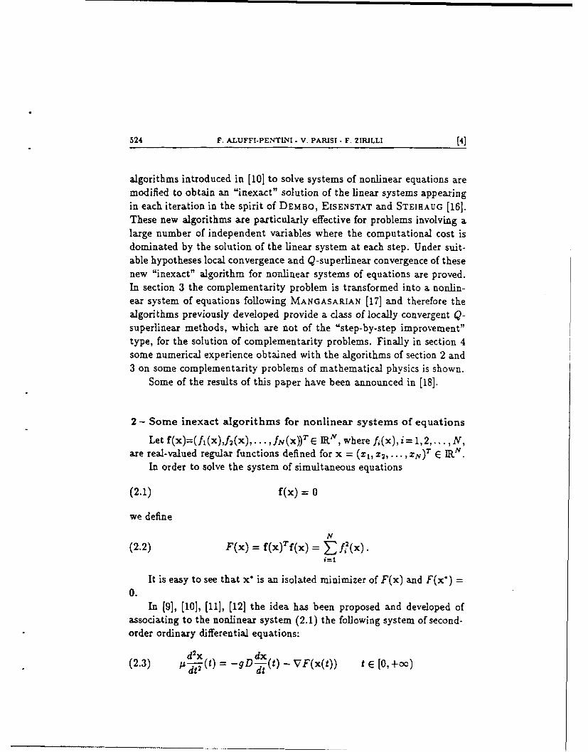
524 F. ALUFFI-PENTINI- V. PARISI -F. ZIRILLI [4]
algorithms introduced in [10] to solve systems of nonlinear equations aremodified to obtain an "inexact" solution of the linear systems appearingin each iteration in the spirit of DEMBO, EISENSTAT and STEIHAUG [16].These new algorithms are particularly effective for problems involving alarge number of independent variables where the computational cost isdominated by the solution of the linear system at each step. Under suit-able hypotheses local convergence and Q-superlinear convergence of thesenew "inexact" algorithm for nonlinear systems of equations are proved.In section 3 the complementarity problem is transformed into a nonlin-ear system of equations following MANGASARIAN [17] and therefore thealgorithms previously developed provide a class of locally convergent Q-superlinear methods, which are not of the "step-by-step improvement"type, for the solution of complementarity problems. Finally in section 4some numerical experience obtained with the algorithms of section 2 and3 on some complementarity problems of mathematical physics is shown.
Some of the results of this paper have been announced in [18].
2- Some inexact algorithms for nonlinear systems of equations
Let f(x)=(fI(x),f 2(x),...,fN (X)) T E RN, where f(x), i= 1,2,..., N,are real-valued regular functions defined for x = (z, X2, . . . ,Zv)T E IR .
In order to solve the system of simultaneous equations
(2.1) f(x) = 0
we define
N
(2.2) F(x) = f(x)T f(x)= ff?(x).i=1
It is easy to see that x" is an isolated minimizer of F(x) and F(x) =
0.In [9], [10], [11], [12] the idea has been proposed and developed of
associating to the nonlinear system (2.1) the following system of second-order ordinary differential equations:
d~x. dx(2.3) y -j(t) = -gD.d-(t) - VF(x(t)) t E [0, +00)
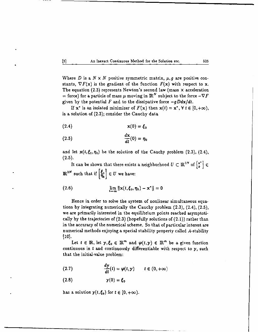
An Inexact Continuous Method for the Solution etc. 525
Where D is a N x N positive symmetric matrix, p,g are positive con-stants, VF(x) is the gradient of the function F(x) with respect to x.The equation (2.3) represents Newton's second law (mass x acceleration= force) for a partide of mass 1A moving in IRN subject to the force -VFgiven by the potential F and to the dissipative force -gDdx/dt.
If x" is an isolated minimizer of F(x) then x(t) = x*, V t E [0, +0),is a solution of (2.3); consider the Cauchy data
(2.4) x(O) =
dx(2.5) dx0) = 7o
and let x(t,fo,qo) be the solution of the Cauchy problem (2.3), (2.4),(2.5).
It can be shown that there exists a neighborhood U C IP2"' of I ER2N such that if ] E U we have:
(2.6) lir lx(t, o, 70) - x11 = 0
Hence in order to solve the system of nonlinear simultaneous equa-tions by integrating numerically the Cauchy problem (2.3), (2.4), (2.5),we are primarily interested in the equilibrium points reached asymptoti-
cally by the trajectories of (2.3) (hopefully solutions of (2.1)) rather thanin the accuracy of the numerical scheme. So that of particular interest arenumerical methods enjoying a special stability property called A-stability[101.
Let t E IR, let Y,e0 E IR' and W(t,y) E IR" be a given functioncontinuous in t and continuously differentiable with respect to y, suchthat the initial-value problem:
(2.7) dy(t) = (t,y) t E (0, +c0)
(2.8) y(0) = 0
has a solution y(t, o) for t E [0, +00).

526 F. ALUFFI-PENTLNI- V. PARISI - F. ZIRILLI (6]
The simplest choice of A-stable linearly implicit method to integratenumerically (2.7), (2.8) is:
(2.9) (I- hD.)(y,+i - y.) = ho. n = 0, 1,2,...
(2.10) yo =
where yn is the numerically computed approximation of y(nh, a), I is
the identity matrix acting on IR', h > 0 is the stepsize, for n = 0,1,2,...
t= = nh, j,, = tny,), 'On = t(t,,yn) where t(t,y) = O5p/Oy is thejacobian of V with respect to y. We note that when 9(t,y) = Ay is a
linear map (2.9) reduces to the backward Euler method.After rewriting (2.3) as a first-order system
dx(2.11) dt - v
(2.12) dv = - I VF(x)dt Y v
formulae (2.9), (2.10) with variable stepsize h,n = 0, 1,... (i.e. to = 0.n-i
tn = _ hi, n = 1,2,...) are applied to (2.11), (2.12), (2.4), (2.5). In thisi=0
case the map (P: IR2N - R T2V will be given by
(2.13) Wp V~ - .Dv - .VF(x)]
so that its jacobian matrix is given by
(2.14) 0(x)= - - D
where
(2.15) L(x) = 2 JxTx + Zf.(x)f(x)]
J(x) = 8f(x)/Ox is the jacobian of f with respect to x and Hi(x) is the
hessian of fi(x).

(7] An Inexact Continuous Method for the Solution etc. 527
Let s,. = x,, x,, n = 0, 1, 2,...; after some simple algebra (2.9)becomes:
(2.16) [L. + 1~ (t-I + gD sv)VF,+]!v
Sn
(2.17) v,+i=, n = 0,1,2,...
(2.18) Xn+i = Xt + Sn
where L, = L(x,), VFn = VF(x,). In order to avoid the computationof Hi(x), i = 1,2,..., N, at each iteration and since we are looking for
Npoints x" such that f(x*) = 0 the term Z f,(x) in (2.15) is dropped so
i= I
that L(x) is substituted by
(2.20) !(x) = 2Jr(x)J(x).
Equation (2.16) will be replaced by
(2.21) A,Sn = b,,
where
(2.22) A(x,h) = L(x) + - [ + gD
and
(2.23) An = A(x,h,)
(2.24) bn = -VF, + -! Vnhn
we note that the matrix An is symmetric and positive definite.We have the foowing theorem:
528 F. ALUFFI-PENTINI - V. PARISI - F. ZIRILLI (8]
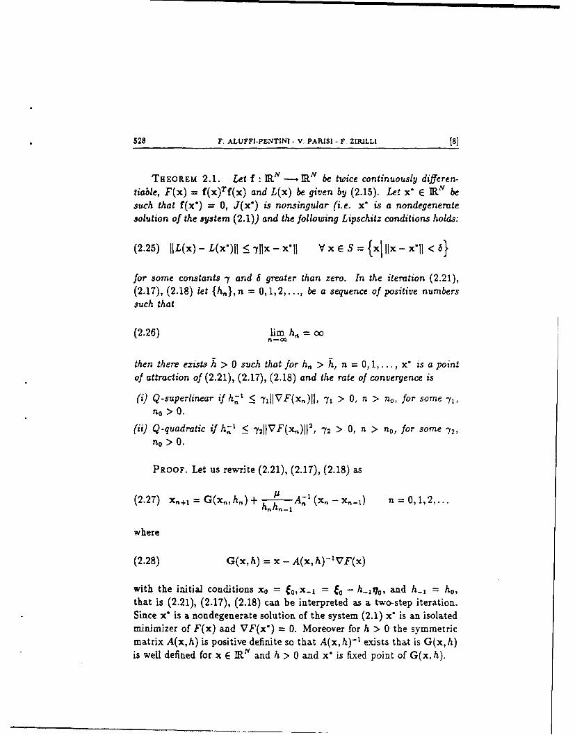
THEOREM 2.1. Let f : IRN - R v be twice continuously differen-tiable, F(x) = f(x) Tf(x) and L(x) be given by (2.15). Let x" E IRN besuch that f(x*) = 0, J(x*) is nonsingular (i.e. x" is a nondegeneratesolution of the system (2.1)) and the following Lipschitz conditions holds:
(2.25) IIL(x) - L(x')ll _ "ylix - xiU V x E S = {xj lix - xl < 6}
for some constants - and 6 greater than zero. In the iteration (2.21),(2.17), (2.18) let {h,,},n = 0,1,2,..., be a sequence of positive numberssuch that
(2.26) lim h,, = oo
then there eziss h > 0 such that for h,, > h, n = 0,1,..., x is a pointof attraction of (2.21), (2.17), (2.18) and the rate of convergence is
(i) Q-superlinear if h- 1 < -tiIlVF(xn), 71 > 0, n > no, for some 71,no > 0.
(ii) Q-quadratic if h; < 72IVF(x, )112, -72 > 0, n > no, for some -/2,no > 0.
PROOF. Let us rewrite (2.21), (2.17), (2.18) as
(2.27) x, +1 = G(xn,hn) + hA A,-,'-(X" - X 1 ) n= 0,1,2"...
where
(2.28) G(x,h) = x - A(x,h)-'VF(x)
with the initial conditions xo = fo,x-I = fo - h-ei, and h-1 = ho,that is (2.21), (2.17), (2.18) can be interpreted as a two-step iteration.Since x° is a nondegenerate solution of the system (2.1) x" is an isolatedminimizer of F(x) and VF(x*) = 0. Moreover for h > 0 the symmetricmatrix A(x,h) is positive definite so that A(x,h) - ' exists that is G(x,h)is well defined for x E IRN and h > 0 and x" is fixed point of G(x, h).

[9] An Inexact Continuous Method for the Solution etc. 529
Let # = JIL(x')-'ll and let 6 E (0,(20) - ') then there exists 6 > 0and h > 0 such that:
(2.29) IIL(x*) - A(x,h)ll !< Vx E S = { X1 lix - X-11 < 6}(2.29) |$
Vh>
In fact
lIL(x) - A(x, h)Il < lIL(x') - L(x)Ul + liL(x) - A(x, h)Il
since L(x*) = L(x*) there exists 6 such that:
IIL(x') - L(x)l <5 1 V x E S
and for a suitable h > 0
(2.30) IIL(x) - A(x,h)ll = IIl + gD < :- V h >h h 2-
From (2.29) and the perturbation lemma (lemma 2.3.2 p. 4 5 of OR-TEGA and RHEINBOLDT [19]) it follows that A(x,h) - l satisfies
(2.31) IIA(x,h)-'Il < V x E S, V h >
Moreover
(2.32) IG(x,h) - x'll < (x,h)llx - x*ll V x E S, V h > h
where
(2.33) w(x) = a [IA(x,h) - L(x)ll + JIL(x) - L(x')j + liq(x)jl]
and
q(x) - I= V(x) - VF(x-) - L(x')(x - x')I1 x x"{ix - x' xx
530 F. ALUFFI-PENTINI - V. PARISI. F. ZZILI (10]
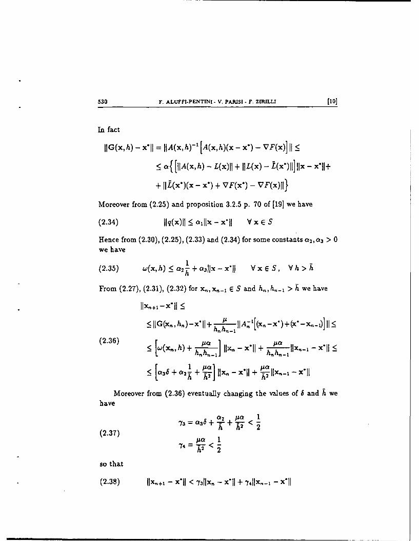
In fact
IIG(x,h) - x'll = IIA(x,h) - [A(x,h)(x- x') - VF(x)] II <
< a{ [lUA(x, h) - L(x)ll + IIL(x) - !(x')ll] Ix - x'll+
+ IIL(x*)(x - x-) + VF(x*) - VF(x)ll}
Moreover from (2.25) and proposition 3.2.5 p. 70 of [19] we have
(2.34) llq(x)ll -<illx - x11 V x E S
Hence from (2.30), (2.25), (2.33) and (2.34) for some constants a2, a3 > 0we have
(2.35) w(x,h) :_ a,-1 + a4l x -xxJ) Vx E S, Vh >
From (2.27), (2.31), (2.32) for x,, x.-. E S and h, h,- > h we have
llx.+,-x'll <
< lIG(x.,h.)-x'll+ h h. A-[
(2.36) <[w(x ,h) + P2] IIjx .- x'll + llx.- - 11 <
[0 3 + C12 + P'] I1 - xII + !- - -X
Moreover from (2.36) eventually changing the values of 6 and h wehave
02 /a0 1
h- + Pa<
(2.37) 3 + h2 2
74=h2 2
so that
(2.38) llxvi+, - x'1l < 731ix. - X'II + - 4 1lXn-i - x'11

[il] An Inexact Continuous Method for the Solution etc. 531
with a4 = 73 + 74 < 1 that is x.+i E S. In particular we have shown that
(2.39) ir x," = X,n , 00
that is x" is a point of attraction of (2.27).In particular for n > no > 0, xn E S, using (2.36) the required
order-of-convergence estimates follows from:
(Ixn+t - x'*j _ [:5 h-. + a3ixf - x'11] Jjx - x'11+(2.40)
1 nIlx
+ Aa 1. - X.- for n o > 0h,,,hn,-1
and the fact that
(2.41) llVF(xn)I -< (IIL(x')Il + c)Jlx. - x'11
where lir En = 0.
Using the method given by (2.21), (2.17), (2.18) requires the solutionof the linear system (2.21) at each step. Computing the exact solutionwith a direct method such as Gaussian elimination is very expensive whena large number of unknowns is involved and may not be worthwhile whenxi is far from x*. In this case it seems natural to solve the linear system(2.21) by an iterative procedure and to accept an approximate solution.In particular since the matrix An is symmetric and positive definite wemay use conjugate gradients. When the method given by (2.21), (2.17),(2.18) is used to solve (2.21) with an iterative procedure, accepting an ap-proximate solution, we will describe this procedure as an inexact method.
Let in be the approximate step computed by the iterative procedurewhen solving (2.21) and
(2.42) rn = An in - bn
be the residual. When rn = 0 the linear system is solved exactly. Letus assume that the approximate step computed in satisfies the followingcondition:
(2.43) lirnli < 4,1IbIl[ n = 0, 1,...

532 F. ALUFFI-PENTINI - V. PARISI - F. ZIRILLI [12]
for some forcing sequence {i3,), n = 0, 1,... We have the following theo-rem:
THEOREm 2.2. Let f : IRvN ---, ]Rjv be twice continuously differ-entiable, F(x) = f(x)Tf(x) and L(x) be given by (2.15). Let x" E JN"be such that f(x*) = 0, J(x*) is nonsingular and the following Lipschitz
condition holds:
(2.44) llL(x) - L(x')l <_ llx - x*'1 V x E S = {xj lix - x'i < 6}
for some constants 'y,6 greater than zero. In the iteration (2.21), (2.17),(2.18) let {hn}, n = 0, 1,2,..., be a sequence of positive numbers and letthe linear system (2.21) be solved approximately in such a way that theresiduals r, given by (2.42) satisfy the condition (2.43) for some forcingsequence {i3 }, n = 0,1, ....If 0 < 4n < 3m < 1, n = 0, 1,..., thenthere exists h > 0 such that if h,, > h, n = 0,1,..., then x" is a point ofattraction of the inexact method (2.21), (2.17), (2.18).
PROOF. Since J(x') is nonsingular and L(x') = 2J(x*)TJ(z" ) wedefine the following norm:
(2.45) Ixl. = IIL(x*)xll V x E I ,
we have
(2.46) 1
where
(2.47) ui = max {IL(x*)ll, IlL(x') - l 1}
Moreover it is easy to see that under the stated hypotheses for anyc> 0 there exists 6 > 0 and h > 0 such that:
(2.48) IlA(x,h) - L(x')il _5 V x E S = {xf lix - x-11 < 6}, h > h
(2.49) IIA(x,h)-'-L(x)-ll< Vx E S = {xjlix-xll < 6}, h >
[13) An Inexact Continuous Method for the Solution etc. 533
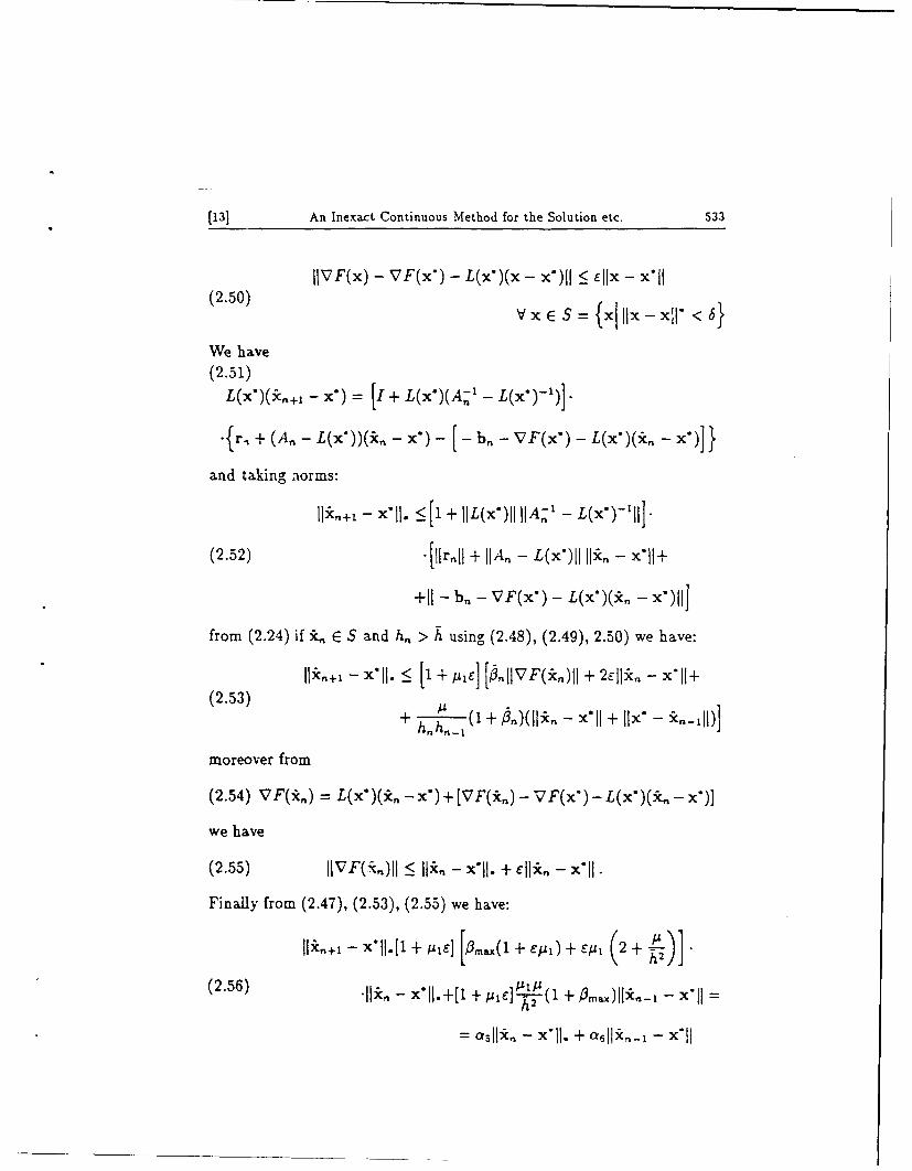
IIVF(x) - VF(x*) - L(x*)(x - x')11: lx - x'11(2.50) Vx s= ES xII~X- x11- < 6}
We have(2.51)
L(X)(R+i- X*) = [I + L(x*)(A- 1 - Lx
-{,+ (A. - LX)(,- X-) - b[- - VF(x*) - L~*(k,- x)j}I
and taking norms:
Il-1- xiI1. 1 [ + IIL(x')I I IA-' - L(XY1-III
(2.52) J{Ir.II + IIA, - L(x')II II-kn - x11l+
+1- b,- VF(x-) - L(x*)(i, - x*)IIJ
from (2.24) if S., E S and h, > h using (2.48), (2.49), 2.50) we have:
lkni- X*1. < 11+ ALE [ flh1vF(k.)II + 2EIi*, -~l
( 2 .5 3 ) + 1 1 + ) I i 0 1 + I X
moreover from
(2.54) VF(i*,) = L(x*)(*,, - x*) + [VF(*k,) - VF(x*) - L(x*)(*, - x*)]
we have
(2.55) lIVF(k'-)l _Ilk, - x11. + _,11i. - x11.
Finally from (2.47), (2.53), (2.55) we have:
- x.[(+I + Epi + Ep, (2 + -!
(2.56) -Ilk. - x11l.+[1 + UJ1ek (1 + X3acI~ - 11 'I
= asll*, - x*ii. + a6 0Ix,1 - xIi

534 F. ALLTFI-PENTINI - V. PARISI - F. ZIRILLI [14]
where
=f [+ /1 1e] [0.m(1 + -C)+i (2 + )(2.57) 6 =2
=i+ Al )(1 + A2(
choosing the values of c and h so that a5 + a6 < I from (2.56) we havethat if *,,*n-1 e S then x,+, E S and
lir n , = Xn-o
THEOREM 2.3. Let f : pN IV be twice continuously differ-entiable, F(x) = f(x)Tf(x) and L(x) be given by (2.15). Let x" E JRN
be such that f(x') = 0, J(x*) is nonsingular and the following Lipschitz
condition holds:
(2.58) IIL(x) - L(x')II :S "llx - x*11 V x S = {xj jjx - x11 < 6}
In the iteration (2.21), (2.17), (2.18) let {h,,}, n = 0,1,..., be asequence of positive numbers and let the linear system (2.21) be solvedapproximately in such a way that residuals rn given by (2.42) satisfy thecondition (2.43) for some forcing sequence {,,,, n = 0,1,...}, such that
0 < n,, <4m. < 1, n = 0,1, .... Then there exists h such that if h,n > h,n = 0,1,...,x* is a point of attraction of the inexact method (2.21),(2.17), (2.18) and the rate of convergence is:
(i) Q-superlinear if h-1 < t7IIVF(n)j[, 71 > 0, n > no for some7, no> 0 and Ur On = 0
(ii) Q-quadratic if h- 1 < -t2jiVF(*.)I2, 72 > o, n > n 0 and ,, <
"t2IIVF(*.)II, 72 > 0, n > no, for some 72, no > 0.
(151 An Inexact Continuous Method for the Solution etc. 535
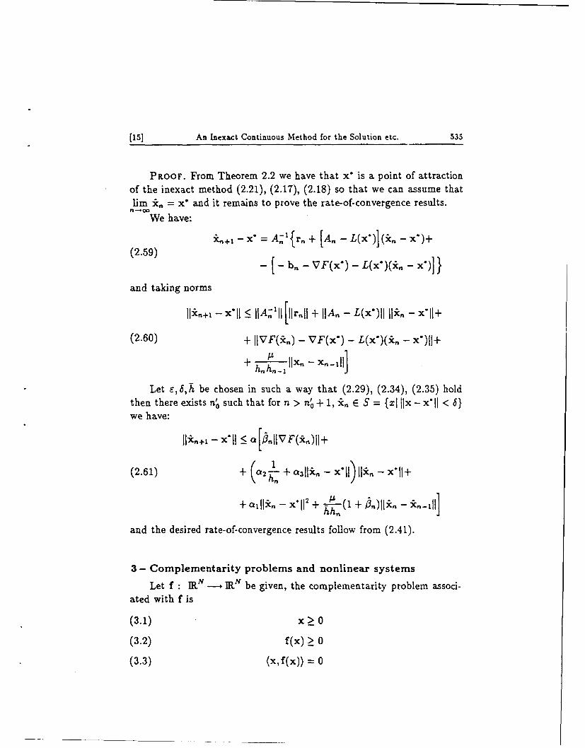
PROOF. From Theorem 2.2 we have that x" is a point of attractionof the inexact method (2.21), (2.17), (2.18) so that we can assume thatlir k, = x" and it remains to prove the rate-of-convergence results.
We have:
kn~ - x A = + [An - L(x*)] kn- X)(2.59)f I(2.59 - [-b, - VF(x-) - L(x-)(in - x-)]}
and taking normsI1kn+l - x1ll _ IIA'II [lirnil + IIA- L(x')ll ilk, - x1ll+
(2.60) + IIVF(*k) - VF(x') - L(x')(:i. - x')ll+
+ A h,---- llx, - X--11]+ hn Ii- ni]
Let e,6,h be chosen in such a way that (2.29), (2.34), (2.35) holdthen there exists n' such that for n > n'+ 1, *, E S = {xi lix-x'l < 6}we have:
[1*.+,- x* :5 a [ .llVF(kn)ll+
(2.61) + (c2+. + k 3lk - x'1l) Ili. - x'i1+
+ Q11. - x'11' + X-(1 + 4.)ll. - kn-ill
and the desired rate-of-convergence results follow from (2.41).
3- Complementarity problems and nonlinear systems
Let f : IR N IR N be given, the complementarity problem associ-
ated with f is
(3.1) x > 0
(3.2) f(x) > 0
(3.3) (x, f(x)) = 0

536 F. ALUFFI-PENTINI- V. PARISI- F. ZIRILLI [16]
and let e : R - IR be a strictly increasing function such that 8(0) = 0.In [17] MANGASARIAN has shown that x* E IRN is a solution of thecomplementarity problem (3.1), (3.2), (3.3) if and only if x" is a solutionof the system of nonlinear equations
(3.4) g(x) = 0
where g(x) =(gl(X),92(X),...,N (X)) T and
(3.5) g,(x) = V(jf,(x) - xI) - (fi(x)) - (z,) i = 1,2,...
for later purposes let us introduce
(3.6) G(x) = g(x) Tg(x)
DEFINITION 3.1: Let x* E IR N be a solution of the complementarityproblem (3.1), (3.2), (3.3) we will say that x" is nondegenerate if x" +f(x-) > 0.
DEFINITION 3.2: Let f be continuously differentiable and J(x) =9f/Ox be the jacobian of f with respect to x, if for fi = 1,2,...,N eachprincipal minor ((Of,/zxj)),i,j =1,2,... , is nonsingular we say thatJ(x) has nonsingilar principal minors.
In [17] 1MANGASARIAN has shown that if x° is a nondegenerate solu-tion of the complementarity problem (3.1), (3.2), (3.3) such that J(x ° )has nonsingular principal minors and o : R ---. IR is a strictly increasingdifferentiable function such that dO/dt(O) + dG/dt(t) > 0, V t > 0, then x °
is a solution of the nonlinear system (3.4) and ag/&x(x*) the jacobian ofg with respect to x is nonsingular.
For simplicity we choose 0(t) = t/2 so that in a neighborhood ofa nondegenerate solution of the complementarity problem (3.1), (3.2),(3.3) the function g(x) given by (3.5) has the same regularity propertiesof f(x). Given the local character of the convergence theorems of section2 this is satisfactory. In section 4 the method for solving nonlinear systemdescribed in section 2 will be applied to (3.4) with 0(t) = t/2 for sometest complementarity problems.
[171 An Inexact Continuous Method for the Solution etc. 537
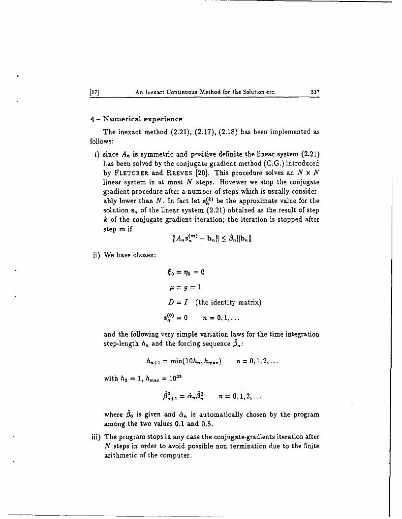
4 - Numerical experience
The inexact method (2.21), (2.17), (2.18) has been implemented asfollows:
i) since A, is symmetric and positive definite the linear system (2.21)has been solved by the conjugate gradient method (C.G.) introducedby FLETCHER and REEVES [20]. This procedure solves an N x Nlinear system in at most N steps. Hovewer we stop the conjugategradient procedure after a number of steps which is usually consider-ably lower than N. In fact let s(') be the approximate value for thesolution s,, of the linear system (2.21) obtained as the result of stepk of the conjugate gradient iteration; the iteration is stopped afterstep m if
IIA~s(-) - b.11 < / .1lb.II
ii) We have chosen:
0= 0 0
D = I (the identity matrix)
ns() =0 n = 0, 1,...
and the following very simple variation laws for the time integrationstep-length h, and the forcing sequence j 3 :
h+= rnin(10h,,hm,) n = 0,1,2,...
with h0 = 1, hma1 = 10"
=n ~ 6 , ,, n = 0,1,2....
where 0 is given and e,, is automatically chosen by the programamong the two values 0.1 and 0.5.
iii) The program stops in any case the conjugate-gradients iteration afterN steps in order to avoid possible non termination due to the finitearithmetic of the computer.

538 F. ALUFFI-PENTINI- V. PARISI - F. ZIRILLI [18]
Finally the method given by (2.21), (2.17), (2.18) (i.e. exact solutionof the linear system (2.21)) is obtained simply setting I0 = 0.
The stopping rule adopted is G(k.) < 10- 1' for the inexact methodand G(x,) <_ 10- 10 for the "exact" method (i.e. i3 = 0). These methodshave been coded in the Pascal programming language and the programhas been run on a Hewlett-Packard 9816 computer.
We have tested the proposed algorithm on three complementarityproblems of which two are linear and one is nonlinear.
The first problem considered arises as a one-dimensional free-boun-dary problem in the lubrication theory of an infinite journal bearing,i.e. a rotating cylinder separated from a bearing surface by a thin film oflubricating fluid [21). The finite-difference approximation used by CRYER
in [21] leads to
PROBLEM A (called Problem 3D by Cryer): Find x, w E IRN suchthat
(4.1) w=q+Mx, w>0, x>0,
(4.2) (w,x) =0
where M = ((Mi)), i,j = 1,2,... ,N, is an N x N matrix with elementsMiy given by
M i = -(H i+ 1/ 2)3 if j=i+1,
M;1 = [(Hi+112)3 + (H_ 112)3), if j = i,(4.3)
M~i = - ( H _- 1/ 2)3 , if j=i- 1,
MA, = 0 otherwise
and q = (ql, q2,... ,qN)T is a vector with elements q, given by
T(4.4) q- N+ [Hi+1
I2 - H- 1I2], i = 1,2,.. .N
where
(4.5) Hi* 1/2 + H i :) T
mmmmmmmm~~~ N + Immmmmm mm

[19] An Inexact Continuous Method for the Solution etc. 539
and the function H(y) is given by1
H(y) = + cos ry) >0
with
(4.7) T=2, E=0.8
We note that the matrix M given by (4.3) is symmetric and positive-definite.
The second problem arises as a two-dimensional free-boundary prob-lem in the theory of the steady-state fluid flow through porous media.Some of these problems can be formulated as a variational inequality af-ter an ingenious transformation proposed by BAIOCCHI and others (ref.[131). The discretization used on the "model problem" ([3], p. 4) leads to
PROBLEM B: Find x, w E IRN such that
(4.8) w=q+Mx, w> 0, x>0,
(4.9) (wx) = 0
where M, an N x N real matrix, and q = (qj,q 2 ,. .. ,qN) E IRN are
defined below.Given n, n. (positive integers) and X, Y (positive real numbers), let
Dz = X/n, + 1,
Dy = Y/n. + 1,
a = Dy]Dx,
let A be the n, x n, tridiagonal matrix having all the main diagonalelements equal to 2(a + 1/a), and the paradiagonal elements (i.e. im-mediately above or below the main diagonal) equal to -a, and let B bethe n,. x n. diagonal matrix with diagonal elements equal to -1/a. Thematrix M is an n x n matrix with a block-tridiagonal structure (n. x n,

540 F. ALUFFI-PENTINI - V. PARISI - F. ZIRILLI [20]
blocks), having each main-diagonal block equal to the matrix A, and eachparadiagonal block equal to the matrix B. We note that M is a positive-definite symmetric matrix. The vector q is defined as follows. Given W(0 < W < Y), and using the Kronecker symbol bij, let
9L (Y) = -(Y - Y)"2
9R(Y) = 1(W - Y), if Y < W,2
9R(Y) =0, if Y>W,
gD(z) = Y 2/2 - (Y 2 - W 2)(x/2X),
gu(z) = 0,riT = -DxDy + iagL(jDy) + bi,,agR(jDy)+
+ b,(1/a)gD(iDx) + 6&,j(1/a)gu(iDz),
i = 1,2,...,n n., j = 1,2,...,n , .
The elements qj,q 2,... ,q, of q are given by
(4.10) qk =Ti, with k=(j-1)n,+i
Our last problem, which is defined below, can be interpreted as afinite-difference approximation of a nonlinear variational inequality.
PROBLEM C: Find x,w E IRN such that
(4.15) w=Mx+p(x)+q, w>0, x>0
(4.16) (w,x) = 0
The problem dimension N, the quantities Dx, Dy and the matrixM are defined as in problem B, given n.,n,,X,Y. The nonlinear termp(x) is a vector in IRN with components pi = x,, i = 1,...,N. Thevector q = (ql,q 2 ,...,q) T is defined by equation (4.10) where ri =
DzDysin(27riDx/X), i = 1,2,...,n=, j = 1,2,...,n , .The numerical results obtained with the previously described meth-
ods on Problem A, B, C are shown in Table 1. 2, 3 respectively.
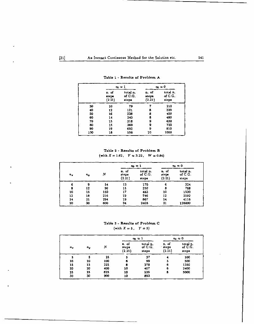
[21] An Inexact Continuous Method for the Solution etc. 541
Table 1 - Results of Problem A
7)o1 10-0
n. of total n. n. of total n.steps of C.G. steps of C.G.(2.21) steps (2.21) steps
30 10 79 7 21040 12 121 8 320so 16 238 8 40060 14 240 8 48070 15 318 9 63080 15 369 9 72090 19 650 9 810
100 18 556 10 1000
Table 2 - Results of Problem B(with X = 1.62, Y = 3.22, W = 0.84)
1o=1 170-0
D. of total n. n. of total n.n, N steps of C.G. steps of C.G.
(2.21) steps (2.21) steps
6 9 54 13 170 6 3248 12 96 1s 250 8 76810 15 150 17 483 10 150012 18 216 19 T46 12 259214 21 294 19 867 14 411620 30 600 34 2405 21 126000
Table 3 - Results of Problem C(withX=5, Y=5)
no_1 ?77 0n. of total n. n. of total n.
nz n. N steps of C.G. steps of C.G.(2.21) steps (2.21) steps
5 5 25 5 37 4 10010 10 100 6 99 5 50015 15 225 8 278 6 135020 20 400 10 407 6 240025 25 625 10 535 8 500030 30 900 10 893

542 F. ALUFFI-PENTINI - V. PARISI - F. ZIRILLI (22]
In tables 1, 2, 3 the adavantage of using "inexact linear algebra" withrespect to complete solution of the linear system for problems A, B, C isshown, and the advantage is increasing with the number of unknowns.
REFERENCES
(1] R.W. COTTLE - G.B. DANTZIG: Complementary pivot theory of mathematicalprogramming, Linear Algebra and Application 1 (1968), 103-125.
(2] F.J. GOULD - J.W. TOLLE: A unified approach to complementarity in opti-mization, Discrete Math. 7 (1974), 225-271.
[3] C. BAIOCCHI - V. COMINCIOLI - L. GuERIu - G. VOLPI: Free boundaryproblems in the theory of fluid flow through porous media: a numerical approach,
Calcolo 10 (1973), 1-86.
[4] G.T. HERMAN: Image reconstruction from projections: the fundamentals of com-puterized tomography, Academic Press, New York, 1980.
[] G.T. HERMAN - A. LEHT - P.H. LUTZ: Relaxation methods for image recon-struction, Communications of the A.C.M. 21 (1978), 152-158.
(6] C.E. LEMKE: Bimatriz equilibrium points and mathematical programming, Man-agement Sci. 11 (1956), 681-689.
[71 E. ALLGOWER - K. GEORG: Simplicial and continuation methods for approx-imating fized points and solutions to systems of equations, SIAM Review, 22(1980), 28-85.
(8] D.A. BAYER - ,J.C. LAGARIAS: The nonlinear geometry of linear programmingI. Affine and projective scaling trajectories, preprint AT&T Bell Laboratories 1986.
[9] S. INCERTI - V. PARISI - F. ZIRILLI: A new method for solving nonlinearsimultaneous equations, SIAM J. Numerical Analysis 16 (1979), 770-789.
[10] F. ZIRILLI: The solution of nonlinear systems of equations by second order sys-tems of o.d.e. and linearly implicit A-stable techniques, SIAM J. Numerical Anal-
ysis 19 (1982), 800-816.
[11] F. ALUFFI-PENTINI - V. PARISI - F. ZIRILLI: A differential-equations algo-riLhm for nonlinear equations, ACM Transactions on Mathematical Software 10(1984), 299-316.
(12] F. ALUFFI-PENTIN! - V. PARIS! - F. ZIRILLI: Algorithm 617: DAFNE-Adifferential-equations algorithm for nonlinear equations, ACM Transactions onMathematical Software 10 (1984), 317-324.

(23] An Inexact W-tinuous Method for the Solution etc. 543
[13] F. ALUFFI-PENTINI -". PARISI - F. ZIRILLI: Global optimization and sto-chastic differential eqtua, Journal of Optimization Theory and Applications47 (1985), 1-17.
[14] F. ALUFFI-PENTINI -V. PARISi - F. ZIRILLI: A global optimization algo-rithm using stochastic O.tntW equations, ACM Transactions on MathematicalSoftware 14 (1988), 34V .
[15] F. ALUFFI-PENTINI -V. PARISI - F. ZIRILLI: Algorithm 667: SIGMA - Astochastic.integration qrminimization algorithm, ACM Transactions on Math-ematical Software 14 (A*), 366-380.
[16] R. DEMBO - S. EIsufAT-- T. STEIHAUG: Inexact Newton methods, SIAMJ. Numerical Analysis 13(982), 400-408.
[17] O.L. MANGASARIAN: lipivaence of the complementarity problem to a systemof nonlinear equations,SUM I. Applied Mathematics 31 (1976), 89-92.
(18] F. ALUFFI-PENTINI -1W_ PARISI - F. ZIRILLI: An inexact continuous methodin complementarity promke, in: Control Applications of Nonlinear Programmingand Optimization, G. dillo (ed.), Pergamon Press. Oxford (1986j, 19-26.
[19] J.M. ORTEGA - W.CREUtNBOLDT: Iterative solution of nonlinear equationsin several variables, Acnimde Press, New York, 1970.
[20] R. FLETCHER - C. DKVES: Function minimisation by conjugate gradients,The Computer Journal ZVI964), 149-154.
[21] C. CRYER: The methdq' Cristopherson for solving free boundary problems forinfinite journal bearingismear of finite differences, Math. of Computation 25(1971), 435-443.
Lavoro perm alla redazione il 23 settembre 1989ed accettatolpr t pbblicazione il 30 novembre 1989su parere fmvole di P. Benvenuti e di P.E. Ricci
INDIRIZZO DEGLI AUTORI:
Filippo Aluffi-Pentini - Dipartia di Metodi e Modelli Matematici per le Scienze Applicate- Universiti di Roma "La SapiA - 00161 Roma - Italy
Valerio Parisi. Dipartimento dr..- 1 UniversitI. di Roma 'Tor Vergata" - 00173 Roma -Italy
Francesco ZiriUi - Dipartimen MtAbamatica "G. Castelnuovo" - Universiti di Roma "LaSapienza" - 00185 Roma - Italy

APPENDIX 2

A Quadratically Convergent Method for Unear Programming'
Stefano HerzelDipartimento di Matematica -G. Castelnuovo'Universith di Rama "La Sapienza-00185 Roma, Italy
Maria Cristina RecchioniIstituto Nazionale di Alta Matematica "'F. Severi"pia.ale Aldo Moro 500185 Roma, Italy
and
Francesco Zirilli
Dipartimento di Matematica -G. Castclnuoto'C:niversita di Roma "La Sapien.a'"00185 Roa. Italy
Submitted b% Richard Tapia
ABSTR-CT
A new method to solve linear programming problems is introduced. This methodfollows a path defined by a sy.stem of o.d.e., and for nondegenerate problems isquadratically convergent.
1. INTRODUCTION
Let R" be the n-dimensional real Euclidean space, andx=(x ..... .r,)Er where the superscript T means transpose. For x.y E R" let xry be the usual Euclidean inner product. and let e ( . .
'The research reported in ths paper has been made possible throuch the support andsponsorship of the Uttd States Cmiernment through its European Re.earch Office of the U S..iny under contract DAJA 45--6-C-0&28 with the Universt di Roma La Sapienza."
LINEAR ALGEBRA ,.D ITS APPLICATIONS 132 2M3-289 (1991) 233
CElsevier Science Publishing Co.. Iw.. 1991655 Aenue of the .lmencas. New Tr NY 10010 0024-3795/91/3.50

256 S. HERZEL N. C. RECCIIION!, AND F. ZIRILLI
A linear programming problem consists in minimizing a linear function overa region defined by linear equality and inequality constraints. We wkill saythat a linear programming problem is in canonical form when it is written asfollows:
minimizecrx (1.1)
Re "
subject to
Ax= 0, (1.2)
erx 1=I, (1.3)
x 0. (1.4)
with side conditions Ae = 0, where
A . ..... in< n.
and c E R" are given, and the inequality (1.4) is understood componentxwlse.that is,
0tl, j1.
Moreover, we assume that the matrix A iz of rank m.We note that on these hypotheses (1/n)e is a feasible point, so that the
feasible region is not empty.The simplex method applies to linear programming problems in standard
form. that is.
minimize dry (1 5)
subject to
Cy b. (1.6)
Y 0. (1.7)
where d E R'. b E R'. C E R"', r 4 s. are given, and the inequalities (1.6).(1.7) are understood component-,,ise. In [11 it has been shown that a linear
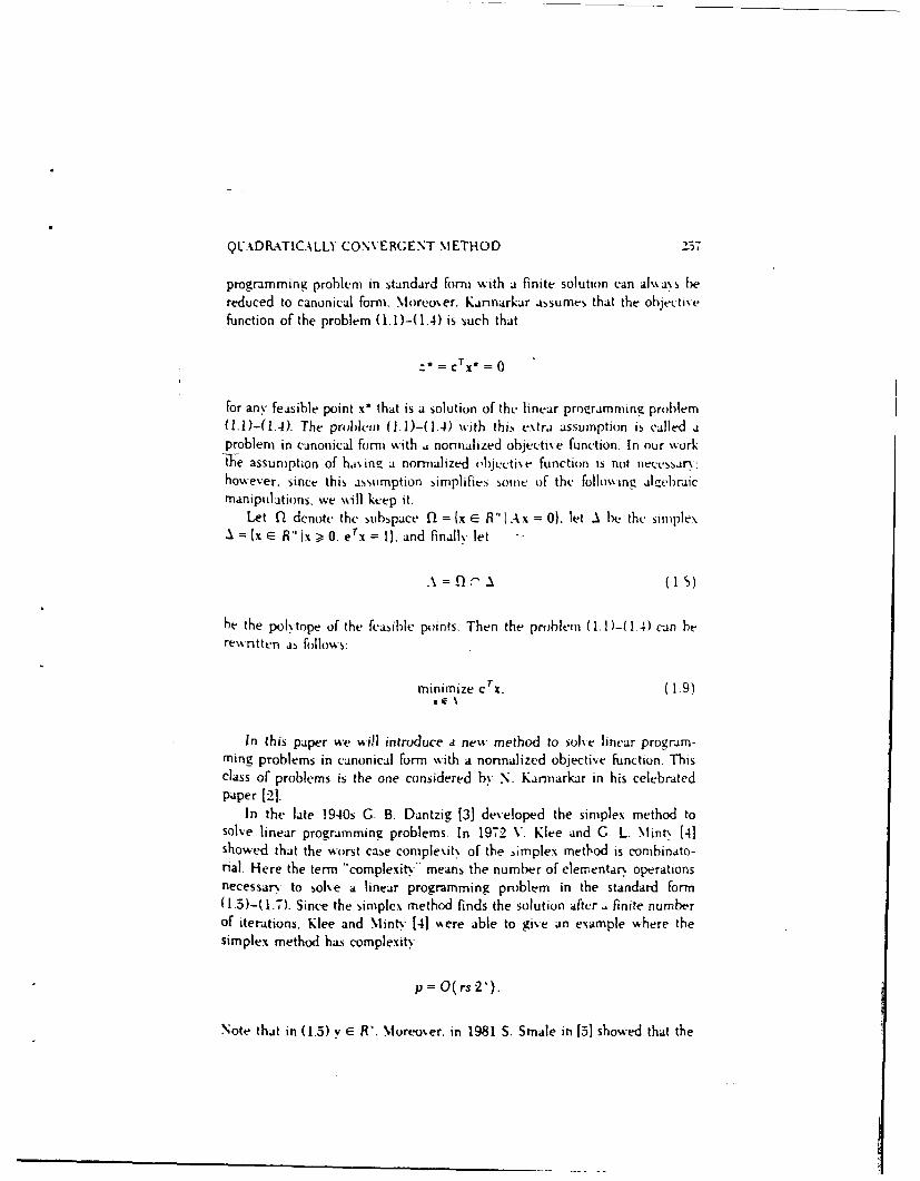
QUADRATICALLY CONVERGENT METHOD 257
programming problem in standard forrii with a finite solution can alwax s bereduced to canonical form. Moreover. Kannarkar assumes that the ohjectivefunction of the problem (1.1)-(1.4) is such that
-Z = cr X*
= 0
for any feasible pint x* that is a solution of the linear proaramming problem1.i)-(L.4). The problem (1.1)-(1.-4) \ith this extra assumption is called a
problem in canonical form with i nornalized objecti\e Function. In our %%orkte assumption of havinz a normalized objectie function is not neQvssarv.however, since this asstmption implifie-. Nome of the folloing alkebraicmanipulations, we \%ill keep it.
Let fl denote the huhspace fl = (x E R"I Ax 0). let .1 be the simplex=(x E R" ix > 0. erx = 1). and finally let "
he the polytope of the feasible p)ints. Then the problem (1.1)-(1.4) can btrevritten as follows:
minimize cTx. (1.9)1 e%
In this paper we will introduce a new method to solve linear program-ming problems in canonical form with a nonnalized objective function. Thisclass of problems is the one considered by N. Karmarkar in his celebratedpaper [21.
In the late 1940s G. B. Dantzig [31 developed the simplex method tosolve linear programming problems. In 1972 V. Klee and G. L. Mint\ [4]showed that the worst case complexit. of the simplex method is combinato-rial. Here the term "complexity** means the number of elerrentar operationsnecessar, to solve a linear programming problem in the standard form(1.3)-(1.7). Since the simplex method finds the solution after , finite numberof iterations. Klee and Minty [41 \, ere able to give an example where thesimplex method has complexity
p = O(rs 2 ').
Note that in (1.5) y e R'. Moreoer. in 1981 S. Smale in [5] showed that the

258 S. HERZEL kI. C. RECCHIONI. AND F. ZIRILLI
"average" complexity of the simplex method is
p = O(rs2 ),
where r, s are the dimensions of the matrix C in (1.6).In spite of its worst case combinatorial complexitv, the simplex method
has been very successful in solving linear programming problems. Thefeature of the simplex method responsible for its worst case combinatorialcomplexity is that it moves on the boundary of the feasible region
Q= (ye R'ICy >b. y >,0}.
In recent years a great deal of effort has been spent in the attempt to find anew algonthin for linear programming whose complexity in the worst case ispolynomial. It is believed that these new methods will go through theinterior of the feasible region Q.
In 1979 L. G. Khachijan [6 introduced the first method of this class,called the ellipsoid metIod. The worst case complexity of this method is
p = O( s').
Here. howe'er, the meaning of the term 'complexity" has been slightlychanged. In fact the ellipsoid method does not step after a finite number ofiterations, so that "'complexity" means the number of eleientar. operationsnecessary to arri,e in a predetermined neighborhood of the solution. More-over, the method introduced by Khachijan is only of theoretical interest,since its practical perfonnance is rather poor.
In 1984 N. Kanuarkar [2] presented a new linear programming method ofpolknomia] worst case complexitY
p=O(s 3 ).
This algorithm is called the projective iethod when applied to a linearprogramming problem in canonical form with a normalized objettive func-tion. This algorithm is of theoretical and practical importance.
Since 1984 a great deal of work has been done in deeloping newmethods for linear programming. Several -interior point algorithms" havebeen proposed. P. E. Gill. W. Murray, M. A. Saunders, J. A. Tomlin. andN1. H. Wright in [7 ha'e interpreted Karmarkar's algorithm as a "logarithmic

QUAD.ATICALLY CONVE RGENT .METHOD 259
barrier method" and have suggested a new algorithm with good practicalperformance.
In the framework of logarithmic barrier function methods we can recallthe work of several authors. In (8] J. Renegar lowered Karmarkar's complex-it%, bound. In [91 C. Gonzaga lowered Rentgar's complexity bound. In [10] M.In and H. Imai. with the hypothesis of being able to perform exact line-searches, introduced a quadratically convergent algorithm for the linearprogramming problem. In [11] N. Megiddo studied the geometr'-al proper-ties of the paths derhed from "weitghted logzarithmic barrier fur rtI(AsFinally, J. A. Tomlin in (121 reports on conniderable numerical experimenta-tion with this kind of algorithms.
In this paper, as suggested by D. A. Bayer and J. C. LUgarias in [13], wewill show that Karmarkar's projectie method can be obtained )y applyingEuler's method with variable stepsize to a suitable initial %alue problem for asystem of ordinan- differential equations. In fact- Karnarkar's method obtainsthe solution x* of the linear programmine problem by computing
Ilira x t. -e (1.10)t-. fl n)
where x(t,(1/n)e) is the solution of a system of ordinar\ differential equa-tions with initial condition (1/n)e, using Euier's method with variablestepsize. The idea of obtaining the solution of nonlinear programmingproblems as limit points of the trajectories of systems of ordinary differentialequations has been widely used, for a review see [14]. In particular, in[15-17] quadratically convergent algorithms for nonlinear systems of equa-tions have been obtained from methods based on the numerical integration oftrajectories of systems of ordinar" differential equations.
The interpretation of Karmarkar's projective method as the numericalsolution of an initial value problem raises two natural questions:
(i) Can the system of ordinary differential equations used in Karmarkar'sprojective method be changed to a new one that will generate an interestingalgorithm?
(ii) Can the Euler method with variable stepsize that is used in Kar-markar's projective method be replaced with some other numerical schemethat will generate interesting algorithms?
An answer to question (i) has been given by D. A. Bayer and J. C.Lagarias in [ 13] and J. L Nazareth in (18], who replaced Karmarkar's vectorfield with the affine eecto,- field. Question (ii) has been considered by N.Karinarkar. J. C. Lagarias, L. Slutsman. and P. Wang in [19]. where they tried

260 S. HERZEL M. C RECCHIONI. AND F. ZIRILLI
to approximate the path .t. (1/n )e) with a power series expansion, obtainingencouraging practical results. In this paper we give two new answers toquestions (i) and (ii)- in fact, we propose a vector field which is differentfrom the ones previously considered, and we use a linearly implicit A-stableintegration scheme (141 to solve the initial value problem considered. In thisway we obtain a quadratic-ally convergent -algorithm for linear programmingproblem. Moreover our algorithm shows good practical behavior.
In Section 2 Karnarkar's projective method is interpreted as the numeri-cal integration of an initial value problem with Euler's method and variablestepsize. Moreo'er. to a linear programming problem in canonical form withnormalized objective function is associated a new system of ordinary differ-ential equations. If we assume that the solution of the linear programmingproblem is unique. this solution can he obtained as the limit point of asuitable trajectory of the system of ordinary differential equations.
In Section 3 an initial value problem for this system of ordinary differen-tial equations is integrated numerically, usine a linearl implicit A-,tablemethod with variable stepsize. It is show-n that this is a quadraticallycof\ergent algorithm for linear programming.
Finall.. in Section 4 we compare the computational cost of our step %iththat of Karmarkar's projective algorithm and that of the simplex alorithm.and we present some numerical experiments.
2. THE USE OF ORDINARY DIFFERENTIAL EQUATIONSIN LINEAR PROGRAMMING
Let xT =(x.x_ ." R "" e gien b% X* =((X,)
Diai(x*). that is. X, = x 5,. i.j = 1.2.... .\here 6, is the Kruneckcrs vmbol.
Dt:Fi\rri0\ 2.1. A minimizer x* of the problem (1.1)-(1.4) is callednondegenerate if it has exactly n - in - I null components.
Let J, = (1.2.. ... and S= (ss ...... s . in I n. be an orderedset of indices such that S g ],,. Let z = (Z -. ..... :,) R be a \ector. Wedenote by z, the %ector z, = (:,,,. z,_) . R -'. Moreover. ,i'en a\,ector v e R"' and a matrix Q E R( ' 1.'" of rank ti - 1. we denote h\ Q\the submatrix Q, = [q".q': .. q""] G R' )"' - 1.. ",w'here qI is the jthcolumn of Q. If B is an ordered set of indices such that B C . andN = A - B. then the sstem
Qz = v (2.1)

QUADRATICALLY CONVERGENT M ETHOD 261
can be rewritten in the following Fom :
QRzB + Q, = . (2.2)
DEFINITIO'N 2.2. Let B be an ordered set of m -- 1 indices. Then B is aset of basic indices for the system (2.2) if there exists a matrix Q' ER(mx"m< - - and a vector , E R" such that the system (2.2) is equiva-lent to the system
z+ , z, = v. (2.3)
LEMM.% 2.3. Let B be an ordered Yet of ti + I indices such that B is a setof basic indicesfor the .systen (2.2). Then Qs IS a?' incertible matrix.
Proof. It folht)ws imnediatelx from the equixalence oF the linear ' stens(2.2) and (2.3). a
Let a>O. x >O. x"= (xrj.x. ...... .,)"ER' . and X"ER. be thematrix X' = Diag(x').
LEMMA 2.4. Let a ; 1 and x" be a nondegenerate minimizer of thelinear programming problem (1.1)-(1.4). Then AX"Ar is an invertible ma-trix.
Proof. Let
.11 = [4] I EE"
be the matrix A with the extra rou,. eT added Since x* is a nondegenerateminimizer of the problem (.I)-(1.4) and Af has rank m + 1. then thereexists an ordered set of m 1 indices B such that xq E R"' has all nonzerocomponents and x.\- E R" - 1 is the zero vector, where N = J. - B. More-over. B is a set of basic indices for the system
Afy = u. (2.4)
where u E R'" is given and y E R Let X;'" E R4= .. x 1 be the

262 S. HERZEL Mt C. RECCH-IONI. AND F. ZIRILLI
matrix x"-Diag~x,*12 ). and XU2X.%*1/2 E fl(n 1~) x(n - ) be the matrix
X.'2= Diag(x.," 2 ). that is. the null matrix. So from Lemma 2.3. Ma E
R~a* ) ( -1)is invertible, which implies that M aX,'1 2 is invertible. More-
over, since B is a set of basic indices for the system (2.4), we have
-(t .I~( BY/M (2.5)
Since MaI*1/ is invertible, from (2.3) it follows that IMX*MT' is invertible,
so that an easy computation shows that AXA AT is invertible. Therefore it
follows that AX *I/ is of rank mn. so that -LX ' is of rank in and AXWAT
is invertible. U
LEMMA 2.5. Let a = I or a = 2. and let x* be a nandegenerate
minimizer of the linear programming problem (IM1-(1.4). Then there existsps >0 such that .X.AAT is invertible for x EES(x*, p*). where S(x,p*)
(x E R" I N~ - x*Il (p8).
Proof. The proof follows immediately from the continuit\, of kX,,.Akr
with respect to x E R'. from Lemma 2.4. and from J. M. Orteea and W. C.
Rheinboldt (20. Lemma 2.3.2. p. 431. E
Let x = (x I Ix .... )r . R". let X E R"" be gi% en by X =Djiz~x): let
D C R'",~ in 4 n. be a matrix, and D the suhspuct!
D - =(x ERIDx=O0). (2.6)
and let n 0A ) he the orthoizonal projection on D -. The projector no0 .alwva\s exists. and if 0 has full rank is gi-'en b%
f1.y=[~rDT )'Dj. v eR". (2.7)
Let r be
r=(x RnIX >.). (2-3)

QUADRATICALLY CUOXEBGENT METHOD 263
and f be its interio.
The set f is called At, positive orthant.For a >0 and xe r let X',' 2 ER'" he the matrix X*
Diag(x*,' 2 .x*,/2 , . 3C:'1). We observe that ,,-. can alw-.ays be ex-pressed in th~e for-m t1). In Fact, let r he the rank of the matrix *AX'V- ifr =mi, then ri AX' -'X- is given by (2.7). If 0 < r < in. we can consider thematrix X E R "" obbied frurm A by eliminating the in - r rows of A withindices equal to thaw of the -m - r rows of .AX* " that are linearlydependent. Since (Ar'I)- vAa2 ) e ha,.e
n(.V ) fl,.. x-. (2.10)
-here f. is c~mby (2.7). Finall%- if r = Owe have that fl.x -,, I-
where I is the n x it idntity matrix Let h.,) E R "he the following vectorfield:
h(x) ~X( I-e T )R Xc). C xR". (2.11)
The vector field h(z) is known as Kannarkars vector field (2. 13]. LetS(x*.p*) be the open ball of Lemma 2.5, and let us consider h(x) for
xEr us(x* p).We obserme that Fi x e f U S(x* p*). AX is of rank n. Then h(x) is a
continuously differenble function of x for x u .. S(x*, p). Let A be giv enby (1.8). and A be Own by
A;= . (2.12)
We will consider the initial value problem
dx- = MO. (2.13)
%(O) - -e. (2.14)n
It is easy to verify do (I/ Oe -

264 S. HERZEL M. C. RECCIIiONI. AND F. ZIRILLI
LE%1M,4 2.6. Let
B= E
be the matrt AX with the extra row eT added, and let y = x/ 'n - 1).
where x e (0.1) is a parameter. For xk E A let
X = Diag(xk). Bk I-e
and let Atk be given by
At ( "~B-(XkC) 11e TX 11 B,-(XL C)) (2.15)
Then Euler's mecthod applied to the initial value problem (2.13). (2-14) trtthvariable stepvize .%tk giten by (2.15) produces thc sequence (xk). k =
0. 1.2..... generated by Karmarkar's alorithin [2. pp. 378-379] applied to
the linear programming problem with normalized objective function(1.1)-(1.4).
Proof. We obser% e that .. tk > 0 for xt . (see [2. Theorem .5. pp.
381-382]. so that. integrating (2.13). (2.14) with Euler's method and variable
stepsize AtI. we ha.e
x"=-e (2.16)II
k' =xk + .. tkh(xi) k = 0.1.2..... (2.17)
The thesis follows from a straightforvard computation. U
For a > 0 let
g(x.a) = fl1. ( X ' 2 c). r r. (2.18)
QUADRATICALLY CONVERGENT METHOD 26.5
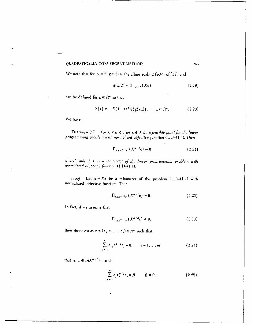
We note that for a = 2. g(x.2) is the affine scaline factor of[1.31. and
g(x.2) - ,..(Xc) (2 19)
can be defined for x C R" so that
h(x) -X(l-eerX)g(x.2). xE R. (2.20)
We have
TIE(-RL\i 2.7 For 0 < a 4 2 let x E k be a feasible point for the linearprogrammow problem with nonnali:ed objecticc function (1.1)-(1.4). Then
fl, ,.(X 2c) =0 (2.21)
.:,..: d i f a , m ,n izer of ic linear programmina problem withnonafl l 1ied .ob 3;ctite functio ( 1.1 )-(1.4).
Proof Let x = Xe be a minimizer of the problem (1.1)-(1 4) withnormalized objecti\e function. Then
R'I.x- )-.(XO/"c) 0. (2.22)
In fact, if we assume that
ln.,x. -,.(X' 2 c) '. (2.23)
then 'hert, exists z = (. .. :,)e R" such that
a,,r , -=0. i= 1. m. (2.24)
that is. z E (.4.LA2 ) and
c)x -' j 2: 0. 8 . (2.25)1-

266 S. HERZEL. M. C. RECCHIONI. AND F. ZIRILLI
that is, X*' 2 c is not orthogonal to z. We can assume without loss of
generality 0 > 0. Let us define
u% = X7/2",: j, 12..... n. (2.26)
Since 0 > 0, there exists j such that wt * 0. If w, 4 0 for j = 1.2.... n. wechoose z > 0: otherwise we choose E as follows:
0<E< a in X (2.27)
j. cc,> 0 W)
We recall that xs > 0 for j = 1.2... n Let
tV = Xj - Ew, j = 1.2.- n. (2.28)
From (2.27) we have
L~j > 0. j= 1,2. n. (2.29)
and
Vtj > 0. (2.30)1'.
Let us define
j= j = 1.2 ..... n (231)
The point u = u ...... u)r is a feasible point; in fact.
Au - 0. (2.32)
e TU= 1. (233)
u > O. (2.34)

QADATICALLY CONVERGENT METHOD 267"
Moreover.
1
e .
--- ( J, - E CXa "2)
n T
= C cJ - E43 = (x ) (2.35)eTv J . I "~ (C
Since x has been assumed to be a minimizer of the linear programmingproblem (1.1)-(1.4) and the objective function is normalized, we have
cT x = 0. (:2.36)
Therefore the objective function assumes a negati'e value at u. and this isabsurd.
Let us assume now that x E A and that Equation (2.21) holds. We willshow that x = Xe is a minimizer of the linear programming problem withnormalized objective function (1.1)-(1.4). In fact. from (2.21) we have
eTxI -*/n -"/20 =' (A ,I)x-- ( " -- 0.(2.37)
Using X instead of A as in (2.10), when A.4X' 2 is of rank less than m wehave
0 = eTX- 1 a-. (X°"O/ 2c)
TerxI-a"[ I Xa.'2r.(. Ar)-'A,*/2JX*':
= erXC-erXAr(AXaAT) -'.kXc = eXc = cTx. (2.38)
Therefore we have that x is a feasible point where Crx 0 , that is. x is aminimizer for the linear programming problem with normalized objectivefiunction (1. )-(I.4). U

268 S. HERZEL M. C. RECCHIONI, AND F. ZIRILLI
Let I be the set given by
= {x E R"IAx = 0, era - 1). (2.39)
LEt.%,. 2.8. Let x* be a nondegenerate minimizer of the linear program-ming problem with normalized objective function (1.1)-(1.4). and let h(x) begien by (2.11). Then we have
h(x*) = 0. (2.40)
Moreover.
Ah(%) = o, X E 1. (2.41)
eTh(x) = 0, x E _. (2.42)
where 1 is given by (2.39).
Proof. In fact for x E 1we have AXe = 0. eTXe = 1. and
AX.-l(,Ax _(Xc) = 0. so that
Ah(x) = - ,-Xfl (Xc) + .-LeeT XFl. X-(Xc) =0 (2.43)
and
eTh(x) =-erxFI(AX)( Xc) +erXeeTXlnx .(Xc) -0. (2.44)
Moreo'er. from Theorem 2.7 %%e have (2.40). U
Let x E R". and E, I R .' .be the matrix gi, en b%
E, = Dia(n,A.,,.(Xc)). x(=-- (245)
Let ]I,(x)e R"" be the folluwing matrix:
Jh(x) = I - XeeT)x'i,.A,(,X- EI-[erx'i .,,_(Xc)]l. xE R
(2.46)
QUADRATICALLY CONVERGENT METHOD 269
For x e R" in (2.46) %%e will use A instead of A. as in (2.10). when A0: is of
rank less than in. An elementar\ computation 5hous that the matrix
x .. can he defined for x E R" so that Jh(x) is defined for x E R".
Let
y = (Xe "IAX2 A is invertible). (2.47)
For x E -. Jh(x) is the Jacobian matrix of h(x) with respect to x. Morteerlet S(x*.p*) be the open ball of Lemma, 2.3: \e obscrxe that for x E t U
S(x*.p*). since AXV is of rank in. the niatrix X1 , \ _X - ' is well defined
and continuous. So Jh(x) is continuous for x E r [ S(x*.p*). and since
l A.(X*c) - 0. we have
]h(X*) = 0. (2.4S )
From Lemma 2S. we conclude that any solution %* of the linear pro'gram-ming problem with nurmalized objective function (1. t)-( 1.4) is an equilib-rium point of (2.1:3). that is. h(x,) -0.
Howe~er. due to the singular Jacobian of h(x) at x* [that is. to (2.48)]. theuse of a linearly implicit A-stable method to integrate the initial valueproblem (2.13). (2.14). as suggested in [8] in the context of nonlinearprogramming, will not produce a quadratically conmeraent method for linearprogramming. To overcome this difficult\ we introduce a new% vector field
x)E R" defined for x e R" given by
f(x)= -(I Xee)[XCXAT(kXkT AXc x eR". (2.49)
where we use A instead of A. as in (2.10). if _LVAT A is of rank less than m.
Let us consider Rx) for x E t.US(x*,p'). We observe that A.'A isinvertible From (2.49) ,e have that fRx) is a continuous]\ differentiablefunction of x for x - r u S(x*. p*). For later purposes %,e observe that Rx) forx E r can be rewritten as follows:
f(x) = -I(i - Neer).x/ 2 l.,( x'l c). xe re (2.50)
Or
f(x) ffi I - X-( - eerX;2 )g(x. 1), x er. (2.51)
From Equations (2.20). (2.51) and Theorem 2.7 it follows that if x" is a
kd
270 S. HERZEL M. C. RECCHIONI. AND F. ZIRILLI
minimizer of the linear programming problem. then f(x°) = h(x°)= 0. that is,x* is an equilibrium point of the vector fields h(x), Rx). For x E A the vectorfield Rx) can be obtained as the steepest dcscent vector associated to thefunction crx with respect to a particular metric. [n [13] D. A. Bayer and J. C.Lagarias have introduced the idea of looking at Karmarkar's vector field h(x)in terms of steepest descent directions.
Let x, be a feasible point of the linear programming problem (.1)-(1.4),and Fo be the affine subspace
F, = X0 + (v E a "'Av = 0. eTV = 0). (2.52)
LEM--I 2.9. The cector fwld Rx) given by (2.31) is the steepest descentrector associated to the objective function b(x) = cTx of the linear program-ming problem (1.)-(1.4) restrtcted to F. r) t with respect to the Riemannianmetric G(x)= X-' = Dag(x-'). defined on the positive orthant r. where F.is giren by (2.52).
Proof. We consider the following transformation for x E F, n F.
G X"'2 . (2.53)
We have
b(,(.v)) X 2 \x-c,! T v, " "'
and Fo assumes the following form.
FO =., -,(u -R"AX u = 0. erX'I"u-0}. (2.5)
The gradient ,,ector of b(x(. )1 .ith respect to y is
ab= x1/2c. (2.56)
The gradient vector ab/dy projected on ' j is gi.en by
4l= n AN , , ]. x ' : ) (2.57)

QUADRATICAL Y CONVERGENT M ETHOD 271
where we use A instead of A. as in (2.10). if A.XA' is of rank less than in.Since -tXe = 0 from (2.57). using (2.7) we have
S= X'I,2 c- X I I AT('AXT) - I.k:c- X I/2eeTXc. (2.58)
Since erXAT(AXAT) - IAXc = o, we have
g= (- Xi/ 2ee r x ,/2 )fl.x _.,_(X 2c). (2.59)
Finally. appl\ing (2.53) to g. %%e have that the gruditnt \ector ;(x) is gikenby
;(x) =X "- X ,'2(tI_-X l ' "-2ee X ') , \ :. X1 c) (2.60)
This concludes the proof. U
Let A be gi'en b\ (.3).
LExlx,. 2.10. Let x E A. and r be the rank of die matrix kXAkTA. Then
F1 ,21 ,(X'i 2 c) =(I - X: " r-2) (X' -c), (2.61)
where we use A instead of A. as in (2.10), when r is less than in.
Proof. Let 0 < r 4 m. The projector l AX' I- is defined as follows:
(2.62
n[ .l 2 ([eX 12 ' 2 ] T 1X' -2]- 2
Let us compute the matrix
1/2 1"e Tx1X/2 ieX 1/2

272 S. HERZEL M C. RECCHIONI. AND F ZIRILLI
Since AXe = 0 and erXe = 1, we have
(A'XAr) I . (2.63)
An elementarN computation gives us
n[ X1,,:(x"2 c) = x"-c- X I'AT(.4AAT)'. \Xc- X1/2eeTXc. (2.64)
From er.AT = 0 we have
q = XI/leeTx AT( .AT) A_c 0 (2.65)
and
I 2]] -( (X'c) = fl.., :.( X-c) - Xu/2 eerXl/2 c -q. (2.66)
With an eas' computation from (2.66) me obtain (2.61). Let r = 0. and0 e R .. be the null matrix. We ha -c that
[ OT 1 2 = (e X ' ) - and ri 0. = 1.
so that (2.61) holds. U
LEt\,'i'i 2.11. L't x" be a'nonde'generate minimizer of the lincar pro-graurnio problem w'ith nonnalized objectice fjnction (1.1 )-( 1.4)Y let ffx) begiven by (2.49) and 1 be given by (2.39). Then we hate
f(x.) = 0 (2.67)
moreoter
Af() =0. x E 1. (268)
erf(%) =0. x E 1. (2.69)

QUADRATICALLY CONVERGENT M ETHOD 273
Proof. Let a = 1. From Theorem 2.7 we hae
[I.&x.,' ( X~l'c) = 0. (2.70)
so that
f(x*) =0. (2.71)
Let x e 1. Since ALe = 0 and erXe = 1, we have
Af(x)= -(A -.-XeeT)I X[c- x.AT(AXAT) -'.aXc]= 0 (2.72)
and
eTf(x) = -(er-erXee T)[xc - N:,T( A X_T )-'.c] =0. (2.73)
This concludes the proof. U
LE 1%1-, 2.12. Let R x) be given by (2.49). and x, e R' be such that
Ax 0 = 0, (2.74)
eTxu = 1. (2.75)
Then the solution x( t) of the initial talue problem
dx-T = R ). (2.76)
x(O) = x0 (2.77)
satisfiAW the constraints
Ax(t) = o, (2.78)
erx(t) = 1 (2.79)
for all values oft where x(t) is defined.

274 S. HERZEL, M. C. RECCHIONI. AND F. ZIRILLI
Proof. From Lemma 2.11 we have
dxA-- Af(x) =0. (2.80)
Tdtrd x
e - erf(x) = 0, (2.81)
so that the thesis follows immediately from the assumption (2.74). (2.75) onx0 and the fundamental theorem of calculus.
For x E R" let E E R"" be the matrix given by
E = x R . (2.82)
and C E R" " be the matrix C = Diag(c). Let J(x)- R" Xn be the followingmatrix:
(x)=[t--T(.XAT)'AXeer](C-E)(erX)l .- R".
(2.&3)
where we use A instead of A. as in (2.10). if A.XAT is of rank less than m.Let Y' be the set (2.47). An elementary computation shows that for x e Y,/(x) is the Jacobian matrix of Rx) with respect to x. Moreo\,er let S(x*, p*) bethe open ball of Lemma 2.5. We observe that for x E f U S(x*. p*). since thematrix _AT is in~ertible, J(x) is continuous for x E r U S(x*.p*).
THEOREM :L13. Let us assume that the linear programming problem(1.1)-(1.4) has a unique nundegenerate minimizer x*, and let J(x;) be gitenby (2.33). Then J(x*) is inrertible as an operator restricted to the subspace[A1. That is. J(x*)v 0 for each v*O such that
e r 4
QUADRA TICALLY COWUGENT METHOD 273
Proof. First of aiw show that for i = 1.2 ..... n we have
(C-E),. 0 if and only if x, * 0.
Let X" = Diaq(x'). FumTheorem 2.7 for a = I we have
X, -E) Di((f . (.'" ))) = 0. (2.S4)
Since C - E is a diam matrix. from (2.S4) we have that X,, r 0 implies(C -E),, = 0 for i =NL....n. Let us show that (C - E),, = 0 impliesX,* : 0 for i = 1,2.. w In Fact if we assume that there exists h such that(C - E)I,h = 0 and x,*-= then from the assumption that x* is a nondegen-erate minimizer of thelmrr programmina problem (1.1)-(1..4) it follows thatthere exists a pivot tisformation that makes the hth component of x*nonzero. Let v* be tlb"ww basic feasible solution correspondiniZ to x" viathe pivot transformatimL Since onl% one pi-tot operation has been made. thenonhasic componentsier than the hth component are still nonbasic. thatis, y,* = 0 for each i *4 such that x,* = 0. Let Y*= DiaL.,( y,*yy).From (2.S4) we have
Y-(C- E)=o. (2.S5)
Moreover, since eT' .- 0. from (2.85) we have
0=eTy*(C - E)e=JTIaCe-eTY*AT(.-U*. ) : A"c=eTY c=cTV* .
(2.86)
Therefore y* would heanew minimizer of the linear programming problem(1.1)-(1.4). different fit z. and this is absurd.
We have J(x*) - =C - E)-. In fact it is obvious that v E (C - E)implies v - J(x*)-. Nm'er. let
.A, +rXA( . T a ) -'A _-eer] (C - E). (2.S-T)
Then
tIm(()- ( - E) -X *M, (288)
SO that J~' -0 imlln (C - E)v - X *My . Since N' is a diagonal matrix.

276 S. HERZEL M. C. RECCHIONI. AND F. ZIRILLI
we obtain (X*Mv), = (X),(Mv),. i = 12..... n. We have two cases:
(i) X,; = 0. which implies ((C - EM, = 0:(ii) X,*, 0, which implies (C - E), = 0.
Summarizing, we have that ((C-E)=),=O, i=1.2.....n. that is. vE
(C- E) "Now let u E R n be such that
Au = 0. eru = 0. (2.$9)
We assume that u ( J(x*) -: since x* e (C - E) -, then z = x* + u E J(x) ..Moreover.
Az = 0, eTz=1, (2.90)
and z-J(x) - implies zE(C - E). If z E(C- E)-. then z, =0 for eachi such that x," = 0: this condition. together with (2.90). is a characterizationof the minimizer x* of the linear programming problem (1.)-(0.4). There-fore u = 0. This concludes the proof.
TiE, RE\, 2.14. Let x* be the unique nonde,-enerate rinimi:er of thelinear programming problem with nonalized objectice function (L.1)-(1.4).and RX) be given by (2.49). We consider the initial calue problem
dx- = fx). (2.91)dt
1x(0) = -e. (2.92)
Then a solution x(t.(/n)e) of (2.91). (2.92) exists for t E [0.x). and
rm x t. -e = x (2 9.)
Proof. The standard existence and uniqueness theorems for the initialvalue problem for ordinary differential equations guarantee that the solutionof (2.91). (2.92) exists locall, From Lemma 2.9 it follows that Rx) is

QUADRATICALLY CONVERGENT METHOD 277
tangential to 8.A. so that from Lemman, 2.12 and the fact that (l/n)e E .' weo
have that x(t,(I/n)e)e A. Moreover for x E A we hae
d.) T d I y c X .e~ c - -Ix -c <0. (2.94)
that is. the objective function crx is monotonicall\ decreasing along thetrajector. xt.(l/n)e). Since the minimum of crx on A is zero. x* is theunique minimizer of crx on A. and Rx*)= 0. from G. Sansone and R. Conti[21, p. 311 we have that x* is the unique limit point of xt.(l/ne) and
lim xt, e)=x. (2.95)
This concludes the proof .
3. THE QUADRATIC ALGORITHM FOR LINEAR PROGRAMMING
Let X ( Rn. Dc R" be an open set. and D be the closure of D; letw: D c R" - R" be a function continuously differentiable in D. whoseJacobian matrix is denoted by Q(x} - w/ax. Let us consider the initialvalue problem
dx- = ,(,). (3.1)dt
x(0) x,. x41 e D. (3.2)
Let I be the n X n identity matrix. hj > 0. k = 0.1.2 ..... be a sequence ofstepsizes. and tk E h, Then any solution x(th) of (3.1). (32) can beapproximated with xi computed as follows:
X (I, X0. (3.3)
[1-h,Q(,,)1s ,- hw(xk) k - 0. 1. ... (3.4)
X'k' m X +sk. k -0. .2.... (3.5)

278 S. HEP.ZEL M. C. RECCHIONI. AND F. ZIRILLI
The numenc-a] scheme (3.3)-(3.5) to integnte the initial value problem (3.1),(3.2) is A-stable and linearly implicit, and has.heen studied by J. D. Lambertand S. T. Sigurdsson in [22.
Let R) be the vector field given by (2.49), and J(x) be its Jacobianmatrix given by (2.83). We will apply the numerical scheme (3.3)-(3.5) tothe initial value problem
dx-T = X). (3.6)dt
X(O) = -C (3.7)n
considered in Section 2. Let t be gien by (2.9). B%, Lemma 2.5 there existsa neighborhood S(x.p*) of x* such that Rx) is a continuously differentiablefunction in F . S(x*.p*).
LE'.,ta. 3. 1. Let x* be the unique rninitnzer of the linear programmingproblem with nurmali:ed objective functun (1.1)-(1.4). Let us apply thenumerical schemc (3.3)-(3.5) to the initial ralue problem (3.6). (3.7). More-oLrr let
h,*(erXc) - ' for k = 0.1.2.. (3.S)
l-hj(xk) beinvertible for k =0.1.2... (3.9)
Then the sequence (x -I, k = 0. 1.2..... g ncratcd by (3.3)-(3.5) exists. andsk satisfies
Ask ="0. k = 0.1.2.. (310)
eTs =0. k =0.1,2. (.3.11)
Proof. We note that %"=(l/n)e is a f. oible point of the linearprogramming problem (1.1)-(1.4) and that s' is defined by
[I- h1j(x's' - hkf(,) k 0.1.2....
In Lemma 2.11 it has been shown that if z' is a feasible point for the linear

QUADRLATICALLY CONVERGENT METHOD 279
programming problem (1.1)-(.4), we have
Af(xk) =0, (3.13)
e'f(xk) - 0. (3.14)
so that applying A to both sides of (3.12). we obtain
A[I- h&J(xk)I sk = 0. (3.15)
From (2.83) we have
.AJ(xk) = (eTX~c)A. (3.16)
Therefore %-e have
I - h k(eTXk c)lAs' = 0. (3.17)
so that from (3.8) we have As' = 0. k = 0, 1.2.Mloreo, er it is easy to yen fv that
eTj(xk) -(erXkc)eTI. (3.18)
SO that from Lemma 2.11 we have
J[I- h&J(x&)I sk = 0. (3.19)
which implies
[ I- h, (erX, c)]Iersk = 0. (3.20)
SO that from (3.8) we have eTSk 0. k -0. 1,2,..
Let D C R" be an open set and Do C D be a con% ex set.
DEFINITIo% 3.2. Let w(x): D 5;R - R* be a continuously differen-tiable finction. Let 9 r= R'. DI be an open neighborhood of 4, and T: D x
D4C R" X R- - L(R-). where W")I is the set of the n X n matrices. ThenT(-is a consistent approximation to the Jacobian matrix Q(f of w(x) on

280 S. HERZEL . C. RECCHIONI. AND F. ZIRILLI
D o c: D if 0 E R' is a limit point of D, and
lira T(x,. Q(x) (3.21)
1-0teD4
uniformly for x E Do. Moreover. if there exist two constants c > 0 and r > 0such that
IIQ(x)- T(x. 9)I V 1< i. (3.22)
for each x E D,, and 4E D,(S(O.r), where S(O.r)=(g e R"'Ii;I < r,then T(x. g) is a strong]y consistent approximation to Q(x) on D,.
LE\\i,% 3.3. Let DgRn be an open set. and w: DC_ R"- R" be acontinuously differentiable function on the convex set D, C D. Let QW )ELip,( D,). that is. let Q() be a Lipschitz continuous function for x E DU withLipschitz constant y ;: 0. Then
y-1 (y) -w(%) - Q(x)(.v- -)!I1 'Y -;'x - yil" (323)
for each x. v E D,
Proof. See J. M. Ortega and W. C. Rheinboldt [20. Theorem :32.12.p. 73]. U
Titi)Rt,,i 3.4. Let x* be the unique nondezc'ie'rate minimizer of thelinear pro,.rainming problem with normalized obiec:iue function ( 1.1)-(1 4).and let
and B - be zrteii by (2.S). Moreover. let fR) be gicen by (2.49). and
h= R%, k = 0. 1 2..... (324)
where a, > a>0 is a bounded sequence vuch that h= * (eTX c) "'. Then

QUAD FATICA L LY DiMGENT,- METHOD 281
there exists p, > OM open nei h orhood S(x*.p,) = x e R"lJ - xi*N <
p,) of x" such thalt. eS(z.p,)r . uwhere 1 is given by (2.39). then thesequence xT k =M . am- rated by
x" = ,,.(3.2.)
[I - h,.dz-' -,r ) = hi R(x ). k = 0.1.2 ..... (3.26)
where J(x) is W,_iten M) and the lineur system (3.26) is suh ed in B -. iswell defined. x ' *Wp)ll 1 for k = 0. 1.2 ..... and x). k = 0.1.2 .....conteres quadratic" e.
Proof. We arsoiduction on the index k. Let
I& k =0.1.2.. (3.27)
and
c(. J+ - t+J(x) k =0.1.2... (32S)
We observe that (3io be re'ATitten a folows:
- (- -x I) = f(XP ). k = 0.1.2..... (3.29)
It is eas\ to see tli&) is a strongl. (.otnistent approximation of J(x) onf when f goes toam We hae seen in Lemma 3.1 that if v E R' andXK e we have
, ,,. (e) X = Ce'x, - f, )AV, (3.30)
".'.f), = (e'.,, c - fk,)e TV.(3.31)
From (3.24) and CM Dows that , * eTXkC for k = 0.1.2,..., so thatwe have
41JE B- if and only if v E B. (3.32)

282 S. HERZEL M. C. RECCHIONI. AND F ZIRILLI
From Theorem 2.13 we have that J(x*) restricted to B " is invertible and
111[J(,*)]18i2[J(,,.) - ow-,, l is )11.] < 1 (3.3)
for xk e S(x*,p,) in a suitable neighborhood of x* and fk in a suitableneighborhood U of zero. The perturbation lemma (see J. M. Ortega andW. C. Rheinboldt [20, Lemma 2.3.2. p. 45]) implies that the inerse of thelinear operator (xk,) restricted to the subspace B exists when xk E
S(x*,p 1 ), C, r U. From Lemma 2.11 we have that x k E implies R1 &) E B -.When x k S(x*.pj)r)! and k EL', from the fact that R&)E B - and(3.32), (3.33) it follows that x-' is well defined and xk -' -. Moreoverthere exists -q7> 0 such that
and we have
Nb - -,.1 = II(,.,1-[(' ,), ,)-f,)
-4 7(11 O W , )J - J( x , )11 + 1l A x 1) _ P (x .* 1 x ,
+ ,77i f(x*)- f(x) - J(x*)(k -)x*)i. (3.35)
Since we can always choose pI > 0 such that J(x)C Lip.(S(x p,)) for somey > 0. from Lemma 3.3 we ha%,e
' -*ll < .,77tl -x:l+ 7y1, % -xi*- + -X- 12
4 W(KI , k -" XI l (3,36)
where
w(x',k)= 17fk + 17YIIXk -xll. (.3.37)
The neighborhoods S(x'.p,) and U can be chosen in such a wa, that
W(X , - ,X< 1. 1kEs( p,)n*. . (3.38)

QUADRATICALLY CONVERGENT METHOD 23
From (3.36) and (3.38) we have
X411 -x < XU'x -. 01. xL. (- S(X'. P,) r) 1. (3.39)
Therefore xk- I E S(x*.p,)r ) . Moreuer 'we have
!Ix -x*I < x, -lix" - xIL, (3.40)
so that the iterates (W), k = 0. 1.2 ..... given by (3.26) --e well defined ifx" E S(x*.p )n 1 and
lim xL = x*. (3.41)
Moreover. since Rx) is a c ntinuouslk differenitiable function in a neiahbor-hood of x* and Rx*) = 0. there exists a constant .1 > 0 such that
If(x)I..~xL-xii. xL ES(.X ,) (3.42)
From (3.24) ,e obtain
fk < E=- -~ l, x S(x*. , ) n r) . (3 .43)
That is. the sequence x&) converges quadratically to x'. This concludes theproof
4. NUMERICAL EXPERIMENTS
We begin b% comparing the computational cost of a step of the algorithmintroduced in Section 3 with that of a step of the simplex algorithm or of a
Step of Karmarkar's algorithm.We consider the linear programming problem in the canonical form
(1.1)-(1.4). It is easy to verify that the computational cost of a step of thesimplex algorithm is given b%
mn + lower order terms (4.1)
28-4 S- HERZELS M C. RECCHIONI. AND F. ZIRILLI
The computatin~os of one step of KArrnarkar's algorithm is essentiallydue to the computiof the matrix
.A.X2 AT (4.2)
and to the solution Affi mX mn linear system
(.A?2.Ar,)v = -LVC. (4.3)
Since the matrix AM i s svmmetric. its computation requires
m 2n-7-+ lowver order terms (4.4)
elementary operatm while the solution of the linear systen (4.3) requires
M I- + lowver order terms (4[.3)6
elementary operatim Since m < n. we c-an conclude that the computationalcost of one step offismrkars algzorithm is rouizhl%
in+ low-.er order terms (4.6)
elementary operatn This cost can be reduced using somne special proce-dures. for examplum W1 Karrnarkar has show,%n that the use of sucessikerank-one mod fcai t compute (4.2). (43) reduces the -a'erace- co)mpu-tational cost of eaclp to
cnl- - lo"ver order terms, (4.7)
elementary opertm for some constant c > 0.The computatidkot of one step of the algorithm introduced in Stcction
3 is essential% duea~e computation of the matrix
(4.S)
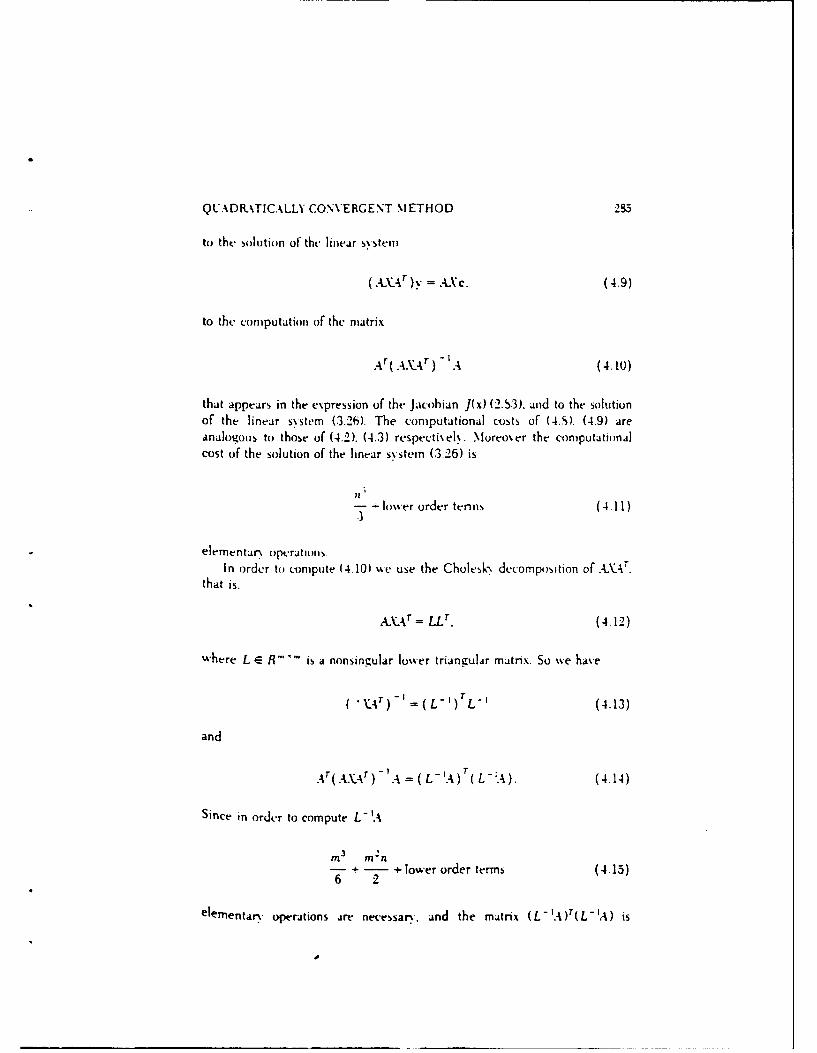
QLADR-TICALLY CONVERGENT METHOD 2S5
to the solution of the linear s5steni
(.- - r )y = .- 'c. (4.9)
to the computation of the matrix
Ar( AXA r ) -tA (4.10)
that appears in the expression of the Jacobian J(x) (2.S3). and to the solutionof the linear s.stem (3.26). The computational costs of (4.S). (4.9) areanalogous to those of (4.2). (4.3) respectivelk. Mureoer the computationalcost of the solution of the linear systein (3.26) is
- lower order terms ( 4.11).3
elementan opcrations.In order to compute (4.10) we use the Cholesk? decomposition of _L\LAT.
that is,
,L"A-r = LLT . (4.12)
where L E R'... is a nonsingular lower triangular matrix. So we have
S,AT)- = ( L - (4.13)
and
At( AA r ) - 'A - ( L-.)T(L-A). (4.14)
Since in order to compute L -'.A
m 3 mn1n
- + - + lower order terms (4.15)6 2
elementary operations are nevensar%., and the matrix (L-.A)(L-A) is

286 S. HERZEL M C. RECCIIIONI. AND F. ZIRILLI
symmetric, the computational cost of (4.10) is
m2ri- + lower order terms (4.16)2
elementary operations. Since m < n. we can conclude that the computationalcost of one step of the algorithm introduced in Section 3 is
1.3 3J-n+ lower order terms (4.17)
elementary operations. Moreover, if we use successive rank-one modifica-tions, as proposed in [2]. we can decrease the "average" computational cost ofeach step to
c'n2 s + lower order terms (4.1S)
elementary operations. for some constant c'> 0. Moreover. to improve thevalue of c' it is possible to use any combination of the ideas proposed in (7.2.3. 241.
To conclude, the computational cost of one step of the algorithm intro-duced in Section -) is of the same order as that of ore step of Karmarkjrsalgorithm, while one step of tlk, simplex aliorithm is much cheaper. Hov.-ever, due to , .'.idratic convergence of our algorithm. .e expect that thenurbe- f it-. .ns needed to solve a linear programming problem to agiven accuracy should be approximatel\ indept-ndent of thc problem size n.
We present now some numerical results that support our expectationThe algorithm described in Section 3 has been implemented using t ,ospecial expedients to a~uid failure due to the ill-conditioning, of the problemconsidered.
The matrix A E R" ". zi'en by (1.2) is replaced with the matrix A C-R .... to reduce its condition number. A is obtained usine the singular %aluedecomposition of LAr This decomposition has a computational cost of ord rn 3. so it costs the same as one step of the alzonthm described in Section 3Let AAr= QrDV, be the singular value decompositon of .Lr: then the
matrix A is given b,
A = (QrDV).)A. (4.19)
where D E R.... is a diagonal matrix such that ( D'),, = I/D,, if D,, >0and(D),,= Iif D,=0 for iL ....

Q.ADR.TICALLY CONVERGENT .IETHOD 287
In the first k1 steps of our algorithm (k1 .5 in our numerical experi-ments). the Riemannian metric
G(x) = X - ' = Diag(x - ') (4.20)
is replaced with
C1(x) MkX (4.21)
where M, = X = Diag(xi - ) and xj is the current point at step k. We notethat in order to apply our algorithm is not necessary to ha-e a normalizedobjectixe function-that is. is not necessary to kno\\ the ,alue of theobjective function at the minimizer. Hoexer. in our numerical experimentswe use test problems with normalized objective function. The stopping ruleused is
v/k=crx _< 1.OX -10 c _). (422)n
We have considered ten tcst problems Problem 1 (Z I R 1) is a problemcoming frrom the operation of an industrial plant in central ltal\,. The otherproblem+ come from the S\stem Optimiz-ation Laborator\ at Stanford Uni-versitv and have been made a\,ailable to us through \ETLIB [25]. Thenumbers of variables (n) and of constraints (in). show-n in Table 1. are thoserelative to the problems in canonical form. Finally, k denotes the index of thefirst step that verifies the stopping rule (4 22).
We note that in Table 1. while n. m %ar by an order of magnitude, thenumber k of steps needed to solve the problem varies only b% a factor of two.Moreover. test problems with n. in < 5 are solved in about ten steps.
TABLE I
Test problem m n k V,
1. ZIRI N304 _43 21 2 .4l1-102. ADLITTLE 57 141 21 3 .16r-093 AFIRO 2S 54 12 1 52t-124. SEACONFD 173 2- 20 3. 9 1D-093. BLEND 75 117 21 1.47 -126. ISRAEL 175 319 17 1.94D-107 SC105 106 166 13 1.36n-1S. SCSOA 51 51 14 1.48r-149. SC5O 51 81 11 7 .S-4&-10
10. SMARE2B 97 167 21 1.7 8D-10

288 S. 1IERZEL, N1. C. RECCIIIONI. AND F. ZIRILLI
The algorithm has been coded in FORTRAN and tested on a VAX/VMSVersion V5.1 in double Precision arithmetic.
REFERENCES
I N. Hooker, Kanisarkar's linear programming algorithm, Interfaces 16:75-90(1986).
2 N. Karrnarkar, A newv polynomial time algorithm in linear programming. Combi-natorica 4:373-395 (1984).
3 C. B. Dantzig, bnear Prog.rarninin and Extensions, Princeton U. P.. Princeton,N.J., 1963.
4 V. Klee and G. L. Minty. Hlow good is the simplex algorithm?, in Inequalities IIl(0. Shisha. Ed.). Academic. New York. 1972. pp. 159-179.
5 S. Smale. On the average number or steps in the simplex method of linearprogramming. Math. Programming 27:241-262 (1983).
6 L. G. Khachiyan, A polynomial algorithm in linear programming, Doki. Akad.Nauk SSSR N. S. 244:1093-1096 (1979); English trans., Societ Math. Doki.20:191-194 (1979).
7 P. E. Gill. W.. Nlurray. M. A. Saunders. J. A. Tomlin, and \I. 11. Wright, Onprojected Newton harrier nmethods for linear programming and an eqjuiv.alence t,;Karmarkar's projective method. Math. Programming 36:183- 20.9 (19.%).
8 J. Renegar. A pol~ nomial-time algorithmn based on Ne\%ton's method for line;;.rprogramming, Math. Programming 40:50-94 (1988).
9 C. Conzaga. An algorithm fo~r solving linear programming problems in OWnL)operations, in Progress in M1athemnatical Programmiing (N. Miegiddo. Ed.).Springer-Verlag. New York, 1989, pp. 1-28.
10 N1. Id and H. [Imai, A multiplicative barrier function method for linear program-ming, Algorithinica 1:455-482 (1986).
It N. Niegiddo, Pathways to the optimal set in linear programming, in Progress inMathematical Programming (N. Megiddo, Ed.). Springer-Verlag. New York,1989, pp. 151-158.
12 J. A. Tomlin, A note on comparing simplex and interior methods for linearprogramming, in Progress in Mathematical Programming (N. Mlegiddo. Ed.),Springer-Verlag. New York. 1989. pp. 91-105.
13 D. A. Bayer and J. C. Lagarias, The nonlinear geometry of linear programming 1.Trans. Amner. Math. Soc. 314A499-526 (1989).
14 F. Zirilli. The use of ordinary differential equations in the solution of nonlinearsystems of equations, in Nonlinear Optimization 1981 OL. T. D. Powell. Ed.),Academic. New York, 1982. pp. 39-47.
15 F.Virilli, The solution of nonlinear systems of equations by second order systemsof ode. and linearly implicit A-stable techniques. SIAM J. Nwrner. Anal.
* 19:800-816 (1982).16 F. Aluffi-Pentini. V. Parisi, and F. Zirilli, A differential equation algorithm for
nonlinear equations. ACM Trans. Math. Software 10.299-316 (198-4).

QUADRLATICALLY CONVE RGENT M ETHOD 29
17 F Alufi-Pentini. V Pairisi. and F Zii. AI'.nwithrn 617 DIF-'F. A diffe-re-ntialequationl a~unthm for nonl~ineair eqiudtiun5b. ACM Trans. Math. Softcuar10-317-:324 (19b-1)
IS~ J. L. Nazareth. Honotopy techniqjues in lint-dr procrammin. Al-orhlRptica
19 N. Kdrrndrkar. J. C. Licaridai. L. Slut.rnan. and P. Warnc, Po\%er writ-, \riants ofKannarkar-t~Th' adunthni. AT&T Tech. J.. to appeir.
20 J. M. Ortt-%za .and WN. C. Rheinboldt. Iterattie Solutitm (if .\,nlznrar Equ~ations.
21 G Sansone and R. Conti. Nunlinvar Diffcrentiul Equiations. Pergsnion. Ne-wYork. 1974.
2-2 J. D. Limhe-rt and S. T. Sizurdsmm. NMulti~trp methods \%ith \andhbe. rntrx(.~fjun5 SIAM]._,Nuner Anal 9:71.3-73:3 (1972)
23 D. F Shanno. Coniputint: Katmiarkar projections iquickIl . Ma1th. Pru_,ramnrnin_±4 1.hI -71 ( 19SS.
24 J. E. Dennis. N MI. \Iorshedi. and K Tuirnr. A vaijhe-nietric %amint of theKannarkar algorithm for lineaJr pr)osmimum-. .AIath Pro'-ramninin., .39 1-20(19b,7),
25 D MI Gar Electronic mtad dibtnbution of lncur prot~raiiinz test prohirnis.Cornoiuec on AlghorAt .Vewslcncr. M~ath. Pru--ra,,iing, Soc. 13 ( 19v:).
Reld; )Oc-,ol'e-r 19,119 final mlwsutp a~~ftcri-ptecd \ot ibir I S