1

FrameSLAM: from Bundle Adjustment to RealtimeVisual MapppingKurt Konolige and Motilal Agrawal

Abstract—Many successful indoor mapping techniques employframe-to-frame matching of laser scans to produce detailedlocalmaps, as well as closing large loops. In this paper, we propose aframework for applying the same techniques to visual imagery.We match visual frames with large numbers of point features,using classic bundle adjustment techniques from computationalvision, but keep only relative frame pose information (askeleton).The skeleton is a reduced nonlinear system that is a faithfulapproximation of the larger system, and can be used to solvelarge loop closures quickly, as well as forming a backbone fordata association and local registration. We illustrate theworkingof the system with large outdoor datasets (10 km), showing large-scale loop closure and precise localization in real time.

I. I NTRODUCTION

Visual motion registration is a key technology for manyapplications, since the sensors are inexpensive and providehigh information bandwidth. We are interested in using it toconstruct maps and maintain precise position estimates formobile robot platforms indoors and outdoors, in extendedenvironments with loops of more than 10 km, and in theabsence of global signals such as GPS. This is a classicSLAM (simultaneous localization and mapping) problem. Ina typical application, we gather images at modest framerates, and extract hundreds of features in each frame forestimating frame to frame motion. Over the course of even100 m, moving at 1 m/sec, we can have a thousand imagesand half a million features. The best estimate of the frameposes and feature positions, even for this short trajectory, isa large nonlinear optimization problem. In previous researchusing laser rangefinders, one approach to this problem was toperform frame-to-frame matching of the laser scans, and keeponly the constraints among the frames, rather than attemptingto directly estimate the position of each scan reading (feature)[15], [25], [27].

Using frames instead of features reduces the nonlinearsystem by a large factor, but still poses a problem as framesaccumulate over extended trajectories. To efficiently solvelarge systems, we reduce the size of the system by keepingonly a selected subset of the frames, theskeleton. Mostimportantly, and contrary to almost all current research inSLAM, the skeleton system consists of nonlinear constraints.This property helps it to maintain accuracy even under severereductions, up to several orders of magnitude smaller than theoriginal system. Figure 1 shows an example from an urbanround-about scene. The original system has 700 stereo framesand over 100K 3D features. A skeleton graph at 5m intervalseliminates the features in favor of a small number of frame-frame links, and reduces the number of frames by almost an

Fig. 1. Skeleton reduction of a 100 meter urban scene. Full Bayes graphis 700 frames (blue dots) and∼100K features (cyan crosses). Frame-featurelinks are in cyan – only one in 200 are shown for display. Original framesare in blue (see inset for a closeup). The 133 reduced frames and their linksare in red. The reduced graph is solved in 35 ms.

order of magnitude. The full nonlinear skeleton can be solvedin 35 ms.

In this paper, we present frameSLAM, a complete visualmapping method that uses the skeleton graph as its maprepresentation. Core techniques implemented in the systeminclude:

• Precise, realtime visual odometry for incremental motionestimation.

• Nonlinear least-squares estimation for local registrationand loop closure, resulting in accurate maps.

• Constant-space per area map representation. The skeletongraph is used for data association as well as map estima-tion. Continuous traversal of an area does not cause themap to inflate.

• Experimental validation. We perform small and large-scale experiments, in indoor, urban, and rough-terrainsettings, to validate the method and to show realtimebehavior.

A. Related Work

There has been a lot of recent work in visual SLAM,most of it concentrated on global registration of 3D features(undelayed SLAM). One approach, corresponding to classicalEKF SLAM, is to use a large EKF containing all of the

2

features [7], [8], [32]; another, corresponding to fastSLAM, isto use a set of particles representing trajectories and to attach asmall EKF to each feature [10], [26]. EKF SLAM has obviousproblems in representing larger environments, because thesizeof the EKF filter grows beyond realtime computation. Somerecent work has split the large filter into submaps [30], whichcan then deal with environments on the order of 100 m, withsome indications of realtime behavior.

A scale problem also afflicts fastSLAM approaches: it isunclear how many particles are necessary for a given environ-ment, and computational complexity grows with particle setsize. Additionally, the 6 DOF nature of visual SLAM makesit difficult for fastSLAM approaches to close loops. For thesereasons, none of these approaches has been tried in the typeof large-scale, rough-terrain geometry that we present here.

A further problem with feature-based systems is that theylose the power of consensus geometry to give precise estimatesof motion and to reject false positives. The visual odometrybackbone that underlies frameSLAM is capable of errors ofless than 1% over many hundreds of meters [23], which hasnot yet been matched by global feature-based systems.

In delayed SLAM, camera frames are kept as part of thesystem. Several systems rely on this framework [13], [18],[19]. The iSAM filter approach [19] uses an information filterfor the whole system, including frames and features. A nicefactorization method allows fast incremental update of thefilter. While this approach works for modest-size maps (∼1000features), other techniques must be used for the large numbersof features found in visual SLAM.

The delayed filter of [13], [18], like our approach, keepsonly the frames – visual feature matching between framesinduces constraints on the frames. These constraints aremaintained as a large, sparse information filter, and used toreconstruct underwater imagery over scales of 200-300m. Itdiffers from our work in using a large linear filter instead ofareduced skeleton of nonlinear constraints: the incremental costof update grows linearly with map size, and is not proposedas a realtime approach.

Since these techniques rely on linear systems, they couldencounter problems when closing large loops, where thelinearization would have to change significantly.

A very recent paper by Steder et al. [33], and earlierwork by Kelly [37] has a very similar approach to skeletonsystems. They also keep a constraint network of relative poseinformation between frames, based on stereo visual odometry,and solve it using nonlinear least square methods. However,their motion is basically restricted to 4 degrees of freedom,and the matching takes place on near-planar surfaces withdownward-looking cameras, rather than the significantly moredifficult forward-looking case.

Another related research area is place recognition forlong-range loop closure. Recently, several new systems haveemerged that promise realtime recovery of candidate placematches over very large databases [5], [29].

II. SKELETON SYSTEMS

We are interested in localizing and mapping using just stereocameras, over large distances. There are three tasks to be

addressed:1) Local registration. The system must keep track of its

position locally, and build a registered local map of theenvironment.

2) Long-range tracking. The system must compute reason-able long-range trajectories with low error.

3) Global registration. The system must be able to rec-ognize previously-visited areas, and re-use local mapinformation.

As the backbone for our system, we usevisual odometry(VO) to determine incremental motion of stereo cameras. Theprinciple of VO is to simultaneously determine the pose ofcamera frames and position of world features by matching theimage projections of the features (Figure 2), a well-knowntechnique in computational vision. Our research in this areahas yielded algorithms that are accurate to within severalmeters over many kilometers, when aided by an IMU [1], [2],[23].

In this paper, we concentrate on solving the first and thirdtasks. VO provides very good incremental pose results, butlike any odometry technique, it will drift because of thecomposition of errors. To stay registered in a local area, orto close a large loop, requires recognition of previous frames,and the ability to integrate current and previous frames intoa consistent global structure. Our approach is to consider thelarge system consisting of all camera frames and features asaBayes net, and to produce reduced versions – skeletons – thatare easily solvable but still accurate.

A. Skeleton Frames

Let us consider the problem of closing a large loop, whichis at the heart of the SLAM technique. This loop could containthousands of frames and millions of features – for example,one of our outdoor sets has 65K stereo pairs, each of whichgenerates 1000 point features or more. We can’t considerclosing this loop in a reasonable time; eventually, we haveto reduce the size of the system when dealing with large-scaleconsistency. At the same time, we want to be able to keeplocally dense information for precise navigation. Recognitionof this problem has led to the development ofsub-maps, smalllocal maps that are strung together to form a larger system [3],[30]. Our system of reductions has a similar spirit, but withthe following key differences.

• No explicit submaps need to be built; instead,skeletonframes form a reduced graph structure on top of thesystem.

• The skeleton structure can scale to allow optimization ofany portion of the system.

Fig. 2. Stereo frames and 3D points. VO estimates the pose of the framesand the positions of the 3D points at the same time, using image projections.

3

z11z00 z10 z21 z22 z32 z33 z43

c0 c1 c2 c3 c4

q3q2q1q0

c1 c2 c3 c4

q3

d10 d21 d32 z33 z43

c0

q3

c3 c4c0

d30 z33 z43

(a) (b) (c)

Fig. 3. Skeleton reduction as a Bayes net. System variables are in black, measurements are in red: each measurement represents one constraint. The initialnet (a) contains camera framesci and featuresqi that give rise to image points. In (b), most of the features are marginalized out, yielding measurementsbetween the frames. In (c), some of the intermediate frames have also been marginalized.

• The skeleton frames support constraints that do notfully specify a transformation between frames. Suchconstraints arise naturally in the case of bearing-onlylandmarks, where the distance to the landmark is un-known.

Since there are many more features than frames, we want toreduce feature constraints to frames constraints; and after this,to reduce further the number of frames, while still maintainingfidelity to the original system. The general idea for computinga skeleton system is to convert a subset of the constraintsinto an appropriate single constraint. Consider Figure 3, whichshows a Bayes net representation of image constraints. Whena featureqj is seen from a camera frameci, it generates ameasurementzij , indicated by the arrows from the variables.Now take the subsystem of two measurementsz00 and z10,circled in (a). These generate a multivariate gaussian PDFp(c0, c1, q0|z00, z01). We can reduce this PDF by marginal-izing q0, leavingp(c0, c1|z00, z01). This PDF corresponds to asynthetic constraint betweenc0 and c1, which is representedin Figure 3(b) by the circled nodes. In a similar manner, aPDF involvingc0 – c3 can be reduced, via marginalization, toa PDF over justc0 andc3, as in Figure 3(c).

It is clear that the last system is much simpler than thefirst. As with any reduction, there is a tradeoff betweensimplicity and accuracy. The reduced system will be closeto the original system, as long as the frame variables arenot moved too far from their original positions. When theyare, the marginalization that produced the reduction may nolonger be a good approximation to the original PDF. For thisreason, the form of the new constraint is very important. If itis tied to the global position of the frames, then it will becomeunusable if the variables are moved from their original globalposition, say in closing a loop. But, if the constraint usesrelative positions, then the frames can be moved anywhere,as long as their relative positions are not displaced too much.The key technique introduced in this paper is the derivationofreduced relative constraints that are an accurate approximationof the original system.

A reduced system can be much easier to solve than theoriginal one. The original system in Figure 1 has over 100K(vector) variables, and our programs run out of space tryingtosolve it; while its reduced form has just 133 vector variables,and can be solved in 35 ms.

III. N ONLINEAR LEAST SQUARES ESTIMATION

The most natural way to solve large estimation problems isnonlinear least squares (NLSQ). There are several reasons whyNLSQ is a convenient and efficient method. First, it offers aneasy way to express image constraints and their uncertainty,and directly relates them to image measurements. Second,NLSQ has a natural probabilistic interpretation in terms ofGaussian multinormal distributions, and thus the Bayes netintroduced in the previous section can be interpreted andsolved using NLSQ methods. This connection also points theway to reduction methods, via the theoretically sound processof marginalizing out variables. Finally, by staying withinanonlinear system, it is possible to avoid problems of prematurelinearization, which are especially important in loop closure.

These properties of NLSQ have been of course been ex-ploited in previous work, especially in structure-from-motiontheory of computer vision (Sparse Bundle Adjustment or SBA[36]), from which this research draws inspiration. In thissection, we describe the basics of the measurement model,NLSQ minimization, variable reduction by marginalization,and the “lifting” of linear to nonlinear constraints.

A. Frames and Features

Referring to Figure 2, there are two types of systemvariables, camera framesci and 3D featuresqj . Features areparameterized by their 3D position; frames by their positionand Euler roll, pitch, and yaw angles:

qj = [xj , yj , zj]⊤ (1)

ci = [xi, yi, zi, φi, ψi, θi]⊤. (2)

Features project onto a camera frame via the projection equa-tions. Each camera frameci describes a point transformationfrom world to camera coordinates as a rotation and translationpi = Ripw+ ti; we abbreviate as the 3x4 matrixTi = [Ri|ti].The projection[u, v]⊤ onto the image is given by

uv1

= KTi

[

qi1

]

, (3)

whereK is the 3x3 camera intrinsic matrix [16].For stereo, Equation (3) describes projection onto the refer-

ence camera, which by convention we take to be the left one.A similar equation for[u′, v′]⊤ holds for the right camera,with t′i = ti+[B, 0, 0]⊤ as the translation part of the projection

4

matrix.1 We will label the image projection[u, v, u′, v′]⊤ fromci andqj aszij .

B. Measurement Model

For a given frameci and featureqj , the expected projectionis given by

zij = h(xij) + vij , (4)

where vij is gaussian noise with covarianceW−1

ij , and forconvenience we letxij stand forci, qj . Here the measurementfunctionh is the projection function of Equation 3. TypicallyW−1 is diagonal, with a standard deviation of a pixel.

For an actual measurementzij , the induced error or cost is

∆z(xij) = zij − h(xij), (5)

and the weighted square cost is

∆z(xij)⊤Wij∆z(xij). (6)

We will refer to the weighted square cost as aconstraint. Notethat the PDF associated with a constraint is

p(z|xij) ∝ exp(1

2∆z(xij)

⊤Wij∆z(xij)). (7)

Although only frame-feature constraints are presented, thereis nothing to prevent other types of constraints from beingintroduced. For example, regular odometry would induce aconstraint∆z(ci, cj) between two frames.

C. Nonlinear Least Squares

The optimization problem is to find the best set of modelparametersx – camera frames and feature positions – toexplain vectors of observationsz – feature projections on theimage plane. The nonlinear least squares method estimatesthe parameters by finding the minimum of the sum of theconstraints (Sum of Squared Errors, or SSE):

f(x) =∑

ij

∆z(xij)⊤Wij∆z(xij). (8)

A more convenient form off eliminates the sum by con-catenating each error term into a larger vector. Let∆z(x) ≡[∆z(x00)

⊤, · · · ,∆z(xmn)⊤]⊤ be the full vector of measure-ments, andW ≡ diag(W00, · · · ,Wmn) the block-diagonalmatrix of all the weights. Then the SSE equation (8) isequivalent to the matrix equation

f(x) = ∆z(x)⊤W∆z(x). (9)

Assuming the measurements are independent underx, thematrix form can be interpreted as a multinormal PDFp(z|x),and by Bayes’ rulep(x|z) ∝ p(z|x)p(x). To maximize thelikelihood p(x|z), we minimize the cost function (9) [36].

Since (9) is nonlinear, finding the minimum typically in-volves reduction to a linear problem in the vicinity of an initialsolution. After expanding via Taylor series and differentiating,we get the incremental equation

Hδx = −g, (10)

1We assume a standard calibration for the stereo pair, where the internalparameters are equal, and the right camera is displaced along the cameraframeX axis by an amountB.

Marginalization

Linear

NonlinearConstraints

Lifting

Constraintp(z|x)

ML: x∗

Appendix A

z − h(xij)

p(x|z), x = x

p(z|x), x = x Appendix A

p(x1|z), x1 = x1

x1 − x1

x1 − T0x1

Fig. 4. Reduction process diagram. Nonlinear measurementsconstraintsinduce a Gaussian PDF overz, which is converted to a PDF over the systemvariablesx. Reduction gives a smaller PDF over justx1, which correspondsto the linear constraintx1 − x1. Lifting relativizes this tox1 − T0x1.

whereg is the gradient andH is the Hessian off with respectto x. Finally, after getting rid of some second-order terms, wecan write Equation (10) in theGauss-Newton form

J⊤WJ δx = −J⊤W∆z, (11)

with J the Jacobian∂h/∂x, and the HessianH approximatedby J⊤WJ .

In the nonlinear case, one starts with an initial valuex0,and iterates the linear solution until convergence. In thevicinity of a solution, convergence is quadratic. Under theMaximum Likelihood (ML) interpretation, at convergenceHis the inverse of the covariance ofx, that is, the informationor precision matrix. We will writeJ⊤WJ asΛ to emphasizeits role as the information matrix. In the delayed-state SLAMformulation [13],Λ serves as the system filter in a non-iterated,incremental version of the SSE problem.

D. Nonlinear Reduction

At this point we have the machinery to accomplish thereduction shown in Figure 3, eliminating variables from theconstraint net. Consider all the constraints involving thefirsttwo frames (∆z(ci, qj) for i = 0, 1). Figure 4 diagramsthe process of reducing this to a single nonlinear constraint∆z(c0, x1). On the left side, the NSLQ process induces a PDFover the variablesx, with an ML value ofx. Marginalizationof all variables butx1 gives a PDF over justx1, whichcorresponds to the linear constraintx1 − x1. The “lifting”process relativizes this to a nonlinear constraint. Mathematicaljustification for several of the steps is given in Appendix A.

The following algorithm specifies the process in more detail.

5

Constraint ReductionInput: set of constraints

∆z(xi, · · · )⊤W∆z(xi, · · · ) in variables c0, x1,n,

wherec0 (at least) is a frame variable.Output: constraint∆z(c0, x1)

⊤W ′∆z(c0, x1) thatrepresents the same PDF forc0, x1.

1) Fix c0 = 0 (the origin).2) Solve Eq. (11) in∆z(xi, · · · ) to get an estimated

meanxi and HessianΛ.3) ConvertΛ to a reduced information matrixΛ1 for

x1 by marginalizing all variablesx2,n.4) Lift the linear constraint inx1 to a nonlinear

constraint∆z(c0, x1) = x1 − T0x1 with weightΛ1 – T0 is the transformation toc0’s coordinates.

In step 1, we constrain the system to havec0 as the origin.Normally the constraints leave the choice of origin free, butwe want all variables relative toc0’s frame.

The full system (minusc0, which is fixed) is then solved instep 2, generating estimated valuesµ for all variables, as wellas the information matrixΛ. These two represent a gaussianmultivariate distribution over the variablesx1,n. Next, in step3, the distribution is marginalized, getting rid of all variablesexceptx1. The reduced matrixΛ1 represents a PDF forx1

that summarizes the influence of the other variables.Step 4 is the most difficult to understand. The information

matrix Λ1 is derived under the condition thatc0 is the origin.But we need a constraint that will hold when intermixed withother constraints, wherec0 may be nonzero. The final steplifts the result from a fixedc0 to any pose forc0. Here’s howit works. Steps 2 and 3 produce a meanx1 and informationmatrix Λ1 such thatexp[1

2(x1 − x1)

⊤Λ1(x1 − x1)] is a PDFfor x1. This PDF is equivalent to asynthetic observation onx1, with the linear measurement functionh(x1) = x1. Nowreplaceh(x1) with the relativized functionh(c0, x1) = T0x1,whereT0 transformsx1 into c0’s coordinates. Whenc0 = 0,this gives exactly the same PDF as the originalh(x1). Andfor any c0 6= 0, we can show that the constraint∆z(c0, x1)produces the same PDF as the constraints∆z(xi, · · · ) (seeAppendix A).

What is interesting about∆z(c0, x1) is its nonlinear nature.It represents a spring connectingc0 and x1, with preciselythe right properties to accurately substitute for the largernonlinear system∆z(c0, x1, · · · ). The accuracy is affected byhow closely the reduced system follows two assumptions thatwere made:

• The displacement betweenc0 andx1 is close tox1.• None of the variablesx2,n participate in other constraints

in the system.These assumptions are not always fully met, especially thesecond one. Nonetheless, we will show in experiments withlarge outdoor systems that even very drastic variable reduc-tions, such as those in Figure 1, give accurate results.

E. Marginalization

In Step 3 we require the reduction of an informationmatrix Λ to extract a marginal distribution between two

of the vector variables. Just deleting the unwanted variablerows and columns would give theconditional distributionp(c0, x1|x2, · · · ). This distribution significantly overestimatesthe confidence in the connection, compared to the marginal,since the uncertainty of the auxiliary variables is disregarded[12]. The correct way to marginalize is to convertΛ to itscovariance form by inversion, delete all but the entries forc0 and x1, and then invert back to the information matrix.A shortcut to this procedure is theSchur complement [14],[31], [21], which is also useful in solving sparse versions ofEquation (9). We start with a block version of this equation,partitioning the variables into framesc and featuresq:

[

H11 H12

H⊤12 H22

] [

δcδq

]

=

[

−J⊤c Wc∆z(c)

−J⊤

q Wq∆z(q)

]

(12)

Now we define a reduced form of this equation:

H11δc = −g, (13)

with

H11 ≡ H11 −H12H−1

22H⊤

12 (14)

−g ≡ −J⊤

c Wc∆z(c) −H12H−1

22J⊤

q Wq∆z(q). (15)

Here the matrix equation (13) involves only the variablesc.There are two cases where this reduction is useful.

1) Constraint reduction. The reduced HessianH11 is theinformation matrix for the variablesc, with variablesq marginalized out. Equation (15) gives a direct way tocompute the marginalized Hessian in Step 3 of constraintreduction.

2) Visual odometry. For the typical situation of manyfeatures and few frames, the reduced equation offers anenormous savings in computing NLSQ, with the caveat:H22 must be easily invertible. Fortunately, for featuresthe matrixH22 is diagonal, since features only haveconstraints with frames, and thus the JacobianJ inJ⊤WJ affects justH12.

IV. DATA ASSOCIATION AND LANDMARKS

The raw material for constraints comes from data associa-tion between image features. We have implemented a methodfor matching features across two camera frames that servesa dual purpose. First, it enables incremental estimation ofcamera motion for tracking trajectories (visual odometry).Second, on returning to an area, we match the current frameagainst previous frames that serve as landmarks for the area.These landmark frames are simply the skeleton system thatis constructed as the robot explores an area – a reducedset of frames, connected to each other by constraints. Notethat landmark frames arenot the same as feature landmarksnormally used in non-delayed EKF treatments of VSLAM.Features are only represented implicitly, by their projectionsonto camera frames. Global and local registration is donepurely by matching images between frames, and generatingframe-frame constraints from the match.

6

A. Matching Frames

Consider the problem of matching stereo frames that areclose spatially. Our goal is to precisely determine the motionbetween the two frames, based on image feature matches.Even for incremental frames, rapid motion can cause the samefeature to appear at widely differing places in two successiveimages; the problem is even worse for wide-baseline matching.The images of Figure 5 show some difficult examples fromurban and offroad terrain. Note the significant shift in featurepositions.

One important aspect of matching is using image featuresthat are stable across changes of scale and rotation. WhileSIFT [24] and SURF [17] are the features of choice, they arenot suitable for real-time implementations (15 Hz or greater).Instead, we use a novel multiscale center-surround featurecalled CenSure. In previous research, we have shown thatthis operator has the requisite stability properties, but is justslightly more expensive than the Harris operator [23].

In any image feature matching scheme, there will be falsematches. In the worst cases of long-baseline matching, some-times only 10% of the matches are good ones. We use thefollowing robust matching algorithm to find the best estimate,taking advantage of the geometric constraints imposed by rigidmotion.

Consensus Match1) Extract features from the left image.2) Perform stereo to get corresponding feature posi-

tions in the right image.3) Match to features in previous left image using

normalized cross correlation.4) Form consensus estimate of motion using

RANSAC on three points.5) Use NLSQ to polish the result over the two frames

(four images).

Three matched points give a motion hypothesis between theframes [16]. The hypothesis is checked for inliers by projectingall feature points onto the two frames (Equation 3). Featuresthat are within 2 pixels of their projected position are consid-ered to be inliers – note that they must project correctly in allfour images. The best hypothesis (most inliers) is chosen andoptimized using the NLSQ technique of Section III-E. Someexamples are shown in Figure 5 with matched and inlier pointsindicated.

This algorithm is used for both incremental tracking andwide-baseline matching, with different search parametersforfinding matching features. Note that we do not assume anymotion model or other external aids in matching.

B. Visual Odometry

Consensus matching is the input to a visual odometryprocess for estimating incremental camera motion. To makeincremental motion estimation more precise, we incorporateseveral additional methods.

1) Key frames. If the estimated distance between twoframes is small, and the number of inliers is high, wediscard the new frame. The remaining frames are called

Fig. 5. Matching between two frames in an urban scene (top) and roughterrain (bottom). Objects that are too close, such as the bush in the bottomright image, cannot be found by stereo, and so have no features. Inlier matchesfor the best consensus estimate are in cyan; other features found but not partof the consensus are in magenta. The upper pair is about 5m distance betweenframes, and there are moving objects. The lower pair has significant rotationand translation.

key frames. Typical distances for key frames are about0.1 - 0.5 meters, depending on the environment.

2) Incremental bundle adjustment. A sliding window ofabout 10 keyframes (and their features) is input to theNLSQ optimization. Using a small window significantlyincreases the accuracy of the estimation [11], [23], [28],[35].

3) IMU data. If an Inertial Measurement Unit is available,it can decrease the angular drift of VO, especially tiltand roll, which are referenced to gravity normal [23],[34].

For a small enough set of frames, recent research has shownthat incremental bundle adjustment can be done very effi-ciently using Hessian reduction [11], [28].

The third item is an interesting addition to NLSQ estima-tion. The following equations describe IMU measurements ofgravity normal and yaw angle increments:

gi = hg(ci) (16)

∆ψi−1,i = h∆ψ(ci−1, ci) (17)

The functionhg(c) returns the deviation of the framec in pitchand roll from gravity normal.h∆ψ(ci−1, ci) is just the yawangle difference between the two frames. Using accelerometerdata acting as an inclinometer, with a very high noise level toaccount for unknown accelerations, is sufficient for (16) toconstrain roll and pitch angles and completely avoid drift.Foryaw angles, only a good IMU can increase the accuracy VOestimates. In the experiments section, we show results bothwith and without IMU aiding.

C. Wide Baseline Matching

To register a new frame against a landmark frame, we usethe same consensus matching technique as for visual odometry.

7

Cross matches for the Versailles Rond dataset

100 200 300 400 500 600 700

100

200

300

400

500

600 100

200

300

400

500

600(a)

(a)

(a)

(a)

(b)

(c)

Fig. 6. Matching statistics on a 700 image urban scene. The number ofinliers in matches between frames is color-coded; inliers counts below 30 wereeliminated. Only the upper right triangle is used. Note the longer matchingareas where the vehicle goes along a straight stretch (a), and the very longmatches at the end as the car slows down along a straightway (b). The off-diagonal (c) is the set of matched frames closing the loop.

This procedure has several advantages.

• Sensitivity over scale. The CenSure features are scale-independent, and so are stable when there has beensignificant viewpoint change.

• Efficiency. The CenSure features and stereo are alreadycomputed for visual odometry, so wide baseline matchingjust involves steps 3-5 of the Consensus Match algorithm.This can be done at over 30 Hz.

• Specificity. The geometric consistency check almost guar-antees that there will be no false positives, even using avery low inlier threshold.

Figure 5 shows an example of wide baseline matching in theupper urban scene. The distance between the two frames isabout 5m, and there are distractors such as cars and pedes-trians. The buildings are very self-similar, so the geometricconsistency check is very important in weeding out badmatches. In this scene, there are about 800 features per image,and only 100 inliers for the best estimate match.

To analyze sensitivty and selectivity, we computed the inlierscore for every possible cross-frame match in the 700 frameurban sequence shown in Figure 1. Figure 6 shows the results,by number of inliers. Along the diagonal, matching occurs forseveral frames, to an average of 10m along straight stretches.The only off-diagonal matching occurs at the loop closure.The lower scores on closure reflect the sideways offset ofthe vehicle from its original trajectory. Consensus matchingproduced essentially perfect results for this dataset, giving nofalse positives, and correctly identifying loop closures.

D. Place Recognition

We implement a simple but effective scheme for recognizingplaces that have already been visited, using the consensusmatch just presented. This scheme is not intended to do“kidnapped” recognition, matching an image against a largedatabase of places [5], [29]. Instead, it functions when thesystem has a good idea of where it is relative to the landmarkframes that have been accumulated. In a local area, forexample, the system always stays well-registered, and has to

−12 −10 −8 −6 −4 −2 0 2

−6

−4

−2

0

2

4

6

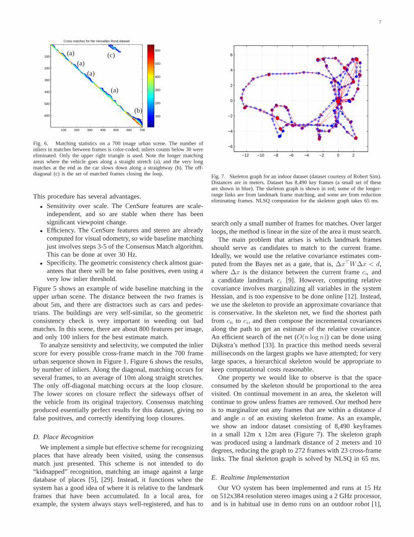
Fig. 7. Skeleton graph for an indoor dataset (dataset courtesy of Robert Sim).Distances are in meters. Dataset has 8,490 key frames (a small set of theseare shown in blue). The skeleton graph is shown in red; some ofthe longer-range links are from landmark frame matching, and some are from reductioneliminating frames. NLSQ computation for the skeleton graph takes 65 ms.

search only a small number of frames for matches. Over largerloops, the method is linear in the size of the area it must search.

The main problem that arises is which landmark framesshould serve as candidates to match to the current frame.Ideally, we would use the relative covariance estimates com-puted from the Bayes net as a gate, that is,∆x⊤W∆x < d,where∆x is the distance between the current framecn anda candidate landmarkci [9]. However, computing relativecovariance involves marginalizing all variables in the systemHessian, and is too expensive to be done online [12]. Instead,we use the skeleton to provide an approximate covariance thatis conservative. In the skeleton net, we find the shortest pathfrom cn to ci, and then compose the incremental covariancesalong the path to get an estimate of the relative covariance.An efficient search of the net (O(n log n)) can be done usingDijkstra’s method [33]. In practice this method needs severalmilliseconds on the largest graphs we have attempted; for verylarge spaces, a hierarchical skeleton would be appropriatetokeep computational costs reasonable.

One property we would like to observe is that the spaceconsumed by the skeleton should be proportional to the areavisited. On continual movement in an area, the skeleton willcontinue to grow unless frames are removed. Our method hereis to marginalize out any frames that are within a distancedand anglea of an existing skeleton frame. As an example,we show an indoor dataset consisting of 8,490 keyframesin a small 12m x 12m area (Figure 7). The skeleton graphwas produced using a landmark distance of 2 meters and 10degrees, reducing the graph to 272 frames with 23 cross-framelinks. The final skeleton graph is solved by NLSQ in 65 ms.

E. Realtime Implementation

Our VO system has been implemented and runs at 15 Hzon 512x384 resolution stereo images using a 2 GHz processor,and is in habitual use in demo runs on an outdoor robot [1],

8

0 1 2 3 4 5 6 7 8 90

1

2

3

4

5

6

Skeleton frames (1k intervals)

PC

G ti

me

(sec

onds

)

Fig. 8. Large-scale timings for a skeleton graph. The trajectory of the graphwas ∼10 km. The NLSQ time is linear in the size of the skeleton for thisgraph.

[2], [23]. At this point we have implemented the rest of theframeSLAM system only in processing logs, for which wereport timing results; we are transitioning the system to anoutdoor robot, and will report system results soon.

The main strategy for adding registration matches is to usea dual-core machine: run VO on one core, and wide-baselinematching and skeleton computations on another. Wide-baselinematching is on an “anytime” basis: we match the currentkeyframe against a set of candidates that pass the Mahalanobisgate, until the next keyframe comes in, when we start matchingthat. Whenever a good match is found, the system performsan NLSQ update, either on the whole skeleton, or a smallerarea around the current keyframe, depending on the situation.

Of course, this strategy does not address the significantproblems of frame storage and retrieval for very large systems,as done by recent place-recognition algorithms [5], [29]. Itmay also miss some matches, since it does not explore allpossible candidates. But for skeletons of less than 10k frames,where the frames can be kept in RAM, it works well.

For efficient calculation of the NLSQ updates, we use apreconditioned conjugate gradient algorithm (PCG) that hasbeen shown to have good computational properties – in manycases, the complexity increases linearly with the size of theskeleton [20]. For the large outdoor dataset, Figure 8 plotsthePCG time against the size of the skeleton. Note that these arefor a very large loop closure of a combined 10 km trajectory– typically only a small local area needs to be optimized.

V. EXPERIMENTS

It is important to test VSLAM systems on data gatheredfrom real-world platforms. It is especially important to testunder realistic conditions: narrow FOV cameras, full 3D mo-tion, and fast movement, as these present the hardest challengefor matching and motion estimation. For this research, we usedthree widely different sources of stereo frames.

1) An indoor sequence consisting of 22K frames in a smallarea, moving slowly (courtesy of Robert Sim [10]). Thestereo system had a wide FOV, narrow baseline, and waspurely planar motion.

2) An outdoor automobile sequence, the Versailles Ronddataset (courtesy of Andrew Comport [4]). This datasethas 700 frames with fast motion, 1 m baseline, narrowFOV, covering about 400 meters.

Fig. 9. Top: Indoor dataset showing raw VO (green crosses areframesand cyan dots are features) vs. frameSLAM result (red trajectory and bluefeatures). Note that the frameSLAM features correspond to arectangular setof rooms, while the VO results are skewed after the loop. Bottom: VersaillesRond urban dataset. Blue is raw VO, red is frameSLAM result (see Figure 1for cross-frame links). Note that the Z offset of the loop hasbeen corrected.

3) Two outdoor rough-terrain sequences of about 5 kmeach, from the Crusher project [6]. Baseline is 0.5 m,narrow FOV, and fast, full 3D motion with lots ofbouncing on rough terrain. These datasets offer a uniqueopportunity, for two reasons. First, they are autonomousruns through the same waypoints; they overlap and crosseach other throughout, and end up at the same place fora large loop closure. Second, the dataset is instrumentedwith both IMU and RTK GPS data, and our frameSLAMresults can be computed for both aided and unaided VO,and compared to ground truth.

A certain number of frames, about 2%, cannot bematched for VO in this dataset. We fill in these valueswith IMU data.

A. Planar Datasets

The indoor and Versailles Rond datasets were used through-out the paper to illustrate various aspects of the frameSLAMsystem. Because there is no ground truth, they offer justanecdotal evidence of performance: the indoor dataset illus-trates that the skeleton does not grow with continued traversalof a region; the Versailles Rond dataset shows loop closureover a significant distance. From the plots of Figure 9, theimprovement in fidelity to the environment is apparent. Onepossible measure of the improvement is the planarity of thetrajectories. The table below lists the relevant statistics for the

9

two runs. The timings are for NLSQ optimization of the entireskeleton.

Length Key Skeleton Planarity (m) Time(m) frames frames VO fS (ms)

Indoor 150 8.2K 272 0.15 0.11 65Versailles 370 700 133 0.19 0.15 35

B. Crusher Datasets

The Crusher data comes from two autonomous 5 km runs,which overlap significantly and form a loop. There are 20Kkeyframes in the first run, and 22K in the second. Over20 million features are found and matched in the keyframeimages, and roughly 3 times that in the total image set. Figure10 (top) gives an idea of the results from raw VO on the tworuns. There is significant deviation in all dimensions by theend of the loop (circled in red). With a skeleton of frames at5m intervals, there were a total of 1978 reduced frames, and169 wide-baseline matches between the runs using consensusmatching. These are shown as red links in the top plot.

The middle plot shows the result of applying frameSLAMto a 5m skeleton. Here the red trajectory is ground truth for theblue run, and it matches the two runs at the beginning and endof the trajectory (circled on the left). The two runs are nowconsistent with each other, but still differ from ground truthat the far right end of the trajectory. This is to be expected:the frameSLAM result will only be as good as the underlyingodometry when exploring new areas.

If VO is aided by an IMU (Section IV-B), global error isreduced dramatically. The bottom plot shows the frameSLAMresult using the aided VO – note that the blue run virtuallyoverlays the RTK GPS ground truth trajectory.

How well does the frameSLAM system reduce errors fromopen-loop VO? We should not expect any large improvementin long-distance drift at the far point of trajectories, sinceSLAM does not provide any global input that would correctsuch drift. But, we should expect dramatic gains in relativeerror, that is, between frames that are globally close, sinceSLAM enforces consistency when it finds correspondences.To show this, we compared relative pose of every frame pairto ground truth, and plotted the results as a function of distancebetween the frames. Figure 11 shows the results for both rawand aided VO. For raw VO (top plot), the open-loop errorsare very high, because of the large drift at the end of thetrajectories (Figure 10, top). With the cross-links enforcinglocal consistency, frameSLAM gives much smaller errors forshort distances, and degrades with distance, a function of yawangle drift. Note that radical reductions in the size of theskeleton, from 1/4 to 1/400 of the original keyframes, havenegligible effect, proving the accuracy of the reduced system.

A similar story exists for IMU-aided VO. Here the errorsare much smaller because of the smaller drift of VO. But thesame gains in accuracy occur for small frame distances, andagain there is almost no effect from severe skeleton reductionsuntil after 300 meters.

VI. CONCLUSIONS

We have described frameSLAM, a system for visual SLAMthat is capable of precise, realtime estimation of motion, and

0 200 400 600 800 1000 1200 14000

20

40

60

80

100

120

Distance between frames, meters

RM

S e

rror

, met

ers

VOframeSLAM

x400 reduction

x4 reduction

0 200 400 600 800 1000 1200 14002

4

6

8

10

12

14

16

Distance between frames, meters

RM

S e

rror

, met

ers

VOframeSLAM

x400reduction

x4 reduction

Fig. 11. RMS error as a function of distance. For every pair offrames, theerror in their relative pose is plotted as a function of the distance betweenthe frames. Top: Unaided VO. The blue line shows poor open-loop VOperformance, even for short distances; frameSLAM (red lines) gives excellentresults for these distances. Skeleton reduction factor hasnegligible influence.Bottom: IMU-aided VO.

also is able to keep track of local registration and globalconsistency. The key component is a skeleton system ofvisual frames, that act both as landmarks for registration,and as a network of constraints for enforcing consistency.frameSLAM has been validated through testing in a varietyof different environments, including large-scale, challengingoffroad datasets of 10 km.

We are currently porting the system to two live robotplatforms [6], [22], with the intent of providing completelyautonomous offroad navigation using just stereo vision. TheVO part of the system has already been proven over a year oftesting, but cannot eliminate the long-term drift that accruesover a run. With the implementation of the skeleton graph, weexpect to be able to assess the viability of the anytime strategyfor global registration presented in Section IV-E.

APPENDIX ANONLINEAR CONSTRAINT “ LIFTING”

Let c0, x1 and q be a set of variables with measurementcost function

∆z⊤Wi∆z (18)

and measurement vectorz. For c0 fixed at the origin, letΛ1 bethe Hessian of the reduced form of (18), according to Step 3of the Constraint Reduction algorithm. We want to show thatthe cost function

∆z′⊤

Λi∆z′ (19)

has approximately the same value at the ML estimatex1,wherez′(c0, x1) = T0x1 and z′ = x1. To do this, we showthat the likelihood distributions are approximately the same.

10

−200

−100

0

100

200

0200

400600

8001000

12001400

−50

0

50

100

150

−200

−100

0

100

200

0200

400600

8001000

12001400

020406080

−200

−100

0

100

200

0200

400600

8001000

12001400

0204060

Fig. 10. XYZ plot of two Crusher trajectories (blue and green) of about 5 km each. Top shows the raw VO, with cross-matched frames with red links. Thestart and finish of both runs is at the left, circled in red; theruns are offset vertically by 20 m at the begninning to display the links. Note the loop closurebetween the end of the blue run and the beginning of the green run. Middle shows the frameSLAM-corrected system for a 5m skeleton. The ground truth forthe blue run is in red. The relative positions of the green andblue runs have been corrected, and the loop closed. The bottom shows the excellent result forIMU-aided VO.

The cost function (18) has the joint normal distribution

P (z|x1,q) ∝ exp(−1

2∆z⊤Wi∆z) (20)

We want to find the distribution (and covariance) for thevariablex1. Let x = x1,q, andf(x) the cost function (18).Expandingf(x + δx) in a Taylor series, the cost functionbecomes

(z − f(x))⊤W (z − f(x)) (21)

≃ (z − f(x) − Jδx)⊤W (z − f(x) − Jδx) (22)

= δx⊤1 Λ1δx1 − 2∆zWJδx+ const, (23)

where we have used the Schur equality to reduce the firstterm of the third line. As∆z vanishes atx, the last formis quadratic inx1, and so is a joint normal distribution overx1. From inspection, the covariance isΛ−1

1. Hence the ML

distribution is

P (x1|z) ∝ exp(−1

2(x1 − x1)

⊤Λ1(x1 − x1)). (24)

The cost function for this PDF is (19) forc0 fixed at the origin,as required. Whenc0 is not the origin, the cost function (18)can be converted to an equivalent function by transformingall variables toc0’s coordinate system. The value stays the

same because the measurements are localized to the positionsof c0 andx1 – any global measurement, for example a GPSreading, would block the equivalence. Thus, for arbitraryc0,(20) and (24) are approximately equal just whenx1 is givenin c0’s coordinate system. Since (24) is produced by the costfunction (19), we have the approximate equivalence of the twocost functions.

REFERENCES

[1] M. Agrawal and K. Konolige. Real-time localization in outdoorenvironments using stereo vision and inexpensive gps. InICPR, August2006.

[2] M. Agrawal and K. Konolige. Rough terrain visual odometry. In Proc.International Conference on Advanced Robotics (ICAR), August 2007.

[3] M. Bosse, P. Newman, J. Leonard, M. Soika, W. Feiten, and S. Teller.An atlas framework for scalable mapping. InICRA, 2003.

[4] A. Comport, E. Malis, and P. Rives. Accurate quadrifocaltracking forrobust 3d visual odometry. InICRA, 2007.

[5] M. Cummins and P. M. Newman. Probabilistic appearance basednavigation and loop closing. InICRA, 2007.

[6] DARPA Crusher Project. http://www.rec.ri.cmu.edu/projects/autonomous/index.htm.

[7] A. Davison. Real-time simultaneaous localisation and mapping with asingle camera. InICCV, pages 1403–1410, 2003.

[8] A. J. Davison, I. D. Reid, N. D. Molton, and O. Stasse. Monoslam:Real-time single camera slam.IEEE PAMI, 29(6), 2007.

11

[9] M. Dissanayake, P. Newman, S. Clark, H. Durrant-Whyte, andM. Csorba. A solution to the simultaneous localization and map building(slam) problem.IEEE Trans. Robotics and Automation, 17(3), 2001.

[10] P. Elinas, R. Sim, and J. J. Little. sigmaslam: Stereo vision slamusing the rao-blackwellised particle filter and a novel mixture proposaldistribution. In ICRA, 2007.

[11] C. Engels, H. Stewnius, and D. Nister. Bundle adjustment rules.Photogrammetric Computer Vision, September 2006.

[12] R. M. Eustice, H. Singh, and J. J. Leonard. Exactly sparse delayed-statefilters for view-based SLAM.IEEE Trans. Robotics, 22(6), 2006.

[13] R. M. Eustice, H. Singh, J. J. Leonard, and M. R. Walter. Visuallymapping the RMS Titanic: conservative covariance estimates for SLAMinformation filters. Intl. J. Robotics Reserach, 25(12), 2006.

[14] U. Frese. A proof for the approximate sparsity of slam informationmatrices. InICRA, 2005.

[15] J. Gutmann and K. Konolige. Incremental mapping of large cyclicenvironments. InProc. IEEE International Symposium on Computa-tional Intelligence in Robotics and Automation (CIRA), pages 318–325,Monterey, California, November 1999.

[16] R. Hartley and A. Zisserman.Multiple View Geometry in ComputerVision. Cambridge University Press, 2000.

[17] T. T. Herbert Bay and L. V. Gool. Surf: Speeded up robust features. InEuropean Conference on Computer Vision, May 2006.

[18] V. S. Ila, J. Andrade, and A. Sanfeliu. Outdoor delayed-state visu-ally augmented odometry. InProc. IFAC Symposium on IntelligentAutonomous Vehicles, 2007.

[19] M. Kaess, A. Ranganathan, and F. Dellaert. iSAM: Fast incrementalsmoothing and mapping with efficient data association. InICRA, Rome,2007.

[20] K. Konolige. Large-scale map-making. InProceedings of the NationalConference on AI (AAAI), 2004.

[21] K. Konolige and M. Agrawal. Frame-frame matching for realtime con-sistent visual mapping. InProc. International Conference on Roboticsand Automation (ICRA), 2007.

[22] K. Konolige, M. Agrawal, R. C. Bolles, C. Cowan, M. Fischler, andB. Gerkey. Outdoor mapping and navigation using stereo vision. InISER, 2007.

[23] K. Konolige, M. Agrawal, and J. Sola. Large scale visual odometryfor rough terrain. InProc. International Symposium on Research inRobotics (ISRR), November 2007.

[24] D. G. Lowe. Distinctive image features from scale-invariant keypoints.International Journal of Computer Vision, 60(2):91–110, 2004.

[25] F. Lu and E. Milios. Globally consistent range scan alignment forenvironment mapping.Autonomous Robots, 4:333–349, 1997.

[26] T. K. Marks, A. Howard, M. Bajracharya, G. W. Cottrell, andL. Matthies. Gamma-slam: Stereo visual slam in unstructured envi-ronments using variance grid maps. InICRA, 2007.

[27] M. Montemerlo and S. Thrun. Large-scale robotic 3-d mapping of urbanstructures. InISER, 2004.

[28] E. Mouragnon, M. Lhuillier, M. Dhome, F. Dekeyser, and P. Sayd. Realtime localization and 3d reconstruction. InCVPR, volume 1, pages 363– 370, June 2006.

[29] D. Nister and H. Stewenius. Scalable recognition with avocabulary tree.In CVPR ’06, 2006.

[30] L. Paz, P. Jensfelt, J. Tards, and J. Neira. Ekf slam updates in o(n) withdivide and conquer slam. InICRA, 2007.

[31] G. Sibley, G. S. Sukhatme, and L. Matthies. Constant time slidingwindow filter slam as a basis for metric visual perception. InICRAWorkshop, 2007.

[32] J. Sola, M. Devy, A. Monin, and T. Lemaire. Undelayed initializationin bearing only slam. InICRA, 2005.

[33] B. Steder, G. Grisetti, C. Stachniss, S. Grzonka, A. Rottmann, andW. Burgard. Learning maps in 3d using attitude and noisy vision sensors.In IEEE International Conference on Intelligent Robots and Systems(IROS), 2007.

[34] D. Strelow and S. Singh. Motion estimation from image and inertialmeasurements. International Journal of Robotics Research, 23(12),2004.

[35] N. Sunderhauf, K. Konolige, S. Lacroix, and P. Protzel.Visual odometryusing sparse bundle adjustment on an autonomous outdoor vehicle. InTagungsband Autonome Mobile Systeme. Springer Verlag, 2005.

[36] B. Triggs, P. F. McLauchlan, R. I. Hartley, and A. W. Fitzibbon. Bundleadjustment - a modern synthesis. InVision Algorithms: Theory andPractice, LNCS, pages 298–375. Springer Verlag, 2000.

[37] R. Unnikrishnan and A. Kelly. A constrained optimization approach toglobally consistent mapping. InProceedings International Conferenceon Robotics and Systems (IROS), 2002.